A Macroeconomic View of the Shape of India’s Sovereign

ARTICLE

RBI Bulletin June 2021 49

A Macroeconomic View of the Shape of India’s Sovereign Yield Curve

* This article is prepared by Michael Debabrata Patra, Harendra Behera and Joice John, Reserve Bank of India. The authors are thankful to Sitikantha Pattanaik, Samir Ranjan Behera and K. M. Kushawaha for their comments, insightful discussions and data support. The views expressed in this article are those of the authors and do not represent the views of the Reserve Bank of India.

1 Governor’s Statement, October 9, 2020.

A Macroeconomic View of the Shape of India’s Sovereign Yield Curve*

The sovereign yield curve has a special significance for monetary policy in influencing a wide array of interest rates in the economy. Explicitly integrating macroeconomic variables with latent factors of the yield curve in a dynamic factor model, the results reveal that the level of the yield curve has undergone a downward shift from the second quarter of 2019, reflecting the ultra-accommodative stance of monetary policy. Abundant liquidity is depressing short-term interest rates more than proportionately and steepening the slope of the yield curve, alongside a pick-up in issuances of ultra-long dated paper. Global policy uncertainty impacts the slope and curvature of the yield curve, signifying the rising exposure of bond markets in India to global spillovers. Out of sample forecasts indicate scope for moderation of longer-term yields from current levels.

“Financial market stability and the orderly

evolution of the yield curve are public goods

and both market participants and the RBI have a

shared responsibility in this regard.”

Shaktikanta Das, October 20201

Towards the close of February and early March

2021, flash bond sell-offs ricocheted across major

economies and spilled over to India, steepening

sovereign yield curves everywhere. Although the

turmoil was short-lived, it dispelled the uneasy calm

that had prevailed until then. Bond markets and

monetary policy authorities faced off, both disinclined to blink first. For markets, the combination of fiscal stimulus, monetary accommodation, vaccine rollout and the release of pent-up demand translated into upward revisions in growth forecasts and in their train, inflation – the nemesis of bonds – that would force the hand of monetary authorities to abandon ultra-accommodative stances and tighten sooner than later. On the other side, central banks across the world have stressed that they remain committed to accommodation. For them, the stakes are too high to let bond traders’ expectations get ahead of outcomes and undermine the still fragile and painfully extracted economic recovery.

In India, the benchmark 10-year yield, which had averaged 5.93 per cent during April 2020 to January 2021 surged to 6.13 per cent on February 2 on the announcement of the market borrowing programme of the central government. Following the announcement of a slew of measures by the Reserve Bank of India (RBI) on February 5, the benchmark yield eased to 5.96 per cent by February 11. Thereafter, global spillovers referred to earlier sparked a stampede; by March 5, the benchmark yield in India had touched 6.23 per cent, but the RBI’s announcements of large-sized operation twists soothed frayed nerves and settled it at around 6.21 per cent on March 9. It has eased considerably since then and was trading range bound around 6 per cent at the time of this article going to print.

The sovereign yield curve has a special significance for monetary policy. In fact, in extraordinary times characterised by unconventional monetary policy actions and stances, it is the centrepiece in policy setting. First, with policy rates at the zero bound, the usual channel of monetary policy transmission is dormant. Accordingly, policy makers have sought to leapfrog into the longer end of the interest rate structure in order to influence financial conditions more directly. Second, the sovereign yield curve is

the benchmark off which other financial instruments

are priced (Das, 2020a). By impacting the yield

ARTICLE

RBI Bulletin June 202150


curve, central banks can influence a wider array of interest rates in the economy and thereby, overall cost conditions. Third, the yield curve offers valuable insights into the behaviour of risk premia, which provides clues as to how monetary policy should respond to these exogenous factors. Fourth, the yield curve embeds expectations about future growth and inflation once risk premia are separated out, and this is a useful guide for the conduct of forward-looking monetary policy. Fifth, for central banks that are also issuers of public debt by mandate, a good understanding of yield curve dynamics helps to place the debt in the market at minimum cost and rollover risk. Finally, policy makers can draw information from the term structure of yields to learn about the market’s expectations of monetary policy.

The yield is a combination of the short-term interest rate typically set by the central bank, the expected future short-term interest rate typically embodied in the monetary policy stance, and the term premium. As the term premium is not directly observable, it has to be modelled under some assumptions. Early models were based on the expectations hypothesis of the term structure of interest rates, which posited the yield to be the average expected level of short-term interest rates over the maturity period of the bond (Fisher, 1896; Froot, 1989). There is, however, weak empirical support for the expectations hypothesis (Gürkaynak and Wright, 2012). Another approach is the market segmentation hypothesis which states that long and short-term interest rates are not related to each other and should be viewed separately like items in different markets (Campbell, 1980). Yield curves are determined by supply and demand forces within each market/category of debt security, and the yields for one category of maturities cannot be used to predict the yields for a different category of maturities. The market for each segment derives from specific investor preferences in terms of durations, bond characteristics, and investment habits (Ang and Piazzesi, 2003). The segmented markets hypothesis

can at best be used to explain any particular shape of the yield curve, although it fits positive sloping curves the best. It cannot be used, however, to interpret the whole yield curve in whatever shape it may be, and therefore offers no information content during analysis, i.e., by itself, it is not sufficient (Taylor and Masson, 1991; Gürkaynak and Wright, 2012). In the finance literature, factor models are popular and usually impose a no-arbitrage restriction – securities with the same risk characteristics have the same price. In these models, unobserved or latent factors explain the yield structure and they are typically classified as the level, the slope and the curvature. They are, however, bereft of any information on macroeconomic conditions under which yields are known to form. At the other end of the spectrum are models that rely on macroeconomic determinants of the yield curve (Diebold et al., 2006).

This article joins a recent and rapidly growing strand in the literature in explicitly integrating macroeconomic determinants into a baseline latent factor model. Seminal work in this field preferred a model in which macroeconomic and financial variables are integrated in order to estimate the yield curve by considering two-way causality – components of yield curve to macroeconomic variables, and vice versa – so that potential bi-directional feedback from the yield curve to the economy and back are nested in the model (Diebold et al., 2006). In this article, we build on this work by incorporating additional macro variables to capture open economy dynamics as well as the RBI’s liquidity and market borrowing strategies. Bayesian methods are applied to estimate the model parameters as they are efficient in dealing with unobserved variables. The results indicate that our hybrid model predicts the observed yields well. They also reveal that the level of the yield curve has undergone a downward shift from the second quarter of 2019, reflecting the impact of ultra-accommodative monetary policy on longer-term yields; however, there has been a steepening of the yield curve due

ARTICLE



to abundant liquidity depressing short-term interest

rates and a pick-up in issuances of ultra-long dated

papers. Among other macroeconomic determinants,

global policy uncertainty impacts the slope and

curvature of the yield curve, signifying the rising

exposure of bond markets in India to global spillovers.

The rest of the article is organised into four

sections. Section II presents some stylised facts on

recent yield curve dynamics, and the factors that

influence the government securities (g-sec) market

in India. Section III discusses a methodological

framework to find out the determinants of the yield

curve, and the results therefrom are presented in

Section IV. Section V concludes the article with some

policy perspectives.

II. Recent Bond Market Developments

Across the world, central banks responded to the

outbreak of the COVID-19 pandemic by engendering

easy financial conditions through the provision of

abundant liquidity via bond purchases and balance

sheet policies. As a result, bond yields eased to all-

time lows through 2020 and set the stage for record

corporate issuances as well as strong rallies in equities.

In India, where a similar sequence characterised

the interface between markets and the monetary

authority, the overriding objective was to prevent

financial markets from freezing up and to ensure

normal functioning of financial intermediaries;

ease the stress faced by households and businesses

so as to keep the life blood of finance flowing (Das,

2020b). Accordingly, the RBI carefully steered yields,

emphasising an orderly evolution of the yield curve

(Das, 2021a). This guidance was reinforced in both

primary and secondary market operations by auction

cut-offs, devolvements, cancellations and exercise of

green shoe options (Chart 1).

Borrowing costs in financial markets dropped to

their lowest in a decade on the back of policy rate

reductions and abundant liquidity. Interest rates

on short-term treasury bills, commercial paper (CP)

and certificates of deposit (CD) fully priced in the

reduction in the policy rate and, in fact, traded below

it (Chart 2a). The weighted average cost of borrowings

Chart 1: Monetary Policy and Sovereign Yields

a. Policy Rate and Sovereign Yields b. Benchmark 10-year G-sec Yield

Sources: Reserve Bank of India; Thomson Reuters’ Eikon.

ARTICLE



in the gilt market dropped to its lowest level in 16

years (Das, 2020c). Spreads between corporate and

g-sec rates were compressed across all maturities and

rating categories of corporate bonds (Chart 2b).

II.1 The Global Context

As vaccination drives gathered speed and scale

in some advanced economies towards the close of

2020, financial markets across the world caught the

winds of reflation trade as hopes of a quicker global

recovery revived. Equity and credit markets extended

gains in spite of stretched valuations, and the return

of risk-on sentiments spurred a search for yield as

capital flows surged into emerging markets in January

2021 on the back of a weaker US dollar. Market-based

inflation expectations hardened and bond markets

began to believe that central banks would be forced

to normalise, with inflation looking likely to exceed

targets substantially as the recovery gained traction.

Globally, high uncertainty clouded the outlook for

monetary policy and chatter on taper tantrums

and failed normalisations of the past rent the air.

Subsequently, U.S. treasury yields started rising and

surged to their highest level in a year on March 31,

2021. This development spilled over and led to a rise

in term premia across the advanced and emerging

market economies (Chart 3)2. Among EMEs, the term

premium rose to as high as 500 basis points (bps) in

South Africa, around 400 bps in Latin America and

in the range of 65-300 bps in Asia (225 bps in India).

In countries like Japan and Australia where yield

control is the dominant objective of monetary policy,

term premia have remained low and stable or have

declined.

II.2 Bond Market Dynamics in India

In India, the announcement of the government’s

borrowing programme in February was the trigger,

but in hindsight, it is evident that the surge in

the term premium in the beginning of 2021 was

in tandem with the increasing global economic

Chart 2: Co-movement of Sovereign Yields and Interest Rates in Other Segments

a. Money Market Interest Rates: 3 Month Maturity b. Bond Market: Yields at 5-year Maturity

Sources: Reserve Bank of India; Thomson Reuters’ Eikon; Bloomberg.

2 Term premium is calculated by taking the difference between the yields on 10-year and 1-year g-secs.

ARTICLE



policy uncertainty (Chart 4), pointing to the rising

sensitivity of the term premium to global spillovers

(Patra et al., 2020).

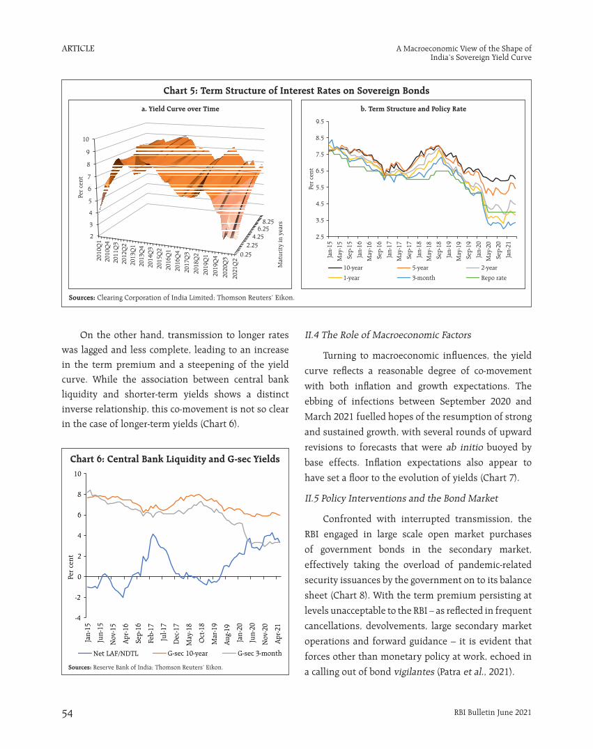
II.3 A Cross-sectional View

Investigating the steepening of India’s yield

curve cross-sectionally and over time (Chart 5a), it

is observed that yields across the maturity spectrum

have declined, but more at the short end than at the

longer end (Chart 5b). Thus, monetary policy has been

effective in pulling down and anchoring short-term

interest rates which, in turn, facilitated the easing of

rates right up to two years maturity even below the

policy rate.

Chart 3: Movements of Term-premia

a. Advanced Economies b. Emerging Market Economies

Source: Thomson Reuters’ Eikon.

Chart 4: Global Economic Policy Uncertainty and Term Premia

Sources: Thomson Reuters’ Eikon; https://www.policyuncertainty.com.

ARTICLE



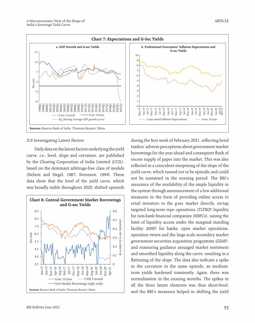
On the other hand, transmission to longer rates

was lagged and less complete, leading to an increase

in the term premium and a steepening of the yield

curve. While the association between central bank

liquidity and shorter-term yields shows a distinct

inverse relationship, this co-movement is not so clear

in the case of longer-term yields (Chart 6).

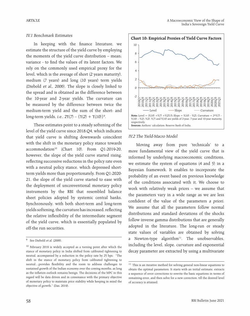
II.4 The Role of Macroeconomic Factors

Turning to macroeconomic influences, the yield

curve reflects a reasonable degree of co-movement

with both inflation and growth expectations. The

ebbing of infections between September 2020 and

March 2021 fuelled hopes of the resumption of strong

and sustained growth, with several rounds of upward

revisions to forecasts that were ab initio buoyed by

base effects. Inflation expectations also appear to

have set a floor to the evolution of yields (Chart 7).

II.5 Policy Interventions and the Bond Market

Confronted with interrupted transmission, the

RBI engaged in large scale open market purchases

of government bonds in the secondary market,

effectively taking the overload of pandemic-related

security issuances by the government on to its balance

sheet (Chart 8). With the term premium persisting at

levels unacceptable to the RBI – as reflected in frequent

cancellations, devolvements, large secondary market

operations and forward guidance – it is evident that

forces other than monetary policy at work, echoed in

a calling out of bond vigilantes (Patra et al., 2021).

Chart 5: Term Structure of Interest Rates on Sovereign Bonds

a. Yield Curve over Time b. Term Structure and Policy Rate

Sources: Clearing Corporation of India Limited; Thomson Reuters’ Eikon.

Chart 6: Central Bank Liquidity and G-sec Yields


-4

-2

0

2

4

6

8

10

Jan-

15

Jun-

15

Nov

-15

Apr

-16

Sep-

16

Feb-

17

Jul-1

7

Dec

-17

M-

ay18

Oct

-18

Mar

-19

Aug-

19

Jan-

20

Jun-

20

Nov

-20

Apr

- 12

Per

cent

Net AL F/NDTL G-sec 10-year G-sec 3-month

ARTICLE



II.6 Investigating Latent Factors

Daily data on the latent factors underlying the yield

curve, i.e., level, slope and curvature, are published

by the Clearing Corporation of India Limited (CCIL),

based on the dominant arbitrage-free class of models

(Nelson and Siegel, 1987; Svensson, 1994). These

data show that the level of the yield curve, which

was broadly stable throughout 2020, shifted upwards

during the first week of February 2021, reflecting bond traders’ adverse perceptions about government market borrowings for the year ahead and consequent flush of excess supply of paper into the market. This was also reflected in a coincident steepening of the slope of the yield curve, which turned out to be episodic and could not be sustained in the ensuing period. The RBI’s assurance of the availability of the ample liquidity in the system through announcement of a few additional measures in the form of providing online access to retail investors to the g-sec market directly, on-tap targeted long-term repo operations (TLTRO) liquidity for non-bank financial companies (NBFCs), raising the limit of liquidity access under the marginal standing facility (MSF) for banks, open market operations, operation twists and the large-scale secondary market government securities acquisition programme (GSAP), and reassuring guidance assuaged market sentiment and smoothed liquidity along the curve, resulting in a flattening of the slope. The data also indicate a spike in the curvature in the same episode, as medium-term yields hardened transiently. Again, there was normalisation in the ensuing months. The spikes in all the three latent elements was thus short-lived,

and the RBI’s measures helped in shifting the yield

Chart 7: Expectations and G-Sec Yields

a. GDP Growth and G-sec Yields b. Professional Forecasters’ Inflation Expectations and G-sec Yields


Chart 8: Central Government Market Borrowings and G-sec Yields


ARTICLE



curve downward as observed in a decline in level, slope and curvature by 483 bps, 472 bps and 232 bps, respectively, during February 4 and 5 (Chart 9).

III. Model Structure

Our estimation framework essentially follows the tradition of the dynamic latent factor approach augmented with macroeconomic variables representing real activity, inflation, and the monetary policy stance (Diebold et al., 2006). In addition, we include global factors, liquidity conditions and government market borrowing programme in the augmented model. We introduce a time-varying structure by allowing the latent variables - level3, slope4, and curvature5 - to follow an autoregressive process, which is preferred in the literature over the random walk process as the latter is a non-stationary

progression.

The yields at any maturity ( ) is decomposed as

follows:

...(1)

Where Lt, St and Ct are the level, slope and

curvature, respectively, and are unobserved and time-

varying. The parameter , the exponential decay rate6,

is also time-varying.

The estimation of the structure of the yield curve

and its dynamic interaction with macroeconomic and

global variables is carried out by formulating a state-

space representation which describes how observable

variables relate to the latent variables and how they

evolve over time. The measurement equation is

formulated by relating the observed yields to the

unobserved factors, i.e., level, slope and curvature, in

a matrix representation:

... (2)

Where ... (3)

Chart 9: India’s Sovereign Bond Yield Curve

a. Slope and Curvature b. Shifts in Yield Curve

Source: Clearing Corporation of India Limited.

3 Level is the average of yields across maturities.

4 Slope is the long-term rate minus the short-term rate..

5 Curvature is the relationship between yields at short, medium and longer maturities – the difference between twice the medium-term rate and the sum of the short-term rate and the long-term rate. Higher curvature indicates that the medium-term rate is higher than the short-term rate and the long-term rate, which shows up as a hump in the yield curve.

6 Exponential decay describes the process of reduction of slope and curvature by a consistent percentage rate over a period of time.

ARTICLE



This is the yield-only model, which we use

as a benchmark to evaluate the gains in accuracy

when augmenting it with macroeconomic variables

described earlier in a yield-macro model (Diebold et

al,, 2006). Our model allows the dynamic two-way

interaction of macro variables with the structure of

the yield curve with feedback.

Thus, our dynamic latent factor yield-macro

model for estimating the yield curve in India is based

on the following set of measurement and transition

equations:

Where is guided by equation (1) ... (4)

Where

and

,

where

... (5)

Real activity is represented by the output gap

(OG), the inflation gap with inflation (INF) measured

as seasonally adjusted quarter on quarter changes in

the consumer price index (CPI) and monetary policy

which is proxied by the weighted average call money

rate (WACR) – its operating target. Liquidity conditions

or LIQU, are captured by the outstanding absorption/

injection under the RBI’s liquidity adjustment facility

(LAF) as a proportion to banks’ net demand and

time liabilities. The government market borrowing

programme is proxied by the market borrowing to

market turnover ratio (GMB) and global uncertainty

is represented by the Global Economic Policy

Uncertainty index (GEPU) 7. LIQU, GMB and GEPU are

treated as exogenous variables and are assumed to

evolve independently of the yield curve factors and

other macro developments – they are allowed to affect

only the yield curve factors and not the other macro

variables directly.

The model is estimated by using Bayesian methods

which score over other time series approaches in

dealing with a large number of parameters over

relatively short time periods. The unobservables

(latent variables) are filtered out by using a multivariate

Kalman filter8.

IV. Results

The model is estimated for the period spanning

the first quarter of 2010 to the corresponding quarter

of 2021 on quarterly data on Indian government

security yields of maturities of 2 to 10 years. All data

are sourced from the Database on Indian Economy

(DBIE) of the RBI, except GEPU, which is obtained as

discussed in footnote 7.

7 The GEPU Index is a GDP-weighted average of national EPU indices for 21 countries, each reflecting the relative frequency of own-country newspaper articles that contain a trio of terms pertaining to the economy (E), policy (P) and uncertainty (U). The data are available at https://www.policyuncertainty.com/global_monthly.html

8 The Kalman filter is an algorithm to estimate unknown/unobservable variables from a set of observed variables over time. When more than one observable variable is involved, the process is called multivariate. These estimates tend to be more accurate than those based on a single observable variable alone. Additionally, the Kalman filter produces estimates with greater precision as compared to other estimation methods.

ARTICLE



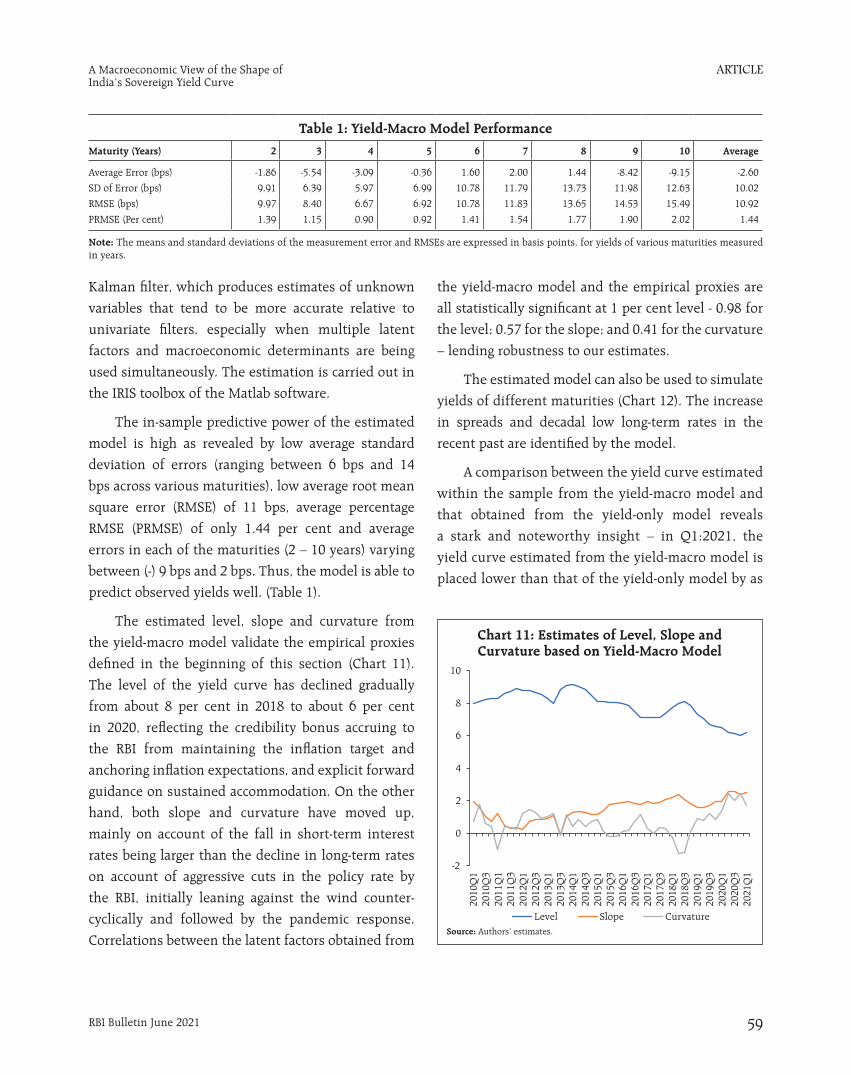
IV.1 Benchmark Estimates

In keeping with the finance literature, we estimate the structure of the yield curve by employing the moments of the yield curve distribution – mean; variance - to find the values of its latent factors. We rely on the commonly used empirical proxy for the level, which is the average of short (2 years maturity), medium (7 years) and long (10 years) term yields (Diebold et al,, 2006). The slope is closely linked to the spread and is obtained as the difference between the 10-year and 2-year yields. The curvature can be measured by the difference between twice the medium-term yield and the sum of the short- and long-term yields, i.e., 2Y(7) – {Y(2) + Y(10)}9.

These estimates point to a steady softening of the level of the yield curve since 2018:Q4, which indicates that yield curve is shifting downwards coincident with the shift in the monetary policy stance towards accommodation10 (Chart 10). From Q1:2019-20, however, the slope of the yield curve started rising, reflecting successive reductions in the policy rate even with a neutral policy stance, which depressed short-term yields more than proportionately. From Q1:2020-21, the slope of the yield curve started to ease with the deployment of unconventional monetary policy instruments by the RBI that resembled balance sheet policies adopted by systemic central banks. Synchronously, with both short-term and long-term yields softening, the curvature has increased, reflecting the relative inflexibility of the intermediate segment of the yield curve, which is essentially populated by

off-the run securities.

IV.2 The Yield-Macro Model

Moving away from pure ‘technicals’ to a

more fundamental view of the yield curve that is

informed by underlying macroeconomic conditions,

we estimate the system of equations (4 and 5) in a

Bayesian framework. It enables to incorporate the

probability of an event based on previous knowledge

of the conditions associated with it. We choose to

work with relatively weak priors – we assume that

the parameters vary in a wide range as we are less

confident of the value of the parameters a priori. We assume that all the parameters follow normal

distributions and standard deviations of the shocks

follow inverse gamma distributions that are generally

adopted in the literature. The long-run or steady

state values of variables are obtained by solving

a Newton-type algorithm11. The unobservables,

including the level, slope, curvature and exponential

decay parameter are extracted by using a multivariate

9 See Diebold et al. (2006).

10 February 2019 is widely accepted as a turning point after which the stance of monetary policy in India shifted from calibrated tightening to neutral, accompanied by a reduction in the policy rate by 25 bps: “The shift in the stance of monetary policy from calibrated tightening to neutral…provides flexibility and the room to address challenges to sustained growth of the Indian economy over the coming months, as long as the inflation outlook remains benign. The decisions of the MPC in this regard will be data driven and in consonance with the primary objective of monetary policy to maintain price stability while keeping in mind the objective of growth.” (Das, 2019).

Chart 10: Empirical Proxies of Yield Curve Factors

Note: Level = (Y(10) +Y(7) +Y(2))/3; Slope = Y(10) – Y(2); Curvature = 2*Y(7) – Y(10) – Y(2); Y(2), Y(7) and Y(10) are yields of 2-year, 7-year and 10-year maturity, respectively. Sources: Authors’ calculation; Reserve Bank of India.

11 This is an iterative method for solving general non-linear equations to obtain the optimal parameters. It starts with an initial estimate, extracts a sequence of error corrections to rewrite the basic equations in terms of remaining error, and then solve for a new correction, till the desired level of accuracy is attained.

ARTICLE



Chart 11: Estimates of Level, Slope and Curvature based on Yield-Macro Model

Source: Authors’ estimates.

Kalman filter, which produces estimates of unknown

variables that tend to be more accurate relative to

univariate filters, especially when multiple latent

factors and macroeconomic determinants are being

used simultaneously. The estimation is carried out in

the IRIS toolbox of the Matlab software.

The in-sample predictive power of the estimated

model is high as revealed by low average standard

deviation of errors (ranging between 6 bps and 14

bps across various maturities), low average root mean

square error (RMSE) of 11 bps, average percentage

RMSE (PRMSE) of only 1.44 per cent and average

errors in each of the maturities (2 – 10 years) varying

between (-) 9 bps and 2 bps. Thus, the model is able to

predict observed yields well. (Table 1).

The estimated level, slope and curvature from

the yield-macro model validate the empirical proxies

defined in the beginning of this section (Chart 11).

The level of the yield curve has declined gradually

from about 8 per cent in 2018 to about 6 per cent

in 2020, reflecting the credibility bonus accruing to

the RBI from maintaining the inflation target and

anchoring inflation expectations, and explicit forward

guidance on sustained accommodation. On the other

hand, both slope and curvature have moved up,

mainly on account of the fall in short-term interest

rates being larger than the decline in long-term rates

on account of aggressive cuts in the policy rate by

the RBI, initially leaning against the wind counter-

cyclically and followed by the pandemic response.

Correlations between the latent factors obtained from

the yield-macro model and the empirical proxies are

all statistically significant at 1 per cent level - 0.98 for

the level; 0.57 for the slope; and 0.41 for the curvature

– lending robustness to our estimates.

The estimated model can also be used to simulate

yields of different maturities (Chart 12). The increase

in spreads and decadal low long-term rates in the

recent past are identified by the model.

A comparison between the yield curve estimated

within the sample from the yield-macro model and

that obtained from the yield-only model reveals

a stark and noteworthy insight – in Q1:2021, the

yield curve estimated from the yield-macro model is

placed lower than that of the yield-only model by as

Table 1: Yield-Macro Model PerformanceMaturity (Years) 2 3 4 5 6 7 8 9 10 Average

Average Error (bps) -1.86 -5.54 -3.09 -0.36 1.60 2.00 1.44 -8.42 -9.15 -2.60

SD of Error (bps) 9.91 6.39 5.97 6.99 10.78 11.79 13.73 11.98 12.63 10.02

RMSE (bps) 9.97 8.40 6.67 6.92 10.78 11.83 13.65 14.53 15.49 10.92

PRMSE (Per cent) 1.39 1.15 0.90 0.92 1.41 1.54 1.77 1.90 2.02 1.44

Note: The means and standard deviations of the measurement error and RMSEs are expressed in basis points, for yields of various maturities measured in years.

ARTICLE



much as 17 bps for the 10-year maturity (Chart 13).

The out of sample forecasts of the yield curve for the

second quarter of 2021 suggest a further moderation

in yields in the medium to long maturity, with the

benchmark 10-year yield is estimated at 5.87 per

cent (Table 2). This underscores the importance of

considering macroeconomic determinants in an

unbiased assessment of the shape of the yield curve

in India.

As Table 2 shows, estimates of the yield curve

drawn from the yield-only model tend to fit the

data well within-the-sample, but do not provide any

insights into the underlying behavior of the latent

factors. Furthermore, precision tend to decay out of

sample as these estimates are bereft of macroeconomic

underpinnings. In the face of the exceptional

circumstances like the pandemic, idiosyncratic market

behaviour tends to disproportionately influence out-

of-sample estimation results from the yield-only

model.

Impulse responses of the latent factors to a unit

shock to the macroeconomic variables depicts their

interactions, enabling an empirical evaluation of the

priors available in the literature (Chart 14).

Chart 13: Estimated Yield Curve for Q1:2021


Table 2: Model based Yield Forecasts(Per cent)

Maturity (in Years)

ActualQ1:2021

In Sample Forecasts for Q1:2021 Out of Sample Forecasts for Q2:2021 Q3:2021

Yield Only Model Yield-Macro Model Yield Only Model Yield-Macro Model# Yield-Macro Model

2 4.41 4.12 4.13 4.95 4.46 4.863 4.91 4.93 4.87 5.47 4.99 5.264 5.31 5.39 5.30 5.76 5.29 5.495 5.73 5.68 5.56 5.95 5.48 5.646 6.01 5.88 5.74 6.07 5.61 5.737 6.21 6.02 5.87 6.16 5.70 5.808 6.31 6.13 5.97 6.23 5.77 5.869 6.22 6.21 6.04 6.28 5.82 5.9010 6.26 6.27 6.10 6.32 5.87 5.93

#: For Q2 and Q3: 2021, out-of-sample forecasts are generated by using the RBI’s forecasts for GDP growth and inflation and assuming the average levels of LAF, GMB and GEPU observed up to May to prevail.

Chart 12: Predicted Yields from the Yield- Macro Model


6.10

5.30

4.13

6.27

6.10

ARTICLE



Chart 14: Impulse Response of Macro Shocks on Yield Curve Factors

Responses

Shocks

Level Slope Curvature

a. WACR [Shock: 1 ppt Decline]

b. Liquidity (Per cent NDTL) [Shock: 1 ppt Increase]

c. Inflation [Shock: 1 ppt Increase]

d. Output Gap [Shock: 1ppt Decline]

e. GEPU [Shock: 10 ppt Increase]

f. GMB (Per cent Turnover) [Shock: 0.1 ppt Increase]


ARTICLE



A decline in the policy rate has an immediate

positive impact on the slope of the yield curve as

the impact of the policy rate change is swiftly and

completely transmitted to short-term maturities,

causing the yield curve to become steeper

(Chart 14a). This is in line with the cross-country

experience (Vargas, 2005; Diebold et al., 2006; Fan and

Johansson, 2010).

When liquidity increases by one percentage point

(ppt)12, the level of the yield curve declines by 5 bps,

accompanied by a reduction in the slope by 16 bps.

The increase in liquidity has a cooling effect across

the yield spectrum, but with a relatively larger impact

on the long-term rates: by reducing the risk premium,

the injection of liquidity flattens the yield curve. The

impact of liquidity on the curvature is unambiguous,

producing a steepening of the yield curve in the

medium to long-term segment as off-the-run securities

turn increasingly illiquid (Chart 14b).

A one percentage point change in inflation relative

to the target changes the level of the yield curve by

13 bps as expectations of market participants about

future interest rates adapt in response. The slope

also adjusted by 28 bps, indicating that long-term

rates respond relatively more aggressively to inflation

developments (Chart 14c).

If the output gap reduces by one percentage point

and turns negative under the impact of a shock, it

reduces the level and curvature and increases the

slope, mimicking the response of the yield curve to a

reduction in the policy rate (Chart 14d).

An increase in GEPU by 10 percentage points raises

the slope by 12 bps - global policy uncertainty raises

risk premia. The rise in the slope can be interpreted as

either agents’ expectation of an accommodative policy

response (as in the case of the COVID-19 pandemic) or hardening of long-term interest rates in response to excessive uncertainty. The curvature also increases in response to heightened uncertainty and is reflected in a steepening of the yield curve at the short- to medium maturity segment (Chart 14e).

An increase in government market borrowing (0.1 ppt increase in turnover ratio) has a positive impact on the level, raising it by 7 bps, but it has a minimal impact on the slope and the curvature – because the expansion in the borrowing programme increases yields across the spectrum (Chart 14f).

V. Conclusion

In these extraordinary times, recent developments in gilt markets in India as well as in the rest of the world present a term premium conundrum. Market participants sneeze when large government borrowing programmes are announced and/or when their inflation expectations are aroused. Central banks struggle to prevent them from catching a cold by taking down policy rates to as low as they can, even to the zero bound and below. They also undertake open market operations that inject liquidity and take out bonds from market turnover. They relieve supply pressures in the market at the cost of bloating their own balance sheets, warranting additional provision for market risk. Central banks also provide calming communication that assure ‘low’ and ‘ample’ for longer as they look through inflation fears on their path of reviving economic growth.

Without a doubt, it takes at least two views to make a market and derive efficient outcomes. In the recent period, however, when market processes of price discovery and efficient resource allocation have been overwhelmed by the pandemic, the search for cooperative solutions is often sacrificed at the altar of face offs. Market participants seek to outguess and front run central banks who, on their part, believe that markets are idiosyncratic and have to be intervened to produce competitive outcomes. To summarise the lessons gleaned,

12 One percentage point increase in liquidity represents an increase in injection of liquidity through the LAF as a ratio of banks’ NDTL (which is the metric for banks’ access to liquidity from the RBI). This is equivalent to Rs. 1.5 lakh crore on current basis.

ARTICLE



• When the traditional channels of transmissionof monetary policy are frozen because of risk aversion and absent demand, central banks have to turn to market-based channels of transmission to ensure congenial financial conditions for the recovery. In such situations, the gilt yield, off which other financial instruments are priced, becomes a variable that it is more important for monetary policy than debt management, and

hence, macroeconomic conditions should be

taken into account in any assessment of the level,

slope and curvature of the yield curve.

• Monetary policy is a potent instrument for

influencing the term structure of interest rates -

policy rate changes tend to impact the slope of

the yield curve, while liquidity impacts the level

as well as the slope of the yield curve, rendering it

a better instrument for managing the yield curve.

• Managing inflation expectations, including

through effective communication, should be part

of any strategy to manage the yield curve, since

changes in inflation expectations impact the

level, slope and curvature of the yield curve and

can counteract the monetary policy stance.

• The empirical results obtained in this paper

indicate that a yield-only model tends to

overpredict the level of yields across the

spectrum except 6-8 years maturities segment

(Table 2; Annex). Comparing actual yields for

Q2:2021 (up to June 10) with the forecasts, the

yield-macro model point to the scope for yields

to adjust upwards by 1-23 bps in the 2-3 years

maturity segment and downwards by 39-56 bps

in the 6-9 years segment. It finds the 5-year

yield to be fairly valued and the 10-year yield

converging to fair value in Q2:2021. In Q3 (July-

September 2021), the estimates show that there

is further scope for the 10-year yield to ease

from current levels. These evolving yield curve

dynamics suggest the scope for open market

operations and the points on the yield curve to

which they need to be targeted.

ARTICLE



Annex

Chart 1A: Yields - Actual vs. Out of Sample Forecasts

Source: Authors’ estimates; Thomson Reuters’ Eikon.

6.03

5.87

6.32

5.93

4.0

4.5

5.0

5.5

6.0

6.5

2 3 4 5 6 7 8 9 10

Per

cent

Actual 2021: Q2 (up to June 10) Yie - 2 21 2ld Macro Model 0 :Q Yield Only Model 2021:Q2 Yie - 2 21 3ld Macro Model 0 :Q

ARTICLE



References

Ang, A., and Piazzesi, M. (2003). A No-arbitrage Vector

Autoregression of Term Structure Dynamics with

Macroeconomic and Latent Variables. Journal of

Monetary Economics, 50(4), 745-787.

Campbell, T. S. (1980). On the Extent of Segmentation

in the Municipal Securities Market. Journal of Money,

Credit and Banking, 12(1), 71-83.

Das, S. (2019). Statement by Governor - Sixth Bi-

monthly Monetary Policy Press Conference for 2018-

19, February, Reserve Bank of India.

Das, S. (2020a). Governor’s Statement, December 4,

2020, Reserve Bank of India.

Das, S. (2020b). Governor’s Statement, August 6, 2020,

Reserve Bank of India.

Das, S. (2020c). Governor’s Statement, October 9,


Das, S. (2021a). Governor’s Statement, February 5,


Das, S. (2021b). Edited Transcript of Reserve Bank of

India’s Monetary Policy Press Conference, June 04,

Reserve Bank of India.

Diebold, F. X., and Li, C. (2006). Forecasting the Term

Structure of Government Bond Yields. Journal of

Econometrics, 130(2), 337-364.

Diebold, F. X., Rudebusch, G. D., and Aruoba, S. B.

(2006). The Macroeconomy and the Yield Curve:

A Dynamic Latent Factor Approach. Journal of

Econometrics, 131(1-2), 309-338.

Fan, L., and Johansson, A. C. (2010). China’s Official

Rates and Bond Yields. Journal of Banking and Finance,

34(5), 996-1007.

Fisher, I. (1896). Appreciation and Interest. Publications

of the American Economic Association, 11, 21-29.

Froot, K. A. (1989). New Hope for the Expectations

Hypothesis of the Term Structure of Interest Rates. The

Journal of Finance, 44(2), 283-305.

Gürkaynak, R. S., and Wright, J. H. (2012).

Macroeconomics and the Term Structure. Journal of

Economic Literature, 50(2), 331-67.

Nelson, C. R., and Siegel, A. F. (1987). Parsimonious

Modeling of Yield Curves. Journal of Business, 60(4),

473-89.

Patra, M.D., Behera, H. and John, J. (2020). Revisiting

the Determinants of the Term Premium in India.

RBI Bulletin, Reserve Bank of India, November.

Patra, M.D., et al. (2021). State of the Economy.

RBI Bulletin, Reserve Bank of India, May.

Taylor, M.P. and Masson, P.R. (1991). Modelling the

Yield Curve. IMF Working Paper, December.

Svensson, L. E. (1994). Estimating and Interpreting

Forward Interest Rates: Sweden 1992-1994. NBER

Working Paper, No. w4871, National Bureau of

Economic Research.

Vargas, G. A. (2005). Macroeconomic Determinants

of the Movement of the Yield Curve. MPRA Working

Papers, March.

Documents

A Macroeconomic View of the Shape of India’s Sovereign