Embed Size (px)
Citation preview
A Master Theorem for Discrete Divide and Conquer Recurrences∗
Michael Drmota† Wojciech Szpankowski‡
Dedicated to Philippe Flajolet 1948-2011
Abstract
Divide-and-conquer recurrences are one of the most studied equations in computer science.Yet, discrete versions of these recurrences, namely
T (n) = an +
m∑
j=1
bjT (⌊pjn + δj⌋) +
m∑
j=1
bjT(⌈
pjn + δj
⌉)
for some known sequence an and given bj , bj , pj and δj , δj , present some challenges. The discretenature of this recurrence (represented by the floor and ceiling functions) introduces certainoscillations not captured by the traditional Master Theorem, for example due to Akra and Bazziwho primary studied the continuous version of the recurrence. We apply powerful techniquessuch as Dirichlet series, Mellin-Perron formula, and (extended) Tauberian theorems of Wiener-Ikehara to provide a complete and precise solution to this basic computer science recurrence. Weillustrate applicability of our results on several examples including a popular and fast arithmeticcoding algorithm due to Boncelet for which we estimate its average redundancy and prove theCentral Limit Theorem for the phrase length. To the best of our knowledge, discrete divide andconquer recurrences were not studied in this generality and such detail; in particular, this allowsus to compare the redundancy of Boncelet’s algorithm to the (asymptotically) optimal Tunstallscheme.
Key Words: Divide-and-conquer recurrence, mergesort, Karatsuba algorithm, Strassen algorithm,Boncelet’s data compression algorithm, Dirichlet series, Mellin-Perron formula, Tauberian theorem.
∗The work of these authors was supported in part by the Austrian Science Foundation FWF Grant No. S9604,
by NSF Science and Technology Center Grant CCF-0939370, NSF Grants DMS-0800568 and CCF-0830140, AFOSR
Grant FA8655-11-1-3076, and NSA Grant H98230-11-1-0141.†Inst. Discrete Mathematics and Geometry, TU Wien, A-1040 Wien, Austria, [email protected].‡Department of Computer Science, Purdue University, West Lafayette, IN 47907-2066 U.S.A., [email protected]
1

1 Introduction
Divide and conquer is a very popular strategy to design algorithms. It splits the input into severalsmaller subproblems, solving each subproblem separately, and then knitting together to solve theoriginal problem. Typical examples include heapsort, mergesort, discrete Fourier transform, queues,sorting networks, compression algorithms, and so forth [15, 7, 23, 27, 31]. While it is relatively easyto determine the general growth order for the algorithm complexity, a precise asymptotic analysisis often appreciably more subtle. Our goal is to present such an analysis for discrete divide andconquer recurrences.
The complexity of a divide and conquer algorithm is well described by its divide and conquerrecurrence. We assume that the problem is split into m subproblems. It is natural to assume thatthere is a cost associated with combining subproblems together to find the solution. We denotesuch a cost by an, where n is the size of the original problem. In addition, each subproblem maycontribute in a different way to the final solution; we represent this by coefficients bj and bj for1 ≤ j ≤ m. Finally, we postulate that the original input n is divided into subproblems of size ⌊hj(n)⌋and ⌈hj(n)⌉, 1 ≤ j ≤ m, where hj(x) and hj(x) are functions that satisfy hj(x) ∼ hj(x) ∼ pjx forx → ∞ and for some 0 < pj < 1. We aim at presenting precise asymptotic solutions of discretedivide and conquer recurrences of the following form [7]
T (n) = an +m∑
j=1
bjT (⌊hj(n)⌋) +m∑
j=1
bjT(⌈
hj(n)⌉)
(n ≥ 2). (1)
A popular approach to solve this recurrence is to relax it to a continuous version of the followingform (hereafter we assume bj = 0 for simplicity)
T (x) = a(x) +m∑
j=1
bjT (hj(x)), x > 1, (2)
where hj(x) ∼ pjx with 0 < pj < 1, and solve it using a Master Theorem as for example in [7, 27].This is usually quite powerful and provides the order of growth for T (x). The most general solutionof (2) is due to Akra and Bazzi [2] who proved (under certain regularity assumptions, namely thata′(x) is of polynomial growth and that hj(x) − pjx = O(x/(log x)2))
T (x) = Θ
(xs0
(1 +
∫ x
1
a(u)
us0+1du
)),
where s0 is a unique real root of ∑
j
bjpsj = 1. (3)
Actually this also leads directly to
T (n) = Θ
ns0
1 +n∑
j=1
aj
js0+1
in the discrete version provided that an+1 − an is at most of polynomial growth.For more precise results of the continuous version one can apply Mellin transform techniques
[14, 15, 31]. Indeed, let
t(s) =
∫ ∞
0T (x)xs−1dx
2
be the Mellin transform of T (x). Then using standard properties of the Mellin transform appliedto the (slightly simplified) divide and conquer recurrence T (x) = a(x) +
∑mj=1 bjT (pjx) we arrive
at
t(s) =a(s) + g(s)
1 −∑mj=1 bjp
−si
,
where a(s) is the Mellin transform of a(x), and g(s) is an additional function due to the initialconditions. Suppose that a(s) and g(s) are analytic for ℜ(s) ∈ (c, d) such that s0 ∈ (c, d), where s0
is the root of 1 =∑
j bjp−si . Then we recover the asymptotics of T (x) showing that
T (x) ∼ Cxs0 or T (x) ∼ Ψ(log x)xs0
where C is a constant, and Ψ(t) is a (in general) discontinuous periodic function when the logarithmslog pj are rationally related (i.e., all ratios (log pi)/(log pj) are rational, see Definition 1)
Discrete versions of the divide and conquer recurrence, given by (1) are more subtle and requirea different approach. We will use Dirichlet series (closely related to the Mellin transform) thatbetter captures the discrete nature of the recurrence, and then apply Tauberian theorems (andalso the Mellin-Perron formula) to obtain asymptotics for T (n). Precise results are presented inTheorem 2 in Section 3. In the particular case of sequences an of the form an = Cna(log n)b (withC > 0 and a, b ≥ 0) Theorem 2 has a more applicable form that we state in Theorem 1 of Section 2.
As in the continuous case the solution depends crucially on the relation between log p1, . . . , log pm;when log p1, . . . , log pm are rationally related the final solution will exhibit some oscillation that dis-appears when log p1, . . . , log pm are irrationally related. This phenomenon was already observed forother discrete recurrences [9, 12, 15, 17, 31].
As a featured application of our results and techniques developed for solving the general discretedivide and conquer recurrence, we shall present a comprehensive analysis of a data compressionalgorithm due to Boncelet [4], where we need even more precise results than stated in Theorem 2.Boncelet’s algorithm is a variable-to-fixed data compression scheme. One of the best variable-to-fixed scheme belongs to Tunstall [32]; another variation is due to Khodak [21]. Boncelet’s algorithmis based on the divide and conquer strategy, and therefore is very fast and easy to implement. Thequestion arises how it compares to the (asymptotically) optimal Tunstall algorithm. In Theorem 3and Corollary 1 we provide an answer by first computing the redundancy of the Boncelet scheme(i.e., the excess of code length over the optimal code length) and compare it to the redundancy ofthe Tunstall code. In this case precise asymptotics of the Boncelet recurrence are crucial. We alsoprove in Theorem 7 of Section 6 that the phrase length of the Boncelet’s algorithm obeys the centrallimit law, as for the Tunstall algorithm [10]. This result actually generalizes divide and conquerrecurrences to divide and conquer functional recurrences and allows us – under some additionalassumptions – to prove a general central limit theorem.
The literature on continuous divide and conquer recurrence is very extensive. We mention here[2, 6, 7]. The discrete version of the recurrence has received much less attention, especially withrespect to precise asymptotics. Flajolet and Golin [13] and Cheung et al. [5] use similar techniquesto ours, however, their recurrence is a simpler one with p1 = p2 = 1/2. Erdős et al. [11] applyrenewal theory and Hwang [19] (cf. also [17, 20]) analytic techniques when dealing with similarrecurrences. The approach presented in this paper is generalized and somewhat simplified by usinga combination of methods such as Tauberian theorems and Mellin-Perron techniques. To the bestof our knowledge, there is no comprehensive analysis of the discrete divide and conquer recurrencesand therefore there is no precise redundancy analysis for the Boncelet algorithm.
3
The paper is organized as follows. In the next section we present a short (but more applicable)version of our main result with several applications. The main result is then formulated in Section 3.The results for the Boncelet coding algorithm are presented in Sections 4 and 6. All proofs aredelayed till Sections 5. Furthermore, in Appendix A we discuss analytic continuations properties ofcertain Dirichlet series, and in the Appendix B we present the Wiener-Ikehara Tauberian theoremand several extensions.
2 A Discrete Master Theorem and Applications
In this section, we first present a version of the discrete master theorem for special toll functionsan = Cna(log n)b (C > 0, a, b ≥ 0). Then we discuss a number of examples illustrating our mastertheorem.
2.1 A Simplified Discrete Master Theorem
We now consider a special toll function an = Cna(log n)b and formulate our master theorem in thiscase. Its proof will follow from our general Discrete Master Theorem 2 presented in Section 3 andproved in Section 5.
It turns out that asymptotic behavior of T (n) may depend on a relation between log p1, . . . log pm.Therefore, we need the following definition.
Definition 1. We say that log p1, . . . , log pm are rationally related if there exists a positive realnumber L such that log p1, . . . , log pm are integer multiples of L, that is, log pj = −njL, nj ∈ Z>0,(1 ≤ j ≤ m). Equivalently this means that all ratios (log pi)/(log pj) are rational. Without lossof generality we can assume that L is as large as possible which implies that gcd(n1, . . . , nm) = 1.Similarly, we say that log p1, . . . , log pm are irrationally related if they are not rationally related.
Example. If m = 1, then we are always in the rationally related case. In the binary case m = 2,the numbers log p1, log p2 are rationally related if and only if the ratio (log p1)/(log p2) is rational.
Now we are in the position to formulate our first (simplified) discrete master theorem.
Theorem 1 (Discrete Master Theorem — Special Case). Let T (n) be the divide andconquer recurrence defined in (1) with an = Cna(log n)b (C > 0, a, b ≥ 0) such that:
(A1) bj and bj are non-negative with bj + bj > 0,
(A2) hj(x) and hj(x) are increasing and non-negative functions such that hj(x) = pjx + O(x1−δ)and hj(x) = pjx + O(x1−δ) for positive pj < 1 and δ > 0, with hj(n) < n and hj(n) ≤ n − 1for all n ≥ 2.
Furthermore, let s0 be the unique real solution of the equation
m∑
j=1
(bj + bj)ps0j = 1.
Then the sequence T (n) has the following asymptotic behavior:
4

(i) If a > s0, then
T (n) =
{C ′na(log n)b + O
(na(log n)b−1
)if b > 0,
C ′na + O(na−δ′) if b = 0,
where δ′ = min{a − s0, δ} and
C ′ =C
1 −∑mj=1(bj + bj)pa
j
.
(ii) If a = s0, thenT (n) = C ′′na(log n)b+1 + O
(na(log n)b
)
with
C ′′ =C
(b + 1)∑m
j=1(bj + bj)paj log(1/pj)
.
(iii) If a < s0 (or if we just assume that an = O(na) for some a < s0 as long as an is a non-negativeand non-decreasing sequence), then for log p1, . . . , log pm irrationally related
T (n) ∼ C ′′′ns0,
where C ′′′ is a positive constant. If log p1, . . . , log pm are rationally related and if we alsoassume that
T (n + 1) − T (n) = O(ns0−η) (4)
for some η > 1 − δ, thenT (n) = Ψ(log n) ns0 + O
(ns0−η′
)
where Ψ(t) is a positive and periodic continuous function with period L and η′ > 0.
Remark 1. It should be remarked that the order of magnitude of T (n) can be checked easily by theAkra-Bazzi theorem [2]. In particular, if we just know an upper bound for an which is of the forman = O(na(log n)b) – even if an is not necessarily increasing – the Akra-Bazzi theorem providesan upper bound for T (n) which is of form stated in Theorem 1. Hence the theorem can be easilyadapted to cover an of the form an = Cna(log n)b + O((na1(log n)b1) with a1 < a or with a1 = abut b1 < b. We split up the solution T (n) into T (n) = T1(n) + T2(n), where T1(n) corresponds to
a(1)n = Cna(log n)b, for which we can apply Theorem 1, and T2(n) corresponds to the error term
a(2)n = O((na1(log n)b1), for which we apply the Akra-Bazzi theorem.
The same idea can be used for a bootstrapping procedure. Theorem 1 provides the asymptoticleading term for T (n) that is (for example, in case (i)) of the form C ′na(log n)b. Hence, by settingT (n) = C ′na(log n)b + S(n) we obtain a recurrence for S(n) that is precisely of the form (1) witha new sequence an that is of smaller order than the previous one. At this step we can either applyTheorem 1 a second time or the Akra-Bazzi theorem.
Remark 2. Theorem 1 can be extended to the case an = Cna(log n)b, where a > 0 and b is anarbitrary real number. The same result holds with the only exception a = s0 and b = −1. In thiscase we obtain
T (n) = C ′′na log log n + O(na(log n)−1
)
5

with
C ′′ =C∑m
j=1 bjpaj log(1/pj)
.
Remark 3. The third case (iii): a < s0, is of particular interest. Let us consider first theirrationally related case. Even in this case it is not immediate to describe the constant C ′′′ explicitly.It depends heavily on an and also on T (n) and can be written as
C ′′′ =A(s0) +
∑mj=1 bj(Gj(s0) − Ej(s0)) +
∑mj=1 bj(Gj(s0) − Ej(s0))
s0∑m
j=1(bj + bj)ps0j log(1/pj)
(5)
with
A(s) =∞∑
n=1
an+2 − an+1
ns,
and
Gj(s) =∑
n<nj(1)
T (⌊hj(n + 2)⌋) − T (⌊hj(n + 1)⌋)
ns+
T (2) − T (⌊hj(nj(1) + 1)⌋)
nj(1), (6)
Ej(s) =∞∑
k=1
(T (k + 2) − T (k + 1))
(1
(k/pj)s− 1
nj(k)s
), (7)
where nj(k) = max{n ≥ 1 : hj(n + 1) < k + 2}, and
Gj(s) =∑
n<nj(1)
T(⌈
hj(n + 2)⌉)
− T(⌈
hj(n + 1)⌉)
ns+
T (2) − T(⌈
hj(nj(1) + 1)⌉)
nj(1),
Ej(s) =∞∑
k=1
(T (k + 2) − T (k + 1))
(1
(k/pj)s− 1
nj(k)s
),
where nj(k) = min{n ≥ 1 : hj(n + 2) > k + 1}. We will show in the proof that the series A(s0),Ej(s0) and Ej(s0) actually converge. It should be also mentioned that there is no general errorterm in the asymptotic relation T (n) ∼ C ′′′ns0.
In the rationally related case the periodic function Ψ(t) has a convergent Fourier series Ψ(t) =∑k cke2kπix/L, where the Fourier coefficients are given by
ck =A(sk) +
∑mj=1 bj(Gj(sk) − Ej(sk)) +
∑mj=1 bj(Gj(sk) − Ej(sk))
sk∑m
j=1(bj + bj)ps0j log(1/pj)
, (8)
where sk = s0 + 2kπi/L. In particular the constant coefficient c0 equals C ′′′. Note that it cannotbe deduced from this representation that the Fourier series is convergent. This makes the problemreally subtle.
Remark 4. It turns out that the assumption (4): T (n+1)−T (n) = O(ns0−η), which we call smallgrowth condition, is essential for the result T (n) ∼ Ψ(log n) ns0 actually holds, see the counterexamples in Example 3. On the other hand the small growth condition (4) is actually easy to checkin practice. (Note also that in most applications we have δ = 1 so that any η > 0 is sufficient.)
6
For example, if there exists n0 such that for all n ≥ n0 there exist j such that
⌊hj(n)⌋ = ⌊hj(n + 1)⌋ (and bj > 0) or ⌈hj(n)⌉ = ⌈hj(n + 1)⌉ (and bj > 0), (9)
then the small growth condition (4) is satisfied for all η < s0−s′, where s′ is defined as the maximumof a and the real solutions of the equations
m∑
ℓ=1
(bℓ + bℓ)psℓ − bjps
j = 1
for which bj > 0, 1 ≤ j ≤ m, and
m∑
ℓ=1
(bℓ + bℓ)psℓ − bjps
j = 1
for which bj > 0, 1 ≤ j ≤ m. (The difference sequence S(n) = T (n + 1) − T (n) satisfies adivide-and-conquer-like recurrence with a trivial upper bound of the form Cns0−η.)
In particular, if p1 = p and p2 = 1 − p and if
h1(n) = p1n + δ and h2(n) = p2n − δ
(where b1 > 0 and b2 > 0) then it is easy to check that (9) holds and consequently the small growthcondition (4) is satisfied. This means that we do not have to care about (4) for recurrences of theform
T (n) = an + b T (⌊pn + δ⌋) + b T (⌈(1 − p)n − δ⌉).
The proof runs as follows. Assume that ⌊p1n + δ⌋ < ⌊p1(n + 1) + δ⌋. This means that (withm = ⌊p1n + δ⌋) m ≤ p1n + δ < m + 1 ≤ p1(n + 1) + δ. It we set x = {p1n + δ} = p1n + δ − m, thenwe have x + p1 ≥ 1 or p2 ≤ x. Since h1(n) + h2(n) = n it follows that h2(n) = ⌈h2(n)⌉ − x. Henceh2(n + 1) = h2(n) + p2 ≤ ⌈h2(n)⌉ and consequently ⌈hj(n)⌉ = ⌈hj(n + 1)⌉.
Note that if p1 is irrational, then we can also work with h1(n) = p1n + δ and h2(n) = p2n − δ(where b1 > 0 and b2 > 0).
Remark 5. In several applications of case (ii) the second order term is of interest, however, incontrast to the leading term the behavior of the second order term depends again on the arithmeticproperties of the log pi. For example, if a = b = s0 = 0, that is, the recurrence is of the form
T (n) =m∑
j=1
bjT (⌊pjn⌋) + C
with b1 + · · · + bm = 1 and if we are in the irrationally related case, then
T (n) = C ′′ log n + C ′′2 + o(1),
where
C ′′ =C∑m
j=1 bj log(1/pj)
7
and C ′′2 is a constant that can be computed similarly as C ′′′; see Example 10. Furthermore, if we
can assume a corresponding small growth condition of the form T (n+1)−T (n) = O(n−η) for someη > 0, then
T (n) = C ′′ log n + Ψ(log n) + o(1),
where Ψ(t) is a continuous periodic function.A similar statement holds in the case a = s0 = 1, b = 0. Here the corresponding small growth
condition is T (n + 1) − T (n) = O(n1−η) (for some η > 0), see Examples 6 and 10.
2.2 Applications
We first illustrate our theorem on a few simple divide and conquer recurrences. Some of theseexamples are also discussed in [26], where the growth order of T (n) is determined. Note that weonly consider examples for the case (iii) and (ii), since they are more interesting.
Example 1. Consider the recurrence
T (n) = 2 T (⌊n/2⌋) + 3 T (⌊n/6⌋) + n log n.
Here we have a = b = 1. Furthermore the equation
2 · 2−s + 3 · 6−s = 1
has the (real) solution s0 = 1.402 . . . > 1 and it is easy to check that log(1/2) and log(1/6) areirrationally related. Namely, if log(1/2)/ log(1/6) were rational, say c/d then it would follow that2d = 6c. However, this equation has no non-zero integer solution. Hence by case (iii) we obtain
T (n) ∼ C ′′′ns0 (n → ∞)
for some constant C ′′′ > 0. By using (5) we find numerically that C ′′′ = 5.61 . . .. Note thatn1(k) = 2k + 2 and n2(k) = 6k + 10. Figure 1 shows the precise behavior of T (n).
Example 2. The recurrence
T (n) = 2T (⌊n/2⌋) + 1 (with T (1) = 1)
is formally of the kind covered by Theorem 1: we have a = b = 0 and s0 = 1 > 0. Since m = 1 weare in the rationally related case. However, it is easy to check that
T (n) = 2⌊log2 n⌋+1 − 1.
In particular we have T (2k) = 2k+1 − 1 and T (2k − 1) = 2k − 1. Consequently, the small growthcondition (4) is not satisfied. Actually we can write
T (n) = nΨ(log2 n) − 1
with Ψ(t) = 21−{t}, where {x} = x − ⌊x⌋ denotes the fractional part of x, that is, the assertion ofTheorem 1 holds formally, however, the the periodic function is discontinuous at t = 0.
Next consider the same kind of recurrence with a different sequence an, namely
T (n) = 2 T (⌊n/2⌋) + log2 n
8
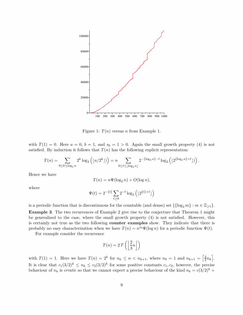
Figure 1: T (n) versus n from Example 1.
with T (1) = 0. Here a = 0, b = 1, and s0 = 1 > 0. Again the small growth property (4) is notsatisfied. By induction it follows that T (n) has the following explicit representation:
T (n) =∑
0≤k≤log2 n
2k log2
(⌊n/2k⌋)
)= n
∑
0≤ℓ≤⌊log2 n⌋2−{log2 n}−ℓ log2
(⌊2{log2 n}+ℓ⌋)
).
Hence we haveT (n) = nΨ(log2 n) + O(log n),
whereΨ(t) = 2−{t}∑
ℓ≥0
2−ℓ log2
(⌊2{t}+ℓ⌋
)
is a periodic function that is discontinuous for the countable (and dense) set {{log2 m} : m ∈ Z≥1}.
Example 3. The two recurrences of Example 2 give rise to the conjecture that Theorem 1 mightbe generalized to the case, where the small growth property (4) is not satisfied. However, thisis certainly not true as the two following counter examples show. They indicate that there isprobably no easy characterization when we have T (n) ∼ ns0Ψ(log n) for a periodic function Ψ(t).
For example consider the recurrence
T (n) = 2 T
(⌊2
3n
⌋)
with T (1) = 1. Here we have T (n) = 2k for nk ≤ n < nk+1, where n0 = 1 and nk+1 =⌈
32nk
⌉.
It is clear that c1(3/2)k ≤ nk ≤ c2(3/2)k for some positive constants c1, c2, however, the precisebehaviour of nk is erratic so that we cannot expect a precise behaviour of the kind nk = c(3/2)k +
9
O(1) and consequently not a representation of the form T (n) ∼ ns0Ψ(log n), since the jumps fromT (nk − 1) to T (nk) cannot be covered with the help of a single function Ψ(t).
Next consider the recurrence
T (n) = 2 T
(⌊n + 2
√n + 1
2
⌋)(n ≥ 6)
with T (n) = 1 for 1 ≤ n ≤ 5. Here we have (again) T (n) = 2k for nk ≤ n < nk+1, where n1 = 6 andnk+1 = ⌈2nk +1−2
√2nk⌉. It follows that nk is asymptotically of the form nk = c12k −c22k/2 +O(1)
(for certain positive constants c1, c2). Consequently it is again not possible to represent T (n)asymptotically as T (n) ∼ nΨ(log n).
Example 4. The recurrence
T (n) = T (⌊n/2⌋) + 2 T (⌈n/2⌉) + n
is related to the Karatsuba algorithm [22, 23]. Here we have s0 = log(1/3)/ log(1/2) = 1.5849 . . .and s0 > a = 1. Furthermore, since m = 1, we are in the rationally related case. Here the smallgrowth condition (4) is satisfied so that we can apply Theorem 1 to obtain
T (n) = Ψ(log n) nlog 3log 2 · (1 + o(1)) (n → ∞)
with some continuous periodic function Ψ(t).In a similar manner, the Strassen algorithm [7, 30] for matrix multiplications results in the
following recurrenceT (n) = T (⌊n/2⌋) + 6 T (⌈n/2⌉) + n2.
Here we have m = 1, s0 = log 7/ log 2 ≈ 2.81 and a = 2, and again we get an representation of theform
T (n) = Ψ(log n) nlog 7log 2 · (1 + o(1)) (n → ∞)
with some periodic function Ψ(t).
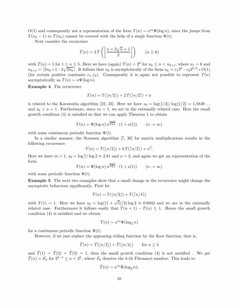
Example 5. The next two examples show that a small change in the recurrence might change theasymptotic behaviour significantly. First let
T (n) = T (⌊n/2⌋) + T (⌈n/4⌉)
with T (1) = 1. Here we have s0 = log((1 +√
5)/2) log 2 ≈ 0.6942 and we are in the rationallyrelated case. Furthermore it follows easily that T (n + 1) − T (n) ≤ 1. Hence the small growthcondition (4) is satisfied and we obtain
T (n) ∼ ns0Ψ(log2 n)
for a continuous periodic function Ψ(t).However, if we just replace the appearing ceiling function by the floor function, that is,
T (n) = T (⌊n/2⌋) + T (⌊n/4⌋) for n ≥ 4
and T (1) = T (2) = T (3) = 1, then the small growth condition (4) is not satisfied . We getT (n) = Fk for 2k−1 ≤ n < 2k, where Fk denotes the k-th Fibonacci number. This leads to
T (n) ∼ ns0Ψ(log2 n),
10
(a) (b)
Figure 2: Illustration to Example 5: (a) recurrence T (n) = T (⌊n/2⌋) + T (⌈n/4⌉), (b) recurrenceT (n) = T (⌊n/2⌋) + T (⌊n/2⌋).
where Ψ(t) = ((1 +√
5)/2)1−{t}/√
5 is discontinuous for t = 0; see also Figure 2.
Example 6. The recurrences
T (n) = T (⌊n/2⌋) + T (⌈n/2⌉) + n − 1,
Y (n) = Y (⌊n/2⌋) + Y (⌈n/2⌉) + ⌊n/2⌋,
U(n) = U(⌊n/2⌋) + U(⌈n/2⌉) + n − ⌊n/2⌋⌈n/2⌉ + 1
+⌈n/2⌉
⌊n/2⌋ + 1⌊n/2⌋
are related to Mergesort (see [13]). For all three recurrences we have a = s0 = 1 and we are(again) in the rationally related case. Here it is immediate to derive a-priori bounds of the formT (n + 1) − T (n) = O(log n) (and corresponding ones for Y (n) and U(n)).
Hence, we obtain asymptotic expansions of the form
C n log n + nΨ(log n) + o(n) (n → ∞),
where C = 1/ log 2 for T (n) and U(n) and C = 1/(2 log 2) for Y (n), and Ψ(t) is a continuousperiodic function.
Example 7. Consider nowT (n) = T (⌊n/2⌋) + log n.
Here we have a = s0 = 0 and consequently, according to case (ii) we have
T (n) =1
2 log 2(log n)2 + O(log n).
11
Example 8. Next consider the recurrence
T (n) = 2 T (⌊n/2⌋) +8
9T (⌊3n/4⌋) +
n2
log n.
Here a = s0 = 2. Hence, by the extended case (ii) (described in Remark 2) we have
T (n) =2
log 2 + log(4/3)n2log log n + O(n2/ log n).
Example 9. The solution of the recurrence
T (n) =1
3T
(⌊n
3+
1
2
⌋)+
2
3T
(⌈2n
3− 1
2
⌉)+ 1
with initial value T (1) = 0 is asymptotically given by
T (n) =1
Hlog n + C + o(1),
with H = 13 log 3 + 2
3 log 32 ≈ 0.6365 and some constant C. By Remark 5, we are in the irrationally
related case. With the help of Theorem 3 we can compute C ≈ −0.0813. Its precise form isC = −α/H, where
α =∑
m≥1
T (m + 2) − T (m + 1)
3
(log
⌈3m +
5
2
⌉− log(3m)
)
+ 2∑
m≥1
T (m + 2) − T (m + 1)
3
(log
⌊3
2m +
5
4
⌋− log(
3m
2)
)
+log 3
3− H −
13 log2 3 + 2
3 log2 32
2H≈ 0.0518.
We will use this example for computing the redundancy of the binary Boncelet code with p = 1/3in Section 4.
Example 10. Let s2(k) denote the binary sum-of-digits function of a non-negative integer k andlet T (n) =
∑k<n s2(k) the partial sums. Then T (n) satisfies the recurrence
T (n) = T (⌊n/2⌋) + T (⌈n/2⌉) + ⌊n/2⌋
and T (1) = 0. It is a well known fact (originally due to Delange [9]) that T (n) is given by
T (n) =1
2n log2 n + nΨ(log2 n),
where Ψ(t) a periodic function that is even continuous. There are several different representationsfor Ψ(t). For example we have
Ψ(t) = 2−{t}∑
ℓ≥0
2−ℓg(2ℓ+{t}
)+
1 − {x}2
,
12
where
g(t) =
∫ t
0
(⌊2{s/2}⌋ − 1
2
)ds.
Example 11. The recurrence
T (n) =1
4T (⌊n/2⌋) +
1
4T (⌈n/2⌉) +
1
n
is not covered by Theorem 1 since an is decreasing. Hence, T (n) is not increasing, either. However,we can adapt the proof methods of Theorem 1. Formally we have a = s0 = −1 < 0 and, sincem = 1, we are in the rationally related case. It follows that
Tn =1
log 2
log n
n+
Ψ(log n)
n+ o
(1
n
)
with a periodic function Ψ(t).
3 Dirichlet Series and Discrete Divide and Conquer Recurrences
In this section we present the full version of our theorem concerning the precise asymptotic behaviorof discrete divide and conquer recurrence.
3.1 Divide and Conquer Recurrence
Let us recall the general form of divide and conquer recurrences that we will analyze. For m ≥ 1,let b1, . . . , bm and b1, . . . , bm be positive real numbers and hj(x) and hj(x) non-decreasing positivefunctions with hj(x) = pjx + O(x1−δ) and hj(x) = pjx + O(x1−δ) for some positive numbers pj < 1and some δ > 0 (for 1 ≤ j ≤ m). We consider a (general) divide and conquer recurrence: givenT (0) ≤ T (1) for n ≥ 2 we set
T (n) = an +m∑
j=1
bjT (⌊hj(x)⌋) +m∑
j=1
bjT(⌈
hj(x)⌉)
(n ≥ 2), (10)
= an +m∑
j=1
bjT(⌊
pjx + O(x1−δ)⌋)
+m∑
j=1
bjT(⌈
pjx + O(x1−δ)⌉)
where (an)n≥2 is a known non-negative and non-decreasing sequence. We also assume that hj(n) < nand hj(n) ≤ n − 1 (for n ≥ 2 and 1 ≤ j ≤ m) so that the recurrence is well defined. It follows byinduction that T (n) is nondecreasing, too. In order to solve recurrence (10), we use Dirichlet series[3, 31]. In fact, in the proof presented in Section 5 we make use of the following Dirichlet series
T (s) =∞∑
n=1
T (n + 2) − T (n + 1)
ns(11)
from which we can calculate∑n−2
i=1 (T (i + 2) − T (i + 1)) = T (n) − T (2).For an asymptotic solution of recurrence (10), we will make some assumptions regarding the
Dirichlet series of the known sequence an. We postulate that the abscissa of absolute convergenceσa of the Dirichlet series
A(s) =∞∑
n=1
an+2 − an+1
ns(12)
13
is finite (or −∞), that is, A(s) represents an analytic function for ℜ(s) > σa. For example, if weknow that an is non-decreasing and
an = O(na(log n)b)
for some real number a and b, then A(s) converges (absolutely) for ℜ(s) > a. In particular, wehave σa ≤ a.
Analytically, these observations follow from the fact, proved in Section 5, that the Dirichletseries T (s) can be expressed as
T (s) =A(s) + B(s)
1 −∑mj=1(bj + bj) ps
j
(13)
for some analytic function B(s) and A(s) defined in (12). For the asymptotic analysis, we appealto the Tauberian theorem by Wiener-Ikehara and an analysis based on the Mellin-Perron formula(see Appendix B and Section 5.3). Both approaches rely on the singular behavior of T (s). By theMellin-Perron formula, we shall observe that
T (n) = T (2) +1
2πi
∫ c+i∞
c−i∞T (s)
(n − 32 )s
sds. (14)
Hence, the asymptotic behavior of T (n) depends on the singular behavior of A(s), on the singularityat s = 0, and on the roots of the denominator in (13), that is, roots of the characteristic equation
m∑
j=1
(bj + bj) psj = 1. (15)
We denote by s0 the unique real solution of this equation.A master theorem has usually three (major) parts. In the first case the (asymptotic) behavior
of an dominates the asymptotics of T (n), in the second case, there is an interaction between theinternal structure of the recurrence and the sequence an (resonance), and in the third case thebehavior of the solution is driven by the recurrence and does not depend on an; see the three casesof Theorem 1. This also corresponds to an interplay between the poles s = 0, s = σa and s0 thatdetermines the asymptotic behavior as illustrated in Figure 3. In fact, the pole of the largest valuedictates asymptotics and determines the leading term.
We will handle these cases separately. If s0 < σa or if s0 = σa (that is, we are in the first twocases) we have to assume some regularity properties about the sequence an in order to cope withthe asymptotics of T (n). We assume that A(s) has a certain extension to a region that containsthe line ℜ(s) = σa with a pole-like singularity at s = σa. To be more precise, we will assume thatthere exist functions F (s), g0(s), . . . , gJ(s) that are analytic in a region that contains the half planeℜ(s) ≥ σa such that
A(s) = g0(s)
(log 1
s−σa
)β0
(s − σa)α0+
J∑
j=1
gj(s)
(log 1
s−σa
)βj
(s − σa)αj+ F (s), (16)
where g0(σa) 6= 0, βj are non-negative integers, α0 is real, and α1, . . . , αJ are complex numberswith ℜ(αj) < α0 (1 ≤ j ≤ J), and β0 is non-negative if α0 is contained in the set {0, −1, −2, . . .}.
14
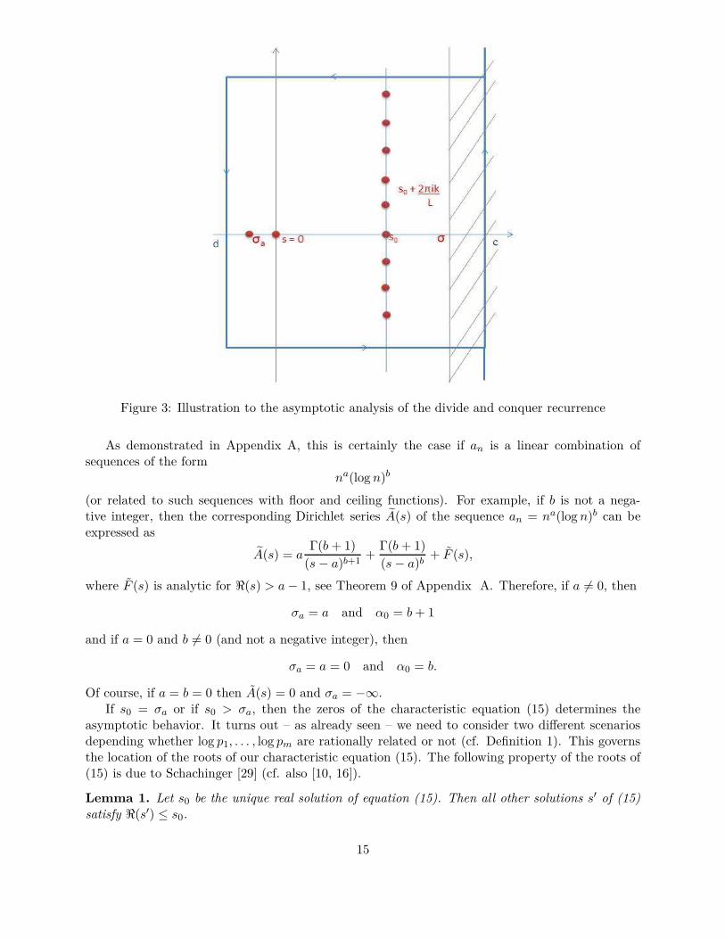
Figure 3: Illustration to the asymptotic analysis of the divide and conquer recurrence
As demonstrated in Appendix A, this is certainly the case if an is a linear combination ofsequences of the form
na(log n)b
(or related to such sequences with floor and ceiling functions). For example, if b is not a nega-tive integer, then the corresponding Dirichlet series A(s) of the sequence an = na(log n)b can beexpressed as
A(s) = aΓ(b + 1)
(s − a)b+1+
Γ(b + 1)
(s − a)b+ F (s),
where F (s) is analytic for ℜ(s) > a − 1, see Theorem 9 of Appendix A. Therefore, if a 6= 0, then
σa = a and α0 = b + 1
and if a = 0 and b 6= 0 (and not a negative integer), then
σa = a = 0 and α0 = b.
Of course, if a = b = 0 then A(s) = 0 and σa = −∞.If s0 = σa or if s0 > σa, then the zeros of the characteristic equation (15) determines the
asymptotic behavior. It turns out – as already seen – we need to consider two different scenariosdepending whether log p1, . . . , log pm are rationally related or not (cf. Definition 1). This governsthe location of the roots of our characteristic equation (15). The following property of the roots of(15) is due to Schachinger [29] (cf. also [10, 16]).
Lemma 1. Let s0 be the unique real solution of equation (15). Then all other solutions s′ of (15)satisfy ℜ(s′) ≤ s0.
15
(i) If log p1, . . . , log pm are irrationally related, then s0 is the only solution of (15) on ℜ(s) = s0.(ii) If log p1, . . . , log pm are rationally related, then there are infinitely many solutions sk, k ∈ Z,with ℜ(sk) = s0 which are given by
sk = s0 + k2πi
L(k ∈ Z),
where L > 0 is the largest real number such that log pj are all integer multiples of L. Furthermore,there exists δ > 0 such that all remaining solutions of (15) satisfy ℜ(s) ≤ s0 − δ.
3.2 General Discrete Master Theorem
We are now ready to formulate our main results regarding the asymptotic solutions of discrete divideand conquer recurrences. Note that the irrational case is easier to handle whereas the rational caseneeds additional assumptions on the Dirichlet series. Nevertheless these assumptions are usuallyeasy to establish in practice.
As discussed, our Discrete Master Theorem shows that for sequences an of practical importancesuch as
an = na(log n)b
the solution T (n) of the divide and conquer recurrence grows as
T (n) ∼ C na′
(log n)b′
(log log n)c′
(17)
with a′ = max{a, s0}) when log p1, . . . , log pm are irrationally related. For rationally related log p1,. . . , log pm, it is either of the form (17) or (if s0 > a) there appears an oscillation in the form of
T (n) ∼ Ψ(log n) ns0 (18)
with a continuous periodic function Ψ(t). The proof of the following general result will be given inSection 5.
Theorem 2 (Discrete Master Theorem – Full Version). Let T (n) be the divide and conquerrecurrence defined in (10) such that:
(A1) bj and bj are non-negative with bj + bj > 0,
(A2) hj(x) and hj(x) are increasing and non-negative functions such that hj(x) = pjx + O(x1−δ)and hj(x) = pjx + O(x1−δ) for positive pj < 1 and δ > 0, with hj(2) < 2, hj(2) ≤ 1,
(A3) the sequence (an)n≥2 is non-negative and non-decreasing.
(A4) Let σa denote the abscissa of absolute convergence of the Dirichlet series A(s) and s0 bethe real root of (15). If σa ≥ s0 ≥ 0 assume further that A(s) has a representation of theform (16), where F (s), g0(s), . . . , gJ (s) are analytic in a region that contains the half planeℜ(s) ≥ σa with g0(σa) 6= 0, α0 is real and ℜ(αj) < α0 (1 ≤ j ≤ J).
16
(i) If log p1, . . . , log pm are irrationally related, then as n → ∞
T (n) =
C1 + o(1) if σa < 0 and s0 < 0,C2 log n + C ′
2 + o(1) if σa < s0 and s0 = 0,C3(log n)α0+1(log log n)β0−I · (1 + o(1)) if σa = s0 = 0,C4 ns0 · (1 + o(1)) if σa < s0 and s0 > 0,C5ns0(log n)α0(log log n)β0−I · (1 + o(1)) if σa = s0 > 0,C6 (log n)α0(log log n)β0−I(1 + o(1)) if σa = 0 and s0 < 0,C7 nσa(log n)α0−1(log log n)β0−I · (1 + o(1)) if σa > s0 and σa > 0,
(19)
with positive real constants C1, C2, C3, C4, C5, C6, C7, where in particular if α0 /∈ {0, −1, −2, . . .} wehave I = 0. We only have I = 1 if α0 ∈ {0, −1, −2, . . .}, β0 > 0 and if in the corresponding casesof (19) we have
σa = s0 = 0 and α0 ≤ −2,σa = s0 > 0 and α0 ≤ −1,if σa = 0, s0 < 0, and α0 ≤ −1, orσa > s0 and σa > 0.
(ii) If log p1, . . . , log pm are rationally related and if in the case s0 = σa the Fourier series, with Ldefined in Lemma 1(ii),
∑
k∈Z\{0}
A(s0 + 2πik/L)
s0 + 2πik/Le2πikx/L (20)
is convergent for x ∈ R and represents an integrable function, then T (n) behaves as in the irra-tionally related case with the following two exceptions:
T (n) =
{C2 log n + Ψ2(log n) + O(n−η′
) if σa < s0 and s0 = 0,Ψ4(log n) ns0 + O(ns0−η′
) if σa < s0 and s0 > 0,(21)
where C2 and Ψ4(t) are positive and Ψ2(t), Ψ4(t) are continuous periodic functions with period Land η′ > 0, provided that the small growth condition
T (n + 1) − T (n) = O(ns0−η) (22)
holds for some η > 1 − δ.
Remark 6. We should point out that the periodic functions Ψ2(t) and Ψ4(t) that appear in thesecond part of Theorem 2 have building blocks of the form
λ−t/L∑
n≥1
Bnλ⌊ t−log n
L ⌋+1
λ − 1
for some λ > 1 and a sequence Bn such that the series∑
n≥1 Bnλ−(log n)/L is absolutely convergent.This representation suggests that the periodic functions should have countably many discontinu-ities and, thus, should not have absolutely convergent Fourier series. Nevertheless the small growthcondition (22) ensures that the final periodic function is actually continuous (see Lemma 4), how-ever, this property is not immediate. Actually we can expect Hölder continuous functions, that is|Ψ(s) − Ψ(t)| ≤ C|s − t|η for some η > 0 and absolutely convergent Fourier series, see [17].
17
Remark 7. The condition (20) for A(s) looks artificial. However, it is really needed in the proofin order to control the polar singularities of T (s) at sk, k ∈ Z \ {0}. Nevertheless it is no realrestriction in practice. As shown in Appendix A the condition (20) is satisfied for sequences of theform an = na(log n)b.
We now briefly show how Theorem 1 can be deduced from Theorem 2 which we prove inSection 5.
Case a > s0:We recall that if an = Cna(log n)b, then we have σa = a if a or b are different from zero andσa = −∞ if a = b = 0. Suppose that we are in the first case. By Theorems 9 and 10 of AppendixA the Dirichlet series A(s) satisfies the assumptions of Theorem 2. Recall that α0 = b + 1 and thatβ0 = I = 0. Consequently the last case of (19) applies and we obtain the asymptotic leading termfor T (n) ∼ C ′na(log n)b. The constant C ′ can be either determined from the proof of Theorem 2or more directly by inserting C ′na(log n)b into the recurrence and comparing coefficients – we leavethe easy details to the reader.
In order to obtain the remainder term we follow Remark 1. We set T (n) = C ′na(log n)b + S(n)and using the relation
(pjn + O(n1−δ)
)a (log(pjn + O(n1−δ)
)b= na(log n)bpa
j + O(na(log n)b−1
)
we obtain (if b > 0) a recurrence for S(n) of the form
S(n) =m∑
j=1
bjS (⌊hj(n)⌋) +m∑
j=1
bjS(⌈
hj(n)⌉)
+ O(na(log n)b−1
).
Hence by the Akra-Bazzi theorem it follows that S(n) = O(na(log n)b−1
), too. If b = 0, then the
error term is replaced by O(na−δ) and we get even a better estimate for S(n).Finally if a = b = 0 and s0 < 0, then we are in the first case of Theorem 2 and we observe
that T (n) = C ′ + o(1), where C ′ = C/(1 −∑m
j=1(bj + bj)). By setting T (n) = C ′ + S(n) we get a
homogeneous recurrence for S(n) and the Akra-Bazzi theorem proves S(n) = O(ns0).
Case a = s0:If a > 0 or b > 0, then σa = a. If a > 0, then we apply the fifth case of Theorem 2 (with α0 = b + 1and β0 = I = 0) and obtain T (n) ∼ C ′′na(log n)b+1. As in case (i) we obtain C ′′ explicitly and alsothe error term with a bootstrapping procedure.
If a = 0 and b > 0, then we have σa = s0 = 0 and α0 = b. Consequently the third case ofTheorem 2 applies. Again the constant as well the error term are derived as above.
Case a < s0:Observe that a < s0 implies σa < s0. Consequently we can apply the fourth case of Theorem 2and obtain T (n) ∼ C ′′′ns0 in the irrationally related case and T (n) ∼ Ψ(log n)ns0 in the rationallyrelated case.
Finally we mention that the extensions of Theorem 1 discussed in Remarks 2–4 are also coveredby Theorem 2. We leave the details to the reader.
18
4 Boncelet’s Arithmetic Coding Algorithm
We present a novel application of our analytic approach to discrete divide and conquer recurrencesby computing the redundancy of a practical variable-to-fixed compression algorithm due to Bon-celet [4]. To recall, a variable-to-fixed length encoder partitions the source string, say over anm-ary alphabet A, into a concatenation of variable-length phrases. Each phrase belongs to a givendictionary of source strings. A uniquely parsable dictionary is represented by a complete parsingtree, i.e., a tree in which every internal node has all m children nodes. The dictionary entriescorrespond to the leaves of the associated parsing tree. The encoder represents each parsed stringby the fixed length binary code word corresponding to its dictionary entry. There are several wellknown variable-to-fixed algorithms; e.g., Tunstall and Khodak schemes (cf. [10, 21, 32]). Boncelet’salgorithm, described next, is a practical and computationally fast algorithm that is coming intouse. Therefore, we compare its redundancy to the (asymptotically) optimal Tunstall’s algorithm.
Boncelet describes his algorithm in terms of a parsing tree. For fixed n (representing thenumber of leaves in the parsing tree and hence also the number of distinct phrases), the algorithmin each step creates two subtrees of predetermined number of leaves (phrases). Thus at the root,
n is split into two subtrees with the number of leaves, respectively, equal to n1 =⌊p1n + 1
2
⌋and
n2 =⌊p2n + 1
2
⌋. This continues recursively until only 1 or 2 leaves are left. Note that this splitting
procedure does not assure that n1 + n2 = n. For example if p1 = 38 and p2 = 5
8 , then n = 4would be split into n1 = 2 and n2 = 3. Therefore, we propose to modify the splitting as followsn1 = ⌊p1n + δ⌋ and n2 = ⌈p2n − δ⌉ for some δ ∈ (0, 1) that satisfies 2p1 + δ < 2.
Let {v1, . . . vn} denote phrases of the Boncelet code that correspond to the paths from the rootto leaves of the parsing tree, and let ℓ(v1), . . . , ℓ(vn) be the corresponding phrase lengths. Observethat while the parsing tree in the Boncelet’s algorithm is fixed, a randomly generated sequence ispartitioned into random length phrases. Therefore, one can talk about the probabilities of phrasesdenoted as P (v1), . . . , P (vn). Here we restrict the analysis to a binary alphabet and denote theprobabilities by p := p1 and q := p2 = 1 − p.
For sequences generated by a binary memoryless source, we aim at understanding the proba-bilistic behavior of the phrase length that we denote as Dn. Its probability generating function isdefined as
C(n, y) = E[yDn ]
which can also be represented as
C(n, y) =n∑
j=1
P (vj)yℓ(vj).
The Boncelet’s splitting procedure leads to the following recurrence on C(n, y) for n ≥ 2
C(n, y) = p y C (⌊pn + δ⌋ , y) + q y C (⌈qn − δ⌉ , y) (23)
with initial conditions C(0, y) = 0 and C(1, y) = 1.Next let d(n) denote the average phrase length
E[Dn] := d(n) =n∑
j=1
P (vj) ℓ(vj)
19

which is also given by d(n) = C ′(n, 1) (where the derivative is taken with respect to y) and satisfiesthe recurrence
d(n) = 1 + p1d (⌊p1n + δ⌋) + p2d (⌈p2n − δ⌉) (24)
with d(0) = d(1) = 0. This recurrence falls exactly under our general divide and conquer recurrence,hence Theorem 2 applies.
Theorem 3. Consider a binary memoryless source with positive probabilities p1 = p and p2 = qand the entropy rate H = p log(1/p) + q log(1/q). Let d(n) = E[Dn] denote the expected phraselength of the binary Boncelet code.(i) If the ratio (log p)/(log q) is irrational, then
d(n) =1
Hlog n − α
H+ o(1), (25)
where
α = E′(0) − G′(0) − H − H2
2H, (26)
H2 = p log2 p + q log2 q, and E′(0) and G′(0) are the derivatives at s = 0 of the Dirichlet seriesdefined in (32) of Section 5 and Remark 3 of Section 2.(ii) If (log p)/(log q) is rational, then
d(n) =1
Hlog n − α + Ψ(log n)
H+ O(n−η), (27)
where Ψ(t) is a periodic function and η > 0.
For practical data compression algorithms, it is important to achieve low redundancy definedas the excess of the code length over the optimal code length nH. For variable-to-fixed codes, theaverage redundancy is expressed as [10, 28]
Rn =log n
E[Dn]− H =
log n
d(n)− H
since every phrase of average length d(n) requires log n bits to point to a dictionary entry. Ourprevious results imply immediately the following corollary.
Corollary 1. Let Rn denote the redundancy of the binary Boncelet code with positive probabilitiesp1 = p and p2 = q.(i) If the ratio (log p)/(log q) is irrational, then
Rn =Hα
log n+ o
(1
log n
)(28)
with α defined in (26).(ii) If (log p)/(log q) is rational, then
Rn =H(α + Ψ(log n))
log n+ o
(1
log n
)(29)
where Ψ(t) is a periodic function.
20
We should compare the redundancy of Boncelet’s algorithm to the asymptotically optimalTunstall algorithm. From [10, 28] we know that the redundancy of the Tunstall code is
RTn =
H
log n
(− log H − H2
2H
)+ o
(1
log n
)
(provided that (log p)/(log q) is irrational; in the rational case there is also a periodic term in theleading asymptotics). This should be compared to the redundancy of the Boncelet algorithm.
Example. Consider p = 1/3 and q = 2/3. Then the recurrence for d(n) is precisely the sameas that of Example 9. Consequently α ≈ 0.0518 while for the Tunstall code the correspondingconstant is equal to − log H − H2
2H ≈ 0.0496.
5 Analysis and Asymptotics
We prove here a general asymptotic solution of the divide and conquer recurrence (cf. Theorem 2).We first derive the appropriate Dirichlet series and apply Tauberian theorems for the irrationallyrelated case, then discuss the Perron-Mellin formula, and finally finish the proof of Theorem 2 forthe rationally related case.
5.1 Dirichlet Series
As discussed in the previous section, the proof makes use of the Dirichlet series
T (s) =∞∑
n=1
T (n + 2) − T (n + 1)
ns,
where we apply Tauberian theorems and the Mellin-Perron formula to obtain asymptotics for T (n)from singularities of T (s).
By partial summation and using a-priori upper bounds for the sequence T (n), it follows thatT (s) converges (absolutely) for s ∈ C with ℜ(s) > max{s0, σa, 0}, where s0 is the real solution ofthe equation (15), and σa is the abscissa of absolute convergence of A(s).
Next we apply the recurrence relation (10) to T (s). To simplify our presentation, we assumethat bj = 0, that is, we consider only the floor function on the right hand side of the recurrence(10); those parts that contain the ceiling function can be handled in the same way. We thus obtain
T (s) = A(s) +m∑
j=1
bj
∞∑
n=1
T (⌊hj(n + 2)⌋) − T (⌊hj(n + 1)⌋)
ns.
For k ≥ 1 setnj(k) := max{n ≥ 1 : hj(n + 1) < k + 2}.
By definition it is clear that nj(k + 1) ≥ nj(k) and
nj(k) =n
pj+ O
(k1−δ
). (30)
21

Furthermore, by setting Gj(s) as in (6) of Remark 3 we obtain
∞∑
n=1
T (⌊hj(n + 2)⌋) − T (⌊hj(n + 1)⌋)
ns= Gj(s) +
∞∑
k=1
T (k + 2) − T (k + 1)
nj(k)s.
We now compare the last sum to psj T (s):
∞∑
k=1
T (k + 2) − T (k + 1)
nj(k)s=
∞∑
k=1
T (k + 2) − T (k + 1)
(k/pj)s
−∞∑
k=1
(T (k + 2) − T (k + 1))
(1
(k/pj)s− 1
nj(k)s
)
= psj T (s) − Ej(s),
where Ej(s) is defined in (7) of Remark 3. Defining
E(s) =m∑
j=1
bjEj(s) and G(s) =m∑
j=1
bjGj(s)
we finally obtain the relation
T (s) =A(s) + G(s) − E(s)
1 −∑mj=1 bj ps
j
. (31)
As mentioned above, (almost) the same procedure applies if some of the bj are positive, thatis, the ceiling function also appear in the recurrence equation. The only difference to (31) is thatwe arrive at a representation of the form
T (s) =A(s) + G(s) − E(s)
1 −∑mj=1(bj + bj) ps
j
, (32)
with a properly modified functions G(s) and E(s), however, they have the same analyticity prop-erties as in (31), compare also with Remark 3.
By our previous assumptions, we know the analytic behaviors of
A(s) and
1 −m∑
j=1
(bj + bj) psj
−1
:
A(s) has a pole-like singularity at s = σa (if σa ≥ s0) and a proper continuation to a complexdomain that contains the (punctuated) line ℜ(s) = σa, s 6= σa. On the other hand,
1
1 −∑mj=1(bj + bj) ps
j
has a polar singularity at s = s0 (and infinitely many other poles on the line ℜ(s) = s0 if thenumbers log pj are rationally related), and also a meromorphic continuation to a complex domain
22

that contains the line ℜ(s) = s0. Furthermore, G(s) is an entire function. It suffices to discussEj(s). First observe that (30) implies
1
(k/pj)s− 1
nj(k)s= O
(1
(k/pj)ℜ(s)+δ
).
By partial summation (and by using again the a-priori estimates), it follows immediately that theseries ∞∑
k=1
(T (k + 2) − T (k + 1))1
(k/pj)ℜ(s)+δ
converges for ℜ(s) > max{s0, σa, 0}−δ. Since T (n) is an increasing sequence, this implies (absolute)convergence of the series Ej(s), just representing an analytic function in this region, too.
In order to recover (asymptotically) T (n) from T (s) we need to apply several different techniquesdiscussed in the next subsection. The main analytic tools are Tauberian theorems (of Wiener-Ikehara which is discussed in detail in Appendix B) and the Mellin-Perron formula (Theorem 4).
5.2 Tauberian Theorems
We are now ready to prove several parts of Theorem 2 with the help of Tauberian theorems ofWiener-Ikehara type (see Appendix B). We recall that such theorems apply in general to theso-called Mellin-Stieltjes transform
∫ ∞
1−v−s dc(v) = s
∫ ∞
1c(v)v−s−1 dv
of a non-negative and non-decreasing function c(v). If c(n) is a sequence of non-negative numbers,then the Dirichlet series C(s) =
∑n≥1 c(n)n−s is just the Mellin-Stieltjes transform of the function
c(v) =∑
n≤v c(n):
C(s) =∑
n≥1
c(n)n−s =
∫ ∞
1−v−s dc(v) = s
∫ ∞
1c(v)v−s−1 dv.
Informally, a Tauberian theorem is a correspondence between the singular behavior of 1s C(s) and
the asymptotic behavior of c(v). In the context of Tauberian theorems of Wiener-Ikehara type oneassumes that C(s) continues analytically to a proper region, has only one (real) singularity s0 onthe critical line ℜ(s) = s0, and the singularity is of special type (for example a polar or algebraicsingularity, see Appendix B).
We recall that T (s) is the Dirichlet series of the sequence c(n) = T (n + 2) − T (n + 1). Hence
T (n) = c(n − 2) + T (2).
Consequently, if we know the asymptotic behavior of c(v) we also find that of T (n). Notice thatT (s) is given by (32). Hence the dominant singularity of 1
s T (s) is either zero, or induced by the
singular behavior of A(s), or induced by the zeros of the denominator
1 −m∑
j=1
(bj + bj)psj .
23
Here it is essential to assume that the log pj are irrationally related. Precisely in this case thedenominator has only the real zero s0 on the line ℜ(s) = s0. Hence Tauberian theorems can beapplied in the irrationally related case if s0 ≥ σa. (For the rational case we will apply a differentapproach to cover the case s0 ≥ σa.)
Our conclusions for the proof of the first part of Theorem 2 are summarized as follows:
1. σa < 0 and s0 < 0:This is indeed a trivial case, since the dominant singularity is at s = 0 and the series T (s)converges for s = 0:
T (0) =∑
n≥1
(T (n + 2) − T (n + 1)),
henceT (n) = C1 + o(1),
where C1 = T (2) + T (0).
2. σa < s0 and s0 = 0:We can apply directly a proper version of the Wiener-Ikehara theorem (Theorem 12 of Ap-pendix B) that proves
T (n) = C2 log n · (1 + o(1)).
Observe, that s = 0 is a double pole of 1s T (s) that induces the log n-term in the asymptotic
expansion. Note that this does not prove the full version that is stated in Theorem 2. Byapplying Theorem 5 of the next subsection (that is based on a more refined analysis) we alsoarrive at an asymptotic expansion of the form
T (n) = C2 log n + C ′2 + o(1).
3. σa = s0 = 0:In this case, we obtain at s = 0 the dominant singular term of 1
s T (s) that is given by
C(log(1/s))β0
sα0+2with C =
−g0(0)∑m
j=1(bj + bj) log pj
Hence, an application of Theorem 13 of Appendix B provides the asymptotic leading termfor T (n). Recall that we have to handle separately the case when α0 is contained in the set{−2, −3, . . .} (and β0 > 0). In this case, only logarithmic singularities remain.
4. σa < s0 and s0 > 0:Here the classical version of the Wiener-Ikehara theorem (Theorem 11 of Appendix B) applies.Note again that it is crucial that the denominator has only one pole on the line ℜ(s) = s0.
5. σa = s0 > 0:Here the function 1
s T (s) has the dominant singular term
C(log(1/(s − σa)))β0
(s − σa)α0+1
24

for some constant C > 0 (and there are no other singularities on the line ℜ(s) = s0). Thus, anapplication of Theorem 13 of Appendix B provides the asymptotic leading term for T (n). Ob-serve that we have to handle separately the case when α0 is contained in the set {−1, −2, . . .}(and β0 > 0).
6. σa = 0 and s0 < 0:The analysis of this case is very close to the previous one. The dominant singular term of1s T (s) is of the form
C(log(1/s))β0
sα0+1.
7. σa > s0 and σa > 0:In this case the singular behavior of A(s) dominates the asymptotic behavior of 1
s T (s). Anapplication of Theorem 13 of Appendix B provides the asymptotic leading term of T (n).
5.3 Mellin-Perron Formula
One disadvantage of the use of Tauberian theorems is that they provide (usually) only the asymp-totic leading term and no error terms. In order to provide error terms or second order terms one hasto use more refined methods. In the framework of Dirichlet series we can apply the Mellin-Perronformula that we recall next.
Below we shall use Iverson’s notation [[P ]] which is 1 if P is a true proposition and 0 else.
Theorem 4 (see [3]). For a sequence c(n) define the Dirichlet series
C(s) =∞∑
n=1
c(n)
ns
and assume that the abscissa of absolute convergence σa is finite or −∞. Then for all σ > σa andall x > 0
∑
n<x
c(n) +c(⌊x⌋)
2[[x ∈ Z]] = lim
T →∞1
2πi
∫ σ+iT
σ−iTC(s)
xs
sds.
Note that – similarly to the Tauberian theorems – the Mellin-Perron formula enables us toobtain precise information about the function c(v) =
∑n≤v c(n) if we know the behavior of 1
s C(s).In our context we have c(n) = T (n + 2) − T (n), that is,
T (n) = T (2) + limT →∞
1
2πi
∫ c+iT
c−iTT (s)
(n − 32)s
sds (33)
with
T (s) =∞∑
n=1
T (n + 2) − T (n + 1)
ns.
As a first application we apply the Mellin-Perron formula of Theorem 4 for Dirichlet series ofthe form
C(s) =∑
n≥1
c(n)n−s =B(s)
1 −∑mj=1 bjps
j
, (34)
25

where we assume that the log pj are not rationally related and where B(s) is analytic in a regionthat contains the real zero s0 of the denominator. This theorem can be also applied to the proofof some parts of Theorem 2; in particular for the (irrationally related) cases
if σa < 0 and s0 < 0,if σa < s0 and s0 = 0, andif σa < s0 and s0 > 0.
Note that Theorem 5 provides a second order term in the case σa < s0 = 0, see also Remark 9.
Theorem 5. Suppose that 0 < pj < 1, 1 ≤ j ≤ m, are given such that log pj, 1 ≤ j ≤ m, are notrationally related and let s0 denote the real solution of the equation
m∑
j=1
bjpsj = 1,
where bj > 0, 1 ≤ j ≤ m. Let C(s) =∑
n≥1 c(n)n−s be a Dirichlet series with non-negativecoefficients c(n) that has a representation of the form (34), that is,
C(s) =∑
n≥1
c(n)n−s =B(s)
1 −∑mj=1 bjps
j
where B(s) is an analytic function for ℜ(s) ≥ s0 − η for some η > 0 and satisfies B(s) = O(|s|α)in this region for some α < 1. Then
∑
n≤v
c(n) =
B(0)
1 −∑mj=1 bj
+ o(1) if s0 < 0,
B(0)
H(0)log v +
B′(0) + B(0)H2/H
H+ o(1) if s0 = 0,
B(s0)
s0H(s0)vs0 (1 + o(1)) if s0 > 0
,
where H(s) = −∑mj=1 bjps
j log pj with H = H(0), and H2(s) =∑m
j=1 bjpsj(log pj)
2 with H2 = H2(0).
We quickly check that Theorem 5 is applicable for T (s) in the above mentioned cases. SinceA(s) and G(s) are convergent Dirichlet series with non-negative coefficients that stay bounded forℜ(s) ≥ s0 −η, however, for E(s) we only get an estimate of the form E(s) = O(|s|α) for some α < 1(we leave the details to the reader). Thus, everything fits together.
Remark 8. Note that the case s0 < 0 is immediate since the series is convergent for s = 0.Furthermore, the case s0 > 0 is covered by the Wiener-Ikehara theorem. The case s0 = 0 is themost interesting case. Here the Wiener-Ikehara theorem provides only the asymptotic leading term.However, the assumptions of Theorem 5 are much stronger than those needed for the Wiener-Ikeharatheorem. Actually we can cover also multiple poles and obtain also corresponding (non-leading)terms in the asymptotic expansion. In order to present these kind of techniques we will considerthe cases s0 > 0 and s0 = 0 in the following proof.
26
Proof. We start with the case s0 > 0. We will use the Mellin-Perron formula of Theorem 4,however, we cannot use it directly, since there are convergence problems. Namely, if we shift theline of integration ℜ(s) > s0 to the left (to ℜ(s) = σ < s0) and collect residues we obtain (withZ = {s ∈ C :
∑mj=1 bjps
j = 1})
∑
n≤v
c(n) = limT →∞
∑
s′∈Z, ℜ(s′)>σ, |ℑ(s′)|<T
Res(C(s)vs
s, s = s′)
+1
2πilim
T →∞
∫ σ+iT
σ−iTC(s)
vs
sds
= limT →∞
∑
s′∈Z, ℜ(s′)>σ, |ℑ(s′)|<T
B(s′)vs′
s′H(s′)
+1
2πilim
T →∞
∫ σ+iT
σ−iT
B(s)
1 −∑mj=1 bjp
sj
vs
sds
provided that the series of residues converges and the limit T → ∞ of the last integral exists. Theproblem is that neither the series nor the integral above are necessarily absolutely convergent sincethe integrand is only of order 1/s. We have to introduce the auxiliary function
c1(v) =
∫ v
0
∑
n≤w
c(n)
dw
which is also given by
c1(v) =1
2πi
∫ c+i∞
c−i∞C(s)
vs+1
s(s + 1)ds =
1
2πi
∫ c+i∞
c−i∞
B(s)
1 −∑mj=1 bjps
j
· vs+1
s(s + 1)ds,
for c > s0. Note that there is no need to consider the limit T → ∞ in this case since theseries and the integral are now absolutely convergent. Hence, the above procedure works withoutany convergence problem. In order to make the presentation of our analysis slightly easier weadditionally assume that the region of analyticity of B(s) is large enough such that it covers allzeros in Z and also the point −1. We now shift the line of integration to ℜ(s) = σ < min{−1, s0}.Then we have to consider the (absolutely convergent) sum of residues
∑
s′∈Z,
Res
(C(s)
vs+1
s(s + 1), s = s′
)=∑
s′∈Z
B(s′)s′(s′ + 1)H(s′)
vs′+1,
the residues at s = 0 and s = −1:
B(0)
1 −∑mj=1 bj
v, − B(−1)
1 −∑mj=1 bjp−1
j
,
and the remaining (absolutely convergent) integral
1
2πi
∫ σ+i∞
σ−i∞C(s)
vs+1
s(s + 1)ds =
1
2πi
∫ σ+i∞
σ−i∞
B(s)
1 −∑mj=1 bjps
j
vs+1
s(s + 1)ds = O(v1+σ).
27
Thus, we obtain
c1(v) =B(s0)
s0(s0 + 1)H(s0)(1 + Q(log v))v1+s0 + O(v1+s0−η)
for some η > 0, where
Q(x) =∑
s′∈Z\{s0}
s0(s0 + 1)H(s0)B(s′)s′(s′ + 1)H(s′)B(s0)
ex(s′−s0).
It is easy to show that Q(x) → 0 as x → ∞ (cf. also [29, Lemma 4] and [31]). Indeed, supposethat ε > 0 is given. Then there exists S0 = S0(ε) > 0 such that
∑
s′∈Z, |s′|>S0
∣∣∣∣s0(s0 + 1)H(s0)B(s′)s′(s′ + 1)H(s′)B(s0)
∣∣∣∣ <ε
2.
Further, since ℜ(s′) < s0 for all s′ ∈ Z \ {s0}, and by the assumption of irrationality the zeros arenot on the critical line ℜ(s) = s0 (except the real one), it follows that there exists x0 = x0(ε) > 0with ∣∣∣∣∣∣
∑
s′∈Z\{s0}, |s′|≤S0
s0(s0 + 1)H(s0)B(s′)s′(s′ + 1)H(s′)B(s0)
ex(s′−s0)
∣∣∣∣∣∣<
ε
2
for x ≥ x0. Hence |Q(x)| < ε for x ≥ x0(ε).Note that we cannot obtain the rate of convergence for Q(x). This means that we just get
c1(v) =B(s0)
s0(s0 + 1)H(s0)· v1+s0 + o(v1+s0)
as v → ∞, where s′ with ℜ(s′) < s0 contribute to the error term. However, since,∑
n≤v c(n) ismonotonely increasing in v (by assumption) it also follows that
∑
n≤v
c(n) ∼ B(s0)
s0H(s0)vs0 ,
compare with the case s0 = 0 that we discuss next.Now suppose that s0 = 0 which means that C(s) has a double pole as s = 0. We can almost
use the same analysis as above and obtain the asymptotic expansion
c1(v) =B(0)
Hv log v +
B′(0) − B(0) + B(0)H2/H
Hv + o(v).
It is now an easy exercise to derive from this expansion the final result
∑
n≤v
c(n) =B(0)
Hlog v +
B′(0) + B(0)H2/H
H+ o(1) (35)
in the following way. For simplicity we write c1(v) = C1v log v + C2v + o(v). By the assumption
|c1(v) − C1v log v + C2v| ≤ εv
28

for v ≥ v0. Set v′ = ε1/2v, then by monotonicity we obtain (for v ≥ v0)
∑
n≤v
c(n) ≤ c1(v + v′) − c1(v)
v′ ≤ 1
v′(C1(v + v′) log(v + v′) + C2(v + v′)−
C1v log v − C2v) + ε2v + v′
v′
= C1 log(v + v′) + C2 + C1v
v′ log
(1 +
v′
v
)+ ε
2v + v′
v′
= C1 log v + C2 + C1 + O(ε1/2
),
where the O-constant is an absolute one. In a similar manner, we obtain the corresponding lower
bound (for v ≥ v0 + v1/20 ). Hence, it follows that
∣∣∣∣∣∣
∑
n≤v
c(n) − C1 log v − C1 − C2
∣∣∣∣∣∣≤ C ′ε1/2
for v ≥ v0 + v1/20 . This proves
∑n≤v c(n) = C1 log v + C1 + C2 + o(1) and consequently (35).
Remark 9. The advantage of the preceding proof is its flexibility. For example, we can apply theprocedure for multiple poles and are able to derive asymptotic expansions of the form
∑
n≤v
c(n) =K∑
j=0
Aj(log v)j
j!vs0 + o(vs0).
Furthermore we can derive asymptotic expansions that are uniform in an additional parameterwhen we have some control on the singularities in terms of the additional parameter. We will usethis generalization in the proof of the central limit theorem for the phrase lengths of the Bonceletcode (Theorem 7).
In principle it is also possible to obtain bounds for the error terms. However, they dependheavily on Diophantine approximation properties of the vector (log p1, . . . log pm), see [16].
5.4 The Rationally Related Case
Unfortunately, the previous method generally is not applicable when there are several poles (orinfinitely many poles) on the line ℜ(s) = s0. This means that we cannot use the above procedurewhen the log pj are rationally related. The reason is that it does not follow automatically that anasymptotic expansion of the form
c1(v) =
∫ v
0c(w) dw ∼ Ψ1(log v) · vs0+1
impliesc(v) ∼ Ψ(log v) · vs0
for certain periodic functions Ψ and Ψ1, even if c(v) is non-negative and non-decreasing.
29

Therefore we will apply an alternative approach which is – in some sense – more direct andapplies only in this case, but it proves a convergence result for c(v) of the form
c(v) =∑
n≤v
c(n) ∼ Ψ(log v) vs0 .
Suppose that log pj = −njL for coprime integers nj and a real number L > 0. Then theequation 1 =
∑mj=1 bjps
j with the only real solution s0 becomes an algebraic equation
1 −m∑
j=1
bjznj = 0 with z = e−Ls.
with a single (dominating) real root z0 = e−Ls0 . We can factor this polynomial as
1 −m∑
j=1
bjznj = (1 − eLs0z)P (z), P (e−Ls) 6= 0,
and obtain also a partial fraction decomposition of the form
1
1 −∑mj=1 bjznj
=1/P (e−Ls0)
1 − eLs0z+
Q(z)
P (z).
Therefore, to study (33) with C(s) as in (33) it is natural in this context to consider Mellin-Perronintegrals of the form
1
2πilim
T →∞
∫ c+iT
c−iT
B(s)
1 − e−Lsλ
xs
sds
for some complex number λ 6= 0 and a Dirichlet series B(s). The corresponding result is statedbelow in Theorem 6.
To derive asymptotics of the above integral (cf. Theorem 6 below) we need the following twolemmas. The first lemma (Lemma 2) is also the basis of the proof of the Mellin-Perron formula (cf.[3, 31]). For the reader’s convenience we provide a short proof of Lemma 2.
Lemma 2. Suppose that a and c are positive real numbers. Then∣∣∣∣∣
1
2πi
∫ c+iT
c−iTas ds
s− 1
∣∣∣∣∣ ≤ ac
πT log a(a > 1),
∣∣∣∣∣1
2πi
∫ c+iT
c−iTas ds
s
∣∣∣∣∣ ≤ ac
πT log(1/a)(0 < a < 1),
∣∣∣∣∣1
2πi
∫ c+iT
c−iTas ds
s− 1
2
∣∣∣∣∣ ≤ C
T(a = 1).
Proof. Suppose first that a > 1. By considering the contour integral of the function F (s) = as/saround the rectangle with vertices −A − iT, c − iT, c + iT, −A + iT and letting A → ∞ one directlyobtains the representation
1
2πi
∫ c+iT
c−iTas ds
s= Res(as/s; s = 0) +
1
2πi
∫ c
−∞
ax+iT
x + iTdx +
1
2πi
∫ c
−∞
ax−iT
x − iTdx.
30

Since ∣∣∣∣∣1
2πi
∫ c
−∞
ax±iT
x ± iTdx
∣∣∣∣∣ ≤ ac
πT log a
we directly obtain the bound in the case a > 1.The case 0 < a < 1 can be handled in the same way. And finally, in the case a = 1 the integral
can be explicitly calculated (and estimated).
Lemma 3. Suppose that L is a positive real number, λ a complex number different from 0 and 1,and c a real number with c > 1
L log |λ|. Then we have for all real numbers x > 1
1
2πilim
T →∞
∫ c+iT
c−iT
1
1 − e−Lsλ· xs
sds =
λ⌊ log xL ⌋+1 − 1
λ − 1− 1
2λ⌊ log x
L ⌋[[log x/L ∈ Z]]. (36)
Proof. By assumption we have |λe−Ls| < 1. Thus, by using a geometric series expansion we get forall x > 1 such that log x/L is not an integer
1
2πi
∫ c+iT
c−iT
1
1 − e−Lsλ· xs
sds =
∑
k≥0
λk 1
2πi
∫ c+iT
c−iT
(x
eLk
)s ds
s
=∑
k≤ log xL
λk + O
1
T
∑
k≥0
|λ|k(
xeLk
)c
∣∣∣log(
xeLk
)∣∣∣
=λ⌊ log x
L ⌋+1 − 1
λ − 1+ O
(1
T
xc
1 − 1eLc |λ|
).
In the second line above we use the first part of Lemma 2 replacing the integral by 1 plus the errorterm. Similarly we can proceed if log x/L is an integer which implies (36).
Theorem 6. Let L be a positive real number, λ be a non-zero complex number, and suppose that
B(s) =∑
n≥1
Bnn−s
is a Dirichlet series that is absolutely convergent for ℜ(s) > 1L log |λ| − η for some η > 0. Then
1
2πilim
T →∞
∫ c+iT
c−iT
B(s)
1 − e−Lsλ
xs
sds =
∑
n≥1
Bnλ⌊
log(x/n)L
⌋+1
λ − 1− 1
2
∑
n≥1
Bnλ⌊
log(x/n)L
⌋[[log(x/n)/L ∈ Z]]
(37)
+ O(x
1L
log |λ|−η)
.
if |λ| > 1, and
1
2πilim
T →∞
∫ c+iT
c−iT
B(s)
1 − e−Ls
xs
sds =
∑
n≥1
Bn
(⌊log(x/n)
L
⌋+ 1
)(38)
− 1
2
∑
n≥1
Bn[[log(x/n)/L ∈ Z]] + O(x−η) .
if λ = 1.
31
Proof. We split the integral into an infinite sum of integrals according to the series B(s) =∑n≥1 Bnn−s and apply (36) for each term by replacing x by x/n.
First assume that log(x/n)/L is not an integer for n ≥ 1. Hence, if x > neLk, then we have
1
2πi
∫ c+iT
c−iT
n−s
1 − e−Lsλ
xs
sds =
λ⌊
log(x/n)L
⌋+1 − 1
λ − 1+
O
1
T
∑
k≥0
|λ|k(
xeLkn
)c
∣∣∣log(
xeLkn
)∣∣∣
,
and if x < neLk, then we just have
1
2πi
∫ c+iT
c−iT
n−s
1 − e−Lsλ
xs
sds = O
1
T
∑
k≥0
|λ|k(
xeLkn
)c
∣∣∣log(
xeLkn
)∣∣∣
.
Further, for given x there are only finitely many pairs (k, n) with∣∣∣∣
x
eLkn− 1
∣∣∣∣ <1
2.
Hence, the series
∑
n≥1
∑
k≥0
Bn
|λ|k(
xeLkn
)c
∣∣∣log(
xeLkn
)∣∣∣
is convergent. Consequently, we find
1
2πilim
T →∞
∫ c+iT
c−iT
∑n≥1 Bnn−s
1 − e−Lsλ
xs
sds =
1
λ − 1
∑
n<x
Bn
(λ⌊
log(x/n)L
⌋+1 − 1
)+ O(1)
(and a similar expression if there are integers n ≥ 1 for which log(x/n)/L is an integer). Finally,since ∑
n<x
Bn = O(n
1L
log |λ|−η)
and ∑
n>x
Bnn− 1L
log |λ| = O(x−η)
it follows that
1
λ − 1
∑
n<x
Bn
(λ⌊
log(x/n)L
⌋+1 − 1
)=
1
λ − 1
∑
n≥1
Bn
(λ⌊
log(x/n)L
⌋+1)
+ O(n
1L
log |λ|−η)
(and similarly if there are integers n ≥ 1 for which log(x/n)/L is an integer). This proves (40).If λ = 1 we first observe that (36) rewrites to
1
2πilim
T →∞
∫ c+iT
c−iT
1
1 − e−Ls
xs
sds =
⌊log x
L
⌋+ 1 − 1
2[[log x/L ∈ Z]].
Now the proof of (38) is very similar to that of (40).
32
Remark 10. The representations (37) and (38) have nice interpretations. When |λ| > 1 set
Ψ(t) = λ−t/L∑
n≥1
Bnλ⌊ t−log n
L ⌋+1
λ − 1− λ−t/L
2
∑
n≥1
Bnλ⌊ t−log nL ⌋[[(t − log n)/L ∈ Z]]. (39)
Then Ψ(t) is a periodic function of bounded variation with period L, that has (usually) countablymany discontinuities for t = L{log n/L}, n ≥ 1 (where we recall {x} = x − ⌊x⌋ is the fractionalpart of x). We arrive at
1
2πilim
T →∞
∫ c+iT
c−iT
B(s)
1 − e−Lsλ
xs
sds = x
1L
log λ Ψ (log x) + O(x
1L
log |λ|−η)
.
Formally, this representation also follows by adding the residues of
B(s)/(1 − e−Lsλ)
at s = s0 + 2kπi/L (k ∈ Z) which are the zeros of 1− eLsλ = 0. This means the leading asymptoticfollows (in this case) from a formal residue calculus.
Furthermore, if we go back to the original problem, where we have to discuss a function of theform
B(s)
1 −∑mj=1 bjps
j
,
for log pj rationally related, then we have
1
2πilim
T →∞
∫ c+iT
c−iT
B(s)
1 −∑mj=1 bjp
sj
xs
sds = xs0 Ψ (log x) + O
(xs0−η) .
As mentioned above we split up the integral with the help of a partial fraction decomposition ofthe rational function
1
1 −∑mj=1 bjznj
.
The leading term can be handled directly with the help of Theorem 3. The remaining terms canuse again (36) and obtains (finally) a second error term of order O (xs0−η).
Remark 11. If λ = 1 then the situation is even simpler. Set
C =1
L
∑
n≥1
Bn
and
Ψ(t) =∑
n≥1
Bn
(−{
t − log n
L
}+ 1
)− 1
2
∑
n≥1
Bn[[(t − log n)/L ∈ Z]] − 1
L
∑
n≥1
Bn log n.
Then Ψ(t) is a periodic function with period L, that has (usually) countably many discontinuitiesfor t = L{log n/L}, n ≥ 1, and we have
1
2πilim
T →∞
∫ c+iT
c−iT
B(s)
1 − e−Ls
xs
sds = C log x + Ψ (log x) + O
(x−η) .
33
Hence, by applying the same partial fraction decomposition as above we also obtain (if s0 = 0 andif the log pj are rationally related)
1
2πilim
T →∞
∫ c+iT
c−iT
B(s)
1 −∑mj=1 bjps
j
xs
sds = C log x + Ψ (log x) + O
(x−η) .
We now can go back to our analysis, and recall that T (s) is given by (32). Hence Theorem 6covers (together with the subsequent Remarks 10 and 11) the part B(s) = A(s) + G(s), sincethey represent absolute convergent Dirichlet series. The remaining function E(s) is actually muchmore difficult to handle. To simplify our presentation, we will only discuss the case s0 > 0 thatcorresponds to λ > 1, the case s0 = 0 can be handled in a similar way, see again Remark 11.
First of all, for function of the form
B(s) =∑
n≥1
Bn
(1
(n/p)s− 1
hsn
),
where Bn ≥ 0 and hn are integers satisfying hn = n/p + O(n1−δ), we find the representation
1
2πilim
T →∞
∫ c+iT
c−iT
B(s)
1 − e−Lsλ
xs
sds =
1
1 − λ−1
∑
n<px
Bnλ⌊
log(px/n)L
⌋− 1
1 − λ−1
∑
hn<x
Bnλ⌊
log(x/hn)L
⌋
+1
2
∑
n≤px
Bnλ⌊
log(px/n)L
⌋+1[[log(px/n)/L ∈ Z]] (40)
−1
2
∑
hn≤x
Bnλ⌊
log(x/hn)L
⌋+1[[log(x/hn)/L ∈ Z]].
Set
Dn(x) :=1
1 − λ−1Bn
(λ⌊
log(px/n)L
⌋− λ
⌊log(x/hn)
L
⌋)+
1
2Bnλ
⌊log(px/n)
L
⌋+1[[log(px/n)/L ∈ Z]]
− 1
2Bnλ
⌊log(x/hn)
L
⌋+1[[log(x/hn)/L ∈ Z]].
We next show that (in our context) the right hand side of (40) can be approximated by the infinitesum together with an error term:
∑
n≥1
Dn(x) + O(xs0−η′
)
for some η′ > 0.Recall that we have Bn = T (n+2)−T (n+1) and λ = eLs0 and by the small growth assumption
Bn = O(ns0−η) for some η > 1 − δ. Hence we have
∑
n: px<n<px+O(x1−δ)
Bnλ⌊
log(x/hn)L
⌋= O
(xs0−ηx1−δ
)= O
(xs0−(η+δ−1)
).
Next observe that Dn(x) can only be non-zero if there is an integer m such that log(px/n) ≤Lm ≤ log(x/hn) (or the other way round). Since we are only interested in those n with n ≥ pxthis means that m ≤ 0. Now fix an integer m ≤ 0 and let Im be the set of integers n with the
34
property that Dn(x) 6= 0. It is clear that all integers n ∈ Im have to satisfy n ∼ pxe−mL, and since
hn = n/p+O(n1−δ) the cardinality of Im is bounded by O((pxe−mL)1−δ
). Consequently it follows
that
∑
n≥px
Dn(x) = O
∑
m≤0
(pxe−mL
)s0−η (pxe−mL
)1−δλm
= O
xs0−(η+δ−1)
∑
m≤0
λm η+δ−1
s0 O(xs0−(η+δ−1)
) .
Now if we define a periodic function Ψ(t) by
Ψ(t) =λ−t/L
1 − λ−1
∑
n≥1
Bn
(λ⌊
t−log(n/p)L
⌋− λ⌊ t−log hn
L ⌋)
− λ−t/L
2
∑
n≥1
Bnλ⌊
t−log(n/p)L
⌋[[(t − log(n/p))/L ∈ Z]]
+λ−t/L
2
∑
n≥1
Bnλ⌊ t−log hnL ⌋[[(t − log hn)/L ∈ Z]], (41)
then1
2πilim
T →∞
∫ c+iT
c−iT
B(s)
1 − e−Lsλ
xs
sds = x
1L
log λ Ψ (log x) + O(x
1L
log |λ|−η′)
.
Summing up, we can handle all parts of T (s) (given by (32)) with the help of these techniques. Ifs0 > σa and s0 > 0, we obtain
1
2πilim
T →∞
∫ c+iT
c−iTT (s)
xs
sds = xs0Ψ(log x) + O
(xs0−η′
), (42)
where η′ > 0 and Ψ(t) is a positive and periodic function (with period L) that has building blocksof the forms (39) and (41).
If we now set x = n then we obtain
T (n + 1) + T (n + 2)
2= ns0Ψ(log n) + O
(ns0−η′
).
However, by applying the small growth property (22) this also implies that
T (n) = ns0Ψ(log n) + O(ns0−η′
). (43)
Remark 12. We note that the small growth property (22) was essential in the proof. If (22) isnot satisfied, then it is not clear that the sum
∑n Dn(x) converges. Actually, the counter examples
from Example 3 show that it might diverge (although the partial sums are bounded).
The final goal is to present some properties of the periodic function Ψ(t).
Lemma 4. Suppose that s0 > σa, s0 > 0, that we are in the rationally related case, and that thesmall growth property (22) is satisfied. Then the periodic function Ψ(t) of (42) is continuous andof bounded variation. It is has a convergent Fourier series Ψ(t) =
∑k cke2kπix/L, where
ck =A(sk) +
∑mj=1 bj(Gj(sk) − Ej(sk)) +
∑mj=1 bj(Gj(sk) − Ej(sk))
sk∑m
j=1(bj + bj)ps0j log(1/pj)
,
with sk = s0 + 2kπi/L, as presented in (8).
35

Proof. By definition the function Ψ(t) is a finite sum of absolutely (and locally uniformly) conver-gent series of functions Ψk(t) of bounded variation, for example
Ψk(t) = Cλ−t/L(ak+1 − ak)
(λ⌊(t−log(n/p))/L⌋ − 1
2λ⌊(t−log(n/p))/L⌋[[(t − log k)/L ∈ Z]]
)
see (39) and (41). Consequently Ψ(t) is of bounded variation, too. Furthermore since functionsΨk(t) of these series have the property that the limits Ψk(t + 0) = limu→0+ Ψk(t + u) and Ψk(t −0) = limu→0+ Ψk(t − u) exist and satisfy Ψk(t) = 1
2 (Ψk(t + 0) + Ψk(t − 0)) for all t, the sameproperty holds for Ψ(t). Consequently, in order to prove continuity we only have to check thatΨ(t + 0) = Ψ(t − 0) for all potential discontinuities of Ψ(t).
Again by definition the only potential discontinuities of Ψ(t) are those t for which there existsan integer m with t ≡ log m mod L. (Recall that pj = e−Lnj so that log(k/pj)/L = log(k)/L + ni.Furthermore nj(k) is always an integer.) For all other t all functions Ψk(t) are continuous for all kso that Ψ(t) is continuous, too.
We now compare T (⌊meLr −1⌋) and T (⌊meLr +2⌋) for a fixed integer m and for integers r → ∞.By (43) if follows that
T (⌊meLr − 1⌋) = ⌊meLr − 1⌋s0Ψ(log⌊meLr − 1⌋
)+ O
((meLr)s0−η′
)
= ms0λrΨ(log m − c′
re−Lr/m)
+ O(ms0λr(1−η′/s0)
),
where c′r is a sequence of positive numbers that are bounded by 1 ≤ c′
r ≤ 2 (at least for sufficientlylarge r). Similarly we find
T (⌊meLr + 2⌋) = ms0λrΨ(log m + c′′
r e−Lr/m)
+ O(ms0λr(1−η′/s0)
),
for a corresponding sequence of positive numbers c′′r that are bounded by 1 ≤ c′′
r ≤ 3 (for sufficientlylarge r). Finally be the small growth property (22) we have
T (⌊meLr + 2⌋) − T (⌊meLr − 1⌋) = O(ms0λr(1−η/s0)
).
Putting these things together it follow that
limr→∞
(Ψ(log m + c′′
re−Lr/m)
− Ψ(log m − c′
re−Lr/m))
= 0
which implies Ψ(t + 0) = Ψ(t − 0) for t that satisfy t ≡ log m mod L. As mentioned above thisimplies continuity of Ψ(t).
In order to obtain the Fourier series expansion of Ψ(t) we just have to check the correspondingones for the summands Ψk(t) (that are immediate) and sum over k. It is also easy to check thatthe Fourier coefficients coincide with (8). However, since all functions Ψk(t) are discontinuous thecorresponding Fourier series are not absolutely convergent. Therefore it cannot be deduced (in thisway) that the Fourier series of Ψ(t) is absolutely convergent.
We recall that the case s0 = 0 (that corresponds to λ = 1) can be handled in a similar way.
36

5.5 Finishing the Proof
It remains to complete the proof of Theorem 2 in the rationally related case. Actually we onlyhave to (re)consider the cases, where s0 ≥ σa. Namely, if σa > s0, then the zeros of the equation(15) do not contribute to the leading analytic behavior of T (s) and we can apply proper Tauberiantheorems. In what follows we comment on the differences in the cases of interest.
2. σa < s0 and s0 = 0:This case is basically handled in Theorem 6, in particular see Remark 11. As mentioned abovewe also have to adapt the considerations following Remark 11 to the case s0 = 0 (which isimmediate). There is also a proper variant of Lemma 4 that ensures continuity of Ψ2(t).
3. σa = s0 = 0:In this case we apply proper generalizations of Tauberian theorems. Recall that in this casethe dominant singular term of 1
s T (s) is given by
C(log(1/s))β0
sα0+2
and there are infinitely many simple poles at s = 2πik/L (k ∈ Z \ {0}). Of course we haveα0 ≥ 0, otherwise the sequence an would not be non-decreasing. Here we need a slightlymodified version of Theorem 12 or Theorem 13, resp., that can be found in Appendix B.Here the proof requires that the Fourier series (20) converges and represents an integrablefunction, see also Remark 13. However, this property is only required in the proof, theasymptotic leading term does not depend on the Fourier series (20).
4. σa < s0 and s0 > 0:Here we use Theorem 6, Remark 10 together with the discussion preceding Lemma 4, inparticular we apply (43). Finally Lemma 4 implies that Ψ4(t) is continuous.
5. σa = s0 and s0 > 0:This case is very similar to Case 3.
6 Extension: Central Limit Law for Boncelet’s Algorithms
So far we mostly dealt with divide and conquer recurrences representing a parameter of interest,e.g., the average code length. However, in Section 4 we encounter a simple divide and conquerfunctional recurrence (23) for the underlying generating function C(n, y). This recurrence can besolved for y in a compact set and — under some additional assumptions regarding the growth ofthe mean and the variance – we can establish a general central limit law. In this section we doexactly this for the Boncelet algorithm, as an illustration of the power of our technique.
We prove the following result.
Theorem 7. Consider a biased memoryless source (i.e., p 6= q) generating a sequence of length nparsed by the Boncelet algorithm. The phrase length Dn satisfies the central limit law, that is,
Dn − 1H log n
√(H2H3 − 1
H
)log n
→ N(0, 1),
37

where N(0, 1) denotes the standard normal distribution, and
E[Dn] =log n
H+ O(1), Var[Dn] ∼
(H2
H3− 1
H
)log n
for n → ∞.
Proof. We recall that C(n, y) satisfies the recurrence (23) with initial conditions C(0, y) = 0 andC(1, y) = 1. It is clear that for every fixed positive real number y we can apply Theorem 2.However, we have to be careful since we need an asymptotic representation for C(n, y) uniformlyfor y in an interval that contains 1 in its interior. Note that C(n, 1) = 1.
To deal with C(n, y), one has to consider the Dirichlet series
C(s, y) =∞∑
n=1
C(n + 2, y) − C(n + 1, y)
ns.
For simplicity we just consider here the case y > 1. (The case y ≤ 1 can be handled in a similarway.) Then C(s, y) converges for ℜ(s) > s0(y), where s0(y) denotes the real zero of the equationy(ps+1 + qs+1) = 1. We find
C(s, y) =(y − 1) − E(s, y)
1 − y(ps+1 + qs+1),
where
E(s, y) = py∞∑
k=1
(C(k + 2, y)) − C(k + 1, y))
1
(k/p)s− 1(⌈
k+2−δp
⌉− 2
)s
+ qy∞∑
k=1
(C(k + 2, y)) − C(k + 1, y))
1
(k/q)s− 1(⌊
k+1+δq
⌋− 1
)s
converges for ℜ(s) > s0(y) − 1 and satisfies E(0, y) = 0 and E(s, 1) = 0.Suppose first that we are in the irrational case. Then by the Wiener-Ikehara theorem only the
residue at s0(y) contributes to the main asymptotic leading term. (Recall that we consider the casey > 1). We thus have
C(n, y) ∼ Res
(((y − 1) − E(s, y))(n − 3/2)s
s(1 − y(ps+1 + qs+1)); s = s0(y)
)
=((y − 1) − E(s0(y), y))(n − 3/2)s0(y)
−s0(y)(log(p)ps0(y)+1 + log(q)qs0(y)+1))(1 + o(1)).
The essential but non-trivial observation is that this asymptotic relation holds uniform for y inan interval around 1. In order to make this precise we can use the Mellin-Perron formula fromTheorem 4
C(n, y) = C(2, y) +1
2πi
∫ c+i∞
c−i∞C(s, y)
(n − 3
2
)s
sds
and apply the methods presented in the proof of Theorem 5, compare also with [10]. We observethat the sum of residues (that is denoted by Q(x) in the proof of Theorem 5) converges to 0
38

uniformly in y. This follows from the fact that the zeros of the equation y(ps+1 + qs+1) = 1 varycontinuously in y. Hence, if y in contained in some (compact) interval Y and snr(y) denotes one ofthe non-real zeros, then
miny∈Y
ℜ(snr(y) − s0(y)) > 0.
Hence we findC(n, y) = (1 + O(y − 1))ns0(y)(1 + o(1))
uniformly for real y that are contained in an interval around 1. Finally by using the local expansion
s0(y) =y − 1
H+
(H2
2H3− 1
H
)(y − 1)2 + O((y − 1)3), (44)
and by setting y = et/(log n)1/2we obtain
ns0(y) = exp
(log n
(y − 1
H−(
1
H− H2
2H3
)(y − 1)2 + O(|z − 1|3)
))
= exp
(1
Ht√
log n +1
H
t2
2−(
1
H− H2
2H3
)t2 + O(t3/
√log n)
)
= exp
(1
Ht√
log n +
(H2
H3− 1
H
)t2
2+ O(t3/
√log n)
),
and consequently
E
[eDnt/
√log n
]= C
(n, et/
√log n
)= exp
(1
Ht√
log n +
(H2
H3− 1
H
)t2
2
)(1 + o(1)).
Hence, we arrive at
E
[et(Dn− 1
Hlog n)/
√log n
]= e−(t/H)
√log v
E
[eDnt/
√log n
](45)
= et2
2
(H2H3 − 1
H
)+ o(1).
By the convergence theorem for the Laplace transform (see [31]) this proves the normal limitingdistribution as n → ∞ and also convergence of (centralized) moments.
In the rational case we can use a similar procedure. However, we have to use a proper variationof the proof of Theorem 3, from which we obtain estimates that are uniform in (real) y. Formally,we just have to add the residues coming from the zeros sk(y) = s0(y) + k2πi/L for k 6= 0 (whereL > 0 is the largest real number such that log p and log q are integer multiples of L). These termslead to an additional contribution of the form
∑
k∈Z\{0}
((y − 1) − E(sk(y), y))(n − 3/2)sk(y)
−sk(y)(log(p)psk(y)+1 + log(q)qsk(y)+1))= O(|y − 1|ns0(y)).
Since (y − 1) − E(sk(y), y) = O(|y − 1|), this suggest that these additional terms are bounded byO(|y − 1|ns0(y)). Actually this can be checked rigorously by adapting the methods from Section 5.
Hence, if we set y = et/(log n)1/2this term is asymptotically negligible and the central limit theorem
follows also in the rational case.
In passing we observe that the phrase length Dn follows the same central limit law as theTunstall algorithm [10].
39
Appendix
A Analytic Continuation of Dirichlet Series
Dirichlet series of special sequences are frequently used in the present paper. In particular we areinterested in the Dirichlet series of sequences of the form
c(n) = nσ(log n)α.
It is clear that the Dirichlet series C(s) =∑
n≥1 c(n)n−s converges (absolutely) for complex s withℜ(s) > σ + 1. We also know that the abscissa of absolute convergence is given by σa = σ + 1.However, it is not immediate that C(s) has a certain analytic continuation to a larger region (thatdoes not contain the singularity s = σa. Nevertheless, such continuation properties do hold (see[18]).
Theorem 8. Suppose that σ and α are real numbers and let C(s) be the Dirichlet series
C(s) =∑
n≥2
nσ(log n)αn−s.
(i) If α is not a negative integer, then C(s) can be represented as
C(s) =Γ(α + 1)
(s − σ − 1)α+1+ G(s),
where G(s) is an entire function.(ii) If α = −k is a negative integer, then we have
C(s) =(−1)k
(k − 1)!(s − σ − 1)k−1 log(s − σ + 1) + G(s),
where G(s) is an entire function.
Proof. We do not provide a full proof but sketch the arguments from [18] where even a slightlymore general situation was considered. Furthermore it is sufficient to consider the case σ = 0.
First it follows form the Euler Maclaurin summation that C(s) can be represented (for ℜ(s) > 1)as
C(s) =
∫ ∞
2
(log v)α
vsdv +
(log 2)α
2s+1+
∫ ∞
2
({v} − 1
2
)(α(log v)α−1 − s(log v)α
)v−s−1 dv,
where the second integral on the right hand side represents a function that is analytic for ℜ(s) > 0.Furthermore, by using the substitution z = (s − 1) log v the first integral can be rewritten as
∫ ∞
2
(log v)α
vsdv = (s − 1)−α−1
∫ ∞
(s−1) log 2zαe−z dz.
The latter integral is precisely the incomplete Γ-function.If α is not a negative integer, then [1]
∫ ∞
wzαe−z dz = Γ(α + 1) − wα+1
∞∑
m=0
(−1)m
m!
wm
(m + α + 1)
40

and if α = −k is a negative integer, then [1]
∫ ∞
wz−ke−z dz = Γk−1(−k + 1) +
(−1)k
(k − 1)!log(w)
− wα+1∞∑
m=0, m6=k−1
(−1)m
m!
wm
(m + α + 1),
where Γk(z) = Γ(z) − (−1)k/(k!(k + z)). Hence the conclusion follows.
Note that the above method is quite flexible. For example, if
c(n) = nσ(log n)α + O(nσ−δ)
for some δ > 0, then we obtain a similar representation except that G(s) is not any more an entirefunction but a function that is analytic for ℜ(s) > σ + 1 − δ.
It is now easy to apply Theorem 8 to sequences of the form
c(n) = an+2 − an+1,
wherean = na(log n)b.
Theorem 9. Suppose that an = na(log n)b, where a and b are real numbers, and let A(s) be theDirichlet series
A(s) =∑
n≥1
an+2 − an+1
ns.
(i) If b is not a negative integer, then A(s) can be represented as
A(s) = aΓ(b + 1)
(s − a)b+1+
Γ(b + 1)
(s − a)b+ G(s),
where G(s) is analytic for ℜ(s) > a − 1.(ii) If b = −k is a negative integer, then we have
A(s) = a(−1)k
(k − 1)!(s − a)k−1 log(s − a)
+k(−1)k
(k − 1)!(s − a)k log(s − a) + G(s),
where G(s) is analytic for ℜ(s) > a − 1.
Proof. This follows from the simple fact that
an+2 − an+1 = ana−1(log n)b(1 + O(n−1)
)
+ bna−1(log n)b−1(1 + O(n−1)
).
41
Note that Theorem 9 is even more flexible than Theorem 8. For example, we can also considersequences of the form an = (⌊ρn + τ⌋)a for some ρ with 0 < ρ < 1 (or similarly defined sequences).In this case one could argue, as in Section 5.1, that
A(s) = ρsB(s) + R(s),
where B(s) is the Dirichlet series of the differences (n + 2)a − (n + 1)a and R(s) is analytic forℜ(s) > a − 1.
Finally we show that condition (20) of Theorem 2 is satisfied for sequences an = na(log n)b.
Theorem 10. Suppose that an = na(log n)b and let A(s) denote the corresponding Dirichlet series.Then the Fourier series
∑
k∈Z\{0}
A(a + 2πik/L)
a + 2πik/Le2πikx/L (A.1)
is convergent for x ∈ R and represents an integrable function.
Proof. We restrict ourselves to the case a = 1, which means that the sequence an+2 − an+1 consists(mainly) of the two terms (log n)b and (log n)b−1. To simplify the presentation, we only discuss thefunction
A(s) =∑
n≥2
(log n)bn−s
instead of A(s) (and neglect the error terms, since they be handled easily).Following the proof of Theorem 8 we have to discuss the three integrals
A1(s) =
∫ ∞
2
(log v)b
vsdv,
A2(s) =
∫ ∞
2
({v} − 1
2
)b(log v)b−1v−s−1 dv,
A3(s) = s
∫ ∞
2
({v} − 1
2
)(log v)bv−s−1 dv.
Let us start with A3(s) which we represent as
A3(s) = s
∫ ∞
0v−sh(v) dv,
where h(v) = 0 for 0 ≤ v < 2 and h(v)/v is of bounded variation on [2, ∞). (Note that in our case,h(v) is not continuous if v is an integer.) Set
F (x) = L∑
m∈Z
h(ex+mL).
Then F (x) is periodic (with period L) and also of bounded variation. Hence it has a convergentFourier series with Fourier coefficients (see [25])
fk =1
L
∫ L
0F (x)e−2πikx/L dx =
∫ L
0
∑
m∈Z
h(ex+mL)e−(x+mL)2πik/L dx
=
∫ ∞
−∞h(ex) e−x2πik/L dx =
∫ ∞
0h(v) v−(1+2πik/L) dv
=A3(1 + 2πik/L)
1 + 2πik/L.
42

Consequently the Fourier series with Fourier coefficients A3(1+2πik/L)/(1+2πik/L) is convergent.Furthermore, it is integrable, since the set of discontinuities of F (x) is countable and F (x) equalsits Fourier series at all points of continuity (here we use the fact that fk = O(1/k)).
Similarly we can handle A2(s). We represent it as
A2(s) =
∫ ∞
2h(v)v−s dv,
where h(v)/v is of bounded variation on [2, ∞). Here the corresponding periodic function is givenby
F (x) = L
∫ ∞
2h(v)
e−L{(x−log v)/L}
v(1 − e−L)dv.
Finally, we have to consider A1(s). By Theorem 8 we know that A1(s) has an analytic contin-uation to the slit region C \ (−∞, 1]. In particular it follows that the limit
limε→0+
A1(1 + ε + 2πik/L)
exists and equals to (the analytically continued value) A1(1 + 2πik/L) . By partial integration itfollows that (for real t)
∫ ∞
2
(log v)b
v1+ε+itdv =
(log 2)b
ε + it2−ε−it +
b
ε + it
∫ ∞
2
(log v)b−1
v1+ε+itdv.
This implies that
A1(1 + it) = O
(1
t
).
Consequently the Fourier series with Fourier coefficients A1(1 + 2πik/L)/(1 + 2πik/L), k 6= 0,converges absolutely. This completes the proof of the Theorem.
B Tauberian Theorems
The main analytic problem in the present paper is to obtain asymptotic information on the partialsums
c(v) =∑
n≤v
c(n)
from analytic properties of the Dirichlet series
C(s) =∑
n≥1
c(n)n−s.
The classical Tauberian theorem of Wiener-Ikehara, as presented in Theorem 11, is a very strongtool in this context. Actually it applies to the Mellin-Stieltjes transforms (see [24]) that is closelyrelated to Dirichlet series:
C(s) =∑
n≥1
c(n)n−s =
∫ ∞
1−v−s dc(v).
43
Theorem 11 (Wiener-Ikehara; cf. [24]). Let c(v) be non-negative and non-decreasing on [1, ∞)such that the Mellin-Stieltjes transform
C(s) =
∫ ∞
1−v−s dc(v) = s
∫ ∞
1c(v)v−s−1 dv
exists for ℜ(s) > 1. Suppose that for some constant A0 > 0, the analytic function
F (s) =1
sC(s) − A0
s − 1(ℜ(s) > 1)
has a continuous extension to the closed half-plane ℜ(s) ≥ 1. Then
c(v) ∼ A0v
as v → ∞.
Theorem 11 is quite flexible. For example, it is sufficient to assume that c(v)(log v)b is non-decreasing for some real b (and v ≥ 2). Furthermore it is clear that it generalizes directly to thecase when C(s) converges for ℜ(s) > s0 and has a continuous extension to the closed half-planeℜ(s) ≥ s0 (for s0 ≥ 0). It also applies if C(s) behaves like a pole of higher order for s → s0,however, the asymptotic result has to be adjusted accordingly.
Theorem 12. Let c(v) be non-negative and non-decreasing on [1, ∞) such that the Mellin-Stieltjestransform C(s) exists for ℜ(s) > s0 for some s0 ≥ 0 and suppose that there exist real constantsA0, . . . , AK (with AK > 0) such that
F (s) =1
sC(s) −
K∑
j=0
Aj
(s − s0)j+1(B.1)
has a continuous extension to the closed half-plane ℜ(s) ≥ s0. Then we have
c(v) ∼ AK
K!(log v)Kvs0 (v → ∞). (B.2)
We indicate how Theorem 12 can be deduced from (a slight variation of) Theorem 11 whenK = 2 and s0 = 1. Let
1
sC(s) =
∫ ∞
1c(v)v−s−1 ds =
A1
(s − 1)2+
A0
s − 1+ F (s)
with some A1 > 0 and some function F (s) that is analytic for ℜ(s) > 1 and has a continuousextension to the half plane ℜ(s) ≥ 1. By subtracting A0/(s − 1) and by splitting up the integralinto two parts we obtain
∫ ∞
2(c(v) − A0v) v−s−1 dv =
A1
(s − 1)2+ F (s)
−∫ 2
1(c(v) − A0v) v−s−1 dv
44
Hence, by integrating with respect to s (from 2 to s) we have
∫ ∞
2
(c(v) − A0v
log v
)v−s−1 dv =
A1
s − 1− A1 −
∫ s
2F (t) dt +
∫ ∞
2
(c(v) − A0v
log v
)v−3 dv
+
∫ s
2
∫ 2
1(c(v) − A0v)v−t−1 dv dt.
We can apply a slight generalization of Theorem 11 to (c(v)−A0v)/ log v. Note that the right handside is of the form A1/(s − 1) + F (s), where F (s) has a continuous continuation to the half planeℜ(s) ≥ 1. The point is that the function (c(v) − A0v)/ log v is not necessarily non-negative andnon-decreasing. However, there is certainly a constant C > 0 such that (c(v)−A0v)/ log v+Cv ≥ 0,and A1 on the right hand side can be replaced by A1 + C. Furthermore, the proof of Theorem 11has some flexibility. As mentioned above the proof of Theorem 11 can be easily modified so thatit also applies to a function of the form (c(v) − A0v)/ log v, where it is only assumed that c(v) isnon-decreasing [24].
Note that the cases s0 > 0 and s0 = 0 of Theorem 2 have to be handled separately.1 Further-more, the case s0 < 0 is not applicable in this setting. Namely if c(v) > 0 and non-decreasing,then C(s) cannot converge for s with ℜ(s) < 0. Note also that we cannot expect a more pre-cise asymptotic expansion in this generality. For example if c(v) = (A1 log v + A0 + sin(log2 v))vwith A1 > 2. Then c(v) is positive and non-decreasing, so (B.1) is satisfied but we do not havec(v) = (A1 log v + A0 + o(1))v.
Remark 13. The above mentioned proof method of Theorem 12 also applies to situations, where1s C(s) has a representation of the form
1
sC(s) =
∫ ∞
1c(v)v−s−1 ds =
A1
(s − 1)2+∑
m∈Z
A0,m
s + imτ − 1+ F (s)
with some A1 > 0 and some function F (s) that is analytic for ℜ(s) > 1 and has a continuousextension to the half plane ℜ(s) ≥ 1. Furthermore we have to assume that the Fourier series
∑
m∈Z
A0,meimτx
is convergent and represents an integrable function. Note that this condition corresponds to thecondition (20) in Theorem 2. Under these assumptions the previous proof works, too, and it followsthat c(v) ∼ A1v log v.
This kind of reasoning is precisely what is needed in Section 5.5, where we completed the proofof Theorem 2 in the rationally related case.
There are even more general versions by Delange [8] that cover singularities of algebraic-logarithmic type that we state next. Note that this theorem requires an analytic continuationproperty and not only a continuity property.
Theorem 13 (Delange [8]). Let c(v) be non-negative and non-decreasing on [1, ∞) such that theMellin-Stieltjes transform C(s) exists for ℜ(s) > s0 for some s0 > 0 and suppose that there exist
1The approach we present works for s0 > 0. For s0 = 0 we have to adjust parts of the proof of Theorem 11.
45
functions F (s), g0(s), . . . , gJ (s) that are analytic in a region that contains half plane ℜ(s) ≥ s0
such that
1
sC(s) = g0(s)
(log 1
s−s0
)β0
(s − s0)α0+
J∑
j=1
gj(s)
(log 1
s−s0
)βj
(s − s0)αj+ F (s),
where g0(s0) 6= 0, βj are non-negative integers, α0 is real but not a negative integer when it is non-zero, and α1, . . . , αJ are complex numbers with ℜ(αj) < α0. Furthermore β0 > 0 if α0 is containedin the set {0, −1, −2, . . .}. Then, as v → ∞,
c(v) ∼ g0(s0)
Γ(α0)(log v)α0−1(log log v)β0vs0 (B.3)
if α0 is not contained in the set {0, −1, −2, . . .} and
c(v) ∼ (−1)α0(−α0)!β0g0(s0)(log v)α0−1(log log v)β0−1vs0 (B.4)
if α0 is contained in the set {0, −1, −2, . . .} and β0 > 0.
Interestingly, Theorem 11 generalizes – partly – to the case, where there are infinitely manypoles on the line ℜ(s) = s0, where one obtains a fluctuating factor in the asymptotic expansion.
The drawback of this generalization is that it only applies if the appearing periodic function hasan absolutely convergent Fourier series. Unfortunately we cannot check this in general although wecan expect this property provided that the small growth assumption (22) is satisfied, see also [17].
Anyway, we could not find such a theorem in the literature, so we present it here.
Theorem 14. Let c(v) be non-negative and non-decreasing on [1, ∞) such that the Mellin-Stieltjestransform C(s) exists for ℜ(s) > s0, where s0 > 0. Assume that the function
F (s) =1
sC(s) −
∑
m∈Z
Am
s − s0 − imτ, (B.5)
with some real τ > 0 and real coefficients Am, where A0 > 0, has a continuous extension to theclosed half-plane ℜ(s) ≥ s0. Furthermore assume that the Fourier series
Ψ(x) =∑
m∈Z
Am eimτx
is absolutely convergent and has bounded derivative. Then
c(v) ∼ Ψ(log v) vs0 (v → ∞). (B.6)
The proof is an extension of the approach from [24]. For the reader’s convenience we give ithere. Let
Kλ(t) =1 − cos(λt)
πλt2=
λ
2π
(sin(λt/2)
λt/2
)2
denote the Fejer kernel.
46
Lemma 5. Let κ > 0 andh(t) =
∑
m∈Z
Ameimτt
be an absolutely convergent Fourier series with bounded derivative. Then∫ ∞
0Kλ(u − t)h(t) dt = h(u) + o(1) (λ → ∞) (B.7)
uniformly for u ≥ 1.
Proof. Let m0 = m0(ε) be defined by∑
|m|>m0(ε)
|Am| < ε
and suppose that for λ0 = λ0(ε) > κm0(ε) we have
∑
|m|≤m0(ε)
|mAm| < ε λ0(ε).
Furthermore we note that for u ≥ 1∫ ∞
uKλ(t) dt = O
(1
λ
)(λ → ∞).
Consequently it follows for λ ≥ λ0(ε)∫ ∞
0Kλ(u − t)h(t) dt =
∑
m∈Z
Am
∫ ∞
0Kλ(u − t)eimτt dt
=∑
m∈Z
Am
∫ ∞
−∞Kλ(t)eimτ(u−t) dt + O
(∫ ∞
uKλ(t) dt
)
=∑
m∈Z
AmeimκuKλ(κm) + O
(1
λ
)
=∑
m∈Z
Ameimκu(
1 − |κm|λ
)+ O
(1
λ
)
=∑
|m|≤λ/κ
Ameimκu + O
1
λ
∑
|m|≤λ/κ
|mAm|
+ O
(1
λ
).
Since λ0 > κm0 we have∣∣∣∣∣∣h(u) −
∑
|m|≤λ/κ
Ameimκu
∣∣∣∣∣∣≤
∑
|m|>m0(ε)
|Am| < ε.
Furthermore1
λ
∑
|m|≤λ/κ
|mAm| ≤ 1
λ
∑
|m|≤m0
|mAm| +1
λ
∑
m0<|m|≤λ/κ
|mAm|
< ε +∑
|m|>m0
|Am|
< 2ε.
Of course this proves (B.7).
47

Lemma 6. Let ℓ(t) be non-negative for t ≥ 0 such that the Laplace transform
L(z) =
∫ ∞
0ℓ(t)e−zt dt
exists for ℜ(z) > 0. Suppose further that there exists a bounded and integrable function h(t) (fort ≥ 0) with the property that
G(z) = L(z) − H(z)
has a continuous extension to the closed half-plane ℜ(z) ≥ 0, where H(z) denotes the Laplacetransform of h(t). Then
limu→∞
(∫ ∞
0Kλ(u − t)ℓ(t) dt −
∫ ∞
0Kλ(u − t)h(t) dt
)= 0
Proof. Let Kλ(y) = max{1 − |y|/λ, 0} denote the Fourier transform of Kλ(t) which is non-negativeand has support [−λ, λ]. Then we have for x > 0
∫ ∞
0Kλ(u − t)ℓ(t)eixt dt =
∫ ∞
0Kλ(u − t)h(t)eixt dt
+1
2π
∫ λ
−λKλ(y)G(x + iy)eiuy dy.
By assumption the right hand side has a finite limit as x → 0+. Hence, by the monotone conver-gence theorem it follows that Kλ(u − t)ℓ(t) is integrable over (0, ∞) and it follows that
∫ ∞
0Kλ(u − t)ℓ(t) dt =
∫ ∞
0Kλ(u − t)h(t) dt +
1
2π
∫ λ
−λKλ(y)G(iy)eiuy dy.
Finally, the Riemann-Lebesgue lemma implies
limu→∞
1
2π
∫ λ
−λKλ(y)G(iy)eiuy dy = 0.
This proves the lemma.
With the help of these preliminaries we prove Theorem 12.
Proof of Theorem 14. We set ℓ(t) = e−s0ta(et). Then for ℜ(z) > 0
L(z) =
∫ ∞
0ℓ(t)e−zt dt =
∫ ∞
1a(v)v−(s0+z)−1 dv =
A(s0 + z)
s0 + z.
Furthermore observe that the Laplace transform of Ψ(t) (for ℜ(z) > 0) is given by
H(z) =
∫ ∞
0Ψ(t)e−tz dt =
∑
m∈Z
Am
z − imτ
Hence, by assumption the function
G(z) = L(z) − H(z) =A(s0 + z)
s0 + z−∑
m∈Z
Am
z − imτ
48
has a continuous extension to the half-plane ℜ(z) ≥ 0. Consequently by Lemma 6
limu→∞
(∫ ∞
0Kλ(u − t)e−s0ta(et) dt −
∫ ∞
0Kλ(u − t)Ψ(t) dt
)= 0
Since Ψ(t) is bounded it also follows that the second integral is uniformly bounded in λ and u.Hence
lim supu→∞
∫ ∞
0Kλ(u − t)ℓ(t) dt ≤ C
for some constant that is uniform in λ. Since a(v) is positive and non-decreasing it follows that
∫ ∞
0Kλ(u − t)ℓ(t) dt ≥ ℓ(u − 1/
√λ)e−2s0/
√λ∫ 1/
√λ
−1/√
λKλ(t) dt = ℓ(u − 1/
√λ)(1 + O(1/
√λ))
and consequently
lim supu→∞
ℓ(u − 1/√
λ) ≤ C(1 + O(1/
√λ))
.
This shows that ℓ(t) is a bounded function.Now, for given ε > 0 choose λ0 = λ0(ε) > 1/ε2 such that
∣∣∣∣∫ ∞
0Kλ0(u − t)Ψ(t) dt − Ψ(u)
∣∣∣∣ < ε.
Since Ψ(t) has bounded derivative we also have |Ψ(u) − Ψ(u − 1/√
λ0)| ≤ C/√
λ0 ≤ Cε. Puttingthese estimates together it follows that
lim supu→∞
(ℓ(u − 1/
√λ0)
(1 + O(1/
√λ0))
− Ψ(u − 1/√
λ0))
≤ (1 + C)ε
and consequentlylim sup
u→∞(ℓ(u) − Ψ(u)) ≤ 0.
Similarly we obtain estimates from below. We just have to observe that
∫ ∞
0Kλ(u − t)ℓ(t) dt ≤ ℓ(u + 1/
√λ)e2s0/
√λ∫ 1/
√λ
−1/√
λKλ(t) dt + O
(∫
1/√
λKλ(t) dt
)
= ℓ(u + 1/√
λ)(1 + O(1/
√λ))
+ O(1/
√λ)
and obtain in the same waylim infu→∞
(ℓ(u) − Ψ(u)) ≥ 0.
Hence, ℓ(u) = Ψ(u) + o(1) and consequently a(v) = (Ψ(log v) + o(1)) vs0 . Finally, since a(v) isnon-decreasing we have min Ψ(u) > 0 and consequently a(v) ∼ Ψ(log v)vs0 .
Acknowledgment
We thank referees for many constructive comments. We also thanks Dr. Y. Reznik for pointing tous Boncelet’s algorithm.
49

References
[1] M. Abramowitz, and I. Stegun, Handbook of Mathematical Functions, Dover, New York, 1964.
[2] M. Akra and L. Bazzi, On the Solution of Linear Recurrence Equations, Computational Opti-mization and Applications, 10,195-201, 1998.
[3] T. M. Apostol, Introduction to analytic number theory, Undergraduate Texts in Mathematics,Springer, New York, 1976.
[4] C. G. Boncelet, Block arithmetic coding for source compression, IEEE Trans. Inform. Theory,39, 1546-1554, Sep 1993.
[5] Y.K. Cheung, P. Flajolet, M. Golin, and C.Y. Lee, Multidimensional Divide-and-Conquer andWeighted Digital Sums, ANALCO, 2008.
[6] V. Choi and M. J. Golin, Lopsided trees. I. Analyses. Algorithmica, 31, 3, 240-290, 2001.
[7] T. Cormen, C. Leierson, and R. Rivest, Introduction to Algorithms, MIT Press, Cambridge,Mass., 1990.
[8] H. Delange, Généralisation du théorème de Ikehara, Ann. Sci. Éc. Norm. Supér., 71, 213–242,1954.
[9] H. Delange, Sur la fonction sommatoire de la fonction "Somme des Chiffres." EnseignementMath. 21, 31–47, 1975.
[10] M. Drmota, Y. Reznik, and W. Szpankowski, Tunstall Code, Khodak Variations, and RandomWalks IEEE Trans. Information Theory, 56, 2928 - 2937, 2010.
[11] P. Erdős, A. Hildebrand, A. Odlyzko, P. Pudaite, and B. Reznick, The Asymptotic Behaviorof a Family of Sequences, Pacific Journal of Mathematics, 126, 227-241, 1987.
[12] G. Fayolle, P. Flajolet, and M. Hofri, On a functional equation arising in the analysis of aprotocol for a multi-access broadcast channel, Adv. Appl. Prob., 18, 441-472, 1986.
[13] P. Flajolet, and M. Golin, Mellin Transforms and Asymptotics: The Mergesort Recurrence,Acta Informatica, 31, 673–696, 1994.
[14] P. Flajolet, X. Gourdon, and P. Dumas, Mellin Transforms and Asymptotics: Harmonic sums,Theoretical Computer Science, 144, 3–58, 1995.
[15] P. Flajolet and R. Sedgewick, Analytic Combinatorics, Cambridge University Press, Cam-bridge, 2008.
[16] P. Flajolet, M. Roux, and B. Vallee, Digital Trees and Memoryless Sources: from Arithmetics toAnalysis, 21st International Meeting on Probabilistic, Combinatorial, and Asymptotic Methodsin the Analysis of Algorithms (AofA’10), Discrete Math. Theor. Comput. Sci. Proc., 233–260,Vienna, 2010.
[17] P. J. Grabner and H.-K. Hwang, Digital sums and divide-and-conquer recurrences: Fourierexpansions and absolute convergence, Constr. Approx. 21 (2005), no. 2, 149–179.
50

[18] P. J. Grabner and J. M. Thuswaldner, Analytic Continuation of a Class of Dirichlet Series,Abh. Math. Sem. Univ. Hamburg 66 (1996), 281–287.
[19] H-K. Hwang, Distribution of the number of factors in random ordered factorizations of integers,Journal of Number Theory ,81, 61–92, 2000.
[20] H.-K. Hwang and S. Janson, A central limit theorem for random ordered factorizations ofintegers, Electronic J. Probab., 16, 347-361, 2011.
[21] G. L. Khodak, Connection Between Redundancy and Average Delay of Fixed-Length Coding,All-Union Conference on Problems of Theoretical Cybernetics (Novosibirsk, USSR, 1969) 12(in Russian)
[22] A. Karatsuba, and Yu. Ofman, Multiplication of Many-Digital Numbers by Automatic Com-puters, Doklady Akad. Nauk SSSR 145, 293-294, 1962 (translation in Physics-Doklady 7, 595-596, 1963).
[23] D.E. Knuth, The Art of Computer Programming, Vol. 2: Seminumerical Algorithms, 3rd ed.Reading, MA: Addison-Wesley, 1998.
[24] J. Korevaar, A Century of complex Tauberian theory, Bull. Amer. Math. Soc. 39 (2002), 475–531.
[25] T.W. Körner, Fourier analysis, Second edition, Cambridge University Press, Cambridge, 1989.
[26] T. Leighton, Notes on Better Master Theorems for Divide-and-Conquer Recurrences,Manuscript. Massachusetts Institute of Technology, 1996.
[27] S. Roura, Improved Master Theorems for Divide-and-Conquer Recurrences, Journal of theACM, 48, 170 – 205, 2001.
[28] S. A. Savari and Robert G. Gallager; Generalized Tunstall codes for sources with memory,IEEE Trans. Info. Theory, 43, 658 - 668, 1997.
[29] W. Schachinger, Limiting distributions for the costs of partial match retrievals in multidimen-sional tries. Random Structures and Algorithms, 17, no. 3-4, 428-459, 2001.
[30] V. Strassen, Gaussian Elimination is not Optimal, Numer. Math. 13, 354-356, 1969.
[31] W. Szpankowski, Average Case Analysis of Algorithms on Sequences, Wiley, New York, 2001.
[32] B. P. Tunstall, Synthesis of Noiseless Compression Codes, Ph.D. dissertation, (Georgia Inst.Tech., Atlanta, GA, 1967)
51