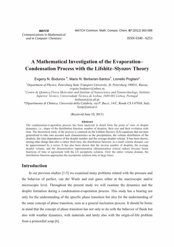
A Mathematical Investigation of the Evaporation–Condensation Process with the Lifshitz–Slyozov Theory

Evgeny N. Bodunov +, Mario N. Berberan-Santos^, Lionello Pogliani*

+Department of Physics, Petersburg State Transport University, St. Petersburg 190031, Russia, evgeny.bodunov@inbox.ru

^Centro de Química-Física Molecular and Institute of Nanoscience and Nanotechnology, Instituto Superior Técnico, Universidade Técnica de Lisboa, 1049-001 Lisboa, Portugal

berberan@ist.utl.pt *Dipartimento di Chimica, Università della Calabria, via P. Bucci, 14/C, Rende CS I-87036, Italy,

lionp@unical.it

(Received June 10, 2011)

Abstract The condensation-evaporation process has been analyzed in detail form the point of view of droplet dynamics, i.e., shape of the distribution function, number of droplets, their size and their evolution with time. The theoretical study of the process is centered on the Lifshitz-Slyozov (LS) equations that are here generalized to take into account such characteristics as the precipitation, the volume distribution of the droplets, the time dependences of the droplet number and the average droplet volume. It has been shown, among other things that after a rather short time, the distribution function, in a small volume domain, can be approximated by a series. It has also been shown that the inverse number of droplets, the average droplet volume, and the dimensionless supersaturation (dimensionless critical radius) become linear functions of time in agreement with the LS asymptotic solution. Over the entire volume domain, the distribution function approaches the asymptotic solution only at large times.

Introduction In our previous studies [1-5] we examined many problems related with the pressure and

the behavior of perfect, van der Waals and real gases either at the macroscopic and/or

microscopic level. Throughout the present study we will examine the dynamics and the

droplet formation during a condensation-evaporation process. This study has a bearing not

only for the understanding of the specific phase transition but also for the understanding of

the same concept of phase transition, seen as a general nucleation process. It should be borne

in mind that the concept of phase transition has not only to do with the behavior of fluids but

also with weather dynamics, with materials and lately also with the origin-of-life problem

from a primordial soup [6].

MATCH

Communications in Mathematical

and in Computer Chemistry

MATCH Commun. Math. Comput. Chem. 67 (2012) 563-588

ISSN 0340 - 6253

The spinodal♦ phase demixing of binary fluid mixtures occurs in three stages: (i) an early

stage where loose aggregates are spontaneously formed, (ii) an intermediate stage where the

equilibrium concentrations in both the majority and minority phases are reached, and (iii) a

final stage where aggregates grow by coarsening, to reduce their interfacial energy due to the

minor surface/volume ratio [7-9]. While the early stage is well understood, the intermediate

stage is still very controversial. The late stage mechanism depends both on the system

components and composition [10]. For solutions with near-symmetrical compositions, an

interconnected bicontinuous pattern is developed, while in very asymmetric systems

polydisperse droplets coexist with a very dilute solution. The coarsening in bicontinuous

pattern systems is driven by hydrodynamic effects [11, 12], while in asymmetric solutions it

occurs either by the evaporation-condensation mechanism of Lifshitz-Slyozov-Wagner

(LSW) [13-15] or by the diffusion-reaction mechanism of Binder-Sauffer (BS) [16, 17].

In the BS mechanism droplets travel by Brownian motion through the majority phase and

coagulate when they meet. Contrarily, in the LSW mechanism, the translation motion of the

droplets is negligible and larger droplets grow at the expense of the nearby smaller ones:

individual molecules leave small droplets, migrate through the majority phase by diffusion,

and condensate into larger droplets. This results from the decrease of the chemical potential

with droplet size increase, a phenomenon due to the surface tension. None of the BS and

LSW mechanisms consider the particle-particle interactions and are restricted to systems with

low volume fraction of the minority phase [18-20]. The BS mechanism dominates when

encounters between droplets are frequent. This depends on both the number density of

droplets and the viscosity of the medium. For this reason the coarsening in dilute viscous

systems (metal alloys and polymer blends) occurs with the LSW mechanism, while in dilute

solutions the BS mechanism takes over. Both mechanisms predict a linear increase of the

average volume of droplets with time, and its slope depends on the volume fraction of the

minority phase in the BS but not in the LSW mechanism [20]. The coarsening is responsible

for the increase in droplets volume, reducing their number without changing the majority

phase composition.

The equations describing the coarsening with the BS and LSW mechanisms have obtained

autonomous mathematical importance [21-23]. As many authors [13, 15] believed that only

one asymptotic solution to the LS equations (independent on initial volume distribution

function of droplets) exists, mathematical investigation of the generalized LS equations for

the search of new possible solutions were started [22, 23]. In this paper, we show that LS

-564-

asymptotic solution is not unique and there are other solutions that depend on the initial

conditions. Our conclusions are based not on mathematical methods (theorems and lemmas),

but on the understanding of the physics of evaporation-condensation process that is described

by the LS equations.

When droplets larger than a critical volume are formed, precipitation occurs [24-25].

Notice that precipitation is important in vapors and liquids and is absent in solid solutions

(metal alloys) where grains of new phase grow.

Precipitation and its effect on volume distribution function of droplets within the

framework of the BS theory were investigated [26] in connection with the late stage phase

demixing of a very dilute toluene solution of a poly(ethylene oxide) chain labeled at one end

with pyrene. In this work, we concentrate our attention on the evaporation-condensation

LSW mechanism. Here the Lifshitz-Slyozov (LS) equations [13, 15] are generalized to take

into account precipitation, volume distribution function of droplets, time dependences of

droplet number and average droplet volume are investigated. Considerations done in this

paper have also some bearing on the problem of quantum dots [27].

Basic Equations Let the equilibrium concentration CR at the boundary of a droplet be related to the droplet

radius R by the well known Gibbs-Thomson equation [13, 15],

R

CCR�

�� � (1)

C∞ is the concentration of the saturated solution, C∞ = CR=∞, α = 2σC∞V0/kT [m-2], σ is the

inter-phase surface tension [Nm-1], and V0 is atomic volume of the solute. Thus, the

equilibrium concentration of solute near small droplets is larger than the equilibrium

concentration near large droplets.

If we ignore the interaction between droplets (droplet sizes R are small compared with the

mean distance between them), the diffusion current of solute across the droplet boundary is

given by the following Fick’s first law, J [m-2s-1], where D0 is the diffusion coefficient [m2s-

1], and C is the population density, i.e., number of particles per volume [m-3]),

Rr

R rCDJ

���

�� 0 (2)

The change of volume of the droplet is determined by the flow of solute atoms,

-565-

Rr

R rCDVRJVRR

dtd

���

����

��

002

023 44

34 ��� (3)

Introduction of the effective diffusion coefficient, D = V0D0 [m5s-1], allows to obtain the

change of the droplet radius with time,

Rrr

CDdtdR

���

� (4)

To obtain ∂C/∂r the diffusion equation (5, where, � 2 = ∂2/∂x2 + ∂2/∂y2 + ∂2/∂z2) must be

solved with the boundary conditions (6),

CDdtdC 2

0�� (5)

RRrCC �

�, CC

r�

�� (6)

Here, )(tCC � is the average concentration in solution. At small droplet growing speed, or

under the condition of small initial supersaturation, 0C - C∞ = Δ0 << 1, )0(0 �� tCC , it is

enough to solve the stationary diffusion equation, dC/dt = 0, to obtain the flow JR, and the

result is,

� �

rCCRCC ���

�� � , �

�� ���

��

� RRrC

Rr

�1 (7)

Here, ������ CCt)( is the supersaturation at a given time. Finally, for the speed of a

growing droplet we have,

�

�� ���

RRD

dtdR � (8)

Equation (8) is valid if the characteristic time scale of the supersaturation change is much

larger than the time of establishing stationary current JR at the droplet surface. This means

-566-

that Eq (1) supposes the existence of local thermodynamic equilibrium near the droplet

surface.

Eq. (8) implies that a critical radius Rc (Rc = α/Δ) exists. If the radius of a droplet

becomes R = Rc than the droplet is in equilibrium with the solution. If R > Rc, the droplet is

growing, and if R < Rc, the droplet is vanishing, while at the initial time, the critical radius is

given by, Rc(t = 0) = Rc0 = α/Δ0.

Let us work from now on with dimensionless variables, i.e., dimensionless radius ρ = R/Rc,

dimensionless volume v = ρ3, dimensionless time t΄ = tαD/Rc03, and dimensionless

supersaturation (dimensionless critical radius) x(t) = Δ0/Δ(t) = Rc(t)/Rc0. In this way Eq (8)

can be rewritten as

��

���

�� 1

)()(3

3/1

txtv

dtdv (9)

From now on we will omit the prime on t, i.e., this omission will be maintained throughout

the remaining paper. Let function f(v,t) be the volume distribution function so that the

number of droplets in the unit volume, n(t), is given by,

��

�0

),()( dvtvftn (10)

This function f obeys the following equation of continuity,

0��

��

��

���

dtdvf

vtf (11)

By the law of matter conservation we have,

)()(000 tqtQq ������ (12)

Where Q0 is the total initial supersaturation taking into account that at time t = 0, some

amount of solute, q0, was present in the droplets (q0 has a meaning of a number of solute

-567-

atoms initially in the droplets per unit volume); q(t) is the number of solute atoms in the

droplets per unit volume given by,

� ���

�0

30

0

,3

41)( dvtvvfRV

tq c

� (13)

Taking into account that x(t) = Δ0/Δ(t) = Rc(t)/Rc0, then Eq (12) can be rewritten as,

��

��

�00

0 ),()(

11 dvtvvfktxQ

(14)

Here, 10

10

303

4 ��� QVRk c� . Equations (9), (11), and (14) together with the corresponding initial

condition [t = 0, f(v, 0)] allow to obtain the distribution function f.

Lifshitz-Slyozov Asymptotic Solution

Lifshitz and Slezov [13, 15] obtained an asymptotic solution for Eqs (9), (11), and (14),

which is independent on the initial conditions [i.e., on the shape of the distribution function at

time t = 0, f(v, 0)],

�

�� �

tvp

ttntvf

49

49)(),( (15)

Function p(z), which is here estimated at z = 9v/(4t), obeys the normalization condition,

1)(0

���

dzzp , and has the analytic form, shown in Fig. 1,

� � � �

���

���

�

�

��

��

��

���

,827,0

,827,

2/32/3exp

2/331

23

)(3/13/113/13/73/13/5

3

z

zzzz

e

zp (16)

-568-

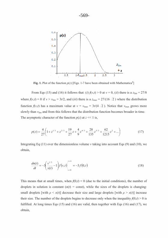
Fig. 1. Plot of the function p(z) [Figs. 1-7 have been obtained with Mathematica♯]

From Eqs (15) and (16) it follows that: (i) f(v,t) > 0 at v = 0, (ii) there is a zlim = 27/8

where f(v,t) = 0 if v > vlim = 3t/2, and (iii) there is a zmax = 27/(16 2 ) where the distribution

function f(v,t) has a maximum value at v = vmax = 3t/(4 2 ). Notice that vmax grows more

slowly than vlim and from this follows that the distribution function becomes broader in time.

The asymptotic character of the function p(z) at z << 1 is,

�

�� �������� ...

121562

13528

94

27191

274)( 23/53/43/23/1 zzzzzzzp (17)

Integrating Eq (11) over the dimensionless volume v taking into account Eqs (9) and (10), we

obtain,

� � � �tftvftx

vdt

tdnv

v

,03,1)(

3)(

0

3/1

����

���

���

��

�

(18)

This means that at small times, when f(0,t) = 0 (due to the initial conditions), the number of

droplets in solution is constant (n(t) = const), while the sizes of the droplets is changing:

small droplets [with ρ < x(t)] decrease their size and large droplets [with ρ > x(t)] increase

their size. The number of the droplets begins to decrease only when the inequality f(0,t) > 0 is

fulfilled. At long times Eqs (15) and (16) are valid, then together with Eqs (16) and (17), we

obtain,

-569-

)(1274)(

493)( tn

ttn

tdttdn

���� (19)

The solution to this equation is,

ttn

tn 00)( � (20)

Here, n0 is the number of droplets in the unit volume at time t0. Cited authors [13, 15] have

also obtained,

ttx94)(3 � (21)

Now, using Eqs (15) and (16), it is possible to obtain, 13/1 �z and 1296.1�z . Thus, the

average droplet radius and the average droplet volume, � and v , are,

3/1394)( ttx ��� , tv 502.03 �� � (22)

Authors [13, 15] believe that the obtained results are independent on the initial conditions

if the initial distribution function has a finite width and is continuous (not a sum of δ-

function). Other authors [22, 23] questioned this statement and found some new solutions

that contradict it. We begin our investigation of the basic equations with the distribution

function that equals a sum of δ-function, because it will help us to understand the behavior of

the distribution function from a physical point of view.

Note that the modified distribution function (15) and (16) is often used as distribution

function of quantum dots [27-29]. Let us introduce the relative radius of the droplets

(quantum dots) u = �� / and take into account, according to the definition of z and Eq (22),

the droplet volume v = ρ3, dv = 3ρ2dρ, and z1/3 = u. If � is the average radius of the droplets

-570-

(quantum dots), the normalized distribution function of the droplets (quantum dots) over their

radius, N(u), ��

�0

,1)( �duN can be obtained from Eqs (15) and (16) [28, 29],

4 22

5/3 7/3 11/3

( , ) 3 1 3 / 2( ) 3 exp , 3 / 2,( ) 2 ( 3) (3 / 2 ) 3 / 2

( ) 0, 3 / 2.

f v t e uN u u un t u u u

N u u

� � � � �� �� � ��

� �

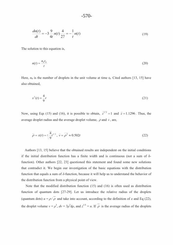
Solution of the basic equations with monodisperse distribution of droplets In the case of initial monodisperse distribution of droplets, this distribution, according to the basic equations and to the physics of the process, continues to be monodisperse at any time. Let at time t = 0 be f(v,0) = n0δ(v-v0), i.e., the initial droplet volume is v(t = 0) = v0. For longer times according to the basic equations and the physics of the process under investigation, f(v, t) continues to be a δ-function and the number of droplets is constant, i.e., f(v, t) = n0δ(v-v(t)) where v(t) senses the droplet volume, v(t) = ρ3(t), and obeys Eq. (9). At this condition, the basic Eq. (14) becomes

)()(

1 tbvtx

a�� (23)

Where, a = Δ0/Q0, and b = n0k. Note, that if the initial size v0 of the droplet is larger than the critical size, the droplets grows, v1/3(t) > x(t), until the establishment of equilibrium conditions, when the droplet stops growing. Thus, the physical process foretells that at some t → ∞, dv/dt = 0 and from Eq. (9) we obtain, v(∞) = x3(∞) (Fig. 2).

Fig. 2. The v(t) (higher curve) and x(t)3 (lower curve) functions at: b = 0.01, and v0 = 5

-571-

At time t = 0, x(0) = 1, v(0) = v0, and from Eq. (23) we have that, 1 = a + bv0, i.e., a = 1 – bv0.

From Eq. (23), we get, 01)(1)(1

)(1

bvtbv

atbv

tx ��

��

� . Inserting this equation into Eq (9), we

obtain,

��

���

�

��

� 1113

0

3/1

bvbvv

dtdv (24)

Equation (24) can be solved with Mathematica♯. For growing droplets (v0 > 1), the

concentration of the solution and Δ(t) decrease, therefore x(t) = Δ0/Δ(t) increase. At t → ∞,

the process of droplet growing stops, dv/dt = 0, and in accordance with Eq. (9), v(∞) = x3(∞)

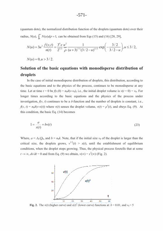
(see Fig. 2). For dissolving droplets (v0 < 1), instead, the concentration of the solution and

Δ(t) increase, therefore x(t) = Δ0/Δ(t) decreases. At some later moment t, all droplets dissolve,

v(t) = 0, and from Eq. (23), we obtain x(t) = a = 1 – bv0. Fig. 3 illustrates this behavior.

Fig. 3. The v(t) (lower curve)and x(t)3 (upper curve) functions at: b = 0.1, and v0 = 0.9

The distribution function of the droplets is the sum of two δ-functions According to the basic LS equation (9, 11, and 14) for this case, if the initial distribution function is a sum of two δ-functions it continues to be a sum of two δ-functions with the same coefficients (the numbers of droplets of two different volumes are constant) at later times. Let f(v, t) = n0{δ(v-v1(t)) + δ(v-v2(t))}. For simplicity, we suppose that the numbers of the droplets of different size are equal to n0. Their initial volumes are v1(0) = v10 and v2(0) = v20. With this condition, the basic equations (9) and (14) become,

-572-

��

���

�� 1

)()(

33/1

11

txtv

dtdv (25)

��

���

�� 1

)()(3

3/122

txtv

dtdv (26)

))()(()(

1 21 tvtvbtx

a��� (27)

Parameters a and b have the same meaning as before. At time t = 0, x(0) = 1, v1(0) = v10, and v2(0) = v20, and from Eq. (27) we have 1 = a + b(v10 + v20). Thus a = 1 – b(v10 + v20) and from

Eq (23) we get, )(1))()((1))()((1

)(1

2010

2121

vvbtvtvb

atvtvb

tx ����

���

� . Inserting this equation into

Eq (25) and (26), we obtain,

��

���

�

����

� 1)(1

)(13

2010

213/11

1

vvbvvbv

dtdv

(28)

��

���

�

����

� 1)(1

)(132010

213/12

2

vvbvvbv

dtdv

(29)

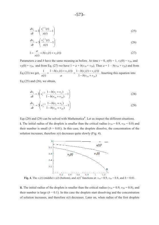
Eqs (28) and (29) can be solved with Mathematica♯. Let us inspect the different situations. i. The initial radius of the droplets is smaller than the critical radius (v10 = 0.9, v20 = 0.8) and their number is small (b = 0.01). In this case, the droplets dissolve, the concentration of the solution increases, therefore x(t) decreases quite slowly (Fig. 4).

Fig. 4. The v1(t) (middle) v2(t) (bottom), and x(t)3 functions at: v10 = 0.9, v20 = 0.8, and b = 0.01. ii. The initial radius of the droplets is smaller than the critical radius (v10 = 0.9, v20 = 0.8), and their number is large (b = 0.1). In this case the droplets start dissolving and the concentration of solution increases, and therefore x(t) decreases. Later on, when radius of the first droplets

-573-

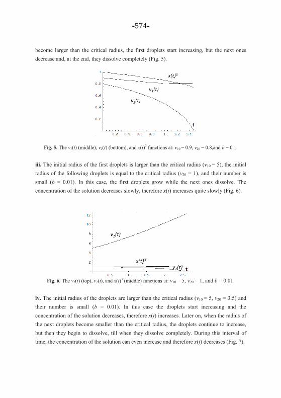
become larger than the critical radius, the first droplets start increasing, but the next ones decrease and, at the end, they dissolve completely (Fig. 5).

Fig. 5. The v1(t) (middle), v2(t) (bottom), and x(t)3 functions at: v10 = 0.9, v20 = 0.8,and b = 0.1.

iii. The initial radius of the first droplets is larger than the critical radius (v10 = 5), the initial radius of the following droplets is equal to the critical radius (v20 = 1), and their number is small (b = 0.01). In this case, the first droplets grow while the next ones dissolve. The concentration of the solution decreases slowly, therefore x(t) increases quite slowly (Fig. 6).

Fig. 6. The v1(t) (top), v2(t), and x(t)3 (middle) functions at: v10 = 5, v20 = 1, and b = 0.01.

iv. The initial radius of the droplets are larger than the critical radius (v10 = 5, v20 = 3.5) and their number is small (b = 0.01). In this case the droplets start increasing and the concentration of the solution decreases, therefore x(t) increases. Later on, when the radius of the next droplets become smaller than the critical radius, the droplets continue to increase, but then they begin to dissolve, till when they dissolve completely. During this interval of time, the concentration of the solution can even increase and therefore x(t) decreases (Fig. 7).

-574-

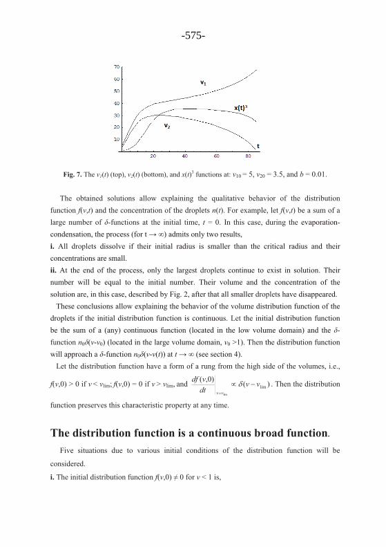
Fig. 7. The v1(t) (top), v2(t) (bottom), and x(t)3 functions at: v10 = 5, v20 = 3.5, and b = 0.01.

The obtained solutions allow explaining the qualitative behavior of the distribution function f(v,t) and the concentration of the droplets n(t). For example, let f(v,t) be a sum of a large number of δ-functions at the initial time, t = 0. In this case, during the evaporation-condensation, the process (for t → ∞) admits only two results, i. All droplets dissolve if their initial radius is smaller than the critical radius and their concentrations are small. ii. At the end of the process, only the largest droplets continue to exist in solution. Their number will be equal to the initial number. Their volume and the concentration of the solution are, in this case, described by Fig. 2, after that all smaller droplets have disappeared. These conclusions allow explaining the behavior of the volume distribution function of the droplets if the initial distribution function is continuous. Let the initial distribution function be the sum of a (any) continuous function (located in the low volume domain) and the δ-function n0δ(v-v0) (located in the large volume domain, v0 >1). Then the distribution function will approach a δ-function n0δ(v-v(t)) at t → ∞ (see section 4). Let the distribution function have a form of a rung from the high side of the volumes, i.e.,

f(v,0) > 0 if v < vlim; f(v,0) = 0 if v > vlim, and )()0,(lim

lim

vvdtvdf

vv

���

� . Then the distribution

function preserves this characteristic property at any time.

The distribution function is a continuous broad function.

Five situations due to various initial conditions of the distribution function will be

considered.

i. The initial distribution function f(v,0) ≠ 0 for v < 1 is,

-575-

� �� ���

��

�

�����

�

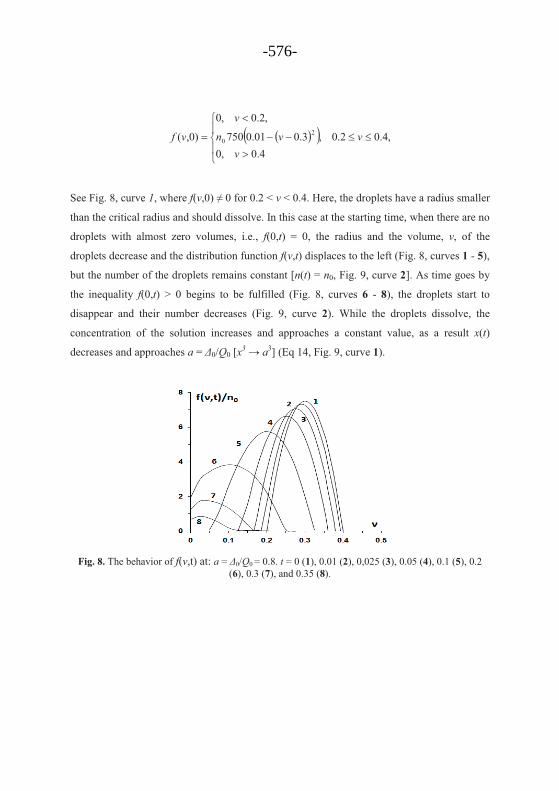
�4.0,0

,4.02.0,3.001.0750

,2.0,0

)0,( 20

vvvn

v

vf

See Fig. 8, curve 1, where f(v,0) ≠ 0 for 0.2 < v < 0.4. Here, the droplets have a radius smaller

than the critical radius and should dissolve. In this case at the starting time, when there are no

droplets with almost zero volumes, i.e., f(0,t) = 0, the radius and the volume, v, of the

droplets decrease and the distribution function f(v,t) displaces to the left (Fig. 8, curves 1 - 5),

but the number of the droplets remains constant [n(t) = n0, Fig. 9, curve 2]. As time goes by

the inequality f(0,t) > 0 begins to be fulfilled (Fig. 8, curves 6 - 8), the droplets start to

disappear and their number decreases (Fig. 9, curve 2). While the droplets dissolve, the

concentration of the solution increases and approaches a constant value, as a result x(t)

decreases and approaches a = Δ0/Q0 [x3 → a3] (Eq 14, Fig. 9, curve 1).

Fig. 8. The behavior of f(v,t) at: a = Δ0/Q0 = 0.8. t = 0 (1), 0.01 (2), 0,025 (3), 0.05 (4), 0.1 (5), 0.2 (6), 0.3 (7), and 0.35 (8).

6

-576-

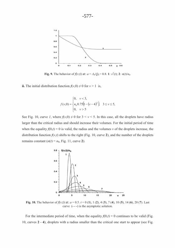
Fig. 9. The behavior of f(v,t) at: a = Δ0/Q0 = 0.8. 1: x3(t); 2: n(t)/n0.

ii. The initial distribution function f(v,0) ≠ 0 for v > 1 is,

� �� ���

��

�

�����

�

�5,0

,53,4175.0

,3,0

)0,( 20

vvvn

v

vf

See Fig. 10, curve 1, where f(v,0) ≠ 0 for 3 < v < 5. In this case, all the droplets have radius

larger than the critical radius and should increase their volumes. For the initial period of time

when the equality f(0,t) = 0 is valid, the radius and the volumes v of the droplets increase, the

distribution function f(v,t) shifts to the right (Fig. 10, curve 2), and the number of the droplets

remains constant (n(t) = n0, Fig. 11, curve 2).

Fig. 10. The behavior of f(v,t) at: a = 0.5. t = 0 (1), 1 (2), 4 (3), 7 (4), 10 (5), 14 (6), 20 (7). Last curve (- - -) is the asymptotic solution.

For the intermediate period of time, when the equality f(0,t) = 0 continues to be valid (Fig.

10, curves 2 - 4), droplets with a radius smaller than the critical one start to appear (see Fig.

-577-

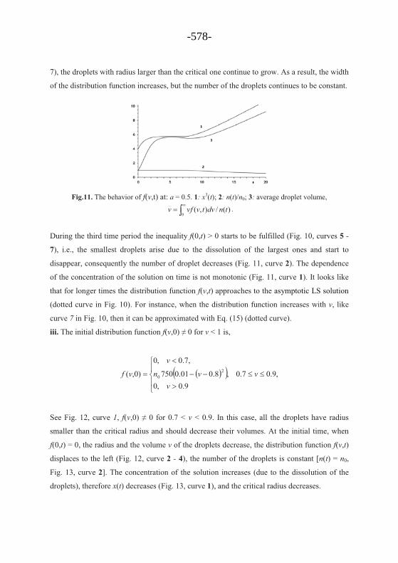
7), the droplets with radius larger than the critical one continue to grow. As a result, the width

of the distribution function increases, but the number of the droplets continues to be constant.

Fig.11. The behavior of f(v,t) at: a = 0.5. 1: x3(t); 2: n(t)/n0; 3: average droplet volume,

)(/),(0

tndvtvvfv ��

� .

During the third time period the inequality f(0,t) > 0 starts to be fulfilled (Fig. 10, curves 5 -

7), i.e., the smallest droplets arise due to the dissolution of the largest ones and start to

disappear, consequently the number of droplet decreases (Fig. 11, curve 2). The dependence

of the concentration of the solution on time is not monotonic (Fig. 11, curve 1). It looks like

that for longer times the distribution function f(v,t) approaches to the asymptotic LS solution

(dotted curve in Fig. 10). For instance, when the distribution function increases with v, like

curve 7 in Fig. 10, then it can be approximated with Eq. (15) (dotted curve).

iii. The initial distribution function f(v,0) ≠ 0 for v < 1 is,

� �� ���

��

�

�����

�

�9.0,0

,9.07.0,8.001.0750

,7.0,0

)0,( 20

vvvn

v

vf

See Fig. 12, curve 1, f(v,0) ≠ 0 for 0.7 < v < 0.9. In this case, all the droplets have radius

smaller than the critical radius and should decrease their volumes. At the initial time, when

f(0,t) = 0, the radius and the volume v of the droplets decrease, the distribution function f(v,t)

displaces to the left (Fig. 12, curve 2 - 4), the number of the droplets is constant [n(t) = n0,

Fig. 13, curve 2]. The concentration of the solution increases (due to the dissolution of the

droplets), therefore x(t) decreases (Fig. 13, curve 1), and the critical radius decreases.

-578-

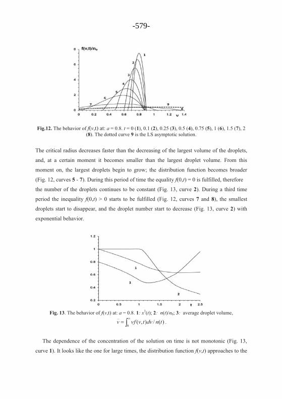
Fig.12. The behavior of f(v,t) at: a = 0.8. t = 0 (1), 0.1 (2), 0.25 (3), 0.5 (4), 0.75 (5), 1 (6), 1.5 (7), 2 (8). The dotted curve 9 is the LS asymptotic solution.

The critical radius decreases faster than the decreasing of the largest volume of the droplets,

and, at a certain moment it becomes smaller than the largest droplet volume. From this

moment on, the largest droplets begin to grow; the distribution function becomes broader

(Fig. 12, curves 5 - 7). During this period of time the equality f(0,t) = 0 is fulfilled, therefore

the number of the droplets continues to be constant (Fig. 13, curve 2). During a third time

period the inequality f(0,t) > 0 starts to be fulfilled (Fig. 12, curves 7 and 8), the smallest

droplets start to disappear, and the droplet number start to decrease (Fig. 13, curve 2) with

exponential behavior.

Fig. 13. The behavior of f(v,t) at: a = 0.8. 1: x3(t); 2: n(t)/n0; 3: average droplet volume,

)(/),(0

tndvtvvfv ��

� .

The dependence of the concentration of the solution on time is not monotonic (Fig. 13,

curve 1). It looks like the one for large times, the distribution function f(v,t) approaches to the

-579-

LS asymptotic solution (curve 9 in Fig. 12), i.e., curve 8 (within the domain, where the

distribution function grows with v) can be approximated by Eq (15) (dotted curve 9).

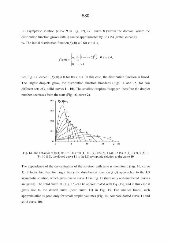
iv. The initial distribution function f(v,0) ≠ 0 for v < 4 is,

� �� ���

���

�

�����

4,0

,40,24323

)0,(2

0

v

vvnvf

See Fig. 14, curve 1, f(v,0) ≠ 0 for 0< v < 4. In this case, the distribution function is broad.

The largest droplets grow, the distribution function broadens (Figs 14 and 15, for two

different sets of t, solid curves 1 - 10). The smallest droplets disappear, therefore the droplet

number decreases from the start (Fig. 16, curve 2).

Fig. 14. The behavior of f(v,t) at: a = 0.8. t = 0 (1), 0.1 (2), 0.5 (3), 1 (4), 1.5 (5), 2 (6), 3 (7), 5 (8), 7 (9), 10 (10), the dotted curve 11 is the LS asymptotic solution to the curve 10.

The dependence of the concentration of the solution with time is monotonic (Fig. 16, curve

1). It looks like that for larger times the distribution function f(v,t) approaches to the LS

asymptotic solution, which gives rise to curve 11 in Fig. 15 (here only odd-numbered curves

are given). The solid curve 11 (Fig. 15) can be approximated with Eq. (15), and in this case it

gives rise to the dotted curve (near curve 11) in Fig. 15. For smaller times, such

approximation is good only for small droplet volumes (Fig. 14, compare dotted curve 11 and

solid curve 10).

-580-

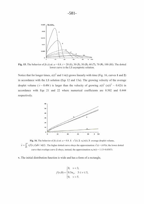
Fig. 15. The behavior of f(v,t) at: a = 0.8. t = 20 (1), 30 (3), 50 (5), 60 (7), 70 (9), 100 (11). The dotted

lower curve is the LS asymptotic solution.

Notice that for longer times, x(t)3 and 1/n(t) grows linearly with time (Fig. 16, curves 1 and 2)

in accordance with the LS solution (Eqs 12 and 13a). The growing velocity of the average

droplet volume ( tv 49.0~ ) is larger than the velocity of growing x(t)3 (x(t)3 ~ 0.42t) in

accordance with Eqs 21 and 22 where numerical coefficients are 0.502 and 0.444

respectively.

Fig. 16. The behavior of f(v,t) at: a = 0.8. 1: x3(t); 2: n0/n(t); 3: average droplet volume,

)(/),(0

tndvtvvfv ��

� . The higher dotted curve obeys the approximation x3(t) = (4/9)t; the lower dotted

curve that overlaps curve 2 obeys, instead, the approximation n0/n(t) = 1.13+0.0587t.

v. The initial distribution function is wide and has a form of a rectangle,

��

��

�

���

��

.5,0,53,5.0

,3,0)0,( 0

vvn

vvf

-581-

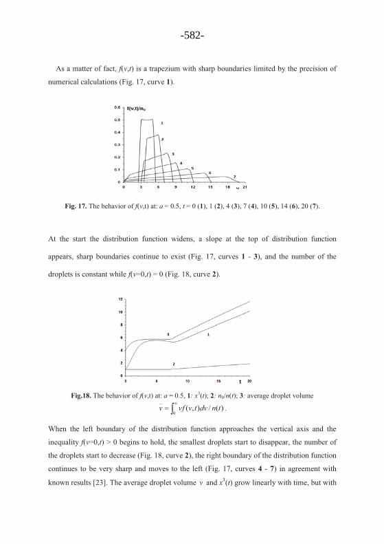
As a matter of fact, f(v,t) is a trapezium with sharp boundaries limited by the precision of

numerical calculations (Fig. 17, curve 1).

Fig. 17. The behavior of f(v,t) at: a = 0.5, t = 0 (1), 1 (2), 4 (3), 7 (4), 10 (5), 14 (6), 20 (7).

At the start the distribution function widens, a slope at the top of distribution function

appears, sharp boundaries continue to exist (Fig. 17, curves 1 - 3), and the number of the

droplets is constant while f(v=0,t) = 0 (Fig. 18, curve 2).

Fig.18. The behavior of f(v,t) at: a = 0.5, 1: x3(t); 2: n0/n(t); 3: average droplet volume

)(/),(0

tndvtvvfv ��

� .

When the left boundary of the distribution function approaches the vertical axis and the

inequality f(v=0,t) > 0 begins to hold, the smallest droplets start to disappear, the number of

the droplets start to decrease (Fig. 18, curve 2), the right boundary of the distribution function

continues to be very sharp and moves to the left (Fig. 17, curves 4 - 7) in agreement with

known results [23]. The average droplet volume v and x3(t) grow linearly with time, but with

-582-

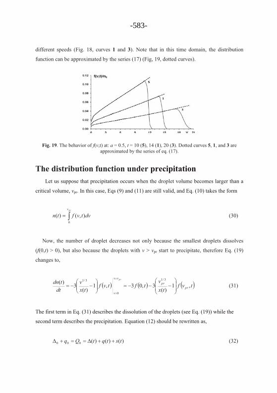
different speeds (Fig. 18, curves 1 and 3). Note that in this time domain, the distribution

function can be approximated by the series (17) (Fig, 19, dotted curves).

Fig. 19. The behavior of f(v,t) at: a = 0.5, t = 10 (5), 14 (1), 20 (3). Dotted curves 5, 1, and 3 are approximated by the series of eq. (17).

The distribution function under precipitation Let us suppose that precipitation occurs when the droplet volume becomes larger than a

critical volume, vpr. In this case, Eqs (9) and (11) are still valid, and Eq. (10) takes the form

��prv

dvtvftn0

),()( (30)

Now, the number of droplet decreases not only because the smallest droplets dissolves

(f(0,t) > 0), but also because the droplets with v > vpr start to precipitate, therefore Eq. (19)

changes to,

� � � � � �tvftx

vtftvf

txv

dttdn

prpr

vv

v

pr

,1)(

3,03,1)(

3)( 3/1

0

3/1

��

���

������

���

���

�

�

(31)

The first term in Eq. (31) describes the dissolution of the droplets (see Eq. (19)) while the

second term describes the precipitation. Equation (12) should be rewritten as,

)()()(000 tstqtQq ������� (32)

-583-

s(t) is the number of solute atoms per unit volume that precipitated in the droplets. Here, [see

Eq. (13)]

� ���prv

c dvtvvfRV

tq0

30

0

,3

41)( � (33)

From Eq. (31), it follows that, 30

0

3/1

3411

)(),(3 c

prpr R

Vtxv

tvfdtds �

��

���

�� Supposing that there

were no droplets with volumes larger than vpr at the initial time t = 0, we obtain,

'

0'

3/1'3

00

1)(

),(33

41)( dttx

vtvfR

Vts

tpr

prc � ��

���

��

� (34)

Finally, Eq. (14) takes the form

)(1),()(

11000

0 tsQ

dvtvvfktxQ

prv

���

� � (35)

Here, 10

10

303

4 ��� QVRk c� . To obtain the needed dependences, Eqs (9), (11), (30), (34), and

(35) must be solved. In the calculations below, we suppose that vpr = 10 and the initial

distribution function f(v,0) ≠ 0 for v < 4 (as in the case iv) is,

� �� ���

���

�

�����

4,0

,40,24323

)0,(2

0

v

vvnvf

This distribution function is shown in Fig. 20, curve 1. Solutions of equations (9), (11), (30),

(34), and (35) for t > 0 are also shown in Fig. 20. For small times, while there are no droplets

with volumes larger than vpr , f(vpr,t) = 0, curves 1 - 7 (in Fig. 20) repeat curves 1 - 7 in Fig.

14. In this time domain, the behavior of parameters x3(t), n0/n(t) and v (Fig. 21) are the same

as in Fig. 16.

-584-

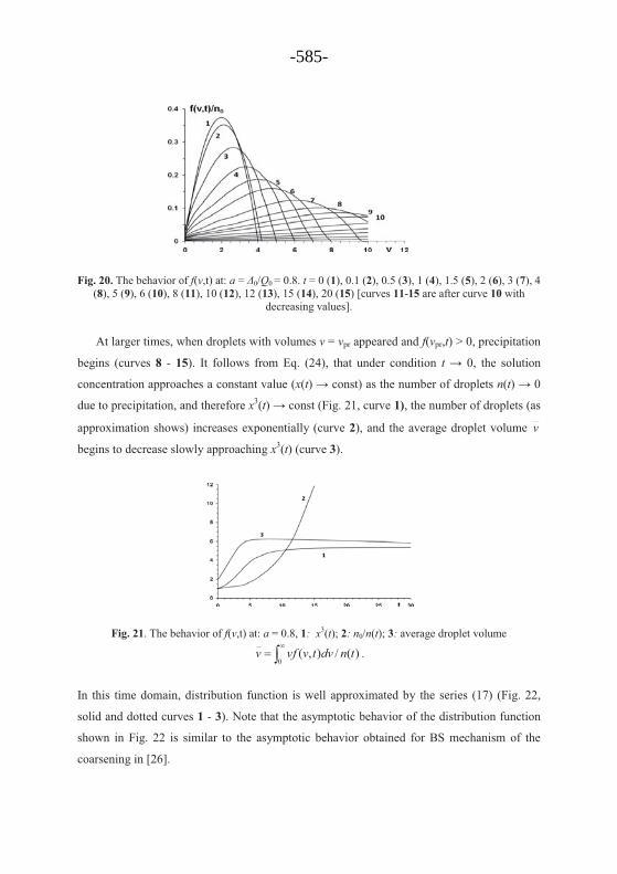
Fig. 20. The behavior of f(v,t) at: a = Δ0/Q0 = 0.8. t = 0 (1), 0.1 (2), 0.5 (3), 1 (4), 1.5 (5), 2 (6), 3 (7), 4 (8), 5 (9), 6 (10), 8 (11), 10 (12), 12 (13), 15 (14), 20 (15) [curves 11-15 are after curve 10 with

decreasing values].

At larger times, when droplets with volumes v = vpr appeared and f(vpr,t) > 0, precipitation

begins (curves 8 - 15). It follows from Eq. (24), that under condition t → 0, the solution

concentration approaches a constant value (x(t) → const) as the number of droplets n(t) → 0

due to precipitation, and therefore x3(t) → const (Fig. 21, curve 1), the number of droplets (as

approximation shows) increases exponentially (curve 2), and the average droplet volume v

begins to decrease slowly approaching x3(t) (curve 3).

Fig. 21. The behavior of f(v,t) at: a = 0.8, 1: x3(t); 2: n0/n(t); 3: average droplet volume

)(/),(0

tndvtvvfv ��

� .

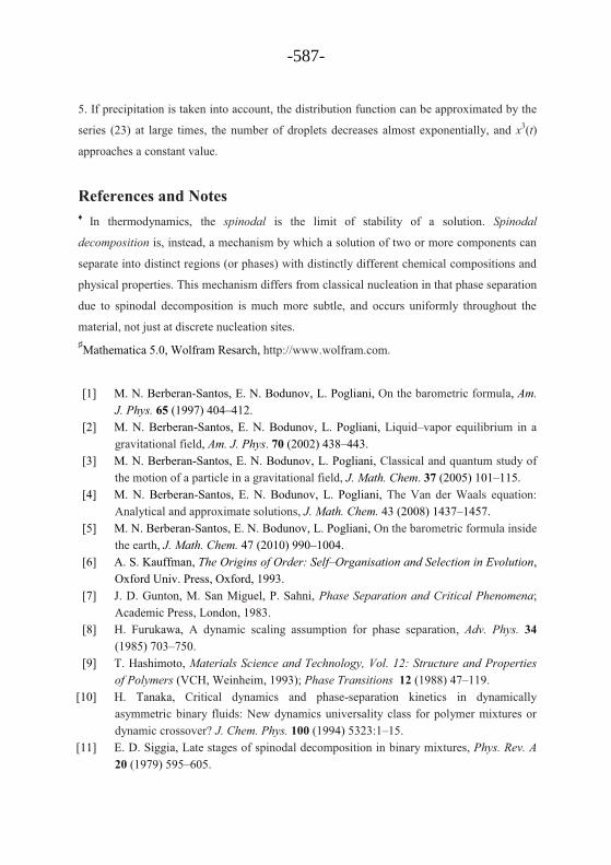
In this time domain, distribution function is well approximated by the series (17) (Fig. 22,

solid and dotted curves 1 - 3). Note that the asymptotic behavior of the distribution function

shown in Fig. 22 is similar to the asymptotic behavior obtained for BS mechanism of the

coarsening in [26].

-585-

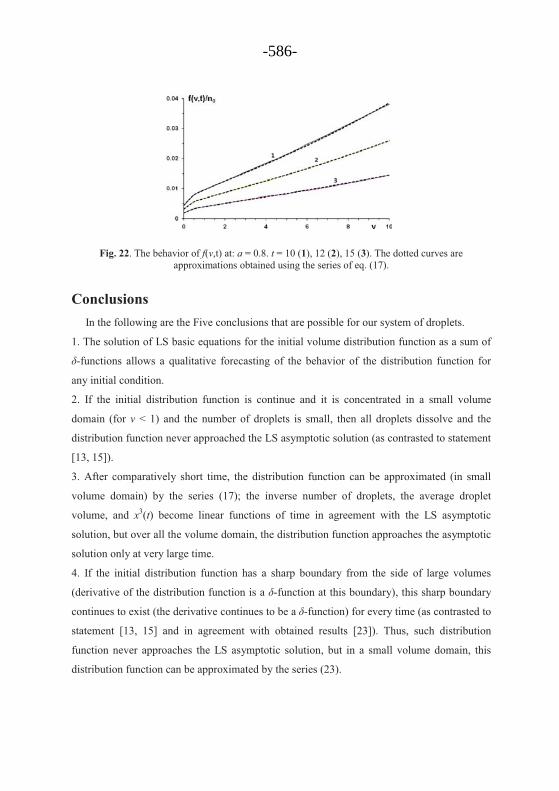
Fig. 22. The behavior of f(v,t) at: a = 0.8. t = 10 (1), 12 (2), 15 (3). The dotted curves are approximations obtained using the series of eq. (17).

Conclusions In the following are the Five conclusions that are possible for our system of droplets.

1. The solution of LS basic equations for the initial volume distribution function as a sum of

δ-functions allows a qualitative forecasting of the behavior of the distribution function for

any initial condition.

2. If the initial distribution function is continue and it is concentrated in a small volume

domain (for v < 1) and the number of droplets is small, then all droplets dissolve and the

distribution function never approached the LS asymptotic solution (as contrasted to statement

[13, 15]).

3. After comparatively short time, the distribution function can be approximated (in small

volume domain) by the series (17); the inverse number of droplets, the average droplet

volume, and x3(t) become linear functions of time in agreement with the LS asymptotic

solution, but over all the volume domain, the distribution function approaches the asymptotic

solution only at very large time.

4. If the initial distribution function has a sharp boundary from the side of large volumes

(derivative of the distribution function is a δ-function at this boundary), this sharp boundary

continues to exist (the derivative continues to be a δ-function) for every time (as contrasted to

statement [13, 15] and in agreement with obtained results [23]). Thus, such distribution

function never approaches the LS asymptotic solution, but in a small volume domain, this

distribution function can be approximated by the series (23).

-586-

5. If precipitation is taken into account, the distribution function can be approximated by the

series (23) at large times, the number of droplets decreases almost exponentially, and x3(t)

approaches a constant value.

References and Notes ♦ In thermodynamics, the spinodal is the limit of stability of a solution. Spinodal

decomposition is, instead, a mechanism by which a solution of two or more components can

separate into distinct regions (or phases) with distinctly different chemical compositions and

physical properties. This mechanism differs from classical nucleation in that phase separation

due to spinodal decomposition is much more subtle, and occurs uniformly throughout the

material, not just at discrete nucleation sites. ♯Mathematica 5.0, Wolfram Resarch, http://www.wolfram.com.

[1] M. N. Berberan-Santos, E. N. Bodunov, L. Pogliani, On the barometric formula, Am. J. Phys. 65 (1997) 404–412.

[2] M. N. Berberan-Santos, E. N. Bodunov, L. Pogliani, Liquid–vapor equilibrium in a gravitational field, Am. J. Phys. 70 (2002) 438–443.

[3] M. N. Berberan-Santos, E. N. Bodunov, L. Pogliani, Classical and quantum study of the motion of a particle in a gravitational field, J. Math. Chem. 37 (2005) 101–115.

[4] M. N. Berberan-Santos, E. N. Bodunov, L. Pogliani, The Van der Waals equation: Analytical and approximate solutions, J. Math. Chem. 43 (2008) 1437–1457.

[5] M. N. Berberan-Santos, E. N. Bodunov, L. Pogliani, On the barometric formula inside the earth, J. Math. Chem. 47 (2010) 990–1004.

[6] A. S. Kauffman, The Origins of Order: Self–Organisation and Selection in Evolution, Oxford Univ. Press, Oxford, 1993.

[7] J. D. Gunton, M. San Miguel, P. Sahni, Phase Separation and Critical Phenomena; Academic Press, London, 1983.

[8] H. Furukawa, A dynamic scaling assumption for phase separation, Adv. Phys. 34 (1985) 703–750.

[9] T. Hashimoto, Materials Science and Technology, Vol. 12: Structure and Properties of Polymers (VCH, Weinheim, 1993); Phase Transitions 12 (1988) 47–119.

[10] H. Tanaka, Critical dynamics and phase-separation kinetics in dynamically asymmetric binary fluids: New dynamics universality class for polymer mixtures or dynamic crossover? J. Chem. Phys. 100 (1994) 5323:1–15.

[11] E. D. Siggia, Late stages of spinodal decomposition in binary mixtures, Phys. Rev. A 20 (1979) 595–605.

-587-

[12] H. Tanaka, A new coarsening mechanism of droplet spinodal decomposition, Phys. Rev. E51 (1995) 1313.

[13] I. M. Lifshitz, V. V. Slyozov, The kinetics of precipitation from supersaturated solid solutions, J. Phys. Chem. Solids 19 (1961) 35–50.

[14] C. Wagner, Theorie der Alterung von Niederschlägen durch Umlösen (Ostwald–Reifung), Z. Elektrochem. 65 (1961) 581–591.

[15] V. V. Slezov, V. V. Sagalovich, Diffusive decomposition of solid solutions, Sov. Phys. Uspekhi 30 (1987) 23–45.

[16] K. Binder, D. Stauffer, Theory for the slowing down of the relaxation and spinodal decomposition of binary mixtures, Phys. Rev. Lett. 33 (1974) 1006–1009.

[17] K. Binder, D. Stauffer, Statistical theory of nucleation, condensation and coagulation, Adv. Phys. 25 (1976) 343–396.

[18] M. San Miguel, M. Grant, J. D. Gunton, Phase separation in two-dimensional binary fluids, Phys. Rev. A31 (1985) 1001–1005.

[19] H. Tanaka, New coarsening mechanisms for spinodal decomposition having droplet pattern in binary fluid mixture: Collision-induced collisions, Phys. Rev. Lett. 72 (1994) 1702–1705.

[20] H. Tanaka, A new coarsening mechanism of droplet spinodal decomposition, J. Chem. Phys. 103 (1995) 2361:1–4.

[21] J. M. Ball, J. Carr, O. Penrose, The Becker-Döring equations: Basic properties and asymptotic behavior of solutions, Commun. Math. Phys. 104 (1986) 657–692.

[22] B. Niethammer, R. L. Pego, The LSW model for domain coarsening: Asymptotic behavior for conserved total mass, J. Stat. Phys. 104 (2001) 1113–1144.

[23] J. A. Carrillo, T. Goudon, A numerical study on large-time asymptotic of the Lifshitz-Slyozov system, J. Sci. Comput. 20 (2004) 69–113.

[24] J. R. Philip, D. E. Smiles, Macroscopic analysis of the behavior of colloidal suspensions, Adv. Colloid Interface Sci. 17 (1982) 83–103.

[25] R. J. Hunter, Foundations of Colloid Science, Oxford Univ. Press, Oxford, 1987. [26] S. Picarra, E. J. N. Pereira, E. N. Bodunov, J. M. G. Martinho, Kinetics of coarsening

and precipitation of dilute polymer solutions: Fluorescence study of PEO in toluene, Macromolecules 35 (2002) 6397–6403.

[27] E. Bodunov, M. N. Berberan-Santos, L. Pogliani, On the shape of quantum-dot distribution-function on sizes, Optics Spectroscopy 111 (2011) 66–70.

[28] M. Ivanda, K. Babocsi, C. Dem, M. Schmitt, M. Montagna, W. Kiefer, Low-wave-number Raman scattering from CdSxSe1-x quantum dots embedded in a glass matrix, Phys. Rev. B67 (2003) 235329:1–8.

[29] M. Yu. Leonov, A. B. Baranov, A. B. Fedorov, Transient interband light absorption by quantum dots: Degenerate pump–probe spectroscopy, Optics Spectroscopy 109 (2010) 358–365

-588-