A Matrix Splitting Method for Composite Function Minimization

Ganzhao Yuan1,2, Wei-Shi Zheng2,3, Bernard Ghanem1

1King Abdullah University of Science and Technology (KAUST), Saudi Arabia2School of Data and Computer Science, Sun Yat-sen University (SYSU), China

3Key Laboratory of Machine Intelligence and Advanced Computing (Sun Yat-sen University), Ministry of Education, China

yuanganzhao@gmail.com, wszheng@ieee.org, bernard.ghanem@kaust.edu.sa

Abstract

Composite function minimization captures a wide spec-

trum of applications in both computer vision and ma-

chine learning. It includes bound constrained optimiza-

tion and cardinality regularized optimization as special cas-

es. This paper proposes and analyzes a new Matrix Split-

ting Method (MSM) for minimizing composite functions. It

can be viewed as a generalization of the classical Gauss-

Seidel method and the Successive Over-Relaxation method

for solving linear systems in the literature. Incorporating

a new Gaussian elimination procedure, the matrix splitting

method achieves state-of-the-art performance. For convex

problems, we establish the global convergence, convergence

rate, and iteration complexity of MSM, while for non-convex

problems, we prove its global convergence. Finally, we vali-

date the performance of our matrix splitting method on two

particular applications: nonnegative matrix factorization

and cardinality regularized sparse coding. Extensive exper-

iments show that our method outperforms existing compos-

ite function minimization techniques in term of both efficien-

cy and efficacy.

1. Introduction

In this paper, we focus on the following composite func-

tion minimization problem:

minx

f(x) , q(x) + h(x); q(x) = 12x

TAx+ xTb (1)

where x ∈ Rn, b ∈ R

n, A ∈ Rn×n is a positive semidef-

inite matrix, h(x) is a piecewise separable function (i.e.

h(x) =∑n

i=1 h(xi)) but not necessarily convex. Typical

examples of h(x) include the bound constrained function

and the ℓ0 and ℓ1 norm functions.

The optimization in (1) is flexible enough to model a

variety of applications of interest in both computer vision

and machine learning, including compressive sensing [7],

nonnegative matrix factorization [16, 18, 9], sparse coding

[17, 1, 2, 29], support vector machine [11], logistic regres-

sion [38], subspace clustering [8], to name a few. Although

we only focus on the quadratic function q(·), our method

can be extended to handle general composite functions as

well, by considering a typical Newton approximation of the

objective [35, 40].

The most popular method for solving (1) is perhaps the

proximal gradient method [25, 3]. It considers a fixed-

point proximal iterative procedure xk+1 = proxγh(xk −

γ▽q(xk)) based on the current gradient ▽q(xk). Here the

proximal operator proxh(a) = argminx12‖x−a‖22+ h(x)

can often be evaluated analytically, γ = 1/L is the step

size with L being the local (or global) Lipschitz constan-

t. It is guaranteed to decrease the objective at a rate of

O(L/k), where k is the iteration number. The accelerat-

ed proximal gradient method can further boost the rate to

O(L/k2). Tighter estimates of the local Lipschitz constant

leads to better convergence rate, but it scarifies additional

computation overhead to compute L. Our method is also a

fixed-point iterative method, but it does not rely on a sparse

eigenvalue solver or line search backtracking to compute

such a Lipschitz constant, and it can exploit the specified

structure of the quadratic Hessian matrix A.

The proposed method is essentially a generalization of

the classical Gauss-Seidel (GS) method and Successive

Over-Relaxation (SOR) method [6, 31]. In numerical lin-

ear algebra, the Gauss-Seidel method, also known as the

successive displacement method, is a fast iterative method

for solving a linear system of equations. It works by solv-

ing a sequence of triangular matrix equations. The method

of SOR is a variant of the GS method and it often leads to

faster convergence. Similar iterative methods for solving

linear systems include the Jacobi method and symmetric

SOR. Our proposed method can solve versatile composite

function minimization problems, while inheriting the effi-

ciency of modern linear algebra techniques.

Our method is closely related to coordinate gradient de-

scent and its variants such as randomized coordinate de-

scent [11, 28], cyclic coordinate descent [32], block coor-

4875

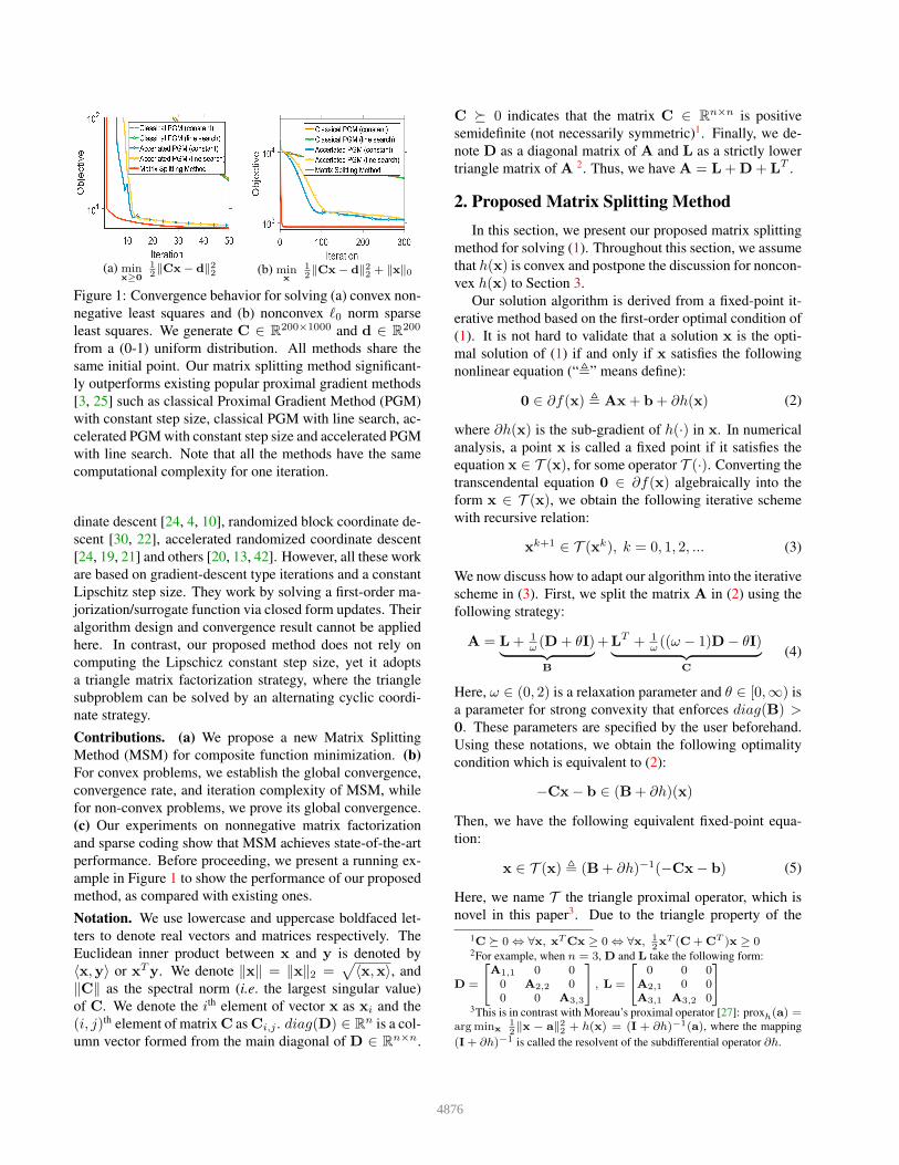
(a) minx≥0

1

2‖Cx− d‖2

2 (b) minx

1

2‖Cx− d‖2

2+ ‖x‖0

Figure 1: Convergence behavior for solving (a) convex non-

negative least squares and (b) nonconvex ℓ0 norm sparse

least squares. We generate C ∈ R200×1000 and d ∈ R

200

from a (0-1) uniform distribution. All methods share the

same initial point. Our matrix splitting method significant-

ly outperforms existing popular proximal gradient methods

[3, 25] such as classical Proximal Gradient Method (PGM)

with constant step size, classical PGM with line search, ac-

celerated PGM with constant step size and accelerated PGM

with line search. Note that all the methods have the same

computational complexity for one iteration.

dinate descent [24, 4, 10], randomized block coordinate de-

scent [30, 22], accelerated randomized coordinate descent

[24, 19, 21] and others [20, 13, 42]. However, all these work

are based on gradient-descent type iterations and a constant

Lipschitz step size. They work by solving a first-order ma-

jorization/surrogate function via closed form updates. Their

algorithm design and convergence result cannot be applied

here. In contrast, our proposed method does not rely on

computing the Lipschicz constant step size, yet it adopts

a triangle matrix factorization strategy, where the triangle

subproblem can be solved by an alternating cyclic coordi-

nate strategy.

Contributions. (a) We propose a new Matrix Splitting

Method (MSM) for composite function minimization. (b)

For convex problems, we establish the global convergence,

convergence rate, and iteration complexity of MSM, while

for non-convex problems, we prove its global convergence.

(c) Our experiments on nonnegative matrix factorization

and sparse coding show that MSM achieves state-of-the-art

performance. Before proceeding, we present a running ex-

ample in Figure 1 to show the performance of our proposed

method, as compared with existing ones.

Notation. We use lowercase and uppercase boldfaced let-

ters to denote real vectors and matrices respectively. The

Euclidean inner product between x and y is denoted by

〈x,y〉 or xTy. We denote ‖x‖ = ‖x‖2 =√

〈x,x〉, and

‖C‖ as the spectral norm (i.e. the largest singular value)

of C. We denote the ith element of vector x as xi and the

(i, j)th element of matrix C as Ci,j . diag(D) ∈ Rn is a col-

umn vector formed from the main diagonal of D ∈ Rn×n.

C � 0 indicates that the matrix C ∈ Rn×n is positive

semidefinite (not necessarily symmetric)1. Finally, we de-

note D as a diagonal matrix of A and L as a strictly lower

triangle matrix of A 2. Thus, we have A = L+D+ LT .

2. Proposed Matrix Splitting Method

In this section, we present our proposed matrix splitting

method for solving (1). Throughout this section, we assume

that h(x) is convex and postpone the discussion for noncon-

vex h(x) to Section 3.

Our solution algorithm is derived from a fixed-point it-

erative method based on the first-order optimal condition of

(1). It is not hard to validate that a solution x is the opti-

mal solution of (1) if and only if x satisfies the following

nonlinear equation (“,” means define):

0 ∈ ∂f(x) , Ax+ b+ ∂h(x) (2)

where ∂h(x) is the sub-gradient of h(·) in x. In numerical

analysis, a point x is called a fixed point if it satisfies the

equation x ∈ T (x), for some operator T (·). Converting the

transcendental equation 0 ∈ ∂f(x) algebraically into the

form x ∈ T (x), we obtain the following iterative scheme

with recursive relation:

xk+1 ∈ T (xk), k = 0, 1, 2, ... (3)

We now discuss how to adapt our algorithm into the iterative

scheme in (3). First, we split the matrix A in (2) using the

following strategy:

A = L+ 1ω (D+ θI)

︸ ︷︷ ︸

B

+LT + 1ω ((ω − 1)D− θI)

︸ ︷︷ ︸

C

(4)

Here, ω ∈ (0, 2) is a relaxation parameter and θ ∈ [0,∞) is

a parameter for strong convexity that enforces diag(B) >0. These parameters are specified by the user beforehand.

Using these notations, we obtain the following optimality

condition which is equivalent to (2):

−Cx− b ∈ (B+ ∂h)(x)

Then, we have the following equivalent fixed-point equa-

tion:

x ∈ T (x) , (B+ ∂h)−1(−Cx− b) (5)

Here, we name T the triangle proximal operator, which is

novel in this paper3. Due to the triangle property of the

1C � 0 ⇔ ∀x, xTCx ≥ 0 ⇔ ∀x, 1

2xT (C+C

T )x ≥ 02For example, when n = 3, D and L take the following form:

D =

A1,1 0 00 A2,2 00 0 A3,3

, L =

0 0 0A2,1 0 0A3,1 A3,2 0

3This is in contrast with Moreau’s proximal operator [27]: proxh(a) =argminx

1

2‖x − a‖2

2+ h(x) = (I + ∂h)−1(a), where the mapping

(I+ ∂h)−1 is called the resolvent of the subdifferential operator ∂h.

4876

matrix B and the element-wise separable structure of h(·),the triangle proximal operator T (x) in (5) can be computed

exactly and analytically, by a generalized Gaussian elimina-

tion procedure (discussed later in Section 2.1). Our matrix

splitting method iteratively applies xk+1 ⇐ T (xk) until

convergence. We summarize our algorithm in Algorithm 1.

In what follows, we show how to compute T (x) in (5) in

Section 2.1, and then we study the convergence properties

of Algorithm 1 in Section 2.2.

2.1. Computing the Triangle Proximal Operator

We now present how to compute the triangle proximal

operator in (5), which is based on a new generalized Gaus-

sian elimination procedure. Notice that (5) seeks a solution

z∗ , T (xk) that satisfies the following nonlinear system:

0 ∈ Bz∗ + u+ ∂h(z∗), where u = b+Cxk (6)

By taking advantage of the triangular form of B and the

element-wise structure of h(·), the elements of z∗ can be

computed sequentially using forward substitution. Specifi-

cally, the above equation can be written as a system of non-

linear equations:

0 ∈

B1,1 0 0 0 0B2,1 B2,2 0 0 0

.

.

....

. . . 0 0Bn−1,1 Bn−1,2 · · · Bn−1,n−1 0Bn,1 Bn,2 · · · Bn,n−1 Bn,n

z∗1

z∗2

.

.

.

z∗n−1

z∗n

+ u+ ∂h(z∗)

If z∗ satisfies the equations above, it must solve the follow-

ing one-dimensional subproblems:

0 ∈ Bj,jz∗j +wj + ∂h(z∗j ), ∀j = 1, 2, ... , n,

wj = uj +∑j−1

i=1 Bj,iz∗i

This is equivalent to solving the following one-dimensional

problem for all j = 1, 2, ..., n:

z∗j = t∗ , argmint

12Bj,jt

2 +wjt+ h(t) (7)

Note that the computation of z∗ uses only the elements of

z∗ that have already been computed and a successive dis-

placement strategy is applied to find z∗.

We remark that the one-dimensional subproblem in (7)

often admits a closed form solution for many problem-

s of interest. For example, when h(t) = I[lb,ub](t) with

I(·) denoting an indicator function on the box constrain-

t lb ≤ x ≤ ub, the optimal solution can be computed

as: t∗ = min(ub,max(lb,−wj/Bj,j)); when h(t) = λ|t|(e.g. in the case of the ℓ1 norm), the optimal solution can

be computed as: t∗ = −max (0, |wj/Bj,j | − λ/Bj,j) ·sign (wj/Bj,j).

Our generalized Gaussian elimination procedure for

computing T (xk) is summarized in Algorithm 2. Note that

its computational complexity is O(n2), which is the same

as computing a matrix-vector product.

Algorithm 1 MSM: A Matrix Splitting Method for Solving

the Composite Function Minimization Problem in (1)

1: Choose ω ∈ (0, 2), θ ∈ [0,∞). Initialize x0, k = 0.

2: while not converge

3: xk+1 = T (xk) (Solve (6) by Algorithm 2)

4: k = k + 1

5: end while

6: Output xk+1

Algorithm 2 A Generalized Gaussian Elimination Proce-

dure for Computing the Triangle Proximal Operator T (xk).

1: Input xk

2: Initialization: compute u = b+Cxk

3: x1 = argmint12B1,1t

2 + (u1)t+ h(t)

4: x2 = argmint12B2,2t

2 + (u2 +B2,1x1)t+ h(t)

5: x3 = argmint12B3,3t

2+(u3+B3,1x1+B3,2x2)t+h(t)

6: ...

7: xn = argmint12Bn,nt

2 + (un +∑n−1

i=1 Bn,ixi)t+ h(t)

8: Collect (x1,x2,x3, ...,xn)T as xk+1 and Output xk+1

2.2. Convergence Analysis

In what follows, we present our convergence analysis for

Algorithm 1. We let x∗ be the optimal solution set of (1).

For notation simplicity, we denote:

rk , xk − x∗, dk, xk+1 − xk

uk , f(xk)− f(x∗), fk , f(xk), f∗ , f(x∗)(8)

The following lemma characterizes the optimality of T (y).

Lemma 1. For all x,y ∈ Rn, it holds that:

v ∈ ∂h(T (x)), ‖AT (x) + b+ v‖ ≤ ‖C‖‖x− T (x)‖ (9)

f(T (y))− f(x) ≤ 〈T (y)− x,C(T (y)− y)

− 12 (x− T (y))TA(x− T (y))〉

(10)

Proof. (i) We now prove (9). By the optimality of T (x), we

have: ∀v ∈ ∂h(T (x)), 0 = BT (x) +CT (x) + v + b +Cx − CT (x). Therefore, we obtain: AT (x) + b + v =C(T (x)− x). Applying a norm inequality, we have (9).

(ii) We now prove (10). For simplicity, we denote z∗ ,

T (y). Thus, we obtain: 0 ∈ Bz∗ + b+Cy + ∂h(z∗) ⇒0 ∈ 〈x− z∗,Bz∗ + b+Cy+ ∂h(z∗)〉, ∀x. Since h(·) is

convex, we have:

〈x− z∗, ∂h(z∗)〉 ≤ h(x)− h(z∗) (11)

Then we have this inequality: ∀x : h(x) − h(z∗) + 〈x −z∗,Bz∗ +b+Cy〉 ≥ 0. We naturally derive the following

results: f(z∗) − f(x) = h(z∗) − h(x) + q(z∗) − q(x) ≤〈x−z∗,Bz∗+b+Cy〉+ q(z∗)− q(x) = 〈x−z∗,Bz∗+

4877

Cy〉+ 12z

∗TAz∗− 12x

TAx = 〈x−z∗, (B−A)z∗+Cy〉−12 (x − z∗)TA(x − z∗) = 〈x − z∗,C(y − z∗)〉 − 1

2 (x −z∗)TA(x− z∗).

Theorem 1. (Proof of Global Convergence) We define δ ,2θω + 2−ω

ω min(diag(D)). Assume that ω and θ are chosen

such that δ ∈ (0,∞), Algorithm 1 is globally convergent.

Proof. (i) First, the following results hold for all z ∈ Rn:

zT (A− 2C)z = zT (L− LT + 2−ωω D+ 2θ

ω I)z

= zT ( 2θω I+ 2−ωω D)z ≥ δ‖z‖22

(12)

where we have used the definition of A and C, and the fact

that zTLz = zTLT z, ∀z.

We invoke (10) in Lemma 1 with x = xk, y = xk and

combine the inequality in (12) to obtain:

fk+1 − fk ≤ − 12 〈d

k, (A− 2C)dk〉 ≤ − δ2‖d

k‖22 (13)

(ii) Second, we invoke (9) in Lemma 1 with x = xk and ob-

tain: v ∈ ∂h(xk+1), 1‖C‖‖Axk+1+b+v‖ ≤ ‖xk−xk+1‖.

Combining with (13), we have: δ‖∂f(xk+1)‖22/(2‖C‖) ≤fk − fk+1, where ∂f(xk) is defined in (2). Sum-

ming this inequality over i = 0, ..., k − 1, we have:

δ∑k−1

i=0 ‖∂f(xi)‖22/(2‖C‖) ≤ f0 − fk ≤ f0 − f∗, where

we use f∗ ≤ fk. As k → ∞, we have ∂f(xk) → 0, which

implies the convergence of the algorithm.

Note that guaranteeing δ ∈ (0,∞) can be achieved by

simply choosing ω ∈ (0, 2) and setting θ to a small number.

We now prove the convergence rate of Algorithm 1. We

make the following assumption, which characterizes the re-

lations between T (x) and x∗ for any x.

Assumption 1. If x is not the optimum of (1), there exists a

constant η ∈ (0,∞) such that ‖x− x∗‖ ≤ η‖x− T (x)‖.

We remark that this assumption is similar to the classi-

cal local proximal error bound assumption in the literature

[23, 35, 34, 41], and it is mild. Firstly, if x is not the opti-

mum, we have x 6= T (x). This is because when x = T (x),we have 0 = ‖C‖‖x−T (x)‖ ≥ ‖AT (x)+b+v‖, ∀v ∈∂h(T (x)) (refer to the optimal condition of T (x) in (9)),

which contradicts with the condition that x is not the opti-

mal solution. Secondly, by the boundedness of x and x∗,

there exists a sufficiently large constant η ∈ (0,∞) such

that ‖x− x∗‖ ≤ η‖x− T (x)‖.

We now prove the convergence rate of Algorithm 1.

Theorem 2. (Proof of Convergence Rate) We define δ ,2θω + 2−ω

ω min(diag(D)). Assume that ω and θ are chosen

such that δ ∈ (0,∞) and xk is bound for all k, we have:

f(xk+1)− f(x∗)

f(xk)− f(x∗)≤ C1

1 + C1

(14)

where C1 = ((3 + η2‖C‖ + (2η2 + 2)‖A‖)/δ. In other

words, Algorithm 1 converges to the optimal solution Q-

linearly.

Proof. Invoking Assumption 1 with x = xk, we obtain:

‖xk − x∗‖ ≤ η‖xk − T (xk)‖ ⇒ ‖rk‖ ≤ η‖dk‖ (15)

Invoking (10) in Lemma 1 with x = x∗, y = xk, we derive

the following inequalities:

fk+1 − f∗

≤ 〈rk+1,Cdk〉 − 12 〈rk+1,Ark+1〉

= 〈rk + dk,Cdk〉 − 12 〈rk + dk,A(rk + dk)〉

≤ ‖C‖(‖dk‖‖rk‖+ ‖dk‖22) + 12‖A‖‖rk + dk‖22

≤ ‖C‖( 32‖dk‖22 + 1

2‖rk‖22) + ‖A‖(‖rk‖22 + ‖dk‖22)≤ ‖C‖ 3+η2

2 ‖dk‖22 + ‖A‖(η2 + 1)‖dk‖22≤ ((3 + η2‖C‖+ (2η2 + 2)‖A‖) · (fk − fk+1)/δ

= C1(fk − fk+1)

= C1(fk − f∗)− C1(f

k+1 − f∗)

(16)

where the second step uses the fact that rk+1 = rk + dk;

the third step uses the Cauchy-Schwarz inequality 〈x,y〉 ≤‖x‖‖y‖, ∀x,y ∈ R

n and the norm inequality ‖Ax‖ ≤‖A‖‖x‖, ∀x ∈ R

n; the fourth step uses the fact that 1/2 ·‖x + y‖22 ≤ ‖x‖22 + ‖y‖22, ∀x,y ∈ R

n and ab ≤ 1/2 ·a2 + 1/2 · b2, ∀a, b ∈ R; the fifth step uses (15); the sixth

step uses the descent condition in (13). Rearranging the last

inequality in (16), we have (1 + C1)f(xk+1) − f(x∗) ≤

C1(f(xk)− f(x∗)) and obtain the inequality in (14). Since

C1

1+C1< 1, the sequence {f(xk)}∞k=0 converges to f(x∗)

linearly in the quotient sense.

The following lemma is useful in our proof of iteration

complexity.

Lemma 2. Suppose a nonnegative sequence {uk}∞k=0 satis-

fies uk+1 ≤ −2C +2C√

1 + uk

C for some constant C ≥ 0.

It holds that: uk+1 ≤ C2

k+1 , where C2 = max(8C, 2√Cu0).

Proof. The proof of this lemma can be obtained by mathe-

matical induction. (i) When k = 0, we have u1 ≤ −2C +

2C√

1 + 1Cu0 ≤ −2C+2C(1+

√u0

C ) = 2√Cu0 ≤ C0

k+1 .

(ii) When k ≥ 1, we assume that uk ≤ C2

k holds. We derive

the following results: k ≥ 1 ⇒ k+1k ≤ 2 ⇒ 4C k+1

k ≤8C ≤ C2 ⇒ 4C

k(k+1) = 4C( 1k − 1k+1 ) ≤

C2

(k+1)2 ⇒ 4Ck ≤

4Ck+1 + C2

(k+1)2 ⇒ 4C2(1 + C2

kC ) ≤ 4C2 + 4CC2

k+1 +C2

2

(k+1)2

⇒ 2C√

1 + C2

Ck ≤ 2C + C2

k+1 ⇒ −2C + 2C√

1 + C2

Ck ≤C2

k+1 ⇒ −2C + 2C√

1 + uk

C ≤ C2

k+1 ⇒ uk+1 ≤ C2

k+1 .

4878

We now prove the iteration complexity of Algorithm 1.

Theorem 3. (Proof of Iteration Complexity) We define δ ,2θω + 2−ω

ω min(diag(D)). Assume that ω and θ are chosen

such that δ ∈ (0,∞) and ‖xk‖ ≤ R, ∀k, we have:

uk ≤{

u0( 2C4

2C4+1 )k, if

√

fk − fk+1 ≥ C3/C4, ∀k ≤ kC5

k , if√

fk − fk+1 < C3/C4, ∀k ≥ 0

where C3 = 2R‖C‖( δ2 )1/2, C4 = δ2 (‖C‖+ ‖A‖(η + 1)),

C5 = max(8C23 , 2C3

√u0), and k is some unknown itera-

tion index.

Proof. Using similar strategies used in deriving (16), we

have the following results:

uk+1

≤ 〈rk+1,Cdk〉 − 12 〈rk+1,Ark+1〉

= 〈rk + dk,Cdk〉 − 12 〈rk + dk,A(rk + dk)〉

≤ ‖C‖(‖rk‖‖dk‖+ ‖dk‖22) + ‖A‖2 ‖rk + dk‖22

≤ ‖C‖(‖rk‖‖dk‖+ ‖dk‖22) + ‖A‖(‖rk‖22 + ‖dk‖22)≤ ‖C‖(2R‖dk‖+ ‖dk‖22) + ‖A‖(η‖dk‖22 + ‖dk‖22)≤ C3

√

uk − uk+1 + C4(uk − uk+1)

(17)

Now we consider the two cases for the recursion formu-

la in (17): (i)√uk − uk+1 ≥ C3

C4for some k ≤ k (i-

i)√uk − uk+1 ≤ C3

C4for all k ≥ 0. In case (i), (17)

implies that we have uk+1 ≤ 2C4(uk − uk+1) and rear-

ranging terms gives: uk+1 ≤ 2C4

2C4+1uk. Thus, we have:

uk+1 ≤ ( 2C4

2C4+1 )k+1u0. We now focus on case (ii). When√

uk − uk+1 ≤ C3

C4, (17) implies that we have uk+1 ≤

2C3

√uk − uk+1 and rearranging terms yields:

(uk+1)2

4C23

+

uk+1 ≤ uk. Solving this quadratic inequality, we have:

uk+1 ≤ −2C23 + 2C2

3

√

1 + 1C2

3

uk; solving this recursive

formulation by Lemma 2, we obtain uk+1 ≤ C5

k+1 .

We have a few comments on Algorithm 1. (i) When h(·)is empty and θ = 0, it reduces to the classical Gauss-Seidel

method (ω = 1) and Successive Over-Relaxation method

(ω 6= 1). (ii) When A contains zeros in its diagonal en-

tries, one needs to set θ to a strictly positive number. This

is to guarantee the strong convexity of the one dimensional

subproblem and a bounded solution for any h(·). We re-

mark that the introduction of the parameter θ is novel in

this paper and it removes the assumption that A is strictly

positive-definite or strictly diagonally dominant, which is

used in the classical result of GS and SOC method [31, 6].

3. Extensions

This section discusses several extensions of our proposed

matrix splitting method for solving (1).

3.1. When h is Nonconvex

When h(x) is nonconvex, our theoretical analysis breaks

down in (11) and the exact solution to the triangle proximal

operator T (xk) in (6) cannot be guaranteed. However, our

Gaussian elimination procedure in Algorithm 2 can still be

applied. What one needs is to solve a one-dimensional non-

convex subproblem in (7). For example, when h(t) = λ|t|0(e.g. in the case of the ℓ0 norm), it has an analytical solu-

tion: t∗ ={

−wj/Bj,j , w2j > 2λBj,j

0, w2j ≤ 2λBj,j

; when h(t) = λ|t|pand p < 1, it admits a closed form solution for some special

values [36], such as p = 12 or 2

3 .

Our matrix splitting method is guaranteed to converge

even when h(·) is nonconvex. Specifically, we present the

following theorem.

Theorem 4. (Proof of Global Convergence when h(·) is

Nonconvex) Assume the nonconvex one-dimensional sub-

problem in (7) can be solved globally and analytically.

We define δ , min (θ/ω + (1− ω)/ω · diag(D)). If we

choose ω and θ such that δ ∈ (0,∞), we have: (i)

f(xk+1)− f(xk) ≤ − δ2‖xk+1 − xk‖22 ≤ 0 (18)

(ii) Algorithm 1 is globally convergent.

Proof. (i) Due to the optimality of the one-dimensional sub-

problem in (7), for all j = 1, 2, ..., n, we have:

12Bj,j(x

k+1j )2 + (uj +

∑j−1i=1 Bj,ix

k+1i )xk+1

j + h(xk+1j )

≤ 12Bj,jt

2j + (uj +

∑j−1i=1 Bj,ix

k+1i )tj + h(tj), ∀tj

Letting t1 = xk1 , t2 = xk

2 , ... , tn = xkn, we obtain:

12

∑ni Bi,i(x

k+1i )2 + 〈u+ Lxk+1,xk+1〉+ h(xk+1)

≤ 12

∑ni Bi,i(x

ki )

2 + 〈u+ Lxk+1,xk〉+ h(xk)

Since u = b+Cxk, we obtain the following inequality:

fk+1 + 12 〈xk+1, ( 1

ω (D+ θI) + 2L−A)xk+1 + 2Cxk〉≤ fk + 1

2 〈xk, ( 1

ω (D+ θI) + 2C−A)xk + 2Lxk+1〉

By denoting S , L−LT and T , ((ω−1)D− θI)/ω, we

have: 1ω (D+ θI) + 2L−A = T−S, 1

ω (D+ θI) + 2C−A = S − T, and L −CT = −T. Therefore, we have the

following inequalities:

fk+1 − fk ≤ 12 〈xk+1, (T− S)xk+1〉 − 〈xk,Txk+1)

+ 12 〈xk, (T− S)xk〉 = 1

2 〈xk − xk+1,T(xk − xk+1)〉≤ − δ

2‖xk+1 − xk‖22

4879

where the first equality uses 〈x,Sx〉 = 0 ∀x, since S is a

Skew-Hermitian matrix. The last step uses T + δI � 0,

since x+min(−x) ≤ 0 ∀x. Thus, we obtain the sufficient

decrease inequality in (18).

(ii) Based on the sufficient decrease inequality in (18),

we have: f(xk) is a non-increasing sequence, ‖xk −xk+1‖ → 0, and f(xk+1) < f(xk) if xk 6= xk+1. We note

that (9) can be still applied even h(·) is nonconvex. Using

the same methodology as in the second part of Theorem 1,

we obtain that ∂f(xk) → 0, which implies the convergence

of the algorithm.

Note that guaranteeing δ ∈ (0,∞) can be achieved by

simply choosing ω ∈ (0, 1) and setting θ to a small number.

3.2. When x is a Matrix

In many applications (e.g. nonegative matrix factoriza-

tion and sparse coding), the solutions exist in the matrix

form as follows: minX∈Rn×r12 tr(X

TAX)+ tr(XTR)+h(X), where R ∈ R

n×r. Our matrix splitting algorith-

m can still be applied in this case. Using the same tech-

nique to decompose A as in (4): A = B + C, one need-

s to replace (6) to solve the following nonlinear equation:

BZ∗ +U+ ∂h(Z∗) ∈ 0, where U = R+CXk. It can be

decomposed into r independent components. By updating

every column of X, the proposed algorithm can be used to

solve the matrix problem above. Thus, our algorithm can al-

so make good use of existing parallel architectures to solve

the matrix optimization problem.

3.3. When q is not Quadratic

Since the second-order Taylor series is a majorizer of

any twice differentiable convex function q(x) (not necessar-

ily quadratic), the following inequality always holds [15]:

q(y) ≤ Q(y,x) , q(x) + 〈∇q(x),y − x〉 + 12 (y −

x)TM(y − x) for any x and y such that M ≻ ∇q2(x),where ∇q(x) and ∇2q(x) denote the gradient and Hes-

sian of q(x) at x, respectively. By minimizing (approxi-

mately) the upper bound of q(y) (i.e. the quadratic sur-

rogate function) at the current estimate x, i.e. xk+1 =argminy Q(y,xk) + h(y), we can drive the objective

downward until a stationary point is reached. In addi-

tion, one can perform line search by the update [35, 40]:

xk+1 ⇐ xk + β(xk+1 − xk) for the greatest descen-

t in objective (as in the damped Newton method). Here,

β ∈ (0, 1] is the step-size selected by backtracking line

search. Note that classical proximal point method consid-

ers M = ||∇q2(x)|| · I, while we can consider the lower

triangle matrix of ∇q2(x) in our algorithm.

4. Experiments

This section demonstrates the efficiency and efficacy of

the proposed Matrix Splitting Method (MSM) by consider-

ing two important applications: nonnegative matrix factor-

ization (NMF) [16, 18] and cardinality regularized sparse

coding [26, 29, 17]. We implement our method in MAT-

LAB on an Intel 2.6 GHz CPU with 8 GB RAM. Only our

generalized Gaussian elimination procedure is developed in

C and wrapped into the MATLAB code, since it requires

an elementwise loop that is quite inefficient in native MAT-

LAB. We report our results with the choice θ = 0.01 and

ω = 1 in all our experiments. Some Matlab code can be

found in the authors’ research webpages.

4.1. Nonnegative Matrix Factorization (NMF)

Nonnegative matrix factorization [16] is a very useful

tool for feature extraction and identification in the fields of

text mining and image understanding. It is formulated as

the following optimization problem:

minW,H

12‖Y −WH‖2F , s.t. W ≥ 0, H ≥ 0 (19)

where W ∈ Rm×n and H ∈ R

n×d. Following previous

work [14, 9, 18, 12], we alternatively minimize the objec-

tive while keeping one of the two variables fixed. In each al-

ternating subproblem, we solve a convex nonnegative least

squares problem, where our MSM method is used. We con-

duct experiments on three datasets 4 20news, COIL, and T-

DT2. The size of the datasets are 18774 × 61188, 7200 ×1024, 9394 × 36771, respectively. We compare MSM a-

gainst the following state-of-the-art methods: (1) Projec-

tive Gradient (PG) [18, 5] that updates the current solution

via steep gradient descent and then maps a point back to

the bounded feasible region 5; (2) Active Set (AS) method

[14]; (3) Block Principal Pivoting (BPP) method [14] 6 that

iteratively identifies an active and passive set by a princi-

pal pivoting procedure and solves a reduced linear system;

(4) Accelerated Proximal Gradient (APG) [9] 7 that applies

Nesterov’s momentum strategy with a constant step size

to solve the convex sub-problems; (5) Coordinate Gradi-

ent Descent (CGD) [12] 8 that greedily selects one coor-

dinate by measuring the objective reduction and optimizes

for a single variable via closed-form update. Similar to our

method, the core procedure of CGD is developed in C and

wrapped into the MATLAB code, while all other methods

are implemented using builtin MATLAB functions.

We use the same settings as in [18]. We compare objec-

tive values after running t seconds with t varying from 20

to 50. Table 1 presents average results of using 10 random

initial points, which are generated from a standard normal

distribution. While the other methods may quickly lower

4http://www.cad.zju.edu.cn/home/dengcai/Data/TextData.html5https://www.csie.ntu.edu.tw/∼cjlin/libmf/6http://www.cc.gatech.edu/∼hpark/nmfsoftware.php7https://sites.google.com/site/nmfsolvers/8http://www.cs.utexas.edu/∼cjhsieh/nmf/

4880

data n [18] [14] [14] [9] [12] [ours]

PG AS BPP APG CGD MSM

time limit=20

20news 20 5.001e+06 2.762e+07 8.415e+06 4.528e+06 4.515e+06 4.506e+06

20news 50 5.059e+06 2.762e+07 4.230e+07 3.775e+06 3.544e+06 3.467e+06

20news 100 6.955e+06 5.779e+06 4.453e+07 3.658e+06 3.971e+06 2.902e+06

20news 200 7.675e+06 3.036e+06 1.023e+08 4.431e+06 3.573e+07 2.819e+06

20news 300 1.997e+07 2.762e+07 1.956e+08 4.519e+06 4.621e+07 3.202e+06

COIL 20 2.004e+09 5.480e+09 2.031e+09 1.974e+09 1.976e+09 1.975e+09

COIL 50 1.412e+09 1.516e+10 6.962e+09 1.291e+09 1.256e+09 1.252e+09

COIL 100 2.960e+09 2.834e+10 3.222e+10 9.919e+08 8.745e+08 8.510e+08

COIL 200 3.371e+09 2.834e+10 5.229e+10 8.495e+08 5.959e+08 5.600e+08

COIL 300 3.996e+09 2.834e+10 1.017e+11 8.493e+08 5.002e+08 4.956e+08

TDT2 20 1.597e+06 2.211e+06 1.688e+06 1.591e+06 1.595e+06 1.592e+06

TDT2 50 1.408e+06 2.211e+06 2.895e+06 1.393e+06 1.390e+06 1.385e+06

TDT2 100 1.300e+06 2.211e+06 6.187e+06 1.222e+06 1.224e+06 1.214e+06

TDT2 200 1.628e+06 2.211e+06 1.791e+07 1.119e+06 1.227e+06 1.079e+06

TDT2 300 1.915e+06 1.854e+06 3.412e+07 1.172e+06 7.902e+06 1.066e+06

time limit=30

20news 20 4.716e+06 2.762e+07 7.471e+06 4.510e+06 4.503e+06 4.500e+06

20news 50 4.569e+06 2.762e+07 5.034e+07 3.628e+06 3.495e+06 3.446e+06

20news 100 6.639e+06 2.762e+07 4.316e+07 3.293e+06 3.223e+06 2.817e+06

20news 200 6.991e+06 2.762e+07 1.015e+08 3.609e+06 7.676e+06 2.507e+06

20news 300 1.354e+07 2.762e+07 1.942e+08 4.519e+06 4.621e+07 3.097e+06

COIL 20 1.992e+09 4.405e+09 2.014e+09 1.974e+09 1.975e+09 1.975e+09

COIL 50 1.335e+09 2.420e+10 5.772e+09 1.272e+09 1.252e+09 1.250e+09

COIL 100 2.936e+09 2.834e+10 1.814e+10 9.422e+08 8.623e+08 8.458e+08

COIL 200 3.362e+09 2.834e+10 4.627e+10 7.614e+08 5.720e+08 5.392e+08

COIL 300 3.946e+09 2.834e+10 7.417e+10 6.734e+08 4.609e+08 4.544e+08

TDT2 20 1.595e+06 2.211e+06 1.667e+06 1.591e+06 1.594e+06 1.592e+06

TDT2 50 1.397e+06 2.211e+06 2.285e+06 1.393e+06 1.389e+06 1.385e+06

TDT2 100 1.241e+06 2.211e+06 5.702e+06 1.216e+06 1.219e+06 1.212e+06

TDT2 200 1.484e+06 1.878e+06 1.753e+07 1.063e+06 1.104e+06 1.049e+06

TDT2 300 1.879e+06 2.211e+06 3.398e+07 1.060e+06 1.669e+06 1.007e+06

data n [18] [14] [14] [9] [12] [ours]

PG AS BPP APG CGD MSM

time limit=40

20news 20 4.622e+06 2.762e+07 7.547e+06 4.495e+06 4.500e+06 4.496e+06

20news 50 4.386e+06 2.762e+07 1.562e+07 3.564e+06 3.478e+06 3.438e+06

20news 100 6.486e+06 2.762e+07 4.223e+07 3.128e+06 2.988e+06 2.783e+06

20news 200 6.731e+06 1.934e+07 1.003e+08 3.304e+06 5.744e+06 2.407e+06

20news 300 1.041e+07 2.762e+07 1.932e+08 3.621e+06 4.621e+07 2.543e+06

COIL 20 1.987e+09 5.141e+09 2.010e+09 1.974e+09 1.975e+09 1.975e+09

COIL 50 1.308e+09 2.403e+10 5.032e+09 1.262e+09 1.250e+09 1.248e+09

COIL 100 2.922e+09 2.834e+10 2.086e+10 9.161e+08 8.555e+08 8.430e+08

COIL 200 3.361e+09 2.834e+10 4.116e+10 7.075e+08 5.584e+08 5.289e+08

COIL 300 3.920e+09 2.834e+10 7.040e+10 6.221e+08 4.384e+08 4.294e+08

TDT2 20 1.595e+06 2.211e+06 1.643e+06 1.591e+06 1.594e+06 1.592e+06

TDT2 50 1.394e+06 2.211e+06 1.933e+06 1.392e+06 1.388e+06 1.384e+06

TDT2 100 1.229e+06 2.211e+06 5.259e+06 1.213e+06 1.216e+06 1.211e+06

TDT2 200 1.389e+06 1.547e+06 1.716e+07 1.046e+06 1.070e+06 1.041e+06

TDT2 300 1.949e+06 1.836e+06 3.369e+07 1.008e+06 1.155e+06 9.776e+05

time limit=50

20news 20 4.565e+06 2.762e+07 6.939e+06 4.488e+06 4.498e+06 4.494e+06

20news 50 4.343e+06 2.762e+07 1.813e+07 3.525e+06 3.469e+06 3.432e+06

20news 100 6.404e+06 2.762e+07 3.955e+07 3.046e+06 2.878e+06 2.765e+06

20news 200 5.939e+06 2.762e+07 9.925e+07 3.121e+06 4.538e+06 2.359e+06

20news 300 9.258e+06 2.762e+07 1.912e+08 3.621e+06 2.323e+07 2.331e+06

COIL 20 1.982e+09 7.136e+09 2.033e+09 1.974e+09 1.975e+09 1.975e+09

COIL 50 1.298e+09 2.834e+10 4.365e+09 1.258e+09 1.248e+09 1.248e+09

COIL 100 1.945e+09 2.834e+10 1.428e+10 9.014e+08 8.516e+08 8.414e+08

COIL 200 3.362e+09 2.834e+10 3.760e+10 6.771e+08 5.491e+08 5.231e+08

COIL 300 3.905e+09 2.834e+10 6.741e+10 5.805e+08 4.226e+08 4.127e+08

TDT2 20 1.595e+06 2.211e+06 1.622e+06 1.591e+06 1.594e+06 1.592e+06

TDT2 50 1.393e+06 2.211e+06 1.875e+06 1.392e+06 1.386e+06 1.384e+06

TDT2 100 1.223e+06 2.211e+06 4.831e+06 1.212e+06 1.214e+06 1.210e+06

TDT2 200 1.267e+06 2.211e+06 1.671e+07 1.040e+06 1.054e+06 1.036e+06

TDT2 300 1.903e+06 2.211e+06 3.328e+07 9.775e+05 1.045e+06 9.606e+05

Table 1: Comparisons of objective values for non-negative matrix factorization for all the compared methods. The 1st, 2nd,

and 3rd best results are colored with red, blue and green, respectively.

objective values when n is small (n = 20), MSM catch-

es up very quickly and achieves a faster convergence speed

when n is large. It generally achieves the best performance

in terms of objective value among all the methods.

4.2. Cardinality Regularized Sparse Coding

Sparse coding is a popular unsupervised feature learn-

ing technique for data representation that is widely used in

computer vision and medical imaging. Motivated by recent

success in ℓ0 norm modeling [39, 2, 37], we consider the

following cardinality regularized (i.e. ℓ0 norm) sparse cod-

ing problem:

minW,H

12‖Y −WH‖2F + λ‖H‖0, s.t. ‖W(:, i)‖2 = 1 ∀i (20)

with W ∈ Rm×n and H ∈ R

n×d. Existing solutions for

this problem are mostly based on the family of proximal

point methods [25, 2]. We compare MSM with the follow-

ing methods: (1) Proximal Gradient Method (PGM) with

constant step size, (2) PGM with line search, (3) accelerat-

ed PGM with constant step size, and (4) accelerated PGM

with line search.

We evaluate all the methods for the application of im-

age denoising. Following [1, 2], we set the dimension

of the dictionary to n = 256. The dictionary is learned

from m = 1000 image patches randomly chosen from

the noisy input image. The patch size is 8 × 8, leading

to d = 64. The experiments are conducted on 16 con-

ventional test images with different noise standard devia-

tions σ. For the regulization parameter λ, we sweep over

{1, 3, 5, 7, 9, ..., 10000, 30000, 50000, 70000, 90000}.

First, we compare the objective values for all methods by

fixing the variable W to an over-complete DCT dictionary

[1] and only optimizing over H. We compare all methods

with varying regularization parameter λ and different initial

points that are either generated by random Gaussian sam-

pling or the Orthogonal Matching Pursuit (OMP) method

[33]. In Figure 2, we observe that MSM converges rapidly

in 10 iterations. Moreover, it often generates much better

local optimal solutions than the compared methods.

Second, we evaluate the methods according to Signal-

to-Noise Ratio (SNR) value wrt the groundtruth denoised

image. In this case, we minimize over W and H alternat-

ingly with different initial points (OMP initialization or s-

tandard normal random initialization). For updating W, we

use the same proximal gradient method as in [2]. For up-

dating H, since the accelerated PGM does not necessarily

present better performance than canonical PGM and since

the line search strategy does not present better performance

than the simple constant step size, we only compare with

PGM, which has been implemented in [2] 9 and KSVD [1]10. In our experiments, we find that MSM achieves lower

9Code: http://www.math.nus.edu.sg/∼matjh/research/research.htm10Code: http://www.cs.technion.ac.il/∼elad/software/

4881

(a) λ = 5 (b) λ = 50 (c) λ = 500 (d) λ = 5000 (e) λ = 50000

(f) λ = 5 (g) λ = 50 (h) λ = 500 (i) λ = 5000 (j) λ = 50000

(k) λ = 5 (l) λ = 50 (m) λ = 500 (n) λ = 5000 (o) λ = 50000

Figure 2: Convergence behavior for solving (20) with fixing W for different λ and initializations. Denoting O as an arbitrary

standard Gaussian random matrix of suitable size, we consider the following three initializations for H. First row: H =0.1× O. Second row: H = 10× O. Third row: H is set to the output of the orthogonal matching pursuit.

OMP init random init

img + σ KSVD PGM MSM PGM MSM

walkbridge + 5 35.70 35.71 35.71 35.72 35.75

walkbridge + 10 31.07 31.07 31.17 31.07 31.17

walkbridge + 20 27.01 27.11 27.21 27.07 27.23

walkbridge + 30 24.93 25.08 25.21 25.09 25.19

walkbridge + 40 23.71 23.85 23.87 23.84 23.90

mandrill + 5 35.18 35.21 35.20 35.22 35.21

mandrill + 10 30.36 30.38 30.47 30.38 30.47

mandrill + 20 26.02 26.15 26.31 26.12 26.33

mandrill + 30 23.75 23.96 24.19 23.96 24.18

mandrill + 40 22.37 22.61 22.78 22.57 22.81

livingroom + 5 37.00 36.97 37.10 36.94 37.07

livingroom + 10 32.98 33.02 33.19 32.92 33.27

livingroom + 20 29.22 29.16 29.55 29.23 29.57

livingroom + 30 27.04 27.04 27.43 27.06 27.45

livingroom + 40 25.62 25.55 25.78 25.59 25.81

OMP init random init

img + σ KSVD PGM MSM PGM MSM

lake + 5 36.77 36.74 36.77 36.73 36.75

lake + 10 32.84 32.75 32.86 32.77 32.90

lake + 20 29.32 29.19 29.36 29.23 29.38

lake + 30 27.32 27.04 27.30 27.10 27.33

lake + 40 25.94 25.66 25.80 25.59 25.80

blonde + 5 36.98 37.00 37.06 37.00 37.08

blonde + 10 33.23 33.31 33.37 33.27 33.43

blonde + 20 29.83 29.78 29.99 29.75 30.00

blonde + 30 28.00 27.77 28.04 27.73 27.95

blonde + 40 26.82 26.33 26.41 26.31 26.63

barbara + 5 37.50 37.46 37.74 37.42 37.71

barbara + 10 33.36 33.37 33.65 33.33 33.67

barbara + 20 29.19 29.22 29.70 29.30 29.63

barbara + 30 26.79 26.84 27.30 26.92 27.36

barbara + 40 25.11 25.02 25.71 25.16 25.83

OMP init random init

img + σ KSVD PGM MSM PGM MSM

boat + 5 36.94 36.94 36.98 36.93 37.01

boat + 10 33.10 33.02 33.24 33.05 33.31

boat + 20 29.47 29.40 29.66 29.52 29.65

boat + 30 27.50 27.27 27.50 27.29 27.52

boat + 40 26.16 25.84 26.13 25.86 26.03

pirate + 5 36.49 36.43 36.54 36.42 36.50

pirate + 10 32.19 32.09 32.25 32.10 32.29

pirate + 20 28.33 28.23 28.42 28.24 28.44

pirate + 30 26.31 26.12 26.28 26.13 26.33

pirate + 40 24.94 24.71 24.86 24.72 24.86

jetplane + 5 38.84 38.87 39.06 38.93 39.05

jetplane + 10 34.98 34.99 35.17 35.01 35.22

jetplane + 20 31.30 31.04 31.28 31.01 31.30

jetplane + 30 29.11 28.64 28.87 28.68 28.95

jetplane + 40 27.57 27.05 27.19 26.97 27.26

Table 2: Comparisons of SNR values for the sparse coding based image denoising problem with OMP initialization and

random initialization. The 1st, 2nd, and 3rd best results are colored with red, blue and green, respectively.

objectives than PGM in all cases. We do not report the ob-

jective values here but only the best SNR value, since (i)

the best SNR result does not correspond to the same λ for

PGM and MSM, and (ii) KSVD does not solve exactly the

same problem in (20)11. We observe that MSM is general-

ly 4-8 times faster than KSVD. This is not surprising, since

KSVD needs to call OMP to update the dictionary H, which

11In fact, it solves an ℓ0 norm constrained problem using a greedy pur-

suit algorithm and performs a codebook update using SVD. It may not nec-

essarily converge, which motivates the use of the alternating minimization

algorithm in [2].

involves high computational complexity while our method

only needs to call a generalized Gaussian elimination proce-

dure in each iteration. In Table 2, we summarize the results,

from which we make two conclusions. (i) The two initial-

ization strategies generally lead to similar SNR results. (ii)

Our MSM method generally leads to a larger SNR than PG-

M and a comparable SNR as KSVD, but in less time.

Acknowledgments. This work was supported by the King

Abdullah University of Science and Technology (KAUST)

Office of Sponsored Research and, in part, by the NSF-

China (61402182, 61472456, 61522115, 61628212).

4882

References

[1] M. Aharon, M. Elad, and A. Bruckstein. K-svd: An

algorithm for designing overcomplete dictionaries for

sparse representation. IEEE Transactions on Signal

Processing, 54(11):4311–4322, 2006. 1, 7

[2] C. Bao, H. Ji, Y. Quan, and Z. Shen. Dictionary

learning for sparse coding: Algorithms and conver-

gence analysis. IEEE Transactions on Pattern Anal-

ysis and Machine Intelligence (TPAMI), 38(7):1356–

1369, 2016. 1, 7, 8

[3] A. Beck and M. Teboulle. A fast iterative shrinkage-

thresholding algorithm for linear inverse problem-

s. SIAM Journal on Imaging Sciences (SIIMS),

2(1):183–202, 2009. 1, 2

[4] A. Beck and L. Tetruashvili. On the convergence of

block coordinate descent type methods. SIAM journal

on Optimization (SIOPT), 23(4):2037–2060, 2013. 2

[5] D. P. Bertsekas. Nonlinear programming. Athena sci-

entific Belmont, 1999. 6

[6] J. W. Demmel. Applied numerical linear algebra.

SIAM, 1997. 1, 5

[7] D. L. Donoho. Compressed sensing. IEEE Transac-

tions on Information Theory, 52(4):1289–1306, 2006.

1

[8] E. Elhamifar and R. Vidal. Sparse subspace cluster-

ing: Algorithm, theory, and applications. IEEE Trans-

actions on Pattern Analysis and Machine Intelligence

(TPAMI), 35(11):2765–2781, 2013. 1

[9] N. Guan, D. Tao, Z. Luo, and B. Yuan. Nenmf: an

optimal gradient method for nonnegative matrix fac-

torization. IEEE Transactions on Signal Processing,

60(6):2882–2898, 2012. 1, 6, 7

[10] M. Hong, X. Wang, M. Razaviyayn, and Z.-Q. Lu-

o. Iteration complexity analysis of block coordinate

descent methods. Mathematical Programming, pages

1–30, 2013. 2

[11] C.-J. Hsieh, K.-W. Chang, C.-J. Lin, S. S. Keerthi, and

S. Sundararajan. A dual coordinate descent method for

large-scale linear svm. In International Conference on

Machine Learning (ICML), pages 408–415, 2008. 1

[12] C.-J. Hsieh and I. S. Dhillon. Fast coordinate de-

scent methods with variable selection for non-negative

matrix factorization. In ACM SIGKDD International

Conference on Knowledge Discovery and Data Min-

ing (SIGKDD), pages 1064–1072, 2011. 6, 7

[13] R. Johnson and T. Zhang. Accelerating stochastic gra-

dient descent using predictive variance reduction. In

Advances in Neural Information Processing Systems

(NIPS), pages 315–323, 2013. 2

[14] J. Kim and H. Park. Fast nonnegative matrix factor-

ization: An active-set-like method and comparison-

s. SIAM Journal on Scientific Computing (SISC),

33(6):3261–3281, 2011. 6, 7

[15] K. Lange, D. R. Hunter, and I. Yang. Optimization

transfer using surrogate objective functions. Journal

of Computational and Graphical Statistics, 9(1):1–20,

2000. 6

[16] D. D. Lee and H. S. Seung. Learning the parts of

objects by non-negative matrix factorization. Nature,

401(6755):788–791, 1999. 1, 6

[17] H. Lee, A. Battle, R. Raina, and A. Y. Ng. Efficient

sparse coding algorithms. In Advances in Neural In-

formation Processing Systems (NIPS), pages 801–808,

2006. 1, 6

[18] C.-J. Lin. Projected gradient methods for non-

negative matrix factorization. Neural Computation,

19(10):2756–2779, 2007. 1, 6, 7

[19] Q. Lin, Z. Lu, and L. Xiao. An accelerated randomized

proximal coordinate gradient method and its applica-

tion to regularized empirical risk minimization. SIAM

Journal on Optimization (SIOPT), 25(4):2244–2273,

2015. 2

[20] J. Liu and S. J. Wright. Asynchronous stochas-

tic coordinate descent: Parallelism and convergence

properties. SIAM Journal on Optimization (SIOPT),

25(1):351–376, 2015. 2

[21] Z. Lu and L. Xiao. Randomized block coordinate

non-monotone gradient method for a class of nonlin-

ear programming. arXiv preprint, 2013. 2

[22] Z. Lu and L. Xiao. On the complexity analysis of ran-

domized block-coordinate descent methods. Mathe-

matical Programming, 152(1-2):615–642, 2015. 2

[23] Z.-Q. Luo and P. Tseng. Error bounds and conver-

gence analysis of feasible descent methods: a general

approach. Annals of Operations Research, 46(1):157–

178, 1993. 4

[24] Y. Nesterov. Efficiency of coordinate descent methods

on huge-scale optimization problems. SIAM Journal

on Optimization (SIOPT), 22(2):341–362, 2012. 2

[25] Y. Nesterov. Introductory lectures on convex optimiza-

tion: A basic course, volume 87. Springer Science &

Business Media, 2013. 1, 2, 7

[26] B. A. Olshausen et al. Emergence of simple-cell re-

ceptive field properties by learning a sparse code for

natural images. Nature, 381(6583):607–609, 1996. 6

[27] N. Parikh, S. P. Boyd, et al. Proximal algorithm-

s. Foundations and Trends in optimization, 1(3):127–

239, 2014. 2

4883

[28] A. Patrascu and I. Necoara. Iteration complexity anal-

ysis of random coordinate descent methods for ℓ0 reg-

ularized convex problems. arXiv preprint, 2014. 1

[29] Y. Quan, Y. Xu, Y. Sun, Y. Huang, and H. Ji. Sparse

coding for classification via discrimination ensemble.

In IEEE Conference on Computer Vision and Pattern

Recognition (CVPR), June 2016. 1, 6

[30] P. Richtarik and M. Takac. Iteration complexity of ran-

domized block-coordinate descent methods for mini-

mizing a composite function. Mathematical Program-

ming, 144(1-2):1–38, 2014. 2

[31] Y. Saad. Iterative Methods for Sparse Linear System-

s. Society for Industrial and Applied Mathematics,

Philadelphia, PA, USA, 2nd edition, 2003. 1, 5

[32] R. Sun and M. Hong. Improved iteration complexity

bounds of cyclic block coordinate descent for convex

problems. In Advances in Neural Information Pro-

cessing Systems (NIPS), pages 1306–1314, 2015. 1

[33] J. A. Tropp and A. C. Gilbert. Signal recovery

from random measurements via orthogonal matching

pursuit. IEEE Transactions on Information Theory,

53(12):4655–4666, 2007. 7

[34] P. Tseng. Approximation accuracy, gradient methods,

and error bound for structured convex optimization.

Mathematical Programming, 125(2):263–295, 2010.

4

[35] P. Tseng and S. Yun. A coordinate gradient descent

method for nonsmooth separable minimization. Math-

ematical Programming, 117(1-2):387–423, 2009. 1, 4,

6

[36] Z. Xu, X. Chang, F. Xu, and H. Zhang. L1/2 regu-

larization: A thresholding representation theory and a

fast solver. IEEE Transactions on Neural Network-

s and Learning Systems (TNNLS), 23(7):1013–1027,

2012. 5

[37] Y. Yang, J. Feng, N. Jojic, J. Yang, and T. S. Huang.

ℓ0-sparse subspace clustering. European Conference

on Computer Vision (ECCV), 2016. 7

[38] H.-F. Yu, F.-L. Huang, and C.-J. Lin. Dual coordinate

descent methods for logistic regression and maximum

entropy models. Machine Learning, 85(1-2):41–75,

2011. 1

[39] G. Yuan and B. Ghanem. ℓ0tv: A new method for

image restoration in the presence of impulse noise.

In IEEE Conference on Computer Vision and Pattern

Recognition (CVPR), pages 5369–5377, 2015. 7

[40] X.-T. Yuan and Q. Liu. Newton greedy pur-

suit: A quadratic approximation method for sparsity-

constrained optimization. In IEEE Conference on

Computer Vision and Pattern Recognition (CVPR),

pages 4122–4129, 2014. 1, 6

[41] S. Yun, P. Tseng, and K.-C. Toh. A block coordinate

gradient descent method for regularized convex sepa-

rable optimization and covariance selection. Mathe-

matical Programming, 129(2):331–355, 2011. 4

[42] J. Zeng, Z. Peng, and S. Lin. GAITA: A gauss-

seidel iterative thresholding algorithm for ℓq regular-

ized least squares regression. Journal of Computation-

al and Applied Mathematics, 319:220–235, 2017. 2

4884