A method for error analysis of sediment yields derived from estimates of lacustrine sediment accumulation

A METHOD FOR ERROR ANALYSIS OF SEDIMENT YIELDS DERIVEDFROM ESTIMATES OF LACUSTRINE SEDIMENT ACCUMULATION

MARTIN EVANS1*, ANDMICHAEL CHURCH2

1Department of Geography, University of Manchester, Manchester, M13 9PL, UK2Department of Geography, The University of British Columbia, Vancouver, V6T 1Z2, Canada

Received 22 August 1999; Revised 2 March 2000; Accepted 27 March 2000

ABSTRACT

The logistical demands of coring lake sediments tend to preclude the replicate coring necessary to establish error estimatesfor measured sedimentary parameters. However, if such parameters are to be used to reconstruct sediment yield, andparticularly to identify temporalvariabilityof sedimentyield, reasonableerror estimates are required. In thispaperdata froma series of alpine lakes in British Columbia are applied to develop a new method for deriving such estimates. Regressionsurfaces fitted to point values of sediment mass are used to model the physically controlled spatial variability ofsedimentation.Deviations from these surfaces are assumed to represent remaining unstructured variance,which constitutesa conservative error estimate. Application of the technique to the alpine lake dataset gives sediment yield estimates witherror ranges of�7±21 per cent. The potential error is minimized where the spatial variability of sedimentation is stronglypredictable. The best fits were achieved for elongate lakes of simple basin morphology. The range of the error estimates issufficiently low to allow detection of variability in Holocene sediment yield to one of the lakes. By using this technique,absolute sediment yieldswith associated error estimatesmay be derived. The associated gains in precision justifymulticoreapproaches to lake sediment-based reconstructions of sediment yield. Copyright# 2000 John Wiley & Sons, Ltd.

KEYWORDS: sediment yield; lake sediment; error estimates; regression

INTRODUCTION

Lake sediment sequences have the potential to preserve records of geomorphic activity within a catchment atHolocene timescales. Such data provide an important context for measurements of modern process rates, andalso allow investigations of the controls on sedimentation at longer timescales. Lacustrine records areimportant because they typically represent a continuous history of sediment accumulation and integratesediment delivery from the lake catchment. Lake sediment records are also often available in areas of sparsepopulation where instrumental or historical records are lacking. Provision of continuous records ofgeomorphic activity over longer timescales is vital to attempts to link the achievements of the process studiesof the second half of the twentieth century to understanding of longer term patterns of landscape evolution(Sugden et al., 1997). Knowledge of the spatial and temporal variability of process rates will be central tothese attempts so it is essential that reconstructed records of long-term change have associated error estimatesin order that significant variations can be firmly identified.Reconstruction of sediment yield from lake sediment records is conceptually simple, but requires

knowledge of a range of parameters including sediment density, percentage of autochthonous sediments, thetime period over which deposition took place, and the trap efficiency of the lake (Foster et al., 1990). Theseparameters must be measured or estimated for the whole lake. Logistical constraints mean that in practicedata are interpolated from a limited number of sediment cores. This interpolation, together with the largenumber of measured and estimated parameters, means that there is considerable scope for introduction ofsampling variance into the final sediment yield estimates. If reconstructed sediment yield data are to be

Earth Surface Processes and LandformsEarth Surf. Process. Landforms 25, 1257±1267 (2000)

Copyright # 2000 John Wiley & Sons, Ltd.

* Correspondence to: M. Evans, Department of Geography, University of Manchester, Manchester, M13 9PL, UK

usefully compared with modern measurements, or used to demonstrate temporal patterns of sediment yield,some measure of the magnitude of this variance is essential.Work on defining the variance associated with lake sediment-derived sediment yield estimates has been

extremely limited. In part this is because the logistical demands of core recovery limit the scope for replicatecoring. Dearing and Foster (1993) consider variability in a dataset consisting of 33 cores recovered from LlynGeirionydd and identify one standard deviation values of �77 and �106 per cent about the mean sedimentaccumulation rate for two time periods. In the absence of information about systematic variation within thedata this variance can be interpreted only as a statistical variance estimate. The authors assert that real, thoughunspecified, variability is present in the dataset, so that actual sampling variance (i.e. sampling error) willtherefore be less than this maximum value.Variability in sedimentation across a lake is often a function of predictable sedimentary processes

(HaÈkanson and Jansson, 1983). In such cases the variance about the mean sediment accumulation rate in amulticore study is apt to be considerably larger than a realistic error estimate because it incorporates ameasure of the real sedimentary variability across the lake. Sampling error properly incorporates errorsintroduced into parameter estimates as the result of core recovery operations, subsampling of material fromthe cores, and also real variability at spatial scales smaller than core spacing that cannot, in principle, beresolved. A large number of variables are required to make good sediment yield estimates so that evenrelatively small errors in individual parameters may considerably reduce the precision of the final estimate.This study describes a regression technique for removing much of the real spatial variability fromsedimentation data such that the remaining variance may be interpreted more reasonably as an estimate ofsampling error. Combining sampling error estimates with known errors associated with dating and trapefficiency estimates allows the generation of useful error estimates for reconstructed sediment yield values.

STUDY SITE AND RECONSTRUCTION OF SEDIMENT YIELD DATA

The method was developed to analyse the temporal variability of Holocene sediment yields from a series ofalpine lakes in Cathedral Provincial Park, Cascade Mountains, southern British Columbia (Figure 1). Detailsof Holocene sediment yield are discussed elsewhere (Evans, 1997a, 2000). This paper describes a method oferror analysis which may have wider applicability in studies of lake sedimentation.The dataset for the study was derived from suites of 10±12 cores taken from each lake. Cores were

correlated using two volcanic ashes (Mazama ash 6845� 50 BP, and St Helens Yn, 3390� 130 BP

(radiocarbon years); Fulton, 1971; Bacon, 1981) and magnetic susceptibility traces. Correlated sedimentaryunits were dated by radiocarbon assay of organic inclusions or by reference to the known dates of the tephra.The proportion of autochthonous constituents of the cores was also measured. Specifically, values for organicmatter, carbonate, and diatom silica were determined (Evans 1997b). The point measurements made at coresites were integrated across the lake area using Thiessen polygons drawn around the coring sites after themethods of O'Hara et al. (1993). Sediment yields were estimated by correcting measured lake sedimentaccumulation for the trap efficiency of the lake using the formula of Brune (1953). Final estimates ofsediment yield (Y) for each dated and correlated unit of lake sediment were derived according to the equation:

Y �Pi

ZiAiDi 1ÿ Li100

ÿ �ÿ �� 1ÿ di�ki

100

ÿ �� 100T

� �t

�1�

where Zi is the thickness of the unit in core i, Ai is the area of the Thiessen polygon around core i, Di is themean dry weight/wet volume of the unit in core i, and Li is the mean percentage loss on ignition value for theunit in core i; di is the mean percentage diatom concentration for the unit, and ki is mean carbonate percentagefor the unit; T is the estimated trap efficiency for the lake (per cent) and t is the time interval in radiocarbonyears over which the unit was deposited. Note the terms for the removal of autochthonous sediments are splitbecause in this study the diatom and carbonate concentrations were calculated as a proportion of the mineral

Copyright # 2000 John Wiley & Sons, Ltd. Earth Surf. Process. Landforms 25, 1257±1267 (2000)

1258 M. EVANS AND M. CHURCH

Figure 1. (a) Air photograph of the study site showing the four lakes from which the data used in this paper are derived. (b) Study site location. (c) Bathymetric data for the study lakes

Copyrig

ht#

2000JohnWiley

&Sons,Ltd.

Earth

Surf.

Process.

Landform

s25,1257±1267(2000)

LACUSTRIN

ESEDIM

ENTACCUMULATIO

N1259

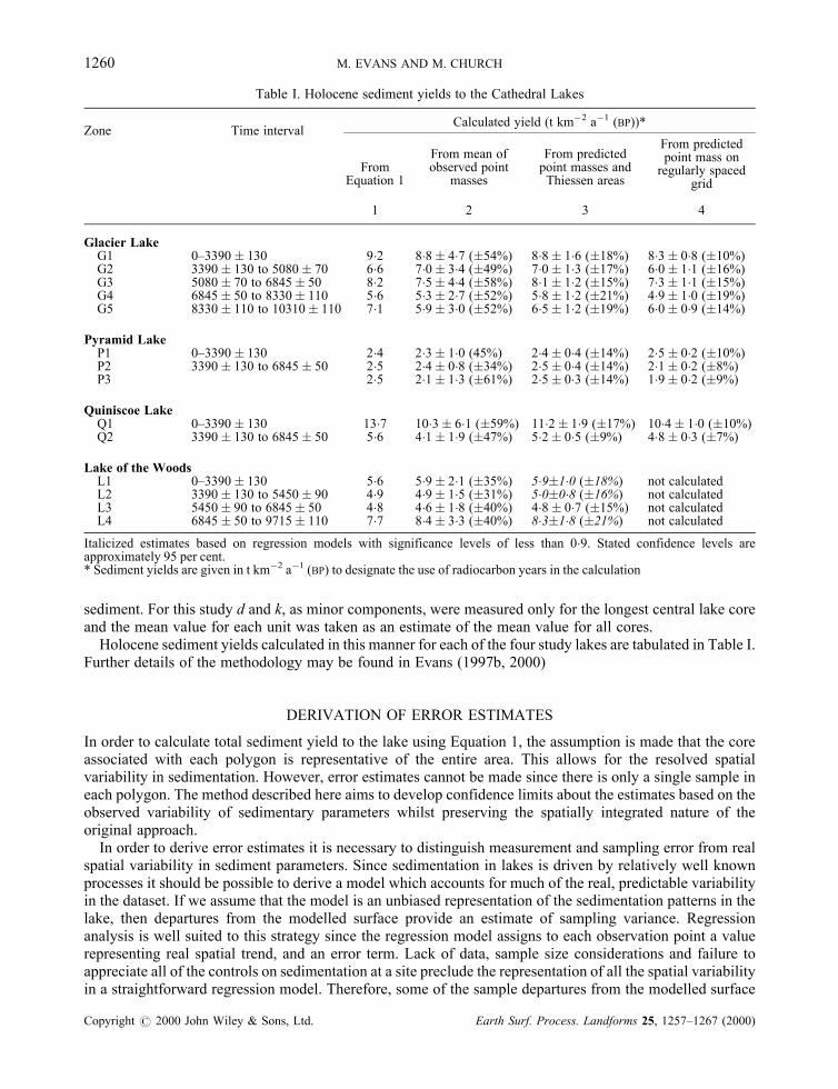
sediment. For this study d and k, as minor components, were measured only for the longest central lake coreand the mean value for each unit was taken as an estimate of the mean value for all cores.Holocene sediment yields calculated in this manner for each of the four study lakes are tabulated in Table I.

Further details of the methodology may be found in Evans (1997b, 2000)

DERIVATION OF ERROR ESTIMATES

In order to calculate total sediment yield to the lake using Equation 1, the assumption is made that the coreassociated with each polygon is representative of the entire area. This allows for the resolved spatialvariability in sedimentation. However, error estimates cannot be made since there is only a single sample ineach polygon. The method described here aims to develop confidence limits about the estimates based on theobserved variability of sedimentary parameters whilst preserving the spatially integrated nature of theoriginal approach.In order to derive error estimates it is necessary to distinguish measurement and sampling error from real

spatial variability in sediment parameters. Since sedimentation in lakes is driven by relatively well knownprocesses it should be possible to derive a model which accounts for much of the real, predictable variabilityin the dataset. If we assume that the model is an unbiased representation of the sedimentation patterns in thelake, then departures from the modelled surface provide an estimate of sampling variance. Regressionanalysis is well suited to this strategy since the regression model assigns to each observation point a valuerepresenting real spatial trend, and an error term. Lack of data, sample size considerations and failure toappreciate all of the controls on sedimentation at a site preclude the representation of all the spatial variabilityin a straightforward regression model. Therefore, some of the sample departures from the modelled surface

Table I. Holocene sediment yields to the Cathedral Lakes

Zone Time intervalCalculated yield (t kmÿ2 aÿ1 (BP))*

FromEquation 1

From mean ofobserved point

masses

From predictedpoint masses andThiessen areas

From predictedpoint mass onregularly spaced

grid

1 2 3 4

Glacier LakeG1 0±3390� 130 9�2 8�8� 4�7 (�54%) 8�8� 1�6 (�18%) 8�3� 0�8 (�10%)G2 3390� 130 to 5080� 70 6�6 7�0� 3�4 (�49%) 7�0� 1�3 (�17%) 6�0� 1�1 (�16%)G3 5080� 70 to 6845� 50 8�2 7�5� 4�4 (�58%) 8�1� 1�2 (�15%) 7�3� 1�1 (�15%)G4 6845� 50 to 8330� 110 5�6 5�3� 2�7 (�52%) 5�8� 1�2 (�21%) 4�9� 1�0 (�19%)G5 8330� 110 to 10310� 110 7�1 5�9� 3�0 (�52%) 6�5� 1�2 (�19%) 6�0� 0�9 (�14%)

Pyramid LakeP1 0±3390� 130 2�4 2�3� 1�0 (45%) 2�4� 0�4 (�14%) 2�5� 0�2 (�10%)P2 3390� 130 to 6845� 50 2�5 2�4� 0�8 (�34%) 2�5� 0�4 (�14%) 2�1� 0�2 (�8%)P3 2�5 2�1� 1�3 (�61%) 2�5� 0�3 (�14%) 1�9� 0�2 (�9%)

Quiniscoe LakeQ1 0±3390� 130 13�7 10�3� 6�1 (�59%) 11�2� 1�9 (�17%) 10�4� 1�0 (�10%)Q2 3390� 130 to 6845� 50 5�6 4�1� 1�9 (�47%) 5�2� 0�5 (�9%) 4�8� 0�3 (�7%)

Lake of the WoodsL1 0±3390� 130 5�6 5�9� 2�1 (�35%) 5�9�1�0 (�18%) not calculatedL2 3390� 130 to 5450� 90 4�9 4�9� 1�5 (�31%) 5�0�0�8 (�16%) not calculatedL3 5450� 90 to 6845� 50 4�8 4�6� 1�8 (�40%) 4�8� 0�7 (�15%) not calculatedL4 6845� 50 to 9715� 110 7�7 8�4� 3�3 (�40%) 8�3�1�8 (�21%) not calculated

Italicized estimates based on regression models with significance levels of less than 0�9. Stated confidence levels areapproximately 95 per cent.* Sediment yields are given in t kmÿ2 aÿ1 (BP) to designate the use of radiocarbon years in the calculation



may in fact represent real variability. Consequently, the departures constitute a conservative estimate ofpotential error. Nevertheless, to the extent that the regression surface takes into account the major sources ofpredictable variability, such estimates are a much closer approximation to real error terms than the measure ofvariability derived from the assumption of equal sedimentation across the lake.Accordingly, regression analysis was employed to identify the spatial variability of sediment parameters

associated with in-lake sedimentary processes. The point mass of sediment (Mi) within a given correlatedstratigraphic unit was defined for each core as:

M � ZD 1ÿ L

100

� �� 1ÿ d � k

100

� �� 2�

with terms as defined for Equation 1. Figure 2 presents the spatial pattern of point masses calculated for eachof the four study lakes. Data are presented for each correlated unit. With the exception of Lake of the Woods,axisymmetric patterns of point mass appear consistently between zones in each lake, raising the possibility ofdefining a physically based model of the sediment surface. Given the location of inlet and outlet points andthe elongate shape of the lakes, the initial core sampling strategy in the Quiniscoe, Glacier and Pyramid lakeswas based on the assumptions that maximum sediment variability would be observed downlake, and thatfurther variability due to sediment focusing could be accounted for by cross-lake transects. The assumedimportance of downlake variability rests on the supposition that sedimentation occurs largely by settling froma moving water column. In fact, presence of clay laminae in many of the lake sediments suggests that wintersettling from a still water column under ice may be an important process of sedimentation in the Cathedrallakes. Therefore, further variability in sediment point mass may be associated with water depth. Theintroduction of water depth as a controlling variate also serves to parameterize edge effects wherebysedimentation is limited near shorelines. Multiple regression was employed to predict sediment point massbased on three parameters: distance downlake from the inlet measured parallel to the centre line (x), distancefrom core site to centre line (y), and water depth (z).We propose that a reasonable sedimentation model employing the variates is:

M � Cc � Czz� Cx ln x� Cy ln y �3�

where Cc is a constant term and Cz is the coefficient of proportion for water depth, in effect the massconcentration per unit water volume associated with sedimentation from a water column of varying depth; Cc

and Cz together represent the terms in a linear model for uniform sedimentation from the water column whichmight reasonably represent sedimentation from a still water column during the cold season. The terms Cx andCy are proportional constants for the effects of distance downlake from the main inlet stream (x) and lateraldisplacement from the centreline (y). Preliminary plotting showed that x and y act somewhat non-linearly.Linearization by logarithmic transformation of distances rather than the more usual transformation of thedependent variable was chosen because of the additional additive terms.An apparently systematic sedimentation feature not covered by the model is a local maximum in

sedimentation near or just beyond mid-lake in all three of the axisymmetric lakes. It is not consistentlyassociated with the deepest water. It may be the consequence of sediment focusing by currents includinggyres set up by the wind. To the extent that this effect exists it is acknowledged that the adopted model doesnot provide a complete description of sedimentation in the lakes.Initially, forward stepwise regression of these parameters on point mass was implemented using the

STATISTICA regression module (STATSOFT, 1994). Products and natural logarithms of the parameterswere also included in the analysis. Regression is an appropriate tool since the independent variables areknown with only minimal measurement error. 1ÿ� limits are defined as:

Yi � t�1ÿ �=2; nÿ p�syi �4�

where Yi is the value of Y estimated from the regression, n is the number of cases, p is number of parameters,


LACUSTRINE SEDIMENT ACCUMULATION 1261

Figure 2. Spatial patterns of pointmass (tmÿ2) plotted for correlation zones in (a)Glacier Lake, (b) PyramidLake, (c)Quiniscoe Lake, (d)Lake of the Woods. For one panel in each lake the appropriate Thiessen grid is shown





1ÿ� is significance level, nÿp are degrees of freedom for Student's t, and Syi is the estimated standarddeviation of Yi.Because of the limited number of cores in each lake, estimation of tight confidence intervals around

predicted values of the dependent variable requires that the number of parameters in the model be minimized.Therefore parameters that could be removed from the initial model without significantly affecting the R2

value or the standard error of the estimate were eliminated. All parameters that were functions of otherparameters in the model were also excluded at this stage. Preference was given to models with no outliersgreater than three standard deviations from the mean. All the models presented below meet this criterion.Normal plots of the residuals were checked to avoid gross violations of the assumption of normallydistributed residuals. This produced statistically significant regression, models (� 0�95) for all of thestratigraphic zones in Glacier and Pyramid lakes. Significant models were also derived for the upper twozones of Quiniscoe Lake (because of difficulty with coring, a full suite of cores spanning the entire HoloceneEpoch was not available from this lake). In Lake of the Woods the models derived had much lower levels ofsignificance. The models are summarized in Table II. Analyses of variance for the models show the generallyhigh proportion of variance covered by the regressions (Lake of the Woods excepted): summary results areincluded in Table II.The final models for Glacier and Pyramid lakes have a common form (M = a� bz ÿclnx) interpretable in

physical terms. The second term indicates sedimentation proportional to water depth, consistent with settlingfrom a mixed water column. It may also relate to focusing of sediment to deeper water. The third termindicates a logarithmic decline in sedimentation with downlake distance which is consistent with materialsettling from a water column in motion downlake. The terms of the regression equation therefore appear tocapture two modes of sedimentation, perhaps relating to the annual cycle of freezing and melting. Theregression model for Quiniscoe Lake is very similar to that discussed for Glacier and Pyramid but y, the cross-lake distance, is substituted for water depth. This pattern is consistent for both zones, and reflects strongfocusing of sediment towards the central long axis of the lake even in areas of relatively shallow water. If theregression model for Quiniscoe is forced to incorporate only z and ln x the correlation is reduced and thestandard error increases by c. 20 per cent for both zones. The most likely reason for the difference between thebasins would appear to be morphology, with Quiniscoe being divided into two basins. However, if theregression is repeated using only the main basin, results very similar to those for the whole lake are produced.An alternative possibility is that high local wind speeds in the Quiniscoe valley exert singular effects on thewater circulation and pattern of sedimentation.

Table II. Regression models of point mass in the Cathedral lakes

Zone n Regression model R2Adjusted

R2 SE df, F p<

G1 12 M = 2�2017� 0�0449 zÿ0�3623 ln x 0�74 0�69 0�18 2,9 13�0 0�0002G2 10 M = 0�8089� 0�0572 zÿ0�1506 ln x 0�89 0�85 0�043 2,7 27�1 0�0005G3 10 M = 1�1616�0�0613 zÿ0�2121 ln x 0�90 0�87 0�055 2,7 30�1 0�0004G4 11 M = 0�4389� 0�0305 zÿ0�0759 ln x 0�63 0�54 0�054 2,8 6�78 0�02G5 11 M = 0�8026� 0�0410 zÿ0�1385 ln x 0�78 0�73 0�063 2,8 14�3 0�002P1 11 M = 0�8159ÿ 0�0113 zÿ0�1196 ln x 0�86 0�84 0�042 2,8 24�7 0�0004P2 11 M = 0�5266� 0�0129 zÿ0�0814 ln x 0�69 0�64 0�052 2,8 8�9 0�009P3 10 M = 0�4564� 0�0185 zÿ0�0835 ln x 0�89 0�84 0�031 2,7 29�8 0�0004Q1 13 M = 5�652� 0�0107 yÿ0�848 ln x 0�93 0�86 0�24 2,10 13�7 0�0002Q2 12 M = 2�037� 0�0042 yÿ0�290 ln x 0�91 0�89 0�056 2,9 14�8 0�0002L1 10 M = 0�0845� 0�000002 x2�0�000015

y2ÿ0�0253z 0�46 0�12 0�037 3,6 1�71 0�262L2 10 M = 0�0788� 0�000005 y2ÿ0�0083 ln x 0�32 0�18 0�020 2,7 1�65 0�259L3 10 M = 0�2116ÿ 0�0209 ln yÿ0�0315 ln

x� 0�0169z 0�69 0�55 0�012 3,6 4�38 0�059L4* 10 M = 0�5020� 0�0533zÿ0�106 ln R 0�49 0�40 0�056 2,7 3�38 0�09* Additional parameter R included in regression model is the direct distance from the inflow to the core site as opposed to thedistance parallel to the central core transect. For L4 this is a better predictor of point mass



The regression equations for Lake of the Woods are weakly significant and vary between zones. It is notclear that physical significance may be ascribed to the models in any straightforward manner. However, thestandard errors for the regressions are acceptably low so that the regression models may be used to modelstructured variability in the lake. The implication is that patterns of sedimentation in Lake of the Woods areconsiderably more complex than in the other lakes. This may be a result of the unusual configuration of thelake, with the outflow located close to the inflow, and of the extreme shallowness of the lake.The regression model allows the estimation of the point mass and confidence limits for the prediction at

any point in the lake. If we accept that the computed models describe the systematic variability in sedimentpoint mass within the lakes, then the confidence limits around the estimated point masses represent thesampling and measurement errors associated with the point mass measure. To facilitate direct comparisonwith the conventional approach (Equation 1), point mass was predicted for the original core locations in thelake. The whole-lake mass (MT) was obtained by summing the products of predicted point mass at the coresite (Mi) and the area (Ai) of the Thiessen polygon around the core, i.e.

MT �X�MiAi� �5�

Confidence limits around the predicted point masses were calculated using matrix methods for multipleregression as described by Neter et al. (1989) and values syi from Equation 4. Confidence limits can beusefully calculated using Mathcad (Mathsoft, 1995) or similar software to perform the matrix operations. The95 per cent confidence limits for the MT are then derived as the square root of the summed squares of theindividual confidence limits. In the summation, the individual limits are weighted by the area of the Thiessenpolygon surrounding the core site, so that the estimated error at each core location contributes to the overallerror estimate in the same proportion as the core site contributes to the total sediment accumulation estimate.Rate of sediment yield (Y) is calculated as:

Y � MT100T

ÿ �t

� ��6�

where t is the time span of the stratigraphic unit in radiocarbon years. The 95 per cent confidence limits of Yare estimated by combining the limits for M, T and t. For the trap efficiency (T) the envelope limits of theBrune curve are assumed to represent 95 per cent confidence limits. For the radiocarbon dates the reportedtwo standard deviation confidence limit was used.The combined error, Ei, can be calculated as: 7

Ei �Xni�1

�Y

�pi

� �2

E2i

" #12

�7�

where Ei is estimated error of parameter pi (see for example Burrough, 1986).The net results of these analyses are sediment yield estimates with approximate 95 per cent confidence

limits which include error from the sediment parameters, dating, and the trap efficiency estimates. Table Ipresents these values (column 3) along with the conventional sediment yield estimates derived by equation 1(column 1). Also given in Table I for comparison are yield and error estimates based on the simple,unweighted mean and standard error of the calculated point masses (column 2). These estimates derive fromthe assumption that there is no structure to the point mass surface and demonstrate the improvement inprecision achieved using the regression technique. However, once the regression models have beenconstructed we may ignore the original sampling points. Integrating the point mass surface across the lakegives the mass of sediment in the stratigraphic zone. Table I (column 4) presents sediment yield estimatesderived by integrating the regression surfaces across the lake area. For each lake, point mass has beenestimated at the intersections of an equally spaced grid across the lake area. Around 100 points have been



calculated for each lake (Quiniscoe 88 points, Pyramid, 92 points, Glacier 146 points). Values for Lake of theWoods have not been calculated because of the weakness of the regression fit for this lake. Yields calculatedin this way are consistently lower than those based simply on the coring location. This may be due, in part, tothe extrapolation of the fitted surface to the shallow edges of the lake in comparison with the extension ofpoint results into shallow water by Thiessen averaging, which may overestimate deposition. The problem ofextrapolation of point sedimentation estimates to shallow water has been raised by Dearing and Foster (1993)who demonstrate significant impacts on the accuracy of sediment accumulation estimates. The Cathedrallakes are steeply shelving. On the basis of direct observation of the lake bed it is estimated that the littoralzone, where sedimentation is limited by wave action, extends only 1±2 m from the shore. For the threeaxisymmetric lakes this ranges from 1�5 to 3�5 per cent of lake area so that the effects on accuracy arerelatively small. Since the edge effects are partially parameterized by the water depth term, the integratedsediment yield estimates are regarded as the most accurate. However, error estimates for the integrated yieldestimates are lower than those for the Thiessen averaged estimate because the non-linear expansion of theerror estimates in the calculation of whole-lake confidence limits yields lower values for larger numbers ofpoints. Consequently the arbitrary selection of grid size for the integration affects the calculated error.Therefore, the most conservative estimates of precision derive from the yield calculation based on regressionestimates of sedimentation at just the original coring sites.

DISCUSSION AND CONCLUSIONS

In most cases there is good agreement between the estimates of sediment yield made by the conventional andregression-based methods. In all cases, with the exception of Q1, the conventional estimate (Equation 1) lieswithin the 95 per cent confidence limits of the regression-based estimates. In all lakes, the regression-basedestimates demonstrate the same pattern of sediment yield as the conventional approach, although themagnitude of late Holocene fluctuations in Glacier Lake is reduced. Some of the variation between the twoestimates stems from the ability to estimate point mass for core sites where it proved logistically impossible torecover full sediment cores. In the initial estimates missing strata were dealt with by expanding the polygonaround the adjacent core. In the regression technique the missing data are estimated from the appropriateregression equation.The significant advantage of the regression technique is the ability to assess the statistical significance of

observed fluctuations in point sediment accumulation by dividing structured spatial variation from anunstructured residual. The latter is a more realistic estimate of sampling error in comparison with estimatesbased on the model of unstructured variance. Maximum potential error in yield estimates based on thestandard error of the mean sedimentation data varied between 31 and 61 per cent of estimated sediment yieldfor Holocene intervals in the four study lakes. In contrast, application of the regression technique producesmaximum potential error estimates ranging from 9 to 21 per cent of estimated yield. These error estimates aresufficiently tight to allow detection of real variability in Holocene sediment yield from the lacustrine records.The development of relatively tight confidence intervals for the yield estimate without the need for extensivereplicate coring significantly reduces the costs of producing well constrained estimates. In addition, themethod limits loss of information stemming from practical difficulties in the field by allowing estimates to bemade for locations where cores could not be recovered.In lakes where the major controls on sedimentation patterns are easily identified on a priori grounds,

allowing the development of models with low standard error values, the method appears to producereasonably tight confidence limits. The best results were achieved in the lakes with simple elongatemorphometry where the form of the regression equation may be assigned physical significance. Morecomplex configuration at Lake of the Woods produced the least improvement in the magnitude of errorestimates. With further testing of the technique in lakes with a range of morphometries it may be possible todevelop guidelines on lake basin configurations where sediment patterns are most predictable andconsequently estimated error is minimized.Dearing and Foster (1993) question the cost effectiveness of multicore studies because of the relatively

high coefficients of variability associated with estimates of mean accumulation rate from 33 cores in Llyn



Geirionydd. However, much of this variability is due to real changes in sedimentation pattern which theynote. It has been shown here that, by accounting for the majority of this variability, the error terms of sedimentyield estimates can be kept acceptably small. The purpose of lake sediment studies is commonly to assess thenature of temporal change in sedimentation. The increased precision of estimation, along with the generationof confidence limits which allow the significance of changes to be assessed, are therefore a strong argumentfor the judicious use of multicore approaches to sediment yield estimation.

ACKNOWLEDGEMENTS

Collection of the data upon which this analysis is based was funded by NSERC grant A7073 to OlavSlaymaker. Reviews from Ian Foster and John Dearing helped us to clarify aspects of the paper.

REFERENCES

Bacon CR. 1981. Eruptive history of Mount Mazama and Crater Lake Caldera, Cascade Range, U.S.A. Journal of Volcanology andGeothermal Research 18: 57±115.

Brune GM. 1953. Trap efficiency of reservoirs. Transactions of the American Geophysical Union 34(3): 407±417.Burrough PA. 1986. Principles of Geographical Information Systems for Land Resources Assessment. Clarendon: Oxford.Dearing JA, and Foster, IDL. 1993. Lake sediments and geomorphological processes: some thoughts. In Geomorphology of Lakes andReservoirs, McManus J, Duck RW (eds). Wiley: Chichester; 5±14.

Evans M. 1997a. Temporal and spatial representativeness of alpine sediment yields: Cascade mountains, British Columbia. EarthSurface Processes and Landforms 22: 287±295.

Evans, M. (1997b) Holocene sediment yield and geomorphic sensitivity in alpine landscapes, Cathedral Lakes, British Columbia. PhDThesis, Department of Geography, University of British Columbia.

Evans, M. (2000) Slope±channel linkages as a control on geomorphic sensitivity in alpine basins, Cascade Mountains, BritishColumbia. In Geomorphology, Human Activity and Global Environmental Change, Slaymaker O (ed.). Wiley: Chichester; 95±115.

Foster IDL, Dearing JA, Grew R, and Orend K. (1990) The sedimentary database. In Erosion, Transport, and Deposition Processes.Walling DE, Yair A, Berkowicz S (eds). IAHS Publication No. 189: 19±43.

Fulton RJ. (1971) Radiocarbon Geochronology of Southern British Columbia. Geological Survey of Canada Paper 71-37.HaÈkanson L, and Jansson, M. (1983) Principles of Lake Sedimentology: Springer-Verlag: Berlin.MathSoft (1995) MathCad 6.0: MathSoft Inc.Neter J, Wasserman W, Kutner M. (1989) Applied Linear Regression Models. Irwin: Homewood, Illinois.O'Hara SL, Street-Perrottt FA, Burt TP. 1993. Accelerated soil erosion around a Mexican highland lake caused by prehispanicagriculture. Nature 362: 48±51.

STATSOFT (1994) STATISTICA for windows, version 4�5. STATSOFT Inc.Sugden DE, Summerfield MA, Burt TP. 1997. Linking short-term geomorphic processes to landscape evolution. Earth SurfaceProcesses and Landforms 22(3): 193±195.



Documents

A method for error analysis of sediment yields derived from estimates of lacustrine sediment accumulation