A Method for Rigorous Development

of Fault-Tolerant Systems

Ilya Lopatkin

A thesis submitted for the degree of Doctor of Philosophy at

Newcastle University

School of Computing Science

Newcastle University

Newcastle upon Tyne, UK

April 2013

Abstract

With the rapid development of information systems and our increasing

dependency on computer-based systems, ensuring their dependability be-

comes one the most important concerns during system development. This

is especially true for the mission and safety critical systems on which we

rely not to put significant resources and lives at risk.

Development of critical systems traditionally involves formal modelling

as a fault prevention mechanism. At the same time, systems typically

support fault tolerance mechanisms to mitigate runtime errors. However,

fault tolerance modelling and, in particular, rigorous definitions of fault

tolerance requirements, fault assumptions and system recovery have not

been given enough attention during formal system development.

The main contribution of this research is in developing a method for

top-down formal design of fault tolerant systems. The refinement-based

method provides modelling guidelines presented in the following form:

• a set of modelling principles for systematic modelling of fault toler-

ance,

• a fault tolerance refinement strategy, and

• a library of generic modelling patterns assisting in disciplined inte-

gration of error detection and error recovery steps into models.

The method supports separation of normal and fault tolerant system be-

haviour during modelling. It provides an environment for explicit mod-

elling of fault tolerance and modal aspects of system behaviour which

ensure rigour of the proposed development process.

The method is supported by tools that are smoothly integrated into an

industry-strength development environment.

The proposed method is demonstrated on two case studies. In particular,

the evaluation is carried out using a medium-scale industrial case study

from the aerospace domain.

The method is shown to provide support for explicit modelling of fault

tolerance, to reduce the development efforts during modelling, to support

reuse of fault tolerance modelling, and to facilitate adoption of formal

methods.

Acknowledgements

I would like to express my gratitude to all those who have provided support

during the years of this work. Firstly, I would like to thank my supervisor

Alexander Romanovsky for his valuable guidance and generous feedback

given throughout the research. I am also thankful to my thesis committee

members John Fitzgerald, Aad van Moorsel, and Cristina Gacek for their

useful and timely advice at different stages of work.

I am grateful to my colleagues at the School of Computing Science at

Newcastle University for their helpful feedback on various aspects of my

research. Special thanks go to Alexei Iliasov for his collaboration and

fruitful discussions, and Anirban Bhattacharyya for his support.

During my studies, I had an opportunity to visit the Department of In-

formation Technologies at the Abo Akademi University, Finland. I would

like to thank Elena Troubitsyna, Yuliya Prokhorova, and Linas Laibinis

for their productive collaboration and hospitality.

I want to thank all colleagues who has been working on the DEPLOY

project. On top of useful collaborations mentioned above, the project

provided extensive research and application material that served as a basis

for my studies.

I am grateful to the DEPLOY project, the TrAmS platform grant, and

the School of Computing Science at Newcastle University for providing

financial support for conducting this research.

Special thanks goes to the thesis examiners Yamine Ait-Ameur and Tom

Anderson for productive discussions and highly valuable feedback on this

work.

Last but not least, I would like to thank my parents and my brother.

This work would not have been done without their encouragement and

support. I am especially grateful to my wife Julia for her understanding

and patience during this long endeavour.

Declaration

I certify that no part of the material offered has been previously submitted by me for

a degree or other qualification in this or any other University.

Published Work

Part of the work presented in this thesis has or will have appeared as follows:

1. The FT/Mode Views method presented in Chapter 3, the airlock case study used

in Chapter 4, and initial ideas of pattern-based development method appeared

in:

I. Lopatkin, A. Iliasov, and A. Romanovsky. On Fault Tolerance

Reuse during Refinement. In: Proceedings of the 2nd Interna-

tional Workshop on Software Engineering for Resilient Systems

(SERENE 2010), ACM, London (UK), April 2010.

The research was carried out by I. Lopatkin with guidance and under supervision

of the co-authors.

2. A first version of the AOCS case study developed using the FT/Mode Views

approach and presented in Chapter 5 was published in:

I. Lopatkin, A. Iliasov, and A. Romanovsky. Rigorous Devel-

opment of Dependable Systems Using Fault Tolerance Views.

In: Proceedings of the 22nd International Symposium on Soft-

ware Reliability Engineering (ISSRE 2011), IEEE, Hiroshima

(Japan), 2011.

The full version of the case study development appeared as a technical report

in:

I. Lopatkin, A. Iliasov, and A. Romanovsky. Rigorous Devel-

opment of Dependable Systems Using Fault Tolerance Views.

School of Computing Science, University of Newcastle upon

Tyne, UK, 2011. School of Computing Science Technical Re-

port Series 1234.

iii

The research was carried out by I. Lopatkin with guidance and under supervision

of the co-authors.

3. Patterns for modelling control systems used as a basis for Section 4.8 were

published in:

I. Lopatkin, A. Iliasov, A. Romanovsky, Y. Prokhorova, and E.

Troubitsyna. Patterns for Representing FMEA in Formal Spec-

ification of Control Systems. In: Proceedings of the 13th IEEE

International Symposium on High-Assurance Systems Engineer-

ing (HASE 2011). IEEE, Boca Raton, Florida, USA, 2011.

The initial patterns were defined by I. Lopatkin and Y. Prokhorova under the su-

pervision of the remaining co-authors. The current work identifies and reserves

a development step for incorporating the FMEA patterns. See more details in

Section 4.8.

4. A summary of the development method presented in the thesis appeared as:

I. Lopatkin, A. Iliasov, and A. Romanovsky. Rigorous Step-

Wise Development of Fault Tolerance. Fast abstract at the

18th IEEE Pacific Rim International Symposium on Dependable

Computing (PRDC 2012). Niigata (Japan), November 2012.

iv

Contents

Declaration iii

Contents v

List of Figures ix

1 Introduction 1

1.1 Motivations . . . . . . . . . . . . . . . . . . . . . . . . . . . . . . . . 1

1.2 Research Hypotheses . . . . . . . . . . . . . . . . . . . . . . . . . . . 2

1.3 Research Methodology and Contributions . . . . . . . . . . . . . . . . 2

1.4 Thesis Structure . . . . . . . . . . . . . . . . . . . . . . . . . . . . . . 3

2 Background 4

2.1 Modelling and Formal Methods . . . . . . . . . . . . . . . . . . . . . 4

2.1.1 Usage of formal methods today . . . . . . . . . . . . . . . . . 4

2.1.2 Success stories and problems . . . . . . . . . . . . . . . . . . . 6

2.1.3 System context . . . . . . . . . . . . . . . . . . . . . . . . . . 7

2.1.4 Event-B . . . . . . . . . . . . . . . . . . . . . . . . . . . . . . 8

2.1.5 Usage of Event-B in industrial and academic settings . . . . . 10

2.2 Fault Tolerance . . . . . . . . . . . . . . . . . . . . . . . . . . . . . . 11

2.2.1 Definitions and taxonomy . . . . . . . . . . . . . . . . . . . . 11

2.2.2 Realistic systems and fault tolerance . . . . . . . . . . . . . . 12

2.2.3 Fault analysis and formal modelling of fault tolerance . . . . . 15

2.3 Views . . . . . . . . . . . . . . . . . . . . . . . . . . . . . . . . . . . 18

2.4 Problem Statement . . . . . . . . . . . . . . . . . . . . . . . . . . . . 20

2.5 Conclusions . . . . . . . . . . . . . . . . . . . . . . . . . . . . . . . . 21

3 Modal and Fault Tolerance Views 22

3.1 Overview and Definitions . . . . . . . . . . . . . . . . . . . . . . . . . 22

3.2 Views Construction . . . . . . . . . . . . . . . . . . . . . . . . . . . . 23

3.3 Views Refinement . . . . . . . . . . . . . . . . . . . . . . . . . . . . . 25

3.3.1 Mode refinement rules . . . . . . . . . . . . . . . . . . . . . . 26

v

3.3.2 Transition refinement rules . . . . . . . . . . . . . . . . . . . . 26

3.4 Formalisation . . . . . . . . . . . . . . . . . . . . . . . . . . . . . . . 27

3.4.1 Well-definedness conditions . . . . . . . . . . . . . . . . . . . 27

3.4.2 Event-B consistency conditions . . . . . . . . . . . . . . . . . 29

3.4.3 Modal views refinement conditions . . . . . . . . . . . . . . . 31

3.5 Conclusions and Limitations . . . . . . . . . . . . . . . . . . . . . . . 32

4 Development Method 34

4.1 Assumptions and Principles . . . . . . . . . . . . . . . . . . . . . . . 35

4.1.1 Multi-view development . . . . . . . . . . . . . . . . . . . . . 36

4.1.2 Co-refinement and restricted modelling . . . . . . . . . . . . . 36

4.1.3 Behaviour restriction . . . . . . . . . . . . . . . . . . . . . . . 37

4.1.4 System environment . . . . . . . . . . . . . . . . . . . . . . . 38

4.1.5 Implementable causality . . . . . . . . . . . . . . . . . . . . . 39

4.1.6 Reactive systems and property coverage . . . . . . . . . . . . 40

4.1.7 Error modelling . . . . . . . . . . . . . . . . . . . . . . . . . . 41

4.1.8 Refinement planning . . . . . . . . . . . . . . . . . . . . . . . 42

4.2 Refinement Strategy . . . . . . . . . . . . . . . . . . . . . . . . . . . 43

4.3 Airlock Case Study . . . . . . . . . . . . . . . . . . . . . . . . . . . . 45

4.4 Abstract System Fault Tolerance Classes . . . . . . . . . . . . . . . . 49

4.4.1 Safe stop pattern . . . . . . . . . . . . . . . . . . . . . . . . . 50

4.4.2 Abstract modal views . . . . . . . . . . . . . . . . . . . . . . . 51

4.4.3 Application in Event-B . . . . . . . . . . . . . . . . . . . . . . 52

4.5 Fault Tolerant Component Refinement . . . . . . . . . . . . . . . . . 55

4.5.1 Error state variable pattern . . . . . . . . . . . . . . . . . . . 55

4.5.2 Error state invariant pattern . . . . . . . . . . . . . . . . . . . 56

4.5.3 Fault tolerant behaviour pattern . . . . . . . . . . . . . . . . . 57

4.5.4 Modal views . . . . . . . . . . . . . . . . . . . . . . . . . . . . 58

4.5.5 Application in Event-B . . . . . . . . . . . . . . . . . . . . . . 60

4.6 Behaviour Restriction . . . . . . . . . . . . . . . . . . . . . . . . . . . 64

4.6.1 Behaviour restriction pattern . . . . . . . . . . . . . . . . . . 64

4.6.2 Modes for functionality and fault tolerance . . . . . . . . . . . 65

4.6.3 Behaviour restriction by modal views . . . . . . . . . . . . . . 65

4.6.4 Application in Event-B . . . . . . . . . . . . . . . . . . . . . . 67

4.7 Hardware . . . . . . . . . . . . . . . . . . . . . . . . . . . . . . . . . 69

4.7.1 Application of fault tolerant component refinement . . . . . . 70

4.7.2 Application in Event-B . . . . . . . . . . . . . . . . . . . . . . 70

4.8 Control Cycle . . . . . . . . . . . . . . . . . . . . . . . . . . . . . . . 71

4.8.1 Control cycle pattern . . . . . . . . . . . . . . . . . . . . . . . 72

4.8.2 Sensing pattern . . . . . . . . . . . . . . . . . . . . . . . . . . 72

vi

4.8.3 Error detection pattern . . . . . . . . . . . . . . . . . . . . . . 73

4.8.4 Control phase patterns . . . . . . . . . . . . . . . . . . . . . . 73

4.8.5 Prediction phase pattern . . . . . . . . . . . . . . . . . . . . . 74

4.8.6 Application in Event-B . . . . . . . . . . . . . . . . . . . . . . 75

4.9 Summary of Patterns . . . . . . . . . . . . . . . . . . . . . . . . . . . 79

4.10 Conclusions . . . . . . . . . . . . . . . . . . . . . . . . . . . . . . . . 80

5 Evaluation 81

5.1 Requirements for AOCS . . . . . . . . . . . . . . . . . . . . . . . . . 82

5.2 AOCS modelling . . . . . . . . . . . . . . . . . . . . . . . . . . . . . 85

5.2.1 Functional model M0 . . . . . . . . . . . . . . . . . . . . . . . 86

5.2.2 Safe stop at M1 . . . . . . . . . . . . . . . . . . . . . . . . . . 87

5.2.3 Functional refinement at M2 . . . . . . . . . . . . . . . . . . . 88

5.2.4 Functional refinement at M3 . . . . . . . . . . . . . . . . . . . 90

5.2.5 Fault tolerant component refinement at M4 . . . . . . . . . . 93

5.2.6 Behaviour restriction at M4 . . . . . . . . . . . . . . . . . . . 95

5.3 Conclusions . . . . . . . . . . . . . . . . . . . . . . . . . . . . . . . . 96

6 Conclusions 98

6.1 Discussions and Directions of Further Research . . . . . . . . . . . . 98

6.2 Summary and Contributions . . . . . . . . . . . . . . . . . . . . . . . 100

References 103

Appendix A: Airlock Case Study Model 117

A.1 Context C0 . . . . . . . . . . . . . . . . . . . . . . . . . . . . . . . . 117

A.2 Machine M0 . . . . . . . . . . . . . . . . . . . . . . . . . . . . . . . . 117

A.3 Machine M1 . . . . . . . . . . . . . . . . . . . . . . . . . . . . . . . . 120

A.4 Context C2 . . . . . . . . . . . . . . . . . . . . . . . . . . . . . . . . 123

A.5 Machine M2 . . . . . . . . . . . . . . . . . . . . . . . . . . . . . . . . 124

A.6 Machine M3 . . . . . . . . . . . . . . . . . . . . . . . . . . . . . . . . 128

A.7 Machine M4 . . . . . . . . . . . . . . . . . . . . . . . . . . . . . . . . 133

A.8 Context C5 . . . . . . . . . . . . . . . . . . . . . . . . . . . . . . . . 144

A.9 Machine M5 . . . . . . . . . . . . . . . . . . . . . . . . . . . . . . . . 144

Appendix B: AOCS Case Study Model 158

B.1 Context C0 . . . . . . . . . . . . . . . . . . . . . . . . . . . . . . . . 158

B.2 Machine M0 . . . . . . . . . . . . . . . . . . . . . . . . . . . . . . . . 158

B.3 Machine M1 . . . . . . . . . . . . . . . . . . . . . . . . . . . . . . . . 160

B.4 Context C2 . . . . . . . . . . . . . . . . . . . . . . . . . . . . . . . . 162

B.5 Machine M2 . . . . . . . . . . . . . . . . . . . . . . . . . . . . . . . . 162

vii

B.6 Machine M3 . . . . . . . . . . . . . . . . . . . . . . . . . . . . . . . . 166

B.7 Machine M4 . . . . . . . . . . . . . . . . . . . . . . . . . . . . . . . . 171

viii

List of Figures

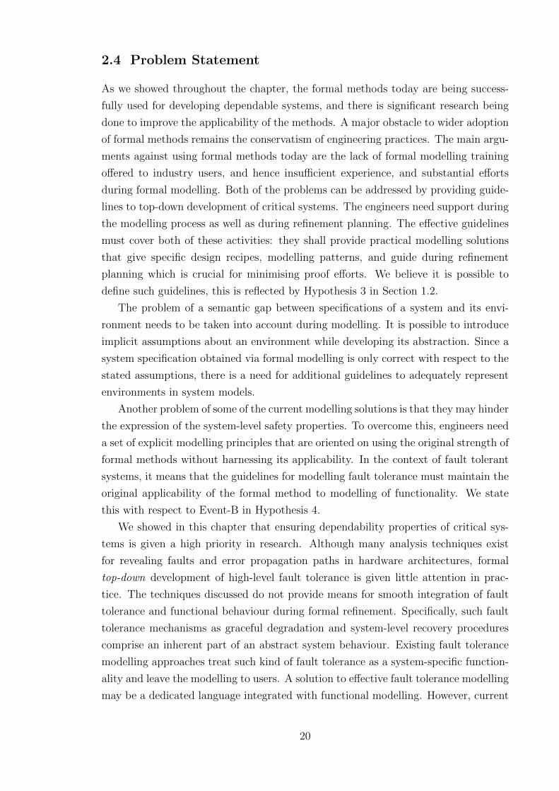
3.1 Example of a modal view . . . . . . . . . . . . . . . . . . . . . . . . . 24

3.2 Modal views development chain . . . . . . . . . . . . . . . . . . . . . 25

3.3 Example of a modal view refinement . . . . . . . . . . . . . . . . . . 26

4.1 Properties and behaviour . . . . . . . . . . . . . . . . . . . . . . . . . 37

4.2 The steps of the method . . . . . . . . . . . . . . . . . . . . . . . . . 43

4.3 The airlock system . . . . . . . . . . . . . . . . . . . . . . . . . . . . 45

4.4 Two abstract classes of fault tolerant systems . . . . . . . . . . . . . 51

4.5 Modal view of a safe stop system . . . . . . . . . . . . . . . . . . . . 52

4.6 Modal view associated with M1 . . . . . . . . . . . . . . . . . . . . . 55

4.7 Error split template . . . . . . . . . . . . . . . . . . . . . . . . . . . . 59

4.8 Behavioural split template . . . . . . . . . . . . . . . . . . . . . . . . 59

4.9 Graceful degradation template . . . . . . . . . . . . . . . . . . . . . . 60

4.10 Modal view of airlock M2 model . . . . . . . . . . . . . . . . . . . . . 63

4.11 Modal view of airlock M3 model . . . . . . . . . . . . . . . . . . . . . 67

5.1 AOCS system modes . . . . . . . . . . . . . . . . . . . . . . . . . . . 83

5.2 AOCS case study models . . . . . . . . . . . . . . . . . . . . . . . . . 85

5.3 Modal view of AOCS M2 model . . . . . . . . . . . . . . . . . . . . . 90

5.4 Modal view of AOCS M3 model . . . . . . . . . . . . . . . . . . . . . 92

ix

Chapter 1. Introduction

This chapter initially describes the motivations behind the thesis and the main topics

related to this work. Research questions and hypothesis that we validate in this thesis

are formulated next. Finally, the research methodology, contributions and the thesis

structure are stated.

1.1 Motivations

Computer-based critical systems dependability

Our society is becoming increasingly dependent on computer-based systems due to

the falling costs and improving capabilities of computers. There is a class of systems

called critical that operate with resources of the highest value. Defects in such sys-

tems, unlike commercial day-to-day products, can have a significant impact on the

environment, assets, and human life. Critical systems have to be dependable [Avi+04],

so that they can be justifiably trusted to provide the required services.

Adoption of formal methods

One of the prominent solutions to ensuring systems dependability by fault prevention

and/or fault removal is the inclusion of formal modelling in the development process.

Even though formal methods are not always used in developing industrial systems,

their use in development of dependable systems is increasing and is proven to be cost-

effective [Woo+09]. Among the main current obstacles to adopting formal methods

by industry are the lack of tools and engineers’ experience in formal development. The

latter can be significantly improved by teaching of examples, development patterns,

and modelling practices.

Modelling fault tolerance

It is well-known that one cannot produce a faultless system functioning in a perfect

fault-free environment [LA90]. This is due to many reasons including changing envi-

ronmental conditions, hardware failures, and inevitable mistakes during development.

In order to achieve sufficient levels of dependability, systems need to mitigate faults

during execution by employing fault tolerance mechanisms. While it is theoretically

1

possible to formally produce a system free of bugs, developers cannot assume system

environment to be fault-free. Deterioration of physical components makes it neces-

sary for systems to tolerate low-level errors, such as sensor and actuator failures, to

provide an acceptable level of dependability.

There are a number of safety analysis techniques for modelling low-level errors

and error propagation paths and analysis of system-level effects. However, there is

limited support for high-level design of fault tolerant systems using formal methods.

Top-down development methods have to support fault tolerance modelling at higher

levels of abstraction, where the overall critical system behaviour inherently contains

error recovery procedures.

1.2 Research Hypotheses

The aim of this research is to validate the following hypotheses:

1. It is feasible to develop systems in which fault tolerance is correctly designed.

2. Design of fault tolerance can be integrated into a formal top-down development

process.

3. It is possible to develop a combination of modelling techniques, refinement

strategies and guidelines that facilitate the development of fault tolerance in

a structured, reusable, and tool-supported way.

4. The refinement-based Event-B method supports formal development of fault

tolerant systems.

1.3 Research Methodology and Contributions

The main approach taken in this research is to propose and evaluate a method for

a top-down rigorous development of fault tolerance in critical systems via formal

modelling of faults and system behaviour. The development method relies on two

major contributions:

• a formally introduced concept of fault tolerance (FT) modelling views, accom-

panied by guidelines for its practical application, and

• a set of principles and practices for modelling fault tolerance in state-based

formal methods.

This work binds the two parts together into a single consistent method for modelling

fault tolerance. The approach is exemplified for the Event-B formal method. Two

case studies are developed to evaluate the method and demonstrate its applicability.

The research methodology relies on the following concepts:

2

• Industrial applications and experience. The method benefits from the analysis

of a number of industrial requirements documents within a range of problem

domains including automotive, aerospace, transportation, and business sectors.

The method is targeting industrial scale application.

• Tool support. The method is tool-supported and integrated into an industry

strength modelling environment. The case studies used in this work for evalua-

tion are developed and proved in the Rodin toolset.

• Conservative extension. Modelling of fault tolerance does not alter the original

top-down development method. The proposed method is built on existing formal

semantics and tools used by industry.

• Top-down development of fault tolerance. The method addresses fault tolerance

at all levels of abstraction and provides a hierarchical approach to modelling.

1.4 Thesis Structure

Chapter 2 contains an overview of the research areas relevant to this work. The

concept of Modal and Fault Tolerance Views is described in Chapter 3 as a self-

contained approach to modelling modal and fault tolerance aspects of systems. The

method for refinement-based formal modelling of fault tolerant systems is proposed in

Chapter 4. The method consists of a number of refinement-based modelling solutions

which are used according to a refinement strategy, and a practical application of modal

views. The method is evaluated in Chapter 5 by modelling a second case study from

the aerospace domain. We draw conclusions and discuss limitations of the method in

Chapter 6.

3

Chapter 2. Background

This chapter provides a thesis background and a current state of the art in relevant

research areas. This thesis contributes to the three areas each described in its section:

an overview of the relevant aspects of formal methods is given in Section 2.1, fault

tolerance is addressed in Section 2.2, and the current state of research in multi-views

development is discussed in Section 2.3. We identify the key problems that we intend

to address by this study in Section 2.4 and we draw our conclusions in Section 2.5.

2.1 Modelling and Formal Methods

Modelling is a process of creating an abstraction of (some aspect of) a system with

the purpose of gaining confidence and deeper understanding of the resulting be-

haviour of the system. Different modelling frameworks provide different means of

such assurance. A number of XML-based frameworks such as UML [JBR99; Amb04]

and AADL [AADL] today are widely used by industry engineers to represent the

domain knowledge and system architecture. Known as model-driven engineering

(MDE) [Amb04], such an approach increases the quality of the end products and

the predictability of their behaviour which generally improves systems dependability.

Although there are works on extending semantics and using external analysis tools

for model validation [RSH11; HLV11], the original frameworks do not provide formal

development facilities.

2.1.1 Usage of formal methods today

Formal methods provide high level of assurance by applying mathematical rigour

during the modelling process. Various formal techniques are used at all stages of

system development including requirements engineering [Eas+98; CDV98; Ham+95],

software specification [BS03; Abr96; Abr10; WD96; Jon90], high-level architectural

design [All97; AADL], software design [Jon90; Bac80], implementation [Ros95], and

testing [HBH08]. The thesis focuses on using formal methods at the early phases of

specification and design.

The purpose of a formal specification of the system is to arrive at a correct model

shown to satisfy the requirements. The formal specification is then used at later

4

stages of development to ensure the correctness of the implemented system. Formal

specification may be also used for certification or to validate the correctness of an

already deployed system post factum. There are several types of formal approaches

which differ in their ways of assuring the model correctness.

Model checkers [Cla08] ensure the correctness of a model by executing the be-

havioural part of the models and checking, at each state or a group of states, whether

the required properties hold. Model checkers typically accept properties expressed in

a temporal logic. This allows developers to check liveness properties of the models.

Although various optimisations have provided major improvements in model checking

capabilities, the approach lacks of scalability due to state space explosion on real-world

problems [Pel09].

Another formal approach used in software engineering is test case generation

[Bro+05]. It consists in comparison of the formal specification of a system and its ex-

ecutable implementation. The specification is used to derive test cases which are run

against the implemented code. Thus, the implementation is guaranteed to conform to

the specification with respect to the test case coverage. The derivation of test cases

is typically automated, and the process of implementation can follow the test-driven

development approach [Bec03].

Other approaches closely related to test case generation are assertions and design

by contract. The assertions [Ros95] are properties expressed on the local state of

the programming unit checked statically or at run-time. Some assertions are state-

ments over factual parameters of methods. They represent assumptions about the

parameters passed by another block of code. The assertions can be statically anal-

ysed (proven) given that the guarantees of the caller are also defined. Such pre-

and post-conditions are used during design by contract. There are a number of li-

braries and programming languages supporting the design-by-contract approach such

as: MS Code Contracts [MSCC], MS Spec# library [MSSP], Eiffel programming lan-

guage [Int06], and Java Modelling Language [Cha+06]. In these languages, a formal

specification of the system behaviour is essentially intertwined with the implementa-

tion and is expressed at the same level of abstraction. The mentioned libraries are

language-specific, and are used in practice for finding common programming bugs.

Theorem proving is a rigorous approach to formal assurance of the intended system

behaviour. In proof-based methods [Abr96; Abr10; WD96; Jon90], one specifies the

behaviour of the system and a set of safety properties. A developer is responsible for

showing that the model satisfies the properties by proving proof obligations generated

by the methods. Thus, when the system is implemented according to the specification,

it will maintain the properties during execution. No actual execution of the model is

performed during the formal development. Automatic theorem provers [RV01] may

be also used to prove (a part of) the generated proof obligations. By proving the

5

obligations one guarantees the full coverage of the model state space against the

safety properties specified [WD96; Abr96]. Typically, liveness properties can also be

verified using an external model checker that supports the notation of the method

being used [LB08].

2.1.2 Success stories and problems

A number of surveys [Woo+09; HB95; BH06] report on an industrial uptake of formal

methods during the last 20 years with an increasing use at early phases of specification

and design. The surveys show a generally positive effect of using formal methods on

time and cost of development, and quality of the final product.

Although formal methods are not widely used for developing day-to-day commer-

cial software, the necessity of their use for building highly dependable systems is

evident [Rus89; HG93; HBV10; HB99]. There are a number of successful industrial

projects where formal methods were applied and the resulting systems are now in

operation. In transportation sector, Siemens Transportation Systems [STS](formerly

Matra Transport) heavily uses B as a high-level design language for specification

and proving correctness of the control logic of train systems. Line 14 of the Paris

underground metro [Beh+99] and a train shuttle for Roissy Charles de Gaulle air-

port [BA05] were developed using the company’s established development process

based on B. Notably, both systems are driverless. The B and Event-B methods have

been also used for the development of train signalling systems in Brazil conducted by

the AeS Group [RL12; D15.5].

In microchip design, validation plays a crucial role due to sheer complexity of

microprocessors. Verification and theorem proving have been the major techniques in

validating the instruction set specifications [PJB99; Mur+08; Hun89; Win94]. One

example of a successful application of formal methods is a formal validation of the

instruction set architecture of the XMOS XCore using Event-B [Yua+11].

Some other examples of applications of formal methods include the design and

verification of embedded medical devices [GO11; QNX], subsystems of satellites in

the aerospace domain [Ili+10], voting algorithms [Bry11], and distributed systems

coordination [ASAA09].

The increasing complexity of critical systems make them an appropriate target

for a top-down development approach. The success of applying refinement-based for-

mal methods mainly comes from the ability to design a system incrementally starting

from an abstract representation. By defining an abstraction, the top-down methods

allow developers to capture the essential functions of the system without spreading

the modeller’s attention on details. At each step, the model is formally refined thus

introducing lower-level concepts and behaviour. However, refinement is also an en-

gineering process where design mistakes are inevitable. The process of arriving at

6

a detailed model of a system can be described as a traversal of a tree of models.

A modeller starts from the root, and by refining the initial model he/she traverses

through the tree until he finds an acceptable detailed model. At some point while

verifying the required properties, a modeller can realise that he has made a mistake or

some abstract formal elements prevent from modelling the desired system behaviour.

Then, he needs to rollback and make a change to an abstract model. This leads to

changes in the rest of the already modelled refinements. Therefore, the modelling and

proof efforts for redevelopment of abstract behaviour is generally higher than that of

concrete models due to proofs associated with refinement. To minimise such costs,

there is a need for an effective way to cut out those models and modelling decisions

which are known to be unacceptable a priori.

Despite the success stories and increasing use of formal methods, they are not yet

the rule for developing dependable systems. Among the main problems of adopting

formal methods are a steep learning curve for engineers and a general lack of tool

support [Woo+09]. An effective solution to the former can be a set of principles,

practices, and patterns that teach engineers the right ways to model certain aspects

of the systems within a particular domain or formal method. In object-oriented

software engineering, such approach is now widely used and is known as design pat-

terns [Gam+94].

2.1.3 System context

A formal method is a flexible tool for specifying what a system should do omitting

the details of how it should be done. However, the specification of what a system

must do is a complex task in itself due to a significant semantic gap between informal

language of requirements and a formal language of specification.

The purpose of any artificial system is to bring about changes to its problem

domain. The part of the problem domain that can be observed and changed by a

system represents the system environment, or its context. It can include a part of the

physical world or another technical system or both.

The idea of the system context and analysis of its phenomena is given attention

in the Problem Frames requirements analysis approach [Jac01]. In Problem Frames,

after defining the context of the system, one gradually decomposes both the system

and the environment until a sufficient level of requirements granularity is achieved.

The HJJ approach [HJJ03] builds on the Problem Frames thinking and focuses

on the interface between a control system and its environment. It shows that speci-

fications of many systems may be derived from those which include the context and

its physical phenomena. The process of defining system requirements and its context

provides insights into its intended behaviour, and helps in identifying requirement

ambiguities and inconsistencies [D1.1].

7

Even at the finest level of details, requirements are still informal and have to be

formalised for a concrete specification language. One solution to requirements for-

malisation can be a user-defined explicit mapping of requirement terms into formal

specification terms [JHL11]. Thus, formal reasoning may reveal mistakes and omis-

sions in requirements during modelling. With such a solution, the separation of the

system from its context remains informal.

Different formal methods may provide different means for modelling environments.

The common issue here is a semantic gap between the language used to express an

environment and the formal language for specifying a system behaviour. For example,

a physical environment of a control system may have continuous-time nature that is

expressed using differential equations, and the high-level logic of the system may

require discrete-time modelling. A number of solutions can be used to bridge this

semantic gap: the system model and the environment model may be expressed using

different languages and used during co-simulation [Fit+10], or an abstraction of the

environment can be defined in the target formal language used to specify the system

behaviour [HH11]. In both approaches, the system model has to contain definitions

representing the relevant part of the system context.

2.1.4 Event-B

The development method described in this thesis is exemplified on Event-B formal

method [Abr10]. Event-B is a state-based formalism closely related to Classical

B [Abr96] and Action Systems [BS89]. The step-wise refinement approach is the

corner stone of the Event-B development method. A combination of model elabo-

ration, atomicity refinement and data refinement helps to formally transition from

high-level architectural models to detailed, executable specifications ready for code

generation [EB].

An extensive tool support makes Event-B especially attractive. An integrated

Eclipse-based development environment [ROD] is under active development now and

is well-supported. It is open for extension using the Eclipse plug-in mechanism [ECL].

The main verification technique is theorem proving and the development is sup-

ported by a collection of theorem provers [ATB] while there is also a capable model

checker [PROB].

An Event-B model is defined by a tuple (c, s, P, v, I, RI , E) where c and s are

constants and sets known in the model; v is a vector of model variables; P (c, s) is a

collection of axioms constraining c and s; I is a model invariant limiting the possible

states of v: I(c, s, v). The combination of P and I should characterise a non-empty

collection of suitable constants, sets and model states: ∃c, s, v ·P (c, s)∧I(c, s, v). The

purpose of an invariant is to express model safety properties. In Event-B an invariant

is also used to deduce model variable types.

8

RI is an initialisation action computing initial values for the model variables; it is

typically given in the form of a predicate constraining next values of model variables

without, however, referring to previous values - RI(c, s, v′).

E is a set of model events. The general form of an event in Event-B notation is

name = any p where H(c, s, p, v) then S(c, s, p, v, v′) end

where p is a vector of event parameters, H(c, s, p, v) is an event guard, and

S(c, s, p, v, v′) is an event action expressed as a before-after predicate. An event may

fire as soon as the condition of its guard is satisfied and no other event executes at

the same time. In case there is more than one enabled event at a certain state, the

demonic choice semantics is applied. The result of an event execution is some new

model state v′.

The semantics of an Event-B model is usually given in the form of proof semantics,

based on Dijkstra’s work on weakest precondition. A collection of proof obligations

is generated from the definition of the model and these must be discharged in order

to demonstrate that the model is correct. For an abstract model (a model that is not

a refinement of another model) two such proof obligations are the invariant satisfac-

tion and event feasibility. A new state produced by an event must satisfy the model

invariant:

I(c, s, v) ∧ P (c, s) ∧H(c, s, p, v) ∧ S(c, s, p, v, v′)⇒ I(c, s, v′)

An event must also be feasible, in a sense that an appropriate new state v′ must

exist for some given current state v:

I(c, s, v) ∧ P (c, s) ∧H(c, s, p, v)⇒ ∃v′ · S(c, s, p, v, v′)

There are also proof obligations to establish deadlock freeness, enabledness condi-

tions and a collection of proof obligations for demonstrating Event-B forward simu-

lation refinement [MAV05].

The traces of Event-B machine M are defined as follows. Let us denote the uni-

verse of machine states as Ω. Then Ω is the set of all safe states of a machine:

Ω = v | I(v). For each machine event e ∈ E consider a relational interpretation

[e]R ⊆ Ω× Ω:

[e]R = v 7→ v′ | ∃p · (H(v, p) ∧ S(v, p, v′))

where H, S and p are, respectively, the guard, the body and parameters of event

e. There are two special cases of relational interpretations. The relational form of

initialisation is [INIT]R = id(init) where init ⊆ Ω is the set of initial states for

a machine. The relational form of skip (a stuttering step event of a machine) is

9

[skip]R = id(Ω).

Now, consider set Q of finite sequences of event identifiers, Q = P(seq(E)). Us-

ing relational forms of events, one can convert a sequence q ∈ Q into a relation

ψ(q) ⊆ Ω × Ω. Let 〈〉, 〈e〉 and q a t denote, correspondingly, an empty sequence,

a sequence containing event e and a sequence concatenation of q and t; ψ(q) can be

then obtained using the following procedure:

ψ(〈e〉) = [e]R

ψ(q a t) = ψ(q);ψ(t), q 6= ∅ ∧ t 6= ∅

where ; is the relations composition operator: (f ; g)(x) = g(f(x)). Let us consider

now the sequences contained in set Q. Some of them initiate with an event other

than initialisation, and we need to reject such sequences. Also, some sequences may

represent an empty relation, an event ordering that cannot be realised due to restric-

tions expressed in event guards. We define the traces of machine M as those event

sequences that start with initialisation and represent non-empty relations:

TR(M) = q | q ∈ Q ∧ ∃t · t ∈ Q ∧ q = 〈INIT〉 a t ∧ ψ(q) 6= ∅

2.1.5 Usage of Event-B in industrial and academic settings

This thesis is mainly based on results of the FP7 DEPLOY research project [DEP].

The overall aim of the project is to improve the development process for dependable

systems by using formal methods. One of the project outcomes relevant to this study

is a number of pilot developments modelled by four industrial partners [D1.1; D2.1;

D3.1; D4.1]. During the pilot developments, Event-B has been used for achieving high

system dependability by applying it in a number of different ways: it has been used

as a development method with heavy use of functional refinement, as a specification

language, and as a requirements engineering tool. Based on that experience, this

work focuses on improving the usage of Event-B as a refinement-based specification

language.

Event-B has a flexible notation which allows developers to express and refine sys-

tem behaviour in various ways. Researchers and industrial practitioners have proposed

a number of approaches to modelling in Event-B depending on the goal of modelling

and the target domain. The original approach in J.-R. Abrial’s models [Abr10] mostly

follows a top-down development of reactive systems, and heavily uses data refinement.

Another refinement technique that is given attention mainly in industry is atom-

icity refinement. In atomicity refinement [FBR12], the abstract event is refined by a

group of concrete events. While all the concrete events represent the abstract state

transition, only one concrete event formally refines the abstract event. The group of

events thus represents a series of transitions which refines the abstract atomic action,

10

hence the name. At the concrete level the system becomes sequentially decomposed

which limits the expression of system-level safety properties. The sequential decom-

position of the model has a major influence on further refinements which is discussed

in Chapter 4.

The problem of the semantic gap between the formal expressions of the system and

its context (see Section 2.1.3) also impacts the modelling practices in Event-B. The

properties that the modellers are typically interested in declare relationships between

the system and its environment. Thus, the event guards have to reference system vari-

ables in order to re-establish the invariants. If an event represents the environment,

such a reference in its guards would mean that the environment is aware of the system

state. This is used in [SB11] to model the “tick” event which represents the flow of

time. The event ensures that the system properties hold before advancing the time.

In [But12] the same situation holds for events that represent the environment. The

events representing the physical context refer to the controller state in their guards.

This ensures that the environment changes its state only when the controller has fin-

ished the current control cycle. Such techniques should only be used under explicitly

stated assumptions about the environment and the implementation context. Other-

wise, they may implicitly introduce such assumptions through modelling the system

behaviour. In particular, fault assumptions are essential for specifying system fault

tolerant behaviour which is discussed in the next section.

2.2 Fault Tolerance

Critical systems’ complexity grows along with the societal demand for such systems.

Many systems operate on resources of highest value such as health, lives, time, and

money. We rely on critical systems and thus require developers to apply appropriate

development techniques to ensure safety and efficiency [Kni02]. This essentially means

minimisation of faults contained in the final system.

2.2.1 Definitions and taxonomy

In this work, we follow the terminology and taxonomy of dependable computing

[Avi+04]. Fault is an internal flaw (or an external cause) of a system which re-

sides dormant until certain circumstances arise. When the fault becomes active, it

causes an error, a runtime deviation from a correct system state. An error which

reaches the external interface of the system is considered as a failure of the system

to provide its service. The concepts of error and failure are relative to the hierarchy

under consideration: a failure of an internal component of a system can be considered

as an error within the system.

There are a number of techniques to enhance the system dependability. Fault

11

prevention and fault removal techniques reduce the amount of faults in the product

through enhancing the development process. Rigorous specifications, formal methods,

software verification and testing all target the goal of producing an ideal system that

does not fail.

However, any computer-based system also contains an interface with the physi-

cal world. That interface cannot be ideal due to physical deterioration. Even under

the assumption of running a fault-free software (and especially without such assump-

tion), any system eventually suffers from malfunctioning hardware or unforeseen cir-

cumstances. More generally, any non-deterministic part of the system context may

introduce errors which are out of the system control, such as: physical environment,

human operator mistakes, operating system exceptions, behaviour of the off-the-shelf

components. To mitigate such situations at runtime, developers must introduce re-

dundancy into the system, and fault tolerance [LA90].

Fault tolerance is a term for system mechanisms that are introduced during devel-

opment and are used by the system during runtime to avoid system failure in presence

of faults. Under certain conditions the system cannot provide a full service, and fault

tolerance mechanisms can be used to gracefully degrade system functionality. Fault

tolerance generally includes three phases:

• Error detection. The system must be able to detect that its state or the be-

haviour of its components is abnormal.

• Error recovery (or compensation). When the deviation of the behaviour is

detected, the system performs some action to return to its normal operation.

• Fault treatment. To avoid repetition of the same error, the system can treat the

fault if the cause is found.

The fault tolerance phases and their relationship with the concepts of faults, errors,

and failures are described in [Avi+04].

2.2.2 Realistic systems and fault tolerance

The ultimate purpose of any system is to perform its function. As the complex-

ity increases and additional constraints are enforced by requirements, non-functional

properties become as important as the functional ones. In critical systems, safety

and other dependability properties are major concerns. To improve dependability,

the context of a system has to become wider and include physical phenomena, hard-

ware and other component failures, operator behaviour etc. Any critical system has

to specifically deal with undesired situations to perform its desired function. The

undesired situations constitute an abnormal part of the system behaviour. However,

the concept of “normality” is vague and specific to the system. The border between

12

normal and abnormal behaviour is important, however, it is not always feasible to

fully differentiate between the two. For example, a degraded behaviour of a system is

functional but the actual process of degradation is a reaction to abnormal situations

which is a kind of fault tolerance.

Realistic critical systems may contain up to 35-40% of requirements devoted to

fault tolerance. This is supported by our study of the requirements descriptions pro-

duced by deployment partners for the pilot and mini-pilot studies in the DEPLOY

project. The detailed requirements documents for the case studies are largely con-

fidential, but descriptions of the pilots are provided in public deliverables for the

deployment workpackages [D1.1; D2.1; D3.1; D4.1]. Our study of the requirement

documents shows that the major source of faults considered in these systems is the

environment, including sensors, external networks and human operators. Dealing

with software design faults is never stated as a requirement, and only rarely do re-

quirements define hardware faults (e.g. node crashes in a distributed application) and

state how these need to be addressed.

System requirements normally include description of degraded functionality, the

most typical example being system safe stop. More generally, we observe that the re-

quirements predominantly include information about how general system behaviour

is affected by various abnormal situations. Unfortunately, this information is rarely

explicitly stated as a priority requirement (sometimes, we needed to deduce this in-

formation from other requirements).

It has been found that many system requirements use the concept of operational

modes [Dot+09; IRD09] to refer to different operational conditions resulting in differ-

ent functionalities provided by the system. We observe that the description of system

modes and mode transitions is often intertwined with error recovery. For example, at

the system level, modes may represent fault handling through system degradation.

A final observation is that requirements related to error recovery are often not

structured in a way that makes it easy for modellers to work with these issues. The

relevant requirements are typically scattered over the whole requirements document

and refer to issues related to different levels of abstraction. For example, none of the

documents reviewed had a table of fault assumptions.

Dependability of critical systems is indeed a primary concern and significant efforts

are being spent on analysis and improvement of reliability and safety. Nevertheless,

such systems do fail and their failures often lead to major losses. There are several

well-known examples of critical systems’ failures such as: the Ariane 5 launch fail-

ure [Age96], the losses of the Mars Polar Lander [Lab10] and of the Mars Climate

Orbiter [AA99], and the US and Canada Northeast blackout 2003 [For04]. It is not al-

ways possible to identify a single cause of failure in such cases, it typically represents a

combination of engineering and management omissions. For example, it is well-known

13

that the initial cause of the Ariane 5 failure was a software bug: one of the software

components, the Inertial Reference System (IRS), produced an exception which led

to termination of an important piece of control software. However, the IRS software

was reused from Ariane 4 for which it was tested to work correctly. The impact of

the change of both physical and software environment on the operation of IRS was

not checked rigorously in the new system. This is a clear example of poor reasoning

about environment assumptions. The final trigger for the failure was the error recov-

ery action that shut down both the main IRS component and its duplicate due to

exceptions. The primary cause of such an omission was an incomplete definition of

fault assumptions: the error recovery procedures focused mainly on hardware failures,

and the IRS component was treated as a piece of hardware. The implicit assump-

tion in this case was that the IRS control software always produces correct output,

and hot-swapping is a sufficient recovery action. Absence of design faults in software

which is developed using traditional methods is an unrealistic fault assumption. The

fault tolerance mechanism based on such an invalid assumption led to propagation of

the error and eventually to a system failure.

Various fault tolerance techniques are used nowadays in highly dependable systems

at all levels of operation. In hardware, many techniques are based on hardware

redundancy for fault masking. That is, critical subsystems are built using a number

of spare components and a voting mechanism that together provide a single function.

The well-known example is a Triple Modular Redundancy (TMR) [LV62] which is

built from three replicated active components and ensures fault masking by a voter.

A more general design is called N-modular redundancy (NMR) which can tolerate

(N−1)/2 module faults during the majority voting. These approaches are considered

as static redundancy; no action is performed upon detecting an error as the error is

masked before reaching any other component. A complementary class of techniques

includes dynamic hardware redundancy. These are used primarily in applications that

can operate while receiving temporary erroneous results from hardware components.

For example, duplication with comparison is an error detection mechanism; it uses two

identical modules and a comparison mechanism. It always produces an output from

one of the modules, be it correct or not, and a result of comparing the outputs of the

two modules. The comparison result is then used by a higher-level logic for further

recovery. There are also techniques that involve local reconfiguration of a component

such as hot standby sparing, cold standby sparing, and pair-and-a-spare. With dynamic

redundancy approaches, the reconfiguration process usually takes some time during

which the component is not available or produces erroneous output. These static

and dynamic redundancy techniques are often composed to achieve certain levels of

reliability cost-effectively.

The primary causes of hardware faults are physical deterioration and external

14

interference, whereas the primary faults in software are design faults due to design

complexity [Kni12]. In software, fault tolerance is present to some degree in every

application written using a modern programming language. Exception handling and

the principle of defensive programming form a common practice today. Nevertheless,

it is not sufficient in many safety- and mission-critical applications. A well-known

technique of N-version programming (NVP) is used in complex and/or critical appli-

cations to tackle design faults. In NVP, a number of different teams of developers are

given the same specification to implement their “version” of software [Avi85]. All of

these versions are then deployed in a single component of the system in a way similar

to hardware modules. That is, they run simultaneously and vote on the output (NVP)

or active sparing techniques could be used (recovery blocks). Most often, software is

built using existing libraries, so called off-the-shelf components (COTS). Additional

measures are typically used to ensure the overall dependability of the critical software

when using COTS. COTS wrappers [Pop+01] is the most popular fault tolerance

technique that is given significant attention in research. In the distributed computing

area, which includes business applications and high-throughput computing, there are

solutions for tolerating byzantine faults.

Software fault tolerance has been traditionally an iterative engineering process.

It is usually developed using the same principles as is the software performing the

main functionality of systems. This means that it is susceptible to the same types of

mistakes and, therefore, may contain faults. There is a need for methods and tools for

development of highly dependable systems that would facilitate rigorous development

of fault tolerance and help identify and eliminate faults during design.

2.2.3 Fault analysis and formal modelling of fault tolerance

To adequately handle the abnormal situations and improve dependability properties of

a system, possible faults and failures must be specified and taken into account during

design. There are a number of fault analysis techniques that are used by engineers in

industry to achieve this.

Failure Modes and Effect Analysis (FMEA) is an inductive technique for safety

analysis [FMIC; FMTR; Sto96]. It is a development procedure for analysis of potential

failure modes of a system by listing their severity, probabilities, and effects. Failure

mode is a general term for capturing possible faults, errors, and system failures. The

technique is informal, it represents a part of the development process which helps

engineers organise their expectations of the system failure modes and effects based on

their previous experience. The technique mainly targets failure modes of individual

components and their impact on the system behaviour.

Fault Tree Analysis (FTA) is another technique used in safety and reliability en-

gineering [Ves81]. It is a deductive top down method in which a system failure or

15

another abnormal state is analysed into its low-level causes by using boolean logic.

Given the probabilities of low-level errors (e.g. component failures), the likelihood

of a target system failure can be estimated. Fault trees are used at various stages

of development process from design to maintenance. The process of creating a fault

tree is also informal and is based on engineer’s experience in a specific domain. FTA

targets system and component failures at higher levels and allows for analysis into

lower-level component errors.

In both FMEA and FTA it is an engineer who informally chooses which system fail-

ures need to be analysed. Such information can be also synthesised from the domain

knowledge and a model of how system components are interrelated and communicate

with the system context [McK+05; LGP11]. Hierarchically Performed Hazard Ori-

gin and Propagation Studies (HiPHOPS) [Pap+11] is an example of a model-based

method for semi-automatic safety and reliability analysis. It allows developers to gen-

erate fault trees and FMEA tables based on a model of system architecture expressed

in terms of components and material and data transfers. Such models provide useful

information for the identification of error propagation paths that lead to system fail-

ures, and play an important role in the system design process. Cecilia OCAS [Bie+04]

is another example of a model-based safety assessment framework that is capable of

generating FMEA tables and fault trees from an architectural model. It is based on

the AltaRica [Alt] language and is being used at an industrial level for architectural

safety assessment of avionics systems.

Safety and reliability analysis is necessary for making design decisions during sys-

tem development. As a part of specification, design, and possibly implementation,

formal model of a system typically represents the decisions which were made based

on safety and reliability analysis. Both during fault analysis and formal modelling,

fault assumptions play the key role in defining the resulting behaviour and system

properties [LA90; HJJ03]. A system is designed to perform its function within a

certain environment. Thus, the estimation of the system dependability relies on the

understanding of the environment and assumptions about uncontrolled phenomena.

Wrong assumptions can lead to malfunctioning and unsafe systems which are still

formally correct. Therefore, it is crucial to explicitly define fault assumptions upon

which fault tolerance is modelled and then implemented in the system.

There are a number of studies on formal modelling of fault tolerance. Some re-

search is done on extending original semantics of formal methods with additional fault

tolerance modelling constructs. An example of such an approach is an extension of the

Lustre data flow language for modelling faults and error propagation paths [JH07].

The extended LustreFM language allows developers to specify possible faults of a

component and different aspects of fault activation such as triggers, durations, con-

ditional activations, and error propagation rules. The authors envision the process of

16

safety analysis by using libraries of domain-specific fault model components that can

be specialised for a particular system fault model. A similar approach to specifying

error causality on top of functional models is taken in works on FPTN[FM92] and

FSAP/NuSMV-SA[BV07]. A notable work on extending normal system behaviour

with fault tolerance is described in [Jef+09]. Authors introduce a notion of partial

refinement defined for state machines and use it to formally connect the normal be-

haviour of a system with the fault tolerant one.

There are numerous works on extending process-based formal methods such as

CSP with additional formal constructs for modelling fault tolerant behaviour. One

example could be the Peleska’s method for verification of fault tolerant systems with

CSP [Pel91]. It provides algebraic and assertional techniques and is used in parallel

with top-down design of FT systems. Other studies on extending CSP with FT-

oriented semantics include an improved failures model [BR85] and message recovery

techniques for CSP [Jal89].

Another class of FT modelling techniques include patterns and modelling styles

for modelling fault tolerance in specific formalisms without extending their semantics.

An example of such an approach is [LT04b] which provides a guidance to modelling

fault tolerant control system in B. The authors focus on failsafe systems which can be

safely stopped at any moment of time. The approach starts with an abstract general

specification which is applicable to any failsafe control system. During refinement,

system components are introduced and their failures are associated with the abstract

safe stop. Error detection is paid significant attention as this is the phase where actual

difference between normal and abnormal states is defined. The approach follows a

typical control system design by modelling a control cycle consisting of the sensing,

control, and acting phases. During sensing, errors can be detected and are classified

into recoverable and non-recoverable types. In case when an error leads to a failure,

the control operation is skipped and the system is stopped. A recoverable error is

masked by one of the redundancy techniques, and the control operation continues.

Thus, the functionality of the system is always provided under the assumption of

fault-free components. The assumptions used in the approach limit its applicability.

The approach is adequate for modelling low-level component failures that may be

masked, but it is not designed for specification of graceful degradation and system-

level recovery procedures.

A pattern for modelling fault tolerance in B is proposed in [LT04a]. The paper

introduces a general formal specification pattern to be applied in development of de-

pendable systems with a layered architecture. The pattern adds exception handling

mechanism to each system layer and organizes communication between components

within a hierarchical structure by means of exceptions. The layered exception hierar-

chy pattern is based on top-down refinement. The pattern follows the idea of idealised

17

fault tolerant component (IFTC) introduced in [LA90]. The IFTC is a generic com-

ponent which explicitly differentiates between its normal and abnormal operation,

and specifies the conditions under which it switches between the two. The system is

thus constructed as hierarchical layers of IFTCs. Each component can handle certain

exceptions, and it propagates the unhandled exceptions to the abnormal part of its

higher-level component. The idea of IFTC implies sequential composition of compo-

nent executions, and its application may undermine the ability to express system-level

safety properties for some proof-based methods. Although the present work focuses on

refinement-based development of reactive systems, we borrow the ideas of top-down

system structuring and explicitness of system abnormal operation.

2.3 Views

Upon deployment, a computer-based system is required to perform its function, pro-

vide a certain level of availability and reliability, operate safely, and maintain other

properties. The necessary properties of the system are defined by its requirements

during early stages of development. Requirements typically cross-cut the system func-

tionality, thus, developers need to create a solution which satisfies all of them. Some

aspects of the system can be “kept in mind” through informal notes and experience,

e.g. maintainability and performance requirements to a software product are typically

met through an engineering effort by architects and software developers who have ex-

perience in low-level programming. When building critical systems, dependability

aspects become the most important properties of the final system, and “keeping in

mind” is insufficient to achieve high levels of safety and reliability. Besides, the de-

velopment process and/or the final system can be required by a certification body to

pass strict tests and comply to safety standards.

To address the problem of cross-cutting requirements and development issues,

there are numerous works on their separation at different development phases. IEEE

1471 standard [S1471] describes a general framework for architectural description of

software-intensive systems. In the standard, different aspects of development and

system requirements are called concerns. Each concern is a reflection of interests of a

particular stakeholder. A concern is represented in architecture by a viewpoint which

can be related to other viewpoints and has a specific impact on the overall system

architecture. A view is an instance of a viewpoint for a specific system under con-

struction. The standard advocates an explicit separation of concerns through a set

of documents (views) to enable specialists (stakeholders) to concentrate on specific

problems in their area of knowledge. The ViewPoints approach [FKG90] is similar

in its ideas of using multiple viewpoints at all stages of software development. The

ViewPoints tool maintains the viewpoints consistency using distributed graph trans-

18

formations [Goe+00].

A similar approach can be found in architecture description languages. Authors

of [DR+10] describe a framework for semantic extension and MDE-based customisa-

tion of architecture description languages (ADLs) to address concerns defined for a

particular project. Another example is the widely-used AADL [AADL]. It contains a

language for architectural description of functionality and an additional error model

annex (viewpoint) that supports fault/reliability modelling and hazard analysis.

UML [Amb04] offers facilities to model various aspects of a software product as

separate diagrams. Each diagram is specifically designed to represent a certain concern

of a developer. For example, use-case diagrams represent the specification of a system

from the point of view of a user. Activity and state machine diagrams are behavioural

descriptions. Class diagrams are tailored to object-oriented design of the system.

Deployment diagram reflects the concern of hardware configurations during software

deployment, etc. The main benefit of having separate diagrams in UML comes from

their explicitness. They are used mainly for documentation and information exchange

within the development team. Some of the diagrams related to object-oriented design

and software behaviour can be used for code generation.

In formal methods, the separation of concerns is also given significant attention.

An example of a formal approach to the separation of concerns is shown in the Rosetta

framework [AKS01; KA03]. The authors show how to formally accommodate and

develop different views (facets) of the same system expressed using different com-

putational models in a consistent manner. Another work on model views [Jac95]

gives a formal technique for partial specifications in Z. The work encourages multiple

representations of the program state for separating different aspects of functionality.

The views are then composed into a single model through cross-view invariants and

common operations. Authors of [DW06] propose a solution to the consistency prob-

lem between multiple view via model transformations. The paper introduces a proof

technique that allows a developer to reason at a view level about cross-view model

transformations. There are also some works on separation between functional and

error models. A work on LustreFM framework [JH07] offers a solution for separating

the fault model from the functional model. The fault model is used for safety analysis

and is composed at later stage with the nominal one. A similar goal of error modelling

is achieved at the architecture level using the AADL error model annex mentioned

previously [AADL].

The discussed multi-view development approaches, especially the ones designed for

architecture and design levels, are widely used by industry. This highlights the claimed

benefits of incorporating multiple viewpoints in a development process. Namely, sepa-

rate viewpoints may provide explicitness and means for separation of responsibilities,

improve documentation, and increase the overall quality of the products.

19

2.4 Problem Statement

As we showed throughout the chapter, the formal methods today are being success-

fully used for developing dependable systems, and there is significant research being

done to improve the applicability of the methods. A major obstacle to wider adoption

of formal methods remains the conservatism of engineering practices. The main argu-

ments against using formal methods today are the lack of formal modelling training

offered to industry users, and hence insufficient experience, and substantial efforts

during formal modelling. Both of the problems can be addressed by providing guide-

lines to top-down development of critical systems. The engineers need support during

the modelling process as well as during refinement planning. The effective guidelines

must cover both of these activities: they shall provide practical modelling solutions

that give specific design recipes, modelling patterns, and guide during refinement

planning which is crucial for minimising proof efforts. We believe it is possible to

define such guidelines, this is reflected by Hypothesis 3 in Section 1.2.

The problem of a semantic gap between specifications of a system and its envi-

ronment needs to be taken into account during modelling. It is possible to introduce

implicit assumptions about an environment while developing its abstraction. Since a

system specification obtained via formal modelling is only correct with respect to the

stated assumptions, there is a need for additional guidelines to adequately represent

environments in system models.

Another problem of some of the current modelling solutions is that they may hinder

the expression of the system-level safety properties. To overcome this, engineers need

a set of explicit modelling principles that are oriented on using the original strength of

formal methods without harnessing its applicability. In the context of fault tolerant

systems, it means that the guidelines for modelling fault tolerance must maintain the

original applicability of the formal method to modelling of functionality. We state

this with respect to Event-B in Hypothesis 4.

We showed in this chapter that ensuring dependability properties of critical sys-

tems is given a high priority in research. Although many analysis techniques exist

for revealing faults and error propagation paths in hardware architectures, formal

top-down development of high-level fault tolerance is given little attention in prac-

tice. The techniques discussed do not provide means for smooth integration of fault

tolerance and functional behaviour during formal refinement. Specifically, such fault

tolerance mechanisms as graceful degradation and system-level recovery procedures

comprise an inherent part of an abstract system behaviour. Existing fault tolerance

modelling approaches treat such kind of fault tolerance as a system-specific function-

ality and leave the modelling to users. A solution to effective fault tolerance modelling

may be a dedicated language integrated with functional modelling. However, current

20

approaches to multi-view specifications are typically informal and/or are designed

for an iterative code-and-test development process. This makes their application to

well-established refinement-based formal methods difficult in regard to fault toler-

ance modelling. A dedicated formal language for modelling of fault tolerance would

validate our Hypotheses 1 and 2 stated in Section 1.2.

2.5 Conclusions

In this chapter, we provided a background on the three major areas or research that

are relevant to the topic of the thesis. We showed that despite the increasing usage

of formal methods, there are still major obstacles such as the lack of experience in

formal modelling by engineers and significant efforts during modelling. Another topics

that we covered include existing approaches to modelling fault tolerance and current

research on multi-view development.

Finally, we have identified the key state-of-art problems that we address in this

study by proposing a top-down method for developing critical systems which seam-

lessly integrates formal modelling of functional and fault tolerant behaviour.

21

Chapter 3. Modal and Fault Tolerance Views

This chapter presents a modelling environment for constructing modal and fault tol-

erant behaviour of systems. The environment provides facilities for creating formally

defined views on Event-B models and provides consistency conditions between views

and models.

We give an overview and basic definitions of the modelling language in Section 3.1.

Then we introduce the rules of construction and top-down development of views in

Sections 3.2 and 3.3 correspondingly. We present the formal consistency conditions

between the views and Event-B in Section 3.4. Then we conclude and discuss some

limitations of the approach in Section 3.5.

A practical application of the views is demonstrated throughout Chapter 4 as a

part of the proposed method: Section 4.5.4 introduces a number of modelling tem-

plates and Section 4.6.3 shows the usage of the proposed Modal Views approach at

one of the method steps.

3.1 Overview and Definitions

During early stages of the DEPLOY project [DEP] it was recognised [IRD09; Dot+09]

that many challenging developments deal with dynamic system reconfiguration. Such

models typically describe several “stable” phases of system behaviour and some ac-

tivities that lead from one phase to another. In requirements, such phases, or modes,

are often used to describe system behaviour in regard to environmental conditions,

component errors, and system fault tolerance [D1.1; D2.1; D3.1; D4.1]. Such an ob-

servation has led to the design and implementation of the Modal and Fault Tolerance

Views modelling language [WIFT; Dot+09; IRD09; LIR10]. The language provides

an additional viewpoint introduced into the formal development process that is used

to define modal and fault tolerant system behaviour.

The approach presented in this thesis builds on the initial idea of modal specifi-

cations of systems [Dot+09]. We provide a practical application and implementation

of the idea, and extend the original approach to modelling fault tolerant behaviour of

systems.

The language extends the Event-B modelling notation with a superstructure de-

scribing system modes and transitions between modes. It employs a simple visual

22

notation based on modecharts [JM94; MR98]. The graphical document, called a

modal/fault tolerance view of a system, co-exists with an Event-B machine; the two

define differing viewpoints on the same design. A modal view has a formal semantics

(proof semantics and operational semantics [Dot+09]) from which a set of consis-

tency and refinement conditions are derived. These demonstrate that a modal view

and the corresponding Event-B machine are in a formal agreement. The approach

is supported by a Modal and Fault Tolerance Views plug-in [WIFT] for the Rodin

development environment [ROD].

A mode in a modal view is an island of relatively stable system behaviour. Within

a mode a system still evolves but within far stronger limits than the safety invariant

of an Event-B machine. Such limits are defined by a pair of assumption and guarantee

predicates. The assumption predicate is normally interpreted as a set of conditions

under which a system is able to stay in the mode; the guarantee describes what

the system is doing while in the mode. The guarantee is a before-after predicate:

it references both current and next states. Modes are related via mode transitions;

these are also characterised formally and, in this respect, are similar to Event-B events.

There are three types of modal transitions:

• Normal transitions represent functional reconfigurations of a system.

• Error transitions define changes of system behaviour in response to errors.

• Recovery transitions finalise the system recovery by returning it to normal op-

eration.

Error and recovery transitions are special kinds of fault tolerance transitions. There

are additional structural and refinement constraints on the usage of FT transitions.

The state model of a view is borrowed from an Event-B machine. The central

feature of the method is a step-wise refinement of modal views along with the process

of Event-B refinement. When a machine is refined, a developer also needs to refine the

modal view to reflect the changes in the machine (or state view). There are a number

of refinement laws describing possible ways of refining a modal view; in practice, these

give rise to a number of templates offered to a developer.

3.2 Views Construction

The building blocks of a modal view are modes and transitions. A view must contain

a single start mode and one or more regular modes. There is no explicit stop mode

defined in the modal views language. In the method, we represent stop as a normal

mode with stuttering behaviour, i.e. a livelock (self-loop) which does not change

the system state. A system switches between modes via directed mode transitions.

23

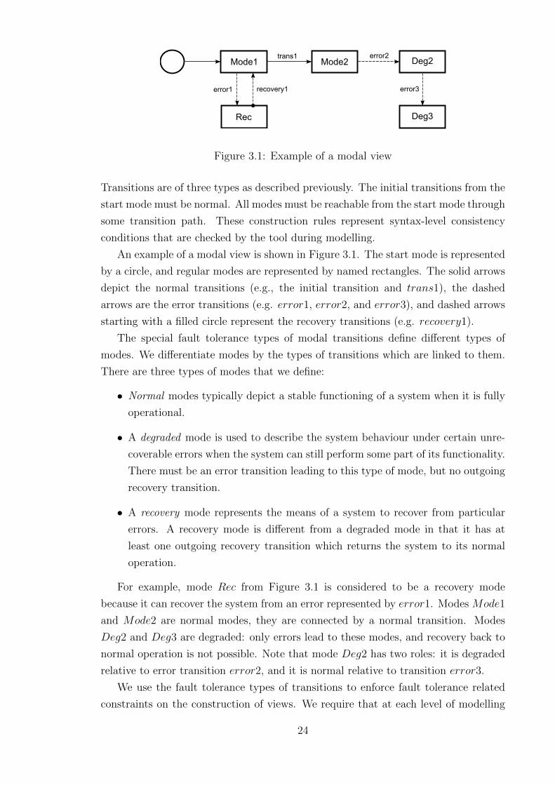
Mode1

error1

Rec

Mode2 Deg2

recovery1

trans1 error2

Deg3

error3

Figure 3.1: Example of a modal view

Transitions are of three types as described previously. The initial transitions from the

start mode must be normal. All modes must be reachable from the start mode through

some transition path. These construction rules represent syntax-level consistency

conditions that are checked by the tool during modelling.

An example of a modal view is shown in Figure 3.1. The start mode is represented

by a circle, and regular modes are represented by named rectangles. The solid arrows

depict the normal transitions (e.g., the initial transition and trans1), the dashed

arrows are the error transitions (e.g. error1, error2, and error3), and dashed arrows

starting with a filled circle represent the recovery transitions (e.g. recovery1).

The special fault tolerance types of modal transitions define different types of

modes. We differentiate modes by the types of transitions which are linked to them.

There are three types of modes that we define:

• Normal modes typically depict a stable functioning of a system when it is fully

operational.

• A degraded mode is used to describe the system behaviour under certain unre-

coverable errors when the system can still perform some part of its functionality.

There must be an error transition leading to this type of mode, but no outgoing

recovery transition.

• A recovery mode represents the means of a system to recover from particular

errors. A recovery mode is different from a degraded mode in that it has at

least one outgoing recovery transition which returns the system to its normal

operation.

For example, mode Rec from Figure 3.1 is considered to be a recovery mode

because it can recover the system from an error represented by error1. Modes Mode1

and Mode2 are normal modes, they are connected by a normal transition. Modes

Deg2 and Deg3 are degraded: only errors lead to these modes, and recovery back to

normal operation is not possible. Note that mode Deg2 has two roles: it is degraded

relative to error transition error2, and it is normal relative to transition error3.

We use the fault tolerance types of transitions to enforce fault tolerance related

constraints on the construction of views. We require that at each level of modelling

24

there must be no cycles made of error transitions. More specifically, for each mode,

if there is an error leading to some other mode and there exists a path back to the

initial mode, then that path must contain a recovery transition. Thus, one should be

able to differentiate normal from abnormal modes relative to a specific mode. E.g.,

a hypothetical transition error4 from mode Deg3 to mode Mode2 would make the

view in Figure 3.1 invalid as there would be a cycle fully made of error transitions

(error2-error3-error4). That would mean that the system could switch between the

three modes upon detection of certain errors indefinitely. Such a behaviour could not

be given a comprehensible meaning.

Besides the structural rules given in this section, there are also formal consistency

conditions described in Section 3.4.

3.3 Views Refinement

Once a modal view is in place for a particular Event-B model, it can be further re-

fined to represent changes made in successive Event-B refinement. The modal views

development process is a tree of documents much like Event-B development. There

should be no confusion between two types of refinement: a mode can only refine

another mode, and an Event-B model can only refine another Event-B model. The

view refinement process forms a tree of modal views associated with a tree of Event-B

machines (Figure 3.2).

Mi

Mi+1

Viewi

Viewi+1

Event-B refinement Modal/FT Views refinement

proof obligations

Figure 3.2: Modal views development chain

A view can refine at most one abstract view, and can be associated with at most

one model. However, the same Event-B model can be linked with any number of views,

and will have proof obligations generated for each of the linked views. Therefore,

there can be more than one view trees attached to the main Event-B development. A

25

modal view could also be abstract enough to represent a number of different systems.

The models of the systems would then be associated with equivalent views. On

the other hand, it is not mandatory to create a view for each model: a view is a

modal representation of the system, and mode refinement can be skipped for those

models that do not refine the system modal behaviour. We informally describe the

view refinement process in the next two subsections devoted to mode refinement and

transition refinement correspondingly.

3.3.1 Mode refinement rules

Each concrete mode must refine an abstract mode from an abstract view. Each

abstract mode must be refined by at least one concrete mode; it can be a one-to-

one mapping, however, the concrete mode must be expressed using the refined model

variables (see Section 3.4).

Figure 3.3 shows an example of a refinement step performed over the modal view

shown in Figure 3.1. For simplicity, only two modes Mode1 and Deg2 are refined.

Abstract mode Mode1 (shown in a dashed rectangle) is refined into three sub-modes

connected by normal transitions. Abstract degraded mode Deg2 is refined into two

sub-modes.

error1

Rec

Mode2 Deg2_1

recovery1

trans1 error2_1

Deg3

error3

Mode1_1 Mode1_2

Mode1_3

Mode1Deg2

Deg2_2error2_2

Figure 3.3: Example of a modal view refinement

Whenever an abstract mode is refined into two or more concrete modes, each of

the concrete modes depicts a more detailed and typically more deterministic part of

functionality. This is ensured by the formal conditions of refinement described in

Section 3.4.

3.3.2 Transition refinement rules

Each new transition has to refine either an abstract transition or an internal behaviour

of an abstract mode. In the first case, a transition has to connect two concrete

modes which refine two different abstract modes. The transition has to have the same

26

direction as the abstract transition. In this case, a concrete transition directly refines

an abstract transition. In Figure 3.3, error transitions error2 1 and error2 2 directly

refine abstract transition error2: they connect the concrete versions of abstract modes

Mode2 and Deg2 and maintain the direction of transition. Another example is error3

which essentially depicts two transitions from Deg2 1 and Deg2 2, and is shown to

originate from the group of the two concrete modes.

In the second refinement case, a transition can connect two concrete modes which

refine the same abstract mode. Such a transition did not exist on the abstract level

and is a refinement of the internal behaviour of an abstract mode. As an example,

abstract mode Mode1 is refined into three sub-modes. There are three (unnamed)

transitions which refine the internal behaviour of the abstract mode and become the

three explicit transitions between the concrete modes.

It is a requirement that the concrete transitions belong to either one of the two

types. We express such a requirement by the following rule: when concrete modes

are projected onto their abstract counterparts, every transition must either project

onto the internal behaviour of a mode or onto an explicitly defined transition with

the same direction.

A fault tolerance transition can be only refined by a fault tolerance transition

of the same type. This is demonstrated in the example by transitions error2 1 and

error2 2. A regular mode transition can be refined by a more specific fault tolerance

transition, but the opposite (generalisation) is not allowed.

3.4 Formalisation

The intention for the modal viewpoint is to offer a modelling assistant environment

to Event-B developers. For the approach to be useful, there needs to be a formal

relationship between a view and an Event-B model establishing that a model agrees

with a view. Thus, a modal view alone would be enough to grasp the design of modal

and fault tolerant behaviour in a model.

The formalisation approach is based on a more general notion of formal modal

systems [IRD09]. There is a study on linking modal views and Event-B [Dot+09]. The

consistency conditions discussed in this section maintain the original modal semantics

and provide developers with a practical set of proof obligations.

3.4.1 Well-definedness conditions

Mode is a general characterisation of a system behaviour. To match this notion in

terms of Event-B models, all modes and transitions are mapped into event groups.

For a stronger notion of a view - model relationship, we consider an FT view as a

set of modes providing different functionality under differing operating conditions. We

27

use the terms assumption to denote the different operating conditions and guarantee to

denote the functionality ensured by the system under the corresponding assumption.

With assumption and guarantee of a mode being predicates expressed on the same

variables as an Event-B machine, we are able to impose restrictions on the way modes

and transitions are mapped into model events and thus cross-check design decisions

in either part.

Formally, a mode is characterised by a pair A/G where:

• A(v) is an assumption - a predicate over the current system state;

• G(v, v′) is the guarantee, a relation over the current and next states of the

system; and

• vector v is the set of model variables.

It is required to show that the assumptions exhaust the invariant and thus cover

all the safe system states:

I(v)⇒ A1 ∨ A2 ∨ · · · ∨ An (COVER)

Here I(v) is a model invariant characterising valid states of v.

One other important property of a mode is that it is possible for some state

transition to take place within a mode. We do not need here to give a precise definition

of such transition because this information would be later filled in by an Event-B

machine. It is only necessary to show that there exists at least one such transition

and thus mode characterisation makes sense:

∃v, v′ · I(v) ∧ A(v)⇒ G(v, v′) (FIS)

Thus, G can never be false everywhere while, under certain circumstances, this would

be allowed for A. Note that from above it follows that a mode assumption is satisfiable:

∃v · A(v).

Each internal state transition must also preserve the machine invariant. For all

the events, such condition is satisfied by Event-B proof obligations. Being a gener-

alisation over a particular part of the machine behaviour, each mode has to preserve

the invariant as well:

I(v) ∧ A(v) ∧G(v, v′)⇒ I(v′) (INV)

In addition to modes, a view also includes transitions. Their purpose is to define

28

possible mode changes. A system switches from one mode into another through a

mode transition that non-deterministically updates the state of v in such a way that

the assumption of the source mode becomes false while the assumption of the target

mode becomes true. Let us consider two modes, i and j. A mode transition is

required to establish a new state v′ such that ¬Ai(v′) and Aj(v

′), and it is not under

the obligation to respect Gi(v, v′).

It is required that all the modes are reachable. Although we could give a formal

test for this property, there is no need in additional proof obligation - such condition

is checked by the tool at the syntax level as mentioned in Section 3.2.

3.4.2 Event-B consistency conditions

With the basic formal framework of modes in place, it is possible to define consistency

conditions for a modal view and an Event-B machine. The core principle is seeing the

view as a source of further proof obligations for a machine. We do not translate modes

into Event-B or Event-B into modes. Instead, we add additional proof obligations to

a machine that establish the consistency with a given FT view. Formally, it does

not matter where the proof obligations are added - we could prove that a machine

is consistent with a view by adding theorems to views. It is, however, more natural

to deal with additional constraints in a machine, and the intuition is that a simpler

view should lead the development of a machine. As mentioned in Section 3.3, one can

prove that the same machine is consistent with more than one view.

One can also treat the resulting Event-B model as a composition of an original

Event-B model and a view. In this respect, it is related to Event-B A, B, and in-

terface types of decomposition [Hoa+11]. With Event-B (de)composition techniques,

one horizontally splits a model into two or more models to reduce proof efforts and

improve collaborative modelling. The current approach is different from existing de-

composition techniques in that it provides orthogonal models (views) that represent

the same system-level behaviour from different “angles” as opposed to component-

wise decomposition of behaviour. Thus, a model and a view “contain” each other

through formal consistency.

The first step to formally establishing such consistency is to relate modes and

transitions to machine elements. A view is linked with an Event-B model by attribut-

ing a list of Event-B model events to each mode and each transition:

29

A1/G1 7→ E1

A2/G2 7→ E2

. . .

An/Gn 7→ En

Trans1 7→ En+1

. . .

T ransk 7→ En+k

The events which are mapped to a mode represent the internal state transitions that

may occur while the system is in that mode. Each such event must preserve the

mode guarantee and re-establish the mode assumption. The events mapped to a

transition represent different ways in which the transition may happen. Unlike modes,

the transitions are instantaneous. Thus, only one of the associated events fires while

making the transition. Therefore, every event of a transition must establish the target

mode assumption and falsify the source mode assumption as discussed earlier. Since

the same event may be associated with both a mode and more than one outgoing

transitions, the following proof obligation contains a disjunction of both conditions in

its goal:

I(v) ∧A(v) ∧H(v) ∧ S(v, v′) =⇒ [A(v′) ∧G(v, v′)] ∨ [¬A(v′) ∧ (A1(v′) ∨ . . . An(v′))]

(EVT G)

where H(v) is an event guard, S(v, v′) is an event action, A(v′)/G(v, v′) is the source

mode, A1(v′) . . . An(v′) are the target modes of a transition. The first disjunct is only

present in the obligation if the event is mapped to a mode. The second disjunct

enables one of the target modes assumptions if the event is mapped to a transition.

The ability to map an event to many modes and transitions is the difference from

the original approach to modal specifications [Dot+09]. Although this distinction

can dramatically weaken the proof obligations if overused, we allow such mapping for

practical purposes. It allows for modelling modal features of systems at abstract levels

where models typically contain non-deterministic events. Nevertheless, we assume and

suggest that system models become more deterministic during refinement, and proof

obligations generated from FT views at later refinement steps become stronger.

The next proof obligation that we describe states that the execution cannot

progress if there is no suitable enabled event for a mode or a transition. It follows that

the partitioning of the events into modes and transitions must be in agreement with

the event guards. When an event is enabled then the assumption of its mode must

hold. The same applies to a transition: the assumption of a source mode must hold

when a transition event is enabled. Since an event can be associated with multiple

30

modes and transitions, the disjunction of all the relevant assumptions must hold:

I(v) ∧H(v) =⇒ A1(v) ∨ · · · ∨ Ak(v) ∨ Atr1 ∨ · · · ∨ Atrn (EVT A)

where A1 − Ak are assumptions of the modes associated with the event, Atr1 − Atrn

are assumptions of the modes of which outgoing transitions are associated with the

event.

The requirement of execution progress also implies that at least one of the events

associated with a mode must be enabled when the system is in that mode:

I(v) ∧ A(v) =⇒ H1(v) ∨ · · · ∨Hk(v) (ENBL)

where H1(v) . . . Hk(v) are the guards of the associated events.

3.4.3 Modal views refinement conditions

Refinement rules discussed previously in Section 3.3 are complemented with additional

formal requirements. There are two proof obligations for each mode at each refinement

step. The first obligation states that the assumptions of the concrete modes must be

weaker than the abstract one:

J(v, u) ∧ A(v) =⇒ A1(u) ∧ · · · ∧ Ak(u) (REF A)

where J(v, u) is the gluing invariant containing the relation between the abstract

and concrete state variables v and u correspondingly, A(v) is the assumption of the

abstract mode, A1(u) . . . Ak(u) are the assumptions of the concrete modes.

The second obligation requires that the guarantees of the concrete modes must be

stronger than the abstract one:

J(v, u) ∧ (G1(u, u′) ∨ · · · ∨Gk(u, u′)) =⇒ G(v, v′) (REF G)

where J(v, u) is the gluing invariant, G1(u, u′) . . . Gk(u, u′) are the guarantees of the

concrete modes, G(v, v′) is the guarantee of the abstract mode.

The understanding behind the proof obligations is that during refinement we widen

the system operating conditions by weakening the assumptions, and make its be-

haviour more deterministic by strengthening the guarantees [Dot+09].

31

3.5 Conclusions and Limitations

The modal views approach is implemented as a plug-in for the industry-strength

development environment Rodin [ROD] which is based on an open extension plat-

form Eclipse [ECL]. The tool provides a view editor and seamless integration with

the Event-B development extensions such as the project explorer and the proof obli-

gation generator. The tool automatically generates verification conditions that are

necessary to ensure that a given modal view is sound and consistent with an Event-B

machine. A number of case studies have been developed using the tool to ascertain

the scalability of the method and the implementation [WIFT; LIR10]. This work

includes two industrial case studies described in the next chapters of this work.

One outcome of the experience with this environment (and the supporting tools) is

that it is generally beneficial to stratify a design into aspects, or views. This permits

a far more focused analysis and discussion of properties pertinent to a given view and

a more explicit connection to any requirements about modal and/or fault tolerance

properties.

The modal viewpoint brings benefits of explicitness and simplicity to non-formal

engineers in industry. It provides an additional type of documents which can be used

by requirements analysts and system engineers.

One of the main benefits of using the modal viewpoint is extra assurance in the

final system behaviour. The views represent an additional source of behaviour defini-

tions (along with behavioural part of the system model and safety properties) which

helps in eliminating possible mistakes and omissions. The modal views approach fol-

lows the top-down formal refinement development thus supporting the main formal

development. The views are a flexible solution for expressing orthogonal aspects of a

system which are formally consistent.

Being a positive outcome of modal views, formal consistency also requires addi-

tional proof efforts from developers. On average, the usage of modal views doubles

the number of proof obligations for those models which have one associated view. The

proportion of automatically proved obligations is approximately equal to that of the

original Event-B obligations. The complexity of those proof obligations that require

interactive proof is also similar to the original Event-B proof obligations. However,

complex views which have modes associated with large overlapping sets of events can

generate complex EVT A and ENBL proof obligations. This may be an indirect indi-

cation that the modal views are used at a very detailed level and should be simplified

(abstracted).

The possible applications of modal views are limited by their semantics. A mode

represents a possibly non-terminating behaviour, and therefore, liveness properties

cannot be expressed with a modal view. Also since a single view covers the whole sys-

32

tem behaviour, it is unreasonable to create modal views for a sequentially decomposed

system. The proposed method described in the next chapter benefits from using the

modal viewpoint for modelling reactive behaviour of systems and leaves the sequential

decomposition until later steps.

From an engineering perspective, the modal viewpoint is a flexible solution which

requires engineering decisions and experience. However, it lacks modelling guidelines

and usage patterns. The development method proposed in this thesis uses modal

views as additional restrictions to the main modelling process. We provide a number

of templates and define a development step for using the modal language.

33

Chapter 4. Development Method

In this chapter, we describe a method for top-down development of fault tolerant

systems with a focus on abstract levels of modelling. The method addresses a number

of issues of the state-of-the-art approaches that are described in Chapter 2 and is

designed to fill the existing gap in modelling and verification of abstract fault tolerant

behaviour.

The development method includes the following three constituents:

• the modelling principles stating the key points for modelling fault tolerant sys-

tems in refinement-based methods,

• the refinement strategy defining a sequence of refinement steps that need to be

performed to arrive at a meaningful model of a fault tolerant system, and

• a set of modelling patterns and modal view templates that provide a reuse mech-

anism during modelling.

The three constituents together represent modelling guidelines for building fault tol-

erant systems in refinement-based formal methods in a systematic way.

The method is designed for modelling labelled transition systems. In our method,

a system is composed of a set of states, a set of initial states, and a set of labelled

transitions between states. Each transition is a partial relation over the set of states.

The domain of a transition is defined by a domain restriction presented as a predicate.

The set of states is partitioned using variables. The method specifies particular steps

that need to be performed over the state transition system to adequately represent

the system environment and correctly model the system fault tolerant behaviour. The

guidelines proposed in this chapter can be applied during modelling in any state-based

formal method with interleaving semantics such as Action Systems [BS89], B [Abr96],

Event-B [Abr10], Z [WD96], VDM [Jon90], and TLA [Lam94].

The method consists of two parts. The first part is applicable to top-down de-

velopment of fault tolerant systems in any problem domain. It produces a reactive

system model [Ace+07] satisfying the required safety properties, and focuses on ab-

stract modelling of fault tolerant behaviour as an inherent part of system functionality.

The second part of the method is applicable to control systems. It contains guidelines

34

for modelling hardware units and implementation-level constructs such as a control

loop. This part prepares the reactive system model for implementation.

The description of the method is organised as follows. We start with stating the

basic assumptions and principles of the development method in Section 4.1. The

principles constitute a significant part of the method by underlying the key points

to be adhered during the refinement-based modelling of fault tolerant systems. In

Section 4.2 we provide a refinement strategy for modelling fault tolerant systems. We

introduce the first case study in Section 4.3 that is used throughout the chapter as a

running example to demonstrate the proposed development steps. The development

steps introduced in Section 4.2 are described in the rest of the chapter (namely, in

Sections 4.4, 4.5, 4.6, 4.7, and 4.8) and exemplified on the case study. We provide a

full list of the proposed modelling patterns and modal view templates in Section 4.9.

We finalise the chapter with conclusions in Section 4.10.

4.1 Assumptions and Principles

The development method is based on a number of assumptions and principles. We

start with an assumption that the system requirements were elicited prior to mod-

elling [HS99]. Changes to requirements during modelling can lead to (partial or com-

plete) redevelopment as it is the case with a waterfall development process [Sca02].

The main outcome of the method is a reactive model of a fault tolerant system that

satisfies the functional and fault tolerance properties stated in requirements. If the

system is a control system, then the method can be used to arrive at a detailed model

of a control system ready for implementation or code generation.

The next assumption highlights the intended outcome of the modelling process:

The ultimate purpose of modelling is to create implementable behaviour sat-

isfying the desired properties.

To satisfy the purpose, properties must be expressed in the model. These can be

safety properties expressed as invariants and proved by a theorem prover or liveness

properties to be verified by a model checker. To help developers in expressing the

desired properties, they must be easily expressible. The model should also be imple-

mentable. It should represent a behaviour that is sensible and can be implemented

and deployed in a real system. This assumption leads to a number of modelling

principles that are described in the following subsections.

35

4.1.1 Multi-view development

One of the key features of the proposed method is the usage of an additional view-

point [FKG90] that contributes to the correctness criterion for the models. The

additional viewpoint fits into state-based semantics of the target formal methods, ref-

erences the model elements, and generates a number of extra proof obligations. The

proof obligations represent an additional behaviour coverage that adds rigour to the

development process. We treat the views as collections of diagrammatically repre-

sented properties that otherwise could be difficult to express in the model, or can be

missed.

We use the the Modal / Fault Tolerance Views approach for expressing modal and

fault tolerant behaviour in separate views (see Chapter 3). A usage of the orthogonal

modal viewpoint provides three major benefits:

• The activity of system design in terms of modes, errors, and recovery transitions

gives additional understanding of the system and its modal and fault tolerant

behaviour.

• In requirements engineering, additional viewpoint represents a means for tracing

certain kinds of requirements, such as descriptions of system degradation, error

conditions, and system-level error handlers, into the formal development process.

• For engineers who are not involved in formal modelling, the diagrammatic part

of views is easier to understand than a formal model.

4.1.2 Co-refinement and restricted modelling

Refinement is a formal technique for adding details into a system model and arriving

at a model sufficiently detailed for further development steps such as implementation

or code generation. Application of formal methods, and in particular refinement, is

an engineering task. Refinement does not prescribe the exact way to model a system.

The same system can be modelled in various ways due to expressiveness of formal

notations. The criterion for a model’s usefulness is whether the model contains the

intended behaviour which satisfies the desired properties. Consider Figure 4.1. The

system behaviour must always ensure that the desired properties hold. In this regard,

properties represent the safe states of a system, but there can be more than one

behaviour satisfying the same properties.That is, the currently defined behaviour may

deviate from the intended one. By restricting the modeller’s choices, the proposed

method helps the modeller to focus on the desired behaviour and properties of the

model.

With the development process based on refinement, one starts from an abstract

model of a system that is typically non-deterministic. By making a number of steps,

36

Behaviour

Intended behaviour

Properties

Figure 4.1: Properties and behaviour

a deterministic implementable model is produced. One unveils system details through

state refinement and removes non-determinism by restricting the behaviour. Remov-

ing non-determinism is analogous to cutting off the traces of behaviour that are not

desired or irrelevant to the properties under investigation. The proposed method uses

a concept of additional views on the system model as a means to introduce restric-

tions into the modelling process. The additional restrictions remove the behaviour

that is not specified on the views thus forcing developers to make models sufficiently

deterministic.

In the method, models and views are refined in parallel and when necessary. Re-

finement of views ensures that the modal behaviour of the system becomes more

deterministic. By putting additional restrictions on the model, view refinement also

ensures that the model becomes more deterministic and still complies with the modal

and fault tolerant behaviour described in the views.

4.1.3 Behaviour restriction

In the development method proposed in this study, we see the system model as a

transition system that is “composed” of two parts: an unconstrained behaviour and a

set of functional and fault tolerance constraints. An unconstrained behaviour contains

all system states and all transitions; it is merely a declaration of the system structure

using variables. A model without constraints has a non-deterministic behaviour as it

can go from any state to any other state. Although theoretically valid, such a model

rarely has a practical application. In order for system to “behave”, i.e. realise certain

properties, we introduce constraints that define valid sets of states and transitions.

37

The constraints define the part of a transition system that is safe and sensible in the

problem domain.

We consider a transition system development as a sequence of two kinds of steps:

state refinement and behaviour restriction. A state refinement functionally redefines

a state (or a set of states) by its more detailed version that typically contains more

states. A state refinement can also add new states thus expanding the state space.

It is a top-down process of adding details to the system structure by declaring new

variables and relating them to the previously defined variables. The second type of

step, behaviour restriction, introduces new constraints and rejects previously accept-

able states and transitions. By reducing the number of transitions originating at the

same states we reduce the system non-determinism.

For example, in Event-B, state refinement is conventionally called “data refine-

ment” [Abr10] and is conducted during a vertical refinement step. Behaviour re-

striction does not have a conventional name in Event-B and is regarded as a part of

functional refinement. Here, we stress the importance of separating the two aspects of

refinement for better understanding of system behaviour and dependencies between

system components.

The method advocates modelling the abstract functionality together with fault tol-

erance in its unrestricted form first. Such a form contains elements of behaviour that

cover all possible system state changes without constraints. Additional constraints

are introduced during behaviour restriction steps to satisfy requirements. Fault tol-

erance requirements represent the constraints over the system behaviour similarly to

the functional requirements.

4.1.4 System environment

This principle is induced by our choice to use state-based formalisms for modelling

high-level system logic. The semantics that we choose for our method is interleaving

with atomic actions. It can differ from the language that is conventionally used

for expressing the system environment. For example, a physical environment of a

system would typically be of a continuous-time nature that might involve stochastic

processes. We state that an environment has to be properly abstracted in order to

create a correct model of a system:

The system environment must be adequately represented in the system model.

To represent the environment, one has to adequately model a state-based abstrac-

tion of the environment and define assumptions about the environment. The adequacy

of the model is always relative to the assumptions that we state and the purpose of

38

modelling, that is the properties that we intend to demonstrate in our model. De-

velopers may also need to refine the abstraction when using refinement-based formal

methods. Starting from the top level of development, the model inevitably contains

a certain form of abstract system environment. During refinement, both the system

and the relevant part of environment have to be specified in details.

This leads to a requirement for the developer: he/she must understand the nature

of the variables in the model, and their future implementation in the real system.

The variables may represent the logical state of the system under control, the user,

another technical system, or the system physical environment.

4.1.5 Implementable causality

In our method, we assume that a system observes some part of its environment and re-

acts to its changes. By reaction we mean any state change in the system: this includes

changes in its internal behaviour and external actions towards the environment.

All state transitions that occur during system execution need to satisfy the causal-

ity rule:

A cause should not be dependent on a reaction.

Typically, one needs to define a context of a system by explicitly separating the

system from its environment. The assumptions about the environment can be defined

explicitly as properties or implicitly using the language semantics. The causality rule

warns about a possible “trap” of modelling an environment that “waits” for system

execution without explicitly stating that as an assumption. It is acceptable when an

environment consists of another technical system that is designed to wait for the target

system. However, in many cases the system reaction must follow the environmental

cause, but not the opposite.

For example, let us define a property specifying a simple relationship between a

cause, and a reaction of a system:

cause variable = CAUSE ⇒ reaction variable = REACTION (4.1)

We assume that the cause is a part of the environment that we cannot control. To

maintain this property, both variables cause variable and reaction variable need to

be changed at the same time. We focus on modelling the system behaviour, and,

thus, our abstract representation of the environment (such as reading a sensor) con-

tains non-deterministic updates of variables. If a transition changes cause variable

non-deterministically and does not update reaction variable, it cannot be shown to

re-establish the property due to weak hypotheses. To overcome this, the domain

39

of the transition may be restricted to certain values of reaction variable. Such a

constraint would mean that in order to change variable cause variable, that repre-

sents an external phenomenon, the environment would have to wait until variable

reaction variable, that represents the system state, has a certain value. This breaks

the causality principle.

Exemplified in Event-B, this principle means that the Event-B events representing

environment must not refer to system variables in their guards. If they do, the

justification for such a design has to be given explicitly as an assumption about the

environment. Otherwise, environment events may represent false assumptions about

the real world and become unimplementable. As a result, the modelling and proving

effort becomes a mere mathematical exercise without real application.

A possible solution to this problem may include modelling the relevant part of

the environment [HJJ03; HH11] and expressing environment phenomena as a part of

system properties. However, our method focuses on modelling the system behaviour,

and only stresses the necessity to use the implementable causality principle in regard

to system environment.

4.1.6 Reactive systems and property coverage

Invariants at the current abstraction level can only cover state relationships

within a single atomic change.

By an atomic change, we understand a transition that changes all (or a part of) the

variables referenced in the property in such a way that preserves the property.

Let us consider the property defined in 4.1. If the system reaction consists of a

sequence of steps, the original property cannot be proved as it does not hold until all

steps are executed. Every step has to be covered by a finer-grained invariant; this

means that the relationship between the cause and the final system state cannot be

expressed as a single safety property at this particular level of abstraction in case of

a sequential behaviour.

Note that the atomicity refinement can still be applied, and the system-level safety

properties can be preserved during further refinement steps. However, the formal

connection between the steps of a sequence cannot be captured in safety properties

defined at the current level. Some formalisms provide means for expression of live-

ness properties as transition convergence (for example, Event-B variants). However,

this approach does not allow developers to explicitly define complex properties, and,

in practice, is mostly used for demonstration of system-level termination. To allow

developers express the necessary safety properties, we advocate the usage of abstrac-

40

tions and reactive style of modelling at higher levels and postponing the sequential

decomposition until lower levels:

For high-level modelling, it is desirable to have as few blocks of atomicity as

possible, one being an ideal case.

By reactive models we mean such definitions of behaviour that allow developers

to express high-level properties in a form cause⇒ reaction. The method proposed in

this work facilitates development of reactive models. The step for modelling a classical

control cycle of a control system is done at later stage when the reactive functionality

of the system is modelled.

4.1.7 Error modelling

Faults and the resulting errors are inevitable phenomena of the final systems [LA90].

They need to be modelled appropriately so that the system behaviour stays deter-

ministic in hazardous situations.

The proposed method focuses on modelling and refinement of abnormal system

behaviour and its environmental causes. Abnormal situations impact the system

behaviour in the same way as functional parameters do. However, such situations are

usually associated with hazardous states and severe consequences.

The method adopts error modelling from the early stages of development, and

facilitates tracing errors into requirements. Abstract errors are refined into more

specific ones; this refinement corresponds and is formally related to the appropriate

refinement of functional behaviour. For each functional level where a fault-tolerant

behaviour exists, there must be an appropriate abstraction of errors.

Errors must be abstractly modelled from the early modelling steps where func-

tionality depends on the environmental conditions.

The error modelling principle is closely related to fault injection techniques [Avr+96].

Fault injection approaches provide means for including faults to an existing model as

external entities and for checking that the system behaviour remains satisfactory. In

the proposed method, all faults originate in the system environment, and a system ob-

serves manifestations of faults through error detection. Thus, error modelling activity

is a kind of fault injection, and compliance to the error modelling principle guarantees

the formal correctness of the system behaviour in presence of injected faults.

41

4.1.8 Refinement planning

The result of a refinement-based modelling is a chain, sometimes a tree, of models.

Each level of the chain has to be in the refinement relation with the previous one. The

modeller arrives at the resulting model by exploring a tree of possible models. As each

step is associated with a proof effort, the cost of redevelopment of the abstract levels is

generally higher than that of the lower ones. To reduce the cost of redevelopment, one

needs to plan ahead by considering options for modelling certain phenomena [GIL12].

As this method focuses on fault tolerance modelling, we provide a number of modelling

practices and patterns, and formulate some modelling principles that need to be

understood when planning the refinement chain.

The system components represent various parts of the system and form a tool for

hierarchical abstraction. For example, a car engine is a component of a car and also

is a system itself with subcomponents such as valves and various sensors. During the

specification construction, components need to be defined in a top-down manner. This

is because subsystems are designed to provide certain functions to support the main

functionality of the system. For example, the process of creating a car specification

does not start with specifying the sensors’ sensitivity. The necessary and sufficient

level of sensor sensitivity is unknown until the desired properties of the engine are

defined. On the other hand, the developers need to know possible low-level solutions

in order to make decisions about high-level architecture. Such two-directional de-

pendency between levels of abstraction is an essential property in many engineering

fields including modelling. This includes refinement-based top-down formal modelling

where one needs to know possible and acceptable solutions of low-level modelling in

order to construct an abstract model.

Starting from the very abstract, models should represent system components at

appropriate abstraction levels. At the first level, the system is a single component as

a whole. The next level should introduce components that represent a decomposition

of the system, and so on. Such components as sensors, actuators, and communication

channels should be introduced at lower levels and linked formally with the abstract

components and overall system behaviour.

The same principle applies to error modelling and fault tolerance. As the desired

high-level properties of critical systems may include fault tolerance, low-level errors

need to be abstracted and included in high-level components’ behaviour. This leads

to the necessity of a pre-modelling hazard and failure analysis, an environment analy-

sis, and a possibly informal description of a system architecture. Only based on such

analysis, one is able to construct failure and error abstractions, and make high-level

decisions about the system behaviour that includes fault tolerance. Levels of abstrac-

tion at which fault tolerance is modelled need to correspond to those for functionality

as both types of behaviour are expressed in terms of the same components.

42

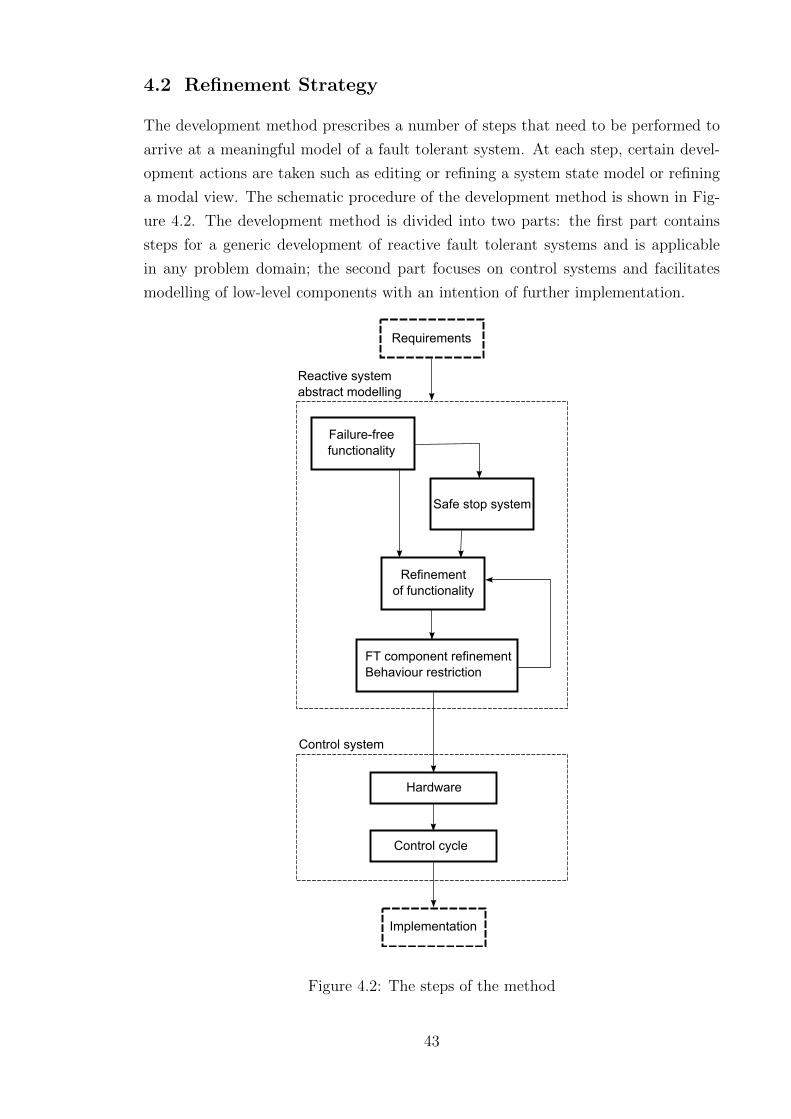
4.2 Refinement Strategy

The development method prescribes a number of steps that need to be performed to

arrive at a meaningful model of a fault tolerant system. At each step, certain devel-

opment actions are taken such as editing or refining a system state model or refining

a modal view. The schematic procedure of the development method is shown in Fig-

ure 4.2. The development method is divided into two parts: the first part contains

steps for a generic development of reactive fault tolerant systems and is applicable

in any problem domain; the second part focuses on control systems and facilitates

modelling of low-level components with an intention of further implementation.

Failure-freefunctionality

Safe stop system

Refinementof functionality

FT component refinementBehaviour restriction

Hardware

Control cycle

Reactive systemabstract modelling

Control system

Requirements

Implementation

Figure 4.2: The steps of the method

43

Abstract modelling of a reactive fault tolerant system starts with defining a failure-

free functionality of the system. By failure-free functionality we mean the abstract

behaviour only restricted by functional requirements. The abstract behaviour is then

refined and strengthened to satisfy fault tolerance requirements. At the first abstract

level where fault tolerance requirements impact the system model, a designer has to

choose an abstract fault tolerance class of the system. We define two such classes by

answering the question whether the system can mask all component errors. If the

system can eventually stop due to unrecoverable errors, then the safe stop step is

applied as a starting point for further refinement of fault tolerant behaviour.

The system functional behaviour is refined until it reaches a level of component

granularity used in fault tolerance requirements. We assume that fault tolerance

requirements enumerate component errors and describe error recovery procedures.

At this level, the system becomes aware of possible component errors and contains

appropriate reactions. The system stopped state is then refined by a combination of

component errors. At subsequent steps, component error states are further refined by

its sub-component errors etc. Thus, system functionality and component error states

stay at the same level of abstraction at all refinement steps. The functional and error

states related to a single component together comprise a fault tolerant component

in this work. Once the error states are defined for all components at the current

refinement step, the system behaviour must be restricted to contain the appropriate

reactions, i.e. fault tolerance. The modelled error states restrict the possible state

transitions of the system; this is done at the fault tolerance behaviour restriction step.

The process of alternating the two steps, functional refinement and refinement of fault

tolerance with subsequent restriction, continues until all the required properties of the

reactive system behaviour are expressed and verified.

The second part of the method refines the reactive model into a model of a control

system. The two steps performed are inclusion of low-level hardware units (sensors

and actuators) and realisation of a control cycle.

We describe each of the refinement steps in the rest of the chapter as follows.

The steps for functional development are project-specific and are left to modellers.

The discussion of the abstract fault tolerance classes of systems including the safe

stop modelling is contained in Section 4.4. The step of fault tolerance component

refinement and behaviour restriction takes the central place in the method and is split

into Section 4.5 and Section 4.6 accordingly. The refinement of system components

with sensors and actuators is described in Section 4.7. The step of implementing the

control loop of a control system is given in Section 4.8.

44

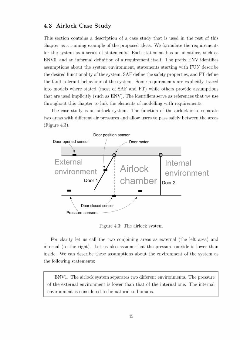
4.3 Airlock Case Study

This section contains a description of a case study that is used in the rest of this

chapter as a running example of the proposed ideas. We formulate the requirements

for the system as a series of statements. Each statement has an identifier, such as

ENV0, and an informal definition of a requirement itself. The prefix ENV identifies

assumptions about the system environment, statements starting with FUN describe

the desired functionality of the system, SAF define the safety properties, and FT define

the fault tolerant behaviour of the system. Some requirements are explicitly traced

into models where stated (most of SAF and FT) while others provide assumptions

that are used implicitly (such as ENV). The identifiers serve as references that we use

throughout this chapter to link the elements of modelling with requirements.

The case study is an airlock system. The function of the airlock is to separate

two areas with different air pressures and allow users to pass safely between the areas

(Figure 4.3).

Externalenvironment Airlock

chamber

Internalenvironment

Door 1 Door 2

Door motor

Pressure sensors

Door closed sensor

Door opened sensor

Door position sensor

Figure 4.3: The airlock system

For clarity let us call the two conjoining areas as external (the left area) and

internal (to the right). Let us also assume that the pressure outside is lower than

inside. We can describe these assumptions about the environment of the system as

the following statements:

ENV1. The airlock system separates two different environments. The pressure

of the external environment is lower than that of the internal one. The internal

environment is considered to be natural to humans.

45

ENV2. In order to maintain different pressures, the two environments must

be physically separated.

The primary function of the system can be expressed in the following form:

FUN1. When in operation, the airlock system must be able to let users pass

safely between the two environments via the airlock.

Considering ENV1-2, the system implements its function FUN1 using a number

of physical components:

ENV3. The system has two doors and a chamber. Each door when closed

separates the chamber from the appropriate environment.

ENV3 already describes a part of the solution to the problem as it defines the

components that are used to implement the desired function. Such solutions come

from domain experts and engineers. The domain knowledge should be expressed

explicitly in requirements so that they can be formalised and traced back. It is

not always practical to formally establish all properties (e.g. FUN1 is a liveness

property and can be difficult to express in proof-based methods), however, the system

architecture and abstract components such as described in ENV3 is necessary for top-

down refinement modelling. Safety requirements can be (and have to be) expressed

as invariants in the models.

Safety properties described in this section do not completely cover all safety con-

cerns that would arise for a real system. For example, a user would be required to wear

special equipment while in the chamber in order to survive the change of pressure.

We implicitly assume that this and other possible safety requirements are satisfied.

We only focus on a particular part of system properties described in this section to

limit the context of the case study.

The first safety requirement SAF1 limits the allowed range of pressure that the

system cannot exceed. Such a requirement is implied by ENV1 and ENV3:

SAF1. The pressure in the chamber must always be between the lower external

pressure and the higher internal one

Following ENV2, we can also state that it is unsafe to let a door open when the

conjoining areas have different pressures, therefore:

46

SAF2. A door can only be opened if the pressure values in the chamber and

the conjoined environment are equal

The other two safety requirements can be inferred from SAF2 and ENV1-3. Stating

them explicitly facilitates the formal modelling of ENV1 and ENV2 as well as it can

help to informally validate the requirements:

SAF3. Only one door is allowed to be opened at any moment of time

SAF4. The pressure in the chamber shall not be changed unless both doors

are closed

In order to allow a user to pass from inside through the airlock into the external

area, the system needs to perform the following steps:

1. equalise the chamber pressure to that of the internal environment,

2. open the second door to allow the user in the chamber,

3. close the second door,

4. equalize the pressure in the airlock to that of the external environment,

5. open the first door to allow the user out,

and vice versa for the opposite direction.

The components that perform these steps are described abstractly. The engineers

need to define the physical means for performing these actions such as sensors and

actuators:

ENV4. Each door is equipped with three positioning sensors and a two-way

motor. The sensors consist of two boolean sensors representing the fully closed

(SNS CLOSED) and opened (SNS OPENED) door states, and a range-value po-

sition sensor (SNS POS) that returns values in a range between the fully closed

and the fully opened states inclusively. The two-way motor (ACT MOTOR) is the

actuator that can open and close the door within its physical range of movement.

ENV5. There is a pressure sensor in each of the areas, three in total

(SNS PRESSURE OUT, SNS PRESSURE CHAMBER, SNS PRESSURE IN).

47

ENV6. The pressure in the chamber can be changed by the pump actuator

(ACT PUMP).

On top of the functional requirements to the system, we also introduce a “fragile”

environment where the physical components of the system may fail. We state this as

the following fault assumption regarding the system low-level components:

ENV7. Any of the sensors and actuators may fail to provide a correct function.

In case of critical systems, ENV7 raises another type of requirements that concerns

fault tolerance and system behaviour in a fragile environment. It is already mentioned

in FUN1 that the system performs its function “when in operation”. Under the

assumption of a fragile environment, such statement needs to be more elaborate. The

system reaction to errors has to be specified:

FT1. A system must be able to tolerate internal errors where possible and

continue its operation at an acceptable level

FT2. When errors cannot be tolerated, or it becomes dangerous to continue

operation, the system must stop in a safe state (that is already ensured by the

four safety conditions)

The system can only tolerate errors that affect redundant components. In this

case study, such redundancy is provided for the door positioning sensors:

FT3. The boolean state sensors SNS CLOSED and SNS OPENED form a

pair of devices that could be used as a hot spare for the more accurate positioning

sensor SNS POS.

When one of sensors SNS CLOSED and SNS OPENED fails, the door still re-

mains operational using the positioning sensor SNS POS, and vice versa. However,

we consider such operation dangerous in the long term, and expect the system to

gracefully degrade and finally stop for maintenance. The exact system behaviour un-

der such conditions needs to be specified, and this is an analysis task where decisions

must be made. To reason about the intended fault tolerant behaviour of the system,

we need to explicitly specify the possible hazardous situations and system reactions.

48

Such information can be obtained by applying the Failure Modes and Effects Anal-

ysis [FMTR]. In our case study, we specify the following reactions of the system to

hardware component failures:

FT4. The system should disallow opening a door if one of the corresponding

redundant sensors failed (see FT3)

FT5. The system should stop if one of the non-redundant sensors or actuators

failed

FT6. If both doors have redundant sensors failed, the system should stop as

soon as it is safe. It is considered to be safe to stop when there is no user trapped

in the chamber. If there is a user in the chamber, the system should allow opening

the internal door

In order to implement the fault-tolerant behaviour of the system, we decided to

add an additional component:

ENV8. There is a boolean-valued sensor (SNS USER) that indicates the pres-

ence of the user in the chamber

For our purpose of modelling, i.e. proof of high-level safety properties in presence

of errors, we can assume that sensor failures and appropriate system state changes

happen negligibly quick. In a method with interleaving semantics, such an assumption

allows the model to react to one error at a time. This assumption simplifies modelling

while still allows us to demonstrate the method.

It should also be noted that the method does not specify the technique of require-

ment elicitation and elaboration, it only stresses the necessity of having one. Problem

Frames [Jac01] can be one way of such reasoning about requirements.

4.4 Abstract System Fault Tolerance Classes

According to the proposed method, the first decision a developer has to make is to

choose an abstract class of a system. We define two abstract classes of systems from

the fault tolerance modelling perspective: a class of failure-free systems and a class

of safe stop systems. The differentiation between the two classes is an outcome of

a study of existing models, and is a result of a defined refinement process using the

Modal and Fault Tolerance Views’ templates (see Section 3.1 and Section 4.5.4). The

49

first class of systems is failure-free at the abstract level. It can mask all internal

errors and operates indefinitely. The second class cannot tolerate certain errors and

can eventually stop.

If the system is failure-free, its model should follow a general style for modelling

reactive systems in the target formal method. There can be a number of refinement

steps that refine abstract error-free functionality. The functionality refined at these

first steps should not involve error conditions of system components or any other en-

vironmental state that can influence the system behaviour. Typically, control systems

do not have such failure-free abstractions and their modelling should follow the safe

stop approach.

The second class of systems may stop under certain conditions that no longer

support safe system execution. The errors that can cause a system stop are called

unrecoverable and will have to be specified at later refinement steps. We do not

model the whole phenomena of the system environment and, therefore, are unable to

simulate consequences of system failures. We only focus on an implementable reaction

of a system, and consider safe stop systems. Safe stop systems can be stopped at any

moment of time to ensure safety under undesired operating conditions.

The purpose of this step is to “reserve” an abstract representation of the overall

system fault tolerant behaviour for further refinements. This step is only necessary if

the stop behaviour is refined by component failures at subsequent levels. Although safe

stop is usually the top abstraction for such systems, nothing prevents the developer

from making several steps of refinement of failure-free functionality before this step.

4.4.1 Safe stop pattern

If the safe stop abstraction is chosen for the system, the modeller has to apply the

safe stop pattern early during modelling to satisfy the error modelling principle. The

actual level for application is a designer choice. However, we suggest to introduce the

safe stop when the failure-free behaviour is specified.

Define a single variable representing the operational state of the system

(stopped). One of its values shall represent the stopped state (e.g., stopped =

TRUE). Separate the functional behaviour from the stopped state by using the

declared variable. Define a transition that switches the system to the stopped

state.

Safe stop is a special case of a more general error state variable pattern (see

Section 4.5.1). It applies to the most abstract level of fault tolerant behaviour. At

this level, we treat the whole system as a single component from the fault tolerance

perspective. The pattern assumes that the functional behaviour of the system is

50

defined on previous levels, and the system will be structurally decomposed on further

levels. The pattern explicitly separates the operational system behaviour from the

stopped state. The stop transition depicts an abstraction of unrecoverable errors.

The actual errors will be added during subsequent refinement steps.

4.4.2 Abstract modal views

Views are built in a step-wise manner, starting from the most primitive case and

introducing details along with model refinement. There are just two possible initial

views, defining the two system classes from the modelling perspective. The first class

does not have an unrecoverable error: all errors are recoverable and, at a sufficiently

abstract level, there are no errors at all. In the other case, there are errors that

cannot be masked and system necessarily transitions into a differing mode after an

error occurrence. What is considered to be an error is a design choice: the same

functionality may be implemented by either system class. Figure 4.4 illustrates the

two possible initial views.

Normal DegradedNormal

Figure 4.4: Two abstract classes of fault tolerant systems

In the first view, the most abstract system is a normal mode. Further refinements

of the view may introduce only maskable errors. In the second view, in addition to

the normal mode there is an error leading to a degraded mode. Both normal and

degraded modes may be explained in further details by introducing new maskable

errors. The error originally present in the initial view may also be explained in terms

of a number of new errors.

The abstract view of the system corresponds to the chosen fault tolerance class. As

shown in Figure 4.4, the first view represents a system with a single mode of operation.

The assumption/guarantee (A/G) pair of the mode is trivial: FALSE/TRUE. It is

valid to use such view as the first abstract depiction of the system behaviour, however,

it can be skipped in practice as it does not contribute any proofs (they are all trivially

true).

The second view is a system that can eventually stop due to unrecoverable errors.

The stop transition is an abstraction of all unrecoverable errors, and has to be refined

later. The view elements use the variables and a transition created by the safe stop

pattern. The modes shall have their A/G specified as shown in Figure 4.5.

The proposed step of modelling an abstract fault tolerance class of systems is

exemplified using our airlock example.

51

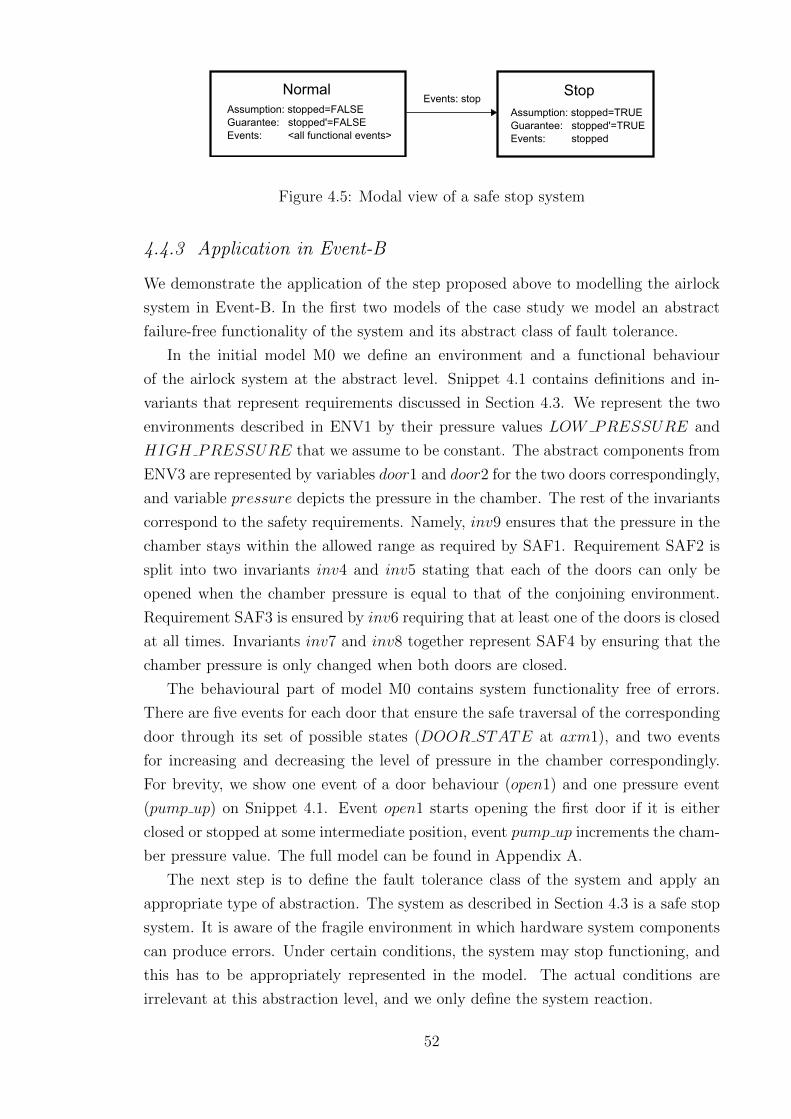
Normal StopAssumption: stopped=FALSEGuarantee: stopped'=FALSEEvents: <all functional events>

Assumption: stopped=TRUEGuarantee: stopped'=TRUEEvents: stopped

Events: stop

Figure 4.5: Modal view of a safe stop system

4.4.3 Application in Event-B

We demonstrate the application of the step proposed above to modelling the airlock

system in Event-B. In the first two models of the case study we model an abstract

failure-free functionality of the system and its abstract class of fault tolerance.

In the initial model M0 we define an environment and a functional behaviour

of the airlock system at the abstract level. Snippet 4.1 contains definitions and in-

variants that represent requirements discussed in Section 4.3. We represent the two

environments described in ENV1 by their pressure values LOW PRESSURE and

HIGH PRESSURE that we assume to be constant. The abstract components from

ENV3 are represented by variables door1 and door2 for the two doors correspondingly,

and variable pressure depicts the pressure in the chamber. The rest of the invariants

correspond to the safety requirements. Namely, inv9 ensures that the pressure in the

chamber stays within the allowed range as required by SAF1. Requirement SAF2 is

split into two invariants inv4 and inv5 stating that each of the doors can only be

opened when the chamber pressure is equal to that of the conjoining environment.

Requirement SAF3 is ensured by inv6 requiring that at least one of the doors is closed

at all times. Invariants inv7 and inv8 together represent SAF4 by ensuring that the

chamber pressure is only changed when both doors are closed.

The behavioural part of model M0 contains system functionality free of errors.

There are five events for each door that ensure the safe traversal of the corresponding

door through its set of possible states (DOOR STATE at axm1), and two events

for increasing and decreasing the level of pressure in the chamber correspondingly.

For brevity, we show one event of a door behaviour (open1) and one pressure event

(pump up) on Snippet 4.1. Event open1 starts opening the first door if it is either

closed or stopped at some intermediate position, event pump up increments the cham-

ber pressure value. The full model can be found in Appendix A.

The next step is to define the fault tolerance class of the system and apply an

appropriate type of abstraction. The system as described in Section 4.3 is a safe stop

system. It is aware of the fragile environment in which hardware system components

can produce errors. Under certain conditions, the system may stop functioning, and

this has to be appropriately represented in the model. The actual conditions are

irrelevant at this abstraction level, and we only define the system reaction.

52

axioms

axm1: partition(DOOR STATE, OPENED, CLOSED, OPENING,CLOSING, STOPPED)

axm2: LOW PRESSURE = 0

axm3: HIGH PRESSURE = 2

invariants

inv1: door1 ∈ DOOR STATE

inv2: door2 ∈ DOOR STATE

inv3: pressure ∈ Ninv4: door1 6= CLOSED⇒ pressure = LOW PRESSURE

inv5: door2 6= CLOSED⇒ pressure = HIGH PRESSURE

inv6: door1 = CLOSED ∨ door2 = CLOSED

inv7: pressure > LOW PRESSURE⇒ door1 = CLOSED

inv8: pressure < HIGH PRESSURE⇒ door2 = CLOSED

inv9: pressure ≥ LOW PRESSURE ∧ pressure ≤ HIGH PRESSURE

events

event open1 =

when

grd1: door1 = CLOSED ∨ door1 = STOPPED

grd2: pressure = LOW PRESSURE

grd3: door2 = CLOSED

then

act1: door1 := OPENING

end

event pump up =

when

grd1: door1 = CLOSED ∧ door2 = CLOSED

grd2: pressure < HIGH PRESSURE

then

act1: pressure := pressure+ 1

end

Snippet 4.1: Definitions, invariants, and behaviour of M0

53

We refine model M0 by applying the safe stop pattern. We apply the pattern

to the Event-B modelling in the following way. We define a single boolean variable

stopped ∈ BOOL. The value of the variable represents the operational availability

of the system and separates the system normal behaviour from the stopped state.

When stopped = FALSE, the system operates as defined at M0. This is ensured by

extending all functional events defined at M0 with guard stopped = FALSE. When

stopped = TRUE, the system is considered to be in the stopped state. The new

event stop puts the system in the stopped state, and represents an abstraction of

all unrecoverable errors. The new event stopped models the system behaviour in the

stopped state and has an empty action list. Because of the extended guards, the set

of functional events and event stopped do not compete and are mutually exclusive.

Thus, event stopped represents a system deadlock and guarantees that the system

will stay in the stopped state; this is sufficient for modelling the system stop [LT04b].

Snippet 4.2 shows the two new events introduced by applying the pattern and an

extension of event open1. All the 12 functional events defined at M0 are extended

similarly to open1.

invariants

inv1: stopped ∈ BOOL

events

event open1 = extends open1

when

grd stopped: stopped = FALSE

event stop =

when

grd stopped: stopped = FALSE

then

act stopped: stopped := TRUE

end

event stopped =

when

grd: stopped = TRUE

then

skip

end

Snippet 4.2: The safe stop pattern applied to model M1

Model M1 is associated with a modal view that ensures that the separation be-

tween operational and stopped modes is correct in the model. The modal view with

54

NormalStop

Assumption: stopped=FALSEGuarantee: stopped'=FALSEEvents: open1, opened1, close1, closed1, stop1, open2, opened2, close2, closed2, stop2, pump_up, pump_down

Assumption: stopped=TRUEGuarantee: stopped'=TRUEEvents: stopped

Events: stop

Figure 4.6: Modal view associated with M1

its assumption/guarantee pair and associated events is shown in Figure 4.6. It corre-

sponds to the safe stop class of fault tolerant systems.

4.5 Fault Tolerant Component Refinement

A Fault tolerant component is a structural system unit that is described by its func-

tional and error states. In this work, we assume that the fault tolerant system under

development can be represented as a layered hierarchy of fault tolerant components.

Each layer represents a level of abstraction with the system being the root of the

hierarchy. The method traverses the hierarchy starting from its root by modelling

component functional and error states at each layer. At each step, the set of compo-

nents is decomposed into its subcomponents via state refinement.

The functional refinement of components is well-known by practitioners and typi-

cally includes both data and behaviour refinements. During functional refinement, the

state representations of the higher-level components are refined by their more elabo-

rate lower-level counterparts. The behaviour of the system is refined accordingly by

specifying the allowed transitions.

In this section, we describe a refinement step for representing and refining the

component error states. The step consists in application of three modelling patterns

each described in its subsection.

4.5.1 Error state variable pattern

Each component at a current abstraction level has a functional state. For example, a

door can be opened, closed, or in an intermediate position, a boolean sensor value can

return true or false. These are the logical states of components that are necessary for

modelling the functional behaviour. To model the fault tolerant behaviour, the system

must also be aware of the availability, or error state, of its components. Examples

of such component states are “operational” and “broken”. Error states can carry

different meanings depending on the nature of the system context. In a physical

environment, error state is an abstraction over the physical state. E.g., a sensor can

be stuck, broken, or low on power supply. Such an abstraction can be derived from

the hardware specifications and/or results of reliability analysis. When the system

55

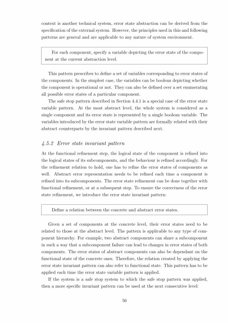
context is another technical system, error state abstraction can be derived from the

specification of the external system. However, the principles used in this and following

patterns are general and are applicable to any nature of system environment.

For each component, specify a variable depicting the error state of the compo-

nent at the current abstraction level.

This pattern prescribes to define a set of variables corresponding to error states of

the components. In the simplest case, the variables can be boolean depicting whether

the component is operational or not. They can also be defined over a set enumerating

all possible error states of a particular component.

The safe stop pattern described in Section 4.4.1 is a special case of the error state

variable pattern. At the most abstract level, the whole system is considered as a

single component and its error state is represented by a single boolean variable. The

variables introduced by the error state variable pattern are formally related with their

abstract counterparts by the invariant pattern described next.

4.5.2 Error state invariant pattern

At the functional refinement step, the logical state of the component is refined into

the logical states of its subcomponents, and the behaviour is refined accordingly. For

the refinement relation to hold, one has to refine the error states of components as

well. Abstract error representation needs to be refined each time a component is

refined into its subcomponents. The error state refinement can be done together with

functional refinement, or at a subsequent step. To ensure the correctness of the error

state refinement, we introduce the error state invariant pattern:

Define a relation between the concrete and abstract error states.

Given a set of components at the concrete level, their error states need to be

related to those at the abstract level. The pattern is applicable to any type of com-

ponent hierarchy. For example, two abstract components can share a subcomponent

in such a way that a subcomponent failure can lead to changes in error states of both

components. The error states of abstract components can also be dependant on the

functional state of the concrete ones. Therefore, the relation created by applying the

error state invariant pattern can also refer to functional state. This pattern has to be

applied each time the error state variable pattern is applied.

If the system is a safe stop system to which the safe stop pattern was applied,

then a more specific invariant pattern can be used at the next consecutive level:

56

Define a relation between the abstract stopped state and concrete component

error states. The suggested form is as follows: stopped = TRUE ⇔ Predicate.

Variable stopped is defined at the abstract level by the safe stop pattern, Predicate

is a project-specific predicate expressed in terms of the concrete component error

state variables.

The error state invariant patterns are necessary for formally establishing the rela-

tion between two subsequent layers of abstraction. Typically, refinement-based meth-

ods provide a means for expressing such a relation. In B and Event-B, this type of

relation is expressed using gluing invariants that we demonstrate later in Section 4.5.5.

4.5.3 Fault tolerant behaviour pattern

The error state variables represent the knowledge of the system about its components

conditions. At the lowest level, this knowledge comes from comparison of the current

sensor readings against the system expectations about the environment that is based

on assumptions. At all higher levels, there must be a behavioural abstraction of the

system error detection mechanisms. We represent the abstract error detection by a

number of transitions each of which corresponds to an occurrence of a certain error or

a class of errors at the current abstraction level. All errors at the current abstraction

level must be covered to satisfy the error modelling principle.

A fault tolerant system follows a detected error with an appropriate reaction. In

order to conform to the reactive systems principle, we model error detection as a

refinement of appropriate system reactions:

Every component error transition must refine the corresponding reaction tran-

sition of the system. All relevant functional states have to be covered by outgoing

error transitions.

The same error may lead to different reactions depending on the current state.

Both functional and error states are used when choosing an appropriate reaction.

Therefore, this pattern applies not only to errors but to relevant changes in the func-

tional part of the environment as well.

The fault tolerant behaviour pattern must also conform to the causality principle.

If a model has a functional state that forbids components to fail, then its behaviour

violates the causality principle. Therefore, it is mandatory to cover all possible system

conditions under which the error can be detected. In the model, this means that given

a set of errors and a set of possible system states, the resulting set of state transitions

57

will be a Cartesian product of the former two. A part of the resulting set of state tran-

sitions are modelled as error detection transitions. Those detection transitions that

lead to a system reaction specified at the abstract level should refine the appropri-

ate reaction transition. The detection transitions that represent the maskable errors

should be modelled as new transitions (they only change the state of new variables).

Some part of error state transitions can be omitted in models if there are explicitly

defined assumptions about such transitions, e.g., certain system operations can take

negligible time during which the system does not react to environmental stimuli.

After applying this pattern, the model contains all relevant detection transitions

that compete with functional transitions, both types of transitions originate at the

same states. We believe this is sufficient to adequately represent the environment in

a state machine for verifying safety properties.

4.5.4 Modal views

During the fault tolerant component refinement step, abstract components and their

errors are refined by a number of concrete subcomponents and errors. The system

behaviour is redefined in terms of subcomponent states. This allows developers to

introduce new details into the behavioural model. This is also reflected by refining

modes and splitting transitions defined on modal views.

Modes are abstractions over the overall system behaviour and not over separate

system components. Therefore, the component decomposition of the model allows a

more detailed representation of the overall system behaviour in terms of modes and

mode transitions. The refinement of modes involves both the functional and fault

tolerant system behaviour. The exact way of mode refinement is only limited by the

modal refinement conditions, and is generally project-specific.

To assist in construction of modal views, we offer two templates for modal refine-

ment. The first template is concerned with refinement of error transitions in a view.

The idea here is to replace an abstract depiction of an error with two or more concrete

errors. This process may be repeated as many times as needed and the result is a

family of errors derived from a single abstract error.

As shown in Figure 4.7, there are two versions of this template. One for the case

when an error leads to a degraded mode and another when there is also a subsequent

recovery. This distinction is due to the fact that an obligation of successful recovery

must be preserved during refinement. In the second version of the template at least

one of the recovery modes must provide a recovery transition. Thus, either one of

the recovery transitions on the second template at Figure 4.7 must remain while the

other one can be removed. For example, we can remove the recovery transition from

mode Recovery2 and still preserve the abstract recovery transition during refinement

through Recovery1.

58

Normal Degradedabstract_error

Normal

Degraded1concrete_error1

Degraded2concrete_error2

Normal Recovery

abstract_error

Normal

Recovery1concrete_error1

Recovery2concrete_error2

Figure 4.7: Error split template

In the template, error transitions are labelled with the according events that rep-

resent the transitions in the model. During refinement, the abstract error detection

event is refined by a number of lower-level component errors using the three fault tol-

erant component refinement patterns. If the definition of concrete-level errors allows

developers to refine the system modal behaviour, then the modal view can follow this

template to represent the more detailed reactions of the system to errors. As shown

on the template, the mode transitions on the two consecutive levels should contain

references to the appropriate events of the system reactions such as abstract error,

concrete error1 and concrete error2.

Mode A Mode B

Mode A

Mode B2

Mode B1

Figure 4.8: Behavioural split template

The second template is a behavioural template, it splits a system mode into a chain

of two (or possibly more) consecutive modes. This template can be used to model

intermediate operations that the system needs to perform to arrive at a supposedly

stable mode. In Figure 4.8, mode B is refined into two consecutive modes B1 and B2.

The two new transitions A→ B1 and A→ B2 refine the abstract transition whereas

transition B1→ B2 is internal and typically represents a change in a functional state

of the system. There are different applications of the template possible, however we

focus on a particular application of a functional refinement. Modes A and B2 are

assumed to be important modes in which the system is supposed to stay for long

59

periods of time, mode B1 is a temporary mode in which the system stays until some

functional condition is set to arrive at B2. Note that mode A could be refined in

a similar way. This template supports evolution of a system modal state over time,

however, the modal views language does not guarantee termination of modes.

Operation Stop

Normal StopDegraded

Figure 4.9: Graceful degradation template

A particular application of the behavioural template can be used for specifying

the system graceful degradation. As shown in Figure 4.9, a system may have one-way

transitions between a set of operational modes such as Normal and Degraded. The

chain of degradation can involve several modes and more than one path. The system

eventually stops when it encounters the conditions under which its function is not

safe. The transition to Stop can happen from any of the operational modes because

the safe stop action does not depend on the system state.

4.5.5 Application in Event-B

At M0 and M1, the system functional behaviour is defined in terms of its components.

Namely, the two doors and the airlock chamber are represented by their relevant

functional state variables. However, the system error states are defined by a single

variable stopped depicting the overall system error state.

We refine M1 by applying the fault tolerant component refinement step. Firstly,

we apply the error state variable pattern and define error states of every system com-

ponent participating in fault tolerance requirements. We introduce two error state

variables corresponding to the two doors of the airlock: door1 cond and door2 cond

as shown on Snippet 4.3. The possible door error states are

BROKEN,DEGRADED,OK. The error states are abstracted from fault toler-

ance requirements FT3-FT6 given in Section 4.3.

axioms

axm1: DOOR CONDITION = BROKEN,DEGRADED,OK

invariants

inv1: door1 cond ∈ DOOR CONDITION

60

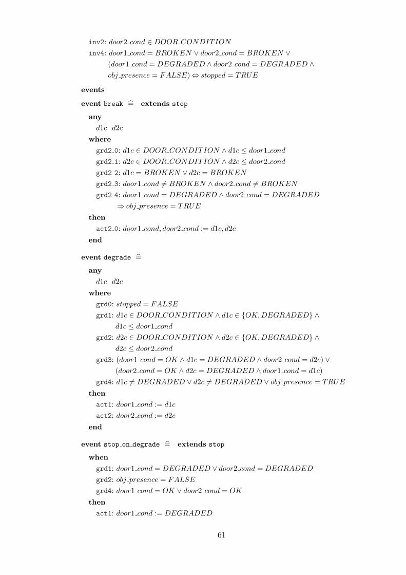
inv2: door2 cond ∈ DOOR CONDITION

inv4: door1 cond = BROKEN ∨ door2 cond = BROKEN ∨(door1 cond = DEGRADED ∧ door2 cond = DEGRADED ∧obj presence = FALSE)⇔ stopped = TRUE

events

event break = extends stop

any

d1c d2c

where

grd2 0: d1c ∈ DOOR CONDITION ∧ d1c ≤ door1 cond

grd2 1: d2c ∈ DOOR CONDITION ∧ d2c ≤ door2 cond

grd2 2: d1c = BROKEN ∨ d2c = BROKEN

grd2 3: door1 cond 6= BROKEN ∧ door2 cond 6= BROKEN

grd2 4: door1 cond = DEGRADED ∧ door2 cond = DEGRADED

⇒ obj presence = TRUE

then

act2 0: door1 cond, door2 cond := d1c, d2c

end

event degrade =

any

d1c d2c

where

grd0: stopped = FALSE

grd1: d1c ∈ DOOR CONDITION ∧ d1c ∈ OK,DEGRADED ∧d1c ≤ door1 cond

grd2: d2c ∈ DOOR CONDITION ∧ d2c ∈ OK,DEGRADED ∧d2c ≤ door2 cond

grd3: (door1 cond = OK ∧ d1c = DEGRADED ∧ door2 cond = d2c) ∨(door2 cond = OK ∧ d2c = DEGRADED ∧ door1 cond = d1c)

grd4: d1c 6= DEGRADED ∨ d2c 6= DEGRADED ∨ obj presence = TRUE

then

act1: door1 cond := d1c

act2: door2 cond := d2c

end

event stop on degrade = extends stop

when

grd1: door1 cond = DEGRADED ∨ door2 cond = DEGRADED

grd2: obj presence = FALSE

grd4: door1 cond = OK ∨ door2 cond = OK

then

act1: door1 cond := DEGRADED

61

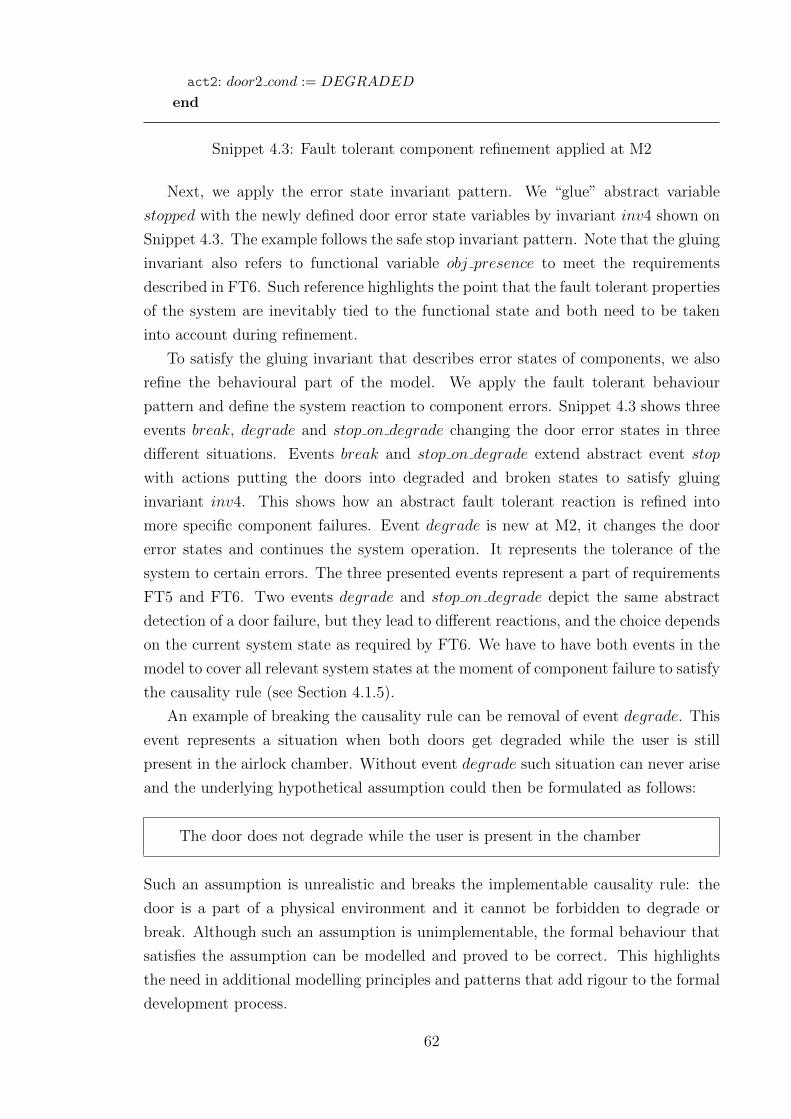
act2: door2 cond := DEGRADED

end

Snippet 4.3: Fault tolerant component refinement applied at M2

Next, we apply the error state invariant pattern. We “glue” abstract variable

stopped with the newly defined door error state variables by invariant inv4 shown on

Snippet 4.3. The example follows the safe stop invariant pattern. Note that the gluing

invariant also refers to functional variable obj presence to meet the requirements

described in FT6. Such reference highlights the point that the fault tolerant properties

of the system are inevitably tied to the functional state and both need to be taken

into account during refinement.

To satisfy the gluing invariant that describes error states of components, we also

refine the behavioural part of the model. We apply the fault tolerant behaviour

pattern and define the system reaction to component errors. Snippet 4.3 shows three

events break, degrade and stop on degrade changing the door error states in three

different situations. Events break and stop on degrade extend abstract event stop

with actions putting the doors into degraded and broken states to satisfy gluing

invariant inv4. This shows how an abstract fault tolerant reaction is refined into

more specific component failures. Event degrade is new at M2, it changes the door

error states and continues the system operation. It represents the tolerance of the

system to certain errors. The three presented events represent a part of requirements

FT5 and FT6. Two events degrade and stop on degrade depict the same abstract

detection of a door failure, but they lead to different reactions, and the choice depends

on the current system state as required by FT6. We have to have both events in the

model to cover all relevant system states at the moment of component failure to satisfy

the causality rule (see Section 4.1.5).

An example of breaking the causality rule can be removal of event degrade. This

event represents a situation when both doors get degraded while the user is still

present in the airlock chamber. Without event degrade such situation can never arise

and the underlying hypothetical assumption could then be formulated as follows:

The door does not degrade while the user is present in the chamber

Such an assumption is unrealistic and breaks the implementable causality rule: the

door is a part of a physical environment and it cannot be forbidden to degrade or

break. Although such an assumption is unimplementable, the formal behaviour that

satisfies the assumption can be modelled and proved to be correct. This highlights

the need in additional modelling principles and patterns that add rigour to the formal

development process.

62

As an example of system modal and fault tolerant behaviour refinement, we show

the modal view that is associated with M2 in Figure 4.10. It represents an application

of the graceful degradation template. The operation of the system is split into four

modes: the normal operation mode and three degraded modes. The system stays in

mode Door1 when the first door is degraded and the second door is fully operational,

and vice versa for mode Door2. When both doors are degraded and there is a user

present in the chamber, the system stays in mode Trapped until the user leaves the

chamber. The new mode Normal together with the three degraded modes formally

refine abstract mode Normal as shown by a dashed area.

The abstract system failure transition is refined by four concrete transitions de-

picting the sources of failure. Transitions Stop on degrade and User leaves initiate

at the new modes. Transition Break can initiate at any of the four modes within the

dashed area.

Normal

Door1

Door2

Trapped Stop

Break

Degrade

Degrade

Degrade

Degrade

Stop on degrade

Stop on degrade

User leaves

Figure 4.10: Modal view of airlock M2 model

The degraded modes on the view represent different sets of available components

and the associated subsets of system behaviour. The assumptions of the modes split

the possible combinations of the components error states into disjoint sets as shown

on Snippet 4.4. The mode assumptions cover all the system states as specified in the

model invariants. This is ensured by the well-definedness proof obligation COVER

(see Section 3.4).

63

assumptions

Normal: door1 cond = OK ∧ door2 cond = OK

Door1: door1 cond = DEGRADED ∧ door2 cond = OK

Door2: door1 cond = OK ∧ door2 cond = DEGRADED

Trapped: door1 cond = DEGRADED ∧ door2 cond = DEGRADED ∧obj presence = TRUE

Stop: door1 cond = BROKEN ∨ door2 cond = BROKEN ∨(door1 cond = DEGRADED ∧ door2 cond = DEGRADED ∧

obj presence = FALSE)

Snippet 4.4: M2 mode assumptions

4.6 Behaviour Restriction

The behaviour restriction step follows the fault tolerant component refinement step

described in the previous section. During this step, refined component error states

and modal views are used to restrict the functional behaviour. When applied to the

model, the step implements those fault tolerance requirements that define the changes

in system behaviour under different operating conditions. The behaviour restriction

step consists of a behaviour restriction pattern and an application of modal views.

4.6.1 Behaviour restriction pattern

The behaviour restriction pattern uses the component error states introduced by ap-

plying the error state variable pattern to restrict the functional behaviour.

Restrict the functional transitions that are not allowed with respect to the

error state variables defined earlier: use the error state variables to strengthen the

domain restriction predicates of transitions.

The error state variables represent the operational availability of components.

Under different operational conditions, system functionality may provide different

functions. For example, safety requirements might only permit a partial operation

of certain components after errors have been detected. Moreover, fault tolerance

requirements may contain specifications of different system behaviours under different

operational conditions, e.g., graceful degradation. The behaviour restriction pattern

ensures that the behavioural model satisfies such types of requirements by disallowing

functional transitions that are not valid.

The pattern should be used together with modal refinement. The modal views

provide consistency conditions that can be used to identify invalid functional tran-

sitions. Restriction predicates of relevant transitions are being strengthened using

64

this pattern to satisfy the associated modal views. In the simplest case, the con-

juncts added to domain restriction predicates of transitions take the following form:

Component condition ∈ Possible conditions, where Component condition is the er-

ror state variable for the component, and Possible conditions is a set of error states

allowing the functional transition to happen. The actual restriction predicates are

project-specific. They may involve more than one component and refer to functional

variables.

4.6.2 Modes for functionality and fault tolerance

Modal views provide a tool for specifying modal behaviour. A modal view may contain

a mixture of fault tolerant and functional behaviour as it is not always possible to

separate the two. Although a distinction between fault tolerance and functionality

can be made for a specific system, we treat the specification of modal views in a

generic way. The assumption/guarantee predicates of a mode define the nature of a

specific part of the system modal behaviour, and relationship between the system and

its environment, as well as between subsystems. Specifying assumption/guarantee

predicates is a modelling task and is specific to the system and the properties of

interest. However, we provide a general rule for specifying modes that is based on our

distinction between functional variables and error state variables.

We regard the assumption predicate as an abstraction of the system environment

that should refer to error state variables. The assumptions therefore state the com-

binations of available components that allow the system to provide its subsets of

functionality. The functionalities should refer to the logical state variables and are

contained in the guarantee predicates. Such a way of specifying the assumptions and

guarantees can be treated as a specification of the system fault tolerant behaviour.

The modal principle of providing certain functionality under the stated conditions

can be used for specifying the purely functional part of behaviour. For example, modes

can specify system operation that depends on the current logical state of one of its

components. Mode assumptions may also refer to a functional decision (represented

by a state variable) that is made by a higher-level management component. In such

cases, the views represent the functional behaviour of the system.

Although the two kinds of modal specifications can coexist in a single refinement

chain, they are usually mixed as the choice of system mode typically depends on both

component error and functional states.

4.6.3 Behaviour restriction by modal views

The modal views provide additional proof obligations. Certain model elements can

be inferred from an associated view. Such inferred elements can be offered to a user

65

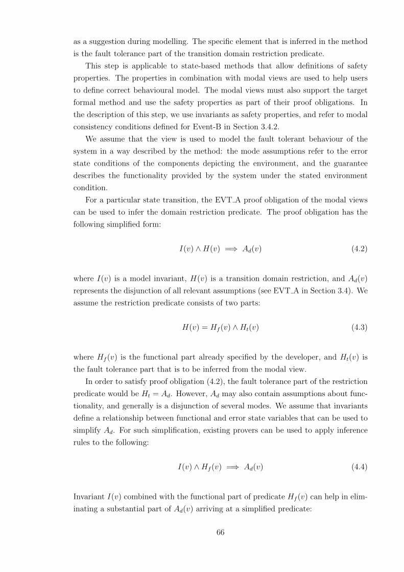
as a suggestion during modelling. The specific element that is inferred in the method

is the fault tolerance part of the transition domain restriction predicate.

This step is applicable to state-based methods that allow definitions of safety

properties. The properties in combination with modal views are used to help users

to define correct behavioural model. The modal views must also support the target

formal method and use the safety properties as part of their proof obligations. In

the description of this step, we use invariants as safety properties, and refer to modal

consistency conditions defined for Event-B in Section 3.4.2.

We assume that the view is used to model the fault tolerant behaviour of the

system in a way described by the method: the mode assumptions refer to the error

state conditions of the components depicting the environment, and the guarantee

describes the functionality provided by the system under the stated environment

condition.

For a particular state transition, the EVT A proof obligation of the modal views

can be used to infer the domain restriction predicate. The proof obligation has the

following simplified form:

I(v) ∧H(v) =⇒ Ad(v) (4.2)

where I(v) is a model invariant, H(v) is a transition domain restriction, and Ad(v)

represents the disjunction of all relevant assumptions (see EVT A in Section 3.4). We

assume the restriction predicate consists of two parts:

H(v) = Hf (v) ∧Ht(v) (4.3)

where Hf (v) is the functional part already specified by the developer, and Ht(v) is

the fault tolerance part that is to be inferred from the modal view.

In order to satisfy proof obligation (4.2), the fault tolerance part of the restriction

predicate would be Ht = Ad. However, Ad may also contain assumptions about func-

tionality, and generally is a disjunction of several modes. We assume that invariants

define a relationship between functional and error state variables that can be used to

simplify Ad. For such simplification, existing provers can be used to apply inference

rules to the following:

I(v) ∧Hf (v) =⇒ Ad(v) (4.4)

Invariant I(v) combined with the functional part of predicate Hf (v) can help in elim-

inating a substantial part of Ad(v) arriving at a simplified predicate:

66

I(v) ∧Hf (v) =⇒ A′d(v) (4.5)

The resulting predicate A′d(v) can be suggested to the user as a possible fault tolerance

part of restriction predicate Ht(v) that will satisfy EVT A.

It is possible that the suggested predicate can make the whole restriction predicate

H(v) false. Such a case signifies a contradiction between the behavioural model and

the view. Proof obligation ENBL of the modal views becomes unprovable which may

serve as an indication of the contradiction.

4.6.4 Application in Event-B

We show the behaviour restriction step applied at step M3 of the airlock case study.

The M3 modal view of the airlock describes the modal behaviour of the system under

differing error and logical conditions. The modal view is shown in Figure 4.11. We

apply the behavioural split template to modes Door1, Door2 and Trapped: we split

each of the modes into two new modes. For example, mode Door2 closing restricts

the system to only operate with the second door, and only contains events that close

or stop the door but do not open it. Upon the door closure, the system switches to

mode Door2 that guarantees that the pressure is set to low and the door is closed,

and thus only allows operating the first door.

Normal

Door1

Door2

Trapped

Door1_closing

Door2_closing

Trapped_closing_door1 Degraded

Broken

Figure 4.11: Modal view of airlock M3 model

67

Abstract mode Stop is split into two modes Broken and Degraded using the error

split template. The two modes differentiate between two different situations: the first

situation arises when the system stops upon the detection of a complete door failure,

the second situation is the safe stop due to the degraded state of both doors. The

two stop modes can also contain failure-free behaviour such as two modes of a safety

alarm although this is not modelled in the case study.

Let us focus on one of the events of the model and the modes in which it par-

ticipates. Event open1 initiates opening of the first door. It is associated with two

modes Normal and Door2. The system is in mode Normal when all components are

fully operational and, thus, the first door can be opened. The mode Door2 depicts a

situation when the second door is degraded and closed, and, thus, only the first door

can be opened. The first door cannot be opened in all other modes as it is unsafe to

do so. The A/G predicates of the two modes mentioned are shown on Snippet 4.5.

mode Normal =

Assumption: door1 cond = OK ∧ door2 cond = OK

Guarantee: TRUE

mode Door2 =

Assumption: door2 cond = DEGRADED ∧ door1 cond = OK ∧pressure = LOW PRESSURE

Guarantee: pressure′ = LOW PRESSURE ∧ door2′ = CLOSED

Snippet 4.5: The modes of M3 that can open the first door

On the previous levels, the guard of event open1 only contained functional condi-

tions of M0 and a fault tolerance condition of M1 that states that the system must be

running in order to open and close its doors. At M3, the event is restricted by error

state conditions of components derived from the modal view.

Let us apply the general form of proof obligation EV T A to event open1 (we omit

the full invariant and the guard for brevity):

I ∧H =⇒ (door1 cond = OK ∧ door2 cond = OK)∨(door2 cond = DEGRADED ∧ door1 cond = OK∧

∧pressure = LOW PRESSURE)

(4.6)

From the functional guard of the event defined at M0 we know that

pressure = LOW PRESSURE (4.7)

this simplifies the goal of (4.6):

68

I ∧H =⇒ door1 cond = OK∧(door2 cond = OK ∨ door2 cond = DEGRADED)

(4.8)

From gluing invariant inv4 at M2 we know the following:

door1 cond = BROKEN ∨ door2 cond = BROKEN∨(door1 cond = DEGRADED ∧ door2 cond = DEGRADED∧obj presence = FALSE)⇔ stopped = TRUE

(4.9)

By negating (4.9) and applying it to (4.8), we arrive at:

I ∧H =⇒ door1 cond = OK (4.10)

Thus, using the previously defined invariants and information available from the

modal view, we can suggest extending the guard of event open1 with door1 cond =

OK to satisfy the modal view. Such suggestion is inferred for every event in model

M3 given that the association between events and modes is consistent and satisfies

other proof obligations of modal views. The suggestions may contain both error state

and functional conditions. At the M3 step, we extend each of the functional events

that operate with the two doors and the chamber pump by additional guards inferred

from the associated modal view.

The current and all the previous steps facilitate the development of reactive system

behaviour that is proven to maintain the required safety properties. The following

two steps refine the abstract system model with implementation-level details. The two

steps follow the abstract reactive modelling and finalise the modelling with sequential

decomposition of the system.

4.7 Hardware

The component refinement and the behaviour restriction steps are performed in a

top-down manner until the reactive model of the system contains the required safety

properties. If the system interacts with the physical environment, then at the lowest

level the system must contain a means for such interaction. The functional and fault

tolerant behaviour obtained using the previous two steps can be further refined by

introducing hardware units such as sensors and actuators. This step is a special case

of the fault tolerant component refinement step that is applied at the lowest level of

abstraction. This step only includes the refinement of the fault tolerant part of the

system components. The functional refinement is done at the next step.

69

4.7.1 Application of fault tolerant component refinement

The components defined during the previous steps are logical and may consist of a

number of hardware units. Each of the hardware units can fail and thus the system

needs to be aware of their error states. To properly represent the hardware at the

lowest level of abstraction, we apply the error state variable pattern:

For each hardware unit (sensors, actuators, or higher level hardware compo-

nent), specify a variable depicting the error state of the unit.

The hardware error state variables have to be linked to the abstract system com-

ponents. This is done by applying the error state invariant pattern:

Define a relation between the hardware error states and abstract component

error states.

The actual gluing invariants between the error states of the abstract components

and those of the hardware units are project-specific. It is possible for the error state

of a hardware unit to contribute to a number of abstract components. The level

of abstraction used for hardware components is also project-specific. The system

behaviour can rely on complex hardware subsystems. In this case, levels of abstraction

for functionality and errors can be different.

4.7.2 Application in Event-B

At the M4 step of the airlock development, we refine one of the doors into its hard-

ware units. As required by ENV4, each door is equipped with four such units.

We model the error states of each of the sensors and the actuator by a boolean

variable as shown on Snippet 4.6. The error states of the abstract door compo-

nent need to be refined by error states of the hardware units. Gluing invariant

inv door1 sensors conditions BROKEN links the abstract BROKEN state with

appropriate combinations of the motor and the sensors. Likewise, other two states

OK and DEGRADED are refined and can be found in Appendix A. The events

that had their guards or actions referencing the door error state variables have to

be refined in terms of sensor and actuator error states. As the functional behaviour

has been restricted previously by the the behaviour restriction pattern, most of the

functional and all the detection events are refined.

The refinement of the second door component by its four hardware units is equiv-

alent to that of the first door and is omitted for brevity.

70

invariants

inv door1 pos cond: door1 pos cond ∈ BOOL

inv door1 closed cond: door1 closed cond ∈ BOOL

inv door1 opened cond: door1 opened cond ∈ BOOL

inv door1 motor cond: door1 motor cond ∈ BOOL

inv door1 sensors conditions BROKEN: door1 cond = BROKEN ⇔door1 motor cond = FALSE ∨ (door1 pos cond = FALSE ∧(door1 opened cond = FALSE ∨ door1 closed cond = FALSE))

Snippet 4.6: Error states of sensors and actuators at M4

4.8 Control Cycle

A typical control system operates in a cycle with a certain (fixed or dynamic) fre-

quency. During its operation, the control system reads the values of the sensors,

performs the control algorithm, and produces commands for the actuators in order

to control the environment. The functional state of the sensors and actuators is also

a part of the system and represents the knowledge of the system about the physical

phenomena. The actual values of the physical phenomena are unknown to the system

and can only be inferred from the sensed data.

Up to this step, the system development followed the reactive style of modelling.

As a result of applying the previous steps of the method, the system consists of

high-level functional components and their error states represented by the low-level

sensors and actuators. The functional connection between the high-level logic and low-

level values of sensors and actuators cannot be expressed using data refinement and

reactive modelling as discussed in Section 4.1.6. This step offers a modelling solution

for extending the previously developed reactive system with a sequential control cycle.

The reactive part of the system takes place during the control algorithm step of the

cycle. Sequential decomposition of the reactive model is a part of implementation -

the step does not help to specify what the system does but it specifies how the system

operates.

The control cycle step is partly derived from our previous work on incorporating

FMEA into Event-B specifications [Lop+11]. We model four phases of the cycle

and provide patterns for filling each of the phases. The major difference from our

previous work lies in the level of abstraction at which we regard it as reasonable to

apply such a sequential decomposition. In the original work, we model the control

cycle at the abstract level and leave the control logic for further refinements. Here,

we advocate a top-down approach to modelling the functionality and extend it later

with implementation-level restrictions such as a control cycle. Thus, the control cycle

extension links with the previous steps and does not clutter the reactive model of the

71

system. The patterns described in this section can also accommodate the outcomes

of the FMEA analysis, and thus the results of [Lop+11] can be reused for this work.

4.8.1 Control cycle pattern

Define a variable phase ∈ PHASE representing the current phase of the

control cycle. Define a set of four phase states that include the sensing phase, the

error detection phase, the control phase, and the prediction phase. Define four

transitions that represent the behaviour during phases correspondingly.

The control cycle pattern splits the operation of the system into four sequential steps.

During the sensing phase, the system reads the sensor values. During the second

phase, it applies the low-level error detection mechanisms. The third phase contains

the control algorithm, which is the reactive model of the system that was developed

previously. The control algorithm produces new logical components’ states and a set

of signals for the actuators. The new states and the actuator signals are used at the

final prediction phase to predict the sensor readings at the next iteration of the cycle.

The results produced by the prediction step are used by the detection mechanisms

during the next iteration.

The actual transitions for each of the phases are defined by the following four

patterns.

4.8.2 Sensing pattern

The error state variables of the system hardware units and their usage were already

defined during the previous development step (see Section 4.7). This pattern defines

the functional states of the hardware units:

Define a variable for each of the hardware units that would represent the

functional state of the unit. Non-deterministically assign a new value to the

variable during the sensing phase.

The values of the sensor variables represent the state of the sensors at the current

iteration after the sensing phase. We represent the system environment by assigning

non-deterministic values to the variables. The environment can be refined further dur-

ing later steps if necessary. We do not formally specify the environmental phenomena

such as laws of physics.

72

4.8.3 Error detection pattern

The next phase of the control cycle compares the sensor readings, which were obtained

from the sensing phase, with the allowed range of values. The detection phase returns

the detected hardware error states that are then used by the control algorithm.

The first step to implementing the detection mechanism is defining the variables

necessary for correct refinement of the abstract model:

Define a variable for each of the hardware units that would represent the error

state as detected by the error detection phase. Assign new values to the variables

based on the sensor readings introduced by the sensing pattern, last known sensor

error states, and sensor values produced by the prediction pattern during the

previous iteration.

The detected error state variables are a copy of the sensor error state variables

defined by the hardware pattern (see Section 4.7). The new error state variables are

required for the error detection phase to ensure the correct refinement of the abstract

reactive model.

The newly defined variables are assigned new values by detection transition

cycle detect. The assignments represent the detection mechanisms used by the sys-

tem. We define several types of low-level error detection mechanisms based on the

sources of information for the detection:

• the sensor reading may be compared against the statically defined acceptable

range of values;

• the system may expect a certain value from the sensor reading that is based on

the previous iteration of the cycle;

• the sensor reading may be compared to the active redundant sensors.

There may be other types of error checks depending on the system, we do not

intend to cover all possible error detection mechanisms. Error detection at this level

of abstraction is done sequentially as opposed to the abstract error detection described

in Section 4.5.3.

4.8.4 Control phase patterns

We represent the control phase by the reactive behaviour of the system that is de-

veloped using the previous method steps. The reactive model of the system contains

transitions that change the hardware error states and represent the system fault tol-

erance. The results of the detection phase of the control cycle are used here to feed

73

the obtained hardware error states to the reactive behaviour. Similarly, the sensor

readings are used by the functional part of the system to ensure that the sensor values

match the abstract logical state of the components.

The functional control phase pattern:

Restrict the functional transitions with additional domain restriction that spec-

ifies the sensor values necessary for the execution of the transition. The domain re-

striction has to be of the following form: sensor cond = TRUE⇒P (sensor value)

where sensor cond is the hardware error state variable, and P (sensor value) is a

predicate over the acceptable sensor values. The functional control phase pattern

ensures that the value of the sensor is only used when the sensor is in a working

condition hence the implication. The added restriction predicate models the relation

between the concrete-level hardware units and the abstract component states.

The fault tolerant control phase pattern ensures that the abstract error detection

is refined to use the information obtained from the detection phase:

Restrict the domain of error detection transitions to include the previously

detected hardware error states. Use the detected states as new values for abstract

error states.

At the abstract level, error detection transitions represented the environment as a

non-deterministic choice between different errors. This pattern restricts the detection

transitions by using the detected error states, thereby providing a place for imple-

menting the detection mechanisms.

During the control algorithm, the reactive behaviour of the system uses the sensor

readings and the error state variables to change its logical state and produce signals

for the actuators. The actuators are assumed to receive the signals instantly.

4.8.5 Prediction phase pattern

The last phase of the control cycle produces the expectations of the system about the

sensor states at the next iteration.

Define a prediction variable for each of the sensor values. Assign the predicted

value at the last phase of the control cycle.

Thus, the variables defined are a copy of the sensor value variables with the same

types. The prediction represents the assumptions about the environmental phenom-

ena, and the expectation of the system about the next state of its components. The

74

prediction variables are then used at the detection phase by the error detection pat-

tern.

This is the last step of the method. After this step, the system is sufficiently

detailed and can be used for implementation. The implementation can be manual

or automated for a particular family of models that incorporate the control system

patterns. The resulting formal specification can also be used for test-case generation

to ensure correctness of the final code.

4.8.6 Application in Event-B

We exemplify the five patterns described in this section in Event-B and demonstrate

their application on the airlock case study. Firstly, we instantiate the control cycle

pattern by defining the four events of a control cycle as shown on Snippet 4.7. The

events represent the four control cycle phases as described in Section 4.8.1. This is

ensured by guards grd phase and actions act phase.

axioms

axm1: partition(PHASE, ENV , DET, CONT, PRED)

invariants

inv phase: phase ∈ PHASE

inv1: door1 pos ∈ Zinv2: door1 opened ∈ BOOL

inv3: door1 closed ∈ BOOL

inv4: door1 pos predicted ∈ Zinv5: door1 opened predicted ∈ BOOL

inv6: door1 closed predicted ∈ BOOL

inv7: door1 motor ∈ −1, 0, 1inv10: door1 pos cond detected ∈ BOOL

events

event cycle sense =

when

grd phase: phase = ENV

grd stopped: stopped = FALSE

then

act phase: phase := DET

act5 1: door1 pos :∈ Zact5 2: door1 opened :∈ BOOL

act5 3: door1 closed :∈ BOOL

end

event cycle detect =

75

when

grd phase: phase = DET

grd stopped: stopped = FALSE

then

act phase: phase := CONT

act5 1: door1 pos cond detected := bool(door1 pos cond = TRUE ∧(min door ≤ door1 pos ∧ door1 pos ≤ max door) ∧(door1 opened cond = TRUE ∧ door1 opened = TRUE⇒

door1 pos = max door) ∧(door1 closed cond = TRUE ∧ door1 closed = TRUE⇒

door1 pos = min door) ∧(door1 pos = door1 pos predicted))

end

event open1 = extends open1

when

grd phase: phase = CONT

grd pos: door1 pos cond = TRUE⇒ door1 pos < max door ∧(door1 pos = min door⇒ door1 = CLOSED) ∧(door1 pos > min door⇒ door1 = STOPPED)

grd closed: door1 closed cond = TRUE⇒(door1 closed = TRUE⇒ door1 = CLOSED)

grd opened: door1 opened cond = TRUE⇒ door1 opened = FALSE

then

act phase: phase := PRED

act motor: door1 motor := 1

end

event degrade door1 = refines degrade door1

when

grd phase: phase = CONT

grd degradation: (door1 pos cond detected = FALSE ∧ door1 pos cond =

TRUE) ∨(door1 closed cond detected = FALSE ∧ door1 closed cond = TRUE) ∨(door1 opened cond detected = FALSE ∧ door1 opened cond = TRUE) ∨(door1 motor cond detected = FALSE ∧ door1 motor cond = TRUE)

grd stopped: stopped = FALSE

grd1: door1 pos cond = TRUE ∧ door1 closed cond = TRUE ∧door1 opened cond = TRUE ∧ door1 motor cond = TRUE

grd7: door2 cond = DEGRADED⇒ obj presence = TRUE

grd glue: door1 motor cond detected = TRUE ∧((door1 pos cond detected = FALSE ∧ door1 opened cond detected =

TRUE ∧door1 closed cond detected = TRUE) ∨

76

(door1 pos cond detected = TRUE ∧(door1 opened cond detected = FALSE ∨door1 closed cond detected =

FALSE)))

with

pos cond : pos cond = door1 pos cond detected

opened cond : opened cond = door1 opened cond detected

closed cond : closed cond = door1 closed cond detected

motor cond : motor cond = door1 motor cond detected

then

act phase: phase := PRED

act5 0: door1 pos cond := door1 pos cond detected

act5 1: door1 closed cond := door1 closed cond detected

act5 2: door1 opened cond := door1 opened cond detected

act5 3: door1 motor cond := door1 motor cond detected

end

event cycle predict =

when

grd phase: phase = PRED

grd stopped: stopped = FALSE

then

act phase: phase := ENV

act5 1: door1 pos predicted := door1 pos+ door1 motor

act5 2: door1 opened predicted := bool(

(door1 motor = 1 ∧ door1 pos = max door − 1) ∨(door1 motor = 0 ∧ door1 opened = TRUE))

act5 3: door1 closed predicted := bool(

(door1 motor = −1 ∧ door1 pos = min door + 1) ∨(door1 motor = 0 ∧ door1 closed = TRUE))

end

Snippet 4.7: Modelling the control cycle at M5

We apply the sensing pattern and define four variables representing the sensed

values of the hardware units. We only model the hardware units of the first door

as required by ENV4. Sensor door1 pos returns the position of the door that is

represented as an integer value (see inv1). Sensors door1 opened and door1 closed

are boolean sensors at the two extreme positions of the door (inv2 and inv3 cor-

respondingly). The signal for actuator door1 motor represents the direction of the

door movement: −1 for closing, 1 for opening, and 0 for stable position (inv7). The

sensing phase of the control cycle is represented by event cycle sense. It assigns ar-

77

bitrary values to the sensor readings as we do not formally model the environmental

phenomena.

At the next phase, the system executes its error detection mechanisms represented

by event cycle detect. Snippet 4.7 shows an example of error detection for the posi-

tioning sensor of the first door. The error detection for the sensor includes the three

types of detection mechanisms, and ensures that once the sensor failure is detected,

the value will be kept during all subsequent iterations.

Once the hardware functional and error states are obtained, they are used dur-

ing control phase to execute the system functional and fault tolerant behaviour. For

example, we apply the functional control phase pattern and extend functional event

open1 with additional guards (grd pos, grd closed, and grd opened) stating the ex-

pected functional and error states. The event now also produces a signal to the motor

actuator by its action act motor. An example of applying the fault tolerant control

phase pattern is a refinement of detection event degrade door1 shown on Snippet 4.7.

The event now contains a number of guards that use the values obtained during the

error detection phase to refine the previously non-deterministic error detection. Event

actions directly assign the detected values to the error state variables defined during

reactive modelling. The refinement relation is formally ensured by providing new

detected values as event witnesses.

The last phase of the control cycle is the prediction phase. On Snippet 4.7, we show

the predictions of the next expected states of the three sensors in event cycle predict.

For example, sensor door1 pos is expected to change its value according to the signal

given to the motor, and return door1 pos+ door1 motor during the next iteration.

The application of the control cycle step finalises the modelling of the airlock

system, and provides placeholders in the model for further implementation.

78

4.9 Summary of Patterns

We provide a summary of modelling patterns and modal view templates that are used

by the method in Table 4.1. The patterns are described in details in corresponding

sections of this chapter as provided in the table.

Name Section Description

Safe stop pattern 4.4.1 A starting point for modelling fault tolerant behaviour.

Introduced model elements are refined at later steps

Error state vari-

able pattern

4.5.1 Defines representation of components error state

Error state invari-

ant pattern

4.5.2 Links components error state at the current level with

the abstract component

Fault tolerant be-

haviour pattern

4.5.3 Defines behaviour of the environment and ensures the

appropriate system reaction

Behaviour restric-

tion pattern

4.6.1 Restricts the functional behaviour with fault tolerance

constraints

Control cycle pat-

tern

4.8.1 Introduces a control loop by sequentially decomposing

the model

Sensing pattern 4.8.2 Defines functional states of sensors and actuators, and

the sensing phase of the control loop

Error detection

pattern

4.8.3 Defines the error detection phase of the control loop and

variables that represent the detected error states of the

components

Functional con-

trol phase pattern

4.8.4 Links the reactive functionality with the sensor values

obtained during the sensing phase

Fault tolerant

control phase

pattern

4.8.4 Refines the abstract representation of errors by values

that were obtained during the detection phase

Prediction phase

pattern

4.8.5 Defines the prediction phase of the control loop and vari-

ables that represent expectations of the system about the

future functional states of components

Error split tem-

plate

4.5.4 Splits an abstract error transition (and associated recov-

ery and degraded modes) into two or more concrete errors

Behavioural split

template

4.5.4 Refines an abstract mode by a sequence of two modes,

introduces an intermediate mode

Graceful degrada-

tion template

4.5.4 Extends a system operation mode with a sequence of de-

graded modes

Table 4.1: Summary of proposed patterns

79

4.10 Conclusions

In this chapter, we proposed a method for top-down development of fault tolerant

systems. The method focuses on a notion of fault tolerant component and provides

a modelling solution to connecting the refinement of component errors with system

functionality through behaviour restriction.

We described the modelling principles and assumptions that should be adhered

to during modelling. Based on the principles, we proposed a refinement strategy for

building reactive models of systems and further sequential decomposition leading to

implementation of control systems. We identified a number of patterns that support

the refinement strategy throughout the chapter, and provided a summary of all the

modelling patterns and modal view templates.

We demonstrated the proposed method on a medium-scale case study. The air-

lock system has been modelled using the Rodin development environment and the

associated plug-ins for Event-B model transformations and modal views modelling.

To evaluate the method and the tools, we model another case study from a different

domain that we describe in the next chapter.

80

Chapter 5. Evaluation

The aim of this chapter is to report on evaluation of the method proposed in Chap-

ter 4. The evaluation process consists in applying the proposed steps of the method

to developing an industrial case study. By developing the system, we validate the

research hypotheses which we reprise in the following statements:

• The method supports and encourages top-down specification of fault tolerant

system behaviour with the purpose of correct design of system fault tolerance

in a refinement-based formal method

• The method provides a general refinement strategy which specifies the steps

that need to be taken to arrive at a correct model of a fault tolerant system

• The refinement strategy is derived from modelling principles and is supported

by modelling patterns

• The method provides facilities for explicit modelling of fault tolerance

• The method maintains the applicability of the formal method to modelling the

system functionality, and allows for smooth integration of functionality with

fault tolerant behaviour

To support the evaluation statements, we model the Attitude and Orbit Control

System (AOCS) case study. This is a medium-scale control system which was inde-

pendently developed by several industrial companies from the aerospace domain. One

of them is Space Systems Finland (SSF) [SSF] which was one of four industrial part-

ners of the DEPLOY project. We define our simplified requirements for the system

based on project deliverable [D3.1] and associated internal requirements documents.

The chapter is organised as follows. We introduce the requirements for the AOCS

system in Section 5.1, then we provide the relevant parts of the models and describe

the steps performed during modelling in Section 5.2, and we summarise our evaluation

in Section 5.3.

81

5.1 Requirements for AOCS

In this section, we present the requirements for the AOCS system that we use during

the modelling process.

The Attitude and Orbit Control System (AOCS) [D3.1] is a generic component of

a satellite onboard software operating in the following environment:

ENV1. The environment of the AOCS consists of the physical phenomena of

Newtonian dynamics applied to the object in orbit around the Earth, and other

phenomena measured by the payload instrument.

The main function of the AOCS is defined as follows:

FUN1. The AOCS is a control system which ensures the desired attitude and

orbit of a satellite. The control is necessary for the payload instrument to fulfil

its mission.

Due to the tendency of a satellite to change its orientation because of disturbances

from the environment, the attitude needs to be continuously monitored and adjusted.

An optimal attitude is required to support the needs of payload instruments. For

example, attitude control may ensure that an optical system of the spacecraft will

continuously cover the required area on the ground. To fulfil the mission the AOCS

is controlling a number of hardware units of the satellite:

ENV2. The AOCS is equipped with three hardware units: the Earth sensor

(ES) gives the distance and the orientation relative to the Earth, the GPS sensor

provides the GPS coordinates of the satellite, and the Payload instrument (PLI)

fulfils the mission of the satellite by reading the relevant information from the

environment.

The AOCS uses the ES and GPS hardware units to keep the satellite on a desired

trajectory. The operation of the AOCS is mode-based which is described by FUN2:

FUN2. The AOCS can operate in a number of system modes. Each system

mode is associated with a set of required unit modes. The ultimate function of the

AOCS is to acquire the best possible system mode where the payload instrument

is gathering its data.

82

Off

Science

Nominal

all units: OFF

ES: ONGPS: COARSEPLI: OFF

ES: OFFGPS: FINEPLI: ON

Figure 5.1: AOCS system modes

In this case study, a satellite can be in three operational modes: Off, Nominal,

and Science. The satellite is in the Off mode from the moment separation from the

launcher is achieved. In this mode the AOCS is not operational; this mode is regarded

as a preparatory phase. From the Off mode, the AOCS progresses to modes where

more sensors are involved. The next mode to switch to is Nominal; in this mode the

ES and GPS units are switched on, and the satellite acquires and preserves a stable

attitude. The overall aim is to enter and stay in the Science mode where fine GPS

positioning is achieved and scientific instruments (PLI units) are reporting readings.

The described mode switching behaviour is a requirement that can be captured as a

diagram shown in Figure 5.1.

Similar to the airlock example, the AOCS also operates in a fragile environment:

ENV3. Any of the satellite units can fail to provide its service.

To tolerate such faults, the system hardware is provided with redundancy:

ENV4. Each unit is supported by a redundant cold spare which can be used

when the main unit fails.

The AOCS is expected to handle the control algorithm related errors (such as

attitude computation errors) and the unit errors (including all errors related to loss

of accuracy, invalid data, etc.). Such errors may happen at any moment of time

including the transition phase between modes.

FT1. Upon the detection of any unit error, the AOCS must degrade to a lower

mode in which the failed unit is not used. The failed unit must be replaced with

83

its spare. When the spare unit fails, the AOCS is no longer permitted to operate

in those modes which use the failed type of unit.

For example, if both PLI units fail, the satellite can no longer operate in the

Science mode, and is forced to stay in the Nominal mode. At the moment of failure,

the system must degrade to a lower mode which is shown by backward transitions in

Figure 5.1.

The requirements for the AOCS case study are derived from one of the DEPLOY

project deliverables in space sector [D3.1]. The deliverable and related documents

contain an industrial description of the AOCS system. The industrial requirements

are simplified for clarity of the present work. Namely, the five modes of the original

system are reduced to three in the case study due to their generic representation

in the model. Attitude errors of the original system are not present in the case

study because they are treated in our method as a type of transition errors. We

further simplify the requirements by removing the concepts of mode, unit, and FDIR

managers. We believe that the mentioned concepts represent software components,

i.e. implementation, and should not be considered by our method.

Although AOCS is a control system, we do not intend to model the actual control

algorithm. We focus on high-level logic of modal and fault tolerant behaviour of the

system for evaluation purposes. The proposed case study was chosen and is adequate

for evaluation of the method for the following reasons:

• It contains realistic requirements derived from industrial documents

• AOCS is a critical system and, therefore, needs to tolerate faults during its op-

eration. Requirements include fault tolerance in a form of graceful degradation

which cross-cuts the functionality

• As shown later, all the method steps for modelling reactive fault tolerant systems

can be exemplified during modelling AOCS

• The system is mode-based, which allows us to evaluate the applicability of

Mode/FT Views

The case study is limited to modelling a particular component of a real system

specification. There may be certain relevant behaviour of the rest of the system that

is not modelled here. For example, we focus on the abstract development of reactive

modal behaviour of the AOCS and do not model the actual control algorithm. Also,

the case study does not fully demonstrate the usefulness of event guard suggestions

described in Section 4.6.3. This is due to inherently modal nature of the case study.

84

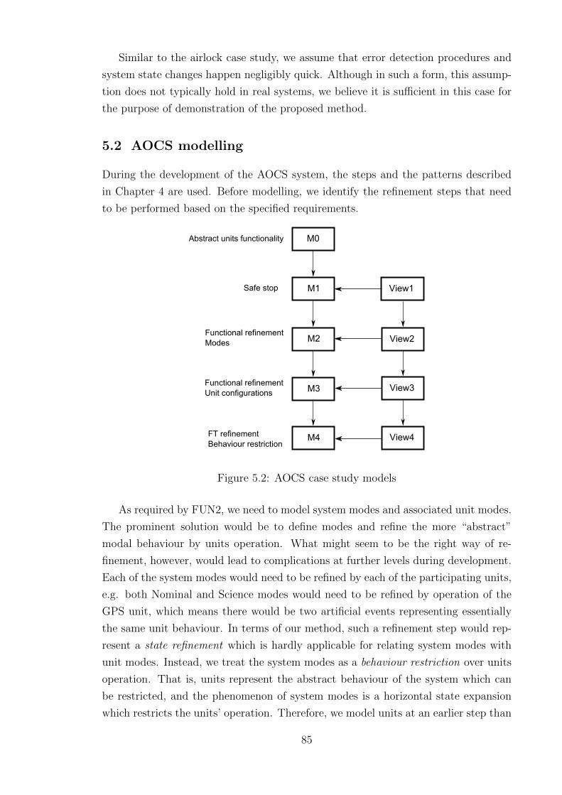
Similar to the airlock case study, we assume that error detection procedures and

system state changes happen negligibly quick. Although in such a form, this assump-

tion does not typically hold in real systems, we believe it is sufficient in this case for

the purpose of demonstration of the proposed method.

5.2 AOCS modelling

During the development of the AOCS system, the steps and the patterns described

in Chapter 4 are used. Before modelling, we identify the refinement steps that need

to be performed based on the specified requirements.

M0

M1 View1

M2

M3

M4

View2

View3

View4

Abstract units functionality

Safe stop

Functional refinementModes

Functional refinementUnit configurations

FT refinementBehaviour restriction

Figure 5.2: AOCS case study models

As required by FUN2, we need to model system modes and associated unit modes.

The prominent solution would be to define modes and refine the more “abstract”

modal behaviour by units operation. What might seem to be the right way of re-

finement, however, would lead to complications at further levels during development.

Each of the system modes would need to be refined by each of the participating units,

e.g. both Nominal and Science modes would need to be refined by operation of the

GPS unit, which means there would be two artificial events representing essentially

the same unit behaviour. In terms of our method, such a refinement step would rep-

resent a state refinement which is hardly applicable for relating system modes with

unit modes. Instead, we treat the system modes as a behaviour restriction over units

operation. That is, units represent the abstract behaviour of the system which can

be restricted, and the phenomenon of system modes is a horizontal state expansion

which restricts the units’ operation. Therefore, we model units at an earlier step than

85

we do modes. We conduct the same planning for the fault tolerant part of the system

behaviour: we further restrict the units operation by detecting and acting upon unit

errors. Following the method steps, unit errors need to refine the abstract system

failure, therefore, we need to introduce safe stop before we model unit errors. This

example shows the necessity of (informal) refinement planning.

Using our reasoning about the system components and behaviour which need to

be modelled, we define the refinement steps which are shown in Figure 5.2. The

model of the AOCS case study includes five Event-B machines and four modal views.

We start with modelling the abstract unit functionality at M0 which is described in

Section 5.2.1. Then we introduce a system safe stop at M1 which is briefly discussed

in Section 5.2.2. We conduct functional refinement at levels M2 and M3 and intro-

duce modes and unit reconfiguration which is discussed in Section 5.2.3. Model M4

refines the AOCS safe stop into unit errors, and uses them to restrict the functional

behaviour. We split the description of M4 into two sections: the fault tolerant com-

ponent refinement is discussed in Section 5.2.5 and the behaviour restriction step is

discussed in Section 5.2.6.

5.2.1 Functional model M0

The first model of the AOCS case study contains the abstract functionality of the

system. It corresponds to the failure-free step of the proposed development method.

The model defines the functional states of the three system units. The functionality

of each unit is abstractly modelled by two events: event work corresponds to the

unit operation, and event switch represents the switch of the unit between functional

states. Snippet 5.1 shows the two events for the ES unit. The units GPS and PLI are

represented similarly.

We omit modelling the actual control algorithm because such modelling should

be either postponed until later steps or modelled using continuous-time notations.

Therefore, events work for the three units contain no actions, they represent a mere

fact that the units perform something useful when in operation.

At this stage, the model only represents the ability of the units to perform their

function and switch between their modes which is required by ENV2. The model

corresponds to the failure-free functionality step of the method. The units operation

and switching between unit modes is the most abstract unrestricted functionality that

covers any possible combination of units. All further refinements introduce restrictions

in a form of disallowing certain units to operate or switch as a result of functional

and environmental causes.

86

axioms

axm1: UNIT OFF = 0

axm2: UNIT ON = 1

axm3: GPS COARSE = 1

axm4: GPS FINE = 2

invariants

inv1: unitES ∈ UNIT ON,UNIT OFFinv2: unitGPS ∈ UNIT OFF,GPS COARSE,GPS FINEinv3: unitPLI ∈ UNIT OFF,UNIT ON

events

event ES work =

when

grd1: unitES = UNIT ON

then

skip

end

event ES switch =

any

newState

where

grd1: newState ∈ UNIT ON,UNIT OFFgrd2: newState 6= unitES

then

act1: unitES := newState

end

Snippet 5.1: AOCS model M0

5.2.2 Safe stop at M1

AOCS is a safe stop system in terms of the controlled units. When a unit fails in

such a way that the system can no longer operate, it switches to the stop mode which

depicts a safe mode where none of the three units are required.

At the M1 modelling step we apply the safe stop step described in Section 4.4.

The Event-B model is extended according to the safe stop pattern, and the modal

view of the system follows the safe stop template and contains two modes: Operation

and Stop. This step is required because we plan to refine the safe stop by unit errors

at one of the next refinement levels.

87

5.2.3 Functional refinement at M2

At the next two steps M2 and M3 we restrict the unit switching events by modelling

the AOCS system modes of operation. First, we introduce the system modes and

transitions, and restrict the units operation by modal requirements. On the next level

we restrict the modes reconfiguration process by ensuring that the reconfiguration

takes place until all units switch to their appropriate modes. In terms of our method,

M2 contains a state refinement and a behaviour restriction step, and M3 contains a

behaviour restriction step towards system reconfiguration. The refinement steps M2

and M3 also demonstrate how the modal views are applied to modelling of functional

behaviour.

invariants

inv1: stable ∈ BOOL

inv2: mode ∈MODE

events

event goAdvance =

when

grd stopped: stopped = FALSE

grd1: stable = TRUE

grd2: mode < SCIENCE

then

act1: mode := mode+ 1

act2: stable := FALSE

end

event downgrade =

any

newMode

where

grd stopped: stopped = FALSE

grd par: newMode ∈MODE

grd1: mode > OFF

grd2: newMode < mode

then

act1: mode := newMode

act2: stable := FALSE

end

Snippet 5.2: Introducing AOCS system modes at M2

At M2 we introduce the system modes and the process of system reconfiguration.

88

As shown on Snippet 5.2, we define two new events goAdvance and downgrade that

represent the initiation of the reconfiguration process. State variables mode and

stable describe the current mode of operation. When stable = FALSE, variable

mode contains the target mode for the reconfiguration. When stable = TRUE, the

system invokes the units functionality as required by a particular mode. So far, the

only functional property that M2 provides is the behavioural ability to switch between

modes. However, system modes do not define any formal relationship with unit modes

- the reconfiguration process is modelled in its unrestricted form.

In order to meet the requirement FUN2, we need to associate system modes with

appropriate subsets of units. We apply the behaviour restriction step to the functional

behaviour and restrict units operation to allowed subsets of modes. For example, unit

ES is required to switch on and work in the Nominal system mode and should be

switched off in any other mode (Snippet 5.3). This is a direct application of the

behaviour restriction pattern where instead of error state variables we use a part of

the functional behaviour (system modes).

events

event ES work = extends ES work

when

grd mode: mode = NOMINAL

then

skip

end

event ES switch on = refines ES switch

when

grd stopped: stopped = FALSE

grd1: unitES = UNIT OFF

grd2: mode = NOMINAL

with

newState: newState = UNIT ON

then

act1: unitES := UNIT ON

end

Snippet 5.3: Adding functional modes at M2

The modal view of M2 reflects the introduced modes of operation as shown in

Figure 5.3. Three modes Off, Nominal and Science refine abstract mode Operation.

The assumptions of the modes are of form mode =< MODE >, where < MODE >

is substituted for specific mode constants accordingly. The modes refer to the appro-

priate unit events. For example, mode Nominal only allows operation for the ES and

89

Off

Science

Nominal Stop

Figure 5.3: Modal view of AOCS M2 model

mode Nominal =

Assumption: mode = NOMINAL ∧ stopped = FALSE

Guarantee: stopped′ = FALSE

Events: GPS switch off, PLI switch off,ES switch on,GPS switch on,

ES work,GPS work, reconf finish

Snippet 5.4: The Nominal mode of the AOCS M2

GPS units but disallows the PLI unit to work or switch on (Snippet 5.4).

Each of the events of mode Nominal have to satisfy the appropriate proof obliga-

tions for that mode. Namely, the event guard needs to satisfy the mode assumption

as required by the EVT A proof obligation. The modal view in Figure 5.3 is used for

behavioural restriction of units’ operation, and we strengthen the guards of the unit

events as described in Section 4.6.3.

Note that the system normal operation on the view is equivalent to the diagram

from Figure 5.1 which represents the requirement. Thus, we show that an informal

requirement described in a simple diagram may be formalised using modal views and

incorporated into a formal (Event-B) modelling process.

5.2.4 Functional refinement at M3

This step refines the unrestricted reconfiguration process. Currently, the system

can initiate and finalise the reconfiguration arbitrarily, without considering the unit

modes. At this level we apply a behaviour restriction step to system modes. We

strengthen the events responsible for switching between system modes to ensure that

the reconfiguration initiates and finalises correctly.

We introduce a mapping between the modes and configurations of units. Specifi-

cally, we add invariants which map each of the modes to its associated units as shown

90

on Snippet 5.5. Event reconf finish is extended with a guard which satisfies the

invariant and ensures that after reconfiguration the unit modes correspond to the

system mode. The guards of the switching events are extended to ensure that the

units can only switch on and off during the reconfiguration process (exemplified by

event ES switch on on the snippet).

invariants

inv modes1: mode = OFF ∧ stable = TRUE⇒unitES = UNIT OFF ∧ unitGPS = UNIT OFF ∧ unitPLI = UNIT OFF

inv modes2: mode = NOMINAL ∧ stable = TRUE⇒unitES = UNIT ON ∧unitGPS = GPS COARSE ∧unitPLI = UNIT OFF

inv modes3: mode = SCIENCE ∧ stable = TRUE⇒unitES = UNIT OFF ∧ unitGPS = GPS FINE ∧ unitPLI = UNIT ON

inv modes4: unitES = UNIT ON ∨ unitGPS ∈ GPS FINE,GPS COARSE ∨unitPLI = UNIT ON ⇒¬(stable = TRUE ∧mode = OFF )

events

event ES switch on = extends ES switch on

when

grd2 0: stable = FALSE

end

event reconf finish = extends reconf finish

when

grd mode off: mode = OFF ⇒ unitES = UNIT OFF ∧unitGPS = UNIT OFF ∧ unitPLI = UNIT OFF

grd mode nominal: mode = NOMINAL⇒ unitES = UNIT ON ∧unitGPS = GPS COARSE ∧ unitPLI = UNIT OFF

grd mode science: mode = SCIENCE⇒ unitES = UNIT OFF ∧unitGPS = GPS FINE ∧ unitPLI = UNIT ON

end

event stop = extends stop

when

grd units: unitES = UNIT ON ∨ unitGPS ∈ GPS FINE,GPS COARSE ∨unitPLI = UNIT ON

end

Snippet 5.5: Introducing the unit configurations of AOCS modes at M3

We double-check the reconfiguration behaviour by constructing an elaborate modal

view of the system. The modal view shown in Figure 5.4 is refined using the be-

havioural split template introduced in Section 4.5.4. Each of the operational modes is

split into two modes: the stable mode ensures the unit configuration and provides the

91

unit functionality, and the preceding mode provides the appropriate reconfiguration

functionality. Snippet 5.6 lists the two new modes which refine the abstract Nominal

mode. The new Nominal mode includes the work events of the ES and GPS units

and does not take part in reconfiguration. It guarantees that in this mode the units

ES and GPS are operational and the PLI is not used. Mode toNominal is responsible

for enabling the units as required by Nominal, however, it does not guarantee the

exact unit configuration until mode Nominal is achieved.

Off

Science

Nominal Stop

ReboottoNominal

toScience

Figure 5.4: Modal view of AOCS M3 model

mode toNominal =

Assumption: mode = NOMINAL ∧ stable = FALSE ∧ stopped = FALSE

Guarantee: stopped′ = FALSE

Events: GPS switch off, PLI switch off,ES switch on,GPS switch on,

ES work,GPS work

mode Nominal =

Assumption: mode = NOMINAL ∧ stable = TRUE ∧ stopped = FALSE

Guarantee: unitES′ = UNIT ON ∧ unitGPS′ = GPS COARSE ∧unitPLI ′ = UNIT OFF

Events: ES work,GPS work

Snippet 5.6: The behavioural split of the Nominal mode at AOCS M3

This step partly covers the requirement FT1. The model contains the necessary

behaviour for downgrading when errors are detected. However, the actual errors are

not yet defined. To do that, we apply the fault tolerant component refinement step

at the last refinement level M4.

92

5.2.5 Fault tolerant component refinement at M4

At steps M0-M3 the system represents a single component from the fault tolerance

perspective. Variable stopped depicts the state of the fault-tolerant system and has

to be refined further along with the refinement of functionality which is done at steps

M2 and M3.

The M4 step of the AOCS case study refines the abstract fault tolerant component

into its subcomponents. We apply the error state variable pattern and define an

integer variable with suffix cond for each of the three units as shown on Snippet 5.7.

These variables represent the unit error states in range 0, 1, 2 which contains a

number of available units of a particular type. Initially, the system has two units of

each type (one active and one cold spare), and upon detecting an error the variables

are decremented. When a unit error state becomes zero, the system can no longer use

that unit.

To map the newly defined unit error state variables to the abstract error state,

we apply the error state invariant pattern. The AOCS system is considered to be

operational when there are at least one ES unit and one GPS unit available. This is

captured by invariant inv glue.

The model now contains the representation of the unit error state, and we define

the errors which can cause the units to fail. We introduce abstract error detection

events by applying the fault tolerant behaviour pattern. The fault tolerant behaviour

of the system consists of two events: stop and degrade. Failures of the three units

of the system must refine one of the two events. Failures of the primary units are

all tolerable and therefore they refine event degrade. On the other hand, failures of

the secondary ES and GPS units lead to the system stop and, thus, they refine event

stop. Failure of the secondary PLI unit does not stop the system and, thus, it refines

event degrade. The two detection events for the ES unit are shown on Snippet 5.7.

This refinement step demonstrates abstract modelling and refinement of errors,

and ensures the error refinement principle of the method described in Section 4.1.7.

In the method, the system errors can be seen as meaningful annotations which are

attached to appropriate system reactions. By refining reactions into errors we ensure

that the system model is reactive and we are capable of expressing rich functional and

fault tolerance properties (the principle described in Section 4.1.6). This step also

ensures the implementable causality principle (Section 4.1.5). Indeed, the guards of

the events which represent unit errors do not “block” the environment from activating

the errors. They only contain sensible conditions for limiting the error activation such

as that a unit error cannot happen if the unit is switched off. The other modelling

principles are ensured by the second part of the M4 refinement step which is given in

the next section.

93

invariants

inv ES cond: unitES cond ∈ 0, 1, 2inv GPS cond: unitGPS cond ∈ 0, 1, 2inv PLI cond: unitPLI cond ∈ 0, 1, 2inv glue: stopped = TRUE⇔ unitES cond = 0 ∨ unitGPS cond = 0

events

event ES break = refines stop

when

grd1: unitES cond = 1

grd2: unitES = UNIT ON

grd3: unitGPS cond > 0

then

act1: unitES cond := 0

act2: stopped := TRUE

end

event ES downgrade = refines downgrade

when

grd1: mode > OFF

grd2: unitES = UNIT ON

grd3: unitES cond = 2

grd4: unitGPS cond > 0

with

newMode: newMode = OFF

then

act1: mode := OFF

act2: stable := FALSE

act3: unitES cond := 1

end

event ES work = extends ES work

when

grd3 0: unitES cond > 0

end

Snippet 5.7: Unit error states at M4

94

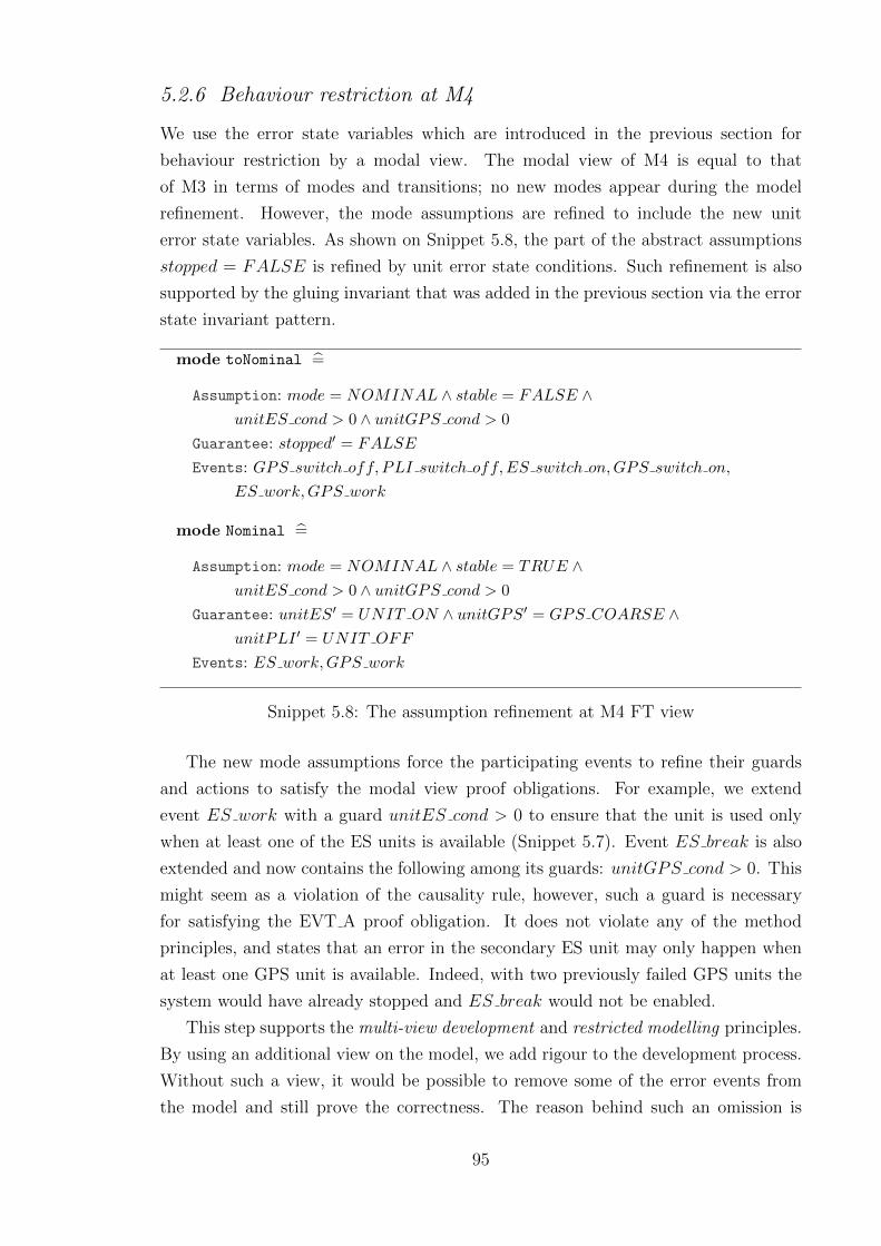
5.2.6 Behaviour restriction at M4

We use the error state variables which are introduced in the previous section for

behaviour restriction by a modal view. The modal view of M4 is equal to that

of M3 in terms of modes and transitions; no new modes appear during the model

refinement. However, the mode assumptions are refined to include the new unit

error state variables. As shown on Snippet 5.8, the part of the abstract assumptions

stopped = FALSE is refined by unit error state conditions. Such refinement is also

supported by the gluing invariant that was added in the previous section via the error

state invariant pattern.

mode toNominal =

Assumption: mode = NOMINAL ∧ stable = FALSE ∧unitES cond > 0 ∧ unitGPS cond > 0

Guarantee: stopped′ = FALSE

Events: GPS switch off, PLI switch off,ES switch on,GPS switch on,

ES work,GPS work

mode Nominal =

Assumption: mode = NOMINAL ∧ stable = TRUE ∧unitES cond > 0 ∧ unitGPS cond > 0

Guarantee: unitES′ = UNIT ON ∧ unitGPS′ = GPS COARSE ∧unitPLI ′ = UNIT OFF

Events: ES work,GPS work

Snippet 5.8: The assumption refinement at M4 FT view

The new mode assumptions force the participating events to refine their guards

and actions to satisfy the modal view proof obligations. For example, we extend

event ES work with a guard unitES cond > 0 to ensure that the unit is used only

when at least one of the ES units is available (Snippet 5.7). Event ES break is also

extended and now contains the following among its guards: unitGPS cond > 0. This

might seem as a violation of the causality rule, however, such a guard is necessary

for satisfying the EVT A proof obligation. It does not violate any of the method

principles, and states that an error in the secondary ES unit may only happen when

at least one GPS unit is available. Indeed, with two previously failed GPS units the

system would have already stopped and ES break would not be enabled.

This step supports the multi-view development and restricted modelling principles.

By using an additional view on the model, we add rigour to the development process.

Without such a view, it would be possible to remove some of the error events from

the model and still prove the correctness. The reason behind such an omission is

95

that the formal method does not guarantee the coverage of error transitions which, in

fact, only contain informal meaning. An additional view focuses attention on abstract

errors and system modal behaviour, and formally ensures that the model implements

the former.

5.3 Conclusions

Prior to modelling the AOCS system, we conducted a refinement planning activity

and identified the refinement steps for this particular system. The steps followed

the refinement strategy proposed in Chapter 4, and were adequate for the AOCS

requirements. During modelling, we have used all the modelling patterns for building

a reactive system, and one of the view templates of the method. Namely, we used

• the safe stop pattern from Section 4.4.1 at M1,

• the error state variable and invariant patterns from Section 4.5.1 and Sec-

tion 4.5.2 correspondingly at M4,

• the fault tolerant behaviour pattern from Section 4.5.3 at M4,

• the behaviour restriction pattern from Section 4.6.1 at M4,

• the behaviour split template from Section 4.5.4 at M3.

The patterns and the refinement strategy are derived by applying the method

principles. Thus, we argue that the refinement strategy is adequate for reactive system

modelling, is supported by a set of patterns, and can be used for creating verified

models of fault tolerant systems.

The AOCS development includes a number of modal views where we explicitly

defined the system modal behaviour from both the functional and fault tolerance

perspectives. Therefore, the method supports explicit modelling of fault tolerance as

a specific case of modal specifications.

By following the top-down strategy of the method, we arrived at a model of the

AOCS system which meets both functional and fault tolerance requirements. The

behaviour restriction step ensures that the functional behaviour and properties can

be modelled in full prior to introducing the environmental restrictions which is shown

at steps M0, M2 and M3. Thus, the method maintains the applicability of the formal

method to modelling the functionality. It advocates and facilitates early modelling of

fault tolerance which is smoothly integrated with functional behaviour.

The method provides facilities for top-down specification of fault tolerant systems

in a form of a set of principles, a refinement strategy which is supported by patterns,

and an additional modal and fault tolerance viewpoint on the system. As shown

96

throughout the evaluation chapter, these facilities can be effectively used to correctly

design fault tolerant systems in a refinement-based formal method.

97

Chapter 6. Conclusions

This section summarises the contributions of the thesis, discusses the strengths and

weaknesses of the proposed method, and shows some of the possible directions of

future research.

6.1 Discussions and Directions of Further Research

The principles and modelling solutions of the proposed method are based on a num-

ber of assumptions. One of the assumptions is the availability of requirements for

the system prior to modelling (see Section 4.1). The proposed method supports a

top-down development process, and we expect to have a requirements document in

order to proceed with the modelling. However, the current engineering practices are

mostly iterative; many significant parts of requirements cannot be initially given with

enough details and are refined during development. This is especially true for such

aspects of systems as dependability and, in particular, fault tolerance. In order to es-

timate reliability and other dependability properties and, thus, define fault tolerance

requirements, one needs to obtain a specification and at least a high-level design of a

system. This implies that the proposed method shall be used iteratively in conjunction

with other currently used model-based design approaches (UML, AADL), reliability

analysis techniques (FMEA, FTA), and traditional software development steps (pro-

totyping, testing). Generally, iterative process requires additional re-modelling efforts

associated with the changes in requirements. This holds for the proposed method as

well; the step-wise process of formal refinement used in the method can only pre-

serve modelling and proof efforts associated with unchanged levels of abstraction. For

example, changes in low-level behaviour of the system will require re-modelling at

low levels of abstraction whereas abstract models would be preserved. In such cases,

the correctness of abstract refinement steps is maintained without extra efforts, and

the assumption about the defined requirements is guaranteed to hold at those steps.

A truly top-down application of the method may only be realised in the context of

verifying an existing design, i.e. produced using traditional (iterative or top-down)

methods for which requirements at this stage are fully defined.

Further issue related to the definition of assumptions is a classical notion of a model

98

adequacy and abstraction of environment. As stated in the principle of environment

modelling in Section 4.1.4, a model must contain an adequate representation of the

system environment. However, the continuous, real-time and stochastic aspects of

many systems may have a significant impact on the modelling and verification process

as it is not always possible to define an adequate discrete state-based abstraction

of the underlying phenomena. Thus, the proposed method is limited to modelling

and verification of those properties and behaviours for which adequate state-based

abstractions can be defined. In the context of fault tolerance modelling, this means

that important properties of many fault tolerance mechanisms cannot be verified

using the proposed method and, more generally, using non-stochastic state-based

formal methods. For example, the essential property of N-modular redundancy, i.e.

the reduced failure rate of the system, cannot be captured in the method. The

model would necessarily contain a discrete form of such a technique. At the level of

abstraction supported by the method the system with and the system without NMR

would be equivalent from the fault tolerance perspective [TTL09].

We envision a number of possible extensions of the method that could widen

its applicability. One possible extension of the approach is to use formalisms with

stochastic choice semantics [HT10; Bal01] as opposed to the currently used demonic

choice semantics. This would allow developers to express rich fault tolerance prop-

erties that involve failure rates and other probabilistic estimations. These can be

based on fault assumptions derived directly from reliability analysis techniques. For

example, fault trees could be used for deriving formal relationship between subsequent

levels of abstraction when applying the error state invariant pattern.

Currently, the method focuses on modelling the system behaviour in reactive style

and postpones sequential decomposition. This ensures expressiveness of safety prop-

erties. We regard using the Use Case (Flow) language [Ili11; Ili12] as a potentially

promising direction of work for verifying local properties carried through sequences

of steps. This could add flexibility to the method in expressing sequential behaviour

and introduce additional type of views bringing benefits associated with multi-view

development.

At the architectural level, the method supports architectural structuring during

functional refinement. Such a structuring could be also derived from an architectural

description described in an existing well-established architecture description language

such as AADL [AADL] and Wright [All97], or in a model-based design language such

as UML [JBR99] and SysML [Gro].

The second part of the method that focuses on control system modelling intro-

duces implementation-level constructs such as a control loop and explicit hardware

read/write operations (see Section 4.8). Models containing these low-level constructs

can be used to obtain verified code using existing code generators such as [EB; MS11].

99

The mentioned solutions could make a strong link between the proposed method and

existing engineering tools and constitute a complete development process.

An important aspect of the proposed development method is the reuse mechanism.

It is currently based on generic modelling patterns that are domain-independent (see

Section 4.9). We envision two possible directions of improvement in this area. The first

solution targets at facilitating reuse within a particular domain. The generic patterns

could be used to instantiate formal models from those expressed in domain-specific

languages (DSL). The main purpose for such an instantiation would be verification,

and the main system design could be done using a DSL.

The second solution is domain-independent and could provide an additional benefit

of proof reuse. A formal technique that can improve reuse of modelling decisions and

proofs can be based on generalisation and further instantiation of parts or complete

models. For example, the airlock case study can be generalised to an N-door “airlock”

representing an access control system. The system would provide access to N actors

according to the (externally) defined rules. Possible instantiations of such a system

could follow rules for a single reader / single writer access, mutual exclusion, or for

N out of M accessors. We believe that such an approach would be particularly useful

during the architectural development process where architects typically seek for and

use existing solutions in the form of patterns. However, the effort required for proofs

in such an approach might be bigger than that for domain-specific models; this is due

to the generality of models and properties being verified.

The proposed method is a top-down development method that is applicable to a

wide range of problem domains. It is especially beneficial for modelling systems with

a single source of control such as embedded systems. The method does not provide

means for model decomposition which is necessary when modelling distributed sys-

tems, business applications, and communication protocols. Such systems are typically

composed of communicating subsystems with distributed logic. In these domains, the

method can be applied at the system and subsystem levels separately. To formally

connect the two levels one can use existing decomposition techniques such as shared

variables, shared events, or modularisation for Event-B [Hoa+11].

6.2 Summary and Contributions

This thesis proposes a development method for formal modelling of fault tolerant sys-

tems. The method focuses on top-down modelling of abstract fault tolerant behaviour

with the purpose of verifying fault tolerance requirements.

The method provides modelling guidelines for building fault tolerant systems. The

guidelines consist of three constituents:

• Modelling principles postulate rules which must be obeyed during modelling

100

• Refinement strategy specifies a sequence of refinement steps for arriving at a

correct model

• Modelling patterns support specific refinement steps and provide a reuse mech-

anism for building fault tolerant systems

The method allows developers to further refine an abstract fault tolerant system

into a control system.

We demonstrate the applicability of the method by instantiating patterns and

templates in Event-B and modelling two medium-scale case studies. The thesis con-

tributes to the following areas:

Adoption of formal methods

The proposed development method and its contributions mentioned above further the

adoption of formal methods. The method provides formal developers with a set of

modelling guidelines that cover three levels of application. The modelling principles

facilitate general understanding of using refinement-based formal methods with inter-

leaving semantics for modelling faults and fault tolerance. The refinement strategy

introduces a well-defined sequence of steps that need to be performed to arrive at a

meaningful model. The modelling patterns and the modal view templates support

engineers with generic modelling solutions and represent a reuse mechanism.

Modelling fault tolerance for systems dependability

The method facilitates modelling fault tolerance formally from the early stages of de-

velopment. Critical systems typically employ fault tolerance as an indistinguishable

part of their behaviour. The early consideration of fault tolerance in refinement-based

methods reduces the modelling efforts, and helps to ensure the overall dependability

of such systems.

Multi-view development

The method includes additional views on the models that capture fault tolerance and

modal features of the systems. The modal viewpoint adds rigour to the formal devel-

opment process through additional proof obligations. It also contributes to readability

of formal models by engineers. The views shorten the gap between requirements and

formal models by allowing modal and fault tolerance requirements to be expressed

diagrammatically.

Rigorous development

The necessity of having formal consistency between views and models brings extra

proof efforts. According to our estimations, application of modal views doubles the

101

proof efforts for both case studies described in this work. The proving process gives

assurance in system behaviour, therefore, the approach adds rigour to the develop-

ment process.

Tool support

The method is tool supported. The modal viewpoint is implemented as a plug-in

for the Rodin environment which includes a diagram editor and a smooth integration

with prover facilities [WIFT]. The patterns of the method can be reused for a par-

ticular domain or application by using the Transformation Patterns plug-in [WIPT].

The patterns plug-in provides facilities for writing model transformations in a sim-

ple object-oriented language, and executing them on demand. Tool support further

facilitates the adoption of the approach and formal methods for building highly de-

pendable systems.

102

References

[AA99] National Aeronautics and Space Administration. Mars Climate Orbiter

Mishap Investigation Report. 1999. url: ftp://ftp.hq.nasa.gov/pub/

pao/reports/2000/MCO_MIB_Report.pdf.

[AADL] Society of Automotive Engineers. Architecture Analysis and Design Lan-

guage (AADL) AS-5506A. 2009.

[Abr10] J.-R. Abrial. Modeling in Event-B - System and Software Engineering.

Cambridge University Press, 2010. isbn: 978-0-521-89556-9.

[Abr96] J.-R. Abrial. The B-Book: Assigning Programs to Meanings. Cambridge

University Press, 1996. isbn: 0-521-49619-5.

[Ace+07] L. Aceto, A. Ingolfsdottir, K. G. Larsen, and J. Srba. Reactive Systems:

Modelling, Specification and Verification. Cambridge University Press,

2007. isbn: 0-521-87546-3.

[Age96] European Space Agency. Ariane 501 Inquiry Board Report. 1996. url:

http://esamultimedia.esa.int/docs/esa-x-1819eng.pdf.

[AKS01] P. Alexander, C. Kong, and D. Schonberger. “A Practical Semantics for

Design Facet Interaction”. In: Proceedings of the 8th IEEE International

Conference and Workshop on Engineering of Computer Based Systems

(ECBS’01). 2001, pp. 229 –236.

[All97] R. J. Allen. “A Formal Approach to Software Architecture”. PhD thesis.

Pittsburgh, PA, USA, 1997. isbn: 0-591-64744-3.

[Alt] The Altarica language. url: https://altarica.labri.fr/forge.

[Amb04] S.W. Ambler. The Object Primer: Agile Modeling-Driven Development

with UML 2.0. Cambridge University Press, 2004. isbn: 978-0-521-54018-

6.

[ASAA09] I. Ait-Sadoune and Y. Ait-Ameur. “A Proof Based Approach for Mod-

elling and Verifying Web Services Compositions”. In: Proceedings of the

2009 14th IEEE International Conference on Engineering of Complex

Computer Systems. ICECCS ’09. IEEE Computer Society, 2009, pp. 1–

10. isbn: 978-0-7695-3702-3.

103

[ATB] Atelier B, the Industrial Tool to Efficiently Deploy the B Method. url:

http://www.atelierb.eu.

[Avi+04] A. Avizienis, J.-C. Laprie, B. Randell, and C. Landwehr. “Basic Concepts

and Taxonomy of Dependable and Secure Computing”. IEEE Transac-

tions on Dependable and Secure Computing 1.1 (Jan. 2004), pp. 11–33.

issn: 1545-5971.

[Avi85] A. Avizienis. “The N-Version Approach to Fault-Tolerant Software”. IEEE

Transactions on Software Engineering SE-11.12 (Dec. 1985), pp. 1491–

1501. issn: 0098-5589. doi: 10.1109/TSE.1985.231893.

[Avr+96] D. Avresky, J. Arlat, J.-C. Laprie, and Y. Crouzet. “Fault injection for

formal testing of fault tolerance”. IEEE Transactions on Reliability 45.3

(Sept. 1996), pp. 443–455. issn: 0018-9529. doi: 10.1109/24.537015.

[BA05] F. Badeau and A. Amelot. “Using B as a High Level Programming Lan-

guage in an Industrial Project: Roissy VAL”. In: Proceedings of the 4th

International Conference on Formal Specification and Development in Z

and B. ZB’05. Guildford, UK: Springer-Verlag, 2005, pp. 334–354. isbn:

978-3-540-25559-8.

[Bac80] R. J. R. Back. Correctness Preserving Program Refinements: Proof The-

ory and Applications. Mathematical Centre tracts. Mathematisch Cen-

trum, 1980. isbn: 978-9-061-96207-6.

[Bal01] G. Balbo. “Introduction to Stochastic Petri Nets”. In: Lectures on For-

mal Methods and PerformanceAnalysis. Ed. by Ed Brinksma, Holger Her-

manns, and Joost-Pieter Katoen. Vol. 2090. Lecture Notes in Computer

Science. Springer Berlin Heidelberg, 2001, pp. 84–155. isbn: 978-3-540-

42479-6.

[Bec03] K. Beck. Test-Driven Development by Example. The Addison-Wesley Sig-

nature Series. Addison-Wesley, 2003. isbn: 978-0321146533.

[Beh+99] P. Behm, P. Benoit, A. Faivre, and J.-M. Meynadier. “Meteor: A Suc-

cessful Application of B in a Large Project”. In: Proceedings of the World

Congress on Formal Methods in the Development of Computing Systems

FM’99. Vol. 1708. Lecture Notes in Computer Science. Springer Berlin /

Heidelberg, 1999, pp. 712–712. isbn: 978-3-540-66587-8.

[BH06] J. P. Bowen and M. G. Hinchey. “Ten Commandments of Formal Meth-

ods ...Ten Years Later”. IEEE Computer 39.1 (Jan. 2006), pp. 40–48.

104

[Bie+04] P. Bieber, C. Bougnol, C. Castel, J.-P. Heckmann, C. Kehren, S. Metge,

C. Seguin, and C. Seguin. “Safety Assessment with Altarica - Lessons

Learnt Based on Two Aircraft System Studies”. In: 18th IFIP World

Computer Congress, Topical Day on New Methods for Avionics Certifi-

cation. 2004, p. 26.

[BR85] S.D. Brookes and A.W. Roscoe. “An improved failures model for com-

municating processes”. In: Seminar on Concurrency. Ed. by StephenD.

Brookes, AndrewWilliam Roscoe, and Glynn Winskel. Vol. 197. Lecture

Notes in Computer Science. Springer Berlin Heidelberg, 1985, pp. 281–

305. isbn: 978-3-540-15670-3. doi: 10.1007/3-540-15670-4_14. url:

http://dx.doi.org/10.1007/3-540-15670-4_14.

[Bro+05] M. Broy, B. Jonsson, J.-P. Katoen, M. Leucker, and A. Pretschner. Model-

Based Testing of Reactive Systems: Advanced Lectures (Lecture Notes in

Computer Science). Springer-Verlag New York, 2005. isbn: 3-540-26278-

4.

[Bry11] J. W. Bryans. “Developing a Consensus Algorithm using Stepwise Refine-

ment”. In: Proceedings of the 13th International Conference on Formal

Methods and Software Engineering. ICFEM’11. Durham, UK: Springer-

Verlag, 2011, pp. 553–568. isbn: 978-3-642-24558-9.

[BS03] E. Borger and R. F. Stark. Abstract State Machines. A Method for High-

Level System Design and Analysis. Springer, 2003. isbn: 978-3-540-00702-

9.

[BS89] R.-J. Back and K. Sere. “Stepwise Refinement of Action Systems”. In:

Proceedings of the International Conference on Mathematics of Program

Construction, 375th Anniversary of the Groningen University. London,

UK: Springer-Verlag, 1989, pp. 115–138. isbn: 3-540-51305-1.

[But12] M. Butler. Towards a Cookbook for Modelling and Refinement of Control

Problems. Working paper, unpublished. 2012. url: http://deploy-

eprints.ecs.soton.ac.uk/108/.

[BV07] M. Bozzano and A. Villafiorita. “The FSAP/NuSMV-SA Safety Anal-

ysis Platform”. International Journal on Software Tools for Technology

Transfer 9.1 (Feb. 2007), pp. 5–24. issn: 1433-2779.

[CDV98] J. Crow and B. Di Vito. “Formalizing Space Shuttle Software Require-

ments: Four Case Studies”. ACM Transactions on Software Engineering

and Methodology 7.3 (July 1998), pp. 296–332. issn: 1049-331X.

105

[Cha+06] P. Chalin, J. Kiniry, G. Leavens, and E. Poll. “Beyond Assertions: Ad-

vanced Specification and Verification with JML and ESC/Java2”. In: Pro-

ceedings of the 4th International Conference on Formal Methods for Com-

ponents and Objects. FMCO’05. Amsterdam, The Netherlands: Springer-

Verlag, 2006, pp. 342–363. isbn: 978-3-540-36749-9.

[Cla08] E. M. Clarke. “25 Years of Model Checking”. In: ed. by O. Grumberg

and H. Veith. Vol. 5000. Lecture Notes in Computer Science. Berlin,

Heidelberg: Springer-Verlag, 2008. Chap. The Birth of Model Checking,

pp. 1–26. isbn: 978-3-540-69849-4.

[D1.1] F. Loesch, R. Gmehlich, K. Grau, M. Mazzara, and C. Jones. DEPLOY

Deliverable D1.1: Report on Pilot Deployment in Automotive Sector. Jan.

2010. url: http : / / www . deploy - project . eu / pdf / D19 - pilot -

deployment-in-the-automotive-sector.pdf.

[D15.5] T. Lecomte, A. Romanovsky, M. Butler, and E. Troubitsyna. DEPLOY

Deliverable D15.5: Final Dissemination / Exploitation Report. Apr. 2012.

url: http://www.deploy-project.eu/pdf/D52.pdf.

[D2.1] J. Falampin. DEPLOY Deliverable D2.1: Report on Pilot Deployment in

Transportation Sector. Sept. 2009. url: http://www.deploy-project.

eu/pdf/d16_final6.pdf.

[D3.1] D. Ilic, T. Latvala, P. Vaisanen, K. Varpaaniemi, L. Laibinis, and E.

Troubitsyna. DEPLOY Deliverable D3.1: Report on Pilot Deployment in

Space Sector. Jan. 2010. url: http://www.deploy-project.eu/pdf/

D20-pilot-deployment-in-the-space-sector-final-version.pdf.

[D4.1] A. Roth, V. Kozyura, W. Wei, S. Wieczorek, A. Furst, T.S. Hoang, and J.

Bryans. DEPLOY Deliverable D4.1: Report on Pilot Deployment in Busi-

ness Information Sector. Jan. 2010. url: http://www.deploy-project.

eu/pdf/D21-pilot-deployment-in-business-information-software(4)

.pdf.

[DEP] FP7 DEPLOY Project: Industrial deployment of system engineering meth-

ods providing high dependability and productivity. 2008. url: http://

www.deploy-project.eu/.

[Dot+09] F. L. Dotti, A. Iliasov, L. Ribeiro, and A. Romanovsky. “Modal Sys-

tems: Specification, Refinement and Realisation”. In: Proceedings of the

11th International Conference on Formal Engineering Methods: Formal

Methods and Software Engineering. ICFEM ’09. Rio de Janeiro, Brazil:

Springer-Verlag, 2009, pp. 601–619. isbn: 978-3-642-10372-8.

106

[DR+10] D. Di Ruscio, I. Malavolta, H. Muccini, P. Pelliccione, and A. Pieranto-

nio. “Developing Next Generation ADLs through MDE Techniques”. In:

Proceedings of the 32nd ACM/IEEE International Conference on Soft-

ware Engineering - Volume 1. ICSE ’10. Cape Town, South Africa: ACM,

2010, pp. 85–94. isbn: 978-1-60558-719-6.

[DW06] J. Derrick and H. Wehrheim. “Model transformations incorporating mul-

tiple views”. In: Proceedings of the 11th international conference on Al-

gebraic Methodology and Software Technology. AMAST’06. Kuressaare,

Estonia: Springer-Verlag, 2006, pp. 111–126. isbn: 3-540-35633-9, 978-3-

540-35633-2.

[Eas+98] S. Easterbrook, R. Lutz, R. Covington, J. Kelly, Y. Ampo, and D. Hamil-

ton. “Experiences using Lightweight Formal Methods for Requirements

Modeling”. IEEE Transactions on Software Engineering 24.1 (Jan. 1998),

pp. 4 –14. issn: 0098-5589.

[EB] EB2ALL - The Event-B to C, C++, Java and C# Code Generator. url:

http://eb2all.loria.fr/.

[ECL] Eclipse open platform for building development environments. url: http:

//www.eclipse.org/.

[FBR12] A. S. Fathabadi, M. Butler, and A. Rezazadeh. “A Systematic Approach

to Atomicity Decomposition in Event-B”. In: Proceedings of the 10th

International Conference on Software Engineering and Formal Methods

SEFM’12. Thessaloniki, Greece, Oct. 2012.

[Fit+10] J. Fitzgerald, P. G. Larsen, K. Pierce, M. Verhoef, and S. Wolff. “Collab-

orative Modelling and Co-Simulation in the Development of Dependable

Embedded Systems”. In: Proceedings of the 8th International Conference

on Integrated Formal Methods. IFM’10. Nancy, France: Springer-Verlag,

2010, pp. 12–26. isbn: 3-642-16264-9, 978-3-642-16264-0.

[FKG90] A. Finkelstein, J. Kramer, and M. Goedicke. “ViewPoint Oriented Soft-

ware Development”. In: Proceedings of the 3rd International Workshop

on Software Engineering and its Applications. Toulouse, France: Actes,

Dec. 1990. isbn: 9782906899490.

[FM92] P. Fenelon and J. A. Mcdermid. New Directions in Software Safety:

Causal Modelling as an Aid to Integration. Technical report, Department

of Computer Science, University of York, UK. 1992.

[FMIC] Info Centre for FMEA. url: http://www.fmeainfocentre.com.

107

[FMTR] IEC 60812. Functional safety of electrical/electronical/programmable elec-

tronic safety-related systems, analysis techniques for system reliability -

procedure for failure mode and effect analysis (FMEA). Technical report,

International Electrotechnical Commission IEC. 1991.

[For04] U.S.-Canada Power System Outage Task Force. Final Report on the Au-

gust 14th Blackout in the United States and Canada. 2004. url: https:

//reports.energy.gov.

[Gam+94] E. Gamma, R. Helm, R. Johnson, and J. Vlissides. Design Patterns:

Elements of Reusable Object-Oriented Software. 1st ed. Addison-Wesley

Professional, Nov. 1994. isbn: 0201633612.

[GIL12] G. Grov, A. Ireland, and M. T. Llano. “Refinement Plans for Informed

Formal Design”. In: Proceedings of the 3rd international conference on

Abstract State Machines, Alloy, B, VDM, and Z. Ed. by S. Gnesi S.

Khurshid M. Leuschel S. Reeves J. Derrick J. Fitzgerald and E. Ric-

cobene. Vol. 7316. ABZ’12. Pisa, Italy: Springer-Verlag, 2012, pp. 208–

222. isbn: 978-3-642-30884-0.

[GO11] A. O. Gomes and M. V. M. Oliveira. “Formal Development of a Car-

diac Pacemaker: from Specification to Code”. In: Proceedings of the 13th

Brazilian Conference on Formal Methods: Foundations and Applications.

SBMF’10. Natal, Brazil: Springer-Verlag, 2011, pp. 210–225. isbn: 978-

3-642-19828-1.

[Goe+00] M. Goedicke, B. Enders, T. Meyer, and G. Taentzer. “ViewPoint-Oriented

Software Development: Tool Support for Integrating Multiple Perspec-

tives by Distributed Graph Transformation”. English. In: Tools and Al-

gorithms for the Construction and Analysis of Systems. Ed. by S. Graf

and M. Schwartzbach. Vol. 1785. Lecture Notes in Computer Science.

Springer Berlin Heidelberg, 2000, pp. 43–47. isbn: 978-3-540-67282-1.

[Gro] Object Modelling Group. The official OMG SysML site. url: http :

//www.omgsysml.org/.

[Ham+95] D. Hamilton, R. Covington, J. Kelly, C. Kirkwood, M. Thomas, A. R.

Flora-Holmquist, M. G. Staskauskas, S. P. Miller, M. Srivas, G. Cle-

land, and D. MacKenzie. “Experiences in Applying Formal Methods to

the Analysis of Software and System Requirements”. In: Proceedings of

the 1st Workshop on Industrial-Strength Formal Specification Techniques.

WIFT ’95. Washington, DC, USA: IEEE Computer Society, 1995, pp. 30–

43. isbn: 0-8186-7005-3.

108

[HB95] M.G. Hinchey and J.P. Bowen. Applications of Formal Methods. Prentice-

Hall International Series in Computer Science. Prentice Hall, 1995. isbn:

978-0-133-66949-7.

[HB99] M. G. Hinchey and J. P. Bowen. High-Integrity System Specification and

Design. Ed. by S. A. Schuman. 1st. Springer-Verlag New York, Inc., 1999.

isbn: 3540762264.

[HBH08] R. M. Hierons, J. P. Bowen, and M. Harman, eds. Formal Methods and

Testing, An Outcome of the FORTEST Network, Revised Selected Papers.

Vol. 4949. Lecture Notes in Computer Science. Springer, 2008. isbn: 978-

3-540-78916-1.

[HBV10] M. Hinchey, J. P. Bowen, and E. Vassev. “Formal Methods”. In: Encyclo-

pedia of Software Engineering. Ed. by P. A. Laplante. Taylor & Francis,

2010, pp. 308–320. isbn: 978-1-4200-5977-9.

[HG93] C. Hennebert and G. Guiho. “SACEM: A Fault Tolerant System for Train

Speed Control”. In: Proceedings of the 23rd International Symposium on

Fault-Tolerant Computing FTCS-23. IEEE Computer Society, June 1993,

pp. 624–628.

[HH11] T. S. Hoang and S. Hudon. Developing Control Systems with Some Fragile

Environment. Technical Report 723 Department of Computer Science,

ETH-Zurich, Switzerland. Apr. 2011.

[HJJ03] I. J. Hayes, M. A. Jackson, and C. B. Jones. “Determining the Specifica-

tion of a Control System from that of its Environment”. In: Proceedings

of the International Symposium of Formal Methods Europe FME’03. Ed.

by K. Araki, S. Gnesi, and D. Mandrioli. Vol. 2805. Lecture Notes in

Computer Science. Pisa, Italy: Springer, Sept. 2003, pp. 154–169.

[HLV11] M. Hecht, A. Lam, and C. Vogl. “A Tool Set for Integrated Software

and Hardware Dependability Analysis using the Architecture Analysis

and Design Language (AADL) and Error Model Annex”. In: Proceedings

of the 16th IEEE International Conference on Engineering of Complex

Computer Systems ICECCS’11. Apr. 2011, pp. 361 –366. isbn: 978-1-

61284-853-2.

[Hoa+11] T. S. Hoang, A. Iliasov, R. Silva, and W. Wei. “A Survey on Event-B

Decomposition”. Electronic Communications of the EASST 46 (2011).

issn: 1863-2122.

109

[HS99] M. Heisel and J. Souquieres. “A Method for Requirements Elicitation

and Formal Specification”. In: Proceedings of the 18th International Con-

ference on Conceptual Modeling ER’99. Ed. by Jacky Akoka, Mokrane

Bouzeghoub, Isabelle Comyn-Wattiau, and Elisabeth Metais. Vol. 1728.

Lecture Notes in Computer Science. Springer Berlin / Heidelberg, 1999,

pp. 767–767. isbn: 978-3-540-66686-8.

[HT10] O. Hasan and S. Tahar. “Formal Probabilistic Analysis: A Higher-Order

Logic Based Approach”. In: Abstract State Machines, Alloy, B and Z.

Ed. by Marc Frappier, Uwe Glsser, Sarfraz Khurshid, Rgine Laleau, and

Steve Reeves. Vol. 5977. Lecture Notes in Computer Science. Springer

Berlin Heidelberg, 2010, pp. 2–19. isbn: 978-3-642-11810-4.

[Hun89] W. A. Hunt. “Microprocessor Design Verification”. Journal of Automated

Reasoning 5 (1989), pp. 429–460.

[Ili+10] A. Iliasov, E. Troubitsyna, L. Laibinis, A. Romanovsky, K. Varpaaniemi,

D. Ilic, and T. Latvala. “Developing Mode-Rich Satellite Software by

Refinement in Event B”. In: Proceedings of the 15th International Con-

ference on Formal Methods for Industrial Critical Systems. FMICS’10.

Antwerp, Belgium: Springer-Verlag, 2010, pp. 50–66. isbn: 3-642-15897-

8, 978-3-642-15897-1.

[Ili11] A. Iliasov. “Use Case Scenarios as Verification Conditions: Event-B/Flow

Approach”. In: Proceedings of the 3rd International Conference on Soft-

ware Engineering for Resilient Systems. SERENE’11. Geneva, Switzer-

land: Springer-Verlag, 2011, pp. 9–23. isbn: 978-3-642-24123-9.

[Ili12] A. Iliasov. “Augmenting Formal Development with Use Case Reason-

ing”. In: Proceedings of the 17th Ada-Europe International Conference

on Reliable Software Technologies. Ed. by Mats Brorsson and LuisMiguel

Pinho. Vol. 7308. Lecture Notes in Computer Science. Stockholm, Swe-

den: Springer Berlin Heidelberg, June 2012, pp. 133–146. isbn: 978-3-

642-30597-9.

[Int06] ECMA International. Standard ECMA-367 - Eiffel: Analysis, Design and

Programming Language 2nd edition. June 2006. url: http://www.ecma-

international.org/publications/standards/Ecma-367.htm.

[IRD09] A. Iliasov, A. Romanovsky, and F. L. Dotti. “Structuring Specifications

with Modes”. In: Proceedings of the Latin-American Symposium on De-

pendable Computing, LADC’09. Vol. 0. Los Alamitos, CA, USA: IEEE

Computer Society, 2009, pp. 81–88. isbn: 978-0-7695-3760-3.

110

[Jac01] M. Jackson. Problem Frames: Analyzing and Structuring Software De-

velopment Problems. Boston, MA, USA: Addison-Wesley Longman Pub-

lishing Co., Inc., 2001. isbn: 0-201-59627-X.

[Jac95] D. Jackson. “Structuring Z Specifications with Views”. ACM Transac-

tions on Software Engineering and Methodology 4.4 (Oct. 1995), pp. 365–

389. issn: 1049-331X.

[Jal89] P. Jalote. “Fault Tolerant Processes”. Distributed Computing 3.4 (1989),

pp. 187–195. issn: 0178-2770. doi: 10.1007/BF01784887.

[JBR99] I. Jacobson, G. Booch, and J. E. Rumbaugh. The Unified Software De-

velopment Process - the Complete Guide to the Unified Process from the

Original Designers. Addison-Wesley object technology series. Addison-

Wesley, 1999, pp. I–XXIX, 1–463. isbn: 978-0-201-57169-1.

[Jef+09] R.D. Jeffords, C.L. Heitmeyer, M. Archer, and E.I. Leonard. “A Formal

Method for Developing Provably Correct Fault-Tolerant Systems Using

Partial Refinement and Composition”. In: FM. 2009, pp. 173–189.

[JH07] A. Joshi and M. P. E. Heimdahl. “Behavioral Fault Modeling for Model-

based Safety Analysis”. In: Proceedings of the 10th IEEE High Assur-

ance Systems Engineering Symposium. HASE ’07. Washington, DC, USA:

IEEE Computer Society, 2007, pp. 199–208. isbn: 0-7695-3043-5.

[JHL11] M. Jastram, S. Hallerstede, and L. Ladenberger. “Mixing Formal and

Informal Model Elements for Tracing Requirements”. Electronic Com-

munications of the EASST 46 (2011). issn: 1863-2122.

[JM94] F. Jahanian and A. K. Mok. “Modechart: A Specification Language for

Real-Time Systems”. IEEE Transactions on Software Engineering 20 (12

Dec. 1994), pp. 933–947. issn: 0098-5589.

[Jon90] C. B. Jones. Systematic Software Development using VDM (2nd ed.) Up-

per Saddle River, NJ, USA: Prentice-Hall, Inc., 1990. isbn: 0-13-880733-

7.

[KA03] C. Kong and P. Alexander. “The Rosetta Meta-Model Framework”. In:

Los Alamitos, CA, USA: IEEE Computer Society, Apr. 2003, pp. 133–

140. isbn: 0-7695-1917-2.

[Kni02] J. Knight. “Safety critical systems: challenges and directions”. In: Pro-

ceedings of the 24th International Conference on Software Engineering.

ICSE ’02. Orlando, Florida: ACM, 2002, pp. 547–550. isbn: 1-58113-472-

X. doi: 10.1145/581339.581406. url: http://doi.acm.org/10.1145/

581339.581406.

111

[Kni12] J. Knight. Dependable Computing for Software Engineers. Boca Raton,

US: CRC Press, Taylot & Francis Group, 2012. isbn: 978-1-4398-6255-1.

[LA90] P. A. Lee and T. Anderson. Fault Tolerance: Principles and Practice.

Springer-Verlag New York, Inc., 1990. isbn: 0387820779.

[Lab10] Jet Propulsion Laboratory. Report on the Loss of the Mars Polar Lander

and Deep Space 2 Missions, JPL D-18709. 2010.

[Lam94] L. Lamport. “The temporal logic of actions”. ACM Transactions on Pro-

gramming Languages and Systems (TOPLAS) 16.3 (May 1994), pp. 872–

923. issn: 0164-0925.

[LB08] M. Leuschel and M. Butler. “ProB: an Automated Analysis Toolset for

the B Method”. Software Tools for Technology Transfer 10.2 (Feb. 2008),

pp. 185–203. issn: 1433-2779.

[LGP11] C. Lauer, R. German, and J. Pollmer. “Fault Tree Synthesis from UML

Models for Reliability Analysis at Early Design Stages”. SIGSOFT Soft-

ware Engineering Notes 36.1 (Jan. 2011), pp. 1–8. issn: 0163-5948.

[LIR10] I. Lopatkin, A. Iliasov, and A. Romanovsky. “On Fault Tolerance Reuse

during Refinement”. In: Proceedings of the 2nd International Workshop

on Software Engineering for Resilient Systems, SERENE’10. available as

CS-TR-1188 at Newcastle University, UK. London, UK, Apr. 2010.

[Lop+11] I. Lopatkin, A. Iliasov, A. Romanovsky, Y. Prokhorova, and E. Troubit-

syna. “Patterns for Representing FMEA in Formal Specification of Con-

trol Systems”. In: The 13th IEEE International High Assurance Systems

Engineering Symposium (HASE’11). Boca Raton, FL, USA, Nov. 2011,

pp. 146–151.

[LT04a] L. Laibinis and E. Troubitsyna. “Fault Tolerance in a Layered Architec-

ture: A General Specification Pattern in B”. In: Proceedings of the 2nd

International Conference on Software Engineering and Formal Methods.

SEFM’04. Beijing, China: IEEE Computer Society, Sept. 2004, pp. 346–

355. isbn: 0-7695-2222-X.

[LT04b] L. Laibinis and E. Troubitsyna. “Refinement of Fault Tolerant Control

Systems in B”. In: Proceedings of the 23rd International Conference on

Computer Safety, Reliability, and Security (SAFECOMP’04). Potsdam,

Germany, 2004, pp. 254–268.

[LV62] R. E. Lyons and W. Vanderkulk. “The use of triple-modular redundancy

to improve computer reliability”. IBM Journal of Research and Develop-

ment 6.2 (Apr. 1962), pp. 200–209. issn: 0018-8646.

112

[MAV05] C. Metayer, J.R. Abrial, and L. Voisin, eds. Rodin Deliverable D7: Event-

B Language. Project IST-511599, School of Computing Science, Newcas-

tle University, 2005.

[McK+05] M. L. McKelvin Jr., G. Eirea, C. Pinello, S. Kanajan, and A. L. Sangiovanni-

Vincentelli. “A Formal Approach to Fault Tree Synthesis for the Analysis

of Distributed Fault Tolerant Systems”. In: Proceedings of the 5th ACM

International Conference on Embedded software. EMSOFT ’05. Jersey

City, NJ, USA: ACM, 2005, pp. 237–246. isbn: 1-59593-091-4.

[MR98] F. Maraninchi and Y. Remond. “Mode-Automata: About Modes and

States for Reactive Systems”. In: Proceedings of the 7th European Sym-

posium On Programming ESOP’98. Lecture Notes in Computer Science

1381.7. Lisbon, Portugal: Springer Verlag, 1998. isbn: 9783540643029.

[MS11] D. Mery and N. K. Singh. “Automatic Code Generation from Event-

B Models”. In: Proceedings of the 2nd Symposium on Information and

Communication Technology. SoICT ’11. Hanoi, Vietnam: ACM, 2011,

pp. 179–188. isbn: 978-1-4503-0880-9.

[MSCC] Microsoft Research. Code Contracts: Language and Tool Support. url:

http://research.microsoft.com/en-us/projects/contracts/.

[MSSP] Microsoft Research. Spec#: Formal Language for API Contracts. url:

http://research.microsoft.com/en-us/projects/specsharp/.

[Mur+08] K. Murale, S. Hildebrandt, P. Bojsen, and A. Urzua. “AMD64 Processor

Front-End Verification (at Unit-Level Testbench) with Instruction Set

Simulator”. In: Proceedings of the 2008 Ninth International Workshop on

Microprocessor Test and Verification. MTV’08. Washington, DC, USA:

IEEE Computer Society, 2008, pp. 81–87. isbn: 978-0-7695-3581-4.

[Pap+11] Y. Papadopoulos, M. Walker, D. Parker, E. Rude, R. Hamann, A. Uhlig,

U. Gratz, and R. Lien. “Engineering Failure Analysis and Design Op-

timisation with HiP-HOPS”. Engineering Failure Analysis 18.2 (2011),

pp. 590 –608. issn: 1350-6307.

[Pel09] R. Pelanek. “Fighting State Space Explosion: Review and Evaluation”.

In: Proceedings of the 14th International Workshop on Formal Methods

for Industrial Critical Systems FMICS’09. Berlin, Heidelberg: Springer-

Verlag, 2009, pp. 37–52. isbn: 978-3-642-03239-4.

[Pel91] J. Peleska. “Design and verification of fault tolerant systems with CSP”.

Distributed Computing 5.2 (1991), pp. 95–106. issn: 0178-2770.

113

[PJB99] V. A. Patankar, A. Jain, and R. E. Bryant. “Formal Verification of an

ARM Processor”. In: Proceedings of the 12th International Conference

on VLSI Design - ’VLSI for the Information Appliance’. VLSID ’99.

Washington, DC, USA: IEEE Computer Society, 1999, pp. 282–. isbn:

0-7695-0013-7.

[Pop+01] P. Popov, S. Riddle, A. Romanovsky, and L. Strigini. “On systematic

design of protectors for employing OTS items”. In: Proceedings of the

27th Euromicro Conference. 2001, pp. 22–29. doi: 10.1109/EURMIC.

2001.952434.

[PROB] ProB. Animator and Model Checker for the B Method. url: http://www.

stups.uni-duesseldorf.de/ProB/index.php5/The_ProB_Animator_

and_Model_Checker.

[QNX] QNX Software Systems Limited. Webinar. Lessons Learned: using For-

mal Methods to Develop Medical Device Software. 2012. url: http://

www.qnx.com/news/web_seminars/medical_device_software.html?

elq.

[RL12] A.G. Russo and L. Ladenberger. “A Formal Approach to Safety Verifica-

tion of Railway Signaling Systems”. In: Proceeding of the Reliability and

Maintainability Symposium (RAMS’12). Jan. 2012, pp. 1 –4.

[ROD] The RODIN platform. url: http://rodin- b- sharp.sourceforge.

net/.

[Ros95] D. S. Rosenblum. “A Practical Approach to Programming With Asser-

tions”. IEEE Transactions on Software Engineering 21.1 (Jan. 1995),

pp. 19–31. issn: 0098-5589.

[RSH11] S. Rubini, F. Singhoff, and J. Hugues. “Modeling and Verification of

Memory Architectures with AADL and REAL”. In: Proceedings of the

16th IEEE International Conference on Engineering of Complex Com-

puter Systems ICECCS’11. Apr. 2011, pp. 338 –343.

[Rus89] J. Rushby. “Formal Methods and Critical Systems in the Real World”.

In: Proceedings of Formal Methods for Trustworthy Computer Systems

(FM89). Halifax, Nova Scotia, Canada: Springer-Verlag Workshops in

Computing, July 1989, pp. 121–125.

[RV01] J. A. Robinson and A. Voronkov, eds. Handbook of Automated Reasoning

(in 2 volumes). Elsevier and MIT Press, 2001. isbn: 0-444-50813-9, 0-

262-18223-8.

114

[S1471] ISO/IEC/IEEE. Std 42010:2011, Systems and software engineering - Ar-

chitecture description. Based on IEEE Std 1471:2000, Recommended Prac-

tice for Architectural Description of Software-intensive Systems. 2011.

url: http://www.iso-architecture.org/ieee-1471/.

[SB11] M. R. Sarshogh and M. Butler. “Specification and Refinement of Dis-

crete Timing Properties in Event-B”. In: Proceedings of the 11th Inter-

national Workshop on Automated Verification of Critical Systems AV-

oCS’11. Sept. 2011.

[Sca02] W. Scacchi. “Process Models in Software Engineering”. In: Encyclopedia

of Software Engineering. John Wiley & Sons, Inc., 2002.

[SSF] Space Systems Finland. url: http://www.ssf.fi.

[Sto96] N. R. Storey. Safety Critical Computer Systems. Boston, MA, USA:

Addison-Wesley Longman Publishing Co., Inc., 1996. isbn: 0201427877.

[STS] Siemens Transportation Systems. url: http://www.mobility.siemens.

com/mobility/global/en/pages/siemens-mobility.aspx.

[TTL09] A. Tarasyuk, E. Troubitsyna, and L. Laibinis. Reliability Assessment in

Event-B. TUCS Technical Report No 932, Department of Information

Technologies, Aabo Akademi University, Turku, Finland. 2009.

[Ves81] W.E. Vesely. Fault Tree Handbook. Systems and Reliability Research,

Office of Nuclear Regulatory Research, U.S. Nuclear Regulatory Com-

mission, 1981.

[WD96] J. Woodcock and J. Davies. Using Z: Specification, Refinement, and

Proof. Prentice Hall International Series in Computer Science. Prentice

Hall, 1996. isbn: 9780139484728.

[WIFT] Wiki page for Modal and Fault Tolerance Views language and tool support.

url: http://wiki.event-b.org/index.php/Mode/FT_Views.

[Win94] P. J. Windley. “Specifying Instruction-Set Architectures in HOL: A Primer”.

In: Proceedings of the 7th International Workshop on Higher Order Logic

Theorem Proving and Its Applications. London, UK: Springer-Verlag,

1994, pp. 440–455. isbn: 3-540-58450-1.

[WIPT] Transformation Patterns wiki page. url: http://wiki.event-b.org/

index.php/Transformation_patterns.

[Woo+09] J. Woodcock, P. G. Larsen, J. Bicarregui, and J. S. Fitzgerald. “Formal

Methods: Practice and Experience”. ACM Computing Surveys 41.4 (Oct.

2009), 19:1–19:36. issn: 0360-0300.

115

[Yua+11] F. Yuan, S. Wright, K. Eder, and D. May. “Managing Complexity Through

Abstraction: A Refinement-Based Approach to Formalize Instruction Set

Architectures”. In: Proceedings of the 13th International Conference on

Formal Engineering Methods (ICFEM’11). Lecture Notes in Computer

Science 6991, Oct. 2011, pp. 585–600. isbn: 978-3-642-24558-9.

116

Appendix A: Airlock Case Study Model

This appendix contains full Event-B models for the airlock system used as a case study

throughout Chapter 4. The development produced a total of 417 proof obligations,

356 of which were proven automatically, and 61 required interactive proof. A Rodin

project containing the proved models can be found in the Examples section at [WIFT].

A.1 Context C0

context c0

sets

DOOR STATE

constants

OPENED CLOSED OPENING CLOSING STOPPED

LOW PRESSURE HIGH PRESSURE

axioms

axm1: partition(DOOR STATE, OPENED, CLOSED,OPENING, CLOSING, STOPPED)

axm2: LOW PRESSURE = 0

axm3: HIGH PRESSURE = 2

end

A.2 Machine M0

machine m0 sees c0

variables

door1 door2 pressure

invariants

inv1: door1 ∈ DOOR STATE

inv2: door2 ∈ DOOR STATE

inv3: pressure ∈ N

117

inv4: door1 6= CLOSED⇒ pressure = LOW PRESSURE

inv5: door2 6= CLOSED⇒ pressure = HIGH PRESSURE

inv6: door1 = CLOSED ∨ door2 = CLOSED

inv7: pressure > LOW PRESSURE⇒ door1 = CLOSED

inv8: pressure < HIGH PRESSURE⇒ door2 = CLOSED

inv9: pressure ≥ LOW PRESSURE ∧ pressure ≤ HIGH PRESSURE

events

event INITIALISATION

then

act1: door1 := CLOSED

act2: door2 := CLOSED

act3: pressure := HIGH PRESSURE

end

event open1 =

when

grd1: door1 = CLOSED ∨ door1 = STOPPED

grd2: pressure = LOW PRESSURE

grd3: door2 = CLOSED

then

act1: door1 := OPENING

end

event opened1 =

when

grd1: door1 = OPENING

then

act1: door1 := OPENED

end

event close1 =

when

grd1: door1 = OPENED ∨ door1 = STOPPED

then

act1: door1 := CLOSING

end

event closed1 =

when

grd1: door1 = CLOSING

then

act1: door1 := CLOSED

end

118

event open2 =

when

grd1: door2 = CLOSED ∨ door2 = STOPPED

grd2: pressure = HIGH PRESSURE

grd3: door1 = CLOSED

then

act1: door2 := OPENING

end

event opened2 =

when

grd1: door2 = OPENING

then

act1: door2 := OPENED

end

event close2 =

when

grd1: door2 = OPENED ∨ door2 = STOPPED

then

act1: door2 := CLOSING

end

event closed2 =

when

grd1: door2 = CLOSING

then

act1: door2 := CLOSED

end

event pump up =

when

grd1: door1 = CLOSED ∧ door2 = CLOSED

grd2: pressure < HIGH PRESSURE

then

act1: pressure := pressure+ 1

end

event pump down =

when

grd1: door1 = CLOSED ∧ door2 = CLOSED

grd2: pressure > LOW PRESSURE

then

act1: pressure := pressure− 1

119

end

event stop1 =

when

grd1: door1 = OPENING ∨ door1 = CLOSING

then

act1: door1 := STOPPED

end

event stop2 =

when

grd1: door2 = OPENING ∨ door2 = CLOSING

then

act1: door2 := STOPPED

end

end

A.3 Machine M1

machine m1 refines m0 sees c0

variables

door1 door2 pressure stopped

invariants

inv1: stopped ∈ BOOL

events

event INITIALISATION

extended

then

act1: door1 := CLOSED

act2: door2 := CLOSED

act3: pressure := HIGH PRESSURE

act4: stopped := FALSE

end

event open1 = extends open1

when

grd1: door1 = CLOSED ∨ door1 = STOPPED

grd2: pressure = LOW PRESSURE

grd3: door2 = CLOSED

grd stopped: stopped = FALSE

120

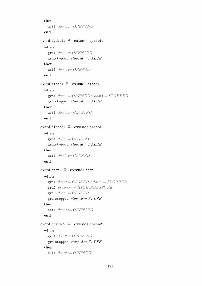
then

act1: door1 := OPENING

end

event opened1 = extends opened1

when

grd1: door1 = OPENING

grd stopped: stopped = FALSE

then

act1: door1 := OPENED

end

event close1 = extends close1

when

grd1: door1 = OPENED ∨ door1 = STOPPED

grd stopped: stopped = FALSE

then

act1: door1 := CLOSING

end

event closed1 = extends closed1

when

grd1: door1 = CLOSING

grd stopped: stopped = FALSE

then

act1: door1 := CLOSED

end

event open2 = extends open2

when

grd1: door2 = CLOSED ∨ door2 = STOPPED

grd2: pressure = HIGH PRESSURE

grd3: door1 = CLOSED

grd stopped: stopped = FALSE

then

act1: door2 := OPENING

end

event opened2 = extends opened2

when

grd1: door2 = OPENING

grd stopped: stopped = FALSE

then

act1: door2 := OPENED

121

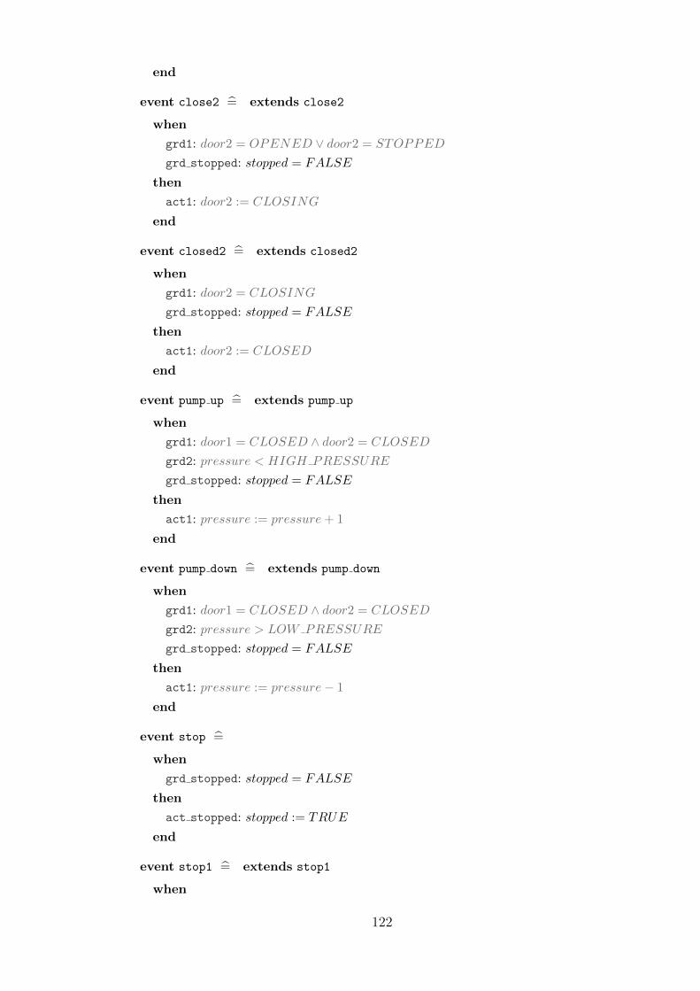
end

event close2 = extends close2

when

grd1: door2 = OPENED ∨ door2 = STOPPED

grd stopped: stopped = FALSE

then

act1: door2 := CLOSING

end

event closed2 = extends closed2

when

grd1: door2 = CLOSING

grd stopped: stopped = FALSE

then

act1: door2 := CLOSED

end

event pump up = extends pump up

when

grd1: door1 = CLOSED ∧ door2 = CLOSED

grd2: pressure < HIGH PRESSURE

grd stopped: stopped = FALSE

then

act1: pressure := pressure+ 1

end

event pump down = extends pump down

when

grd1: door1 = CLOSED ∧ door2 = CLOSED

grd2: pressure > LOW PRESSURE

grd stopped: stopped = FALSE

then

act1: pressure := pressure− 1

end

event stop =

when

grd stopped: stopped = FALSE

then

act stopped: stopped := TRUE

end

event stop1 = extends stop1

when

122

grd1: door1 = OPENING ∨ door1 = CLOSING

grd stopped: stopped = FALSE

then

act1: door1 := STOPPED

end

event stop2 = extends stop2

when

grd1: door2 = OPENING ∨ door2 = CLOSING

grd stopped: stopped = FALSE

then

act1: door2 := STOPPED

end

event stopped =

when

grd: stopped = TRUE

then

skip

end

end

A.4 Context C2

context c2 extends c0

constants

OK DEGRADED BROKEN DOOR CONDITION

axioms

axm1: DOOR CONDITION = 0, 1, 2axm2: BROKEN = 0

axm3: DEGRADED = 1

axm4: OK = 2

axm5: DOOR CONDITION ⊂ N

end

123

A.5 Machine M2

machine m2 refines m1 sees c2

variables

door1 door2 pressure stopped door1 cond door2 cond obj presence

invariants

inv1: door1 cond ∈ DOOR CONDITION

inv2: door2 cond ∈ DOOR CONDITION

inv3: obj presence ∈ BOOL

inv4: door1 cond = BROKEN ∨ door2 cond = BROKEN ∨(door1 cond = DEGRADED ∧ door2 cond = DEGRADED ∧obj presence = FALSE)⇔ stopped = TRUE

events

event INITIALISATION

extended

then

act1: door1 := CLOSED

act2: door2 := CLOSED

act3: pressure := HIGH PRESSURE

act4: stopped := FALSE

act2 0: door1 cond := OK

act2 1: door2 cond := OK

act2 2: obj presence := FALSE

end

event open1 = extends open1

when

grd1: door1 = CLOSED ∨ door1 = STOPPED

grd2: pressure = LOW PRESSURE

grd3: door2 = CLOSED

grd stopped: stopped = FALSE

then

act1: door1 := OPENING

end

event opened1 = extends opened1

when

grd1: door1 = OPENING

grd stopped: stopped = FALSE

then

act1: door1 := OPENED

end

124

event close1 = extends close1

when

grd1: door1 = OPENED ∨ door1 = STOPPED

grd stopped: stopped = FALSE

then

act1: door1 := CLOSING

end

event closed1 = extends closed1

when

grd1: door1 = CLOSING

grd stopped: stopped = FALSE

then

act1: door1 := CLOSED

end

event open2 = extends open2

when

grd1: door2 = CLOSED ∨ door2 = STOPPED

grd2: pressure = HIGH PRESSURE

grd3: door1 = CLOSED

grd stopped: stopped = FALSE

then

act1: door2 := OPENING

end

event opened2 = extends opened2

when

grd1: door2 = OPENING

grd stopped: stopped = FALSE

then

act1: door2 := OPENED

end

event close2 = extends close2

when

grd1: door2 = OPENED ∨ door2 = STOPPED

grd stopped: stopped = FALSE

then

act1: door2 := CLOSING

end

event closed2 = extends closed2

when

grd1: door2 = CLOSING

125

grd stopped: stopped = FALSE

then

act1: door2 := CLOSED

end

event pump up = extends pump up

when

grd1: door1 = CLOSED ∧ door2 = CLOSED

grd2: pressure < HIGH PRESSURE

grd stopped: stopped = FALSE

then

act1: pressure := pressure+ 1

end

event pump down = extends pump down

when

grd1: door1 = CLOSED ∧ door2 = CLOSED

grd2: pressure > LOW PRESSURE

grd stopped: stopped = FALSE

then

act1: pressure := pressure− 1

end

event break = extends stop

any

d1c d2c

where

grd stopped: stopped = FALSE

grd2 0: d1c ∈ DOOR CONDITION ∧ d1c ≤ door1 cond

grd2 1: d2c ∈ DOOR CONDITION ∧ d2c ≤ door2 cond

grd2 2: d1c = BROKEN ∨ d2c = BROKEN

grd2 3: door1 cond 6= BROKEN ∧ door2 cond 6= BROKEN

grd2 4: door1 cond = DEGRADED ∧ door2 cond = DEGRADED⇒obj presence = TRUE

then

act stopped: stopped := TRUE

act2 0: door1 cond, door2 cond := d1c, d2c

end

event stop1 = extends stop1

when

grd1: door1 = OPENING ∨ door1 = CLOSING

grd stopped: stopped = FALSE

then

126

act1: door1 := STOPPED

end

event stop2 = extends stop2

when

grd1: door2 = OPENING ∨ door2 = CLOSING

grd stopped: stopped = FALSE

then

act1: door2 := STOPPED

end

event detect =

when

grd0: door1 cond ∈ OK,DEGRADEDgrd1: door2 cond ∈ OK,DEGRADEDgrd2: door1 cond = OK ∨ door2 cond = OK

grd5: stopped = FALSE

then

act1: obj presence :∈ BOOL

end

event degrade =

any

d1c d2c

where

grd0: stopped = FALSE

grd1: d1c ∈ DOOR CONDITION∧d1c ∈ OK,DEGRADED∧d1c ≤ door1 cond

grd2: d2c ∈ DOOR CONDITION∧d2c ∈ OK,DEGRADED∧d2c ≤ door2 cond

grd3: (door1 cond = OK ∧ d1c = DEGRADED ∧ door2 cond = d2c) ∨(door2 cond = OK ∧ d2c = DEGRADED ∧ door1 cond = d1c)

grd4: d1c 6= DEGRADED ∨ d2c 6= DEGRADED ∨ obj presence = TRUE

then

act1: door1 cond := d1c

act2: door2 cond := d2c

end

event stopped = extends stopped

when

grd: stopped = TRUE

then

skip

end

event object leave = extends stop

when

127

grd stopped: stopped = FALSE

grd1: door1 cond = DEGRADED ∧ door2 cond = DEGRADED ∧obj presence = TRUE

then

act stopped: stopped := TRUE

act1: obj presence := FALSE

end

event stop on degrade = extends stop

when

grd stopped: stopped = FALSE

grd1: door1 cond = DEGRADED ∨ door2 cond = DEGRADED

grd2: obj presence = FALSE

grd4: door1 cond = OK ∨ door2 cond = OK

then

act stopped: stopped := TRUE

act1: door1 cond := DEGRADED

act2: door2 cond := DEGRADED

end

end

A.6 Machine M3

machine m3 refines m2 sees c2

variables

door1 door2 pressure stopped door1 cond door2 cond obj presence

events

event open1 = extends open1

when

grd1: door1 = CLOSED ∨ door1 = STOPPED

grd2: pressure = LOW PRESSURE

grd3: door2 = CLOSED

grd stopped: stopped = FALSE

grd2 1: door1 cond = OK

then

act1: door1 := OPENING

end

event opened1 = extends opened1

when

128

grd1: door1 = OPENING

grd stopped: stopped = FALSE

grd2 0: door1 cond ∈ OK,DEGRADEDgrd2 1: door2 cond ∈ OK,DEGRADEDgrd2 2: door1 cond = DEGRADED ∧ door2 cond = DEGRADED⇒

obj presence = TRUE

then

act1: door1 := OPENED

end

event close1 = extends close1

when

grd1: door1 = OPENED ∨ door1 = STOPPED

grd stopped: stopped = FALSE

grd2 0: door1 cond ∈ OK,DEGRADEDgrd2 1: door2 cond ∈ OK,DEGRADEDgrd2 2: door1 cond = DEGRADED ∧ door2 cond = DEGRADED⇒

obj presence = TRUE

then

act1: door1 := CLOSING

end

event closed1 = extends closed1

when

grd1: door1 = CLOSING

grd stopped: stopped = FALSE

grd2 0: door1 cond ∈ OK,DEGRADEDgrd2 1: door2 cond ∈ OK,DEGRADEDgrd2 2: door1 cond = DEGRADED ∧ door2 cond = DEGRADED⇒

obj presence = TRUE

then

act1: door1 := CLOSED

end

event open2 = extends open2

when

grd1: door2 = CLOSED ∨ door2 = STOPPED

grd2: pressure = HIGH PRESSURE

grd3: door1 = CLOSED

grd stopped: stopped = FALSE

grd2 0: door2 cond = OK ∨ (door1 cond = DEGRADED ∧door2 cond = DEGRADED ∧ obj presence = TRUE)

then

act1: door2 := OPENING

129

end

event opened2 = extends opened2

when

grd1: door2 = OPENING

grd stopped: stopped = FALSE

grd2 0: door1 cond ∈ OK,DEGRADEDgrd2 1: door2 cond ∈ OK,DEGRADEDgrd2 2: door1 cond = DEGRADED ∧ door2 cond = DEGRADED⇒

obj presence = TRUE

then

act1: door2 := OPENED

end

event close2 = extends close2

when

grd1: door2 = OPENED ∨ door2 = STOPPED

grd stopped: stopped = FALSE

grd2 0: door1 cond ∈ OK,DEGRADEDgrd2 1: door2 cond ∈ OK,DEGRADEDgrd2 2: door1 cond = DEGRADED ∧ door2 cond = DEGRADED⇒

obj presence = TRUE

then

act1: door2 := CLOSING

end

event closed2 = extends closed2

when

grd1: door2 = CLOSING

grd stopped: stopped = FALSE

grd2 0: door1 cond ∈ OK,DEGRADEDgrd2 1: door2 cond ∈ OK,DEGRADEDgrd2 2: door1 cond = DEGRADED ∧ door2 cond = DEGRADED⇒

obj presence = TRUE

then

act1: door2 := CLOSED

end

event pump up = extends pump up

when

grd1: door1 = CLOSED ∧ door2 = CLOSED

grd2: pressure < HIGH PRESSURE

grd stopped: stopped = FALSE

grd2 0: door1 cond ∈ OK,DEGRADED

130

grd2 1: door2 cond = OK ∨ (door1 cond = DEGRADED ∧door2 cond = DEGRADED ∧ obj presence = TRUE)

then

act1: pressure := pressure+ 1

end

event pump down = extends pump down

when

grd1: door1 = CLOSED ∧ door2 = CLOSED

grd2: pressure > LOW PRESSURE

grd stopped: stopped = FALSE

grd2 0: door1 cond = OK

then

act1: pressure := pressure− 1

end

event INITIALISATION

extended

then

act1: door1 := CLOSED

act2: door2 := CLOSED

act3: pressure := HIGH PRESSURE

act4: stopped := FALSE

act2 0: door1 cond := OK

act2 1: door2 cond := OK

act2 2: obj presence := FALSE

end

event break = extends break

any

d1c d2c

where

grd stopped: stopped = FALSE

grd2 0: d1c ∈ DOOR CONDITION ∧ d1c ≤ door1 cond

grd2 1: d2c ∈ DOOR CONDITION ∧ d2c ≤ door2 cond

grd2 2: d1c = BROKEN ∨ d2c = BROKEN

grd2 3: door1 cond 6= BROKEN ∧ door2 cond 6= BROKEN

grd2 4: door1 cond = DEGRADED ∧ door2 cond = DEGRADED⇒obj presence = TRUE

then

act stopped: stopped := TRUE

act2 0: door1 cond, door2 cond := d1c, d2c

end

event stop1 = extends stop1

131

when

grd1: door1 = OPENING ∨ door1 = CLOSING

grd stopped: stopped = FALSE

then

act1: door1 := STOPPED

end

event stop2 = extends stop2

when

grd1: door2 = OPENING ∨ door2 = CLOSING

grd stopped: stopped = FALSE

then

act1: door2 := STOPPED

end

event degrade = extends degrade

any

d1c d2c

where

grd0: stopped = FALSE

grd1: d1c ∈ DOOR CONDITION∧d1c ∈ OK,DEGRADED∧d1c ≤ door1 cond

grd2: d2c ∈ DOOR CONDITION∧d2c ∈ OK,DEGRADED∧d2c ≤ door2 cond

grd3: (door1 cond = OK ∧ d1c = DEGRADED ∧ door2 cond = d2c) ∨(door2 cond = OK ∧ d2c = DEGRADED ∧ door1 cond = d1c)

grd4: d1c 6= DEGRADED ∨ d2c 6= DEGRADED ∨ obj presence = TRUE

then

act1: door1 cond := d1c

act2: door2 cond := d2c

end

event detect = extends detect

when

grd0: door1 cond ∈ OK,DEGRADEDgrd1: door2 cond ∈ OK,DEGRADEDgrd2: door1 cond = OK ∨ door2 cond = OK

grd5: stopped = FALSE

then

act1: obj presence :∈ BOOL

end

event stopped = extends stopped

when

grd: stopped = TRUE

then

132

skip

end

event object leave = extends object leave

when

grd stopped: stopped = FALSE

grd1: door1 cond = DEGRADED ∧ door2 cond = DEGRADED ∧obj presence = TRUE

then

act stopped: stopped := TRUE

act1: obj presence := FALSE

end

event stop on degrade = extends stop on degrade

when

grd stopped: stopped = FALSE

grd1: door1 cond = DEGRADED ∨ door2 cond = DEGRADED

grd2: obj presence = FALSE

grd4: door1 cond = OK ∨ door2 cond = OK

then

act stopped: stopped := TRUE

act1: door1 cond := DEGRADED

act2: door2 cond := DEGRADED

end

end

A.7 Machine M4

machine m4 refines m3 sees c2

variables

door1 door2 pressure stopped door2 cond obj presence

door1 pos cond door1 closed cond door1 opened cond door1 motor cond

invariants

inv door1 pos cond: door1 pos cond ∈ BOOL

inv door1 closed cond: door1 closed cond ∈ BOOL

inv door1 opened cond: door1 opened cond ∈ BOOL

inv door1 motor cond: door1 motor cond ∈ BOOL

inv door1 sensors conditions OK: door1 cond = OK⇔door1 pos cond = TRUE ∧ door1 closed cond = TRUE ∧door1 opened cond = TRUE ∧ door1 motor cond = TRUE

133

inv door1 sensors conditions DEGRADED: door1 cond = DEGRADED⇔door1 motor cond = TRUE ∧((door1 pos cond = FALSE ∧ door1 opened cond = TRUE ∧

door1 closed cond = TRUE) ∨(door1 pos cond = TRUE ∧

(door1 opened cond = FALSE ∨ door1 closed cond = FALSE)))

inv door1 sensors conditions BROKEN: door1 cond = BROKEN ⇔door1 motor cond = FALSE ∨ (door1 pos cond = FALSE ∧(door1 opened cond = FALSE ∨ door1 closed cond = FALSE))

events

event INITIALISATION

then

act1: door1 := CLOSED

act2: door2 := CLOSED

act3: pressure := HIGH PRESSURE

act4: stopped := FALSE

act2 1: door2 cond := OK

act2 2: obj presence := FALSE

act4 2: door1 pos cond := TRUE

act4 3: door1 closed cond := TRUE

act4 4: door1 opened cond := TRUE

act4 5: door1 motor cond := TRUE

end

event open1 = refines open1

when

grd1: door1 = CLOSED ∨ door1 = STOPPED

grd2: pressure = LOW PRESSURE

grd3: door2 = CLOSED

grd stopped: stopped = FALSE

grd cond: door1 pos cond = TRUE ∧ door1 closed cond = TRUE ∧door1 opened cond = TRUE ∧ door1 motor cond = TRUE

then

act1: door1 := OPENING

end

event opened1 = refines opened1

when

grd1: door1 = OPENING

grd stopped: stopped = FALSE

grd4 0: door1 motor cond = TRUE

grd4 1: (door1 pos cond = TRUE ∧ door1 closed cond = TRUE ∧door1 opened cond = TRUE) ∨

134

(door1 pos cond = FALSE ∧ door1 opened cond = TRUE ∧door1 closed cond = TRUE) ∨

(door1 pos cond = TRUE ∧(door1 opened cond = FALSE ∨ door1 closed cond = FALSE))

grd4 2: door2 cond ∈ OK,DEGRADEDgrd4 3: door1 motor cond = TRUE ∧

((door1 pos cond = FALSE ∧ door1 opened cond = TRUE ∧door1 closed cond = TRUE) ∨

(door1 pos cond = TRUE ∧(door1 opened cond = FALSE ∨ door1 closed cond = FALSE))) ∧

door2 cond = DEGRADED⇒ obj presence = TRUE

then

act1: door1 := OPENED

end

event close1 = refines close1

when

grd1: door1 = OPENED ∨ door1 = STOPPED

grd stopped: stopped = FALSE

grd4 0: door1 motor cond = TRUE

grd4 1: (door1 pos cond = TRUE ∧ door1 closed cond = TRUE ∧door1 opened cond = TRUE) ∨

(door1 pos cond = FALSE ∧ door1 opened cond = TRUE ∧door1 closed cond = TRUE) ∨

(door1 pos cond = TRUE ∧(door1 opened cond = FALSE ∨ door1 closed cond = FALSE))

grd4 2: door2 cond ∈ OK,DEGRADEDgrd4 3: door1 motor cond = TRUE ∧

((door1 pos cond = FALSE ∧ door1 opened cond = TRUE ∧door1 closed cond = TRUE) ∨

(door1 pos cond = TRUE ∧(door1 opened cond = FALSE ∨ door1 closed cond = FALSE))) ∧

door2 cond = DEGRADED⇒ obj presence = TRUE

then

act1: door1 := CLOSING

end

event closed1 = refines closed1

when

grd1: door1 = CLOSING

grd stopped: stopped = FALSE

grd4 0: door1 motor cond = TRUE

grd4 1: (door1 pos cond = TRUE ∧ door1 closed cond = TRUE ∧door1 opened cond = TRUE) ∨

135

(door1 pos cond = FALSE ∧ door1 opened cond = TRUE ∧door1 closed cond = TRUE) ∨

(door1 pos cond = TRUE ∧(door1 opened cond = FALSE ∨ door1 closed cond = FALSE))

grd4 2: door2 cond ∈ OK,DEGRADEDgrd4 3: door1 motor cond = TRUE ∧

((door1 pos cond = FALSE ∧ door1 opened cond = TRUE ∧door1 closed cond = TRUE) ∨

(door1 pos cond = TRUE ∧(door1 opened cond = FALSE ∨ door1 closed cond = FALSE))) ∧

door2 cond = DEGRADED⇒ obj presence = TRUE

then

act1: door1 := CLOSED

end

event open2 = refines open2

when

grd1: door2 = CLOSED ∨ door2 = STOPPED

grd2: pressure = HIGH PRESSURE

grd3: door1 = CLOSED

grd stopped: stopped = FALSE

grd2 0: door2 cond = OK ∨ ((door1 motor cond = TRUE ∧((door1 pos cond = FALSE ∧ door1 opened cond = TRUE ∧

door1 closed cond = TRUE) ∨(door1 pos cond = TRUE ∧

(door1 opened cond = FALSE ∨ door1 closed cond = FALSE)))) ∧door2 cond = DEGRADED ∧ obj presence = TRUE)

then

act1: door2 := OPENING

end

event opened2 = refines opened2

when

grd1: door2 = OPENING

grd stopped: stopped = FALSE

grd4 0: door1 motor cond = TRUE

grd4 1: (door1 pos cond = TRUE ∧ door1 closed cond = TRUE ∧door1 opened cond = TRUE) ∨

(door1 pos cond = FALSE ∧ door1 opened cond = TRUE ∧door1 closed cond = TRUE) ∨

(door1 pos cond = TRUE ∧(door1 opened cond = FALSE ∨ door1 closed cond = FALSE))

grd4 2: door2 cond ∈ OK,DEGRADED

136

grd4 3: door1 motor cond = TRUE ∧((door1 pos cond = FALSE ∧ door1 opened cond = TRUE ∧

door1 closed cond = TRUE) ∨(door1 pos cond = TRUE ∧

(door1 opened cond = FALSE ∨ door1 closed cond = FALSE))) ∧door2 cond = DEGRADED⇒ obj presence = TRUE

then

act1: door2 := OPENED

end

event close2 = refines close2

when

grd1: door2 = OPENED ∨ door2 = STOPPED

grd stopped: stopped = FALSE

grd4 0: door1 motor cond = TRUE

grd4 1: (door1 pos cond = TRUE ∧ door1 closed cond = TRUE ∧door1 opened cond = TRUE) ∨

(door1 pos cond = FALSE ∧ door1 opened cond = TRUE ∧door1 closed cond = TRUE) ∨

(door1 pos cond = TRUE ∧(door1 opened cond = FALSE ∨ door1 closed cond = FALSE))

grd4 2: door2 cond ∈ OK,DEGRADEDgrd4 3: door1 motor cond = TRUE ∧

((door1 pos cond = FALSE ∧ door1 opened cond = TRUE ∧door1 closed cond = TRUE) ∨

(door1 pos cond = TRUE ∧(door1 opened cond = FALSE ∨ door1 closed cond = FALSE))) ∧

door2 cond = DEGRADED⇒ obj presence = TRUE

then

act1: door2 := CLOSING

end

event closed2 = refines closed2

when

grd1: door2 = CLOSING

grd stopped: stopped = FALSE

grd4 0: door1 motor cond = TRUE

grd4 1: (door1 pos cond = TRUE ∧ door1 closed cond = TRUE ∧door1 opened cond = TRUE) ∨

(door1 pos cond = FALSE ∧ door1 opened cond = TRUE ∧door1 closed cond = TRUE) ∨

(door1 pos cond = TRUE ∧(door1 opened cond = FALSE ∨ door1 closed cond = FALSE))

grd4 2: door2 cond ∈ OK,DEGRADED

137

grd4 3: door1 motor cond = TRUE ∧((door1 pos cond = FALSE ∧ door1 opened cond = TRUE ∧

door1 closed cond = TRUE) ∨(door1 pos cond = TRUE ∧

(door1 opened cond = FALSE ∨ door1 closed cond = FALSE))) ∧door2 cond = DEGRADED⇒ obj presence = TRUE

then

act1: door2 := CLOSED

end

event pump up = refines pump up

when

grd1: door1 = CLOSED ∧ door2 = CLOSED

grd2: pressure < HIGH PRESSURE

grd stopped: stopped = FALSE

grd4 0: door1 motor cond = TRUE

grd4 1: (door1 pos cond = TRUE ∧ door1 closed cond = TRUE ∧door1 opened cond = TRUE) ∨

(door1 pos cond = FALSE ∧ door1 opened cond = TRUE ∧door1 closed cond = TRUE) ∨

(door1 pos cond = TRUE ∧(door1 opened cond = FALSE ∨ door1 closed cond = FALSE))

grd4 2: door2 cond = OK ∨ ((door1 motor cond = TRUE ∧((door1 pos cond = FALSE ∧ door1 opened cond = TRUE ∧

door1 closed cond = TRUE) ∨(door1 pos cond = TRUE ∧

(door1 opened cond = FALSE ∨ door1 closed cond = FALSE)))) ∧door2 cond = DEGRADED ∧ obj presence = TRUE)

then

act1: pressure := pressure+ 1

end

event pump down = refines pump down

when

grd1: door1 = CLOSED ∧ door2 = CLOSED

grd2: pressure > LOW PRESSURE

grd stopped: stopped = FALSE

grd4 0: door1 pos cond = TRUE ∧ door1 closed cond = TRUE ∧door1 opened cond = TRUE ∧ door1 motor cond = TRUE

then

act1: pressure := pressure− 1

end

event break1 = refines break

138

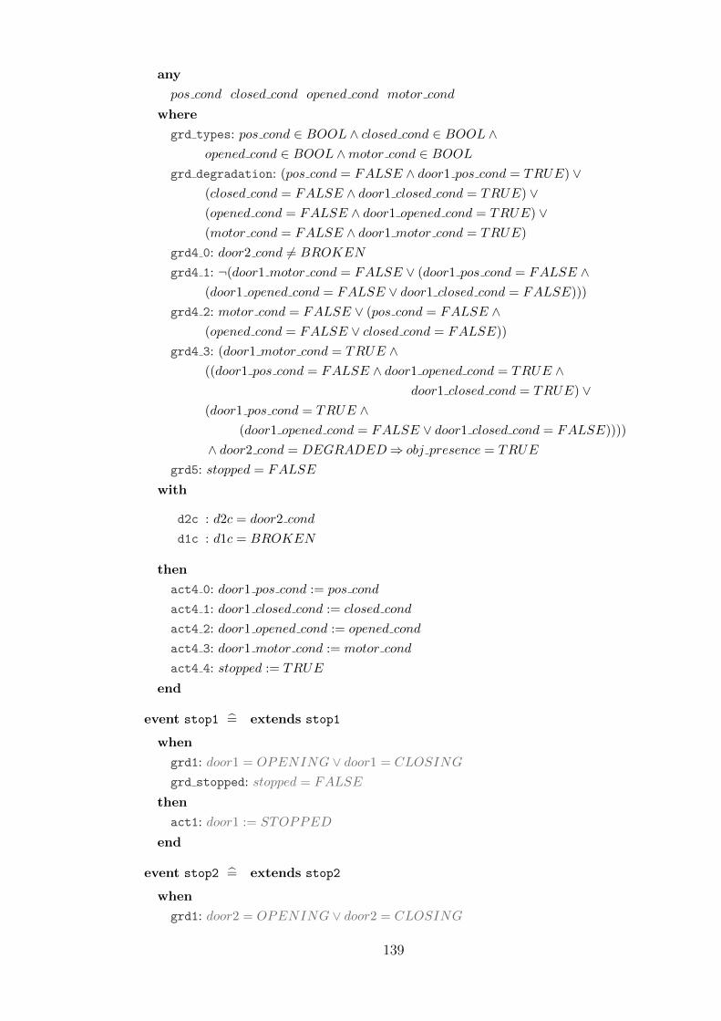
any

pos cond closed cond opened cond motor cond

where

grd types: pos cond ∈ BOOL ∧ closed cond ∈ BOOL ∧opened cond ∈ BOOL ∧motor cond ∈ BOOL

grd degradation: (pos cond = FALSE ∧ door1 pos cond = TRUE) ∨(closed cond = FALSE ∧ door1 closed cond = TRUE) ∨(opened cond = FALSE ∧ door1 opened cond = TRUE) ∨(motor cond = FALSE ∧ door1 motor cond = TRUE)

grd4 0: door2 cond 6= BROKEN

grd4 1: ¬(door1 motor cond = FALSE ∨ (door1 pos cond = FALSE ∧(door1 opened cond = FALSE ∨ door1 closed cond = FALSE)))

grd4 2: motor cond = FALSE ∨ (pos cond = FALSE ∧(opened cond = FALSE ∨ closed cond = FALSE))

grd4 3: (door1 motor cond = TRUE ∧((door1 pos cond = FALSE ∧ door1 opened cond = TRUE ∧

door1 closed cond = TRUE) ∨(door1 pos cond = TRUE ∧

(door1 opened cond = FALSE ∨ door1 closed cond = FALSE))))

∧ door2 cond = DEGRADED⇒ obj presence = TRUE

grd5: stopped = FALSE

with

d2c : d2c = door2 cond

d1c : d1c = BROKEN

then

act4 0: door1 pos cond := pos cond

act4 1: door1 closed cond := closed cond

act4 2: door1 opened cond := opened cond

act4 3: door1 motor cond := motor cond

act4 4: stopped := TRUE

end

event stop1 = extends stop1

when

grd1: door1 = OPENING ∨ door1 = CLOSING

grd stopped: stopped = FALSE

then

act1: door1 := STOPPED

end

event stop2 = extends stop2

when

grd1: door2 = OPENING ∨ door2 = CLOSING

139

grd stopped: stopped = FALSE

then

act1: door2 := STOPPED

end

event degrade door1 = refines degrade

any

pos cond closed cond opened cond motor cond

where

grd types: pos cond ∈ BOOL ∧ closed cond ∈ BOOL ∧opened cond ∈ BOOL ∧motor cond ∈ BOOL

grd degradation: (pos cond = FALSE ∧ door1 pos cond = TRUE) ∨(closed cond = FALSE ∧ door1 closed cond = TRUE) ∨(opened cond = FALSE ∧ door1 opened cond = TRUE) ∨

(motor cond = FALSE ∧ door1 motor cond = TRUE)

grd stopped: stopped = FALSE

grd1: door1 pos cond = TRUE ∧ door1 closed cond = TRUE ∧door1 opened cond = TRUE ∧ door1 motor cond = TRUE

grd7: door2 cond = DEGRADED⇒ obj presence = TRUE

grd glue: motor cond = TRUE ∧((pos cond = FALSE ∧ opened cond = TRUE ∧

closed cond = TRUE) ∨(pos cond = TRUE ∧

(opened cond = FALSE ∨ closed cond = FALSE)))

with

d2c : d2c = door2 cond

d1c : d1c = DEGRADED

then

act4 0: door1 pos cond := pos cond

act4 1: door1 closed cond := closed cond

act4 2: door1 opened cond := opened cond

act4 3: door1 motor cond := motor cond

end

event degrade door2 = refines degrade

when

grd stopped: stopped = FALSE

grd4 0: door1 motor cond = TRUE

grd4 1: (door1 pos cond = TRUE ∧ door1 closed cond = TRUE ∧door1 opened cond = TRUE) ∨

(door1 pos cond = FALSE ∧ door1 opened cond = TRUE ∧door1 closed cond = TRUE) ∨

(door1 pos cond = TRUE ∧(door1 opened cond = FALSE ∨ door1 closed cond = FALSE))

140

grd4 2: (door1 motor cond = TRUE ∧((door1 pos cond = FALSE ∧ door1 opened cond = TRUE ∧

door1 closed cond = TRUE) ∨(door1 pos cond = TRUE ∧

(door1 opened cond = FALSE ∨ door1 closed cond = FALSE))))⇒obj presence = TRUE

grd4 3: door2 cond = OK

with

d2c : d2c = DEGRADED

d1c : (d1c = OK⇔ door1 pos cond = TRUE ∧ door1 closed cond = TRUE ∧door1 opened cond = TRUE ∧ door1 motor cond = TRUE) ∧

(d1c = DEGRADED⇔ (door1 motor cond = TRUE ∧((door1 pos cond = FALSE ∧ door1 opened cond = TRUE ∧

door1 closed cond = TRUE) ∨(door1 pos cond = TRUE ∧

(door1 opened cond = FALSE ∨ door1 closed cond = FALSE)))))

then

act: door2 cond := DEGRADED

end

event stop on degrade door1 = refines stop on degrade

any

pos cond closed cond opened cond motor cond

where

grd types: pos cond ∈ BOOL ∧ closed cond ∈ BOOL ∧opened cond ∈ BOOL ∧motor cond ∈ BOOL

grd degradation: (pos cond = FALSE ∧ door1 pos cond = TRUE) ∨(closed cond = FALSE ∧ door1 closed cond = TRUE) ∨(opened cond = FALSE ∧ door1 opened cond = TRUE) ∨(motor cond = FALSE ∧ door1 motor cond = TRUE)

grd stopped: stopped = FALSE

grd1: door2 cond = DEGRADED

grd2: obj presence = FALSE

grd glue: motor cond = TRUE ∧((pos cond = FALSE ∧ opened cond = TRUE ∧

closed cond = TRUE) ∨(pos cond = TRUE ∧

(opened cond = FALSE ∨ closed cond = FALSE)))

then

act4 0: door1 pos cond := pos cond

act4 1: door1 closed cond := closed cond

act4 2: door1 opened cond := opened cond

act4 3: door1 motor cond := motor cond

141

act2: stopped := TRUE

end

event stop on degrade door2 = refines stop on degrade

when

grd stopped: stopped = FALSE

grd1: door2 cond = OK

grd2: obj presence = FALSE

grd3: door1 motor cond = TRUE ∧((door1 pos cond = FALSE ∧ door1 opened cond = TRUE ∧

door1 closed cond = TRUE) ∨(door1 pos cond = TRUE ∧

(door1 opened cond = FALSE ∨ door1 closed cond = FALSE)))

then

act1: door2 cond := DEGRADED

act2: stopped := TRUE

end

event detect = refines detect

when

grd4 0: door1 motor cond = TRUE

grd4 1: (door1 pos cond = TRUE ∧ door1 closed cond = TRUE ∧door1 opened cond = TRUE) ∨

(door1 pos cond = FALSE ∧ door1 opened cond = TRUE ∧door1 closed cond = TRUE) ∨

(door1 pos cond = TRUE ∧(door1 opened cond = FALSE ∨ door1 closed cond = FALSE))

grd1: door2 cond ∈ OK,DEGRADEDgrd2: (door1 pos cond = TRUE ∧ door1 closed cond = TRUE ∧

door1 opened cond = TRUE ∧ door1 motor cond = TRUE) ∨door2 cond = OK

grd5: stopped = FALSE

then

act1: obj presence :∈ BOOL

end

event stopped = extends stopped

when

grd: stopped = TRUE

then

skip

end

event object leave = refines object leave

when

142

grd stopped: stopped = FALSE

grd1: door1 motor cond = TRUE ∧((door1 pos cond = FALSE ∧ door1 opened cond = TRUE ∧

door1 closed cond = TRUE) ∨(door1 pos cond = TRUE ∧

(door1 opened cond = FALSE ∨ door1 closed cond = FALSE)))

grd2: door2 cond = DEGRADED

grd3: obj presence = TRUE

then

act1: obj presence := FALSE

act stopped: stopped := TRUE

end

event break2 = refines break

when

grd4 0: door2 cond 6= BROKEN

grd4 1: ¬(door1 motor cond = FALSE ∨ (door1 pos cond = FALSE ∧(door1 opened cond = FALSE ∨ door1 closed cond = FALSE)))

grd4 3: (door1 motor cond = TRUE ∧((door1 pos cond = FALSE ∧ door1 opened cond = TRUE ∧

door1 closed cond = TRUE) ∨(door1 pos cond = TRUE ∧

(door1 opened cond = FALSE ∨ door1 closed cond = FALSE)))) ∧door2 cond = DEGRADED⇒ obj presence = TRUE

grd5: stopped = FALSE

with

d2c : d2c = BROKEN

d1c : (d1c = OK⇔ door1 pos cond = TRUE ∧ door1 closed cond = TRUE ∧door1 opened cond = TRUE ∧ door1 motor cond = TRUE) ∧

(d1c = DEGRADED⇔ (door1 motor cond = TRUE ∧((door1 pos cond = FALSE ∧ door1 opened cond = TRUE ∧

door1 closed cond = TRUE) ∨(door1 pos cond = TRUE ∧

(door1 opened cond = FALSE ∨ door1 closed cond = FALSE)))))

then

act4 1: door2 cond := BROKEN

act4 4: stopped := TRUE

end

end

143

A.8 Context C5

context c5 extends c2

sets

PHASE

constants

ENV DET CONT PRED min door max door

axioms

axm1: partition(PHASE, ENV , DET, CONT, PRED)axm2: min door < max door

axm3: min door ∈ N ∧max door ∈ Naxm4: max door −min door > 1

end

A.9 Machine M5

machine m5 refines m4 sees c5

variables

door1 door2 pressure stopped obj presence door2 cond

door1 pos cond door1 closed cond door1 opened cond door1 motor cond

phase door1 motor door1 motor cond detected

door1 pos door1 pos predicted door1 pos cond detected

door1 opened door1 opened predicted door1 opened cond detected

door1 closed door1 closed predicted door1 closed cond detected

invariants

inv phase: phase ∈ PHASE

inv1: door1 pos ∈ Zinv2: door1 opened ∈ BOOL

inv3: door1 closed ∈ BOOL

inv4: door1 pos predicted ∈ Zinv5: door1 opened predicted ∈ BOOL

inv6: door1 closed predicted ∈ BOOL

inv7: door1 motor ∈ −1, 0, 1inv10: door1 pos cond detected ∈ BOOL

inv11: door1 opened cond detected ∈ BOOL

inv12: door1 closed cond detected ∈ BOOL

inv13: door1 motor cond detected ∈ BOOL

events

144

event INITIALISATION

extended

then

act1: door1 := CLOSED

act2: door2 := CLOSED

act3: pressure := HIGH PRESSURE

act4: stopped := FALSE

act2 1: door2 cond := OK

act2 2: obj presence := FALSE

act4 2: door1 pos cond := TRUE

act4 3: door1 closed cond := TRUE

act4 4: door1 opened cond := TRUE

act4 5: door1 motor cond := TRUE

act phase: phase := ENV

act5 1: door1 pos := 0

act5 2: door1 pos predicted := 0

act5 3: door1 opened := FALSE

act5 4: door1 opened predicted := FALSE

act5 5: door1 closed := TRUE

act5 6: door1 closed predicted := FALSE

act5 7: door1 motor := 0

end

event cycle sense =

when

grd phase: phase = ENV

grd stopped: stopped = FALSE

then

act phase: phase := DET

act5 1: door1 pos :∈ Zact5 2: door1 opened :∈ BOOL

act5 3: door1 closed :∈ BOOL

end

event cycle detect =

when

grd phase: phase = DET

grd stopped: stopped = FALSE

then

act phase: phase := CONT

act5 1: door1 pos cond detected := bool(door1 pos cond = TRUE ∧(min door ≤ door1 pos ∧ door1 pos ≤ max door) ∧(door1 opened cond = TRUE ∧ door1 opened = TRUE⇒

door1 pos = max door) ∧

145

(door1 closed cond = TRUE ∧ door1 closed = TRUE⇒door1 pos = min door) ∧

(door1 pos = door1 pos predicted))

act5 2: door1 closed cond detected :=

bool(door1 closed cond = TRUE ∧ (door1 closed = door1 closed predicted))

act5 3: door1 opened cond detected :=

bool(door1 opened cond = TRUE∧(door1 opened = door1 opened predicted))

act5 4: door1 motor cond detected := bool(door1 motor cond = TRUE ∧((door1 pos = door1 pos predicted)∨(door1 closed = door1 closed predicted)∨

(door1 opened = door1 opened predicted)))

end

event cycle predict =

when

grd phase: phase = PRED

grd stopped: stopped = FALSE

then

act phase: phase := ENV

act5 1: door1 pos predicted := door1 pos+ door1 motor

act5 2: door1 opened predicted := bool(

(door1 motor = 1 ∧ door1 pos = max door − 1) ∨(door1 motor = 0 ∧ door1 opened = TRUE))

act5 3: door1 closed predicted := bool(

(door1 motor = −1 ∧ door1 pos = min door + 1) ∨(door1 motor = 0 ∧ door1 closed = TRUE))

end

event open1 = extends open1

when

grd1: door1 = CLOSED ∨ door1 = STOPPED

grd2: pressure = LOW PRESSURE

grd3: door2 = CLOSED

grd stopped: stopped = FALSE

grd cond: door1 pos cond = TRUE ∧ door1 closed cond = TRUE ∧door1 opened cond = TRUE ∧ door1 motor cond = TRUE

grd phase: phase = CONT

grd pos: door1 pos cond = TRUE⇒ door1 pos < max door ∧(door1 pos = min door⇒ door1 = CLOSED) ∧(door1 pos > min door⇒ door1 = STOPPED)

grd closed: door1 closed cond = TRUE⇒(door1 closed = TRUE⇒ door1 = CLOSED)

grd opened: door1 opened cond = TRUE⇒ door1 opened = FALSE

then

146

act1: door1 := OPENING

act phase: phase := PRED

act motor: door1 motor := 1

end

event opened1 = extends opened1

when

grd1: door1 = OPENING

grd stopped: stopped = FALSE

grd4 0: door1 motor cond = TRUE

grd4 1: (door1 pos cond = TRUE ∧ door1 closed cond = TRUE ∧door1 opened cond = TRUE) ∨

(door1 pos cond = FALSE ∧ door1 opened cond = TRUE ∧door1 closed cond = TRUE) ∨

(door1 pos cond = TRUE ∧(door1 opened cond = FALSE ∨ door1 closed cond = FALSE))

grd4 2: door2 cond ∈ OK,DEGRADEDgrd4 3: door1 motor cond = TRUE ∧

((door1 pos cond = FALSE ∧ door1 opened cond = TRUE ∧door1 closed cond = TRUE) ∨

(door1 pos cond = TRUE ∧(door1 opened cond = FALSE ∨ door1 closed cond = FALSE))) ∧

door2 cond = DEGRADED⇒ obj presence = TRUE

grd phase: phase = CONT

grd pos: door1 pos cond = TRUE⇒ door1 pos = max door

grd closed: door1 closed cond = TRUE⇒ door1 closed = FALSE

grd opened: door1 opened cond = TRUE⇒ door1 opened = TRUE

then

act1: door1 := OPENED

act phase: phase := PRED

act motor: door1 motor := 0

end

event close1 = extends close1

when

grd1: door1 = OPENED ∨ door1 = STOPPED

grd stopped: stopped = FALSE

grd4 0: door1 motor cond = TRUE

grd4 1: (door1 pos cond = TRUE ∧ door1 closed cond = TRUE ∧door1 opened cond = TRUE) ∨

(door1 pos cond = FALSE ∧ door1 opened cond = TRUE ∧door1 closed cond = TRUE) ∨

(door1 pos cond = TRUE ∧(door1 opened cond = FALSE ∨ door1 closed cond = FALSE))

147

grd4 2: door2 cond ∈ OK,DEGRADEDgrd4 3: door1 motor cond = TRUE ∧

((door1 pos cond = FALSE ∧ door1 opened cond = TRUE ∧door1 closed cond = TRUE) ∨

(door1 pos cond = TRUE ∧(door1 opened cond = FALSE ∨ door1 closed cond = FALSE))) ∧

door2 cond = DEGRADED⇒ obj presence = TRUE

grd phase: phase = CONT

grd pos: door1 pos cond = TRUE⇒ door1 pos > min door ∧(door1 pos = max door⇒ door1 = OPENED) ∧(door1 pos < max door⇒ door1 = STOPPED)

grd closed: door1 closed cond = TRUE⇒ door1 closed = FALSE

grd opened: door1 opened cond = TRUE⇒(door1 opened = TRUE⇒ door1 = OPENED)

then

act1: door1 := CLOSING

act phase: phase := PRED

act motor: door1 motor := −1end

event closed1 = extends closed1

when

grd1: door1 = CLOSING

grd stopped: stopped = FALSE

grd4 0: door1 motor cond = TRUE

grd4 1: (door1 pos cond = TRUE ∧ door1 closed cond = TRUE ∧door1 opened cond = TRUE) ∨

(door1 pos cond = FALSE ∧ door1 opened cond = TRUE ∧door1 closed cond = TRUE) ∨

(door1 pos cond = TRUE ∧(door1 opened cond = FALSE ∨ door1 closed cond = FALSE))

grd4 2: door2 cond ∈ OK,DEGRADEDgrd4 3: door1 motor cond = TRUE ∧

((door1 pos cond = FALSE ∧ door1 opened cond = TRUE ∧door1 closed cond = TRUE) ∨

(door1 pos cond = TRUE ∧(door1 opened cond = FALSE ∨ door1 closed cond = FALSE))) ∧

door2 cond = DEGRADED⇒ obj presence = TRUE

grd phase: phase = CONT

grd pos: door1 pos cond = TRUE⇒ door1 pos = min door

grd closed: door1 closed cond = TRUE⇒ door1 closed = TRUE

grd opened: door1 opened cond = TRUE⇒ door1 opened = FALSE

then

act1: door1 := CLOSED

148

act phase: phase := PRED

act motor: door1 motor := 0

end

event open2 = extends open2

when

grd1: door2 = CLOSED ∨ door2 = STOPPED

grd2: pressure = HIGH PRESSURE

grd3: door1 = CLOSED

grd stopped: stopped = FALSE

grd2 0: door2 cond = OK ∨ ((door1 motor cond = TRUE ∧((door1 pos cond = FALSE ∧ door1 opened cond = TRUE ∧

door1 closed cond = TRUE) ∨(door1 pos cond = TRUE ∧

(door1 opened cond = FALSE ∨ door1 closed cond = FALSE)))) ∧door2 cond = DEGRADED ∧ obj presence = TRUE)

grd phase: phase = CONT

then

act1: door2 := OPENING

act phase: phase := PRED

end

event opened2 = extends opened2

when

grd1: door2 = OPENING

grd stopped: stopped = FALSE

grd4 0: door1 motor cond = TRUE

grd4 1: (door1 pos cond = TRUE ∧ door1 closed cond = TRUE ∧door1 opened cond = TRUE) ∨

(door1 pos cond = FALSE ∧ door1 opened cond = TRUE ∧door1 closed cond = TRUE) ∨

(door1 pos cond = TRUE ∧(door1 opened cond = FALSE ∨ door1 closed cond = FALSE))

grd4 2: door2 cond ∈ OK,DEGRADEDgrd4 3: door1 motor cond = TRUE ∧

((door1 pos cond = FALSE ∧ door1 opened cond = TRUE ∧door1 closed cond = TRUE) ∨

(door1 pos cond = TRUE ∧(door1 opened cond = FALSE ∨ door1 closed cond = FALSE))) ∧

door2 cond = DEGRADED⇒ obj presence = TRUE

grd phase: phase = CONT

then

act1: door2 := OPENED

act phase: phase := PRED

149

end

event close2 = extends close2

when

grd1: door2 = OPENED ∨ door2 = STOPPED

grd stopped: stopped = FALSE

grd4 0: door1 motor cond = TRUE

grd4 1: (door1 pos cond = TRUE ∧ door1 closed cond = TRUE ∧door1 opened cond = TRUE) ∨

(door1 pos cond = FALSE ∧ door1 opened cond = TRUE ∧door1 closed cond = TRUE) ∨

(door1 pos cond = TRUE ∧(door1 opened cond = FALSE ∨ door1 closed cond = FALSE))

grd4 2: door2 cond ∈ OK,DEGRADEDgrd4 3: door1 motor cond = TRUE ∧

((door1 pos cond = FALSE ∧ door1 opened cond = TRUE ∧door1 closed cond = TRUE) ∨

(door1 pos cond = TRUE ∧(door1 opened cond = FALSE ∨ door1 closed cond = FALSE))) ∧

door2 cond = DEGRADED⇒ obj presence = TRUE

grd phase: phase = CONT

then

act1: door2 := CLOSING

act phase: phase := PRED

end

event closed2 = extends closed2

when

grd1: door2 = CLOSING

grd stopped: stopped = FALSE

grd4 0: door1 motor cond = TRUE

grd4 1: (door1 pos cond = TRUE ∧ door1 closed cond = TRUE ∧door1 opened cond = TRUE) ∨

(door1 pos cond = FALSE ∧ door1 opened cond = TRUE ∧door1 closed cond = TRUE) ∨

(door1 pos cond = TRUE ∧(door1 opened cond = FALSE ∨ door1 closed cond = FALSE))

grd4 2: door2 cond ∈ OK,DEGRADEDgrd4 3: door1 motor cond = TRUE ∧

((door1 pos cond = FALSE ∧ door1 opened cond = TRUE ∧door1 closed cond = TRUE) ∨

(door1 pos cond = TRUE ∧(door1 opened cond = FALSE ∨ door1 closed cond = FALSE))) ∧

door2 cond = DEGRADED⇒ obj presence = TRUE

150

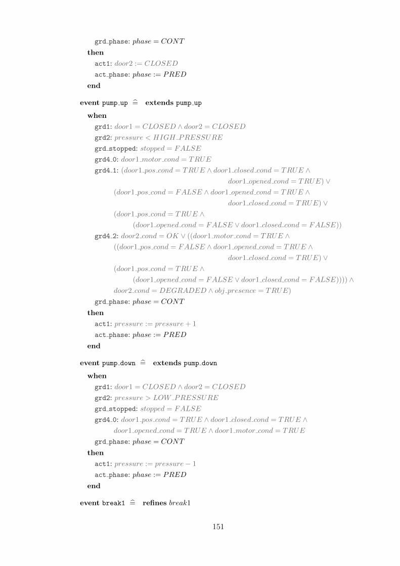
grd phase: phase = CONT

then

act1: door2 := CLOSED

act phase: phase := PRED

end

event pump up = extends pump up

when

grd1: door1 = CLOSED ∧ door2 = CLOSED

grd2: pressure < HIGH PRESSURE

grd stopped: stopped = FALSE

grd4 0: door1 motor cond = TRUE

grd4 1: (door1 pos cond = TRUE ∧ door1 closed cond = TRUE ∧door1 opened cond = TRUE) ∨

(door1 pos cond = FALSE ∧ door1 opened cond = TRUE ∧door1 closed cond = TRUE) ∨

(door1 pos cond = TRUE ∧(door1 opened cond = FALSE ∨ door1 closed cond = FALSE))

grd4 2: door2 cond = OK ∨ ((door1 motor cond = TRUE ∧((door1 pos cond = FALSE ∧ door1 opened cond = TRUE ∧

door1 closed cond = TRUE) ∨(door1 pos cond = TRUE ∧

(door1 opened cond = FALSE ∨ door1 closed cond = FALSE)))) ∧door2 cond = DEGRADED ∧ obj presence = TRUE)

grd phase: phase = CONT

then

act1: pressure := pressure+ 1

act phase: phase := PRED

end

event pump down = extends pump down

when

grd1: door1 = CLOSED ∧ door2 = CLOSED

grd2: pressure > LOW PRESSURE

grd stopped: stopped = FALSE

grd4 0: door1 pos cond = TRUE ∧ door1 closed cond = TRUE ∧door1 opened cond = TRUE ∧ door1 motor cond = TRUE

grd phase: phase = CONT

then

act1: pressure := pressure− 1

act phase: phase := PRED

end

event break1 = refines break1

151

when

grd phase: phase = CONT

grd degradation: (door1 pos cond detected = FALSE∧door1 pos cond = TRUE)∨

(door1 closed cond detected = FALSE ∧ door1 closed cond = TRUE) ∨(door1 opened cond detected = FALSE ∧ door1 opened cond = TRUE) ∨(door1 motor cond detected = FALSE ∧ door1 motor cond = TRUE)

grd4 0: door2 cond 6= BROKEN

grd4 1: ¬(door1 motor cond = FALSE ∨ (door1 pos cond = FALSE ∧(door1 opened cond = FALSE ∨ door1 closed cond = FALSE)))

grd4 2: door1 motor cond detected = FALSE∨(door1 pos cond detected = FALSE∧

(door1 opened cond detected = FALSE∨door1 closed cond detected = FALSE))

grd4 3: (door1 motor cond = TRUE ∧((door1 pos cond = FALSE ∧ door1 opened cond = TRUE ∧

door1 closed cond = TRUE) ∨(door1 pos cond = TRUE ∧

(door1 opened cond = FALSE ∨ door1 closed cond = FALSE)))) ∧door2 cond = DEGRADED⇒ obj presence = TRUE

grd5: stopped = FALSE

with

pos cond : pos cond = door1 pos cond detected

opened cond : opened cond = door1 opened cond detected

closed cond : closed cond = door1 closed cond detected

motor cond : motor cond = door1 motor cond detected

then

act phase: phase := PRED

act5 0: door1 pos cond := door1 pos cond detected

act5 1: door1 closed cond := door1 closed cond detected

act5 2: door1 opened cond := door1 opened cond detected

act5 3: door1 motor cond := door1 motor cond detected

act5 4: stopped := TRUE

end

event stop1 = extends stop1

when

grd1: door1 = OPENING ∨ door1 = CLOSING

grd stopped: stopped = FALSE

grd phase: phase = CONT

grd pos: door1 pos cond = TRUE⇒(min door < door1 pos∧door1 pos < max door)

grd closed: door1 closed cond = TRUE⇒ door1 closed = FALSE

grd opened: door1 opened cond = TRUE⇒ door1 opened = FALSE

then

152

act1: door1 := STOPPED

act phase: phase := PRED

act motor: door1 motor := 0

end

event stop2 = extends stop2

when

grd1: door2 = OPENING ∨ door2 = CLOSING

grd stopped: stopped = FALSE

grd phase: phase = CONT

then

act1: door2 := STOPPED

act phase: phase := PRED

end

event degrade door1 = refines degrade door1

when

grd phase: phase = CONT

grd degradation: (door1 pos cond detected = FALSE∧door1 pos cond = TRUE)∨

(door1 closed cond detected = FALSE ∧ door1 closed cond = TRUE) ∨(door1 opened cond detected = FALSE ∧ door1 opened cond = TRUE) ∨(door1 motor cond detected = FALSE ∧ door1 motor cond = TRUE)

grd stopped: stopped = FALSE

grd1: door1 pos cond = TRUE ∧ door1 closed cond = TRUE ∧door1 opened cond = TRUE ∧ door1 motor cond = TRUE

grd7: door2 cond = DEGRADED⇒ obj presence = TRUE

grd glue: door1 motor cond detected = TRUE ∧((door1 pos cond detected = FALSE∧door1 opened cond detected = TRUE∧

door1 closed cond detected = TRUE) ∨(door1 pos cond detected = TRUE ∧

(door1 opened cond detected = FALSE ∨door1 closed cond detected =

FALSE)))

with

pos cond : pos cond = door1 pos cond detected

opened cond : opened cond = door1 opened cond detected

closed cond : closed cond = door1 closed cond detected

motor cond : motor cond = door1 motor cond detected

then

act phase: phase := PRED

act5 0: door1 pos cond := door1 pos cond detected

act5 1: door1 closed cond := door1 closed cond detected

153

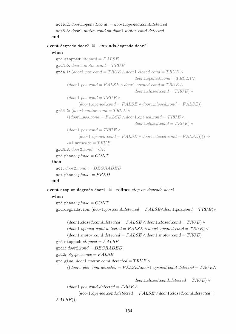
act5 2: door1 opened cond := door1 opened cond detected

act5 3: door1 motor cond := door1 motor cond detected

end

event degrade door2 = extends degrade door2

when

grd stopped: stopped = FALSE

grd4 0: door1 motor cond = TRUE

grd4 1: (door1 pos cond = TRUE ∧ door1 closed cond = TRUE ∧door1 opened cond = TRUE) ∨

(door1 pos cond = FALSE ∧ door1 opened cond = TRUE ∧door1 closed cond = TRUE) ∨

(door1 pos cond = TRUE ∧(door1 opened cond = FALSE ∨ door1 closed cond = FALSE))

grd4 2: (door1 motor cond = TRUE ∧((door1 pos cond = FALSE ∧ door1 opened cond = TRUE ∧

door1 closed cond = TRUE) ∨(door1 pos cond = TRUE ∧

(door1 opened cond = FALSE ∨ door1 closed cond = FALSE))))⇒obj presence = TRUE

grd4 3: door2 cond = OK

grd phase: phase = CONT

then

act: door2 cond := DEGRADED

act phase: phase := PRED

end

event stop on degrade door1 = refines stop on degrade door1

when

grd phase: phase = CONT

grd degradation: (door1 pos cond detected = FALSE∧door1 pos cond = TRUE)∨

(door1 closed cond detected = FALSE ∧ door1 closed cond = TRUE) ∨(door1 opened cond detected = FALSE ∧ door1 opened cond = TRUE) ∨(door1 motor cond detected = FALSE ∧ door1 motor cond = TRUE)

grd stopped: stopped = FALSE

grd1: door2 cond = DEGRADED

grd2: obj presence = FALSE

grd glue: door1 motor cond detected = TRUE ∧((door1 pos cond detected = FALSE∧door1 opened cond detected = TRUE∧

door1 closed cond detected = TRUE) ∨(door1 pos cond detected = TRUE ∧

(door1 opened cond detected = FALSE ∨door1 closed cond detected =

FALSE)))

154

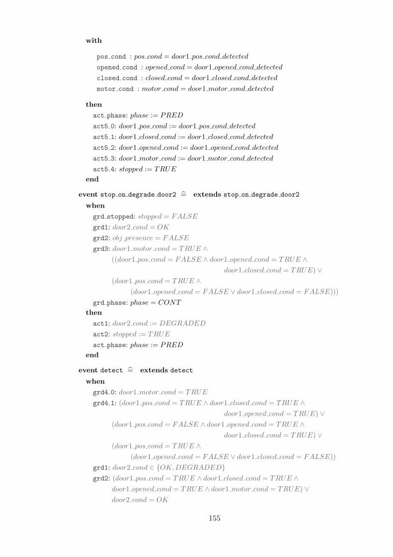
with

pos cond : pos cond = door1 pos cond detected

opened cond : opened cond = door1 opened cond detected

closed cond : closed cond = door1 closed cond detected

motor cond : motor cond = door1 motor cond detected

then

act phase: phase := PRED

act5 0: door1 pos cond := door1 pos cond detected

act5 1: door1 closed cond := door1 closed cond detected

act5 2: door1 opened cond := door1 opened cond detected

act5 3: door1 motor cond := door1 motor cond detected

act5 4: stopped := TRUE

end

event stop on degrade door2 = extends stop on degrade door2

when

grd stopped: stopped = FALSE

grd1: door2 cond = OK

grd2: obj presence = FALSE

grd3: door1 motor cond = TRUE ∧((door1 pos cond = FALSE ∧ door1 opened cond = TRUE ∧

door1 closed cond = TRUE) ∨(door1 pos cond = TRUE ∧

(door1 opened cond = FALSE ∨ door1 closed cond = FALSE)))

grd phase: phase = CONT

then

act1: door2 cond := DEGRADED

act2: stopped := TRUE

act phase: phase := PRED

end

event detect = extends detect

when

grd4 0: door1 motor cond = TRUE

grd4 1: (door1 pos cond = TRUE ∧ door1 closed cond = TRUE ∧door1 opened cond = TRUE) ∨

(door1 pos cond = FALSE ∧ door1 opened cond = TRUE ∧door1 closed cond = TRUE) ∨

(door1 pos cond = TRUE ∧(door1 opened cond = FALSE ∨ door1 closed cond = FALSE))

grd1: door2 cond ∈ OK,DEGRADEDgrd2: (door1 pos cond = TRUE ∧ door1 closed cond = TRUE ∧

door1 opened cond = TRUE ∧ door1 motor cond = TRUE) ∨door2 cond = OK

155

grd5: stopped = FALSE

grd phase: phase = CONT

then

act1: obj presence :∈ BOOL

act phase: phase := PRED

end

event stopped = extends stopped

when

grd: stopped = TRUE

then

skip

end

event object leave = extends object leave

when

grd stopped: stopped = FALSE

grd1: door1 motor cond = TRUE ∧((door1 pos cond = FALSE ∧ door1 opened cond = TRUE ∧

door1 closed cond = TRUE) ∨(door1 pos cond = TRUE ∧

(door1 opened cond = FALSE ∨ door1 closed cond = FALSE)))

grd2: door2 cond = DEGRADED

grd3: obj presence = TRUE

grd phase: phase = CONT

then

act1: obj presence := FALSE

act stopped: stopped := TRUE

act phase: phase := PRED

end

event break2 = extends break2

when

grd4 0: door2 cond 6= BROKEN

grd4 1: ¬(door1 motor cond = FALSE ∨ (door1 pos cond = FALSE ∧(door1 opened cond = FALSE ∨ door1 closed cond = FALSE)))

grd4 3: (door1 motor cond = TRUE ∧((door1 pos cond = FALSE ∧ door1 opened cond = TRUE ∧

door1 closed cond = TRUE) ∨(door1 pos cond = TRUE ∧

(door1 opened cond = FALSE ∨ door1 closed cond = FALSE)))) ∧door2 cond = DEGRADED⇒ obj presence = TRUE

grd5: stopped = FALSE

grd phase: phase = CONT

156

then

act4 1: door2 cond := BROKEN

act4 4: stopped := TRUE

act phase: phase := PRED

end

end

157

Appendix B: AOCS Case Study Model

This appendix contains full Event-B models for the AOCS case study used in Chap-

ter 5 for method evaluation. The development produced a total of 381 proof obliga-

tions, 359 of which were proven automatically, and 22 required interactive proof. A

Rodin project containing the proved models can be found in the Examples section

at [WIFT].

B.1 Context C0

context c0

constants

UNIT ON UNIT OFF GPS COARSE GPS FINE

axioms

axm1: UNIT OFF = 0

axm2: UNIT ON = 1

axm3: GPS COARSE = 1

axm4: GPS FINE = 2

end

B.2 Machine M0

machine m0 sees c0

variables

unitES unitGPS unitPLI

invariants

inv1: unitES ∈ UNIT ON,UNIT OFFinv2: unitGPS ∈ UNIT OFF,GPS COARSE,GPS FINEinv3: unitPLI ∈ UNIT OFF,UNIT ON

events

event INITIALISATION

158

then

act0: unitES := UNIT OFF

act1: unitGPS := UNIT OFF

act2: unitPLI := UNIT OFF

end

event ES work =

when

grd1: unitES = UNIT ON

then

skip

end

event ES switch =

any

newState

where

grd1: newState ∈ UNIT ON,UNIT OFFgrd2: newState 6= unitES

then

act1: unitES := newState

end

event GPS work =

when

grd1: unitGPS ∈ GPS COARSE,GPS FINEthen

skip

end

event GPS switch =

any

newState

where

grd1: newState ∈ UNIT OFF,GPS COARSE,GPS FINEgrd2: newState 6= unitGPS

grd3: unitGPS = UNIT OFF ⇒ newState = GPS COARSE

then

act1: unitGPS := newState

end

event PLI work =

when

grd1: unitPLI = UNIT ON

then

159

skip

end

event PLI switch =

any

newState

where

grd1: newState ∈ UNIT ON,UNIT OFFgrd2: newState 6= unitPLI

then

act1: unitPLI := newState

end

end

B.3 Machine M1

machine m1 refines m0 sees c0

variables

unitES unitGPS unitPLI stopped

invariants

inv stopped: stopped ∈ BOOL

events

event INITIALISATION

extended

then

act0: unitES := UNIT OFF

act1: unitGPS := UNIT OFF

act2: unitPLI := UNIT OFF

act stopped: stopped := FALSE

end

event ES work = extends ES work

when

grd1: unitES = UNIT ON

grd stopped: stopped = FALSE

then

skip

end

event ES switch = extends ES switch

160

any

newStatewhere

grd1: newState ∈ UNIT ON,UNIT OFFgrd2: newState 6= unitES

grd stopped: stopped = FALSE

then

act1: unitES := newState

end

event GPS work = extends GPS work

when

grd1: unitGPS ∈ GPS COARSE,GPS FINEgrd stopped: stopped = FALSE

then

skip

end

event GPS switch = extends GPS switch

any

newStatewhere

grd1: newState ∈ UNIT OFF,GPS COARSE,GPS FINEgrd2: newState 6= unitGPS

grd3: unitGPS = UNIT OFF ⇒ newState = GPS COARSE

grd stopped: stopped = FALSE

then

act1: unitGPS := newState

end

event PLI work = extends PLI work

when

grd1: unitPLI = UNIT ON

grd stopped: stopped = FALSE

then

skip

end

event PLI switch = extends PLI switch

any

newStatewhere

grd1: newState ∈ UNIT ON,UNIT OFFgrd2: newState 6= unitPLI

161

grd stopped: stopped = FALSE

then

act1: unitPLI := newState

end

event stop =

when

grd stopped: stopped = FALSE

then

act stopped: stopped := TRUE

end

event stopped =

when

grd stopped: stopped = TRUE

then

skip

end

end

B.4 Context C2

context c2 extends c0

constants

OFF NOMINAL SCIENCE MODE

axioms

axm1: OFF = 0

axm2: NOMINAL = 1

axm3: SCIENCE = 2

axm4: MODE = 0, 1, 2

end

B.5 Machine M2

machine m2 refines m1 sees c1

variables

unitES unitGPS unitPLI stable mode stopped

162

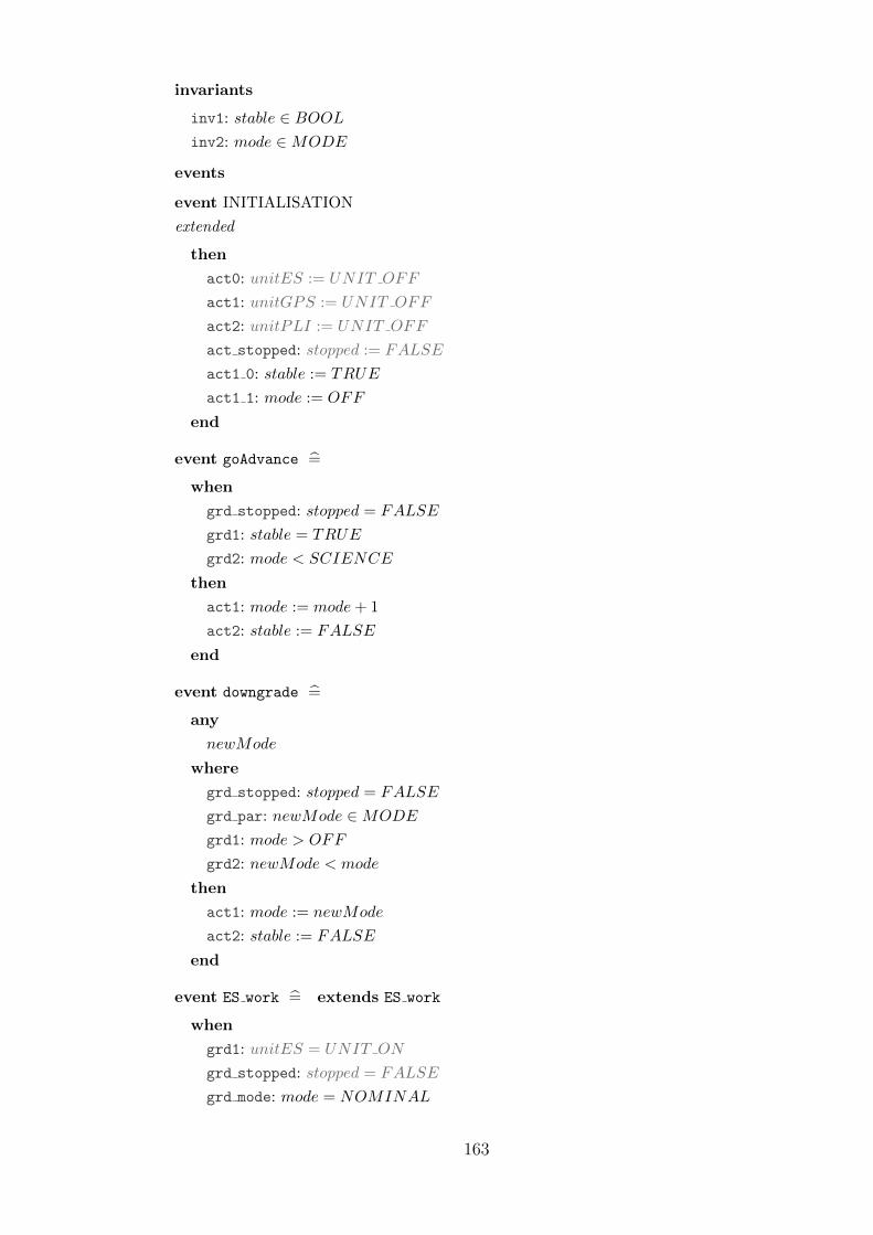
invariants

inv1: stable ∈ BOOL

inv2: mode ∈MODE

events

event INITIALISATION

extended

then

act0: unitES := UNIT OFF

act1: unitGPS := UNIT OFF

act2: unitPLI := UNIT OFF

act stopped: stopped := FALSE

act1 0: stable := TRUE

act1 1: mode := OFF

end

event goAdvance =

when

grd stopped: stopped = FALSE

grd1: stable = TRUE

grd2: mode < SCIENCE

then

act1: mode := mode+ 1

act2: stable := FALSE

end

event downgrade =

any

newMode

where

grd stopped: stopped = FALSE

grd par: newMode ∈MODE

grd1: mode > OFF

grd2: newMode < mode

then

act1: mode := newMode

act2: stable := FALSE

end

event ES work = extends ES work

when

grd1: unitES = UNIT ON

grd stopped: stopped = FALSE

grd mode: mode = NOMINAL

163

then

skip

end

event ES switch on = refines ES switch

when

grd stopped: stopped = FALSE

grd1: unitES = UNIT OFF

grd2: mode = NOMINAL

with

newState : newState = UNIT ON

then

act1: unitES := UNIT ON

end

event ES switch off = refines ES switch

when

grd stopped: stopped = FALSE

grd1: unitES = UNIT ON

grd2: mode ∈ OFF, SCIENCEwith

newState : newState = UNIT OFF

then

act1: unitES := UNIT OFF

end

event GPS work = extends GPS work

when

grd1: unitGPS ∈ GPS COARSE,GPS FINEgrd stopped: stopped = FALSE

grd1 2: mode ∈ NOMINAL, SCIENCEthen

skip

end

event GPS switch on = refines GPS switch

when

grd stopped: stopped = FALSE

grd1: unitGPS < GPS FINE

grd2: mode ∈ NOMINAL, SCIENCEwith

newState : newState = unitGPS + 1

164

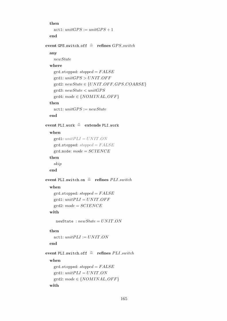
then

act1: unitGPS := unitGPS + 1

end

event GPS switch off = refines GPS switch

any

newState

where

grd stopped: stopped = FALSE

grd1: unitGPS > UNIT OFF

grd2: newState ∈ UNIT OFF,GPS COARSEgrd3: newState < unitGPS

grd4: mode ∈ NOMINAL,OFFthen

act1: unitGPS := newState

end

event PLI work = extends PLI work

when

grd1: unitPLI = UNIT ON

grd stopped: stopped = FALSE

grd mode: mode = SCIENCE

then

skip

end

event PLI switch on = refines PLI switch

when

grd stopped: stopped = FALSE

grd1: unitPLI = UNIT OFF

grd2: mode = SCIENCE

with

newState : newState = UNIT ON

then

act1: unitPLI := UNIT ON

end

event PLI switch off = refines PLI switch

when

grd stopped: stopped = FALSE

grd1: unitPLI = UNIT ON

grd2: mode ∈ NOMINAL,OFFwith

165

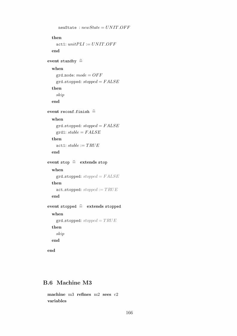
newState : newState = UNIT OFF

then

act1: unitPLI := UNIT OFF

end

event standby =

when

grd mode: mode = OFF

grd stopped: stopped = FALSE

then

skip

end

event reconf finish =

when

grd stopped: stopped = FALSE

grd1: stable = FALSE

then

act1: stable := TRUE

end

event stop = extends stop

when

grd stopped: stopped = FALSE

then

act stopped: stopped := TRUE

end

event stopped = extends stopped

when

grd stopped: stopped = TRUE

then

skip

end

end

B.6 Machine M3

machine m3 refines m2 sees c2

variables

166

unitES unitGPS unitPLI mode stable stopped

invariants

inv modes1: mode = OFF ∧ stable = TRUE⇒unitES = UNIT OFF ∧ unitGPS = UNIT OFF ∧ unitPLI = UNIT OFF

inv modes2: mode = NOMINAL ∧ stable = TRUE⇒unitES = UNIT ON ∧unitGPS = GPS COARSE ∧unitPLI = UNIT OFF

inv modes3: mode = SCIENCE ∧ stable = TRUE⇒unitES = UNIT OFF ∧ unitGPS = GPS FINE ∧ unitPLI = UNIT ON

inv modes4: unitES = UNIT ON ∨ unitGPS ∈ GPS FINE,GPS COARSE ∨unitPLI = UNIT ON ⇒¬(stable = TRUE ∧mode = OFF )

events

event INITIALISATION

extended

then

act0: unitES := UNIT OFF

act1: unitGPS := UNIT OFF

act2: unitPLI := UNIT OFF

act stopped: stopped := FALSE

act1 0: stable := TRUE

act1 1: mode := OFF

end

event goAdvance = extends goAdvance

when

grd stopped: stopped = FALSE

grd1: stable = TRUE

grd2: mode < SCIENCE

then

act1: mode := mode+ 1

act2: stable := FALSE

end

event downgrade = extends downgrade

any

newModewhere

grd stopped: stopped = FALSE

grd par: newMode ∈MODE

grd1: mode > OFF

grd2: newMode < mode

then

act1: mode := newMode

act2: stable := FALSE

167

end

event ES work = extends ES work

when

grd1: unitES = UNIT ON

grd stopped: stopped = FALSE

grd mode: mode = NOMINAL

then

skip

end

event standby = extends standby

when

grd mode: mode = OFF

grd stopped: stopped = FALSE

then

skip

end

event ES switch on = extends ES switch on

when

grd stopped: stopped = FALSE

grd1: unitES = UNIT OFF

grd2: mode = NOMINAL

grd2 0: stable = FALSE

then

act1: unitES := UNIT ON

end

event ES switch off = extends ES switch off

when

grd stopped: stopped = FALSE

grd1: unitES = UNIT ON

grd2: mode ∈ OFF, SCIENCEgrd2 0: stable = FALSE

then

act1: unitES := UNIT OFF

end

event GPS work = extends GPS work

when

grd1: unitGPS ∈ GPS COARSE,GPS FINEgrd stopped: stopped = FALSE

grd1 2: mode ∈ NOMINAL, SCIENCEthen

168

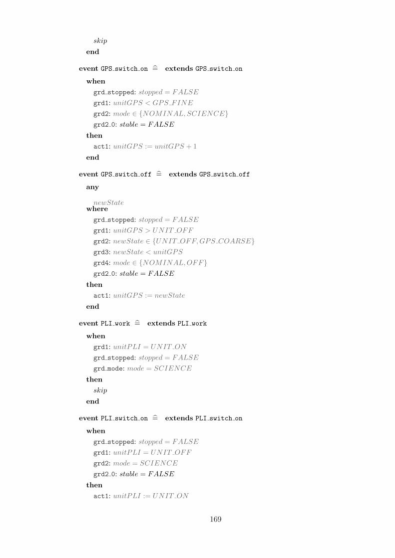
skip

end

event GPS switch on = extends GPS switch on

when

grd stopped: stopped = FALSE

grd1: unitGPS < GPS FINE

grd2: mode ∈ NOMINAL, SCIENCEgrd2 0: stable = FALSE

then

act1: unitGPS := unitGPS + 1

end

event GPS switch off = extends GPS switch off

any

newStatewhere

grd stopped: stopped = FALSE

grd1: unitGPS > UNIT OFF

grd2: newState ∈ UNIT OFF,GPS COARSEgrd3: newState < unitGPS

grd4: mode ∈ NOMINAL,OFFgrd2 0: stable = FALSE

then

act1: unitGPS := newState

end

event PLI work = extends PLI work

when

grd1: unitPLI = UNIT ON

grd stopped: stopped = FALSE

grd mode: mode = SCIENCE

then

skip

end

event PLI switch on = extends PLI switch on

when

grd stopped: stopped = FALSE

grd1: unitPLI = UNIT OFF

grd2: mode = SCIENCE

grd2 0: stable = FALSE

then

act1: unitPLI := UNIT ON

169

end

event PLI switch off = extends PLI switch off

when

grd stopped: stopped = FALSE

grd1: unitPLI = UNIT ON

grd2: mode ∈ NOMINAL,OFFgrd2 0: stable = FALSE

then

act1: unitPLI := UNIT OFF

end

event reconf finish = extends reconf finish

when

grd stopped: stopped = FALSE

grd1: stable = FALSE

grd mode off: mode = OFF ⇒unitES = UNIT OFF ∧unitGPS = UNIT OFF ∧unitPLI = UNIT OFF

grd mode nominal: mode = NOMINAL⇒unitES = UNIT ON∧unitGPS = GPS COARSE∧unitPLI = UNIT OFF

grd mode science: mode = SCIENCE⇒unitES = UNIT OFF ∧ unitGPS = GPS FINE ∧ unitPLI = UNIT ON

then

act1: stable := TRUE

end

event stop = extends stop

when

grd stopped: stopped = FALSE

grd units: unitES = UNIT ON ∨ unitGPS ∈ GPS FINE,GPS COARSE ∨unitPLI = UNIT ON

then

act stopped: stopped := TRUE

end

event stopped = extends stopped

when

grd stopped: stopped = TRUE

then

skip

end

end

170

B.7 Machine M4

machine m4 refines m3 sees c2

variables

unitES unitGPS unitPLI mode stable unitES cond unitGPS cond unitPLI cond stopped

invariants

inv ES cond: unitES cond ∈ 0, 1, 2inv GPS cond: unitGPS cond ∈ 0, 1, 2inv PLI cond: unitPLI cond ∈ 0, 1, 2inv unitPLI cond mode: unitPLI cond = 0 ∧ unitES cond > 0 ∧

unitGPS cond > 0⇒mode ∈ OFF,NOMINALinv units2: mode = NOMINAL ∧ stopped = FALSE⇒

unitES cond > 0 ∧ unitGPS cond > 0

inv units3: mode = SCIENCE ∧ stopped = FALSE⇒unitES cond > 0 ∧ unitGPS cond > 0 ∧ unitPLI cond > 0

inv glue: stopped = TRUE⇔ unitES cond = 0 ∨ unitGPS cond = 0

inv glue1: stopped = FALSE⇔ unitES cond > 0 ∧ unitGPS cond > 0

events

event INITIALISATION

extended

then

act0: unitES := UNIT OFF

act1: unitGPS := UNIT OFF

act2: unitPLI := UNIT OFF

act stopped: stopped := FALSE

act1 0: stable := TRUE

act1 1: mode := OFF

act3 0: unitES cond := 2

act3 1: unitGPS cond := 2

act3 2: unitPLI cond := 2

end

event goAdvance = extends goAdvance

when

grd stopped: stopped = FALSE

grd1: stable = TRUE

grd2: mode < SCIENCE

inv nominal: mode+ 1 = NOMINAL⇒unitES cond > 0 ∧ unitGPS cond > 0

inv science: mode+ 1 = SCIENCE⇒unitES cond > 0 ∧ unitGPS cond > 0 ∧ unitPLI cond > 0

then

171

act1: mode := mode+ 1

act2: stable := FALSE

end

event ES break = refines stop

when

grd1: unitES cond = 1

grd2: unitES = UNIT ON

grd3: unitGPS cond > 0

then

act1: unitES cond := 0

act2: stopped := TRUE

end

event GPS break = refines stop

when

grd1: unitGPS cond = 1

grd2: unitGPS ∈ GPS COARSE,GPS FINEgrd3: unitES cond > 0

then

act1: unitGPS cond := 0

act2: stopped := TRUE

end

event ES work = extends ES work

when

grd1: unitES = UNIT ON

grd stopped: stopped = FALSE

grd mode: mode = NOMINAL

grd3 0: unitES cond > 0

then

skip

end

event standby = extends standby

when

grd mode: mode = OFF

grd stopped: stopped = FALSE

grd1: unitES cond > 0 ∧ unitGPS cond > 0

then

skip

end

event ES switch on = extends ES switch on

when

172

grd stopped: stopped = FALSE

grd1: unitES = UNIT OFF

grd2: mode = NOMINAL

grd2 0: stable = FALSE

grd3 0: unitES cond > 0

then

act1: unitES := UNIT ON

end

event ES switch off = extends ES switch off

when

grd stopped: stopped = FALSE

grd1: unitES = UNIT ON

grd2: mode ∈ OFF, SCIENCEgrd2 0: stable = FALSE

then

act1: unitES := UNIT OFF

end

event GPS work = extends GPS work

when

grd1: unitGPS ∈ GPS COARSE,GPS FINEgrd stopped: stopped = FALSE

grd1 2: mode ∈ NOMINAL, SCIENCEgrd3 0: unitGPS cond > 0

then

skip

end

event GPS switch on = extends GPS switch on

when

grd stopped: stopped = FALSE

grd1: unitGPS < GPS FINE

grd2: mode ∈ NOMINAL, SCIENCEgrd2 0: stable = FALSE

grd3 0: unitGPS cond > 0

then

act1: unitGPS := unitGPS + 1

end

event GPS switch off = extends GPS switch off

any

newStatewhere

173

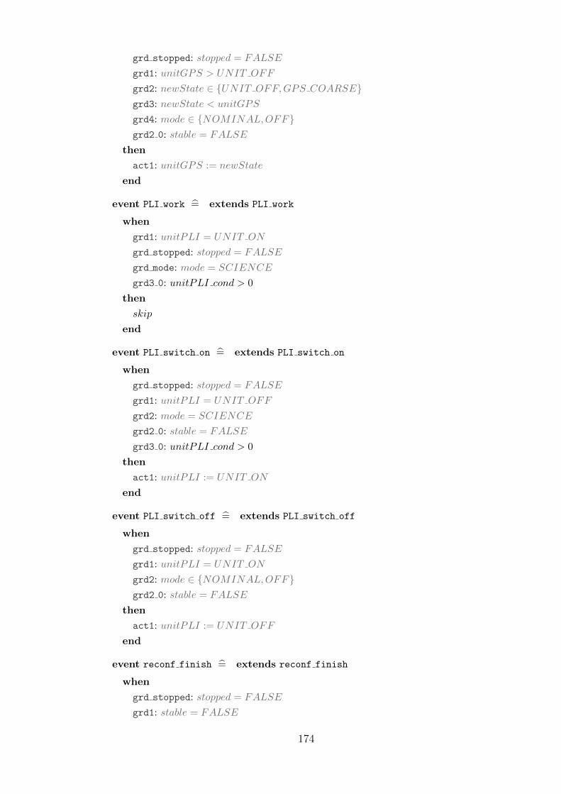
grd stopped: stopped = FALSE

grd1: unitGPS > UNIT OFF

grd2: newState ∈ UNIT OFF,GPS COARSEgrd3: newState < unitGPS

grd4: mode ∈ NOMINAL,OFFgrd2 0: stable = FALSE

then

act1: unitGPS := newState

end

event PLI work = extends PLI work

when

grd1: unitPLI = UNIT ON

grd stopped: stopped = FALSE

grd mode: mode = SCIENCE

grd3 0: unitPLI cond > 0

then

skip

end

event PLI switch on = extends PLI switch on

when

grd stopped: stopped = FALSE

grd1: unitPLI = UNIT OFF

grd2: mode = SCIENCE

grd2 0: stable = FALSE

grd3 0: unitPLI cond > 0

then

act1: unitPLI := UNIT ON

end

event PLI switch off = extends PLI switch off

when

grd stopped: stopped = FALSE

grd1: unitPLI = UNIT ON

grd2: mode ∈ NOMINAL,OFFgrd2 0: stable = FALSE

then

act1: unitPLI := UNIT OFF

end

event reconf finish = extends reconf finish

when

grd stopped: stopped = FALSE

grd1: stable = FALSE

174

grd mode off: mode = OFF ⇒unitES = UNIT OFF ∧unitGPS = UNIT OFF ∧unitPLI = UNIT OFF

grd mode nominal: mode = NOMINAL⇒unitES = UNIT ON∧unitGPS = GPS COARSE∧unitPLI = UNIT OFF

grd mode science: mode = SCIENCE⇒unitES = UNIT OFF ∧ unitGPS = GPS FINE ∧ unitPLI = UNIT ON

then

act1: stable := TRUE

end

event stopped = extends stopped

when

grd stopped: stopped = TRUE

then

skip

end

event ES downgrade = refines downgrade

when

grd1: mode > OFF

grd2: unitES = UNIT ON

grd3: unitES cond = 2

grd4: unitGPS cond > 0

with

newMode : newMode = OFF

then

act1: mode := OFF

act2: stable := FALSE

act3: unitES cond := 1

end

event GPS downgrade = refines downgrade

when

grd1: mode > OFF

grd2: unitGPS > UNIT OFF

grd3: unitGPS cond = 2

grd4: unitES cond > 0

with

newMode : newMode = OFF

then

act1: mode := OFF

act2: stable := FALSE

175

act3: unitGPS cond := 1

end

event PLI downgrade = refines downgrade

when

grd1: mode = SCIENCE

grd2: unitPLI = UNIT ON

grd3: unitPLI cond = 2

grd4: unitES cond > 0 ∧ unitGPS cond > 0

with

newMode : newMode = NOMINAL

then

act1: mode := NOMINAL

act2: stable := FALSE

act3: unitPLI cond := 1

end

event PLI break = refines downgrade

when

grd1: mode = SCIENCE

grd2: unitPLI = UNIT ON

grd3: unitPLI cond = 1

grd4: unitES cond > 0 ∧ unitGPS cond > 0

with

newMode : newMode = NOMINAL

then

act1: mode := NOMINAL

act2: stable := FALSE

act3: unitPLI cond := 0

end

end

176