Embed Size (px)
Citation preview
IJRRAS 42 (1) ● Jan 2020 www.arpapress.com/Volumes/Vol42Issue1/IJRRAS_42_1_04.pdf
36
A METHOD FOR TRANSIENT HEAT CONDUCTION
Jian Song*, Lili Yan and Yingying Yin
School of Mathematics and Statistics, Shandong University of Technology, Zibo 255049, China
ABSTRACT
In this paper, we proposed a calculation method which combining radial basis function method and Houbolt method
to solve the transient heat conduction problem. Houbolt method is used for discrete differences in time domain. In
order to reduce the influence of shape parameter, this study proposed an improved radial basis function, and the
improved radial basis function is used to compute the value of the problem. This method is accurate and stable, and
it can solve the transient heat conduction problem excellently. Finally, three numerical examples are applied to
illustrate the effectiveness of the proposed method.
Key words: transient heat conduction, radial basis function, Houbolt method.
1. INTRODUCTION
It is difficult to solve the transient heat conduction because of its inherent complexity. But with the development of
science and technology, there are more and more solutions to solve this problem, for example, the finite element
method (FEM)[1], boundary element method (BEM)[2-4], the finite difference method (FDM), and meshfree
method[9-15] have been well displayed in recent years and have been frequently used in heat conduction problems.
All these methods display different advantages and disadvantages. BEM has a distinct advantage is its property in
reducing the dimensionality of heat conduction problem by one when compare with FDM and FEM. However, the
obvious advantage is gradually disappearing when this method is used in solving transient and non-homogeneous
problems. Meshfree method is used in interpolating the field function by the fitting function, and it ensures the high-
order continuity of the basic field variables either in the entire computation domain or on the computation boundary.
In recent years, mesh-free multiquadric radial basis functions (MQ-RBFs) method which developed by Kansa [5]
has attracted the attention of the researchers since it is easy to calculation and has higher precision. However, it has a
disadvantage that can not be ignored: it is seriously affected by shape parameters.
In this paper, we propose a combine method based on RBFs[6] and Houbolt method, which overcome the sensitivity
of parameter and get excellent precision.
Section two introduces the governing equation of the transient heat conduction. Section three presentation the
combine method and the improved RBF. In order to prove its performance, section four test three numerical
examples. And in section five, we summarize the advantages and disadvantages of the method in this paper.
2. GOVERNING EQUATION
Assuming that the computed domain of the transient heat conduction is which bounded by 21 =, where
21, are the temperature boundary, the heat flux boundary respectively. The governing equation of the problem is
( ) ( ) ( ) ( )
t
tucfukuktfuk
=++=+
),(, 2 x
xxx , in (1)
where2 is the Laplace operator,
ft,are time and heat source, respectively,
, k , c denotes mass density,
thermal conductivity, and specific heat respectively, and may vary with ( )21, xx=x
.
The boundary condition can be written as follows:
),(),( tutu xx = on 1 (2a)
),(),( tqtq xx = on 2 (2b)
and initial condition
)(),( 00 xx utu = in (3)
where u ,q
are specified value of temperature on 1 and the given heat flux on 2 , respectively. And
n
ukukq
=−= n
, ( )21,nn=n
is the outward unit normal to the boundary.
IJRRAS 42 (1) ● Jan 2020 Song et al. ● A Method for Transient Heat Conduction
37
3. SOLVING THE TRANSIENT HEAD CONDUCTION WITH A COMBINE METHOD
3.1 the combine method
In order to solve the time-dependent terms, we use the following method which is in Ref [7] to discretize the time
domain: 1
1 1 21(11 18 9 2 )
6
n
n n n nuu u u u
t t
+
+ − − − + −
, (4)
and when 2n ,
1
11( )
n
n nuu u
t t
+
+ −
, where t is the time step, 1
1( , )n
nu u t+
+= x, 1n nt t t n t t+ = + = +
By using Eq(4) into Eq(1), we can obtain the following equation:
( ) ( )2 1 1 1 1 2 11 1( 18 9 2 )
6 6
n n n n n n nk u k u u c u u u ft t
+ + + − − + + − = − + − +
x x
( ) ( )2 1 1 1 11 1n n n n nk u k u u c u ft t
+ + + + + − = +
x x
and we can use Radial basis function method to solve nu .
We assumed that RRd →:
is a continunous mapping and 0)0(
, then a Radial basis function on dR is
)(r,where ir xx−=
. If N points NiRd
i ,1, =x are closed in
dR , then
+1 +1
1
( , ) ( )N
n n
i i
i
u u t r=
= =x
(5)
also can be called a radial basis function. Radial basis functions can be divided into two categories. The first
category is infinitely differentiable and seriously affected by shape parameters c .The second category is not
infinitely differentiable and is not affected by shape parameters c , but has poor accuracy. In this paper, we focus on
the first category.
Eq(5) also can be written as the form:
+1
1
( , ) ( , ) ( )N
n n
i i
i
f t Lu t r=
= =x x
(6)
where L is a linear operator,)()( ii r xx −=
, and i is a set of undetermined coefficients, and 1( , )nf t +x
is
a known function. If we choose N collocation points, then Eq(6) can be written as
+1
1
( , ) ( , ) ( )N
n n
j j i i j
i
f t Lu t r=
= =x x
therefore, we define
= )(rψy (7)
where T
n ],,,[ 21 =,
=
)()()(
)()()(
)()()(
)(
21
22221
11211
NNNN
N
N
rrr
rrr
rrr
r
ψ
,
ijjr xx −=.
By the Eq(7), the governing equation and boundary condition can be transformed into the following form: +1 +1( , ) ( , )n nLu t f t=x x , x
+1 +1( , ) ( , )n nGu t g t=x x , x
where, GL, are linear operator. The above equations produce a system of linear equations:
BA = where
IJRRAS 42 (1) ● Jan 2020 Song et al. ● A Method for Transient Heat Conduction
38
−
−=
))((
))((
ij
ij
xxG
xxL
A
,
ij
ij
xx
xx
,
,
+1
+1
( , )
( , )
n
n
f t
g t
=
xB
x
3.2 An improved RBF
Some well-known RBFs has been proposed already, for example, Multiquadratic RBF(MQ-RBF), Inverse
multiquadratic RBF(IMQ-RBF,), Gaussian RBF(GA-RBF), and Inverse quadratic RBF, but, usually, the RBFs
generated by them often have an fatal flaw: heavily influenced by shape parameters c . Then we use the improved
RBF to avoid the influence of shape parameters [7]:
=)(rj
2
5
1ln( ( ))
1
2 2
j
j
c r fcf r
r
+
+ +
where 2 2 2( ) ( )j jr x x y y= − + −
,
22 crf j +=.
In order to verify the effectiveness of the proposed method, we have tried the following three numerical experiments
4. NUMERICAL EXAMPLE
In this section, in order to make comparison with the exact solution, we set the root mean square( RMSE ) as
follows:
N
II
RMSE
n
i
numexa=
−
= 1
2)(
where exaI and numI
are obtained by exact and numerical solution, N is the number of center points.
Example 1. Consider the problem in Ref [6]:
0u
u ft
+ − =
,
the computational domain is[0,1] [0,1]
, the source term as follows:
1 2sin( )sin( )(2sin( ) cos( ))f x x t t= +
The analytical solution is given by 1 2sin( )sin( )sin( )u x x t=, thus we can obtain the boundary condition and initial
condition.
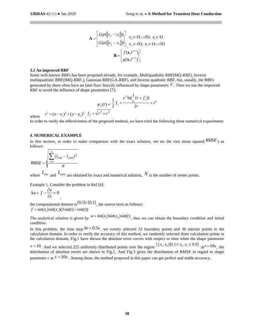
In this problem, the time step 0.5t s = , we evenly selected 32 boundary points and 36 interior points in the
calculation domain. In order to verify the accuracy of this method, we randomly selected three calculation points in
the calculation domain, Fig.1 have shown the absolute error curves with respect to time when the shape parameter
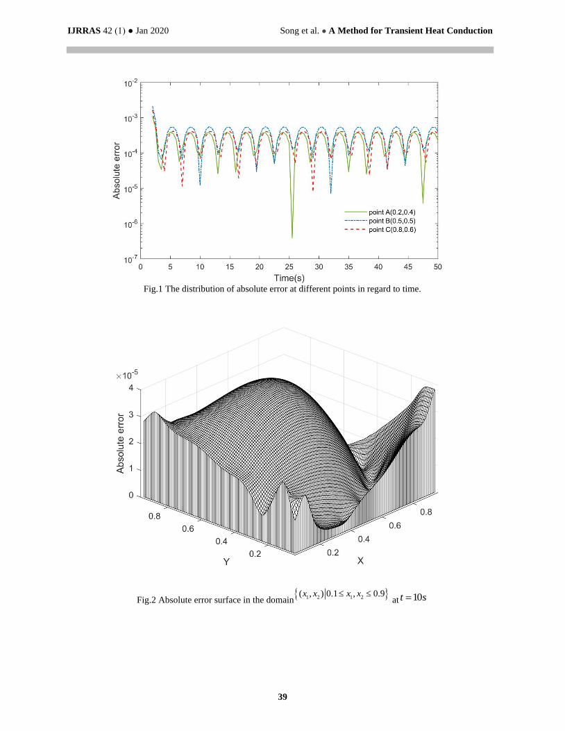
10c = . And we selected 225 uniformly distributed points over the region 1 2 1 2( , ) 0.1 , 0.9x x x x
at 10t s= , the
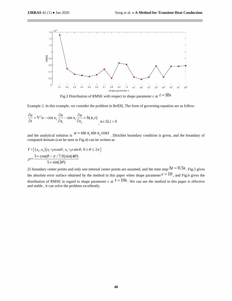
distribution of absolute errors are shown in Fig.2. And Fig.3 gives the distribution of RMSE in regard to shape
parameter c at 10t s= . Among them, the method proposed in this paper can get perfect and stable accuracy.
IJRRAS 42 (1) ● Jan 2020 Song et al. ● A Method for Transient Heat Conduction
39
Fig.1 The distribution of absolute error at different points in regard to time.
Fig.2 Absolute error surface in the domain 1 2 1 2( , ) 0.1 , 0.9x x x x
at 10t s=
IJRRAS 42 (1) ● Jan 2020 Song et al. ● A Method for Transient Heat Conduction
40
Fig.3 Distribution of RMSE with respect to shape parameter c at 10t s=
Example 2. In this example, we consider the problem in Ref[8], The form of governing equation are as follow:
2
2 1
1 2
cos sin ( , )u u u
u x x h tt x x
= − − +
x
,, 0t x
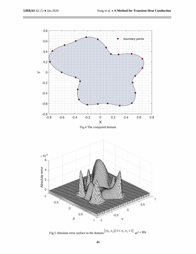
and the analytical solution is 1 2sin sin cosu x x t=. Dirichlet boundary condition is given, and the boundary of
computed domain (can be seen in Fig.4) can be written as
1 2 1 2= ( , ) = cos , = sin , 0 2x x x x
3 cos( / 7.0)sin(4 )=
5 sin(2 )
+ −
+
25 boundary center points and only one internal center points are assumed, and the time step 0.5t s = . Fig.5 gives
the absolute error surface obtained by the method in this paper when shape parameter 10c = , and Fig.6 gives the
distribution of RMSE in regard to shape parameter c at 10t s= . We can see the method in this paper is effective
and stable , it can solve the problem excellently.
IJRRAS 42 (1) ● Jan 2020 Song et al. ● A Method for Transient Heat Conduction
41
Fig.4 The computed domain
Fig.5 Absolute error surface in the domain 1 2 1 2( , ) -1 , 1x x x x
at 10t s=
IJRRAS 42 (1) ● Jan 2020 Song et al. ● A Method for Transient Heat Conduction
42
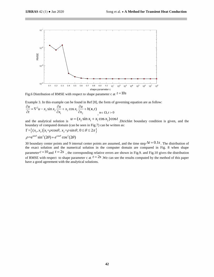
Fig.6 Distribution of RMSE with respect to shape parameter c at 10t s=
Example 3. In this example can be found in Ref [8], the form of governing equation are as follow:
2
2 2 2 1
1 2
sin cos ( , )u u u
u x x x x h tt x x
= − + +
x
, , 0t x
and the analytical solution is 2 1 1 2( sin cos )cosu x x x x t= +.Dirichlet boundary condition is given, and the
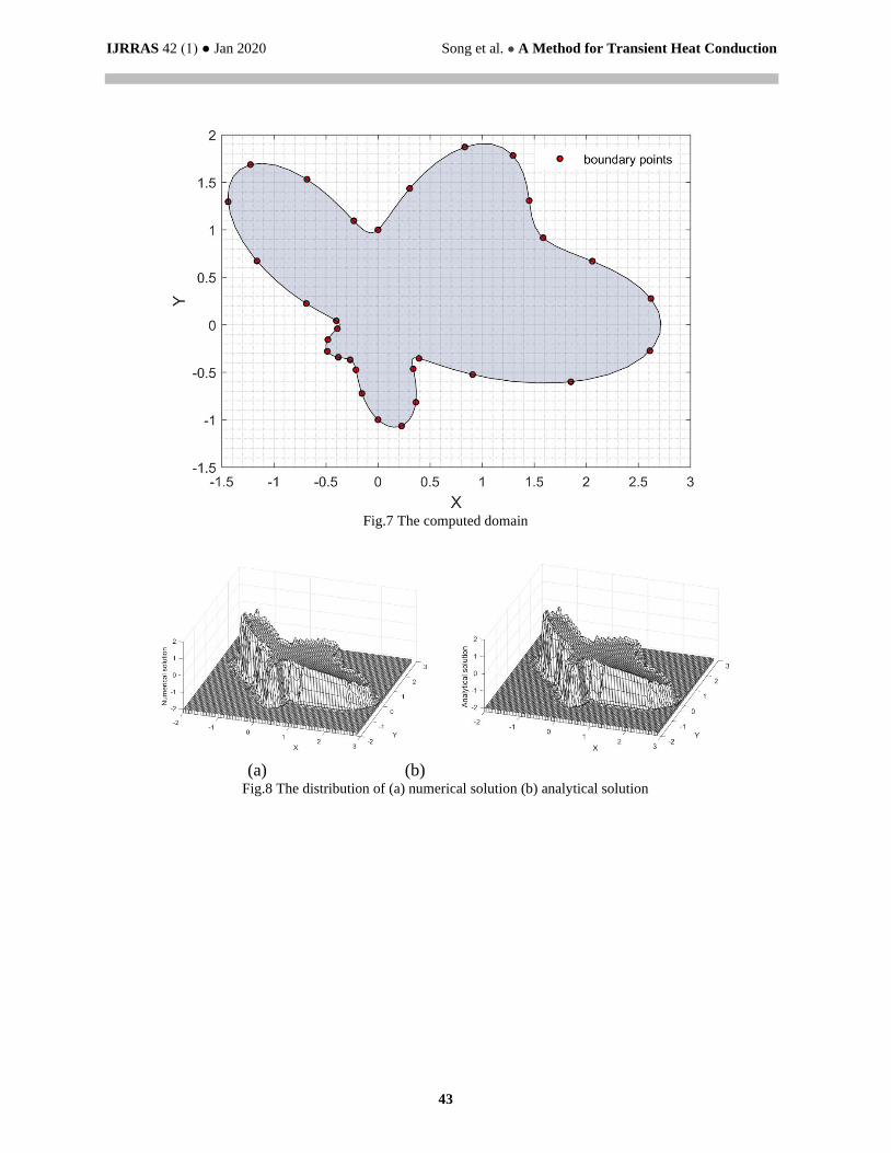
boundary of computed domain (can be seen in Fig.7) can be written as:
1 2 1 2= ( , ) = cos , = sin , 0 2x x x x
sin 2 cos 2=e sin (2 ) cos (2 )e +
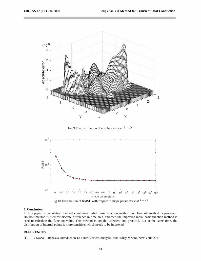
30 boundary center points and 9 internal center points are assumed, and the time step 0.1t s = . The distribution of
the exact solution and the numerical solution in the computer domain are compared in Fig. 8 when shape
parameter 10c = and 2t s= , the corresponding relative errors are shown in Fig.9. and Fig.10 gives the distribution
of RMSE with respect to shape parameter c at 2t s= .We can see the results computed by the method of this paper
have a good agreement with the analytical solutions.
IJRRAS 42 (1) ● Jan 2020 Song et al. ● A Method for Transient Heat Conduction
43
Fig.7 The computed domain
(a) (b)
Fig.8 The distribution of (a) numerical solution (b) analytical solution
IJRRAS 42 (1) ● Jan 2020 Song et al. ● A Method for Transient Heat Conduction
44
Fig.9 The distribution of absolute error at 2t s=
Fig.10 Distribution of RMSE with respect to shape parameter c at 2t s=
5. Conclusion
In this paper, a calculation method combining radial basis function method and Houbolt method is proposed.
Houbolt method is used for discrete difference in time area, and then the improved radial basis function method is
used to calculate the function value. This method is simple, effective and practical. But at the same time, the
distribution of internal points is more sensitive, which needs to be improved.
REFERENCES
[1]. B. Szabó, I. Babuška, Introduction To Finite Element Analysis, John Wiley & Sons, New York, 2011.
IJRRAS 42 (1) ● Jan 2020 Song et al. ● A Method for Transient Heat Conduction
45
[2]. A.H.D. Cheng, D.T. Cheng, Heritage and early history of the boundary element method, Eng. Anal. Bound. Elem.
29 (3) (2005) 268–302.
[3]. C.A. Brebbia, J.C.F. Telles, L.C. Wrobel, Boundary Element Techniques: Theory and Application in Engineering,
Springer, Berlin, 1984.
[4]. P.K. Banerjee, The Boundary Element Methods in Engineering, McGRAW-HILL Book Company, Europe, 1994.
[5]. H. Wang , Q-H. Qin , Y-L. Kang. A meshless model for transient heat conduction in functionally graded materials,
Comput Mech (2006) 38: 51–60.
[6]. S. Kazem , J.A. Rad. Radial basis functions method for solving of a non-local boundary value problem with
Neumann’s boundary conditions. Applied Mathematical Modelling 36 (2012) 2360–2369
[7]. Ji Lin, Wen Chen, C.S. Chen, A new scheme for the solution of reaction diffusion and wave propagation problems,
Applied Mathematical Modelling 38 (2014) 5651–5664.
[8]. Yaoming Zhang, An accurate and stable RBF method for solving partial differential equations, Applied
Mathematics Letters 97 (2019) 93–98.
[9]. Z.C. Li, T.T. Lu, H.Y. Hu, A. Cheng, Trefftz and Collocation Methods, WIT Press, 2008.
[10]. G.R. Liu, Meshfree Methods: Moving Beyond the Finite Element Method, second ed., CRC Press, BocaRaton,
2009.
[11]. S.N. Atluri, The Meshless Method(MLPG) for Domain & BIE Discretizations, Tech. Science Press, California,
2004.
[12]. Y.X. Mukherjee, S. Mukherjee, Boundary Methods: Elements, Contours, and Nodes, CRC Press, Boca Raton,
2005.
[13]. J.M. Zhang, X.Y. Qin, X. Han, G.Y. Li, A boundary face method for potential problems in three dimensions,
Internat. J. Numer. Methods Engrg. 80 (2009)320–337.
[14]. X.L. Li, A meshless interpolating Galerkin boundary node method for Stokes flows, Eng. Anal. Bound. Elem. 51
(2015) 112–122.
[15]. K.M. Liew, Y.M. Cheng, S. Kitipornchai, Boundary element-free method (BEFM) and its application to two-
dimensional elasticity problems, Internat. J.Numer. Methods Engrg. 65 (2006) 1310–1332.


![Chapter 3: Unsteady State [ Transient ] Heat Conduction](https://img.pdfslide.net/doc/110x75/5681626f550346895dd2dd81/chapter-3-unsteady-state-transient-heat-conduction.jpg)