A method to improve Standard PSO

A method to improve Standard PSO

Technical report. DRAFT MC2009-03-13

Maurice Clerc

Abstract

In this report, I present my personal method to design a more accurate version of PSO, assuming we know what kind of

problems we will have to solve. To illustrate the method, I consider a class of problems that are moderately multimodal

and not of very high dimensionality (typically smaller than 30). The starting version is Standard PSO 2007 (SPSO 07).

A modi�ed velocity update equation is used, speci�c to the considered class of problems. Then, in order to improve the

robustness of the algorithm, more general modi�cations are added (in particular, better initialisations, and the use of two

kind of particles). On the whole, the resulting algorithm is indeed an improvement of SPSO 07, though the improvement

is not always very impressive. In passing, I give a precise de�nition of �better than�, and explain why the classical �mean

best� performance criterion may easily be completely meaningless.

1 Why this paper?

A question I often face is this: �You are always referring to Standard PSO 2007 (SPSO 07, [1]). Isn't it possibleto design a better version?�. The answer is of course �yes�. It is even written in the source code available online:

�This PSO version does not intend to be the best one on the market�

On the one hand, it is indeed not very di�cult to write a better PSO. On the other hand, as a reviewer I read alot of papers in which the authors claim they have succeeded in doing that, though it is not really true., mainlyfor two reasons:

• they start from a bad version of PSO (usually a �global best� one). Although they may really improve it,the resulting algorithm is still not as good as SPSO 07.

• or they start from a reasonably good version (or even from SPSO 07 itself), but they update it havingapparently no clear idea of what the modi�cation is for. A typical example is the usual claim �we want toimprove the exploitation/exploration balance� without giving any rigorous de�nition of what this balanceis. As a result, the modi�ed algorithm may or may not be better, more or less in a random way, and wedo no event know why.

Also, of course, there is the well known problem of comparison of two algorithms. Often, we �nd something like�our new algorithm B is therefore better than algorithm A� ... without any clear de�nition of �better than�. Letus �rst say a few words about this point.

2 My algorithm is better than yours

What does such a claim mean? First, such a claim is valid only if we agree on a common benchmark. Let us say,for example, we consider a subset of the CEC 2005 benchmark [2]. Then, we have to agree on a given criterion.For example for each function, the criterion may be Cr = �success rate over N runs, for a given accuracy ε,after at most F �tness evaluations for each run, or, in case of a tile, mean of the best results�. Note that thecriterion may be a probabilistic one (for example Cr′= �the probability that A is better than B on this problem

1

3 STEP 1: A SMALL �REPRESENTATIVE� BENCHMARK

according to the criterion Cr is greater than 0.5�). What is important is to clearly de�ne the meaning of �Ais better than B on one problem�. A lot of researchers indeed use such an approach, and then perform nicestatistical analyses (null hypothesis, p-test, and so on), in order to decide �in probability� whether an algorithmA is better than an algorithm B, on the whole benchmark.

However, in the process, they miss a simple and frustrating fact: there is no complete order in RD, forall D > 1. Why is that important? It may be useful to express it more formally. Let us say the benchmarkcontains P problems. We build two comparison vectors. First CA,B = (cA,B,1, . . . , cA,B,P )with cA,B,i = 1 ifA is better than B on problem i (according to the unique criterion de�ned), cA,B,i = 0 otherwise. SecondCB,A = (cB,A,1, . . . , cB,A,P ) with cB,A,i = 1 if B is better than A on the problem i, and cB,A,i = 0 otherwise.We have to compare the two numerical vectors CA,B and CB,A. Now, precisely because there is no completeorder in RD, we can say that A is better than B if and only if for any i we have cA,B,i ≥ cB,A,i for all i, and ifthere exists j so that cA,B,j > cB,A,j .

This is similar to the de�nition of the classical Pareto dominance. As we have P values of one criterion,the process of comparing A and B can be seen as a multicriterion (or multiobjective) problem. It implies thatmost of the time no comparison is possible, except by using an aggregation method. For example, here, wecould count the number of 1s in each vector, and say that the one with the larger sum �wins�. But the pointis that any aggregation method is arbitrary, i.e. for each method there is another one that leads to a di�erentconclusion1.

Let us consider an example:

• the benchmark contains 5 unimodal functions f1 to f5, and 5 multimodal ones f6 to f10

• the algorithm A is extremely good on unimodal functions (very easy, say for a gradient method)

• the algorithm B is quite good for multimodal functions, but not for unimodal ones.

You �nd cA,B,i = 1 for i = 1, 2, 3, 4, 5, and also for 6 (just because, for example, the attraction basin of theglobal optimum is very large, compared to the ones of the local optima), and cB,A,i = 1 for i = 7, 8, 9, 10. Yousay then "A is better than B". An user trusts you, and chooses A for his problems. And as most of interestingreal problems are multimodal, he will be very disappointed.

So, we have to be both more modest and more rigorous. That is why the �rst step in our method of designingan �improved PSO� is the choice of a small benchmark. But we will say that A is better than B only if it istrue for all the problems of this benchmark.

3 Step 1: a small �representative� benchmark

This is the most speci�c part of the method, for it is depends on the kind or problems we do want to solve laterwith our �improved PSO�. Let us consider the following class of problems:

• moderately multimodal, or even unimodal (but of course we are not supposed to know it in advance)

• not of too high dimensionality (say no more than 30)

For this class, to which a lot of real problems belong, I have found that a good small benchmark may be thefollowing one (see the table 1):

• CEC 2005 Sphere (unimodal)

• CEC 2005 Rosenbrock (one global optimum, at least one local optimum as soon as the dimension is greaterthan 3)

• Tripod (two local optima, one global optimum, very deceptive [3])

These three functions are supposed to be �representative� of our class of problem. If we have an algorithm thatis good on them, then it is very probably also good for a lot of other problems of the same class. Our aim isthen to design a PSO variant that is better than SPSO 07 for these three functions. Our hope is that this PSOvariant will indeed be also better than SPSO 07 on more problems of the same kind. And if it is true even forsome highly multimodal problems, and/or for higher dimensionality, well, we can consider that as a nice bonus!

1 For example, it is possible to assign a "weight" to each problem (which represents how "important" is this kind of problem forthe user) and to linearly combine the cA,B,i and cB,A,i. But if, for a set of (non identical) weights, A is better than B, then italways exists another one for which B is better than A.

2

5 STEP 3: SELECTING THE RIGHT OPTIONS

Tab. 1: The benchmark. More details are given in 9.1

Search Required Maximum numberspace accuracy of �tness evaluations

CEC 2005 Sphere [−100, 100]30 0.000001 15000

CEC 2005 Rosenbrock [−100, 100]10 0.01 50000

Tripod [−100, 100]2 0.0001 10000

4 Step 2: a highly �exible PSO

My main tool is a PSO version (C code), which is based on SPSO 07. However I have added a lot of options, inorder to have a very �exible research algorithm. Actually, I often modify it, but you always can �nd the latestversion (named Balanced PSO) on my technical site [4]. When I used it for this paper, the main options were:

• two kind of randomness (KISS [5], and the standard randomness provided in LINUX C compiler). Inwhat follows, I always use KISS, so that the results can be more reproducible

• seven initialisation methods for the positions (in particular a variant of the Hammersley's one [6])

• six initialisation methods for the velocities (zero, completely random, random �around� a position, etc.)

• two clamping options for the position (actually, just �clamping like in SPSO 07�, or �no clamping and noevaluation�)

• possibility to de�ne a search space greater than the feasible space. Of course, if a particle �ies outside thefeasible space, its �tness is not evaluated

• six local search options (no local search as in SPSO 07, uniform in the best local area, etc.). Note that itimplies a rigorous de�nition of what a �local area� is. See [7]

• two options for the loop over particles (sequential or at random)

• six strategies

The strategies are related to the classical velocity update formula

v (t+ 1) = wv (t) +R (c1) (p (t)− x (t)) +R (c2) (g (t)− x (t)) (1)

One can use di�erent coe�cients w, and di�erent random distributions R. The most interesting point isthat di�erent particles may have di�erent strategies.

In the C source code, each option has an identi�er to easily describe the options used. For example, PSOP1 V2 means: SPSO 07, in which the initialisation of the positions is done by method 1, and the initialisationof the velocities by the method 2. Please refer to the on line code for more details. In our case, we will now seenow how an interesting PSO variant can be designed by using just three options.

5 Step 3: selecting the right options

First of all, we simulate SPSO 07, by setting the parameters and options to the corresponding ones. The resultsover 500 runs are given in the table 2. In passing, it is worth noting that the usual practice of launching only25 or even 100 runs is not enough, for really bad runs may occur quite rarely. This is obvious for Rosenbrock,as we can see from the table 3. Any conclusion that is drawn after just 100 runs is risky, particularly if youconsider the mean best value. The success rate is more stable. More details about this particular function aregiven in 9.5.

3

5.1 Applying a speci�c improvement method 5 STEP 3: SELECTING THE RIGHT OPTIONS

Tab. 2: Standard PSO 2007. Results over 500 runs

Success rate Mean best

CEC 2005 Sphere 84.8% 10−6

CEC 2005 Rosenbrock 15% 12.36Tripod 46% 0.65

Tab. 3: For Rosenbrock, the mean best value is highly depending on the number of runs (50000 �tness evaluationsfor each run). The success rate is more stable

Runs Success rate Mean best value

100 16% 10.12500 15% 12.361000 14,7% 15579.32000 14% 50885.18

5.1 Applying a speci�c improvement method

When we consider the surfaces of the attraction basins, the result for Tripod is not satisfying (the success rateshould be greater then 50%). What options/parameters could we modify in order to improve the algorithm?Let us call the three attraction basins as B1, B2, and B3 . The problem is deceptive because two of them, sayB2and B3, lead to only local optima. If, for a position x in B1 (i.e. in the basin of the global optimum) theneighbourhood best g is either in B2or in B3, then, according to the equation 1, even if the distance betweenx and g is high, the position x may be easily modi�ed such that it is not in B1any more. This is because inSPSO 07 the term R (c2) (g (t)− x (t))is simply U (0, c2) (g (t)− x (t)), where U is the uniform distribution.

However, we are interested on functions with a small number of local optima, and therefore we may supposethat the distance between two optima is usually not very small. So, in order to avoid the above behaviour, weuse the idea is that the further an informer is, the smaller is its in�uence( this can be seen as a kind of niching).We may then try a R (c2) that is in fact a R (c2, |g − x|), and decreasing with |g − x|. The optional formula Iuse to do that in my ��exible� PSO is

R (c2, |g − x|) = U (0, c2)(

1− |g − x|xmax − xmin

)λ(2)

Experiments suggest that λ should not be too high, because in that case, although the algorithm becomesalmost perfect for Tripod, the result for Sphere becomes quite bad. In practice, λ = 2 seems to be a goodcompromise. With this value the result for Sphere is also improved as we can see from the table 4. Accordingto our nomenclature, this PSO is called PSO R2. The result for Rosenbrock may be now slightly worse, butwe have seen that we do not need to worry too much about the mean best, if the success rate seems correct.Anyway, we may now also apply some �general� improvement options.

Tab. 4: Results with PSO R2 (�distance decreasing� distribution, according to the equation 2


CEC 2005 Sphere 98.6% 0.14× 10−6

CEC 2005 Rosenbrock 13.4% 10.48Tripod 47.6% 0.225

4

6 NOW, LET'S TRY 5.2 Applying some general improvement options (initialisations)

5.2 Applying some general improvement options (initialisations)

The above option was speci�cally chosen in order to improve what seemed to be the worst result, i.e. the one forthe Tripod function. Now, we can trigger some other options that are often bene�cial, at least for moderatelymultimodal problems:

• modi�ed Hammersley method for the initialisation of the positions x

• One-rand method for the initialisation of the velocity of the particle whose initial position is x, i.e.v = U (xmin, xmax)− x. Note that in SPSO 07, the method is the �Half-di�� one, i.e.

v = 0.5 (U (xmin, xmax)− U (xmin, xmax))

This modi�ed algorithm is PSO R2 P2 V1. The results are given in the table 5, and are clearly better than theones of SPSO 07. They are still not completely satisfying (cf. Rosenbrock), though. So, we can try yet anotheroption, which can be called �bi-strategy�.

Tab. 5: Results when applying also di�erent initialisations, for positions and velocities (PSO R2 P2 V1)


CEC 2005 Sphere 98.2% 0.15× 10−6


5.3 Bi-strategy

The basic idea is very simple: we use two kinds of particles. In practice, during the initialisation phase, weassign one of two possible behaviours, with a probability equal to 0.5. These two behaviours are simply:

• the one of SPSO 07. In particular, R (c2) = U (0, c2)

• or the one of PSO R2 (i.e. by using equation 2)

The resulting algorithm is PSO R3 P2 V1. As we can see from the table 6, for all the three functions now weobtain results that are also clearly better than the ones of SPSO 07. Success rates are slightly worse for Sphereand Rosenbrock, slightly better for Tripod, so no clear comparison is possible. However more tests (not detailedhere) show that this variant is more robust, as we can guess by looking at the mean best values, so we keepit. Two questions, though. Is it still valid for di�erent maximum number of �tness evaluations (�search e�ort�).And is it true for more problems, even if they are not really in the same �class�, in particular if they are highlymultimodal? Both answers are a�rmative, as tackled in next sections.

Tab. 6: Results by adding the bi-strategy option (PSO R3 P2 V1)


CEC 2005 Sphere 96.6% < 10−10


6 Now, let's try

6.1 Success rate vs �Search e�ort�

Here, on the same three problems, we simply consider di�erent maximum numbers of �tness evaluations(FEmax), and we evaluate the success rate over 500 runs. As we can see from the �gure 1, for any FEmax the

5

6.2 Moderately multimodal problems 7 CLAIMS AND SUSPICION

success rate of our variant is greater than the one of SPSO 07. SO, we can safely say that it is really better,at least on this small benchmark. Of course, it is not always so obvious. Giving a long list of results is outof the scope of this paper, which is just about a design method, but we can nevertheless have an idea of theperformance on a few more problems.

6.2 Moderately multimodal problems

Table 7 and �gure 2 are about moderately multimodal problems. This is a small selection, to illustrate di�erentcases:

• clear improvement, i.e. no matter what the number of �tness evaluations is, but the improvement is small(Schwefel, Pressure Vessel). Actually SPSO 07 is already pretty good on these problems (for example, forPressure Vessel, SOMA needs more than 50000 �tness evaluations to solve it [8]), so our small modi�cationscan not improve it a lot.

• questionable improvement, i.e. depending on the number of �tness evaluations (Compression spring)

• clear big improvement (Gear train). For this problem, and after 20000 �tness evaluations, not only thesuccess rate of PSO R3 P2 V1 is 92.6%, but it �nds the very good solution (19, 16, 43, 49) (or an equivalentpermutation), 85 times over 500 runs. The �tness of this solution is 2.7×10−12(SOMA needs about 200,000evaluations to �nd it).

Even when the improvement is not very important, the robustness is increased. For example, for PressureVessel, with 11000 �tness evaluations, the mean best is 28.23 (standard dev. 133.35) with SPSO 07, as it is18.78 (standard dev. 56.97) with PSO R3 P2 V1.

Tab. 7: More moderately multimodal problems. See 9.2 for details

Search Requiredspace accuracy

CEC 2005 Schwefel [−100, 100]10 0.00001Pressure vessel 4 variables 0.00001(discrete form) objective 7197.72893

Compression spring 3 variables 0.000001objective 2.625421

(granularity 0.001 for x3)Gear train 4 variables 10−9

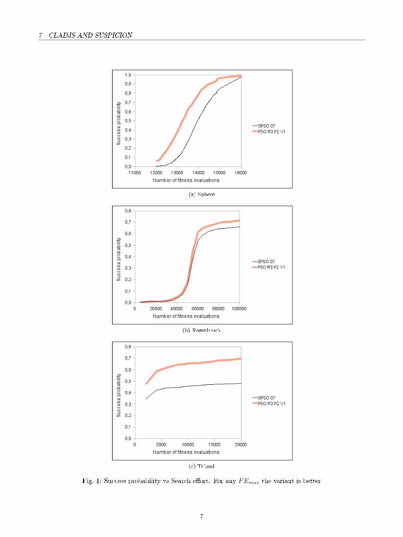
6.3 Highly multimodal problems

Table 8 and �gure 3 are for highly multimodal problems. The good news is that our modi�ed PSO is also bettereven for some highly multimodal problems. It is not true all the time (see Griewank or Cellular phone), but itwas not its aim, anyway.

7 Claims and suspicion

We have seen that it is possible to improve Standard PSO 2007 by modifying the velocity update equationand the initialisation schemes. However, this improvement is not valid across all kinds of problems, and notvalid across all criterions (in particular, it may be depending on the number of �tness evaluations). Also,the improvement is not always very impressive. Thus, this study incites us to be suspicious when readingan assertion like �My PSO variant is far better than Standard PSO�. Such a claim has to be very carefullysupported, by a rigorous de�nition of what �better� means, and by signi�cant results on a good �representative�benchmark, on a large range of maximum number of �tness evaluations. Also, we have to be very careful whenusing the mean best criterion for comparison, for it may be meaningless. And, of course, the proposed PSOvariant should be compared to the current Standard PSO, and not to an old bad version.

6

7 CLAIMS AND SUSPICION

(a) Sphere

(b) Rosenbrock

(c) Tripod

Fig. 1: Success probability vs Search e�ort. For any FEmax the variant is better

7


(a) Schwefel (b) Pressure vessel

(c) Compression spring (d) Gear train

Fig. 2: On the Schwefel and Pressure vessel problems PSO R3 P2 V1 is slightly better than SPSO 07 for anynumber of �tness evaluations. On the Compression spring problem, it is true only when the number of �tnessevaluations is greater than a given value (about 19000). So, on this problem, either claim �SPSO 07 is better�or �PSO R3 P2 V1 is better� is wrong

8


(a) Rastrigin

(b) Griewank

(c) Ackley (d) Cellular phone

Fig. 3: Success probability for some highly multimodal problems. Although designed for moderately multimodalproblems, PSO R3 P2 V1 is even sometimes good for these problems. But not always

9

8 HOME WORK

Tab. 8: Highly multimodal problems. See 9.3 for details

Search Requiredspace accuracy

CEC 2005 Rastrigin [−5, 5]10 0.01

CEC 2005 Griewank [−600, 600]10 0.01(not rotated)

CEC 2005 Ackley [−32, 32]10 0.0001(not rotated)

Cellular phone [0, 100]20 10−8

8 Home work

The speci�c improvement modi�cation of SPSO 07 used here was for moderately multimodal problems, in lowdimension. Let us call them M-problems. Now, what could be an e�ective speci�c modi�cation for another classof problems? Take, for example the class of highly multimodal problems, but still in low dimension (smallerthan 30). Let us call them H-problems.

First, we have to de�ne a small representative benchmark. Hint: include Griewank 10D, from the CEC 2005benchmark (no need to use the rotated function). Second, we have to understand in which way the di�cultyof an H-problem is di�erent from that of an M-problem. Hint: on an H-problem, SPSO 07 is usually less easilytrapped into a local minimum, just because the attraction basins are small. On the contrary, if a particle isinside the �good� attraction basin (the one of the global optimum), it may even leave it prematurely. And third,we have to �nd what options are needed to cope with the found speci�c di�culty(ies). Hint: just make surethe current attraction basin is well exploited, a quick local search may be useful. A simple way is to de�nea local area around the best known position, and to sample its middle (PSO L4)2. With just this option, animprovement seems possible, as we can see from �gure 4 for the Griewank function. However, it does not workvery well for Rastrigin.

All this will probably be the topic of a future paper, but for the moment, you can think at it yourself. Goodluck!

2 Let g = (g1,g2, . . . , gD) be the best known position. On each dimension i, let pi and p′i are the nearest coordinates of

known points, "on the left", and "on the right" of gi. The local area H is the D-rectangle (hyperparallelepid) cartesian product

⊗i

[gi − α (gi − pi) , gi + α

(p′

i − gi

)]with, in practice, α = 1/3. Then its center is sampled. Usually, it is not g.

10

9 APPENDIX

Fig. 4: Griewank, comparison between SPSO 07 and PSO L4. For a highly multimodal problem, a very simplelocal search may improve the performance.

9 Appendix

9.1 Formulae for the benchmark

Tab. 9: Benchmark details

Formula

Sphere −450 +30∑d=1

(xd − od)2 The random o�set vectorO = (o1, · · · , o30)

is de�ned by its C code.This is the solution point.

Rosenbrock 390 +10∑d=2

(100

(z2d−1 − zd

)2+ (zd−1 − 1)2

)The random o�set vector

O = (o1, · · · , o10)with zd = xd − od + 1 is de�ned by its C code.

This is the solution pointThere is also a local minimum on

(o1 − 2, · · · , o30). The �tness value is then394.

Tripod

1−sign(x2)2 (|x1|+ |x2 + 50|)

+ 1+sign(x2)2

1−sign(x1)2 (1 + |x1 + 50|+ |x2 − 50|)

+ 1+sign(x1)2 (2 + |x1 − 50|+ |x2 − 50|)

with

{sign (x) = −1 if x ≤ 0

= 1 else

The solution point is (0,−50)11

9.2 Formulae for the other moderately multimodal problems 9 APPENDIX

O�set for Sphere/Parabola (C source code)

static double o�set_0[30] = { -3.9311900e+001, 5.8899900e+001, -4.6322400e+001, -7.4651500e+001, -1.6799700e+001,-8.0544100e+001, -1.0593500e+001, 2.4969400e+001, 8.9838400e+001, 9.1119000e+000, -1.0744300e+001, -2.7855800e+001, -1.2580600e+001, 7.5930000e+000, 7.4812700e+001, 6.8495900e+001, -5.3429300e+001, 7.8854400e+001,-6.8595700e+001, 6.3743200e+001, 3.1347000e+001, -3.7501600e+001, 3.3892900e+001, -8.8804500e+001, -7.8771900e+001, -6.6494400e+001, 4.4197200e+001, 1.8383600e+001, 2.6521200e+001, 8.4472300e+001 };

O�set for Rosenbrock (C source code)

static double o�set_2[10] = { 8.1023200e+001, -4.8395000e+001, 1.9231600e+001, -2.5231000e+000, 7.0433800e+001,4.7177400e+001, -7.8358000e+000, -8.6669300e+001, 5.7853200e+001};

9.2 Formulae for the other moderately multimodal problems

9.2.1 Schwefel

The function to minimise is

f (x) = −450 +10∑d=1

(d∑k=1

xk − ok

)2

The search space is [−100, 100]10. The solution point is the o�set O = (o1, . . . , o10), where f = −450.

O�set (C source code)

static double o�set_4[30] =

{ 3.5626700e+001, -8.2912300e+001, -1.0642300e+001, -8.3581500e+001, 8.3155200e+001, 4.7048000e+001,-8.9435900e+001, -2.7421900e+001, 7.6144800e+001, -3.9059500e+001};

9.2.2 Pressure vessel

Just in short. For more details, see[9, 10, 11]. There are four variables

x1 ∈ [1.125, 12.5] granularity 0.0625x2 ∈ [0.625, 12.5] granularity 0.0625x3 ∈ ]0, 240]x4 ∈ ]0, 240]

and three constraints

g1 := 0.0193x3 − x1 ≤ 0g2 := 0; 00954x3 − x2 ≤ 0g3 := 750× 1728− πx2

3

(x4 + 4

3x3

)≤ 0


f = 0.06224x1x3x4 + 1.7781x2x23 + x2

1 (3.1611x+ 19.84x3)

The analytical solution is (1.125, 0.625, 58.2901554, 43.6926562)which gives the �tness value 7,197.72893. Totake the constraints into account, a penalty method is used.

12

9 APPENDIX 9.3 Formulae for the highly multimodal problems

9.2.3 Compression spring

For more details, see[9, 10, 11]. There are three variables

x1 ∈ {1, . . . , 70} granularity 1x2 ∈ [0.6, 3]x3 ∈ [0.207, 0.5] granularity 0.001

and �ve constraints

g1 := 8CfFmaxx2

πx33

− S ≤ 0g2 := lf − lmax ≤ 0g3 := σp − σpm ≤ 0g4 := σp − Fp

K ≤ 0g5 := σw − Fmax−Fp

K ≤ 0

with

Cf = 1 + 0.75 x3x2−x3

+ 0.615x3x2

Fmax = 1000S = 189000lf = Fmax

K + 1.05 (x1 + 2)x3

lmax = 14σp = Fp

Kσpm = 6Fp = 300K = 11.5× 106 x4

38x1x3

2

σw = 1.25

and the function to minimise is

f = π2x2x23 (x1 + 1)

4

The best known solution is (7, 1.386599591, 0.292)which gives the �tness value 2.6254214578. To take theconstraints into account, a penalty method is used.

9.2.4 Gear train

For more details, see[9, 11]. The function to minimise is

f (x) =(

16.931

− x1x2

x3x4

)2

The search space is {12, 13, . . . , 60}4. There are several solutions, depending on the required precision. Forexample f (19, 16, 43, 49) = 2.7× 10−12

9.3 Formulae for the highly multimodal problems

9.3.1 Rastrigin


f = −230 +10∑d=1

((xd − od)2 − 10 cos (2π (xd − od))

)The search space is [−5, 5]10. The solution point is the o�set O = (o1, . . . , o10), where f = −330.

13

9.3 Formulae for the highly multimodal problems 9 APPENDIX


static double o�set_3[30] ={ 1.9005000e+000, -1.5644000e+000, -9.7880000e-001, -2.2536000e+000, 2.4990000e+000, -3.2853000e+000,

9.7590000e-001, -3.6661000e+000, 9.8500000e-002, -3.2465000e+000};

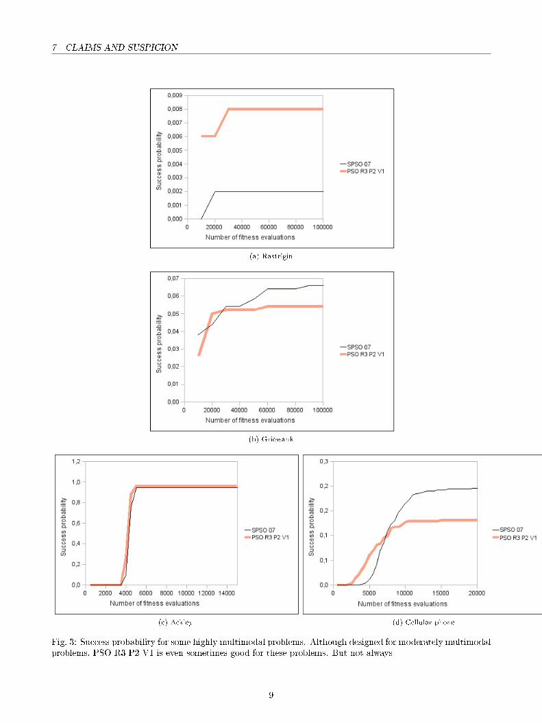
9.3.2 Griewank


f = −179 +∑10d=1 (xd − od)2

4000−

10∏d=1

cos(xd − od√

d

)The search space is [−600, 600]10 .The solution point is the o�set O = (o1, . . . , o10), where f = −180.


static double o�set_5[30] ={ -2.7626840e+002, -1.1911000e+001, -5.7878840e+002, -2.8764860e+002, -8.4385800e+001, -2.2867530e+002,

-4.5815160e+002, -2.0221450e+002, -1.0586420e+002, -9.6489800e+001};

9.3.3 Ackley


f = −120 + e+ 20e−0.2

√1D

∑10

d=1(xd−od)2

− e1D

∑10

d=1cos(2π(xd−od))

The search space is [−32, 32]10 .The solution point is the o�set O = (o1, . . . , o10), where f = −140.


static double o�set_6[30] ={ -1.6823000e+001, 1.4976900e+001, 6.1690000e+000, 9.5566000e+000, 1.9541700e+001, -1.7190000e+001,

-1.8824800e+001, 8.5110000e-001, -1.5116200e+001, 1.0793400e+001};

9.3.4 Cellular phone

This problem arises in a real application, on which I have worked in the telecommunications domain. However,here, all constraints has been removed, except of course the ones given by the search space itself. We havea square �at domain [0, 100]2, in which we want to put M stations. Each station mk has two coordinates(mk,1,mk,2). These are the 2M variables of the problem. We consider each �integer� point of the domain, i.e.(i, j) , i ∈ {0, 1, . . . , 100} , j ∈ {0, 1, . . . , 100}. On each integer point, the �eld induced by the station mk is givenby

fi,j,mk)=1

(i−mk,1)2 + (j −mk,2)

2 + 1

and we want to have at least one �eld that is not too weak. Finally, the function to minimise is

f =1∑100

i=1

∑100j=1 maxk (fi,j,mk

)

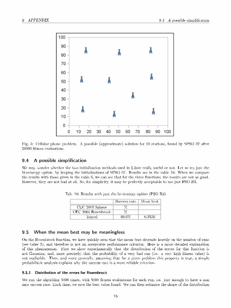
In this paper, we set M = 10 . Therefore the dimension of the problem is 20. The objective value is0.005530517. This is not the true minimum, but enough from an engineering point of view. Of course, inreality we do not know the objective value. We just run the algorithm several times for a given number of�tness evaluations, and keep the best solution. From the �gure 5 we can see a solution found by SPSO 07 after20000 �tness evaluations. Actually, for this simpli�ed problem, more e�cient methods do exist (Delaunay'stessellation, for example), but those can not be used as soon as we introduce a third dimension and moreconstraints, so that the �eld is not spherical any more.

14

9 APPENDIX 9.4 A possible simpli�cation

Fig. 5: Cellular phone problem. A possible (approximate) solution for 10 stations, found by SPSO 07 after20000 �tness evaluations

9.4 A possible simpli�cation

We may wonder whether the two initialisation methods used in 5.2are really useful or not. Let us try just thebi-strategy option, by keeping the initialisations of SPSO 07. Results are in the table 10. When we comparethe results with those given in the table 6, we can see that for the three functions, the results are not as good.However, they are not bad at all. So, for simplicity, it may be perfectly acceptable to use just PSO R3.

Tab. 10: Results with just the bi-strategy option (PSO R3)


CEC 2005 Sphere %CEC 2005 Rosenbrock %

Tripod 60.6% 0.3556

9.5 When the mean best may be meaningless

On the Rosenbrock function, we have quickly seen that the mean best depends heavily on the number of runs(see table 3), and therefore is not an acceptable performance criterion. Here is a more detailed explanationof this phenomenon. First we show experimentally that the distribution of the errors for this function isnot Gaussian, and, more precisely, that the probability of a very bad run (i.e. a very high �tness value) isnot negligible. Then, and more generally, assuming that for a given problem this property is true, a simpleprobabilistic analysis explains why the success rate is a more reliable criterion.

9.5.1 Distribution of the errors for Rosenbrock

We run the algorithm 5000 times, with 5000 �tness evaluations for each run, i.e. just enough to have a nonzero success rate. Each time, we save the best value found. We can then estimate the shape of the distribution

15

9.5 When the mean best may be meaningless 9 APPENDIX

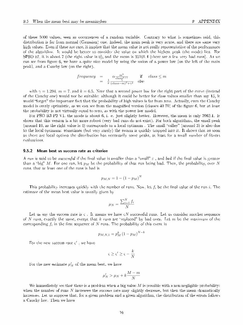
of these 5000 values, seen as occurrences of a random variable. Contrary to what is sometimes said, thisdistribution is far from normal (Gaussian) one. Indeed, the main peak is very acute, and there are some veryhigh values. Even if these are rare, it implies that the mean value is not really representative of the performanceof the algorithm. It would be better to consider the value on which the highest peak (the mode) lies. ForSPSO 07, it is about 7 (the right value is 0), and the mean is 25101.4 (there are a few very bad runs). As wecan see from �gure 6, we have a quite nice model by using the union of a power law (on the left of the mainpeak), and a Cauchy law (on the right).

frequency = α mk

classk+1 if class ≤ m= 1

πγ

(class−m)2+γ2 else

with γ = 1.294, m = 7, and k = 6.5. Note that a second power law for the right part of the curve (insteadof the Cauchy one) would not be suitable: although it could be better for class values smaller than say 15, itwould �forget� the important fact that the probability of high values is far from zero. Actually, even the Cauchymodel is overly optimistic, as we can see from the magni�ed version (classes 40-70) of the �gure 6, but at leastthe probability is not virtually equal to zero, as with the power law model.

For PSO R3 P2 V1, the mode is about 6, i. e. just slightly better. However, the mean is only 3962.1. Itshows that this version is a bit more robust (very bad runs do not exist). For both algorithms, the small peak(around 10, as the right value is 4) corresponds to a local optimum . The small �valley� (around 3) is also dueto the local optimum: sometimes (but very rarely) the swarm is quickly trapped into it. It shows that as soonas there are local optima the distribution has necessarily some peaks, at least for a small number of �tnessevaluations.

9.5.2 Mean best vs success rate as criterion

A run is said to be successful if the �nal value is smaller than a �small� ε , and bad if the �nal value is greaterthan a �big� M . For one run, let pM be the probability of that run being bad. Then, the probability, over Nruns, that at least one of the runs is bad is

pM,N = 1− (1− pM )N

This probability increases quickly with the number of runs. Now, let fi be the �nal value of the run i. Theestimate of the mean best value is usually given by

µN =∑Ni=1 fiN

Let us say the success rate is ς . It means we have ςN successful runs. Let us consider another sequenceof N runs, exactly the same, except that k runs are �replaced� by bad ones. Let m be the maximum of thecorresponding fi in the �rst sequence of N runs. The probability of this event is

pM,N,1 = pkM (1− pM )N−k

For the new success rate ς ′ , we have

ς ≥ ς ′ ≥ ς − k

N

For the new estimate µ′N of the mean best, we have

µ′N > µN + kM −mN

We immediately see that there is a problem when a big valueM is possible with a non negligible probability:when the number of runs N increases the success rate may slightly decrease, but then the mean dramaticallyincreases. Let us suppose that, for a given problem and a given algorithm, the distribution of the errors followsa Cauchy law. Then we have

16

9 APPENDIX 9.5 When the mean best may be meaningless

(a) Global shape

(b) Zoom" on classes 40 to 70

Fig. 6: Rosenbrock. Distribution of the best value over 5000 runs. On the �zoom�, we can see that the Cauchymodel, although optimistic, gives a better idea of the distribution than the power law model for class valuesgreater than 40

17

References References

pM = 0.5− 1π

arctan(M

γ

)With the parameters of the model of the �gure 6, we have for example p5000 = 8.3 × 10−5. Over N = 30

runs, the probability to have at least one bad run (�tness value greater than M = 5000) is low, just 2.5× 10−3.Let us say we �nd an estimate of the mean to be m. Over N = 1000 runs, the probability is 0.08, which is quitehigh. It may easily happen. In such a case, even if for all the other runs the best value is about m, the newestimate is about (4999m+ 5000) /1000, which may be very di�erent from m. In passing, and if we look at thetable 3, this simpli�ed explanation shows that for Rosenbrock a Cauchy law based model is indeed optimistic.

In other words, if the number of runs is too small, you may never have a bad one, and therefore, wronglyestimate the mean best, even when it exists. Note that in certain cases the mean may not even exist at all(for example, in case of a Cauchy law), and therefore any estimate of a mean best is wrong. That is whyit is important to estimate the mean for di�erent N values (but of course with the same number of �tnessevaluations). If it seems not stable, forget this criterion, and just consider the success rate, or, as seen above,the mode. As there are a lot of papers in which the probable existence of the mean is not checked, it is worthinsisting on it: if there is no mean, giving an �estimate� of it is not technically correct. Worse, comparing twoalgorithms based on such an �estimate� is simply wrong.

References

[1] PSC, �Particle Swarm Central, http://www.particleswarm.info.�

[2] CEC, �Congress on Evolutionary Computation Benchmarks,http://www3.ntu.edu.sg/home/epnsugan/,�2005.

[3] L. Gacôgne, �Steady state evolutionary algorithm with an operator family,� in EISCI, (Kosice, Slovaquie),pp. 373�379, 2002.

[4] M. Clerc, �Math Stu� about PSO, http://clerc.maurice.free.fr/pso/.�

[5] G. Marsaglia and A. Zaman, �The kiss generator,� tech. rep., Dept. of Statistics, U. of Florida, 1993.

[6] T.-T. Wong, W.-S. Luk, and P.-A. Heng, �Sampling with Hammersley and Halton points,� Journal of

Graphics Tools, vol. 2 (2), pp. 9�24, 1997.

[7] M. Clerc, �The mythical balance, or when PSO doe not exploit,� Tech. Rep. MC2008-10-31, 2008.

[8] I. Zelinka, �SOMA - Self-Organizing Migrating Algorithm,� in New Optimization Techniques in Engineering,pp. 168�217, Heidelberg, Germany: Springer, 2004.

[9] E. Sandgren, �Non linear integer and discrete programming in mechanical design optimization,� 1990. ISSN0305-2154.

[10] M. Clerc, Particle Swarm Optimization. ISTE (International Scienti�c and Technical Encyclopedia), 2006.

[11] G. C. Onwubolu and B. V. Babu, New Optimization Techniques in Engineering. Berlin, Germany: Springer,2004.

18

Documents

A method to improve Standard PSO