A method to recover water-wave profiles from pressure measurements

Vishal Vasana,∗, Katie Oliverasb, Diane Hendersona, Bernard Deconinckc

aDepartment of Mathematics, Pennsylvania State University, University Park, PA 16802bDepartment of Mathematics, Seattle University, Seattle, WA 98122

cDepartment of Applied Mathematics, University of Washington, Seattle, WA 98195

Abstract

An operational formulation is proposed for reconstructing a time series of water surface displacement

from waves using measurements from a pressure transducer located at an arbitrary depth. The

approach is based on the fully nonlinear formulation for pressure below traveling-wave solutions

of Euler’s equations developed in [1]. Its validity is tested using experiments in which both the

pressure and the surface displacement are measured. The experiments include a wave system that

is Galilean invariant – cnoidal waves, and wave systems that are not – reflected cnoidal waves and

wave groups. We find that since the proposed formulation is nonlinear, it reproduces the amplitude

spectrum of the measured surface displacements better than the hydrostatic model and better than

the linear model that takes into account the pressure response factor due to small amplitude waves

(the transfer function). Both the proposed formula and the transfer function reconstruct the surface

reasonably well, with the proposed formula being about 5% more accurate.

Keywords: water waves, pressure, recovery, measurement

1. Introduction

Pressure transducers are a common device for measuring surface water waves in both the lab-

oratory and the field. However, the inversion from time series of pressure to time series of surface

displacement is nontrivial. The relationship between pressure and surface displacement, based

on the Stokes boundary value problem [2], is nonlinear and involves water particle velocities. In

∗Corresponding author at: Department of Mathematics, Pennsylvania State University, University Park, PA16802

Email address: vxv10@psu.edu (Vishal Vasan)

Preprint submitted to Elsevier April 28, 2015

practice, various approximate relationships are used. A common [3] relation between the surface

displacement spectrum Sf and the pressure spectrum Sp is

Sf = NSp/Kp, (1)

where N is an empirical factor, and

Kp =cosh k(h+ z)

cosh kh(2)

is the pressure response factor, which is obtained from linear theory and takes into account pressure

due to wave motion. Here, h is the water depth; k is the radian wavenumber related to radian wave

frequency ω through the linear dispersion relation ω2 = gk tanh(kh); g is the acceleration of gravity

and z < 0 is the vertical depth of the pressure transducer, measured positive upward from the

still water level. The empirical factor N = 1 corresponds to linear wave theory. The conventional

wisdom from the Shore Protection Manual [3] is that N decreases with decreasing period; N > 1

for long-period waves, and N < 1 for short-period waves.

There have been many field and laboratory studies to determine if linear theory provides an

adequate relationship between pressure measurements and surface displacement, and some disagree-

ment exists. Bishop & Donelan [4] reviewed these studies. They concluded that linear wave theory

is adequate for obtaining surface wave heights from pressure gage data to within 5%, except when

measuring waves in shallow water. For waves in shallow water, they concurred with [5] that one

must use N 6= 1 in order to account for currents and wave nonlinearity. Also energy from higher

frequency waves is not recovered adequately by (1) because the higher frequency velocities fall

off rapidly with increasing depth, because of inherent limitations of the pressure transducers and

because of spectral leakage to high frequencies due to the form of Kp.

Typically, nonlinear effects are included using a Stokes expansion to obtain higher order cor-

rections. There have been studies using Stokes expansions to 2nd order [5], to 3rd order, and 5th

order [6]. Tsai et. al [7] reviewed these results, some of which showed improvement over linear

theory and some of which did not. They concluded both that “These seemingly incoherent results

in fact only reflect the different wave conditions being studied.” and that “... it is universally

understood that the non linear correction is essential in shallow water or in surf zone.” Alternative

approaches have been considered. For example, Chen [8] used a higher order expansion to find an

2

empirical nonlinear transfer function with a frequency parameter and a depth of gage submergence

parameter. Kuo & Chiu [9] used dimensional analysis to develop an empirical formula from data,

which Baquerizo & Losada [10] showed could be obtained from the pressure response factor (with

a reply in [11]). Fully nonlinear models for surface displacement recovery based on the equations

for traveling water waves were presented in [1, 12–15]. A neural network approach is given in [16]

and [17].

The subject remains an area of importance and on-going work. Indeed, the array of about 40

DART (Deep-ocean Assessment and Reporting of Tsunamis) buoys used for obtaining real-time

surface-displacement data for tsunami forecasting rely on pressure measurements, as do measure-

ments of storm surge from hurricanes [18].

In this paper, we address the need for obtaining a nonlinear mapping from pressure to surface

displacement following Oliveras et al [1]. Rather than starting with the Stokes boundary value

problem and proceeding with a perturbation expansion in the surface displacement and velocity

potential, we started with a reformulation of the Stokes boundary value problem given by [19].

From this representation, we found an exact formulation for the surface displacement that requires

the numerical solution of a nonlocal, nonlinear equation. The errors with respect to nonlinearity do

not exceed machine precision. In this formulation, we make two assumptions: (i) that the pressure

transducers are situated at the bottom of the fluid domain, and (ii) that surface displacements are

due to a traveling wave system. This theory is reviewed in §2. Many of the papers discussed above,

such as [8] have shown that transducer depth is important. Therefore in §3 we expand the result in

[1] to allow for an arbitrary depth of the pressure transducer. Currents are important as well. Thus

in Appendix A we discuss an extension to the theory that allows for a constant vorticity following

Vasan & Oliveras [20]. A summary of the theoretical results presented is:

• The general formula from [1] has no approximation on type of nonlinearity; however solutions

must be found numerically, albeit to machine precision.

• To obtain an explicit, operational formulation, we truncate the order of nonlinearity and

propose a formula to replace (1) in practice. (The fully nonlinear formulation from [1] makes

asymptotics quite straightforward.)

• The proposed formulation assumes a traveling wave system, and so requires a wave speed,

which is assumed to be the same for all frequency components.

3

– The standard, linear inversion, (1) with the empirical constant N = 1, is a special case

of the formulation presented here, thus, the assumption of traveling waves does not limit

the associated generality of the present results more than (1) does.

– Since measurements comprise time series at fixed locations, some value of the wave speed

is required by all models to map from time data to spatial data.

– Oliveras & Vasan [21] reformulated the mapping so that the value of the speed is not

required. We do not use their results herein, as discussed in §3.

• The formulation presented here allows the pressure transducer to be at any depth in the water

column.

• The new formulation allows for constant vorticity, which introduces new phenomena.

In [1] we developed various approximations to their fully nonlinear pressure-to-surface displace-

ment mapping. We compared the fully nonlinear mapping and these approximations with numerical

solutions and with experimental measurements of solitary waves that used both surface capacitance

gages and bottom, pressure transducers. Here we report also on experimental comparisons with

predictions to see if the proposed formula works for wave systems that break the assumption of a

traveling wave system. The experimental apparatus is presented in §4. Results are presented in §5for experiments that use cnoidal waves, which give a periodic, traveling wave system as assumed

by the theory, and for experiments that use reflecting cnoidal waves and wave groups, neither of

which comprise traveling wave systems. We summarize results in §6.

Our main conclusion is that since the proposed formula is nonlinear, it reproduces the amplitude

spectrum of the measured surface displacements better than does the transfer function (1) with the

empirical constant N = 1. The experiments show that both the proposed formula and the transfer

function reconstruct the surface displacement reasonably well, with predictions from the proposed

formula being about 5% more accurate. Hence, we claim that the proposed formula presented

here provides a better mapping from time series measurements of pressure to time series of surface

displacement than is otherwise available. It is more accurate than (1), requires just one more Fourier

transform, is no less general because of the assumption of traveling waves, and it can include an

arbitrary depth for the pressure transducer.

4

x

z

z = η(x, t)

D

z = −h

z = 0

P (x,−h, t)

Figure 1: The fluid domain D for the water wave problem. A pressure sensor is indicated at the

bottom. In our calculations the pressure measurement is assumed to be a point measurement.

2. Theory

Consider Euler’s equations describing the dynamics of the surface of an ideal irrotational fluid

in two dimensions (with a one-dimensional surface):

φxx + φzz = 0, (x, z) ∈ D, (3)

φz = 0, z = −h, (4)

ηt + ηxφx = φz, z = η(x, t), (5)

φt +1

2

(φ2x + φ2z

)+ gη = 0, z = η(x, t), (6)

where φ(x, z, t) represents the velocity potential of the fluid with surface elevation η(x, t). A solution

to the above set of equations consists of finding a potential φ that satisfies Laplace’s equation inside

the fluid domain D, sketched in Figure 1, as well as finding the graph of the free surface η. Below

we pose the problem on the whole line x ∈ R, assuming the velocities (and surface profile) decay at

infinity. The problem may also be posed using periodic boundary conditions. The only change in

the resulting relations being that the Fourier series is employed in the place of the Fourier transform.

Our goal is to relate the pressure measured at a sensor P (x0,−h, t), which is also sketched in

Figure 1, located on the bottom boundary of the fluid, to the surface elevation profile η(x0, t).

As stated, equations (3-6) do not involve the pressure field. However, we note that the following

Bernoulli condition valid in the interior of the fluid:

φt +1

2

(φ2x + φ2z

)+ gz +

P (x, z, t)

ρ= 0, − h ≤ z ≤ η(x, t). (7)

5

The overall scheme is as follows. Since (7) is valid at the bottom boundary, we employ this relation

to convert the pressure measurement into a condition on the velocity potential at z = −h. In

addition, we note from equations (5-6), that the velocity potential at the surface is related to the

surface elevation profile. Since the potential φ satisfies Laplace’s equation, the boundary values of

the potential at z = −h and z = η must be related. This consistency of boundary values forms the

basis of our reconstruction method.

The scheme described in the previous paragraph involves connecting boundary data at the

bottom and top surfaces. Setting φz(x,−h, t) = 0 in equation (7) we obtain a relation between

the bottom pressure P (x,−h, t) and φ(x,−h, t). A major difficulty in the problem of surface

reconstruction, however, is that the input data is typically a time series of the pressure at z = −hfor a single spatial point (or discrete set of points), i.e., Pj(xj ,−h, t), j = 1, 2, . . ., where xj need

not be spaced close together. In our experiments, as well as in field experiments, we typically

deal with only one spatial location x0. Therefore, we require a method to convert P (x0,−h, t) to

P (x,−h, t). Further, having recovered P (x,−h, t), we seek φ(x,−h, t) through (7). We claim this

is not practical without further simplification. To see why, consider (7) as a partial differential

equation for φ(x,−h, t) with P (x,−h, t) as a forcing term. Evidently we require knowledge of an

initial state for φ(x,−h, t), i.e., an initial condition.

In the following, we restrict to the case of a traveling wave moving with velocity c. This

assumption permits us to translate time series data to spatial information, establishes the initial

state of the fluid (indeed the state for all time) and permits the study of nonlinear effects. One of

the primary aims of the current work is to understand how nonlinear effects may be incorporated

to increase the accuracy of surface reconstruction. Of course, assuming a traveling wave comes at a

cost. The speed of the wave is required to translate the time series data to a spatial measurement.

A pictographic overview of the reconstruction method is shown in Figure 2. Although not

explictly indicated in the figure, the wave speed does appear in the reconstruction of η(x, t0) from

P (x,−h, t0), i.e., the central part of Figure 2. In [22] the authors investigated the dependence on

the speed c for this part of the reconstruction algorithm for numerically computed traveling water

wave solutions to Euler’s equations. They found that the method introduced in [1] was particularly

insensitive to errors in the wave speed. In the present work we investigate the effect of the speed of

the wave particularly for the conversion from time series to spatial data for pressure measurements

from physical experiments. For the conversion from P (x,−h, t0)→ η(x, t0), in the current work, we

6

Consistentboundary

conditions of the Laplace equation

Wave speed

Bernoulli equation (11)

Wave speed

Bernoulli equation (9)

Figure 2: Summary of the surface reconstruction algorithm.

employ three speed-independent asymptotic reductions obtained from the fully nonlinear method

of [1]. They are the hydrostatic model, the transfer function (1) with the empirical constant N = 1,

and the proposed formula (23).

Remark 1. In §5 we present the reconstruction of the water wave surface for two interacting

traveling waves and a wave group. These experiments imply different choices for the wave speed to

convert the time series data into a spatial measurement. This is, in part, why we do not use the

traveling wave variable x− ct in Figure 2.

Now we present a review of the derivation for the fully nonlinear reconstruction algorithm from

P (x,−h, t0) → η(x, t0) under the assumption of a traveling wave [1]. Our goal is to obtain from

this the asymptotic reconstruction formulae. We introduce ξ = x − ct and assume all dynamical

quantities depend only on ξ, so that x and t-derivatives become ξ-derivatives, the latter multiplied

by −c. The Bernoulli and kinematic boundary conditions at the free surface z = η become:

−cηξ + ηξΦξ = Φz, z = η(ξ), (8)

−cΦξ +1

2

(Φ2ξ + Φ2

z

)+ gη = 0, z = η(ξ), (9)

where Φ(ξ, z) = φ(x, z, t). Equations (8-9) are an algebraic set of relations for the velocities at the

surface from which we obtain

Φξ(ξ, η) = c−√c2 − 2gη

1 + η2ξ, (10a)

Φz(ξ, η) = −ηξ√c2 − 2gη

1 + η2ξ, (10b)

7

where for c > 0 we choose the − sign, to ensure that the local horizontal velocity is less than the

wave speed [23]. Similarly, for c < 0 the + sign should be chosen. In the following we choose c > 0,

restricting to rightward traveling waves. This simple calculation allows us to express the gradient

of the velocity potential at the surface directly in terms of the surface elevation.

A similar consideration for the Bernoulli condition (7) at the bottom boundary z = −h leads to

− cQξ +1

2Q2ξ − gh+

P (ξ,−h)

ρ= 0, (11)

where Q(ξ) = Φ(ξ,−h) is the velocity potential at the bottom of the fluid, and we have changed to

the traveling coordinate frame as before. Then (11) is a quadratic equation for Qξ from which we

find

Qξ = c−√c2 − 2p, (12)

where p(ξ) is the non-static part of the pressure at the bottom in the traveling coordinate frame,

scaled by the fluid density: p(ξ) = −gh + P (ξ,−h)/ρ. As before we choose the − sign to be

consistent with rightward traveling waves.

Within the bulk of the fluid D,

Φξξ + Φzz = 0, (13)

where the boundary conditions given in (10a, 10b) and (12) must also be satisfied. A potential

consistent with irrotational gravity waves must satisfy the associated kinematic conditions (4) and

(5). Thus we let

Φ(ξ, z) =1

2π

∫ ∞−∞

eikξΨ(k) cosh (k (z + h)) dk, (14)

so that equation (4) is automatically satisfied. Here, we have assumed that the fluid velocities decay

at infinity in the horizontal direction. Using the boundary condition at the bottom for Φξ we find

1

2π

∫ ∞−∞

ikeikξΨ(k) dk = c−√c2 − 2p, (15)

so that

ikΨ(k) = 2πcδ(k)−F{√

c2 − 2p}

(k), (16)

where δ(k) is the Dirac delta function and F denotes the Fourier transform: F{y(ξ)}(k) =

8

∫∞−∞ y(ξ) exp(−ikξ)dξ. The form (14) implies Φξ(ξ, z) at the surface z = η, which is given by

Φξ(ξ, η) =1

2π

∫ ∞−∞

eikξikΨ(k) cosh (k (η + h)) dk (17)

= c− 1

2π

∫ ∞−∞

eikξ cosh (k (η + h))F{√

c2 − 2p}

(k) dk. (18)

Using (18) and the boundary condition (10a), the consistency of boundary conditions leads to the

nonlocal, fully nonlinear relationship

√c2 − 2gη

1 + η2ξ=

1

2π

∫ ∞−∞

eikξ cosh (k (η + h))F{√

c2 − 2p}

(k) dk. (19)

The above relation is a nonlinear equation for η given p and c. A rigorous justification of the above

relation is presented in [1]. The analogous relationship for periodic boundary conditions is given

by replacing integrals with the appropriate summation.

One advantage of a fully nonlinear model such as (19), is the ease with which various approximate

models, valid in different physical regimes, may be derived. Let ε, µ represent the amplitude and

shallowness parameters, i.e., ε = a/h and µ = h/L, where a is the wave amplitude and L is the

characteristic horizontal length scale (say, the wavelength). We define the following non-dimensional

variables

ξ̃ = ξ/L, z̃ = z/h, η̃ = η/a, k̃ = Lk, c̃ = c/√gh, p̃ = p/ga.

Equation (19) in non-dimensional variables is given by√c̃2 − 2εη̃

1 + ε2µ2η̃2ξ̃

=1

2π

∫ ∞−∞

eik̃ξ̃ cosh(µk̃ (εη̃ + 1)

)F{√

c̃2 − 2εp̃}

(k̃) dk̃. (20)

One may Taylor expand in ε and/or µ to any required order and obtain asymptotically-equivalent

reduced reconstruction models. In [1], we obtain and compare several models with numerical results

and laboratory experiments on solitons. Here, we quote three of these models in their dimensional

forms and compare their reconstuctions of measured time series of pressure in §5. Two of these are

standard models discussed in §1: the hydrostatic approximation

η =p

g, (21)

and the transfer function (1) with the empirical constant N = 1, which gives a linear, dynamic

correction to the hydrostatic approximation;

F [η] = cosh(kh)F[p

g

]. (22)

9

The third is the proposed model

η =F−1

[cosh(kh)F

[pg

]]1−F−1

[k sinh(kh)F

[pg

]] , (23)

which yields the best results of all of the reduced models in the comparisons reported in [1]. We

call (23) the “heuristic model”. Aside from being common reconstruction methods employed in

practice (in the case of the hydrostatic and transfer function), our study of surface displacement

recovery is limited to these models as none of them have an explicit dependence on the wave-speed

c.

Each of the above models for surface reconstruction can be obtained through an asymptotic

expansion of (19). The hydrostatic model (21) is obtained to lowest order in the shallow water

regime (retaining only O(1) terms or in other words setting ε = µ = 0), whereas the transfer

function (22) is obtained by linearizing the fluid equations, i.e., by expanding (20) in ε and retaining

all terms up to O(ε). The heuristic model (23) can be thought of as a nonlinear correction to the

transfer function. Indeed this model is obtained by including particular terms of a small amplitude

expansion of (19); see [1] for details. We note that each of the above asymptotic models are

independent of the wave speed c. However, higher order models, in µ or ε, typically involve the

wave speed.

We note that the traditional approach to obtaining the transfer function is by linearizing the

equations for surface gravity waves. However, here we obtain the same result by linearizing (19)

which is a consequence of assuming a traveling water wave. Thus, (22) can be formally interpreted

for either traveling waves or small-amplitude linear waves. Consequently, we employ this model

to reconstruct small-amplitude surface gravity waves with no specific speed. Similarly we may

reinterpret (23) in the context of small-amplitude time-dependent wave motion. Indeed, the above

analysis suggests suitable nonlinear corrections to (22) which we claim are relevant to generic time-

dependent shallow water-wave surface profile reconstruction based on our experiments.

In practice, the difference between assuming a traveling wave with speed c and small-amplitude

water waves amounts to choosing a wave speed to convert the time series data P (x0,−h, t) to the

spatial measurement P (x,−h, t0). Mathematically this implies a relationship between the wave

number k and the frequency ω, i.e., ω = ck for nonlinear traveling waves and

ω =√gk tanh(kh), (24)

10

for small amplitude waves. Here we have chosen only one branch of the dispersion relation since, to

be consistent with the fully nonlinear model, we restrict ourselves to waves traveling in one direction

alone. Note that each of the above relations may be solved for k as a function of ω. Consequently,

we observe that the reconstruction models (22) and (23) depend implicitly on the wave speed. See

Section 4.1 for details on the inversion of the dispersion relation (24).

3. Pressure transducer at arbitrary depth

In the following we extend the algorithm of [1] to allow reconstruction of the surface profile

from pressure measurements at an arbitrary height below the free surface. For an extension of the

algorithm that accounts for a constant shear, i.e., constant vorticity, see Appendix A. In either case

we assume a traveling water wave with speed c.

In §2 we assumed the pressure was measured at the bottom boundary. This requirement is not

essential. Here we adapt the method for surface profile reconstruction to the case when the pressure

data is recorded at some height between the free surface and bottom boundary. We restrict ourselves

to a case where the measuring station does not have a significant impact on the fluid flow, so that

the pressure signal P0 is at a constant height z = −z0 (−h < −z0 < min η). Since the potential

Φ(ξ, z) satisfies Laplace’s equation in the domain −h < z < −z0, we employ a similar technique of

consistent boundary conditions to map the given non-static pressure data, p0 = P (ξ,−z0)/ρ− gz0,

to the corresponding pressure signal at the bottom boundary p(ξ,−h) and thus the results from

the previous section become available.

Consider a harmonic function

Φξξ + Φzz = 0, −h < z < −z0,

such that Φz(ξ,−h) = 0 and Φξ(ξ,−z0) is prescribed. Assuming the gradient of Φ decays for large

|ξ| (alternatively, the gradient is periodic in ξ), this boundary-value problem has a well-defined

solution. In particular we obtain the following relation between the Fourier transforms, using (14),

of the components of ∇Φ evaluated at z = −z0:

F [Φz(ξ,−z0)] = −i tanh(k(h− z0))F [Φξ(ξ,−z0)] = 0. (25)

However, ∇Φ is assumed to correspond to the velocity of an inviscid irrotational traveling water

11

wave with speed c. Hence

−cΦξ +1

2Φ2ξ +

1

2Φ2z + p0 = 0, z = −z0, (26)

as a consequence of the Bernoulli condition in the bulk of the fluid. Solving (26) for Φξ and

substituting in (25), we have

F [Φz(ξ,−z0)] = −i tanh(k(h− z0))F[c−

√c2 − 2p0 − [Φz(ξ,−z0)]2

]. (27)

Thus, given a pressure signal at some height −z0, we solve (27) for the vertical velocity at z = −z0.

In numerical tests, a simple iterative scheme based on (27) was sufficient to converge to the true

value. Once Φz(ξ,−z0) is computed we consider the boundary-value problem

Φξξ + Φzz = 0, −h <z < −z0, (28a)

Φz = 0, z = −h, (28b)

Φz = f(ξ), z = −z0, (28c)

where f(ξ) is the solution of (27) for a given p0. The horizontal boundary conditions are assumed

to be either periodic or vanishing at infinity. The solution to (28a-28c) leads to an expression for

Φξ(ξ,−h). Again we assume the potential is consistent with a traveling water wave, so the velocity

component Φξ(ξ,−h) obtained must satisfy the Bernoulli condition at z = −h, (11). Hence, we

obtain the following relation

F[c−

√c2 − 2p

]= sech(k(h− z0))F

[c−

√c2 − 2p0 − [Φz(ξ,−z0)]2

], (29)

where p is the non-static component of the pressure at the bottom boundary z = −h, and we

have used (12) to replace Φξ(ξ,−h). Equations (27) and (29) form the basis for surface elevation

reconstruction from pressure measurements taken in the bulk of the fluid. Once the bottom pressure

p is obtained from these equations we may use (19), or indeed (21-23), to obtain the free surface

profile.

Remark 2. In order to obtain the pressure p(ξ) at z = −h from (27) and (29), we assume the wave-

speed c is known. However, as in the derivation of the reduced models (21-23), in an asymptotic

sense, we can recover p(ξ) from p0(ξ) without the wave-speed. Indeed, in the appropriate scaling,

we observe from (27) that Φz(ξ,−z0) is of the same order as p0(ξ). Hence, from (29) we see that

12

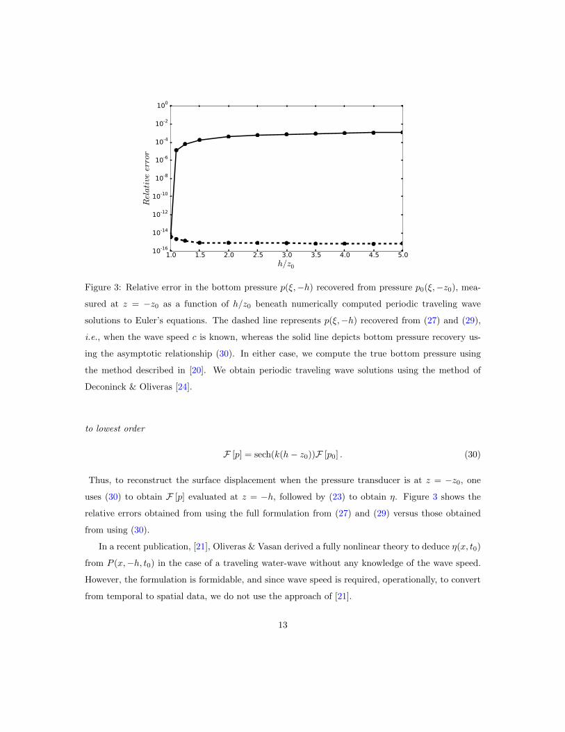
1.0 1.5 2.0 2.5 3.0 3.5 4.0 4.5 5.0h/z0

10-16

10-14

10-12

10-10

10-8

10-6

10-4

10-2

100

Relative

error

Figure 3: Relative error in the bottom pressure p(ξ,−h) recovered from pressure p0(ξ,−z0), mea-

sured at z = −z0 as a function of h/z0 beneath numerically computed periodic traveling wave

solutions to Euler’s equations. The dashed line represents p(ξ,−h) recovered from (27) and (29),

i.e., when the wave speed c is known, whereas the solid line depicts bottom pressure recovery us-

ing the asymptotic relationship (30). In either case, we compute the true bottom pressure using

the method described in [20]. We obtain periodic traveling wave solutions using the method of

Deconinck & Oliveras [24].

to lowest order

F [p] = sech(k(h− z0))F [p0] . (30)

Thus, to reconstruct the surface displacement when the pressure transducer is at z = −z0, one

uses (30) to obtain F [p] evaluated at z = −h, followed by (23) to obtain η. Figure 3 shows the

relative errors obtained from using the full formulation from (27) and (29) versus those obtained

from using (30).

In a recent publication, [21], Oliveras & Vasan derived a fully nonlinear theory to deduce η(x, t0)

from P (x,−h, t0) in the case of a traveling water-wave without any knowledge of the wave speed.

However, the formulation is formidable, and since wave speed is required, operationally, to convert

from temporal to spatial data, we do not use the approach of [21].

13

4. Experimental Apparatus and Procedure

Experiments were conducted in the William G. Pritchard Fluid Mechanics Laboratory in the

Department of Mathematics at Pennsylvania State University to create and measure a variety of

waves for comparisons of surface reconstructions using the three models (21-23). In these experi-

ments the pressure at the bottom of the fluid and the displacement of the air–water interface were

measured simultaneously during wave propagation.

4.1. Apparatus

The wave tank is 50 ft long and 10 inches wide with tempered glass walls and bottom. It was

cleaned with alcohol and filled with tap water to a depth greater than the desired depth, h, so that

the surface could be cleaned. We cleaned the surface using a fan attached to one side of the tank.

It blew a wind that created a surface current that carried contaminants attached to the surface

along the length of the tank to the other end (50ft away). There we used a wet vac to vacuum the

contaminants along with the top few millimeters of fluid. We used a Lory Type C point gage to

measure the resulting water depth h.

We used two types of wave gages: a capacitance gage for measuring surface displacements

directly and a pressure transducer mounted into a hole in the bottom glass panel. The pressure

transducer was a SENZORS PL6T submersible level transducer with a range of 0-4 in. It provided a

0-5V dc output, which was digitized with an NI PCI-6229 analog-to-digital converter using LabView

software. We calibrated this transducer by raising and lowering the water level in the channel.

The pressure measurements had a high-frequency noise component, and thus low-pass filters were

employed.

We implemented two possible low-pass filters. In the first case, by averaging the Fourier am-

plitudes of the high-frequency wave numbers we estimated a noise level. All modes with Fourier

amplitudes less than or equal to this noise level were set to zero. The noise level was chosen so that

the transform cosh(kh) resulted in a smooth reconstruction. Effectively, this filter picked out the

dominant modes. In the second case, the pressure measurements were filtered assuming a suitable

cut-off frequency. For instance, data from a measurement of a 1 Hz cnoidal wave was filtered with

a cut-off frequency of 10 Hz. This smoothing however does not necessarily regularize the hyper-

bolic transforms employed in the transfer and heuristic function approach. To do so we replaced

the original hyperbolic terms with cosh(αkh) and sinh(αkh), where α = 1 if kh < 1 and α = 0

14

otherwise. Thus when α = 0, both transfer and heuristic functions are equivalent to the identity

map. In essence, we wish to apply the recovery algorithm only to the shallow water component of

the measured signal.

Both low-pass filters produced qualitatively similar results in real space. Further, the frequency

corresponding to kh = 1 was close to the largest dominant mode picked out by the first method. In

the experiments discussed below this was around 2 Hz. The heuristic function, being a nonlinear

map from pressure to surface elevation, introduces higher wave number modes into the reconstruc-

tion unlike the transfer function approach. The first method of filtering typically retains a small

number of dominant modes and so is ideally suited to understanding the nonlinear interactions

generated by the heuristic function. However, in practice, we prefer the second method of filtering

the pressure measurements since it is physically motivated and relatively simple to implement.

The capacitance-type surface wave gage consisted of a conducting wire coated with the commer-

cially available superhydrophic coating “Rustoleum’s NeverWet”.The coated wire was connected to

two quartz crystals. One had a fixed oscillation frequency and one had a frequency dependent on

the water height on the coated wire. The difference frequency was read by a Field Programmable

Gate Array (FPGA), NI PCI-7833R. The surface capacitance gage was held in a rack on wheels

that was attached to a programmable belt. We calibrated the capacitance gage by traversing the

rack at a known speed over a precisely machined, trapezoidally-shaped “speed bump”. Time series

of surface displacement were obtained using LabView software that controlled the FPGA board.

The output from the pressure and surface gauges consisted of a time series of the pressure and

surface displacement at a fixed location respectively. Since the theory for surface reconstruction

is based on knowledge of the pressure field, i.e., a spatial measurement, we used the speed of the

wave to translate the time series into a spatial measurement. The choice of speed depends on

the particular type of wave. Thus for a small amplitude wave that is well approximated by the

linearized water-wave equations we chose the phase speed given by the dispersion relation, whereas

for more nonlinear waves we used the programmed wave speed. An alternate choice is the shallow

water wave speed of√gh, where h is the mean depth of the water. We note that all models

considered herein require knowledge of wave speed, since all models make a spatial reconstruction

out of temporal measurements. The conversion from a temporal measurement to a spatial one

involves an assumption on the partial differential equation satisifed by the measured quantity (here

15

the bottom pressure). In the current work we assume the pressure satisfies an equation of the form

pt + ω(−i∂x)p = 0,

where ω(k) is the dispersion relation. Here we choose either ω = ck or the expression given by

(24). The solution to the above differential equation (assuming periodic boundary conditions) can

be written as

p(x, t) =∑n∈Z

einπx/L+iω(n)tF [p0](n),

where p0 is an initial condition and L is the spatial period of the wave. The conversion from a

temporal measurement to a spatial one is equivalent to re-parametrizing the summation above in

terms of ω, rather than k. This involves inverting the dispersion relation. Consequently we see the

need for a one-to-one relation between ω and k, and we limit the discussion to waves traveling in one

direction. Finally we note that the process of temporal to spatial measurment conversion is a type

of smoothing in the case of traveling water waves where k = ω/c. Thus choosing a wave speed c,

in combination with the kh = 1 cutoff, works to bias the reconstruction towards the low frequency

modes. Indeed, both transfer and heuristic functions approximate the hydrostatic reconstruction

for larger values of c.

The waves were generated with a piston-type paddle made from Teflon and machined to fit

the channel with a thin lip around its periphery that served as a wiper with the channel’s glass

perimeter. This wiper minimized leakage around the paddle during paddle motion. The paddle

was attached to a Parker 406 LXR linear motor, controlled using the Aries Controller Program

(ACR) 6 software. The motion of this paddle could be precisely programmed to provide a smooth

stroke profile with a resolution of 1/42000 inch. The theory for programming the paddle motion is

discussed in the next section.

4.2. Theory for wave generation

In order to perform controlled and repeatable experiments, we generated specific known surface

profiles. Hence, here we describe a method to translate a given target surface profile ζ(x, t) into a

corresponding motion of the paddle L(t). Assuming the fluid motion is governed by the equations for

16

inviscid irrotational flow, the velocity potential satisfies the following free-boundary value problem:

φxx + φzz = 0, (x, z) ∈ D, (31)

φt +1

2

(φ2x + φ2z

)+ gη = 0, z = η(x, t), x > L(t), (32)

ηt + ηxφx = φz, z = η(x, t), x > L(t), (33)

φx = L′(t), x = L(t),−h < z < η, , (34)

φz = 0, z = −h, (35)

φx, φz, η → 0 as x→∞, (36)

where L(t) is the position of the paddle, η is the surface displacement and for convenience we

have assumed a semi-infinite wave tank. The fluid domain is given by D = {(x, z) : L(t) < x <

∞,−h < z < η}. The wavemaker problem consists of the following inverse problem: given a surface

displacement η consistent with the above boundary-value problem, determine the position of the

piston L(t). Typical target profiles ζ are solutions to the water-wave equations (or asymptotically

equivalent models for water waves) posed either on the whole line or with periodic boundary con-

ditions. Thus, the target profile is typically not consistent with a vertical impermeable wall at one

end of the fluid domain. Consequently, we consider a smooth solution η to (31-36) such that

η =

f(x, t), (x, t) ∈ F,ζ(x, t), (x, t) ∈ Z,

(37)

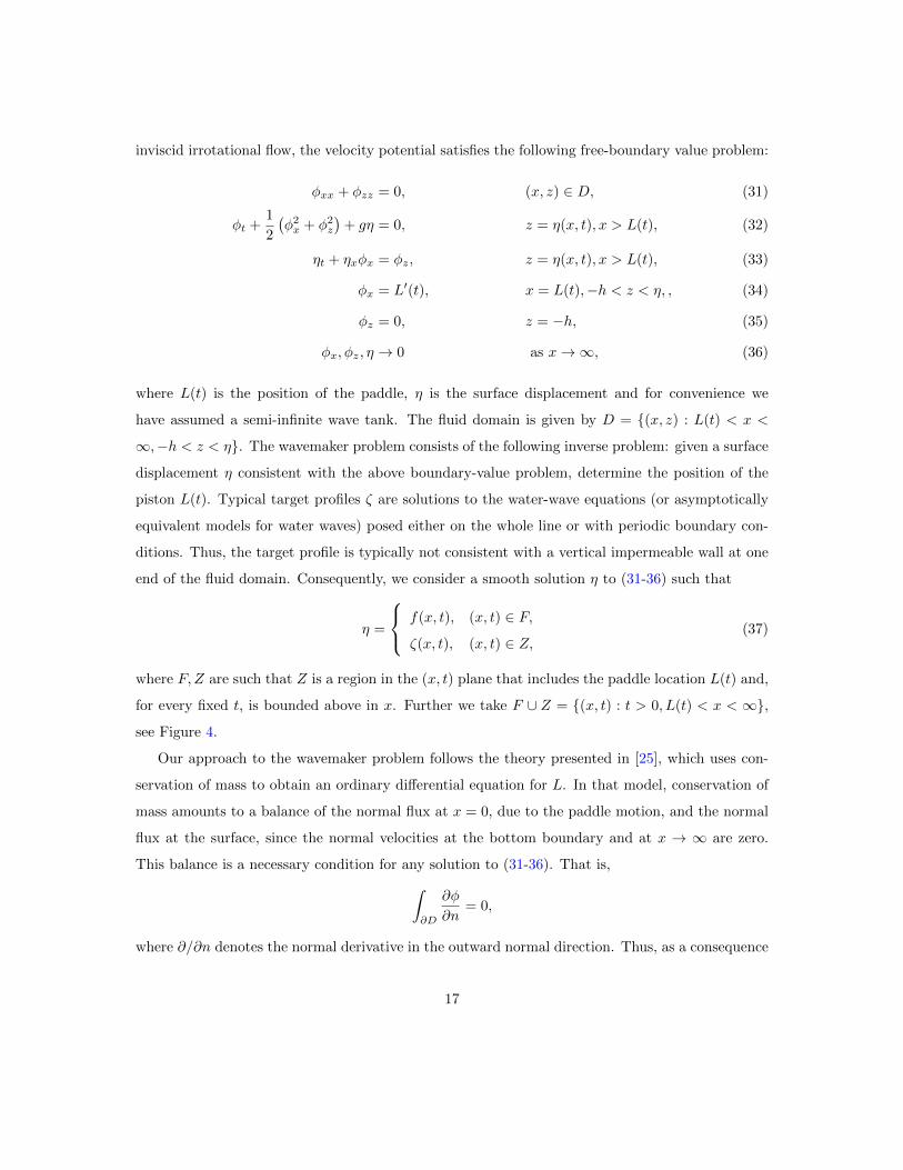
where F,Z are such that Z is a region in the (x, t) plane that includes the paddle location L(t) and,

for every fixed t, is bounded above in x. Further we take F ∪ Z = {(x, t) : t > 0, L(t) < x < ∞},see Figure 4.

Our approach to the wavemaker problem follows the theory presented in [25], which uses con-

servation of mass to obtain an ordinary differential equation for L. In that model, conservation of

mass amounts to a balance of the normal flux at x = 0, due to the paddle motion, and the normal

flux at the surface, since the normal velocities at the bottom boundary and at x → ∞ are zero.

This balance is a necessary condition for any solution to (31-36). That is,∫∂D

∂φ

∂n= 0,

where ∂/∂n denotes the normal derivative in the outward normal direction. Thus, as a consequence

17

x

t

Z

F

L(t)

Figure 4

of (33-36), we have

−L′(t)[η(L(t), t) + h] +

∫ ∞L(t)

ηt dx = 0,

⇒ dL

dt=

1

η(L(t), t) + h

∫ ∞L(t)

ηt dx. (38)

Equation (38) forms the basis for the wavemaker problem. For a given profile η, we solve the above

ordinary differential equation for L(t). In the following, we derive the associated forcing equation

for certain classes of target profiles.

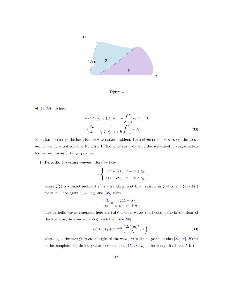
1. Periodic traveling waves: Here we take

η =

f(x− ct), x− ct ≥ ξ0,ζ(x− ct), x− ct < ξ0,

,

where ζ(ξ) is a target profile, f(ξ) is a traveling front that vanishes as ξ →∞ and ξ0 > L(t)

for all t. Once again ηt = −cηξ and (38) gives

dL

dt=

c ζ(L− ct)ζ(L− ct) + h

.

The periodic waves generated here are KdV cnoidal waves (particular periodic solutions of

the Korteweg de Vries equation), such that (see [26])

ζ(ξ) = t0 + a0cn2

(2K(m)ξ

λ,m

), (39)

where a0 is the trough-to-crest height of the wave, m is the elliptic modulus [27, 28], K(m)

is the complete elliptic integral of the first kind [27, 28], t0 is the trough level and λ is the

18

wavelength. Given a0, the frequency f0 and mean depth of fluid h, one obtains the remaining

quantities from the following relationships:

t0 =a0h

(1−m− E(m)

K(m)

),

λ = h

√16

3

mh

a0K(m),

c =√gh

[1 +

a0mh

(1− m

2− 3E(m)

2K(m)

)],

c = λf0,

where E(m) is the complete elliptic integral of the second kind [27, 28], c is the speed of the

wave and g is the acceleration due to gravity. Combining the last three equations above, one

obtains the elliptic modulus using a simple Newton’s method.

2. Reflected waves: Reflected cnoidal waves were generated when the cnoidal wave train

generated as above reached the end of the wave tank. Measurement stations for surface height

and bottom pressure were the same in the case of a single traveling wave. The reflected wave

was noted to be traveling at the same speed as the original wave however in the opposite

direction.

3. Wave group: A wave packet is produced by considering a target profile of the form ζ = ζ1+ζ2

where ζi = A sin(kix− wit). Here |w1 − w2| is small and ki is obtained by solving the linear

dispersion relation w2i = gki tanh(kih). Of course, the amplitude should be small enough such

that the linear approximation is valid. Under these assumptions, the differential equation for

L(t) has a similar form as in the previous cases, the numerator on the right-hand side being

c1ζ1 + c2ζ2 with ci = wi/ki.

5. Results

We use measurements of time series of pressure measured at a point at the bottom of the

wavetank to reconstruct the corresponding time series of the surface displacement. We compare

the reconstruction with direct measurements of the surface displacement. The theory assumes that

the wave fields are traveling waves. In previous work we showed comparisons for solitary wave

forms modeled by KdV solitons [1]. Here we look at the periodic case by generating KdV cnoidal

waves. In order to see how the theory works for more realistic shallow-water conditions, we also

19

look at wave systems outside the range of validity of the theory, including reflected cnoidal waves,

and wave groups. In the comparisons below we define the transfer function approach to be the one

obtained from linear water-wave theory. This is equivalent to (22), which is (1) with the empirical

constant N = 1.

5.1. Cnoidal wave

To look at the reconstruction for periodic waves, we generated a cnoidal wave, (39) using a

frequency of f0 = 1 Hz and crest-to-trough height of a0 = 1.9 cm in water with quiescent depth

h = 6.16 cm as discussed in §4. The speed of the cnoidal wave profile was within 0.5% of the shallow

water speed√gh, where g is the acceleration due to gravity. We note that because of dissipation

the measured wave amplitudes do not agree with the amplitude programmed at the wavemaker.

Figure 5 shows results. The measured time series is shown in Figures 5A–5C along with recon-

structions using the hydrostatic approximation (21), the transfer function (22) that accounts for

linear wave motion, and the heuristic model (23) obtained from the fully nonlinear model in [1].

We note that in the troughs, the measured time series has a bump that is not captured by the

hydrostatic or transfer functions, and only slightly captured by the heuristic model. The source

of this bump in the experiments is the contact line between the cnoidal wave crest and the glass

sidewalls. The interaction there results in a short-crested wave at symmetric angles from both

sidewalls. They intersect in the trough of the cnoidal wave and look like an inverse Kelvin wake.

Overall, we see that in this experiment, the hydrostatic approximation is the least accurate, while

the transfer and heuristic models agree reasonably well with the measurements; the heuristic model

is more accurate than the transfer function in capturing the peak amplitude. Another test of the

models is to look at their Fourier amplitudes. Figure 5D shows the ratio of predicted to measured

Fourier amplitude, with predictions from the transfer and heuristic models. An amplitude ratio of

1 corresponds to agreement between measurements and model predictions. In the reconstructions,

one must pick a wavenumber cut-off for the Fourier transforms because of the factor of cosh(kh)

that appears in the transfer function and the heuristic formula. This cut-off is clear in the ratio of

Fourier amplitudes for the transfer function (shown by the gray, dashed curve in Figure 5D) and

occurs at about 2.5 Hz. However, the nonlinearity in the heuristic formula (shown by the black,

dashed curve in Figure 5D) allows for nonlinear interactions among Fourier modes, so that it fills

in the spectrum regardless of the cut-off.

20

(A) (B)

(C) (D)

Figure 5: Reconstruction of cnoidal waves. (A-C) Time series of measured and reconstructed sur-

face displacements. Measurements are shown by the solid black curve. The dashed, gray curve

represents: (A) the hydrostatic approximation, (21); (B) the transfer function, (22); (C) the heuris-

tic formula, (23); (D) The ratio of the Fourier amplitudes of the reconstructed elevation to the

measured elevation for the transfer function (dashed, gray curve) and heuristic formula (dashed,

black curve). The solid black line shows the spectral goal of a successful reconstruction.

21

5.2. Reflected cnoidal waves

In the field, waves are reflected by beaches, other topographic features and man-made fixtures.

To see if the theory presented here, which assumes traveling waves (necessarily in one direction)

works in this regime, even though it is outside the range of validity of the theory, we did experiments

using cnoidal waves that were generated at one end of the tank, as described in §4.2 and allowed

to reflect off the wall at the other end of the tank. Below we present results for a cnoidal wave

generated with f0 = 1 Hz, a0 = 1.9 cm and h = 6.16 cm.

Figure 6 shows results. The measured time series is shown in Figure 6A–6C along with recon-

structions using the hydrostatic approximation (21), the transfer function (22) that accounts for

linear wave motion, and the heuristic model (23) obtained from the fully nonlinear model in [1].

Overall, we see that in this experiment, the hydrostatic approximation is the least accurate. The

transfer and heuristic models are in reasonable agreement with the measurements of the surface

displacements, with the heuristic formula performing best overall. As discussed in §5.1, the Fourier

amplitudes provide further information. Figure 6D shows the ratio of predicted to measured Fourier

amplitude, with predictions from the transfer and heuristic models. Again, the wavenumber cut-off

for the Fourier transforms due to the factor of cosh(kh) that appears in the transfer function and

the heuristic formula occurs at about 8 Hz. Thus, the reconstruction using the transfer function has

negligible energy in frequencies above this cut-off, while the heuristic formula, due to its allowance

for nonlinear interactions, has energy in the higher frequency modes, as does the spectrum from

the measurements.

5.3. Wave groups

When swell approaches shallow water from deep water, it typically arrives in wave groups.

Again, wave groups are outside the range of validity of the present theory, which assumes that

all waves travel at a single speed. However, we did comparisons with wave groups, which were

generated as discussed in §4.2. Here we used A = 0.5in, ω1 = 2π s−1, and ω2 = 0.1 · 2π s−1. The

results are shown in Figure 7.

All of the three models considered get the phasing of the individual waves correct. Again, the

hydrostatic approximation underestimates the wave amplitudes, while the transfer and heuristic

models are in reasonable agreement with the measurements of the surface displacements. The

heuristic formula performs best overall. As before, the spectrum shows that the nonlinear coupling

22

(A) (B)

(C) (D)

Figure 6: Reconstruction of reflected cnoidal waves. (A-C) Time series of measured and recon-

structed surface displacements. Measurements are shown by the solid black curve. The dashed,

gray curve represents: (A) the hydrostatic approximation, (21); (B) the transfer function, (22); (C)

the heuristic formula, (23); (D) The ratio of the Fourier amplitudes of the reconstructed elevation to

the measured elevation for the transfer function (dashed, gray curve) and heuristic formula (dashed,

black curve). The solid black line shows the spectral goal of a successful reconstruction.

23

of modes allowed in the heuristic formula generates energy at modes above the cut-off for analysis;

so the energy spectrum obtained from the heuristic formula is much closer to that of the measured

spectrum than is that of the transfer function.

6. Summary

We have proposed alternative formulae to the standard hydrostatic approximation and transfer

function for reconstructing a wave surface that is measured using a pressure transducer. These

formulae are approximations and extensions to the fully nonlinear, non-local formulae derived by

[1] that assumes traveling waves.The proposed formulae allow the pressure transducer to be at any

depth in the water column and can account for a uniform vorticity.

If the transducer is at the bottom of the water column, then one can approximate the water

surface displacement using the heuristic formula

η =F−1

[cosh(kh)F

[pg

]]1−F−1

[k sinh(kh)F

[pg

]] ,which is (23). If the pressure transducer is at a depth of |z0| from the still water surface, then one

first uses the pressure measurements at this depth to find the pressure at the bottom using

F [p] = sech(k(h− z0))F [p0] ,

which is (30). Then one applies the heuristic formula above given by (23). Further we extended

the fully nonlinear formulation to allow for a uniform vorticity in (A.1).

In a previous paper [1], we tested the fully nonlinear theory and various approximations with

measurements of solitons and found that, other than the fully nonlinear model, the heuristic for-

mula gave the best agreement with measurements. Here we compared reconstructions using the

hydrostatic approximation (21), the transfer function (22) and the heuristic formula (23) with mea-

surements of (periodic) cnoidal waves and with two wave systems that are outside the range of

validity of the theory: reflected cnoidal waves and wave groups. We found that since the heuris-

tic formula includes nonlinearity, its amplitude spectrum more closely approximates that of the

surface data. The hydrostatic approximation is inadequate in reconstructing the measured time

series, while both the transfer and heuristic formulae reproduce it reasonably well. Nevertheless,

24

(A) (B)

(C) (D)

Figure 7: Reconstruction of a wave group. (A-C) Time series of measured and reconstructed surface

displacements. Measurements are shown by the solid black curve. The dashed, gray curve repre-

sents: (A) the hydrostatic approximation, (21); (B) the transfer function, (22); (C) the heuristic

formula, (23); (D) The ratio of the Fourier amplitudes of the reconstructed elevation to the mea-

sured elevation for the transfer function (dashed, gray curve) and heuristic formula (dashed, black

curve). The solid black line shows the spectral goal of a successful reconstruction.

25

in a comparison of the heuristic and transfer functions, we note that the heuristic formula gives

results that are about 5% more accurate and the spectrum of the heuristic formula more accurately

describes that of the data. The heuristic formula is straightforward to use, requiring just one more

Fourier transform than the transfer function. Further the assumption of traveling waves, which is

inherent in both the heuristic formula and transfer function, does not seem to be a limiting factor

in accuracy. Thus, we conclude that the heuristic formula provides a better inverse map of pressure

measurements to surface displacement than does the transfer function.

Acknowledgments

BD and VV acknowledge support from the National Science Foundation under grant NSF-DMS-

1008001. DH acknowledges support from the National Science Foundation under grants NSF-DMS-

0708352 and NSF-DMS-1107379. KO gratefully acknowledges support from the National Science

Foundation under grant DMS-1313049 and AMS-Simons Travel Grant. We thank Robert Geist for

construction of the laboratory apparati and Rod Kreuger for building the FPGA wave gage system.

Any opinions, findings, and conclusions or recommendations expressed in this material are those of

the authors and do not necessarily reflect the views of the funding sources.

Appendix A. Reconstruction in the presence of vorticity

The basic surface reconstruction algorithm extends to the case of a two-dimensional traveling

water wave in the presence of constant vorticity. The case of a constant vorticity represents the

simplest possible situation of a wave-current interaction [29–34] and exhibits new and interesting

physical phenomena. As a result of wave-current interaction, flows develop stagnation points (where

the fluid velocity is equal to the velocity of the wave) in the interior of the fluid domain. Further,

there exist regions of the fluid where the pressure is below the atmospheric value [20, 35]. Addition-

ally, when stagnation points are present in the fluid, the maximum pressure at the bottom boundary

is no longer beneath the crest of the wave, i.e., there is a phase shift between the maximum of the

bottom pressure and the wave crest, see [20]. All these phenomena appear even when considering

constant vorticity.

In this section, we summarize the results of [20] relevant to the surface reconstruction algorithm.

For the case of solitary waves with generic vorticity, see [36]. In the following presentation, we

26

restrict to two-dimensional inviscid traveling water waves with speed c and constant vorticity γ.

The fluid motion may be described using a stream-function formulation given by

∆ψ = −γ, −h < z < η(x),

ψx = 0, at z = −h,ψ2x

2+

(ψz − c)22

+ gz − cγz + γψ =c2

2, at z = η,

(ψz − c)ηx + ψx = 0, at z = η.

As in the previous section, the horizontal boundary conditions are assumed to be either periodic or

vanishing at infinity. We normalize the stream function ψ so that ψ−cz = 0 at z = η. Consequently,

ψ(x,−h) = −m where m is the mass flow rate which we assume is a known constant. Let σs be

the sign of the horizontal fluid velocity at the free surface. We take σs = 1 to indicate a flow in

the positive x−direction in a frame relative to the wave and σs = −1 to indicate the flow in the

negative direction. Similarly, σb represents the direction of the fluid flow at the bottom boundary

z = −h. Finally, as in the irrotational case, the Bernoulli condition is valid in the bulk of the fluid

domain. As before, this permits one to translate the pressure measured at the bottom boundary

into a condition on the horizontal fluid velocity [20].

Let ϕ be the irrotational fluid stream function defined by ψ = ϕ−γz2/2+(c+σs|c|)z. Thus ϕ is

a harmonic function in the fluid domain. Further, as a consequence of the bulk Bernoulli condition

we have

ϕz(x,−h) = σb

(−|γh+ c|+

√(γh+ c)2 − 2p

),

where p is the non-static component of the bottom pressure P (x,−h), i.e.,

p = P (x,−h)/ρ− gh− γm+ γ2h2/2 + cγh.

As seen from the above expression, we require m, σs, σb, γ and c to define the non-static pressure

and the fluid velocity at the bottom boundary. Having defined these quantities, the analysis follows

that used to obtain (19). We simply state the associated nonlinear nonlocal expression for the

surface profile.

σs

(−|c|+

√c2 − 2gη

1 + η2x

)=σb2π

∫ ∞−∞

eikx cosh(k(η + h))F{−|γh+ c|+

√(γh+ c)2 − 2p

}(k)dk.

(A.1)

27

We note that, for nontrivial flows with γ = 0, no stagnation points exist within the fluid and thus

σs = σb. Consequently, (A.1) reduces to (19) in this case.

[1] K. Oliveras, V. Vasan, B. Deconinck, D. Henderson, Recovering the water-wave profile from

pressure measurements, SIAM J. Appl. Math. 72 (2012) 897–918.

[2] G. Stokes, Mathematical and Physical Papers, Vol. 1, Johnson Reprint Corp. NY &

London, 1966.

[3] U. A. E. W. E. Station, Shore Protection Manual, Vol. 1m 4th ed, Vicksburg Miss MI, 1984.

[4] C. T. Bishop, M. A. Donelan, Measuring waves with pressure transducers, Coastal Engineering

11 (1987) 309–328.

[5] D. Y. Lee, H. Wang, Measurement of surface waves from subsurface guage, 1984.

[6] A. O. Bergan, A. Torum, A. Traetteberg, Wave measurements by pressure type wave gauge,

Proc. 11th Coastal Eng. Cong. ASCE (1968) 19–29.

[7] C.-H. Tsai, M.-C. Huang, F.-J. Young, Y.-C. Lin, H.-W. Li, On the recovery of surface wave

by pressure transfer function, Ocean Engineering 32 (2005) 1247–1259.

[8] J.-Y. Chen, Three dimensional nonlinear pressure transfer function, Coastal Engineering 11111

(2000) 3111109–3111128.

[9] Y. Y. Kuo, Y. F. Chiu, Transfer function between the wave height and wave pressure for

progressive waves, Coastal Engineering 23 (1994) 81–93.

[10] A. Baquerizo, M. A. Losada, Transfer function between wave height and wave pressure for

progressive waves, by Y.-Y. Kuo and J.-F. Chiu: comments, Coastal Engineering 24 (1995)

351–353.

[11] Y. Y. Kuo, Y. F. Chiu, Transfer function between the wave height and wave pressure for

progressive waves: reply to the comments of a. baquerizo and m. a. losada, Coastal Engineering

24 (1995) 355–356.

[12] D. Clamond, A. Constantin, Recovery of steady periodic wave profiles from pressure measure-

ments at the bed, J. Fluid Mech. 714 (2013) 463–475.

28

[13] A. Constantin, On the recovery of solitary wave profiles from pressure measurements, J. Fluid

Mech. 699 (2012) 1–9.

[14] H.-C. Hsu, Recovering surface profiles of solitary waves on a uniform stream from pressure

measurements, DCDS-A 34 (2014) 3035–3043.

[15] D. Clamond, New exact relations for easy recovery of steady wave profiles from bottom pressure

measurements, J. Fluid Mech. 726 (2013) 547–558.

[16] J.-C. Tsai, C.-H. Tsai, H.-M. Tseng, Pressure derived wave height using artificial neural net-

works, Proc Oceans’08 MTS/IEEE Kobe-Techno-Ocean (2008) 1–8.

[17] J.-C. Tsai, C.-H. Tsai, Wave measurements by pressure transducers using artificial neural

networks, Ocean Engineering 36 (2009) 1149–1157.

[18] A. B. Kennedy, R. Gravois, B. Zachry, R. Luettich, T. Whipple, R. Weaver, J. Reynolds-

Fleming, Q. J. Chen, R. Avissar, Rapidly installed temporary gauging for hurrican waves and

surge, and application to hurricane gustav, Continental Shelf Research 30 (2010) 1743–1752.

[19] M. J. Ablowitz, A. S. Fokas, Z. H. Musslimani, On a new non-local formulation of water waves,

J. Fluid Mech. 562 (2006) 313–343.

[20] V. Vasan, K. L. Oliveras, Pressure beneath a traveling wave with constant vorticity, Disc. &

Cont. Dyn. Sys. Ser. 34 (2014) 3219–3239.

[21] K. L. Oliveras, V. Vasan, Relationships between the pressure and the free surface independent

of the wave speed, Contemporary Mathematics 635 (2015) 157–173.

[22] B. Deconinck, K. L. Oliveras, V. Vasan, Relating the bottom pressure and the surface elevation

in the water wave problem, J. Nonlinear Math. Phys. 19 (suppl. 1) (2012) 1240014, 11.

[23] A. Constantin, W. Strauss, Pressure and trajectories beneath a Stokes wave, Communications

on Pure and Applied Mathematics 63 (2010) 533–557.

[24] B. Deconinck, K. Oliveras, The instability of periodic surface gravity waves, J. Fluid Mech.

675 (2011) 141–167.

29

[25] D. G. Goring, F. Raichlen, The generation of long waves in the laboratory, Proc. 17th Intl.

Conf. Coastal Engrs., Sydney, Australia 11111 (1980) 3111109–3111128.

[26] M. W. Dingemans, Water Wave Propagation Over Uneven Bottoms, World Scientific, 1997.

[27] NIST Digital Library of Mathematical Functions, http://dlmf.nist.gov/, Release 1.0.9 of 2014-

08-29, online companion to [28].

URL http://dlmf.nist.gov/

[28] F. W. J. Olver, D. W. Lozier, R. F. Boisvert, C. W. Clark (Eds.), NIST Handbook of Math-

ematical Functions, Cambridge University Press, New York, NY, 2010, print companion to

[27].

[29] A. Constantin, W. Strauss, Exact steady periodic water waves with vorticity, Communications

on Pure and Applied Mathematics 57 (2004) 0481–0527.

[30] A. Constantin, W. Strauss, Rotational steady water waves near stagnation, Phil. Trans. R.

Soc. A. 356 (2007) 2227–2239.

[31] E. Wahlen, Steady periodic capillary waves with vorticity, Ark. Mat. 44 (2006) 367–387.

[32] E. Wahlen, Steady water waves with a critical layer, J. Diff. Eq. 246 (2009) 2468–2483.

[33] J. Ko, W. Strauss, Effect of vorticity on steady water waves, J. Fluid Mech. 608 (2008) 197–216.

[34] J. Ko, W. Strauss, Large-amplitude steady rotational water waves, Eur. J. Mech. B/Fluids

27 (2) (2008) 96–109.

[35] A. T. D. Silva, D. H. Peregrine, Steep, steady surface waves on water of finite depth with

constant vorticity., J. Fluid Mech. 195 (1988) 281–302.

[36] D. Henry, On the pressure transfer function for solitary water waves with vorticity, Math. Ann.

(2013) 1–8.

30