A Methodology for Determining the Return on Investment ...escml.umd.edu/Papers/Feldman_et_al_IEEE_Trans_Rel.pdf · Investment (ROI) for PHM activities, and presents a study conducted

IEEE Trans. on Reliability, Vol. 58, No. 2, pp. 305-316, June 2009

1

A Methodology for Determining the Return on Investment Associated with Prognostics and Health Management

Kiri Feldman, Member, IEEE, Taoufik Jazouli, and Peter Sandborn, Senior Member, IEEE CALCE Center for Advanced Life Cycle Engineering

Department of Mechanical Engineering University of Maryland, College Park, MD 20742

Abstract—Prognostics and Health Management (PHM) provides opportunities for lowering sustainment

costs, improving maintenance decision-making, and providing product usage feedback into the product

design and validation process. However, support for PHM is predicated on the articulation of clear business

cases that quantify the expected cost and benefits of its implementation. The realization of PHM requires

implementation at different levels of scale, and complexity. The maturity, robustness, and applicability of the

underlying predictive algorithms impact the overall efficacy of PHM within an enterprise. The utility of

PHM to inform decision-makers within tight scheduling constraints, and under different operational profiles

likewise affects the cost avoidance that can be realized. This paper discusses the calculation of Return on

Investment (ROI) for PHM activities, and presents a study conducted using a stochastic discrete event

simulation model to determine the potential ROI offered by electronics PHM. The case study of a

multifunctional display in a Boeing 737 compares the life cycle costs of a system employing unscheduled

maintenance to the same system using a precursor to failure PHM approach.

Index Terms—Avionics, cost modeling, electronics prognostics and health management, prognostics and

health management, return on investment.

ACRONYM1

CALCE Center for Advanced Life Cycle Engineering

CBA Cost Benefit Analysis

DoD Department of Defense


2

FAA Federal Aviation Administration

FMECA Failure Modes, Effects, and Criticality Analysis

HM Health Monitoring

JSF Joint Strike Fighter

LAV Light Armored Vehicle

LCOM Logistics Composite Model

LRU Line Replaceable Unit

MFD Multifunction Display

MRO Maintenance, Repair, and Overhaul

NASA National Aeronautics and Space Administration

OMB Office of Management and Budget

PHM Prognostics and Health Management

RUL Remaining Useful Life

ROI Return On Investment

SBCT Stryker Brigade Combat Team

TTF Time To Failure

NOTATION

β Weibull shape parameter

Cassembly Cost of assembly and installation of the hardware in each LRU or the cost of assembly of PHM hardware

for each socket or for each group of sockets

Cdata Cost of data management, including the costs of data archiving, data collection, data analysis, and data

reporting

Cdecision Cost of decision support

Cdev_hard Cost of hardware development

Cdev_soft Cost of software development

1 The singular and plural of an acronym are always spelled the same.


3

Cdoc Cost of documentation

Chard_add Cost of PHM hardware added to each LRU (e.g., sensors, chips, extra board area), and may include the

cost of additional parts or manufacturing, or the cost of hardware for each socket (such as connectors, and

sensors)

CINF Infrastructure costs associated with the application and support of PHM

Cinstall Cost of installation of PHM hardware for each socket or for each group of sockets, which includes the

original installation, and re-installation upon failure, repair, or diagnostic action

Cint Cost of integration

CLRU i Cost of procuring a new LRU for socket i

CLRU repair i Cost of repairing an LRU in socket i

CNRE PHM non-recurring costs

CPHM Total life cycle cost of the system employing a particular PHM approach

Cprognostic maintenance Cost of maintenance of the prognostic devices

Cqual Cost of testing, and qualification

CREC PHM recurring costs

Cretraining Cost of retraining to educate personnel in the use of PHM

Csocket i Life cycle cost of socket i

Ctest Cost of recurring functional testing of PHM hardware for each socket or for each group of sockets

Ctraining Cost of training

Cus Total life cycle cost of the system when managed using an unscheduled maintenance policy

d Prognostic distance

f Fraction of maintenance events on a socket that require replacement of the LRU in the socket with a new

LRU

γ Weibull location parameter

IPHM Total investment in the PHM approach

Ius Total investment in the unscheduled maintenance policy

η Weibull scale parameter


4

r Discount rate

t Year of event (t = 0 corresponds to 2008)

t1 TTF distribution sample

Trepair i Time to repair the LRU in socket i

Treplace i Time to replace the LRU in socket i

V Value of time out of service


5

I. INTRODUCTION

All Prognostics and Health Management (PHM) approaches are essentially the extrapolation of trends based on

recent observations to estimate Remaining Useful Life (RUL) [1]. The value obtained from PHM can take the form

of advanced warning of failures; increased availability through extensions of maintenance cycles or timely repair

actions; lower life cycle costs of equipment from reductions in inspection costs, downtime, inventory, and no-fault-

founds; or the improvement of system qualification, design, and logistical support of fielded and future systems [2].

Proposals to adopt PHM approaches are often articulated in the form of business cases; an economic justification is

the cornerstone of a persuasive case. Return on Investment (ROI) is a useful means of gauging the economic merits

of adopting PHM.

The determination of the ROI allows managers to include quantitative, readily interpretable results in their

decision-making. ROI analysis may be used to select between different types of PHM, to optimize the use of a

particular PHM approach, or to determine whether to adopt PHM versus more traditional maintenance approaches.

The economic justification of PHM has been discussed by many authors [3]-[21]. Although the existing PHM

ROI assessments described in this section contain valuable insight into the cost drivers, most PHM cost analyses

and cost-benefit analyses are application-specific; in most cases, they do not provide a general modeling framework

or consistent process with which to evaluate the application of PHM to a system. Furthermore, existing approaches

provide primarily ‘point estimates’ of the value based on a set of fixed inputs when, in reality, many of the critical

inputs are uncertain. Accommodating the uncertainties in the PHM ROI calculation is at the heart of developing

realistic business cases that address prognostic requirements. Finally, for many types of systems, the value of PHM

is realized through the changes it enables in the ability to maintain the system. While the models in [3]-[20] all

contain cost factors associated with maintenance, most neither simulate nor emulate the maintenance process. The

work described in this paper is based on modeling PHM within the maintenance planning tool described in [21],

using a detailed treatment of the maintenance process to gain a more accurate understanding of the true value of

PHM.

The ROI associated with PHM approaches has been examined for specific non-electronic military applications,

including ground vehicles, power supplies, and engine monitors [3]-[5]. NASA studies indicate that the ROI of


6

prognostics in aircraft structures may be as high as 0.58 in 3 years for contemporary and older generation aircraft

systems assuming a 35% reduction in maintenance requirements [6]. Simple ROI analyses of electronic prognostics

for high reliability telecommunications applications (power supplies, and power converters) have been conducted,

including a basic business case for the BladeSwitch voice telecommunications deployment in Malaysia [7].

ROI predictions of the costs of PHM implementation, and the potential for cost avoidance have been evaluated;

and an analysis of PHM for JSF aircraft engines was developed using a methodology that employed Failure Modes,

Effects, and Criticality Analysis (FMECA) to model hardware [8], [9]. Byer et al. [10], and Leao et al. [11]

describe processes for conducting a cost-benefit analysis for prognostics applied to aircraft subsystems.

The cost-benefit analysis of PHM for batteries within ground combat vehicles was modeled using the Army

Research Laboratory’s Trade Space Visualizer software tool [12]. Banks & Merenich [12] found that ROI was

maximized when the time horizon (the prognostic distance) was greatest, and when the number of vehicles and the

failure rates were largest. A comparison of the ROI of prognostics for two types of military ground vehicle

platforms was performed using data from Pennsylvania State University’s battery prognostics program [13]. Non-

recurring development costs were estimated for the prognostic units developed for the batteries of the Light

Armored Vehicle (LAV), and the Stryker platform used in the Stryker Brigade Combat Team (SBCT) family of

vehicles. ROI was calculated as 0.84 for the LAV, and 4.61 for the SBCT based on estimates of the development

and implementation costs. When combined with existing data about battery performance across the Department of

Defense (DoD), the total ROI of battery prognostics for the DoD was calculated as 15.25 over a 25-year period.

The Boeing Company developed a life cycle cost model for evaluating the benefits of prognostics for the Joint

Strike Fighter program. The model was developed by Boeing’s Phantom Works division to enable cost-benefit

analysis of prognostics for the fighter’s avionics during system demonstration, and then enhanced to permit life

cycle cost assessment of prognostic approaches [14]. Cost influencing parameters, in addition to economic factors,

were incorporated into a cost benefit analysis [15].


7

II. PROPOSED METHODOLOGY OF RETURN ON INVESTMENT (ROI) CALCULATION

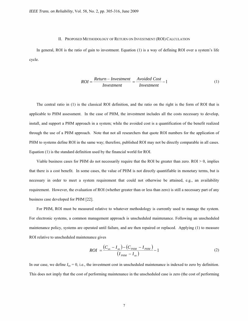
In general, ROI is the ratio of gain to investment. Equation (1) is a way of defining ROI over a system’s life

cycle.

Investment

InvestmentReturn ROI −= 1

−=Investment

CostAvoided (1)

The central ratio in (1) is the classical ROI definition, and the ratio on the right is the form of ROI that is

applicable to PHM assessment. In the case of PHM, the investment includes all the costs necessary to develop,

install, and support a PHM approach in a system; while the avoided cost is a quantification of the benefit realized

through the use of a PHM approach. Note that not all researchers that quote ROI numbers for the application of

PHM to systems define ROI in the same way; therefore, published ROI may not be directly comparable in all cases.

Equation (1) is the standard definition used by the financial world for ROI.

Viable business cases for PHM do not necessarily require that the ROI be greater than zero. ROI > 0, implies

that there is a cost benefit. In some cases, the value of PHM is not directly quantifiable in monetary terms, but is

necessary in order to meet a system requirement that could not otherwise be attained, e.g., an availability

requirement. However, the evaluation of ROI (whether greater than or less than zero) is still a necessary part of any

business case developed for PHM [22].

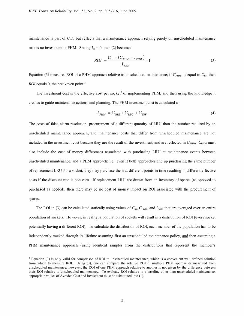
For PHM, ROI must be measured relative to whatever methodology is currently used to manage the system.

For electronic systems, a common management approach is unscheduled maintenance. Following an unscheduled

maintenance policy, systems are operated until failure, and are then repaired or replaced. Applying (1) to measure

ROI relative to unscheduled maintenance gives

( ) ( )( ) 1−

−−−−

=usPHM

PHMPHMusus

IIICIC

ROI (2)

In our case, we define Ius = 0, i.e., the investment cost in unscheduled maintenance is indexed to zero by definition.

This does not imply that the cost of performing maintenance in the unscheduled case is zero (the cost of performing


8

maintenance is part of Cus), but reflects that a maintenance approach relying purely on unscheduled maintenance

makes no investment in PHM. Setting Ius = 0, then (2) becomes

( )1−

−−=

PHM

PHMPHMus

IICC

ROI (3)

Equation (3) measures ROI of a PHM approach relative to unscheduled maintenance; if CPHM is equal to Cus, then

ROI equals 0, the breakeven point.2

The investment cost is the effective cost per socket3 of implementing PHM, and then using the knowledge it

creates to guide maintenance actions, and planning. The PHM investment cost is calculated as

INFRECNREPHM CCCI ++= (4)

The costs of false alarm resolution, procurement of a different quantity of LRU than the number required by an

unscheduled maintenance approach, and maintenance costs that differ from unscheduled maintenance are not

included in the investment cost because they are the result of the investment, and are reflected in CPHM. CPHM must

also include the cost of money differences associated with purchasing LRU at maintenance events between

unscheduled maintenance, and a PHM approach; i.e., even if both approaches end up purchasing the same number

of replacement LRU for a socket, they may purchase them at different points in time resulting in different effective

costs if the discount rate is non-zero. If replacement LRU are drawn from an inventory of spares (as opposed to

purchased as needed), then there may be no cost of money impact on ROI associated with the procurement of

spares.

The ROI in (3) can be calculated statically using values of Cus, CPHM, and IPHM that are averaged over an entire

population of sockets. However, in reality, a population of sockets will result in a distribution of ROI (every socket

potentially having a different ROI). To calculate the distribution of ROI, each member of the population has to be

independently tracked through its lifetime assuming first an unscheduled maintenance policy, and then assuming a

PHM maintenance approach (using identical samples from the distributions that represent the member’s

2 Equation (3) is only valid for comparison of ROI to unscheduled maintenance, which is a convenient well defined solution from which to measure ROI. Using (3), one can compare the relative ROI of multiple PHM approaches measured from unscheduled maintenance; however, the ROI of one PHM approach relative to another is not given by the difference between their ROI relative to unscheduled maintenance. To evaluate ROI relative to a baseline other than unscheduled maintenance, appropriate values of Avoided Cost and Investment must be substituted into (1).


9

characteristics and maintenance costs in a Monte Carlo analysis). In this manner, a separate ROI is calculated for

each member of the population. When the process is repeated on an entire population of sockets, a histogram of

ROI is generated from which business case parameters can be extracted. For the example in Fig. 7 (discussed later),

assuming that the estimation of the uncertainties in the input parameters is reasonable, the case study in Section IV

indicates that we can have 80% confidence that the ROI is greater than 3.12.

III. PHM COSTS

The two major categories of cost-contributing activities that must be considered in an analysis of the ROI of

PHM are implementation costs, and cost avoidance. These categories represent the ‘Investment’ portion, and the

‘Avoided Cost’ portion of the ROI calculation in (1) respectively.

A. Implementation Costs

Implementation costs are the costs associated with the realization of PHM in a system, the technologies and

support necessary to integrate and incorporate PHM into new or existing systems. The costs of implementing PHM

can be categorized as recurring, non-recurring, or infrastructural depending on the frequency, and role of the

corresponding activities. The implementation cost is the cost of enabling the determination of Remaining Useful

Life (RUL) for the system.

Non-recurring costs are associated with one-time only activities that typically occur at the beginning of the

timeline of a PHM program, although disposal or recycling non-recurring costs would occur at the end. Non-

recurring costs can be calculated on a per-LRU, per-socket, or per a group of LRU or sockets basis. The specific

non-recurring cost is calculated as

qualdoctrainingdev_softdev_hardNRE CCCCCCC +++++= int (5)

Recurring costs are associated with activities that occur continuously or regularly during the PHM program. As

with non-recurring costs, some of these costs can be viewed as an additional charge for each instance of a LRU, or

for each socket (or for a group of LRU or sockets). The recurring cost is calculated as

3 A socket is a unique instance of an installation location for an LRU. One instance of a socket occupied by an engine controller is its location on a particular engine. The socket may be occupied by a single LRU during its lifetime (if the LRU never fails), or


10

installtestassemblyhard_addREC CCCC C +++= (6)

Unlike recurring and non-recurring costs, infrastructure costs are associated with the support features and

structures necessary to sustain PHM over a given activity period, and are characterized in terms of the ratio of

money to a period of activity (i.e., dollars per operational hour, dollars per mission, dollars per year). The

infrastructure costs are calculated as

CINF = Cprognostic maintenance + Cdecision + Cretraining + Cdata (7)

B. Cost Avoidance

Prognostics provide estimations of Remaining Useful Life (RUL) in terms that are useful to the maintenance

decision making process. The decision process can be tactical (real-time interpretation and feedback), or strategic

(maintenance planning, or feedback into the product design or verification process). Unfortunately, the calculation

of RUL alone does not provide sufficient information to form a decision, or to determine corrective action.

Determining the best course of action requires the evaluation of criteria such as availability, reliability,

maintainability, and life cycle cost. Cost avoidance is the value of changes to availability, reliability,

maintainability, and failure avoidance.

The primary opportunities for obtaining cost avoidance from the application of PHM to systems are failure

avoidance, and minimization of the loss of remaining system life. Field failure of systems is often very expensive.

If all or some fraction of the field failures can be avoided, then cost avoidance may be realized by minimizing the

frequency of unscheduled maintenance. Avoidance of failures can increase availability, reduce the risk of loss of

the system, and may increase human safety depending on the type of system considered. Failures avoided fall into

two types: 1) real-time failure avoidance during operation that would otherwise result in the loss of the system or

loss of the function that the system was performing (i.e., loss of mission), and 2) warning of future (but not

imminent) failure that allows preventative maintenance to be performed at a convenient place and time.

multiple LRU if one or more LRU fail, and needs to be replaced.


11

C. Maintenance Planning Cost Model

Interpretation of RUL results from PHM activities is a decision making under uncertainty problem. Without

comprehending the corresponding measures of the uncertainty associated with the calculation, RUL projections

have little practical value, [1]. To perform effective maintenance planning, and calculate corresponding life cycle

costs, we must use a method that includes data uncertainties. We use a stochastic discrete event simulation model

[21] to compute the total life cycle cost of sockets when unscheduled, and PHM management approaches are used;

i.e., we compute Cus and CPHM in (3). The model follows the history of a single socket (or a group of sockets) from

time zero to the end of support life for the system. To generate meaningful results, a s-relevant number of sockets

(or systems of sockets) are modeled, and the resulting cost and other metrics are generated in the form of

histograms. The model treats all inputs to the discrete event simulation as probability distributions, i.e., a stochastic

analysis is used, implemented as a Monte Carlo simulation. Various maintenance interval and PHM approaches are

distinguished by how sampled TTF values are used to model PHM RUL forecasting distributions.

The case study in this paper focuses on a Precursor to Failure PHM approach, and includes maintenance

planning model details for this PHM approach. The treatment of other PHM approaches appears in detail in [21].

Precursor to failure monitoring employs fuses or other monitored structures that are manufactured with or within the

LRU, or as monitored precursor variables representing non-reversible physical processes, i.e., they are coupled to

the manufacturing, material, or assembly variations of a particular LRU. Health Monitoring (HM), and LRU-

dependent fuses are examples of precursor to failure methods. A parameter to be determined from the analysis is the

prognostic distance. The prognostic distance is a measure of how long before system failure the prognostic

structures or prognostic cell is expected to indicate failure. The precursor to failure monitoring methodology

forecasts a unique time to failure (TTF) distribution for each instance of an LRU based on the instance’s TTF.4 For

illustration purposes, the precursor to failure monitoring forecast is represented as a symmetric triangular

distribution with a most likely value (mode) set to the TTF of the LRU instance, minus the prognostic distance, Fig.

1.5

4 In this model, all failing LRU are assumed to be maintained via replacement or good-as-new repair. Therefore, the time between failure, and the time to failure are the same. 5 Luna [23] has suggested a generalization of the model used in [21], and describes its possible implementation within the Logistics Composite Model (LCOM) developed for the Air Force, [24]. Similar to the model in [21], LCOM is a discrete event simulation based operation and maintenance models.


12

The LRU TTF probability density function (pdf), and the precursor to failure TTF pdf on the left, and right

sides of Fig. 1, respectively, could have different distribution shapes and parameters; symmetric triangular

distributions were chosen for illustration. The precursor to failure monitoring distribution has a fixed width

measured in the relevant environmental stress units (e.g., operational hours in our example) representing the

probability of the prognostic structure indicating the precursor to a failure. As a simple example, if the prognostic

structure was a LRU-dependent fuse that was designed to fail at some prognostic distance earlier than the system it

protects, then the distribution on the right side of Fig. 1 represents the distribution of fuse failures (the TTF

distribution of the fuse).

The model proceeds in the following way: for each LRU TTF distribution sample (t1) taken from the left side of

Fig. 1, a precursor to failure monitoring TTF distribution is created that is centered on the LRU TTF minus the

prognostic distance (t1-d). The precursor to failure monitoring TTF distribution is then sampled, and if the precursor

to failure monitoring TTF sample is less than the actual TTF of the LRU instance, the precursor to failure

monitoring is deemed successful. If the precursor to failure monitoring distribution TTF sample is greater than the

actual TTF of the LRU instance, then precursor to failure monitoring was unsuccessful. If successful, a scheduled

maintenance activity is performed, and the timeline for the socket is incremented by the precursor to failure

monitoring sampled TTF. If unsuccessful, an unscheduled maintenance activity is performed, and the timeline for

the socket is incremented by the actual TTF of the LRU instance. At each maintenance activity, the relevant costs

are accumulated.

The scheduled, and unscheduled costs computed for the sockets at each maintenance event are given by

Vf)T(+VfT+f)C(+fC=C irepairireplaceirepairLRUiLRUisocket −− 11

(8)

Note that the values of f, and V generally differ depending on whether the maintenance activity is scheduled or

unscheduled. For simplicity, (8) is written assuming that the quantity of replaced LRU in socket i is one; however,

the socket could receive multiple LRU during its lifetime.

As the discrete event simulation tracks the actions that affect a particular socket during its life cycle, the

implementation costs are charged at the appropriate times, as shown in Fig. 2. At the beginning of the life cycle, the

non-recurring cost is applied. The recurring costs at the LRU level, and at the system level are first applied at the

start of the analysis; and, assuming spares are procured as needed, they are subsequently applied at each


13

maintenance event that requires replacement of an LRU (CLRU i, as in (8)). The recurring LRU-level costs include

the base cost of the LRU regardless of the maintenance approach. Discrete event simulations that compare

alternative maintenance approaches to determine the ROI of PHM must include the base cost of the LRU itself

without any PHM-specific hardware. If discrete event simulation is used to calculate the life cycle cost for a socket

under an unscheduled maintenance policy, then the recurring LRU-level cost is reduced to the cost of replacing or

repairing an LRU upon failure. Under a policy involving PHM, the failure of an LRU results in additional costs for

the hardware, assembly, and installation of the components used to perform PHM. The infrastructure costs are

distributed over the socket’s life cycle.

The maintenance planning simulation can be performed assuming that spares can be purchased as needed, or

that spares reside in an inventory. The spares inventory model includes the purchase of an initial quantity of spares

(the purchase is assumed to happen at the start of the simulation), and an inventory carrying cost is assessed per year

based on the number of spares that reside in the inventory at the beginning of the year. When the number of spares

in the inventory drops below a user defined threshold, additional spares are automatically purchased, and become

available in the inventory for use after a user definable lead-time. Cost of money is assessed on all spares

purchases, inventory, and replenishment activities.

IV. CASE STUDY

The scenario for this business case example considers the acquisition of a precursor to failure PHM approach

for an avionics LRU in a commercial aircraft used by a major commercial airline. The representative LRU is a

multifunction display (MFD), two of which are present in each aircraft. A fleet size of 502 aircraft was chosen to

reflect the quantities involved for a technology acquisition by a major airline, in this case, Southwest Airlines [25].

The Boeing 737-300 series was chosen as the representative aircraft to be equipped with electronics PHM. A

preliminary version of this case study appeared in [26].

The implementation costs reflect a composite of technology acquisition cost benefit analyses (CBA) for aircraft,

and/or for prognostics. The implementation costs are summarized in Table I. All values are in 2008 U.S. dollars; all

conversions to year 2008 dollars were performed using the Office of Management and Budget (OMB) discount rate


14

of 7% [27]. The discount factor was calculated as 1/(1 + r)t, where r is the discount rate (0.07), and t is the year (t =

0 represents 2008).

Maintenance costs vary greatly depending on the type of aircraft, the airline, the amount and extent of

maintenance needed, the age of the aircraft, the skill of the labor base, and the location of the maintenance

(domestic versus international, hangar versus special facility). The maintenance costs in the model are assumed to

be fixed; however, the effects of aging are known to increase maintenance costs [28].

Koch, et al. [29] give the maintenance cost per hour for Boeing 737-100 and -200 series aircraft as 12% of the

hourly operating cost, noting that the ratio of maintenance costs per hour to aircraft operating costs per hour has

remained between 0.08, and 0.13 since the 1970s. The numerical average of the direct hourly operating costs for

major airlines summarized in [30] was used. This cost is treated as the cost of scheduled maintenance per hour,

which is equivalent to the cost of unscheduled maintenance that can be performed during the downtime period (see

Table II) after the flight segments for the day have been completed.

The cost of unforeseen failures that require immediate attention during a flight can vary depending on the

interpretation, and on the subsequent actions required to correct the problem. Unscheduled maintenance that would

require a diversion of a flight can be extremely expensive. The cost of a problem requiring unscheduled

maintenance that is detected before the aircraft has left the ground (during a flight segment but not airborne) can be

highly complex to model if the full value of passenger delay time, and the downstream factors of loss of reputation

and indirect costs are included [31].

For the determination of the cost of unscheduled maintenance during a flight segment, we assume that such an

action typically warrants a flight cancellation. This represents a more extreme scenario than a delay; the model

assumes that unscheduled maintenance that occurs between flight segments (during the preparation and turnaround

time) would be more likely to cause a delay, whereas unscheduled maintenance during a flight segment would result

in a cancellation of the flight itself. The Federal Aviation Administration (FAA) provides average estimates of the

cost of cancelled flights on commercial passenger aircraft based on direct operating costs per minute [32].

The operational profile for this example case was determined by gathering information for the flight frequency

of a typical commercial aircraft. A large aircraft is typically flown several times each day; these individual journeys

are known as flight segments. The average number of flight segments for a Southwest Airlines aircraft was seven in


15

2007 [25]. Although major maintenance, repair, and overhaul operations (MRO) call for lengthy periods of

extensive inspections and upgrades as part of mandatory maintenance checks, a commercial aircraft may be

expected to be operational up to 90% to 95% of the time for a given year [33]. A median airborne time for

commercial domestic flights was approximately 125 minutes in 2001 [27]. A representative support life of 20 years

was chosen based on [27]. A 45-minute turnaround time was taken as the time between flights based on the industry

average [34]. Using this information, an operational profile was constructed whose details are summarized in Tables

II, and III.

Table IV summarizes the spares inventory assumptions made for the maintenance model. As an alternative,

results are also provided in this section for the assumption that replacement spares can be acquired, and paid for as

needed (no spares inventory, and no lead-time for obtaining replenishment spares, i.e., all costs associated with

maintaining an inventory of spares are assumed to be incorporated into the LRU recurring cost).

Reliability data were based on [35], and [36], which provide models of the reliability of avionics with

exponential, and Weibull distributions, commonly used to model avionics [37]. The assumed TTF distribution of

the LRU is provided on the left side of Fig. 3 (i.e., ‘TTF 1’). In an analysis of over 20,000 electronic products built

in the 1980s and 1990s, [38] shows that Weibull distributions with shape parameters close to 1, i.e., close to the

exponential distribution, are the most appropriate Weibull distributions for modeling avionics. Upadhya &

Srinivasan [39] model the reliability of avionics with a Weibull shape parameter of 1.1, consistent with the common

range of parameters found in [38]. Although [38] found exponential distributions to be the most accurate, failure

mechanisms associated with current technologies suggest that the Weibull may prove to be more representative for

future generations of electronic products [40]. The location parameter was chosen based on the typical avionics unit

being considerably shorter-lived than the ten-year lifespan commonly used within the aerospace industry [38]. The

right side of Fig. 3 (‘TTF 2’) provides an alternative TTF distribution that was used for comparison.

A. ROI Analysis

In this section, the ROI of a precursor to failure PHM approach relative to unscheduled maintenance is

analyzed for four cases: with, and without a spares inventory for each of the two different TTF distribution

assumptions (TTF 1, and TTF 2) as shown in Fig. 3. The cases without spares inventories correspond to the


16

assumption that spares are purchased and available to be procured without delay whenever they are needed. Only a

precursor to failure PHM approach is considered in this case study.

To enable the calculation of ROI, an analysis proceeds along the steps shown in Fig. 4. The results of the

analysis to determine the optimal prognostic distance when using precursor to failure PHM for the example case are

shown in Fig. 5. Small prognostics distances cause PHM to miss failures, while large distances are overly

conservative. For the combination of PHM approach, implementation costs, reliability information, and operational

profile assumed in this example, a prognostic distance of 470 hours for TTF 1 yielded the minimum life cycle cost

over the support life. A symmetric triangular distribution with a width of 500 hours was assumed for the TTF

distribution of the prognostic structure that was monitored with the precursor to failure approach (the right side of

Fig. 1). Similarly, the optimum prognostic distance using TTF 2 was 500 hours. Note that a 12 month lead time for

spare replenishment (as defined in Table IV) was assumed in Figs. 5-8.

Using prognostic distances of 470 and 500 hours, a discrete event simulation was performed under the

assumptions of negligible random failure rates, and false alarm indications. Fig. 6 illustrates the cumulative cost per

socket as a function of time. The graph of life cycle cost intersects the ordinate axis at the point corresponding to the

initial implementation cost (including the initial spares inventory if applicable); as maintenance events accumulate

over the support life, the cost rises, culminating at the end of the 20 years. For the case where LRU can be procured

as needed (i.e., no spares inventory, the left side of Fig. 6), each socket required a replacement of five LRU on

average, corresponding to the distinct steps in cost every ~3.8 years. The small step increases between LRU

replacements (most clearly seen between year 0, and year 3) represent annual PHM infrastructure costs. For this

case study, 1,000 sockets were simulated; divergence in life cycle cost due to randomness and variability of

parameters can be seen as the support life progresses. When a spares inventory (defined in Table IV) is assumed

(on the right side of Fig. 6), the threshold for spare replenishment is reached between years 11 and 13, resulting in

the purchase of 2 additional spares per socket. This result corresponds to the single large step appearing in the plot

on the right side of Fig. 6; the initial cost is larger than that on the left because of the cost of the initial spares

inventory.

Using the PHM approach, 99% of the failures were avoided for both the no spares inventory, and spares


17

inventory cases respectively.6 The total life cycle cost per socket was CPHM = $77,338 in the no spares inventory

case, and $234,587 when a spares inventory was included, with effective investment costs per socket of IPHM =

$5,576, and $5,969 respectively, representing the cost of developing, supporting, and installing PHM. This cost was

compared to an unscheduled maintenance policy in which LRU are fixed or replaced only upon failure. Using

identical simulation inputs (except for the inputs particular to the PHM approach), the life cycle cost per socket

under an unscheduled maintenance approach was Cus = $96,636. Following (3), the ROI of PHM was calculated as

[$96,636 – ($77,338 – $5,576]/$5,576 – 1, approximately 3.46. The values used here represent the means of each

quantity over the entire population of sockets; however, the simulation yields a distribution of ROI (see Section II).

Fig. 7 shows the distribution or ROI corresponding to the baseline case (TTF 1 with the data provided in Tables I-

IV).

Fig. 8 shows the variation of the ROI with the annual infrastructure cost of implementing PHM on a per-socket

basis, including the costs of hardware, assembly, installation, and functional testing. The ROI plotted in Fig. 8 are

the means of the ROI distribution generated for each analysis point. A larger breakeven cost corresponds to paying

more on an annual basis for PHM while continuing to derive economic value as compared to unscheduled

maintenance. The breakeven cost is larger when TTF 2 is assumed to be due to the fact that failures are spread over

a wider time period. The larger ROI magnitudes evident when TTF 2 is assumed, and a spares inventory is used,

are driven by the assumed 12 month lead time for spare replenishment. For a 12 month lead time when TTF 2 is

assumed, the system availability decreases significantly for the unscheduled maintenance case as shown in Fig. 9.

This results in an increase in the life cycle cost associated with the unscheduled case (Cus), and thereby an increased

ROI when PHM is used. The PHM, and TTF 1 solutions reflect a minimal impact on availability because very few

sockets deplete the initial spares inventory.

The example provided in this section demonstrates the conditions under which a positive ROI can be obtained

using a precursor to failure PHM approach. For the TTF 1 time-to-failure distribution assumed in Fig. 3, potentially

smaller life cycle costs may be possible using a fixed schedule maintenance interval (see Table V). However, for

6 Sockets with LRU failures not detected by the PHM approach appear in left side of Fig. 6 as the histories above the majority of the data set (appearing first at approximately 4 years). These sockets incur unscheduled maintenance events that have significantly higher costs.


18

TTF 2, which distributes failures over a much larger range of times, fixed interval maintenance is preferable to

unscheduled maintenance but does not perform as well as the PHM approach.

V. SUMMARY, AND CONCLUSION

PHM is a promising technology that can be used within the maintenance decision-making process to provide

failure predictions, to lower sustainment costs by reducing the costs of downtime, to improve inspection and

inventory management, to lengthen the intervals between maintenance actions, and to increase the operational

availability of systems. PHM can be used in the product design and development process to gather usage

information, and to provide feedback for future generations of products.

A business case was presented that demonstrated a positive ROI for adopting PHM based on Monte Carlo

simulations that accounted for uncertainties in both the performance of the PHM approach, and the various costs

involved in the calculation. PHM would likely be used to maintain groups of dissimilar LRU within a larger system

requiring an expanded analysis to include reliability, age, and cost information for multiple components.

Furthermore, the results presented here are specific to a precursor to failure PHM approach; they may not be

consistent with the ROI of using life consumption monitoring methods (LRU independent methods), and are not

specific to a particular precursor to failure device.

The model used in this paper does not address the total impact of PHM that would be experienced at the system

level, such as the time needed for the maintenance and logistics communities to fully adapt to PHM. For example,

the costs of the necessary cultural changes in the maintenance community are not included, and are difficult to

quantify. In addition, there may be quantifiable costs associated with availability changes that result from the

inclusion of PHM that are not included in the model. Although the model in [21] can incorporate false alarms, and

failures that are outside the scope of the PHM approach, they were not considered in this business case example.

To determine the ROI requires an analysis of the cost-contributing activities needed to implement PHM, and a

comparison of the costs of maintenance actions with, and without PHM. Analysis of the uncertainties in the ROI

calculation is necessary for developing realistic business cases. The inclusion of variability in the operational


19

profile, false alarm, random failure rates, and system complexity in PHM ROI models enables a more

comprehensive treatment of PHM to support acquisition decision making.

ACKNOWLEDGMENT

The work was supported in part by the CALCE Prognostics and Health Management Consortium.

REFERENCES

[1] S. Engel, B. Gilmartin, K. Bongort, and A. Hess, “Prognostics, the real issues involved with predicting life

remaining,” Proceedings of the IEEE Aerospace Conference, Big Sky, MT, pp. 457-469, March 2000.

[2] P. Sandborn and M. Pecht, “Guest editorial: Introduction to special section on electronic systems prognostics

and health management,” Microelectronics Reliability, vol. 47, no. 12, pp. 1847-1848, December 2007.

[3] S. Vohnout, D. Goodman, J. Judkins, M. Kozak, and K. Harris, “Electronic prognostics system implementation

on power actuator components,” Proceedings of the IEEE Aerospace Conference, Big Sky, MT, March 2008.

[4] B. Tuchband and M. Pecht, “The use of prognostics in military electronic systems,” Proceedings of the 32nd

GOMACTech Conference, Lake Buena Vista, FL, pp. 157-160, March 2007.

[5] R. Kothamasu, S. H. Huang, and W. H. VerDuin, “System health monitoring and prognostics — A review of

current paradigms and practices,” International Journal of Advanced Manufacturing Technology, vol. 28, no.

9, pp. 1012-1024, 2006.

[6] R. M. Kent and D. A. Murphy, “Health monitoring system technology assessments: Cost benefits analysis,”

NASA Report CR-2000-209848, January 2000.

[7] S. M. Wood and D. L. Goodman, “Return-on-investment (ROI) for electronic prognostics in high reliability

telecom applications,” Proceedings of the International Telecommunications Energy Conference, Providence,

RI, pp. 229-231, September 2006.

[8] T. Brotherton and R. Mackey, “Anomaly detector fusion processing for advanced military aircraft,”

Proceedings of the IEEE Aerospace Conference, Big Sky, MT, March 2001.

[9] M. J. Ashby and R. Byer, “An approach for conducting a cost benefit analysis of aircraft engine prognostics

and health management functions,” Proceedings of the Reliability and Maintainability Symposium (RAMS), vol.

6, pp. 2847–2856, 2002.


20

[10] B. Byer, A. Hess, and L. Fila, “Writing a convincing cost benefit analysis to substantiate autonomic logistics,”

Proceedings of the IEEE Aerospace Conference, Big Sky, MT, vol. 6, pp. 3095-3103, March 2001.

[11] B. Leao, K. Fitzgibbon, L. Puttini, and P. de Melo, "Cost-benefit analysis methodology for PHM applied to

legacy commercial aircraft,” Proceedings of the IEEE Aerospace Conference, Big Sky, MT, March 2008.

[12] J. Banks and J. Merenich, “Cost benefit analysis for asset health management technology,” Proceedings of the

Reliability and Maintainability Symposium (RAMS), Orlando, FL, pp. 95-100, January 2007.

[13] J. Banks, K. Reichard, E. Crow, and K. Nickell, “How engineers can conduct cost benefit analysis for PHM

systems,” Proceedings of the IEEE Aerospace Conference, Big Sky, MT, pp. 1-10, March 2005.

[14] K. Keller, K. Simon, E. Stevens, C. Jensen, R. Smith, and D. Hooks, “A process and tool for determining the

cost/benefit of prognostic applications,” Proceedings of the IEEE Autotestcon, Valley Forge, PA, pp. 532-544,

August 2001.

[15] T. J. Wilmering and A. V. Ramesh, “Assessing the impact of health management approaches on system total

cost of ownership,” Proceedings of the IEEE Aerospace Conference, Big Sky, MT, March 2005.

[16] J. H. Spare, “Building the business case for condition-based maintenance,” Proceedings of the IEEE/PES

Transmission and Distribution Conference and Exposition, Atlanta, GA, pp. 954-956, November 2001.

[17] D. L. Goodman, S. Wood, and A. Turner, “Return-on-investment (ROI) for electronic prognostics in mil/aero

systems,” Proceedings of the IEEE Autotestcon, Orlando, FL, pp. 1-3, September 2005.

[18] H. Hecht, “Prognostics for electronic equipment: an economic perspective,” Proceedings of the Reliability and

Maintainability Symposium (RAMS), Newport Beach, CA, January 2006.

[19] C. Drummond and C. Yang, “Reverse-engineering costs: How much will a prognostic algorithm save?,”

Proceedings of the International Conference on Prognostics and Health Management, Denver, CO, October

2008.

[20] J. Kurien and M. D. R. Moreno, “Costs and benefits of model-based diagnosis,” IEEE Aerospace Conference,

Big Sky, MT, March 2008.

[21] P. A. Sandborn and C. Wilkinson, “A maintenance planning and business case development model for the

application of prognostics and health management (PHM) to electronic systems,” Microelectronics Reliability,

vol. 47, no. 12, pp. 1889-1901, December 2007.


21

[22] F. Wong and J. Yao, “Health monitoring and structural reliability as a value chain,” Computer-Aided Civil and

Infrastructure Engineering, vol. 16, pp. 71-78, 2001.

[23] J. J. Luna, “A probabilistic model for evaluating PHM effectiveness,” Proceedings of the International

Conference on Prognostics and Health Management, Denver, CO, October 2008.

[24] ASC LCOM 2.7.1 User’s Manual, Aeronautical Systems Command, ASC/ENMS, Wright-Patterson AFB, OH,

2005.

[25] Southwest Airlines Fact Sheet, Southwest Airlines, last updated August 6, 2007,

http://www.southwest.com/about_swa/press/factsheet .html.

[26] K. Feldman, P. Sandborn and T. Jazouli, “The Analysis of Return on Investment for PHM Applied to

Electronic Systems,” Proceedings of the International Conference on Prognostics and Health Management,

Denver, CO, October 2008.

[27] Investment Analysis Benefit Guidelines: Quantifying Flight Efficiency Benefits, Version 3.0, Investment

Analysis and Operations Research Group, Federal Aviation Administration, June 2001.

[28] M. Dixon, “The maintenance costs of aging aircraft: Insights from commercial aviation,” RAND Project Air

Force Monograph, Santa Monica, CA, 2006.

[29] G. H. Koch, M. P. H. Brongers, N. G. Thompson, Y. P. Virmani, and J. H. Payer, “Corrosion cost and

preventive strategies in the United States,” Federal Highway Administration Report 315-01, September 2001.

[30] Economic Values for FAA Investment and Regulatory Decisions: A Guide, FAA Office of Aviation Policy and

Plans, Draft Final Report, December 31, 2004.

[31] S. Matthews, “Safety — An essential ingredient for profitability: Managing safety for profitability in airline

operations,” Proceedings of the 2000 Advances in Aviation Safety Conference, Daytona Beach, FL, April,2000.

[32] Air Carrier Flight Delays and Cancellations, Office of the Inspector General, Audit Report, Federal Aviation

Administration, Report No. CR-2000-112, July 2000.

[33] K. Peppard, Program Manager, Performance Analysis Group, Operations Planning Services, Federal Aviation

Administration, Washington, DC, Personnel communication, October 2007.


22

[34] A. Henkle, C. Lindsey, and M. Bernson, “Southwest Airlines: A review of the operational and cultural aspects

of Southwest Airlines,” Operations Management Course Presentation, Sloan School of Management, Summer

2002.

[35] E. Scanff, K. Feldman, S. Ghelam, P. Sandborn, M. Glade, and B. Foucher, “Life cycle cost estimation of using

prognostic health management for helicopter avionics,” Microelectronic Reliability, ,vol. 47, no. 12, pp. 1857-

1864, December 2007.

[36] D. Kumar, J. Crocker, J. Knezevic, and M. El-Haram, Reliability Maintenance and Logistic Support: A Life

Cycle Approach, Springer, 2000.

[37] L. V. Kirkland, T. Pombo, K. Nelson, and F. Berghout, “Avionics health management: searching for the

prognostics grail,” Proceedings of IEEE Aerospace Conference, Big Sky, MT, vol. 5, pp. 3448–3454, 2004.

[38] J. Qin, B. Huang, J. Walter, J. Bernstein, and M. Talmor, “Reliability analysis of avionics in the commercial

aerospace industry,” Journal of the Reliability Analysis Center, First Quarter 2005.

[39] K. S. Upadhya and N. K. Srinivasan, “Availability of weapon systems with multiple failures and logistic

delays,” International Journal of Quality & Reliability Management, vol. 20, no. 7, pp. 836-846, 2003.

[40] L. Condra, “Integrated aerospace parts acquisition strategy,” Technical committee GEL/107. Process

management for Avionics, BSI Chiswick; October 7, 2002.

Kiri Feldman received the M.S. degree in mechanical engineering in 2008, and the B.S. and B.A. degrees in mechanical engineering and history in 2006 from the University of Maryland at College Park. She is a member of the IEEE, and of the American Society of Mechanical Engineers. She is currently employed by BAE Systems, Inc. in Rockville, MD.

Taoufik Jazouli received the B.S. degree in mechanical engineering, and the M.S. degree in mechanical engineering (Design and Mechanical Manufacturing), both from the National Higher School of Electricity and Mechanics, University Hassan II Ain Chock, Morocco, in 2005. After two years of professional experience in engineering consulting, he is currently attending the University of Maryland College Park pursuing a Ph.D. in Mechanical Engineering (Electronic Packaging Systems).

Peter A. Sandborn (M’87-SM’01) received the B.S. degree in engineering physics from the University of Colorado, Boulder, in 1982; and the M.S. degree in electrical science, and Ph.D. degree in electrical engineering, both from the University of Michigan, Ann Arbor, in 1983, and 1987, respectively. He is an Associate Professor in the CALCE Electronic Products and Systems Center in the Department of Mechanical Engineering at the University of Maryland, College Park, where his interests include technology


23

tradeoff analysis for electronic packaging, system life cycle economics, electronic part obsolescence, and virtual qualification of electronic components and systems. Prior to joining the University of Maryland, he was a founder and Chief Technical Officer of Savantage, Austin, TX, and a Senior Member of Technical Staff at the Microelectronics and Computer Technology Corporation, Austin. He is the author of over 100 technical publications and books on multichip module design, and part obsolescence forecasting. Dr. Sandborn is an Associate Editor of the IEEE Transactions on Electronics Packaging Manufacturing, and a member of the editorial board of the International Journal of Performability Engineering.


24

Figure Captions

Fig. 1. Precursor to failure monitoring modeling approach (triangular distributions are used for illustration purposes) from [21].

Prob

abili

ty

LRU Time-to-Failure (TTF)

Prob

abili

ty

Precursor Time-to-Failure

Prognostic Distance (d)

Sam

pled

TTF

fo

reca

st a

nd

mai

nten

ance

inte

rval

fo

r the

sam

ple

Nom

inal

LR

U

The LRU’s TTF distribution represents variations in manufacturing and materials

LRU Instance

Actual TTF (sample)

Precursor Indicated Replacement Time

LRU Instance Actual TTF

(TTF distribution of the monitored

structure)

t1 t1


25

Fig. 2. Temporal ordering of implementation cost inclusion in the discrete event simulation (this figure assumes that spares are procured as needed).

Time

• Base LRU recurring cost• PHM LRU recurring cost

• LRU/socket associated non-recurring cost

• System recurring cost

Infrastructure cost (charged periodically)

Maintenance event requiring a replacement LRU

• Base LRU recurring cost• PHM LRU recurring cost


26

Fig. 3. Weibull distribution of TTF: Left (TTF 1): β=1.1 [36], η= 1,200 [34], and γ = 25,000 hours; Right (TTF 2): β=3, η= 25,000, and γ = 0.

TTF 1

0

0.0001

0.0002

0.0003

0.0004

0.0005

0.0006

0.0007

0.0008

24000 25000 26000 27000 28000 29000 30000

Operational Hours

Prob

abili

ty D

ensi

ty F

unct

ion

TTF 2

0

0.000005

0.00001

0.000015

0.00002

0.000025

0.00003

0.000035

0.00004

0.000045

0.00005

0 10000 20000 30000 40000 50000

Operational Hours

Prob

abili

ty D

ensi

ty F

unct

ion


27

Fig. 4. Process flow chart for analyzing the ROI of a precursor to failure PHM approach relative to unscheduled maintenance.

Track the socket through its entire life cycle using an unscheduled maintenance

approach

Identical samples from the distributions that represent the socket’s characteristics

Calculate the ROI of PHM relative to unscheduled

maintenance for the socket using (3)

Determine prognostic distance that minimizes the life cycle

cost for the precursor to failure PHM approach

Track the socket through its entire life cycle using the PHM maintenance

approach

Life cycle cost (Cus)Life cycle cost (CPHM)Investment cost (IPHM)

Rep

eat f

or e

ach

mem

ber o

f th

e po

pula

tion

of s

ocke

ts

Distribution of ROIs for the population of sockets

Population of sockets


28

Fig. 5. Variation of life cycle cost with precursor to failure PHM prognostic distance (5000 LRU sampled). The left ,and right variations correspond to the TTF 1 distribution on the left side of Fig. 3, and the TTF 2 distribution on the right side of Fig. 3, respectively.

$234,000

$234,500

$235,000

$235,500

$236,000

$236,500

$237,000

0 200 400 600 800 1000

Prognostic Distance (operational hours)

Life

Cyc

le C

ost p

er S

ocke

t

Optimum prognostic distance = 470 hours

Using TTF 1 (Fig. 3)

$200,000$300,000$400,000$500,000$600,000$700,000$800,000$900,000

$1,000,000

0 200 400 600 800 1000

Prognostic Distance (operational hours)

Life

Cyc

le C

ost p

er S

ocke

t

Optimum prognostic distance = 500 hours

Using TTF 2 (Fig. 3)


29

Fig. 6. Socket cost histories over the system support life (5000 LRU sampled). These graphs correspond to the TTF 1 distribution on the left side of Fig. 3.

Unscheduled maintenance events (PHM missed these)

Scheduled maintenance events (PHM caught these)

No Spares Inventory


30

Fig. 7. Histogram of ROI for a 5000 socket population.


31

Fig. 8. Mean ROI as a function of the annual infrastructure cost of PHM per LRU (5000 LRU sampled).

-10123456789

10

$0 $1,000 $2,000 $3,000 $4,000

Annual Infrastructure Cost per Socket ($)

Mea

n R

OI

TTF 1, no inventory

TTF 1, with inventory

TTF 2, no inventory

Breakeven Points

Mea

n R

OI

0.00

100.00

200.00

300.00

400.00

500.00

600.00

700.00

800.00

$0 $1,000 $2,000 $3,000 $4,000 $5,000

Annual Infrastructure Cost per Socket ($)

RO

I

TTF 2, with inventory

Mea

n R

OI


32

Fig. 9. System availability associated with unscheduled. and PHM maintenance approaches (5000 LRU sampled). Note a 12 month lead time for spare replenishment (as defined in Table IV) was assumed in Figs. 5-8.

98.70

98.80

98.90

99.0099.10

99.20

99.30

99.40

99.50

99.6099.70

99.80

99.90

100.00

0 2 4 6 8 10 12

Lead Time (calendar months)

Ava

ilabi

lity

%

Unscheduled, TTF 1Unscheduled, TTF 2PHM, TTF 1PHM, TTF 2


33

Table I Implementation Costs

Frequency Type Value

Recurring Costs Base cost of an

LRU (without PHM)

$25,000 per LRU

Recurring Costs Recurring PHM cost

$155 per LRU $90 per socket

(CREC)

Recurring Costs Annual Infrastructure

$450 per socket (CINF)

Non-Recurring Engineering PHM cost $700 per LRU

(CNRE)

Table II Unscheduled Maintenance Costs

Maintenance Event Probability Value (V) Before mission

(during preparation) 0.19 $2,880/hour

Maintenance event during mission 0.61

$5,092/hour (mean of range

in [32]) Maintenance event after

mission (during downtime)

0.20 $500/hour

Table III Operational Profile

Factor Multiplier Total Support life: 20

years 2,429 flights per

year 48,580 flights

over support life

7 flights per day 125 minutes per flight

875 minutes in flight per day

45 minutes turnaround

between flights [34]

6 preparation periods per day

(between flights)

270 minutes between

flights/day


34

Table IV Spares Inventory

Factor Quantity Initial spares purchased for

each socket 4

Threshold for spare replenishment

< 2 spares in the inventory per socket

Number of spares to purchase per socket at replenishment 2

Spare replenishment lead time 12 months

Spares carrying cost 10% of the beginning of year inventory value per year

Table V Comparison of Total Life Cycle Costs per Socket for Various Maintenance Approaches

Mean Unscheduled Maintenance Life Cycle

Cost per Socket

Mean Precursor to Failure PHM Life

Cycle Cost per Socket1

Mean Fixed Interval Life Cycle Cost per

Socket2 TTF 1, no spares inventory

$96,636 $77,338 $72,752

TTF 2, no spares inventory

$124,837 $96,861 $118,440

TTF 1, with spares inventory3

$231,012 $233,587 $227,628

TTF 2, with spares inventory3

$1,531,428 $267,464 $1,437,004

All cases correspond to an annual infrastructure cost = $450 per socket. All costs are mean costs from 5000 samples. 1All cases correspond to the lowest cost prognostic distance. 2All cases correspond to the lowest cost fixed maintenance interval. 3All cases correspond to initial spares = 5, threshold for spare replenishment = 2, spares to purchase at replenishment = 2, lead time = 12 months, carrying cost = 10% of the beginning of year inventory value per year.

Documents

A Methodology for Determining the Return on Investment ...escml.umd.edu/Papers/Feldman_et_al_IEEE_Trans_Rel.pdf · Investment (ROI) for PHM activities, and presents a study conducted