Embed Size (px)
Citation preview
MidCo Case Analysis – Candidate Edition A MindPro Lean Six Sigma Simulated Training Project ©2015 Dr. Mikel J. Harry, Ltd. and Alan M. Leduc All Rights Reserved. No part of this book may be reproduced or utilized in any form or by any means, electronic or mechanical, including photocopying, recording, or by any information storage and retrieval system, without permission in writing from the authors.
MindPro® is a registered trademark of Dr. Mikel J. Harry, Ltd.
Six Sigma® is a registered trademark of Motorola, Inc.
MINITAB® is a registered trademark of Minitab, Inc
Alan M. Leduc
Mikel J. Harry, Ph.D.
MidCoCaseAnalysisAMindProLeanSixSigmaSimulatedTrainingProject
MidCo Case Analysis 2
A MindPro ™ Lean Six Sigma Simulated Training Project
Copyright 2015 Dr. Mikel J. Harry, Ltd. & Alan M. Leduc
3370 North Hayden Road, Suite 123‐320, Scottsdale, AZ 85251 info@ss‐mi.com 480 515‐0890 fax 480 515‐0891
Preface
Dr. Mikel J. Harry is the co‐creator of Six Sigma and developer of the MindPro™ Lean Six Sigma Training. Alan
Leduc is a protégé Dr. Mikel J. Harry, and a Lean Six Sigma Master Black Belt and Executive Master Black Belt.
Dr. Harry developed MindPro™ because of two concerns with regard to existing training: 1) the variability of
training in the field and 2) the difficulty of candidates applying the concepts to projects.
Dr. Harry believed that the variability with regard to the rigor of Lean Six Sigma training had become
unacceptable. He and his team set out to identify best practices for Lean Six Sigma training and developed the
MindPro™ training based upon those best practices. The MindPro™ training is based upon the pedagogy of
providing a full understanding of the concepts and tools prior to proceeding to application via projects. As the
candidate proceeds through the training they are building a strong understanding of Lean Six Sigma concepts
and learning about the Lean Six Sigma Toolkit (some of which are classical tools which have been around for
decades). By offering the MindPro™ training online at an affordable price, more candidates are able to receive
their training direct from the co‐creator of Six Sigma based upon research of best practices, thus reducing
training variability.
Lean Six Sigma Green and Black Belt candidates expressed concerns about assimilating Lean Six Sigma concepts
and tools with regard to applying them to their initial project. Dr. Harry responded to this training gap by
incorporating a simulated project into the MindPro™ training. The simulated project is based upon a
hypothetical company called “MidCo.” The simulated project provides the candidate the opportunity to
participate in the DMAIC methodology as it applies to a project. Secondarily, Dr. Harry and his team used the
simulated project to enhance the student’s understanding of statistical analysis by providing extensive reference
to Minitab and Excel.
Alan M. Leduc performed the original case analysis of the MidCo simulated project in 2007 using Minitab 14
prior to the development of MindPro Lean Six Sigma training exam questions.
In 2015, Dr. Harry and Alan Leduc discussed ways additional support could be provided for candidates who were having difficulty with the Midco Case Study Analysis and to support directors or satellite organizations we were providing their own support of MindPro Lean Six Sigma training. These discussions lead to:
Development of “Candidate Edition” of this document which blanks out all answers to the MindPro Lean Six Sigma Exam Questions.
Development of an Exam Workbook that would provide the candidate step by step instructions with regard to how to navigate the statistical analysis using the most recent version of Minitab (Version 17) and JMP (Version 12).
MidCo Case Analysis 3
A MindPro ™ Lean Six Sigma Simulated Training Project
Copyright 2015 Dr. Mikel J. Harry, Ltd. & Alan M. Leduc
3370 North Hayden Road, Suite 123‐320, Scottsdale, AZ 85251 info@ss‐mi.com 480 515‐0890 fax 480 515‐0891
This case study while updated to ensure all MindPro Lean Six Sigma Exam Questions were covered but was not updated from the perspective of statistical analysis. The graphs and data tables were performed in Minitab 14 and will be different in appearance in later versions of Minitab or other statistical packages. The purpose of this document is not to provide detailed instruction on how to do the analysis but rather provide a rational through which a candidate might proceed as they work through an actual project.
MidCo Case Analysis 4
A MindPro ™ Lean Six Sigma Simulated Training Project
Copyright 2015 Dr. Mikel J. Harry, Ltd. & Alan M. Leduc
3370 North Hayden Road, Suite 123‐320, Scottsdale, AZ 85251 info@ss‐mi.com 480 515‐0890 fax 480 515‐0891
Assumptions
In the body of the analysis, you will find sections indicating contact was made with MidCo. These sections
identify assumptions necessary to complete a full analysis of the simulated case study. The assumptions are
stated in the form of questions, and possible responses obtained from MidCo project sponsors.
It is not unusual in a project to be provided data which needs clarification. Verifying and clarifying this data is an
important part of the Lean Six Sigma process.
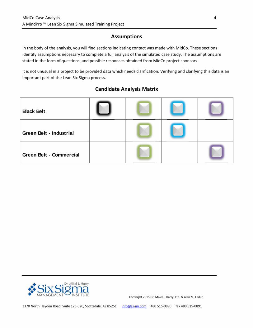
Candidate Analysis Matrix
Black Belt
Green Belt - Industrial
Green Belt - Commercial
MidCo Case Analysis 5
A MindPro ™ Lean Six Sigma Simulated Training Project
Copyright 2015 Dr. Mikel J. Harry, Ltd. & Alan M. Leduc
3370 North Hayden Road, Suite 123‐320, Scottsdale, AZ 85251 info@ss‐mi.com 480 515‐0890 fax 480 515‐0891
Executive Summary
MidCo requested that we analyze data from their Multi‐National 5 location operation. Market share has
been increasing for the past 3 years and they wish to implement a six sigma program on their core operation
with the strategic goal of increased profitability. Tactically they desire to decrease cost and increase
customer satisfaction.
Guiding Questions:
Guiding Questions are those questions that must be answered during the RDMAIC (Recognize‐Design‐
Measure‐Analyze‐Improve‐Control) process of Six Sigma Analysis.
R What business performance metric should be used to drive Six Sigma?
D What product characteristics must be isolated and improved?
M What is the actual and potential capability of the core CTQ’s?
A What is the actual and potential capability of the CTP’s?
I What are the Vital Few CTP’s and what should their optimal settings be?
C What level of process control can be sustained over time?
Recognize
What business performance metric should be used to drive Six Sigma?
Yield in the United States facility was the primary metric that we utilized to drive Six Sigma. We have yet to
do the follow‐up analysis, but since we improved yield we should see the following effects in the follow‐up
analysis: reduced COPQ; increased productivity; more consistency with deliveries; decreased costs;
increased profitability; and improved customer satisfaction. Once the follow‐up analysis validates our gains
we should use the work in the United States plant as a standard for improving the other facilities.
MidCo Case Analysis 6
A MindPro ™ Lean Six Sigma Simulated Training Project Executive Summary
Copyright 2015 Dr. Mikel J. Harry, Ltd. & Alan M. Leduc
3370 North Hayden Road, Suite 123‐320, Scottsdale, AZ 85251 info@ss‐mi.com 480 515‐0890 fax 480 515‐0891
Define
What product characteristics must be isolated and improved?
In the United States facility, we identified four CTQ’s (1,2,3, and 7) that should be considered for isolation
and improvement. However, since this was MidCo’s first Six Sigma project, we were asked to provide
improvement estimates based only the two CTQ’s that had the highest failure rate, CTQ’s 1 and 2.
Measure
What is the actual and potential capability of the core CTQ’s?
The initial analysis of capability is summarized as follows:
CTQ‐1 had short term capability of 3.54 sigma (Cp = 1.18) and a long term capability of 2.22 sigma
(Pp = 0.74). It was evident that the overall capability of the process would be improved by
eliminating assignable causes. CTQ‐1 was also centered below (mean = 73.4) the target (80).
CTQ‐2 had a short term capability of 0.63 sigma (Cp = 0.21) and a long term capability of 0.57 sigma
(Pp = 0.19). Since the Cp and Pp values were comparable there is little room for improvement in
process without improving the technology. CTQ‐2 was centered above the (mean = 534.6) the target
(500).
Analyze
What is the actual and potential capability of the CTP’s?
MidCo Case Analysis 7
A MindPro ™ Lean Six Sigma Simulated Training Project Executive Summary
Copyright 2015 Dr. Mikel J. Harry, Ltd. & Alan M. Leduc
3370 North Hayden Road, Suite 123‐320, Scottsdale, AZ 85251 info@ss‐mi.com 480 515‐0890 fax 480 515‐0891
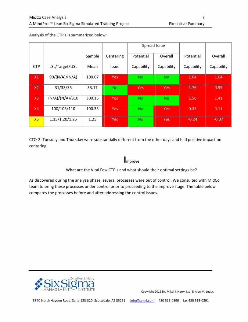
Analysis of the CTP’s is summarized below:
CTP LSL/Target/USL
Sample
Mean
Centering
Issue
Spread Issue
Potential
Capability
Overall
Capability
Potential
Capability
Overall
Capability
X1 90/(N/A)/(N/A) 100.07 Yes No No 1.04 1.04
X2 31/33/35 33.17 No Yes Yes 1.76 0.99
X3 (N/A)/(N/A)/310 300.15 Yes No No 1.56 1.41
X4 100/105/110 100.33 Yes No Yes 0.35 0.11
X5 1.15/1.20/1.25 1.25 Yes No Yes ‐0.24 ‐0.07
CTQ‐2: Tuesday and Thursday were substantially different from the other days and had positive impact on
centering.
Improve
What are the Vital Few CTP’s and what should their optimal settings be?
As discovered during the analyze phase, several processes were out of control. We consulted with MidCo
team to bring these processes under control prior to proceeding to the improve stage. The table below
compares the processes before and after addressing the control issues.
MidCo Case Analysis 8
A MindPro ™ Lean Six Sigma Simulated Training Project Executive Summary
Copyright 2015 Dr. Mikel J. Harry, Ltd. & Alan M. Leduc
3370 North Hayden Road, Suite 123‐320, Scottsdale, AZ 85251 info@ss‐mi.com 480 515‐0890 fax 480 515‐0891
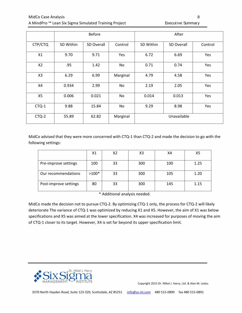
Before After
CTP/CTQ SD Within SD Overall Control SD Within SD Overall Control
X1 9.70 9.71 Yes 6.72 6.69 Yes
X2 .95 1.42 No 0.71 0.74 Yes
X3 6.29 6.99 Marginal 4.79 4.58 Yes
X4 0.934 2.99 No 2.19 2.05 Yes
X5 0.006 0.021 No 0.014 0.013 Yes
CTQ‐1 9.88 15.84 No 9.29 8.98 Yes
CTQ‐2 55.89 62.82 Marginal Unavailable
MidCo advised that they were more concerned with CTQ‐1 than CTQ‐2 and made the decision to go with the
following settings:
X1 X2 X3 X4 X5
Pre‐improve settings 100 33 300 100 1.25
Our recommendations >100* 33 300 105 1.20
Post‐improve settings 80 33 300 145 1.15
* Additional analysis needed.
MidCo made the decision not to pursue CTQ‐2. By optimizing CTQ‐1 only, the process for CTQ‐2 will likely
deteriorate The variance of CTQ‐1 was optimized by reducing X1 and X5. However, the aim of X1 was below
specifications and X5 was aimed at the lower specification. X4 was increased for purposes of moving the aim
of CTQ‐1 closer to its target. However, X4 is set far beyond its upper specification limit.
MidCo Case Analysis 9
A MindPro ™ Lean Six Sigma Simulated Training Project Executive Summary
Copyright 2015 Dr. Mikel J. Harry, Ltd. & Alan M. Leduc
3370 North Hayden Road, Suite 123‐320, Scottsdale, AZ 85251 info@ss‐mi.com 480 515‐0890 fax 480 515‐0891
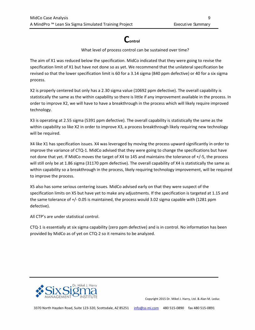
Control
What level of process control can be sustained over time?
The aim of X1 was reduced below the specification. MidCo indicated that they were going to revise the
specification limit of X1 but have not done so as yet. We recommend that the unilateral specification be
revised so that the lower specification limit is 60 for a 3.14 sigma (840 ppm defective) or 40 for a six sigma
process.
X2 is properly centered but only has a 2.30 sigma value (10692 ppm defective). The overall capability is
statistically the same as the within capability so there is little if any improvement available in the process. In
order to improve X2, we will have to have a breakthrough in the process which will likely require improved
technology.
X3 is operating at 2.55 sigma (5391 ppm defective). The overall capability is statistically the same as the
within capability so like X2 in order to improve X3, a process breakthrough likely requiring new technology
will be required.
X4 like X1 has specification issues. X4 was leveraged by moving the process upward significantly in order to
improve the variance of CTQ‐1. MidCo advised that they were going to change the specifications but have
not done that yet. If MidCo moves the target of X4 to 145 and maintains the tolerance of +/‐5, the process
will still only be at 1.86 sigma (31170 ppm defective). The overall capability of X4 is statistically the same as
within capability so a breakthrough in the process, likely requiring technology improvement, will be required
to improve the process.
X5 also has some serious centering issues. MidCo advised early on that they were suspect of the
specification limits on X5 but have yet to make any adjustments. If the specification is targeted at 1.15 and
the same tolerance of +/‐ 0.05 is maintained, the process would 3.02 sigma capable with (1281 ppm
defective).
All CTP’s are under statistical control.
CTQ‐1 is essentially at six sigma capability (zero ppm defective) and is in control. No information has been
provided by MidCo as of yet on CTQ‐2 so it remains to be analyzed.

MidCo Case Analysis 10
A MindPro ™ Lean Six Sigma Simulated Training Project
Copyright 2015 Dr. Mikel J. Harry, Ltd. & Alan M. Leduc
3370 North Hayden Road, Suite 123‐320, Scottsdale, AZ 85251 info@ss‐mi.com 480 515‐0890 fax 480 515‐0891
Additional Tasks
In addition to the six sigma analysis we were ask to analyze a customer survey that was given prior to the six
sigma implementation and a risk analysis calculator.
Survey
Those that have the most need for the MidCo’s product seem to be satisfied with the quality of the product; but,
have a low overall satisfaction with the product. This deserves some investigation.
The Cost and Delivery may be contributors to the overall dissatisfaction but they are not statistically
significant.
A focus group could provide some insight as to other issues that might be degrading overall satisfaction.
Once a list of potential factors is developed in the focus group, a new survey should be done using the
demographics of the group with the most need.
Those with less income tend to be less satisfied with delivery than those with higher income.
This may indicate that those with higher income are using express delivery services that cannot be
afforded by those with less income.
In the survey that is recommended above using the demographics of those with less income, questions
should be ask regarding preferred deliver methods and cost of delivery.
Investigation should be done in Region B with regard to potential delivery issues.
Risk Calculator
The risk calculator provided by MidCo either has an error or the risk factor used in the calculator is misstated.
MidCo stated that the risk factor was the risk of an individual failure exceeding its Limiting Cost. However, the
template is designed so that the risk is actually the risk of the sum of Limiting Costs of all failures of a particular
CTQ exceeding the Monthly Limiting Cost.
MidCo Case Analysis 11
A MindPro ™ Lean Six Sigma Simulated Training Project
Copyright 2015 Dr. Mikel J. Harry, Ltd. & Alan M. Leduc
3370 North Hayden Road, Suite 123‐320, Scottsdale, AZ 85251 info@ss‐mi.com 480 515‐0890 fax 480 515‐0891
Introduction
MidCo Facts:
Product Line: One product line with supporting services
Size: Multi‐National with 5 locations
o South Africa
o Europe
o Pacific Rim
o United States
o Middle East
Market Share: Increasing for the last 3 years
Strategic Goal: Increase profitability
Tactical Goal: Decrease cost and increase customer satisfaction
Operational Focus: Improve yields and decrease defect rates
Operational Target: Improve capability of core process
Operational Plan: Install Six Sigma
MidCo Case Analysis 12
A MindPro ™ Lean Six Sigma Simulated Training Project
Copyright 2015 Dr. Mikel J. Harry, Ltd. & Alan M. Leduc
3370 North Hayden Road, Suite 123‐320, Scottsdale, AZ 85251 info@ss‐mi.com 480 515‐0890 fax 480 515‐0891
Guiding Questions
Guiding Questions are those questions that must be answered during the RDMAIC (Recognize‐Design‐
Measure‐Analyze‐Improve‐Control) process of Six Sigma Analysis.
R What business performance metric should be used to drive Six Sigma?
D What product characteristics must be isolated and improved?
M What is the actual and potential capability of the core CTQ’s?
A What is the actual and potential capability of the CTP’s?
I What are the Vital Few CTP’s and what should their optimal settings be?
C What level of process control can be sustained over time?
MidCo Case Analysis 13
A MindPro ™ Lean Six Sigma Simulated Training Project
Copyright 2015 Dr. Mikel J. Harry, Ltd. & Alan M. Leduc
3370 North Hayden Road, Suite 123‐320, Scottsdale, AZ 85251 info@ss‐mi.com 480 515‐0890 fax 480 515‐0891
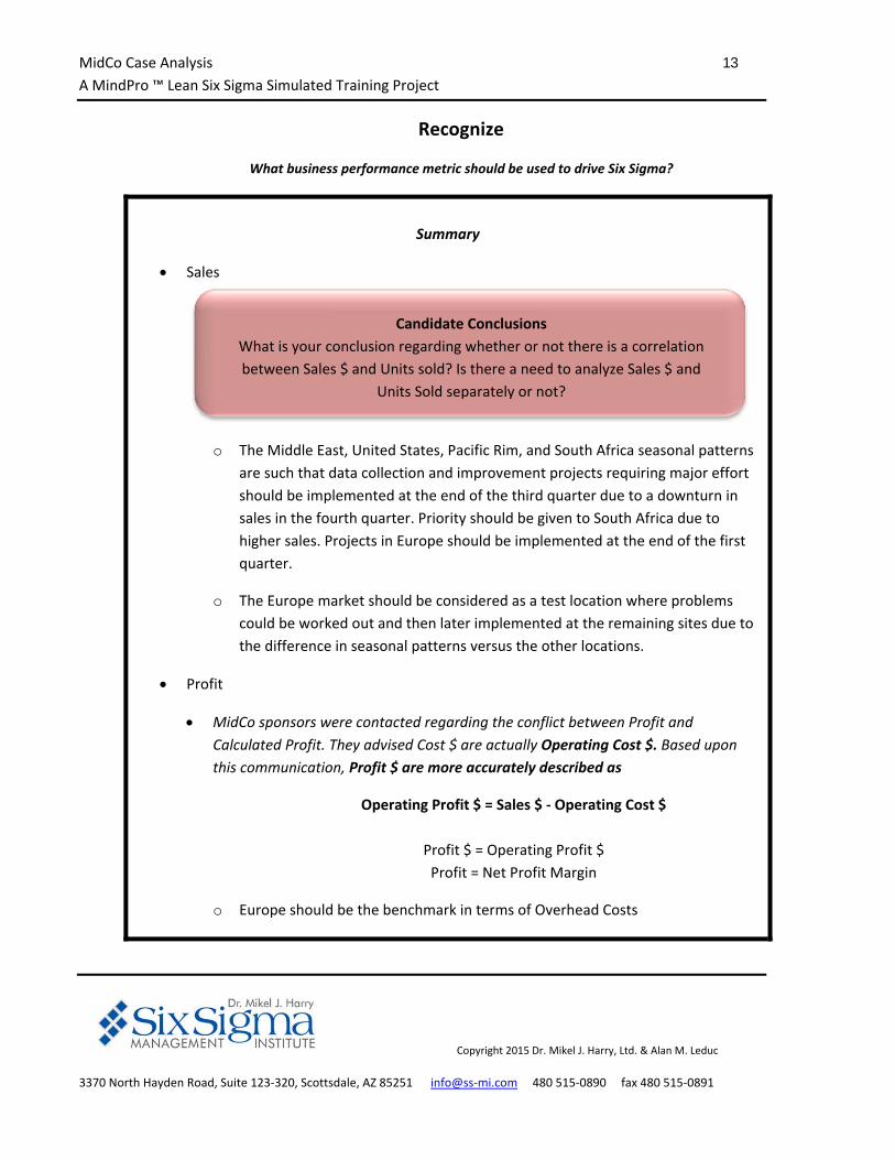
Recognize
What business performance metric should be used to drive Six Sigma?
Summary
Sales
o The Middle East, United States, Pacific Rim, and South Africa seasonal patterns
are such that data collection and improvement projects requiring major effort
should be implemented at the end of the third quarter due to a downturn in
sales in the fourth quarter. Priority should be given to South Africa due to
higher sales. Projects in Europe should be implemented at the end of the first
quarter.
o The Europe market should be considered as a test location where problems
could be worked out and then later implemented at the remaining sites due to
the difference in seasonal patterns versus the other locations.
Profit
MidCo sponsors were contacted regarding the conflict between Profit and
Calculated Profit. They advised Cost $ are actually Operating Cost $. Based upon
this communication, Profit $ are more accurately described as
Operating Profit $ = Sales $ ‐ Operating Cost $
Profit $ = Operating Profit $
Profit = Net Profit Margin
o Europe should be the benchmark in terms of Overhead Costs
Candidate Conclusions
What is your conclusion regarding whether or not there is a correlation
between Sales $ and Units sold? Is there a need to analyze Sales $ and
Units Sold separately or not?
MidCo Case Analysis 14
A MindPro ™ Lean Six Sigma Simulated Training Project Recognize
Copyright 2015 Dr. Mikel J. Harry, Ltd. & Alan M. Leduc
3370 North Hayden Road, Suite 123‐320, Scottsdale, AZ 85251 info@ss‐mi.com 480 515‐0890 fax 480 515‐0891
o The Middle East appears to be the most balanced location in terms of Profit
Analysis and has the second highest Net Profit Margin at 7.76%.
o The Pacific Rim, Europe, and the Middle East have reasonable Net Profit
Margins and an adequate overhead structure.
o Overhead Costs should be evaluated in the South Africa facility.
o The Middle East, South Africa, and Pacific Rim facilities all have Operating
Profits as a percent of total that outpace their sales as a percent of total. We
should look to these locations for benchmarking the operation side of our
facilities.
o The United States facility appears to need the most attention.
o There is a correlation between Sales and Operating Profit. This may mean that
we have utilization issues in some of the facilities.
COPQ
o Although Cost of Poor Quality is generally difficult to measure, it appears that
MidCo is being consistent in the way that it measures COPQ given the relative
stability in the Europe, Pacific Rim, and Middle East facilities which are hovering
around 5% of Sales regardless of sales levels.
o We need to investigate Quality Issues in both South Africa and the United
States.
o There is an inverse correlation between yield and COPQ, as yield increases,
COPQ decreases.
Candidate Conclusions
What are revenues, operating profit, net profit, and profit margin for the
United States location?
MidCo Case Analysis 15
A MindPro ™ Lean Six Sigma Simulated Training Project Recognize
Copyright 2015 Dr. Mikel J. Harry, Ltd. & Alan M. Leduc
3370 North Hayden Road, Suite 123‐320, Scottsdale, AZ 85251 info@ss‐mi.com 480 515‐0890 fax 480 515‐0891
Yield
o The United States has by far the most significant variation and should be the
focus of yield analysis.
o Yield has a positive correlation to Net Profit Margin; but not to Operating Profit.
Cost
o There is no indication of a difference in the variances or means of Cost$ in the
first half of the year versus the last half of the year.
While in the long term we might want to look at the overheard structure of South Africa, we do
not currently have sufficient data to do this analysis.
As we proceed to the Design Stage the focus should be on Yield as the primary metric to drive
Six Sigma. Analysis has shown that as yield is improved, COPQ will be reduced resulting in an
increase in productivity and Net Profit Margin. More consistency in deliveries should be
attained. Focusing on yield should allow achievement of the strategic objective of “Increasing
profitability” and accomplish the tactical objectives of “decreasing costs and increasing
customer satisfaction.
The yield of the United States facility had a significant negative impact on the overall yield of
the corporation and thus should be the focus of our analysis in the Design Stage.
Candidate Conclusions
Is there a difference in the variances of means of Cost $ in the first half of
the year versus the last half of the year?
MidCo Case Analysis 16
A MindPro ™ Lean Six Sigma Simulated Training Project Recognize
Copyright 2015 Dr. Mikel J. Harry, Ltd. & Alan M. Leduc
3370 North Hayden Road, Suite 123‐320, Scottsdale, AZ 85251 info@ss‐mi.com 480 515‐0890 fax 480 515‐0891
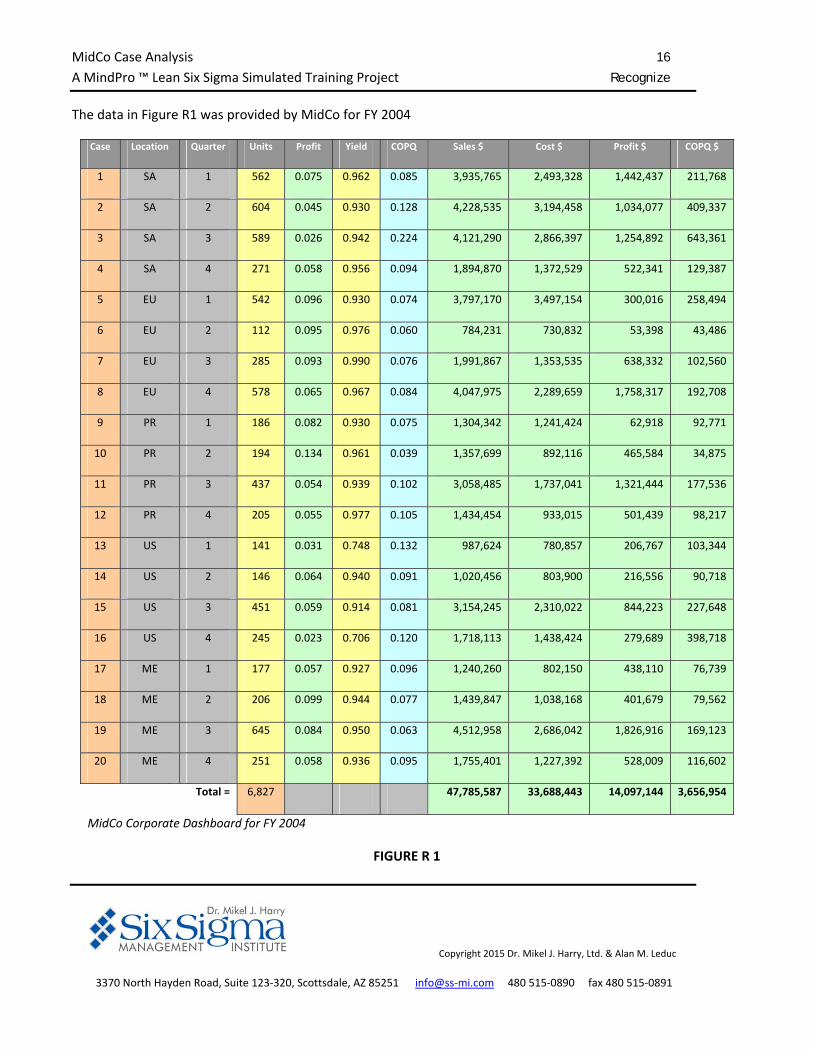
The data in Figure R1 was provided by MidCo for FY 2004
Case Location Quarter Units Profit Yield COPQ Sales $ Cost $ Profit $ COPQ $
1 SA 1 562 0.075 0.962 0.085 3,935,765 2,493,328 1,442,437 211,768
2 SA 2 604 0.045 0.930 0.128 4,228,535 3,194,458 1,034,077 409,337
3 SA 3 589 0.026 0.942 0.224 4,121,290 2,866,397 1,254,892 643,361
4 SA 4 271 0.058 0.956 0.094 1,894,870 1,372,529 522,341 129,387
5 EU 1 542 0.096 0.930 0.074 3,797,170 3,497,154 300,016 258,494
6 EU 2 112 0.095 0.976 0.060 784,231 730,832 53,398 43,486
7 EU 3 285 0.093 0.990 0.076 1,991,867 1,353,535 638,332 102,560
8 EU 4 578 0.065 0.967 0.084 4,047,975 2,289,659 1,758,317 192,708
9 PR 1 186 0.082 0.930 0.075 1,304,342 1,241,424 62,918 92,771
10 PR 2 194 0.134 0.961 0.039 1,357,699 892,116 465,584 34,875
11 PR 3 437 0.054 0.939 0.102 3,058,485 1,737,041 1,321,444 177,536
12 PR 4 205 0.055 0.977 0.105 1,434,454 933,015 501,439 98,217
13 US 1 141 0.031 0.748 0.132 987,624 780,857 206,767 103,344
14 US 2 146 0.064 0.940 0.091 1,020,456 803,900 216,556 90,718
15 US 3 451 0.059 0.914 0.081 3,154,245 2,310,022 844,223 227,648
16 US 4 245 0.023 0.706 0.120 1,718,113 1,438,424 279,689 398,718
17 ME 1 177 0.057 0.927 0.096 1,240,260 802,150 438,110 76,739
18 ME 2 206 0.099 0.944 0.077 1,439,847 1,038,168 401,679 79,562
19 ME 3 645 0.084 0.950 0.063 4,512,958 2,686,042 1,826,916 169,123
20 ME 4 251 0.058 0.936 0.095 1,755,401 1,227,392 528,009 116,602
Total = 6,827 47,785,587 33,688,443 14,097,144 3,656,954
MidCo Corporate Dashboard for FY 2004
FIGURE R 1
MidCo Case Analysis 17
A MindPro ™ Lean Six Sigma Simulated Training Project Recognize
Copyright 2015 Dr. Mikel J. Harry, Ltd. & Alan M. Leduc
3370 North Hayden Road, Suite 123‐320, Scottsdale, AZ 85251 info@ss‐mi.com 480 515‐0890 fax 480 515‐0891
The next several pages provide a thorough analysis of the variables provided in the data from MidCo. The
purpose of the analysis is to determine which of the performance variables should be used to drive Six Sigma.
The Recognize Phase analysis was dissected in to analysis of five sections:
1. Sales Analysis
2. Profit (Operating Profit and Net Profit Margin)
3. Cost of Poor Quality
4. Yield
5. Cost
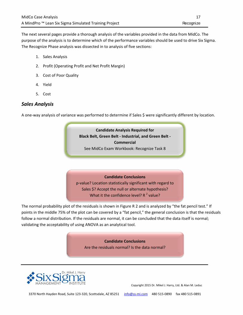
Sales Analysis
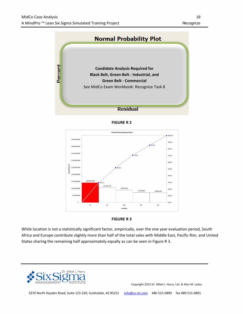
A one‐way analysis of variance was performed to determine if Sales $ were significantly different by location.
The normal probability plot of the residuals is shown in Figure R 2 and is analyzed by “the fat pencil test.” If
points in the middle 75% of the plot can be covered by a “fat pencil,” the general conclusion is that the residuals
follow a normal distribution. If the residuals are normal, it can be concluded that the data itself is normal;
validating the acceptability of using ANOVA as an analytical tool.
Candidate Analysis Required for
Black Belt, Green Belt ‐ Industrial, and Green Belt ‐
Commercial
See MidCo Exam Workbook: Recognize Task 8
Candidate Conclusions
p‐value? Location statistically significant with regard to
Sales $? Accept the null or alternate hypothesis?
What it the confidence level? R 2 value?
Candidate Conclusions
Are the residuals normal? Is the data normal?
MidCo Case Analysis 18
A MindPro ™ Lean Six Sigma Simulated Training Project Recognize
Copyright 2015 Dr. Mikel J. Harry, Ltd. & Alan M. Leduc
3370 North Hayden Road, Suite 123‐320, Scottsdale, AZ 85251 info@ss‐mi.com 480 515‐0890 fax 480 515‐0891
FIGURE R 2
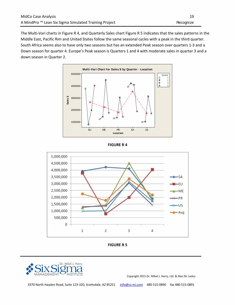
FIGURE R 3
While location is not a statistically significant factor, empirically, over the one year evaluation period, South
Africa and Europe contribute slightly more than half of the total sales with Middle East, Pacific Rim, and United
States sharing the remaining half approximately equally as can be seen in Figure R 3.
Candidate Analysis Required for
Black Belt, Green Belt ‐ Industrial, and
Green Belt ‐ Commercial
See MidCo Exam Workbook: Recognize Task 8
MidCo Case Analysis 19
A MindPro ™ Lean Six Sigma Simulated Training Project Recognize
Copyright 2015 Dr. Mikel J. Harry, Ltd. & Alan M. Leduc
3370 North Hayden Road, Suite 123‐320, Scottsdale, AZ 85251 info@ss‐mi.com 480 515‐0890 fax 480 515‐0891
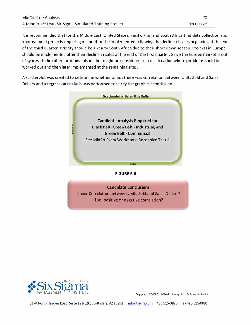
The Multi‐Vari charts in Figure R 4, and Quarterly Sales chart Figure R 5 indicates that the sales patterns in the
Middle East, Pacific Rim and United States follow the same seasonal cycles with a peak in the third quarter.
South Africa seems also to have only two seasons but has an extended Peak season over quarters 1‐3 and a
Down season for quarter 4. Europe’s Peak season is Quarters 1 and 4 with moderate sales in quarter 3 and a
down season in Quarter 2.
Location
Sale
s $
USSAPRMEEU
5000000
4000000
3000000
2000000
1000000
Quarter1234
Multi-Vari Chart for Sales $ by Quarter - Location
FIGURE R 4
FIGURE R 5
MidCo Case Analysis 20
A MindPro ™ Lean Six Sigma Simulated Training Project Recognize
Copyright 2015 Dr. Mikel J. Harry, Ltd. & Alan M. Leduc
3370 North Hayden Road, Suite 123‐320, Scottsdale, AZ 85251 info@ss‐mi.com 480 515‐0890 fax 480 515‐0891
It is recommended that for the Middle East, United States, Pacific Rim, and South Africa that data collection and
improvement projects requiring major effort be implemented following the decline of sales beginning at the end
of the third quarter. Priority should be given to South Africa due to their short down season. Projects in Europe
should be implemented after their decline in sales at the end of the first quarter. Since the Europe market is out
of sync with the other locations this market might be considered as a test location where problems could be
worked out and then later implemented at the remaining sites.
A scatterplot was created to determine whether or not there was correlation between Units Sold and Sales
Dollars and a regression analysis was performed to verify the graphical conclusion.
FIGURE R 6
Candidate Analysis Required for
Black Belt, Green Belt ‐ Industrial, and
Green Belt ‐ Commercial
See MidCo Exam Workbook: Recognize Task 4
Candidate Conclusions
Linear Correlation between Units Sold and Sales Dollars?
If so, positive or negative correlation?
MidCo Case Analysis 21
A MindPro ™ Lean Six Sigma Simulated Training Project Recognize
Copyright 2015 Dr. Mikel J. Harry, Ltd. & Alan M. Leduc
3370 North Hayden Road, Suite 123‐320, Scottsdale, AZ 85251 info@ss‐mi.com 480 515‐0890 fax 480 515‐0891
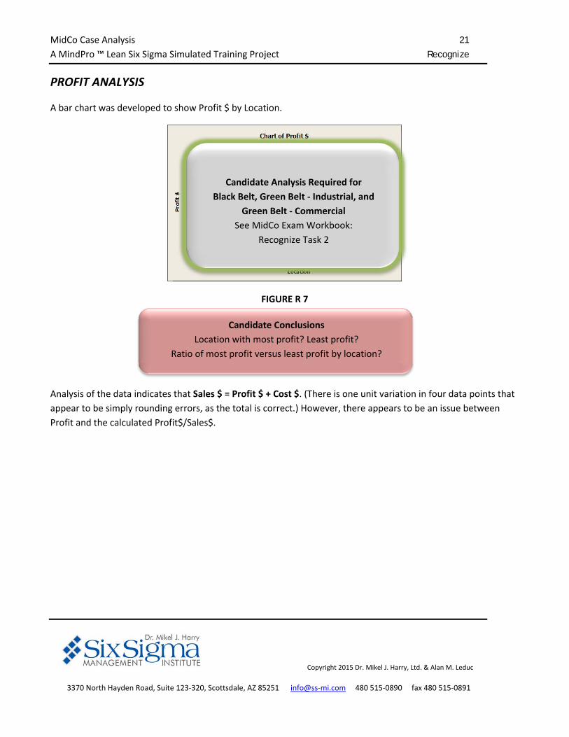
PROFIT ANALYSIS
A bar chart was developed to show Profit $ by Location.
MEUSPREUSA
4000000
3000000
2000000
1000000
0
Location
Prof
it $
Chart of Profit $
FIGURE R 7
Analysis of the data indicates that Sales $ = Profit $ + Cost $. (There is one unit variation in four data points that
appear to be simply rounding errors, as the total is correct.) However, there appears to be an issue between
Profit and the calculated Profit$/Sales$.
Candidate Analysis Required for
Black Belt, Green Belt ‐ Industrial, and
Green Belt ‐ Commercial
See MidCo Exam Workbook:
Recognize Task 2
Candidate Conclusions
Location with most profit? Least profit?
Ratio of most profit versus least profit by location?
MidCo Case Analysis 22
A MindPro ™ Lean Six Sigma Simulated Training Project Recognize
Copyright 2015 Dr. Mikel J. Harry, Ltd. & Alan M. Leduc
3370 North Hayden Road, Suite 123‐320, Scottsdale, AZ 85251 info@ss‐mi.com 480 515‐0890 fax 480 515‐0891
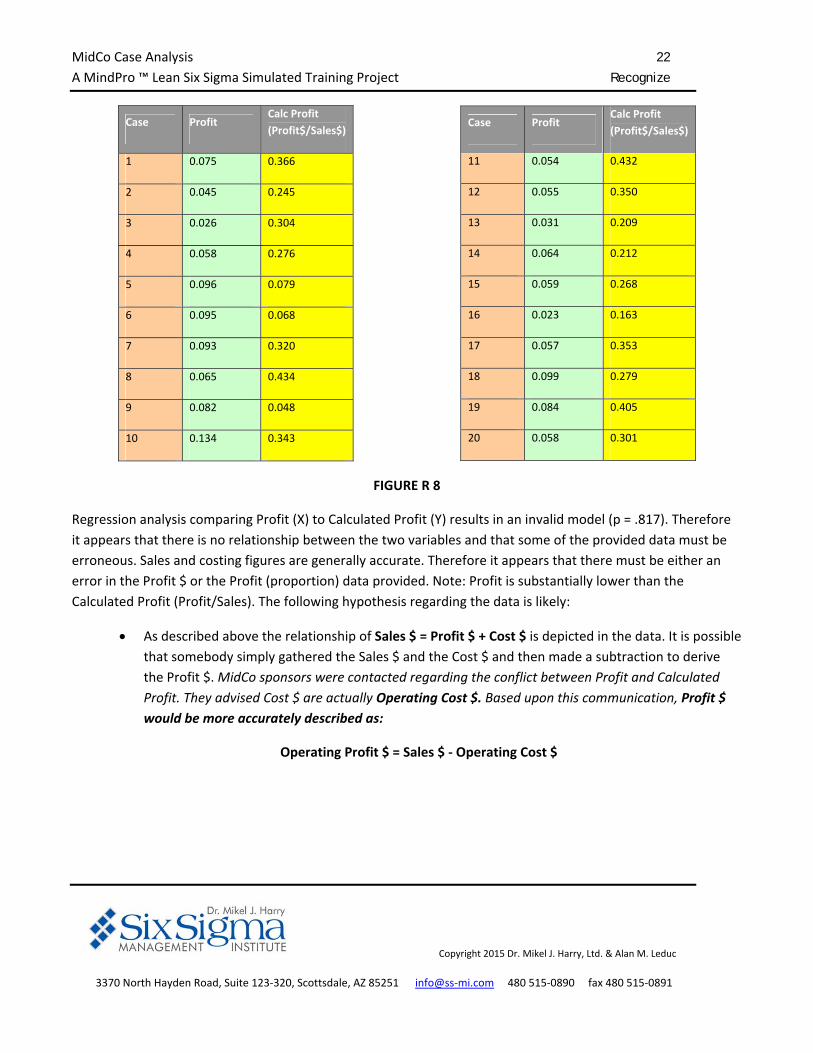
Case Profit Calc Profit
(Profit$/Sales$)
1 0.075 0.366
2 0.045 0.245
3 0.026 0.304
4 0.058 0.276
5 0.096 0.079
6 0.095 0.068
7 0.093 0.320
8 0.065 0.434
9 0.082 0.048
10 0.134 0.343
Case Profit Calc Profit
(Profit$/Sales$)
11 0.054 0.432
12 0.055 0.350
13 0.031 0.209
14 0.064 0.212
15 0.059 0.268
16 0.023 0.163
17 0.057 0.353
18 0.099 0.279
19 0.084 0.405
20 0.058 0.301
FIGURE R 8
Regression analysis comparing Profit (X) to Calculated Profit (Y) results in an invalid model (p = .817). Therefore
it appears that there is no relationship between the two variables and that some of the provided data must be
erroneous. Sales and costing figures are generally accurate. Therefore it appears that there must be either an
error in the Profit $ or the Profit (proportion) data provided. Note: Profit is substantially lower than the
Calculated Profit (Profit/Sales). The following hypothesis regarding the data is likely:
As described above the relationship of Sales $ = Profit $ + Cost $ is depicted in the data. It is possible
that somebody simply gathered the Sales $ and the Cost $ and then made a subtraction to derive
the Profit $. MidCo sponsors were contacted regarding the conflict between Profit and Calculated
Profit. They advised Cost $ are actually Operating Cost $. Based upon this communication, Profit $
would be more accurately described as:
Operating Profit $ = Sales $ ‐ Operating Cost $
MidCo Case Analysis 23
A MindPro ™ Lean Six Sigma Simulated Training Project Recognize
Copyright 2015 Dr. Mikel J. Harry, Ltd. & Alan M. Leduc
3370 North Hayden Road, Suite 123‐320, Scottsdale, AZ 85251 info@ss‐mi.com 480 515‐0890 fax 480 515‐0891
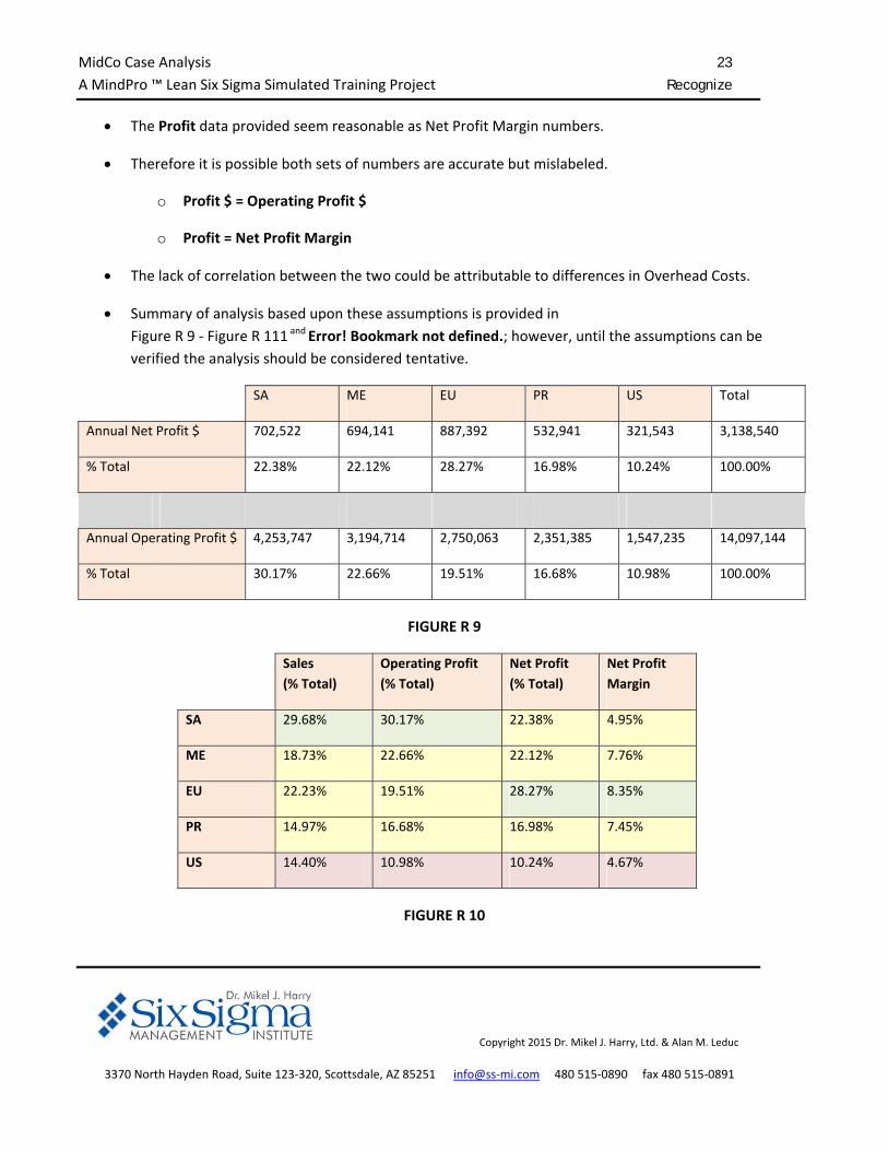
The Profit data provided seem reasonable as Net Profit Margin numbers.
Therefore it is possible both sets of numbers are accurate but mislabeled.
o Profit $ = Operating Profit $
o Profit = Net Profit Margin
The lack of correlation between the two could be attributable to differences in Overhead Costs.
Summary of analysis based upon these assumptions is provided in
Figure R 9 ‐ Figure R 111 and Error! Bookmark not defined.; however, until the assumptions can be
verified the analysis should be considered tentative.
SA ME EU PR US Total
Annual Net Profit $ 702,522 694,141 887,392 532,941 321,543 3,138,540
% Total 22.38% 22.12% 28.27% 16.98% 10.24% 100.00%
Annual Operating Profit $ 4,253,747 3,194,714 2,750,063 2,351,385 1,547,235 14,097,144
% Total 30.17% 22.66% 19.51% 16.68% 10.98% 100.00%
FIGURE R 9
Sales
(% Total)
Operating Profit
(% Total)
Net Profit
(% Total)
Net Profit
Margin
SA 29.68% 30.17% 22.38% 4.95%
ME 18.73% 22.66% 22.12% 7.76%
EU 22.23% 19.51% 28.27% 8.35%
PR 14.97% 16.68% 16.98% 7.45%
US 14.40% 10.98% 10.24% 4.67%
FIGURE R 10
MidCo Case Analysis 24
A MindPro ™ Lean Six Sigma Simulated Training Project Recognize
Copyright 2015 Dr. Mikel J. Harry, Ltd. & Alan M. Leduc
3370 North Hayden Road, Suite 123‐320, Scottsdale, AZ 85251 info@ss‐mi.com 480 515‐0890 fax 480 515‐0891
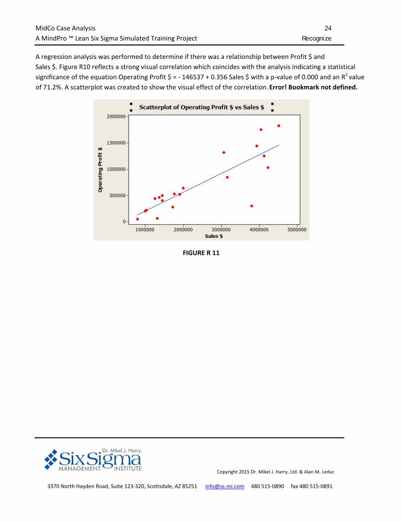
A regression analysis was performed to determine if there was a relationship between Profit $ and
Sales $. Figure R10 reflects a strong visual correlation which coincides with the analysis indicating a statistical
significance of the equation Operating Profit $ = ‐ 146537 + 0.356 Sales $ with a p‐value of 0.000 and an R2 value
of 71.2%. A scatterplot was created to show the visual effect of the correlation. Error! Bookmark not defined.
FIGURE R 11
MidCo Case Analysis 25
A MindPro ™ Lean Six Sigma Simulated Training Project Recognize
Copyright 2015 Dr. Mikel J. Harry, Ltd. & Alan M. Leduc
3370 North Hayden Road, Suite 123‐320, Scottsdale, AZ 85251 info@ss‐mi.com 480 515‐0890 fax 480 515‐0891
A regression analysis was done to determine if there is a correlation between Profit$ and the COPQ$.
7000006000005000004000003000002000001000000
2000000
1500000
1000000
500000
0
COPQ $
Prof
it $
Scatterplot of Profit $ vs COPQ $
FIGURE R 12
A request was made by MidCo to determine how the variation in Profit $ compared from location to location
versus Quarter to Quarter. The recommended tool was the multi‐vari chart ‐ provided in
Figure R 13. The chart on the left shows the location mean in red and the quarters plotted in each grouping. The
chart on the right shows the quarterly mean in red and has locations plotted in each grouping. It is difficult to
determine from these charts, whether location to location or quarter to quarter has the most variation. Multi‐
vari charts are excellent for showing patterns; calculation and comparison of standard deviation or ANOVA are
better tools for comparing variation.
Candidate Analysis Required for
Black Belt, Green Belt ‐ Industrial, and
Green Belt ‐ Commercial
See MidCo Exam Workbook: Recognize Task 5
Candidate Conclusions
Linear Correlation between Profit $ and COPQ $?
If so, positive or negative correlation?
MidCo Case Analysis 26
A MindPro ™ Lean Six Sigma Simulated Training Project Recognize
Copyright 2015 Dr. Mikel J. Harry, Ltd. & Alan M. Leduc
3370 North Hayden Road, Suite 123‐320, Scottsdale, AZ 85251 info@ss‐mi.com 480 515‐0890 fax 480 515‐0891
USSAPRMEEU
2000000
1500000
1000000
500000
0
Location
Prof
it $
1234
Quarter
Multi-Vari Chart for Profit $ by Quarter - Location
4321
2000000
1500000
1000000
500000
0
Quarter
Prof
it $
EUMEPRSAUS
Location
Multi-Vari Chart for Profit $ by Location - Quarter
FIGURE R 13
Since it is not clear from the multi‐vari charts whether location to location or quarter to quarter has the most
variation, a statistical analysis was performed to determine the standard deviation.
Location Profit $ Quarter Profit $
SA 4,253,747 1 2,450,248
EU 2,750,063 2 2,171,294
PR 2,351,385 3 5,885,807
US 1,547,235 4 3,589,795
ME 3,194,714
Standard Deviation = Standard Deviation =
FIGURE R 14
An analysis of variance was also performed analyzing with location and quarters as the factors and Profit $ as
the response.
Candidate Analysis Required for
Black Belt, Green Belt ‐ Industrial, and
Green Belt ‐ Commercial
See MidCo Exam Workbook:
Recognize Task 6
Candidate Analysis Required for
Black Belt, Green Belt ‐ Industrial, and
Green Belt ‐ Commercial
See MidCo Exam Workbook:
Recognize Task 6
Candidate Analysis Required for
Black Belt, Green Belt ‐ Industrial, and Green Belt ‐ Commercial
See MidCo Exam Workbook:
Recognize Task 6
Candidate Conclusions
Considering Location‐to‐Location versus Quarter‐to‐
Quarter, where does the most variation in Profit $ occur?
MidCo Case Analysis 27
A MindPro ™ Lean Six Sigma Simulated Training Project Recognize
Copyright 2015 Dr. Mikel J. Harry, Ltd. & Alan M. Leduc
3370 North Hayden Road, Suite 123‐320, Scottsdale, AZ 85251 info@ss‐mi.com 480 515‐0890 fax 480 515‐0891
Casual Observations with regard to Profit Analysis:
South Africa accounts for nearly one‐third of the Sales and Total Operating Profit for the corporation but
only about one‐fifth of the Net Profit. South Africa is near the bottom in terms of Net Profit Margin at 4.95%.
The United States is at the bottom with 4.67% and Europe is at the top with 8.35%.
o Overhead Costs should be evaluated in the South Africa facility.
Europe accounts for slightly more than one‐fifth of corporate Sales and slightly less than one‐fifth of the
Total Operating Profit; however, Europe accounts for slightly more than one‐fourth of the Net Profit and is
the Net Profit Margin leader at 8.35%.
o It appears the Europe should be the benchmark in terms of Overhead Costs.
The Middle East accounts for about one‐sixth of corporate Sales and more than one‐fifth of the Total
Operating Profit and Net Profit. The Middle East has the second highest Net Profit Margin at 7.76%.
o The Middle East appears to be the most balanced location in terms of Profit Analysis.
The Pacific Rim like the United States only accounts for about one‐seventh of corporate Sales; but, unlike
the United States, accounts for approximately one‐sixth of the Total Operating Profit and Net Profit. The
Pacific Rim has a Net Profit Margin of 7.45% which compares favorably with Europe and the Middle East.
o The Pacific Rim appears favorable when evaluating the overall profit picture.
The United States accounts for about one‐seventh of corporate Sales. However, Operating Profit and Net
Profit are only about one‐tenth of the corporation’s total. The Net Profit Margin is the lowest of all facilities
at 4.67%.
o The United States facility is substantially below the other facilities in terms of profit analysis.
MidCo Case Analysis 28
A MindPro ™ Lean Six Sigma Simulated Training Project Recognize
Copyright 2015 Dr. Mikel J. Harry, Ltd. & Alan M. Leduc
3370 North Hayden Road, Suite 123‐320, Scottsdale, AZ 85251 info@ss‐mi.com 480 515‐0890 fax 480 515‐0891
General Conclusions from Profit Analysis:
The overhead structure for South Africa should be evaluated.
o This is the leading facility in terms of Revenue and Operating Profit. If the overhead structure
can be improved this facility could be the benchmark facility.
o We should look at Europe as the Benchmark facility for evaluating the South Africa overhead
structure.
The Pacific Rim, Europe, and the United States appear to have an adequate overhead structure.
However, their overhead structures should be compared to Europe in order to gain marginal
improvements.
The Middle East, South Africa, and Pacific Rim facilities all have Operating Profits as a percent of total
which outpace their sales as a percent of total. These locations should be utilized for benchmarking the
operation side the facilities.
The Middle East and Pacific Rim facilities appear to in good operational and fiscal condition.
The United States facility appears to need the most attention.
o It has the lowest revenues at 14.40% of .total
o It has the lowest operating profit at 10.98% of total.
o It has the lowest net profit at 10.24% of total
o It has the lowest net profit margin at 4.67%
Regression analysis reveals that there is a correlation between Sales and Operating Profit. The
regression equation is Operating Profit $ = ‐0.147 + 0.356 Sales $. R2 = .712, that is 71.2% of the variation
in Profit is explained by Sales $’s which for cross‐sectional data is excellent.
o This may mean there are utilization issues in some of the facilities.
MidCo Case Analysis 29
A MindPro ™ Lean Six Sigma Simulated Training Project Recognize
Copyright 2015 Dr. Mikel J. Harry, Ltd. & Alan M. Leduc
3370 North Hayden Road, Suite 123‐320, Scottsdale, AZ 85251 info@ss‐mi.com 480 515‐0890 fax 480 515‐0891
Analysis of Cost of Poor Quality (COPQ)
MidCo personnel were interested in determining whether or not COPQ$ was higher in any particular quarter. A
bar Chart was developed from the reported data and is displayed in Figure R 15.
4321
1400000
1200000
1000000
800000
600000
400000
200000
0
Quarter
COPQ
$Chart of COPQ $
FIGURE R 15
FIGURE R 16
Candidate Analysis Required for
Black Belt, Green Belt ‐ Industrial, and
Green Belt ‐ Commercial
See MidCo Exam Workbook:
Recognize Task 1
Candidate Conclusions
In which Quarter did the highest COPQ $ occur?
Candidate Analysis Required for
Black Belt, Green Belt ‐ Industrial, and
Green Belt ‐ Commercial
See MidCo Exam Workbook:
Recognize Task 3
MidCo Case Analysis 30
A MindPro ™ Lean Six Sigma Simulated Training Project Recognize
Copyright 2015 Dr. Mikel J. Harry, Ltd. & Alan M. Leduc
3370 North Hayden Road, Suite 123‐320, Scottsdale, AZ 85251 info@ss‐mi.com 480 515‐0890 fax 480 515‐0891
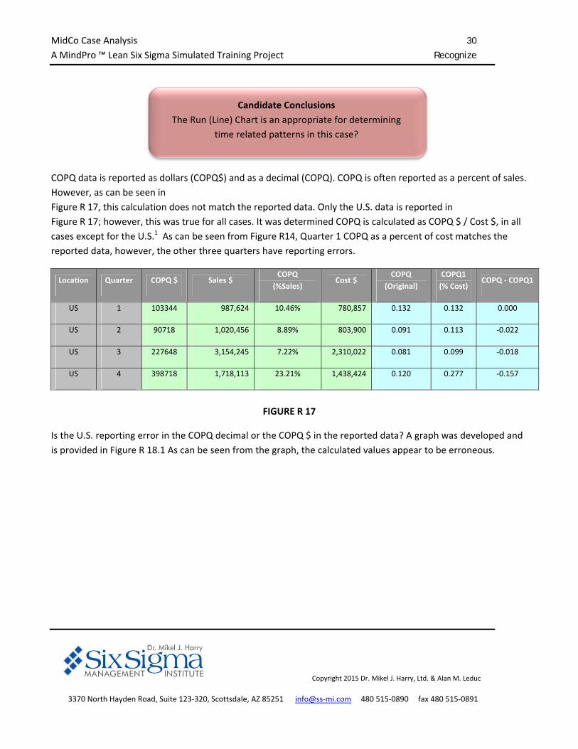
COPQ data is reported as dollars (COPQ$) and as a decimal (COPQ). COPQ is often reported as a percent of sales.
However, as can be seen in
Figure R 17, this calculation does not match the reported data. Only the U.S. data is reported in
Figure R 17; however, this was true for all cases. It was determined COPQ is calculated as COPQ $ / Cost $, in all
cases except for the U.S.1 As can be seen from Figure R14, Quarter 1 COPQ as a percent of cost matches the
reported data, however, the other three quarters have reporting errors.
Location Quarter COPQ $ Sales $ COPQ
(%Sales) Cost $
COPQ
(Original)
COPQ1
(% Cost) COPQ ‐ COPQ1
US 1 103344 987,624 10.46% 780,857 0.132 0.132 0.000
US 2 90718 1,020,456 8.89% 803,900 0.091 0.113 ‐0.022
US 3 227648 3,154,245 7.22% 2,310,022 0.081 0.099 ‐0.018
US 4 398718 1,718,113 23.21% 1,438,424 0.120 0.277 ‐0.157
FIGURE R 17
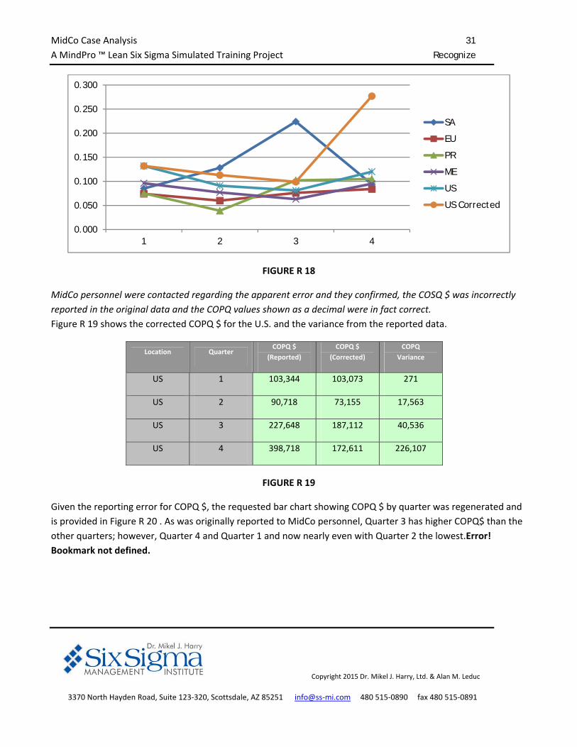
Is the U.S. reporting error in the COPQ decimal or the COPQ $ in the reported data? A graph was developed and
is provided in Figure R 18.1 As can be seen from the graph, the calculated values appear to be erroneous.
Candidate Conclusions
The Run (Line) Chart is an appropriate for determining
time related patterns in this case?
MidCo Case Analysis 31
A MindPro ™ Lean Six Sigma Simulated Training Project Recognize
Copyright 2015 Dr. Mikel J. Harry, Ltd. & Alan M. Leduc
3370 North Hayden Road, Suite 123‐320, Scottsdale, AZ 85251 info@ss‐mi.com 480 515‐0890 fax 480 515‐0891
FIGURE R 18
MidCo personnel were contacted regarding the apparent error and they confirmed, the COSQ $ was incorrectly
reported in the original data and the COPQ values shown as a decimal were in fact correct.
Figure R 19 shows the corrected COPQ $ for the U.S. and the variance from the reported data.
Location Quarter COPQ $
(Reported)
COPQ $
(Corrected)
COPQ
Variance
US 1 103,344 103,073 271
US 2 90,718 73,155 17,563
US 3 227,648 187,112 40,536
US 4 398,718 172,611 226,107
FIGURE R 19
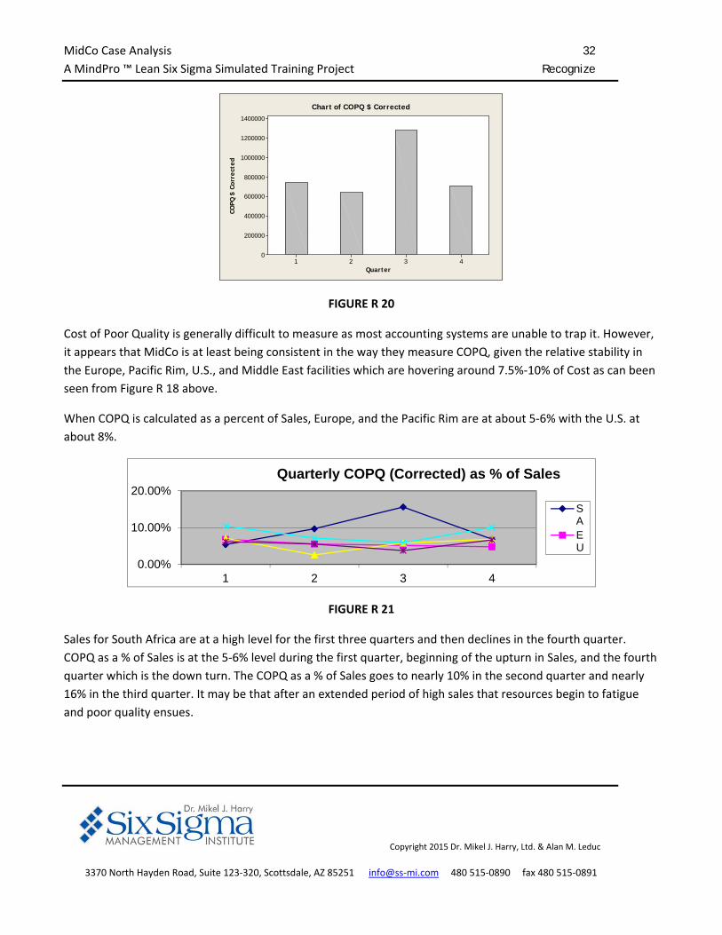
Given the reporting error for COPQ $, the requested bar chart showing COPQ $ by quarter was regenerated and
is provided in Figure R 20 . As was originally reported to MidCo personnel, Quarter 3 has higher COPQ$ than the
other quarters; however, Quarter 4 and Quarter 1 and now nearly even with Quarter 2 the lowest.Error!
Bookmark not defined.
0.000
0.050
0.100
0.150
0.200
0.250
0.300
1 2 3 4
SA
EU
PR
ME
US
US Corrected
MidCo Case Analysis 32
A MindPro ™ Lean Six Sigma Simulated Training Project Recognize
Copyright 2015 Dr. Mikel J. Harry, Ltd. & Alan M. Leduc
3370 North Hayden Road, Suite 123‐320, Scottsdale, AZ 85251 info@ss‐mi.com 480 515‐0890 fax 480 515‐0891
4321
1400000
1200000
1000000
800000
600000
400000
200000
0
Quarter
COPQ
$ C
orre
cted
Chart of COPQ $ Corrected
FIGURE R 20
Cost of Poor Quality is generally difficult to measure as most accounting systems are unable to trap it. However,
it appears that MidCo is at least being consistent in the way they measure COPQ, given the relative stability in
the Europe, Pacific Rim, U.S., and Middle East facilities which are hovering around 7.5%‐10% of Cost as can been
seen from Figure R 18 above.
When COPQ is calculated as a percent of Sales, Europe, and the Pacific Rim are at about 5‐6% with the U.S. at
about 8%.
FIGURE R 21
Sales for South Africa are at a high level for the first three quarters and then declines in the fourth quarter.
COPQ as a % of Sales is at the 5‐6% level during the first quarter, beginning of the upturn in Sales, and the fourth
quarter which is the down turn. The COPQ as a % of Sales goes to nearly 10% in the second quarter and nearly
16% in the third quarter. It may be that after an extended period of high sales that resources begin to fatigue
and poor quality ensues.
0.00%
10.00%
20.00%
1 2 3 4
Quarterly COPQ (Corrected) as % of Sales
SAEU
MidCo Case Analysis 33
A MindPro ™ Lean Six Sigma Simulated Training Project Recognize
Copyright 2015 Dr. Mikel J. Harry, Ltd. & Alan M. Leduc
3370 North Hayden Road, Suite 123‐320, Scottsdale, AZ 85251 info@ss‐mi.com 480 515‐0890 fax 480 515‐0891
The COPQ as % of Sales for the United State is 10.44%, 7.17% and 5.93% for the first three quarters
respectively. The first and second quarters have stable sales and the third quarter is during the peak season. It is
interesting that COPQ improves as sales increases. In the fourth quarter, sales begin to decline and the COPQ
rises to 10.05%. It is a quite peculiar pattern to have much lower COPQ during the high sales periods as
compared to the low sales periods. This should be investigated.
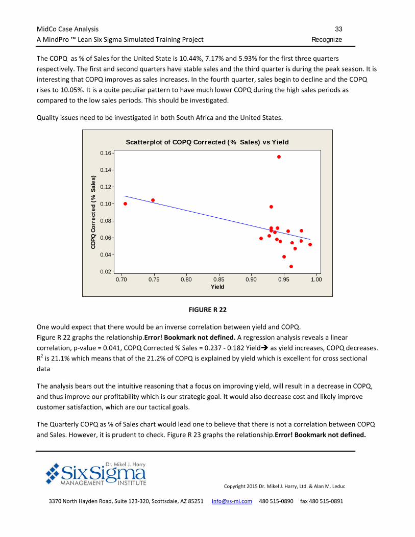
Quality issues need to be investigated in both South Africa and the United States.
1.000.950.900.850.800.750.70
0.16
0.14
0.12
0.10
0.08
0.06
0.04
0.02
Yield
COPQ
Cor
rect
ed (
% S
ales
)
Scatterplot of COPQ Corrected (% Sales) vs Yield
FIGURE R 22
One would expect that there would be an inverse correlation between yield and COPQ.
Figure R 22 graphs the relationship.Error! Bookmark not defined. A regression analysis reveals a linear
correlation, p‐value = 0.041, COPQ Corrected % Sales = 0.237 ‐ 0.182 Yield as yield increases, COPQ decreases.
R2 is 21.1% which means that of the 21.2% of COPQ is explained by yield which is excellent for cross sectional
data
The analysis bears out the intuitive reasoning that a focus on improving yield, will result in a decrease in COPQ,
and thus improve our profitability which is our strategic goal. It would also decrease cost and likely improve
customer satisfaction, which are our tactical goals.
The Quarterly COPQ as % of Sales chart would lead one to believe that there is not a correlation between COPQ
and Sales. However, it is prudent to check. Figure R 23 graphs the relationship.Error! Bookmark not defined.
MidCo Case Analysis 34
A MindPro ™ Lean Six Sigma Simulated Training Project Recognize
Copyright 2015 Dr. Mikel J. Harry, Ltd. & Alan M. Leduc
3370 North Hayden Road, Suite 123‐320, Scottsdale, AZ 85251 info@ss‐mi.com 480 515‐0890 fax 480 515‐0891
50000004000000300000020000001000000
0.16
0.14
0.12
0.10
0.08
0.06
0.04
0.02
Sales $
COPQ
Cor
rect
ed (
% S
ales
)
Scatterplot of COPQ Corrected (% Sales) vs Sales $
FIGURE R 23
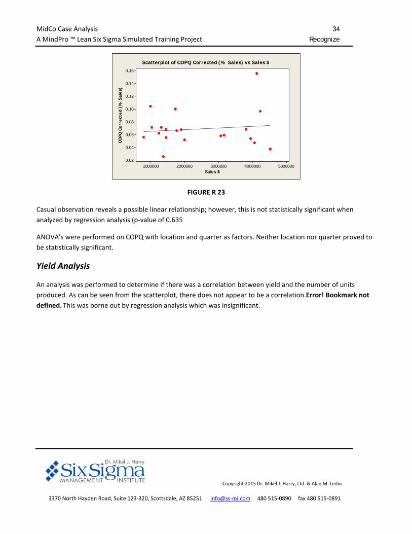
Casual observation reveals a possible linear relationship; however, this is not statistically significant when
analyzed by regression analysis (p‐value of 0.635
ANOVA’s were performed on COPQ with location and quarter as factors. Neither location nor quarter proved to
be statistically significant.
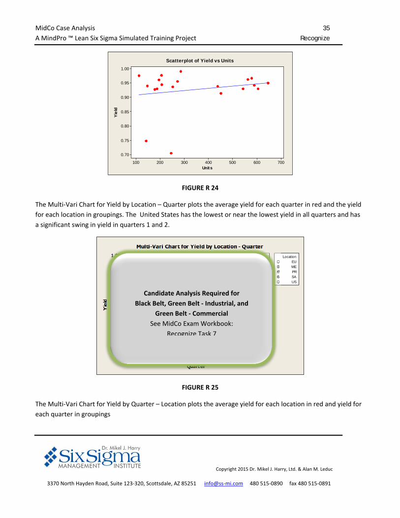
Yield Analysis
An analysis was performed to determine if there was a correlation between yield and the number of units
produced. As can be seen from the scatterplot, there does not appear to be a correlation.Error! Bookmark not
defined. This was borne out by regression analysis which was insignificant.
MidCo Case Analysis 35
A MindPro ™ Lean Six Sigma Simulated Training Project Recognize
Copyright 2015 Dr. Mikel J. Harry, Ltd. & Alan M. Leduc
3370 North Hayden Road, Suite 123‐320, Scottsdale, AZ 85251 info@ss‐mi.com 480 515‐0890 fax 480 515‐0891
700600500400300200100
1.00
0.95
0.90
0.85
0.80
0.75
0.70
Units
Yie
ld
Scatterplot of Yield vs Units
FIGURE R 24
The Multi‐Vari Chart for Yield by Location – Quarter plots the average yield for each quarter in red and the yield
for each location in groupings. The United States has the lowest or near the lowest yield in all quarters and has
a significant swing in yield in quarters 1 and 2.
Quarter
Yie
ld
4321
1.00
0.95
0.90
0.85
0.80
0.75
0.70
Location
US
EUMEPRSA
Multi-Vari Chart for Yield by Location - Quarter
FIGURE R 25
The Multi‐Vari Chart for Yield by Quarter – Location plots the average yield for each location in red and yield for
each quarter in groupings
Candidate Analysis Required for
Black Belt, Green Belt ‐ Industrial, and
Green Belt ‐ Commercial
See MidCo Exam Workbook:
Recognize Task 7
MidCo Case Analysis 36
A MindPro ™ Lean Six Sigma Simulated Training Project Recognize
Copyright 2015 Dr. Mikel J. Harry, Ltd. & Alan M. Leduc
3370 North Hayden Road, Suite 123‐320, Scottsdale, AZ 85251 info@ss‐mi.com 480 515‐0890 fax 480 515‐0891
Location
Yie
ld
USSAPRMEEU
1.00
0.95
0.90
0.85
0.80
0.75
0.70
Quarter1234
Multi-Vari Chart for Yield by Quarter - Location
FIGURE R 26
An analysis of variance (ANOVA) using Yield as the response and Location as a factor and a similar analysis using
Yield as the response and quarter as the factor were performed.
Candidate Conclusions
In terms of Yield which location has the strongest influence
on the Multi‐vari Chart conclusions? Why?
Candidate Analysis Required for
Black Belt, Green Belt ‐ Industrial, and
Green Belt ‐ Commercial
See MidCo Exam Workbook:
Recognize Task 7
Candidate Analysis Required for
Black Belt, Green Belt ‐ Industrial, and
Green Belt ‐ Commercial
See MidCo Exam Workbook:
Recognize Task 7
MidCo Case Analysis 37
A MindPro ™ Lean Six Sigma Simulated Training Project Recognize
Copyright 2015 Dr. Mikel J. Harry, Ltd. & Alan M. Leduc
3370 North Hayden Road, Suite 123‐320, Scottsdale, AZ 85251 info@ss‐mi.com 480 515‐0890 fax 480 515‐0891
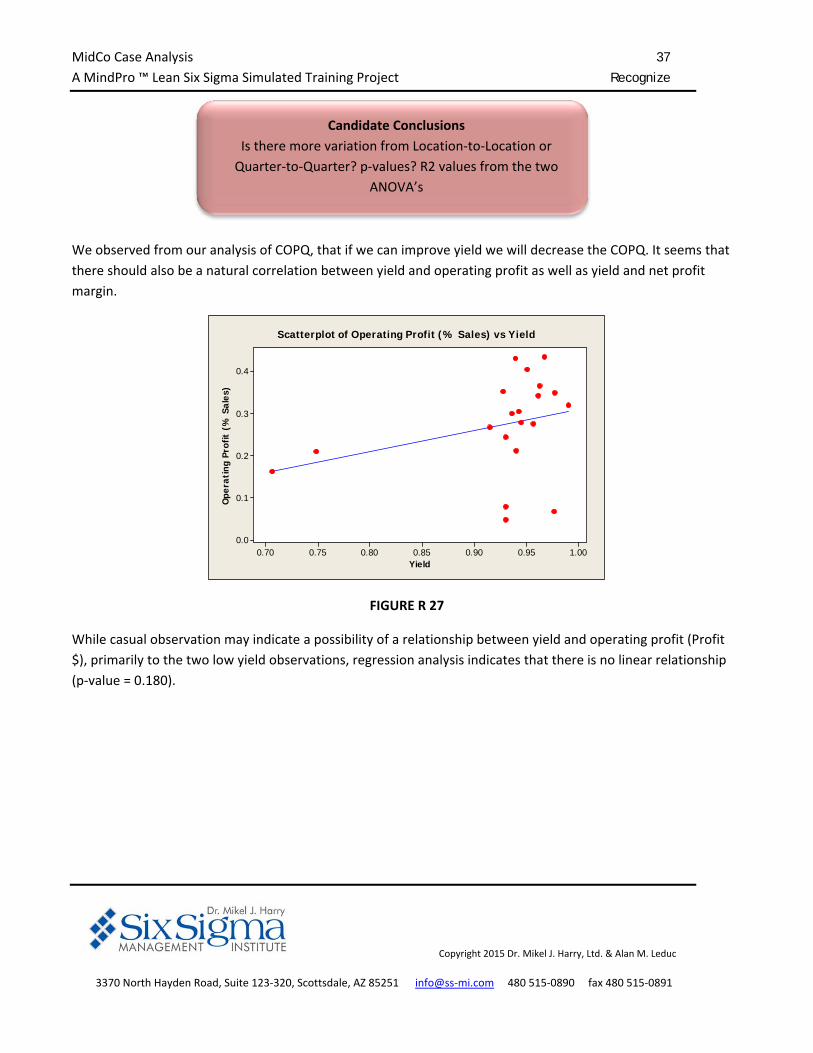
We observed from our analysis of COPQ, that if we can improve yield we will decrease the COPQ. It seems that
there should also be a natural correlation between yield and operating profit as well as yield and net profit
margin.
1.000.950.900.850.800.750.70
0.4
0.3
0.2
0.1
0.0
Yield
Ope
rati
ng P
rofit
(%
Sal
es)
Scatterplot of Operating Profit (% Sales) vs Yield
FIGURE R 27
While casual observation may indicate a possibility of a relationship between yield and operating profit (Profit
$), primarily to the two low yield observations, regression analysis indicates that there is no linear relationship
(p‐value = 0.180).
Candidate Conclusions
Is there more variation from Location‐to‐Location or
Quarter‐to‐Quarter? p‐values? R2 values from the two
ANOVA’s
MidCo Case Analysis 38
A MindPro ™ Lean Six Sigma Simulated Training Project Recognize
Copyright 2015 Dr. Mikel J. Harry, Ltd. & Alan M. Leduc
3370 North Hayden Road, Suite 123‐320, Scottsdale, AZ 85251 info@ss‐mi.com 480 515‐0890 fax 480 515‐0891
1.000.950.900.850.800.750.70
0.14
0.12
0.10
0.08
0.06
0.04
0.02
Yield
Net
Prof
it M
argi
n
Scatterplot of Net Profit Margin vs Yield
FIGURE R 28
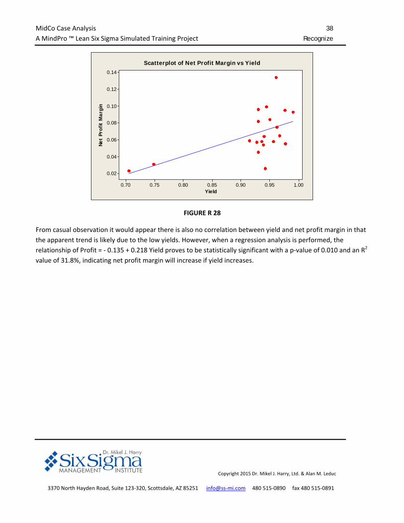
From casual observation it would appear there is also no correlation between yield and net profit margin in that
the apparent trend is likely due to the low yields. However, when a regression analysis is performed, the
relationship of Profit = ‐ 0.135 + 0.218 Yield proves to be statistically significant with a p‐value of 0.010 and an R2
value of 31.8%, indicating net profit margin will increase if yield increases.
MidCo Case Analysis 39
A MindPro ™ Lean Six Sigma Simulated Training Project Recognize
Copyright 2015 Dr. Mikel J. Harry, Ltd. & Alan M. Leduc
3370 North Hayden Road, Suite 123‐320, Scottsdale, AZ 85251 info@ss‐mi.com 480 515‐0890 fax 480 515‐0891
Cost Analysis
MidCo requested an analysis of Cost$ to determine if there was a difference in the variances and means of Cost
$ in the first half of the year as compared to the last half of the year. A test for equal variances was performed in
Minitab using both the F‐test and the Lavene’s Test The graph is shown in Figure R 29.
1
0
225000020000001750000150000012500001000000750000500000
Bi-
Ann
ual
95% Bonferroni Confidence Intervals for StDevs
1
0
350000030000002500000200000015000001000000
Bi-
Ann
ual
Cost $
Test Statistic 0.38P-Value 0.166
Test Statistic 0.33P-Value 0.575
F-Test
Levene's Test
Test for Equal Variances for Cost $
FIGURE R 29
Candidate Analysis Required for
Black Belt and Green Belt ‐ Commercial
See MidCo Exam Workbook:
Recognize Task 9
Candidate Conclusions
Is there a statistical difference in the variances of Cost $
during the first half of the year when compared to the
second half?
MidCo Case Analysis 40
A MindPro ™ Lean Six Sigma Simulated Training Project Recognize
Copyright 2015 Dr. Mikel J. Harry, Ltd. & Alan M. Leduc
3370 North Hayden Road, Suite 123‐320, Scottsdale, AZ 85251 info@ss‐mi.com 480 515‐0890 fax 480 515‐0891
A two‐sample t‐test was performed using Minitab . The graph is show in
Figure R 30.
10
3500000
3000000
2500000
2000000
1500000
1000000
Bi-Annual
Cost
$
Individual Value Plot of Cost $ vs Bi-Annual
FIGURE R 30
Candidate Analysis Required for
Black Belt, Green Belt ‐ Industrial, and
Green Belt ‐ Commercial
See MidCo Exam Workbook:
Recognize Task 10
Candidate Conclusions
Is there a statistical difference in the means of Cost $
during the first half of the year when compared to the
second half?
MidCo Case Analysis 41
A MindPro ™ Lean Six Sigma Simulated Training Project
Copyright 2015 Dr. Mikel J. Harry, Ltd. & Alan M. Leduc
3370 North Hayden Road, Suite 123‐320, Scottsdale, AZ 85251 info@ss‐mi.com 480 515‐0890 fax 480 515‐0891
DEFINE
What product characteristics must be isolated and improved?
Summary
Analysis of the CTQ data provided by MidCo indicates that the United States facility has four
CTQ’s (1, 2, 3, and 7) that should be considered for isolation and improvement. If these four
CTQ’s can be brought to a 99.60% first time yield, the rolled throughput yield will increase from
88.00% to 99.26% and the short term sigma will improve from 3.74 Sigma to 4.17 Sigma which
would be a significant improvement and take us toward our strategic goal of increased
productivity and our tactical goals of decreased cost and improved customer satisfaction.
However, this is MidCo’s first Six Sigma project and they ask that we provide them with an
improvement estimate based only upon looking at only the two CTQ’s that had the highest
failure rate, CTQ’s 1 and 2. Based upon the what‐if analysis, MidCo was advised that bringing
CTQ’s 1 and 2 to a 99.60% first time yield and leaving the remaining eight CTQ’s at status quo
would provide a rolled throughput yield of 94.34% and a short term sigma of 4.03.
MidCo advised that they would prefer to limit the Measurement Phase to CTQ’s 1 and 2.
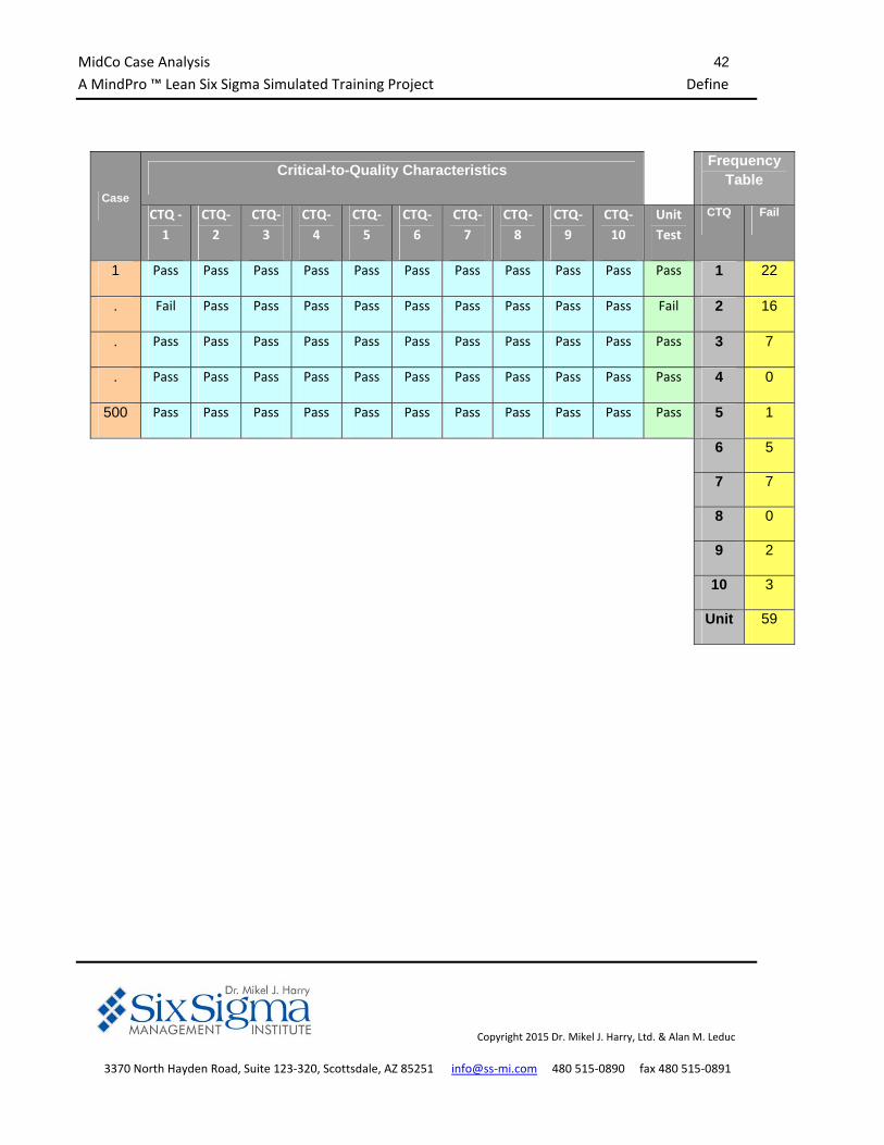
The Recognize Phase indicated that we should concentrate on yield as the performance metric to drive Six Sigma
and that our focus should be on the United States facility. MidCo provided data in the following format for the
United States facility.
MidCo Case Analysis 42
A MindPro ™ Lean Six Sigma Simulated Training Project Define
Copyright 2015 Dr. Mikel J. Harry, Ltd. & Alan M. Leduc
3370 North Hayden Road, Suite 123‐320, Scottsdale, AZ 85251 info@ss‐mi.com 480 515‐0890 fax 480 515‐0891
Case
Critical-to-Quality Characteristics
Frequency Table
CTQ ‐
1
CTQ‐
2
CTQ‐
3
CTQ‐
4
CTQ‐
5
CTQ‐
6
CTQ‐
7
CTQ‐
8
CTQ‐
9
CTQ‐
10
Unit
Test
CTQ Fail
1 Pass Pass Pass Pass Pass Pass Pass Pass Pass Pass Pass 1 22
. Fail Pass Pass Pass Pass Pass Pass Pass Pass Pass Fail 2 16
. Pass Pass Pass Pass Pass Pass Pass Pass Pass Pass Pass 3 7
. Pass Pass Pass Pass Pass Pass Pass Pass Pass Pass Pass 4 0
500 Pass Pass Pass Pass Pass Pass Pass Pass Pass Pass Pass 5 1
6 5
7 7
8 0
9 2
10 3
Unit 59
MidCo Case Analysis 43
A MindPro ™ Lean Six Sigma Simulated Training Project Define
Copyright 2015 Dr. Mikel J. Harry, Ltd. & Alan M. Leduc
3370 North Hayden Road, Suite 123‐320, Scottsdale, AZ 85251 info@ss‐mi.com 480 515‐0890 fax 480 515‐0891
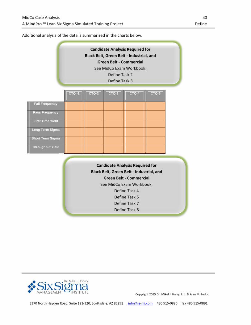
Additional analysis of the data is summarized in the charts below.
CTQ -1 CTQ-2 CTQ-3 CTQ-4 CTQ-5
Fail Frequency
Pass Frequency
First Time Yield
Long Term Sigma
Short Term Sigma
Throughput Yield
Candidate Analysis Required for
Black Belt, Green Belt ‐ Industrial, and
Green Belt ‐ Commercial
See MidCo Exam Workbook:
Define Task 2
Define Task 3
Candidate Analysis Required for
Black Belt, Green Belt ‐ Industrial, and
Green Belt ‐ Commercial
See MidCo Exam Workbook:
Define Task 4
Define Task 5
Define Task 7
Define Task 8
MidCo Case Analysis 44
A MindPro ™ Lean Six Sigma Simulated Training Project Define
Copyright 2015 Dr. Mikel J. Harry, Ltd. & Alan M. Leduc
3370 North Hayden Road, Suite 123‐320, Scottsdale, AZ 85251 info@ss‐mi.com 480 515‐0890 fax 480 515‐0891
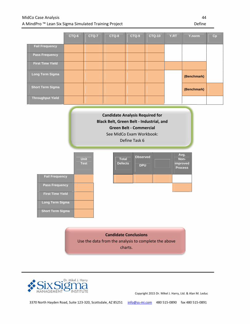
CTQ-6 CTQ-7 CTQ-8 CTQ-9 CTQ-10 Y.RT Y.norm Cp
Fail Frequency
Pass Frequency
First Time Yield
Long Term Sigma
(Benchmark)
Short Term Sigma
(Benchmark)
Throughput Yield
Unit Test
Total Defects
Observed
DPU
Avg. Non-
improved Process
Fail Frequency
Pass Frequency
First Time Yield
Long Term Sigma
Short Term Sigma
Candidate Analysis Required for
Black Belt, Green Belt ‐ Industrial, and
Green Belt ‐ Commercial
See MidCo Exam Workbook:
Define Task 6
Candidate Conclusions
Use the data from the analysis to complete the above
charts.
MidCo Case Analysis 45
A MindPro ™ Lean Six Sigma Simulated Training Project Define
Copyright 2015 Dr. Mikel J. Harry, Ltd. & Alan M. Leduc
3370 North Hayden Road, Suite 123‐320, Scottsdale, AZ 85251 info@ss‐mi.com 480 515‐0890 fax 480 515‐0891
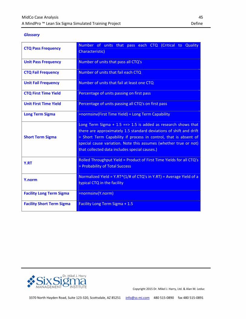
Glossary
CTQ Pass Frequency Number of units that pass each CTQ (Critical to Quality
Characteristic)
Unit Pass Frequency Number of units that pass all CTQ's
CTQ Fail Frequency Number of units that fail each CTQ
Unit Fail Frequency Number of units that fail at least one CTQ
CTQ First Time Yield Percentage of units passing on first pass
Unit First Time Yield Percentage of units passing all CTQ's on first pass
Long Term Sigma =normsinv(First Time Yield) = Long Term Capability
Short Term Sigma
Long Term Sigma + 1.5 ==> 1.5 is added as research shows that
there are approximately 1.5 standard deviations of shift and drift
= Short Term Capability if process in control, that is absent of
special cause variation. Note this assumes (whether true or not)
that collected data includes special causes.)
Y.RT Rolled Throughput Yield = Product of First Time Yields for all CTQ's
= Probability of Total Success
Y.norm Normalized Yield = Y.RT^(1/# of CTQ's in Y.RT) = Average Yield of a
typical CTQ in the facility
Facility Long Term Sigma =normsinv(Y.norm)
Facility Short Term Sigma Facility Long Term Sigma + 1.5
MidCo Case Analysis 46
A MindPro ™ Lean Six Sigma Simulated Training Project Define
Copyright 2015 Dr. Mikel J. Harry, Ltd. & Alan M. Leduc
3370 North Hayden Road, Suite 123‐320, Scottsdale, AZ 85251 info@ss‐mi.com 480 515‐0890 fax 480 515‐0891
MidCo is operating at 3.741 Short Term Sigma. To put this number in perspective, 1900 to 1950 manufacturing
was about 3 Sigma (66,807 defects per million); the average company today operates at about 4 Sigma (6,210
defects per million); world class companies operate at about 5 Sigma (233 defect per million); and the ultimate
goal is to operate at 6 Sigma (3.4 defects per million). MidCo is operating at a level below average.
MidCo had specific interest in CTQ‐5 for which 499 of the 500 Unit Passed, a 98.000% First‐Time Yield.
Specifically they wanted to know the confidence interval on the Yield.
Candidate Conclusions
How many Units were tested? How many Units passed all
CTQ’s? How many Units failed only one CTQ? How many
Units failed more than one CTQ?
Candidate Analysis Required for
Black Belt, Green Belt ‐ Industrial, and
Green Belt ‐ Commercial
See MidCo Exam Workbook:
Define Task 1
Candidate Conclusions
What is the confidence on CTQ‐5 Yield?
Candidate Analysis Required for
Black Belt, Green Belt ‐ Industrial, and
Green Belt ‐ Commercial
See MidCo Exam Workbook:
Define Task 11
MidCo Case Analysis 47
A MindPro ™ Lean Six Sigma Simulated Training Project Define
Copyright 2015 Dr. Mikel J. Harry, Ltd. & Alan M. Leduc
3370 North Hayden Road, Suite 123‐320, Scottsdale, AZ 85251 info@ss‐mi.com 480 515‐0890 fax 480 515‐0891
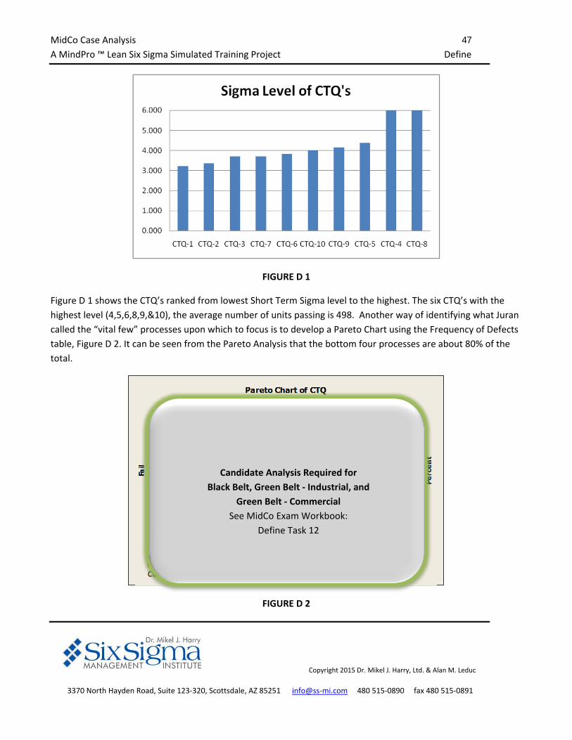
FIGURE D 1
Figure D 1 shows the CTQ’s ranked from lowest Short Term Sigma level to the highest. The six CTQ’s with the
highest level (4,5,6,8,9,&10), the average number of units passing is 498. Another way of identifying what Juran
called the “vital few” processes upon which to focus is to develop a Pareto Chart using the Frequency of Defects
table, Figure D 2. It can be seen from the Pareto Analysis that the bottom four processes are about 80% of the
total.
Fail 22 16 7 7 5 3 3Percent 34.9 25.4 11.1 11.1 7.9 4.8 4.8Cum % 34.9 60.3 71.4 82.5 90.5 95.2 100.0
CTQ Other1067321
70
60
50
40
30
20
10
0
100
80
60
40
20
0
Fail
Perc
ent
Pareto Chart of CTQ
FIGURE D 2
Candidate Analysis Required for
Black Belt, Green Belt ‐ Industrial, and
Green Belt ‐ Commercial
See MidCo Exam Workbook:
Define Task 12
MidCo Case Analysis 48
A MindPro ™ Lean Six Sigma Simulated Training Project Define
Copyright 2015 Dr. Mikel J. Harry, Ltd. & Alan M. Leduc
3370 North Hayden Road, Suite 123‐320, Scottsdale, AZ 85251 info@ss‐mi.com 480 515‐0890 fax 480 515‐0891
An analysis was done to determine the number of cases in which CTQ‐1 “Passed” but the Unit “Failed.”
Candidate Conclusions
Which CTQ has the poorest performing process? Which
process provides the most leverage for improvement?
What are the vital few CTQ’s
Candidate Analysis Required for
Black Belt and Green Belt ‐ Commercial
See MidCo Exam Workbook:
Define Task 9
Define Task 10
Candidate Conclusions
In how many and what percent of the cases did the Unit
Test fail while CTQ‐1 passed? In how many and what
percent of cases did the Unit Test fail when CTQ‐1 also
failed?
MidCo Case Analysis 49
A MindPro ™ Lean Six Sigma Simulated Training Project Define
Copyright 2015 Dr. Mikel J. Harry, Ltd. & Alan M. Leduc
3370 North Hayden Road, Suite 123‐320, Scottsdale, AZ 85251 info@ss‐mi.com 480 515‐0890 fax 480 515‐0891
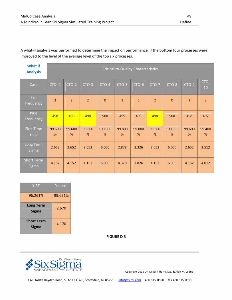
A what‐if analysis was performed to determine the impact on performance, if the bottom four processes were
improved to the level of the average level of the top six processes.
What if
Analysis Critical‐to‐Quality Characteristics
Case CTQ ‐1 CTQ‐2 CTQ‐3 CTQ‐4 CTQ‐5 CTQ‐6 CTQ‐7 CTQ‐8 CTQ‐9 CTQ‐
10
Fail
Frequency 2 2 2 0 1 5 2 0 2 3
Pass
Frequency 498 498 498 500 499 495 498 500 498 497
First Time
Yield
99.600
%
99.600
%
99.600
%
100.000
%
99.800
%
99.000
%
99.600
%
100.000
%
99.600
%
99.400
%
Long Term
Sigma 2.652 2.652 2.652 6.000 2.878 2.326 2.652 6.000 2.652 2.512
Short Term
Sigma 4.152 4.152 4.152 6.000 4.378 3.826 4.152 6.000 4.152 4.012
Y.RT Y.norm
96.261% 99.621%
Long Term
Sigma 2.670
Short Term
Sigma 4.170
FIGURE D 3
MidCo Case Analysis 50
A MindPro ™ Lean Six Sigma Simulated Training Project Define
Copyright 2015 Dr. Mikel J. Harry, Ltd. & Alan M. Leduc
3370 North Hayden Road, Suite 123‐320, Scottsdale, AZ 85251 info@ss‐mi.com 480 515‐0890 fax 480 515‐0891
If the pass frequency of the bottom four processes can be increased to 498 (99.6% first time yield), then number
of defects would be decreased from 63 to 19; the rolled throughput yield would increase from 88.003% to
96.261%; and short term sigma would be increased from 3.741 to 4.17 allowing MidCo to move from below
average to above average performance.
What if the next two CTQ’s in the Pareto Chart (6 and 10) were also increased to a 498 Pass Frequency?
Only small additional gains are achieved by focusing on the bottom six processes instead of the bottom four
processes: the number of defects would be decreased to 17 versus 19; the rolled throughput yield would
increase to 97.039% from 96.261%; and short term sigma increases from 4.17 to 4.25. The effort to focus on the
additional two processes does not reap significant additional benefits. Most processes are dynamic, so it would
be best to concentrate only on the bottom four processes and once the process is stable under the new
conditions, consider an additional project CTQ‐6 and CTQ‐10.
MidCo Case Analysis 51
A MindPro ™ Lean Six Sigma Simulated Training Project Define
Copyright 2015 Dr. Mikel J. Harry, Ltd. & Alan M. Leduc
3370 North Hayden Road, Suite 123‐320, Scottsdale, AZ 85251 info@ss‐mi.com 480 515‐0890 fax 480 515‐0891
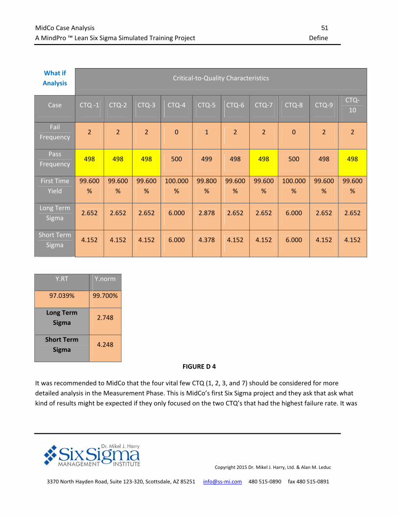
What if
Analysis Critical‐to‐Quality Characteristics
Case CTQ ‐1 CTQ‐2 CTQ‐3 CTQ‐4 CTQ‐5 CTQ‐6 CTQ‐7 CTQ‐8 CTQ‐9 CTQ‐
10
Fail
Frequency 2 2 2 0 1 2 2 0 2 2
Pass
Frequency 498 498 498 500 499 498 498 500 498 498
First Time
Yield
99.600
%
99.600
%
99.600
%
100.000
%
99.800
%
99.600
%
99.600
%
100.000
%
99.600
%
99.600
%
Long Term
Sigma 2.652 2.652 2.652 6.000 2.878 2.652 2.652 6.000 2.652 2.652
Short Term
Sigma 4.152 4.152 4.152 6.000 4.378 4.152 4.152 6.000 4.152 4.152
Y.RT Y.norm
97.039% 99.700%
Long Term
Sigma 2.748
Short Term
Sigma 4.248
FIGURE D 4
It was recommended to MidCo that the four vital few CTQ (1, 2, 3, and 7) should be considered for more
detailed analysis in the Measurement Phase. This is MidCo’s first Six Sigma project and they ask that ask what
kind of results might be expected if they only focused on the two CTQ’s that had the highest failure rate. It was
MidCo Case Analysis 52
A MindPro ™ Lean Six Sigma Simulated Training Project Define
Copyright 2015 Dr. Mikel J. Harry, Ltd. & Alan M. Leduc
3370 North Hayden Road, Suite 123‐320, Scottsdale, AZ 85251 info@ss‐mi.com 480 515‐0890 fax 480 515‐0891
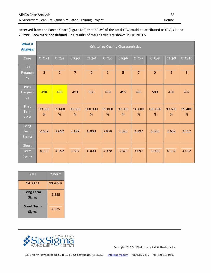
observed from the Pareto Chart (Figure D 2) that 60.3% of the total CTQ could be attributed to CTQ’s 1 and
2.Error! Bookmark not defined. The results of the analysis are shown in Figure D 5.
What if
Analysis Critical‐to‐Quality Characteristics
Case CTQ ‐1 CTQ‐2 CTQ‐3 CTQ‐4 CTQ‐5 CTQ‐6 CTQ‐7 CTQ‐8 CTQ‐9 CTQ‐10
Fail
Frequen
cy
2 2 7 0 1 5 7 0 2 3
Pass
Frequen
cy
498 498 493 500 499 495 493 500 498 497
First
Time
Yield
99.600
%
99.600
%
98.600
%
100.000
%
99.800
%
99.000
%
98.600
%
100.000
%
99.600
%
99.400
%
Long
Term
Sigma
2.652 2.652 2.197 6.000 2.878 2.326 2.197 6.000 2.652 2.512
Short
Term
Sigma
4.152 4.152 3.697 6.000 4.378 3.826 3.697 6.000 4.152 4.012
Y.RT Y.norm
94.337% 99.422%
Long Term
Sigma 2.525
Short Term
Sigma 4.025
MidCo Case Analysis 53
A MindPro ™ Lean Six Sigma Simulated Training Project Define
Copyright 2015 Dr. Mikel J. Harry, Ltd. & Alan M. Leduc
3370 North Hayden Road, Suite 123‐320, Scottsdale, AZ 85251 info@ss‐mi.com 480 515‐0890 fax 480 515‐0891
FIGURE D 5
Based upon the what‐if analysis, MidCo was advised that bringing CTQ’s 1 and 2 to a 99.60% first time yield and
leaving the remaining eight CTQ’s at status quo would provide a rolled throughput yield of 94.337% and a short
term sigma of 4.03. MidCo advised that they would prefer to limit the Measurement Phase to CTQ’s 1 and 2.
MidCo Case Analysis 54
A MindPro ™ Lean Six Sigma Simulated Training Project
Copyright 2015 Dr. Mikel J. Harry, Ltd. & Alan M. Leduc
3370 North Hayden Road, Suite 123‐320, Scottsdale, AZ 85251 info@ss‐mi.com 480 515‐0890 fax 480 515‐0891
Measure
What is the actual and potential capability of the core CTQ’s?
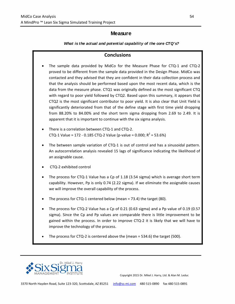
Conclusions
The sample data provided by MidCo for the Measure Phase for CTQ‐1 and CTQ‐2
proved to be different from the sample data provided in the Design Phase. MidCo was
contacted and they advised that they are confident in their data collection process and
that the analysis should be performed based upon the most recent data, which is the
data from the measure phase. CTQ1 was originally defined as the most significant CTQ
with regard to poor yield followed by CTQ2. Based upon this summary, it appears that
CTQ2 is the most significant contributor to poor yield. It is also clear that Unit Yield is
significantly deteriorated from that of the define stage with first time yield dropping
from 88.20% to 84.00% and the short term sigma dropping from 2.69 to 2.49. It is
apparent that it is important to continue with the six sigma analysis.
There is a correlation between CTQ‐1 and CTQ‐2.
CTQ‐1 Value = 172 ‐ 0.185 CTQ‐2 Value (p‐value = 0.000; R2 = 53.6%)
The between sample variation of CTQ‐1 is out of control and has a sinusoidal pattern.
An autocorrelation analysis revealed 15 lags of significance indicating the likelihood of
an assignable cause.
CTQ‐2 exhibited control
The process for CTQ‐1 Value has a Cp of 1.18 (3.54 sigma) which is average short term
capability. However, Pp is only 0.74 (2.22 sigma). If we eliminate the assignable causes
we will improve the overall capability of the process.
The process for CTQ‐1 centered below (mean = 73.4) the target (80).
The process for CTQ‐2 Value has a Cp of 0.21 (0.63 sigma) and a Pp value of 0.19 (0.57
sigma). Since the Cp and Pp values are comparable there is little improvement to be
gained within the process. In order to improve CTQ‐2 it is likely that we will have to
improve the technology of the process.
The process for CTQ‐2 is centered above the (mean = 534.6) the target (500).
MidCo Case Analysis 55
A MindPro ™ Lean Six Sigma Simulated Training Project Measure
Copyright 2015 Dr. Mikel J. Harry, Ltd. & Alan M. Leduc
3370 North Hayden Road, Suite 123‐320, Scottsdale, AZ 85251 info@ss‐mi.com 480 515‐0890 fax 480 515‐0891
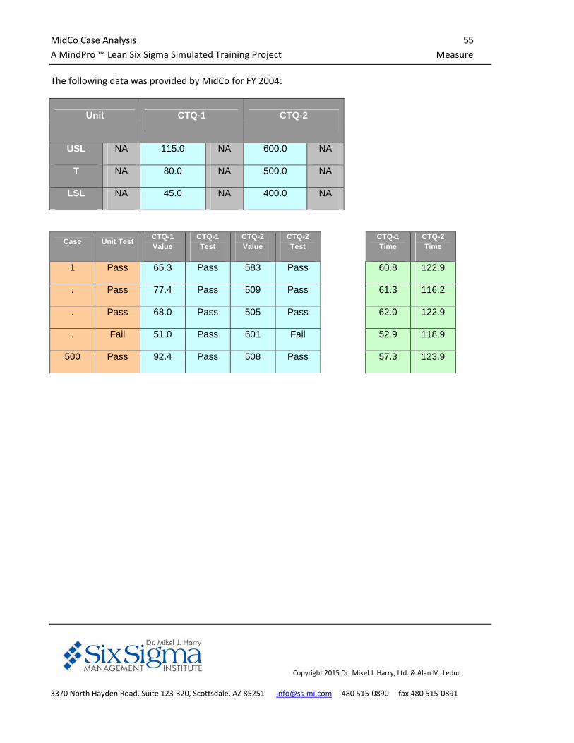
The following data was provided by MidCo for FY 2004:
Unit CTQ-1 CTQ-2
USL NA 115.0 NA 600.0 NA
T NA 80.0 NA 500.0 NA
LSL NA 45.0 NA 400.0 NA
Case Unit Test CTQ-1 Value
CTQ-1 Test
CTQ-2 Value
CTQ-2 Test
CTQ-1 Time
CTQ-2 Time
1 Pass 65.3 Pass 583 Pass 60.8 122.9
. Pass 77.4 Pass 509 Pass 61.3 116.2
. Pass 68.0 Pass 505 Pass 62.0 122.9
. Fail 51.0 Pass 601 Fail 52.9 118.9
500 Pass 92.4 Pass 508 Pass 57.3 123.9
MidCo Case Analysis 56
A MindPro ™ Lean Six Sigma Simulated Training Project Measure
Copyright 2015 Dr. Mikel J. Harry, Ltd. & Alan M. Leduc
3370 North Hayden Road, Suite 123‐320, Scottsdale, AZ 85251 info@ss‐mi.com 480 515‐0890 fax 480 515‐0891
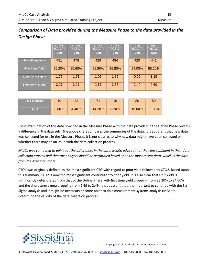
Comparison of Data provided during the Measure Phase to the data provided in the
Design Phase
CTQ-1 Measure
Data
CTQ-1 Define Data
CTQ-2 Measure
Data
CTQ-2 Define Data
Unit Measure
Data
Unit Define Data
Pass Frequency 481 478 429 484 420 441
First Time Yield 96.20% 95.60% 85.80% 96.80% 84.00% 88.20%
Long Term Sigma 1.77 1.71 1.07 1.85 0.99 1.19
Short Term Sigma 3.27 3.21 2.57 3.35 2.49 2.69
Fail Frequency 19 22 71 16 80 59
Fail % 3.80% 4.40% 14.20% 3.20% 16.00% 11.80%
Close examination of the data provided in the Measure Phase with the data provided in the Define Phase reveals
a difference in the data sets. The above chart compares the summaries of the data. It is apparent that new data
was collected for use in the Measure Phase. It is not clear as to why new data might have been collected or
whether there may be an issue with the data collection process.
MidCo was contacted to point out the differences in the data. MidCo advised that they are confident in their data
collection process and that the analysis should be performed based upon the most recent data, which is the data
from the Measure Phase.
CTQ1 was originally defined as the most significant CTQ with regard to poor yield followed by CTQ2. Based upon
this summary, CTQ2 is now the most significant contributor to poor yield. It is also clear that Unit Yield is
significantly deteriorated from that of the Define Phase with first time yield dropping from 88.20% to 84.00%
and the short term sigma dropping from 2.69 to 2.49. It is apparent that it is important to continue with the Six
Sigma analysis and it might be necessary at some point to do a measurement systems analysis (MSA) to
determine the validity of the data collection process.
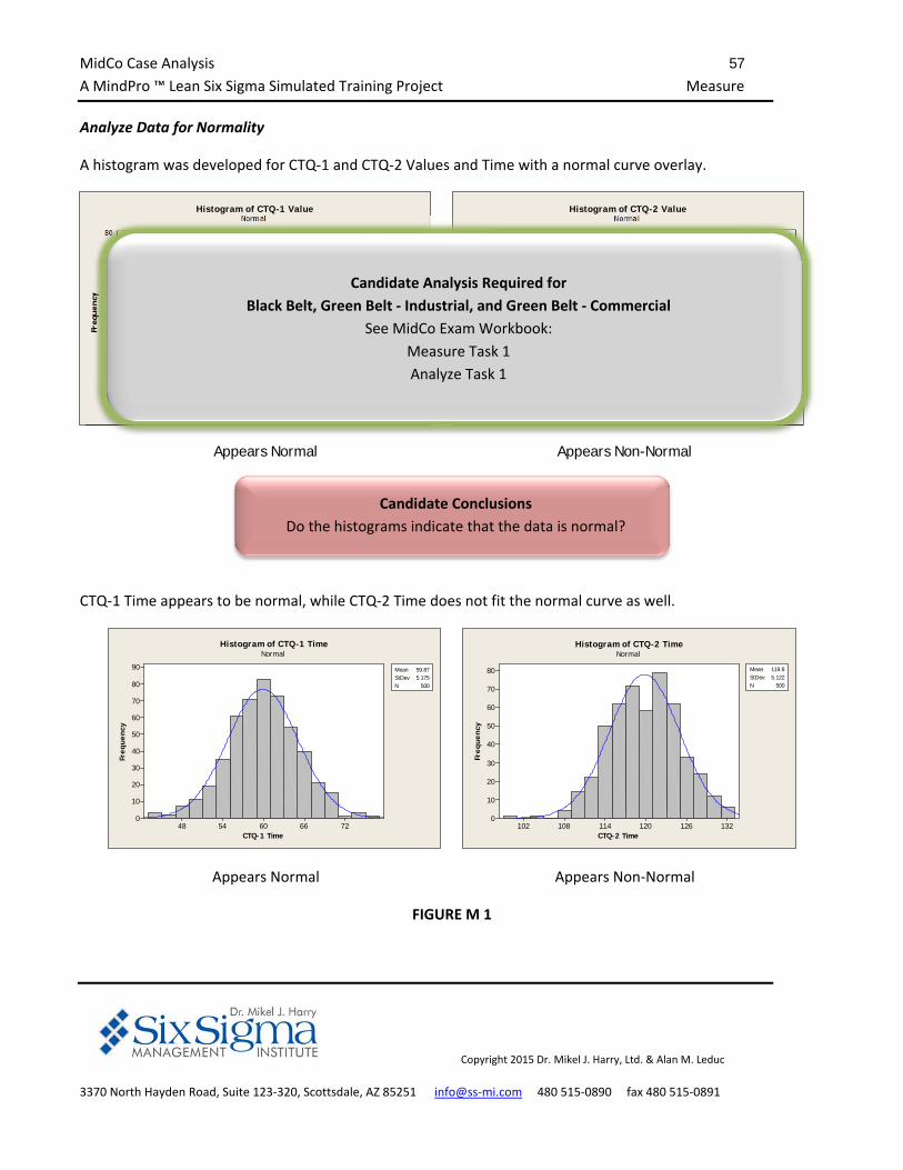
MidCo Case Analysis 57
A MindPro ™ Lean Six Sigma Simulated Training Project Measure
Copyright 2015 Dr. Mikel J. Harry, Ltd. & Alan M. Leduc
3370 North Hayden Road, Suite 123‐320, Scottsdale, AZ 85251 info@ss‐mi.com 480 515‐0890 fax 480 515‐0891
Analyze Data for Normality
A histogram was developed for CTQ‐1 and CTQ‐2 Values and Time with a normal curve overlay.
1201059075604530
80
70
60
50
40
30
20
10
0
CTQ-1 Value
Freq
uenc
y
Mean 73.37StDev 15.84N 500
Histogram of CTQ-1 ValueNormal
780720660600540480420
70
60
50
40
30
20
10
0
CTQ-2 Value
Freq
uenc
y
Mean 534.6StDev 62.79N 500
Histogram of CTQ-2 ValueNormal
Appears Normal Appears Non-Normal
CTQ‐1 Time appears to be normal, while CTQ‐2 Time does not fit the normal curve as well.
7266605448
90
80
70
60
50
40
30
20
10
0
CTQ-1 Time
Freq
uenc
y
Mean 59.87StDev 5.175N 500
Histogram of CTQ-1 TimeNormal
132126120114108102
80
70
60
50
40
30
20
10
0
CTQ-2 Time
Freq
uenc
y
Mean 119.8StDev 5.122N 500
Histogram of CTQ-2 TimeNormal
Appears Normal Appears Non‐Normal
FIGURE M 1
Candidate Conclusions
Do the histograms indicate that the data is normal?
Candidate Analysis Required for
Black Belt, Green Belt ‐ Industrial, and Green Belt ‐ Commercial
See MidCo Exam Workbook:
Measure Task 1
Analyze Task 1
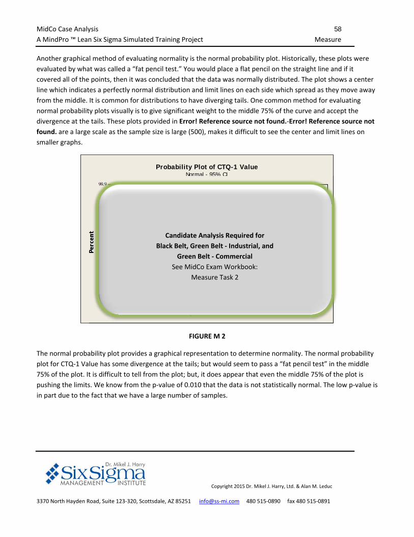
MidCo Case Analysis 58
A MindPro ™ Lean Six Sigma Simulated Training Project Measure
Copyright 2015 Dr. Mikel J. Harry, Ltd. & Alan M. Leduc
3370 North Hayden Road, Suite 123‐320, Scottsdale, AZ 85251 info@ss‐mi.com 480 515‐0890 fax 480 515‐0891
Another graphical method of evaluating normality is the normal probability plot. Historically, these plots were
evaluated by what was called a “fat pencil test.” You would place a flat pencil on the straight line and if it
covered all of the points, then it was concluded that the data was normally distributed. The plot shows a center
line which indicates a perfectly normal distribution and limit lines on each side which spread as they move away
from the middle. It is common for distributions to have diverging tails. One common method for evaluating
normal probability plots visually is to give significant weight to the middle 75% of the curve and accept the
divergence at the tails. These plots provided in Error! Reference source not found.‐Error! Reference source not
found. are a large scale as the sample size is large (500), makes it difficult to see the center and limit lines on
smaller graphs.
14012010080604020
99.9
99
9590
80706050403020
10
5
1
0.1
CTQ-1 Value
Perc
ent
Mean 73.37StDev 15.84N 500AD 1.032P-Value 0.010
Probability Plot of CTQ-1 ValueNormal - 95% CI
FIGURE M 2
The normal probability plot provides a graphical representation to determine normality. The normal probability
plot for CTQ‐1 Value has some divergence at the tails; but would seem to pass a “fat pencil test” in the middle
75% of the plot. It is difficult to tell from the plot; but, it does appear that even the middle 75% of the plot is
pushing the limits. We know from the p‐value of 0.010 that the data is not statistically normal. The low p‐value is
in part due to the fact that we have a large number of samples.
Candidate Analysis Required for
Black Belt, Green Belt ‐ Industrial, and
Green Belt ‐ Commercial
See MidCo Exam Workbook:
Measure Task 2
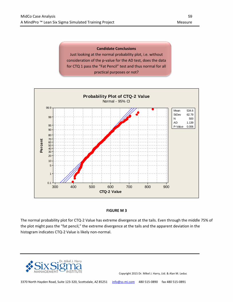
MidCo Case Analysis 59
A MindPro ™ Lean Six Sigma Simulated Training Project Measure
Copyright 2015 Dr. Mikel J. Harry, Ltd. & Alan M. Leduc
3370 North Hayden Road, Suite 123‐320, Scottsdale, AZ 85251 info@ss‐mi.com 480 515‐0890 fax 480 515‐0891
900800700600500400300
99.9
99
9590
80706050403020
10
5
1
0.1
CTQ-2 Value
Perc
ent
Mean 534.6StDev 62.79N 500AD 1.139P-Value 0.006
Probability Plot of CTQ-2 ValueNormal - 95% CI
FIGURE M 3
The normal probability plot for CTQ‐2 Value has extreme divergence at the tails. Even through the middle 75% of
the plot might pass the “fat pencil,” the extreme divergence at the tails and the apparent deviation in the
histogram indicates CTQ‐2 Value is likely non‐normal.
Candidate Conclusions
Just looking at the normal probability plot, i.e. without
consideration of the p‐value for the AD test, does the data
for CTQ 1 pass the “Fat Pencil” test and thus normal for all
practical purposes or not?
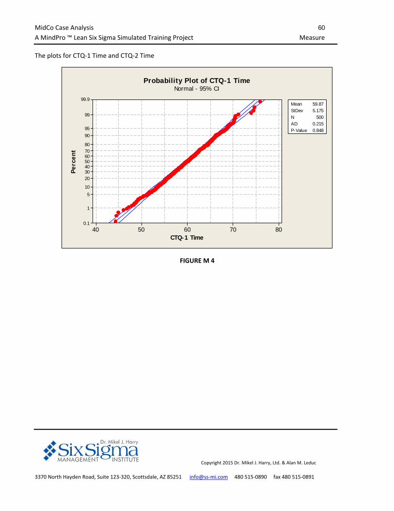
MidCo Case Analysis 60
A MindPro ™ Lean Six Sigma Simulated Training Project Measure
Copyright 2015 Dr. Mikel J. Harry, Ltd. & Alan M. Leduc
3370 North Hayden Road, Suite 123‐320, Scottsdale, AZ 85251 info@ss‐mi.com 480 515‐0890 fax 480 515‐0891
The plots for CTQ‐1 Time and CTQ‐2 Time
8070605040
99.9
99
9590
80706050403020
10
5
1
0.1
CTQ-1 Time
Perc
ent
Mean 59.87StDev 5.175N 500AD 0.215P-Value 0.848
Probability Plot of CTQ-1 TimeNormal - 95% CI
FIGURE M 4
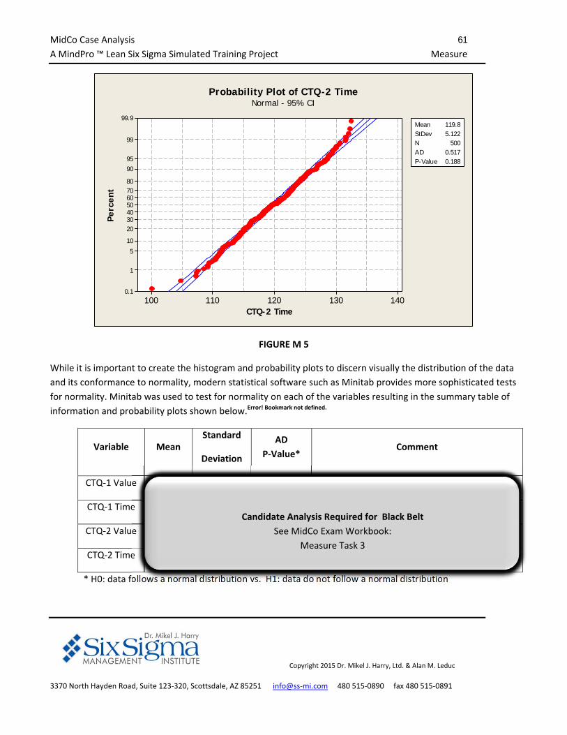
MidCo Case Analysis 61
A MindPro ™ Lean Six Sigma Simulated Training Project Measure
Copyright 2015 Dr. Mikel J. Harry, Ltd. & Alan M. Leduc
3370 North Hayden Road, Suite 123‐320, Scottsdale, AZ 85251 info@ss‐mi.com 480 515‐0890 fax 480 515‐0891
140130120110100
99.9
99
9590
80706050403020
10
5
1
0.1
CTQ-2 Time
Perc
ent
Mean 119.8StDev 5.122N 500AD 0.517P-Value 0.188
Probability Plot of CTQ-2 TimeNormal - 95% CI
FIGURE M 5
While it is important to create the histogram and probability plots to discern visually the distribution of the data
and its conformance to normality, modern statistical software such as Minitab provides more sophisticated tests
for normality. Minitab was used to test for normality on each of the variables resulting in the summary table of
information and probability plots shown below.Error! Bookmark not defined.
Variable Mean Standard
Deviation
AD
P‐Value* Comment
CTQ‐1 Value 73.4 15.8 0.010 Data do not follow a normal distribution
CTQ‐1 Time 59.9 5.2 0.848 Data appear to follow a normal distribution
CTQ‐2 Value 534.6 62.8 0.006 Data do not follow a normal distribution
CTQ‐2 Time 119.8 5.1 0.188 Data appear to follow a normal distribution
* H0: data follows a normal distribution vs. H1: data do not follow a normal distribution
Candidate Analysis Required for Black Belt
See MidCo Exam Workbook:
Measure Task 3
MidCo Case Analysis 62
A MindPro ™ Lean Six Sigma Simulated Training Project Measure
Copyright 2015 Dr. Mikel J. Harry, Ltd. & Alan M. Leduc
3370 North Hayden Road, Suite 123‐320, Scottsdale, AZ 85251 info@ss‐mi.com 480 515‐0890 fax 480 515‐0891
Small deviations in large sample sizes can have a significant impact on the p‐value for normality. Large data sets
provide a lot of power for the test and with certain tests like the Anderson‐Darling test which applies a large
penalty to data points at the extremes, the test may be more sensitive than is important for practical means.
Therefore, it is usually a good idea to look at a histogram of the data when the normality test indicates that the
data is non‐normal. The histograms for CTQ‐1 Value and CTQ‐2 Value are provided below.
The Anderson‐Darling (AD) test is a powerful and extremely sensitive statistical test for determining departures
from a stated distribution. A p‐value below the critical value for the Anderson‐Darling test indicates the data
does not conform to specified distribution. For example if the critical p‐value is 0.05, and the AD p‐value is 0.01,
then the data would be statistically non‐normal.
The Anderson‐Darling test is a powerful test which heavily weights the tails, so it is often acceptable to assume
normality for practical purposes based upon the probability plot passing the “fat pencil test.”
An Anderson‐Darling (AD) test statistic of zero indicates a perfectly normal fit. While the actual AD test statistic
is difficult to interpret, the statistics can be compared. The AD statistic for CTQ‐? Value is _____ and for CTQ‐?
Value is _____. This indicates the CTQ‐? Value is “more (or less) normal” than CTQ‐? Value as is indicated visually
by the probability plot.
Search for Patterns and Correlation
A line chart plots the observations in time sequence and allows the analyst the opportunity to inspect the data
for possible patterns. Line charts created in Excel are shown below:
0.0
50.0
100.0
150.0
1 15 29 43 57 71 85 99 113
127
141
155
169
183
197
211
225
239
253
267
281
295
309
323
337
351
365
379
393
407
421
435
449
463
477
491
Candidate Conclusions
Complete the Chart above and comment as to whether or
not the AD test indicates whether or not the data is
statistically normal.
Candidate Analysis Required for
Black Belt, Green Belt ‐ Industrial, and Green Belt ‐ Commercial
See MidCo Exam Workbook:
Measure Task 4
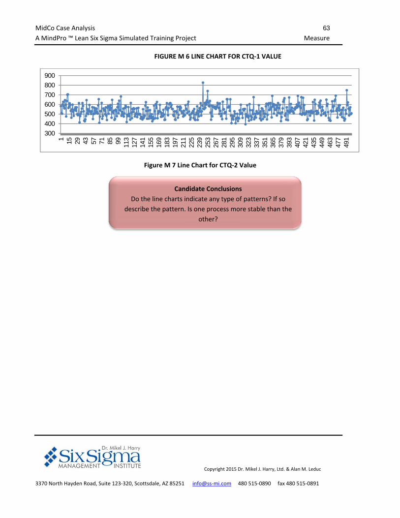
MidCo Case Analysis 63
A MindPro ™ Lean Six Sigma Simulated Training Project Measure
Copyright 2015 Dr. Mikel J. Harry, Ltd. & Alan M. Leduc
3370 North Hayden Road, Suite 123‐320, Scottsdale, AZ 85251 info@ss‐mi.com 480 515‐0890 fax 480 515‐0891
FIGURE M 6 LINE CHART FOR CTQ‐1 VALUE
Figure M 7 Line Chart for CTQ‐2 Value
300
400
500
600
700
800
900
1 15 29 43 57 71 85 99 113
127
141
155
169
183
197
211
225
239
253
267
281
295
309
323
337
351
365
379
393
407
421
435
449
463
477
491
Candidate Conclusions
Do the line charts indicate any type of patterns? If so
describe the pattern. Is one process more stable than the
other?
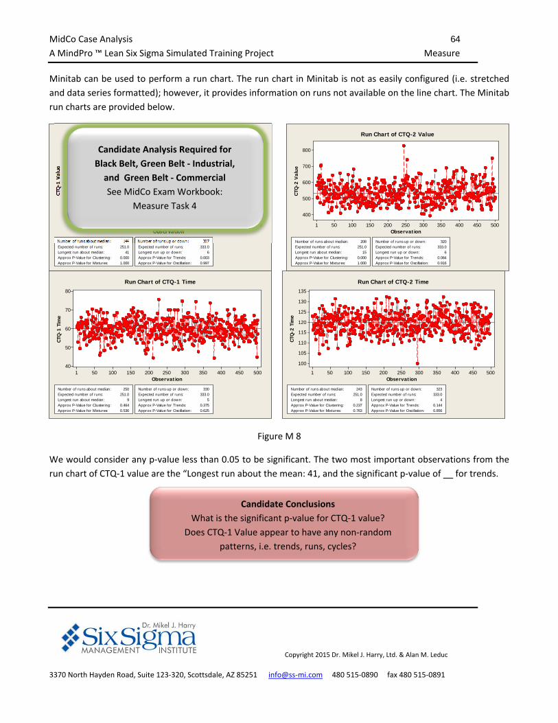
MidCo Case Analysis 64
A MindPro ™ Lean Six Sigma Simulated Training Project Measure
Copyright 2015 Dr. Mikel J. Harry, Ltd. & Alan M. Leduc
3370 North Hayden Road, Suite 123‐320, Scottsdale, AZ 85251 info@ss‐mi.com 480 515‐0890 fax 480 515‐0891
Minitab can be used to perform a run chart. The run chart in Minitab is not as easily configured (i.e. stretched
and data series formatted); however, it provides information on runs not available on the line chart. The Minitab
run charts are provided below.
500450400350300250200150100501
120
100
80
60
40
20
Observation
CTQ
-1 V
alue
Number of runs about median: 144Expected number of runs: 251.0Longest run about median: 41Approx P-Value for Clustering: 0.000Approx P-Value for Mixtures: 1.000
Number of runs up or down: 307Expected number of runs: 333.0Longest run up or down: 6Approx P-Value for Trends: 0.003Approx P-Value for Oscillation: 0.997
Run Chart of CTQ-1 Value
500450400350300250200150100501
800
700
600
500
400
Observation
CTQ
-2 V
alue
Number of runs about median: 208Expected number of runs: 251.0Longest run about median: 15Approx P-Value for Clustering: 0.000Approx P-Value for Mixtures: 1.000
Number of runs up or down: 320Expected number of runs: 333.0Longest run up or down: 6Approx P-Value for Trends: 0.084Approx P-Value for Oscillation: 0.916
Run Chart of CTQ-2 Value
500450400350300250200150100501
80
70
60
50
40
Observation
CTQ
-1 T
ime
Number of runs about median: 250Expected number of runs: 251.0Longest run about median: 9Approx P-Value for Clustering: 0.464Approx P-Value for Mixtures: 0.536
Number of runs up or down: 330Expected number of runs: 333.0Longest run up or down: 5Approx P-Value for Trends: 0.375Approx P-Value for Oscillation: 0.625
Run Chart of CTQ-1 Time
500450400350300250200150100501
135
130
125
120
115
110
105
100
Observation
CTQ
-2 T
ime
Number of runs about median: 243Expected number of runs: 251.0Longest run about median: 8Approx P-Value for Clustering: 0.237Approx P-Value for Mixtures: 0.763
Number of runs up or down: 323Expected number of runs: 333.0Longest run up or down: 4Approx P-Value for Trends: 0.144Approx P-Value for Oscillation: 0.856
Run Chart of CTQ-2 Time
Figure M 8
We would consider any p‐value less than 0.05 to be significant. The two most important observations from the
run chart of CTQ‐1 value are the “Longest run about the mean: 41, and the significant p‐value of __ for trends.
Candidate Analysis Required for
Black Belt, Green Belt ‐ Industrial,
and Green Belt ‐ Commercial
See MidCo Exam Workbook:
Measure Task 4
Candidate Conclusions
What is the significant p‐value for CTQ‐1 value?
Does CTQ‐1 Value appear to have any non‐random
patterns, i.e. trends, runs, cycles?
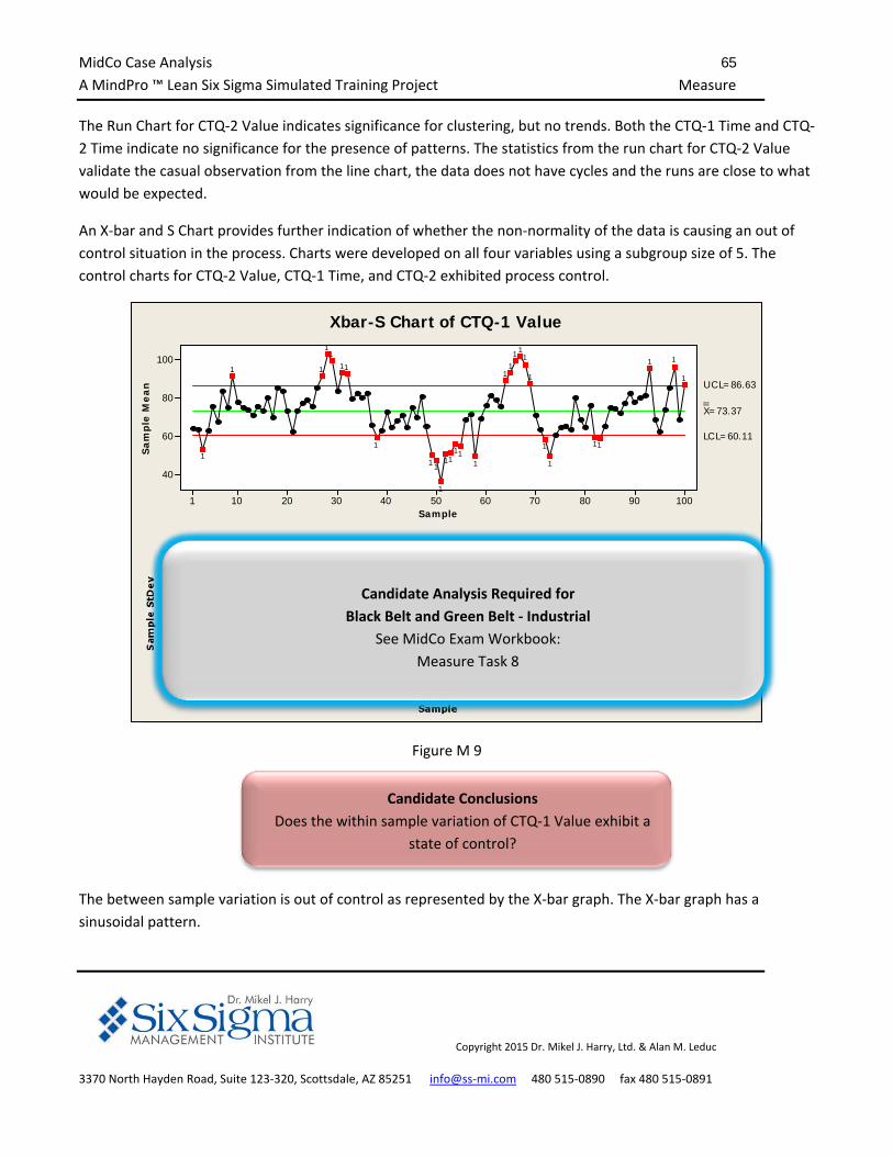
MidCo Case Analysis 65
A MindPro ™ Lean Six Sigma Simulated Training Project Measure
Copyright 2015 Dr. Mikel J. Harry, Ltd. & Alan M. Leduc
3370 North Hayden Road, Suite 123‐320, Scottsdale, AZ 85251 info@ss‐mi.com 480 515‐0890 fax 480 515‐0891
The Run Chart for CTQ‐2 Value indicates significance for clustering, but no trends. Both the CTQ‐1 Time and CTQ‐
2 Time indicate no significance for the presence of patterns. The statistics from the run chart for CTQ‐2 Value
validate the casual observation from the line chart, the data does not have cycles and the runs are close to what
would be expected.
An X‐bar and S Chart provides further indication of whether the non‐normality of the data is causing an out of
control situation in the process. Charts were developed on all four variables using a subgroup size of 5. The
control charts for CTQ‐2 Value, CTQ‐1 Time, and CTQ‐2 exhibited process control.
Sample
Sa
mp
le M
ea
n
1009080706050403020101
100
80
60
40
__X=73.37
UC L=86.63
LC L=60.11
Sample
Sa
mp
le S
tDe
v
1009080706050403020101
20
15
10
5
0
_S=9.29
UC L=19.41
LC L=0
1
11
11
1
1
1
111
11
111
11
1
11
1
11
11
11
1
1
Xbar-S Chart of CTQ-1 Value
Figure M 9
The between sample variation is out of control as represented by the X‐bar graph. The X‐bar graph has a
sinusoidal pattern.
Candidate Analysis Required for
Black Belt and Green Belt ‐ Industrial
See MidCo Exam Workbook:
Measure Task 8
Candidate Conclusions
Does the within sample variation of CTQ‐1 Value exhibit a
state of control?
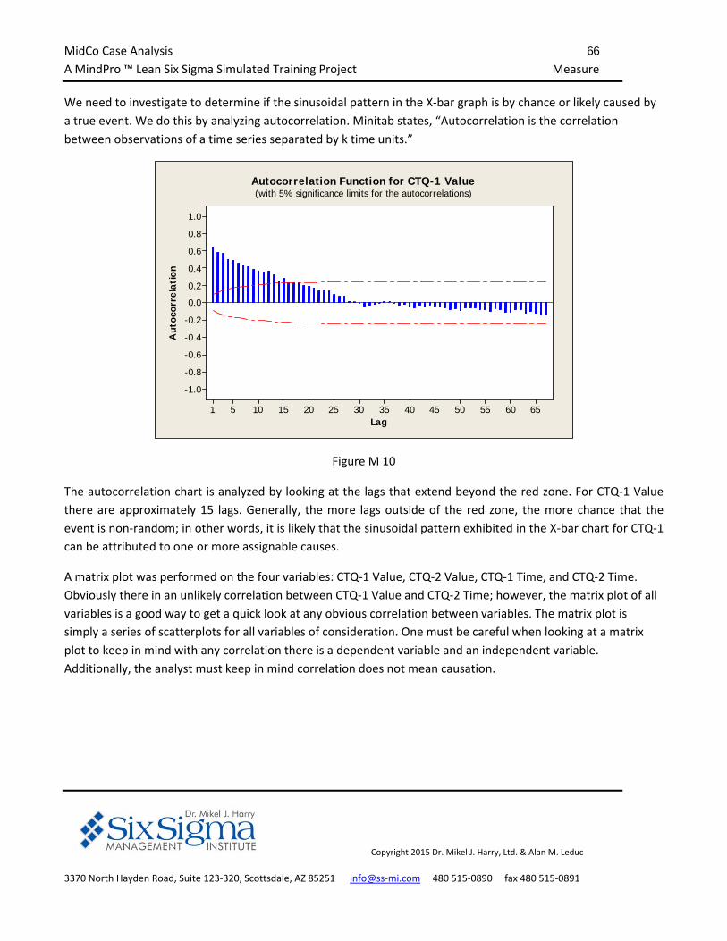
MidCo Case Analysis 66
A MindPro ™ Lean Six Sigma Simulated Training Project Measure
Copyright 2015 Dr. Mikel J. Harry, Ltd. & Alan M. Leduc
3370 North Hayden Road, Suite 123‐320, Scottsdale, AZ 85251 info@ss‐mi.com 480 515‐0890 fax 480 515‐0891
We need to investigate to determine if the sinusoidal pattern in the X‐bar graph is by chance or likely caused by
a true event. We do this by analyzing autocorrelation. Minitab states, “Autocorrelation is the correlation
between observations of a time series separated by k time units.”
Lag
Aut
ocor
rela
tion
65605550454035302520151051
1.0
0.8
0.6
0.4
0.2
0.0
-0.2
-0.4
-0.6
-0.8
-1.0
Autocorrelation Function for CTQ-1 Value(with 5% significance limits for the autocorrelations)
Figure M 10
The autocorrelation chart is analyzed by looking at the lags that extend beyond the red zone. For CTQ‐1 Value
there are approximately 15 lags. Generally, the more lags outside of the red zone, the more chance that the
event is non‐random; in other words, it is likely that the sinusoidal pattern exhibited in the X‐bar chart for CTQ‐1
can be attributed to one or more assignable causes.
A matrix plot was performed on the four variables: CTQ‐1 Value, CTQ‐2 Value, CTQ‐1 Time, and CTQ‐2 Time.
Obviously there in an unlikely correlation between CTQ‐1 Value and CTQ‐2 Time; however, the matrix plot of all
variables is a good way to get a quick look at any obvious correlation between variables. The matrix plot is
simply a series of scatterplots for all variables of consideration. One must be careful when looking at a matrix
plot to keep in mind with any correlation there is a dependent variable and an independent variable.
Additionally, the analyst must keep in mind correlation does not mean causation.
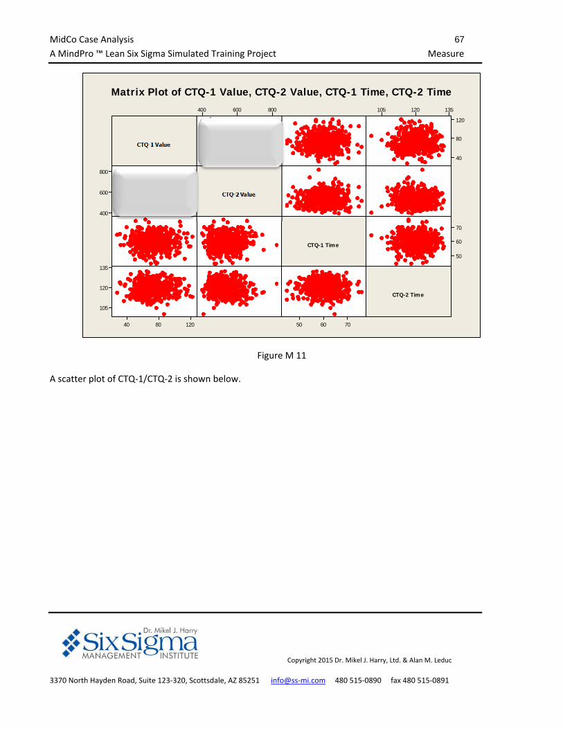
MidCo Case Analysis 67
A MindPro ™ Lean Six Sigma Simulated Training Project Measure
Copyright 2015 Dr. Mikel J. Harry, Ltd. & Alan M. Leduc
3370 North Hayden Road, Suite 123‐320, Scottsdale, AZ 85251 info@ss‐mi.com 480 515‐0890 fax 480 515‐0891
800600400 135120105
120
80
40
800
600
400
70
60
50
1208040
135
120
105
706050
CTQ-1 Value
CTQ-2 Value
CTQ-1 Time
CTQ-2 Time
Matrix Plot of CTQ-1 Value, CTQ-2 Value, CTQ-1 Time, CTQ-2 Time
Figure M 11
A scatter plot of CTQ‐1/CTQ‐2 is shown below.
MidCo Case Analysis 68
A MindPro ™ Lean Six Sigma Simulated Training Project Measure
Copyright 2015 Dr. Mikel J. Harry, Ltd. & Alan M. Leduc
3370 North Hayden Road, Suite 123‐320, Scottsdale, AZ 85251 info@ss‐mi.com 480 515‐0890 fax 480 515‐0891
CTQ-2 Value
CTQ
-1 V
alue
800700600500400
120
100
80
60
40
20
Scatterplot of CTQ-1 Value vs CTQ-2 Value
Figure M 12
A regression analysis was performed using CTQ‐1 as the response variable (Y) and CTQ‐2 as the predictor
variable (X). The regression analysis was significant with a p‐value of 0.000 for the regression equation CTQ‐1
Value = 172 ‐ 0.185 CTQ‐2 Value. The R2 value of 53.6% indicates that 53.6% of the variation in CTQ‐1 is
explained by CTQ‐2. This is an exceptional correlation for cross‐sectional data. It should be noted that the
significance of the regression equation and the high R2 for cross‐sectional data is a prediction and deserves
additional investigation but does not necessarily mean the variation in CTQ‐1 is caused by CTQ‐2.
Candidate Analysis Required for
Black Belt, Green Belt ‐ Industrial, and
Green Belt ‐ Commercial
See MidCo Exam Workbook:
Measure Task 5
Candidate Conclusions
Does there appear to be correlation between CTQ‐1 value
and CTQ‐2 value?
MidCo Case Analysis 69
A MindPro ™ Lean Six Sigma Simulated Training Project Measure
Copyright 2015 Dr. Mikel J. Harry, Ltd. & Alan M. Leduc
3370 North Hayden Road, Suite 123‐320, Scottsdale, AZ 85251 info@ss‐mi.com 480 515‐0890 fax 480 515‐0891
Capability Analysis
Capability Analysis generally is only valid on “in‐control processes.” The process for CTQ‐2 Value was in control
but the process for CTQ‐1 Value was clearly out of control. However, in the Measure Phase it is good to provide
a capability analysis on the current state for all variables that will be considered in the Analyze Phase. Therefore,
a thorough capability analysis was performed on both CTQ‐1 Value and CTQ‐2 Value. A subgroup size of 5 was
used for the capability analysis performed in Minitab. Minitab also provides the option of doing what they call a
“Capability Sixpack.” The “Capability Sixpack” was also performed and follows the chart for capability analysis.
Minitab's Capability Sixpack allows the analyst assess the capability of a process at a glance by combining the
following quality tools into a single display:
Xbar or Individuals charts to determine whether the process is in control. If the process in out of
control, the capability indices are invalid. While the X‐bar and R Charts are included in the Capability
Sixpack, it might be desirable to create them individually.
R, S, or MR chart to track the variation in the data and assesses whether the process variation is
acceptable.
A run chart to look for evidence of patterns in the data.
Probability plot to verify that a chosen distribution fits the data.
Capability histogram and capability plot to visually compare the distribution of data from the
process to the specification spread. It also includes capability statistics to assess capability of the
process quantitatively.
MidCo Case Analysis 70
A MindPro ™ Lean Six Sigma Simulated Training Project Measure
Copyright 2015 Dr. Mikel J. Harry, Ltd. & Alan M. Leduc
3370 North Hayden Road, Suite 123‐320, Scottsdale, AZ 85251 info@ss‐mi.com 480 515‐0890 fax 480 515‐0891
1201059075604530
LSL USLProcess Data
Sample N 500StDev (Within) 9.88251StDev (O v erall) 15.84360
LSL 45.00000Target *USL 115.00000Sample Mean 73.37280
Potential (Within) C apability
C C pk 1.18
O v erall C apability
Pp 0.74PPL 0.60PPU 0.88Ppk
C p
0.60C pm *
1.18C PL 0.96C PU 1.40C pk 0.96
O bserv ed PerformancePPM < LSL 28000.00PPM > USL 10000.00PPM Total 38000.00
Exp. Within PerformancePPM < LSL 2045.80PPM > USL 12.64PPM Total 2058.45
Exp. O v erall PerformancePPM < LSL 36662.30PPM > USL 4302.23PPM Total 40964.53
WithinOverall
Process Capability of CTQ-1 Value
Figure M 13
Candidate Analysis Required for
Black Belt, Green Belt ‐ Industrial, and Green Belt ‐ Commercial
See MidCo Exam Workbook:
Measure Task 6
Candidate Conclusions
What is the short‐term (within) capability (Cp)? What is
the short term (within) Standard Deviation? What is the
long term (overall) capability (Ppk)? What is the long term
(overall) standard deviation? What is the process mean?
What is the process target? What is the offset between
the mean and the target? What portion of the semi‐
tolerance zone id consumed by the offset? What is the
value of the constant K. (Hint: See equations below)? How
does the short term standard deviation compare to the
long term standard deviation? What do you think causes
this difference? Is there a centering problem? Is there a
spread or variation problem? Is spread or centering the
biggest problem?
MidCo Case Analysis 71
A MindPro ™ Lean Six Sigma Simulated Training Project Measure
Copyright 2015 Dr. Mikel J. Harry, Ltd. & Alan M. Leduc
3370 North Hayden Road, Suite 123‐320, Scottsdale, AZ 85251 info@ss‐mi.com 480 515‐0890 fax 480 515‐0891
9181716151413121111
100
75
50Sam
ple
Mea
n
__X=73.37
UCL=86.63
LCL=60.11
9181716151413121111
40
20
0
Sam
ple
Ran
ge
_R=22.99
UCL=48.61
LCL=0
10095908580
100
75
50
Sample
Valu
es
1201059075604530
LSL USL
LSL 45USL 115
Specifications
120906030
Within
O v erall
Specs
StDev 9.88251C p 1.18C pk 0.96
WithinStDev 15.8357Pp 0.74Ppk 0.6C pm *
O v erall
1
11
11
11
1
111
11
111
11
1
11
1
111
1
11
1
Process Capability Sixpack of CTQ-1 ValueXbar Chart
R Chart
Last 25 Subgroups
Capability Histogram
Normal Prob PlotA D: 1.032, P: 0.010
Capability Plot
Figure M 14
To help understand the data it will be helpful to clarify some terms:
Short Term Capability may also be called within capability or potential capability and represents the
capability of the process if no assignable causes were present.
Long Term Capability may also be called overall capability or sustainable capability.
3Cp = Z = sigma short term
Candidate Analysis Required for
Black Belt and Green Belt ‐ Industrial
See MidCo Exam Workbook:
Measure Task 7
Candidate Conclusions
Is the process mean in statistical control?
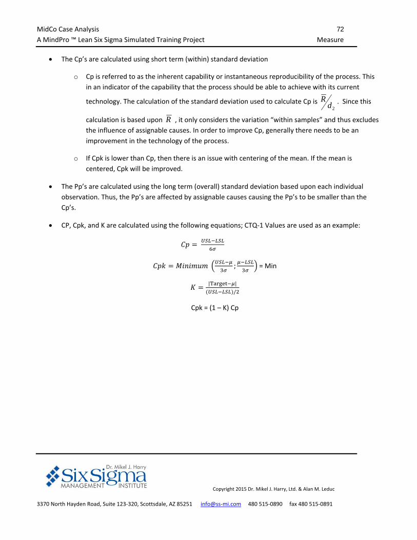
MidCo Case Analysis 72
A MindPro ™ Lean Six Sigma Simulated Training Project Measure
Copyright 2015 Dr. Mikel J. Harry, Ltd. & Alan M. Leduc
3370 North Hayden Road, Suite 123‐320, Scottsdale, AZ 85251 info@ss‐mi.com 480 515‐0890 fax 480 515‐0891
The Cp’s are calculated using short term (within) standard deviation
o Cp is referred to as the inherent capability or instantaneous reproducibility of the process. This
in an indicator of the capability that the process should be able to achieve with its current
technology. The calculation of the standard deviation used to calculate Cp is 2d
R . Since this
calculation is based upon R , it only considers the variation “within samples” and thus excludes
the influence of assignable causes. In order to improve Cp, generally there needs to be an
improvement in the technology of the process.
o If Cpk is lower than Cp, then there is an issue with centering of the mean. If the mean is
centered, Cpk will be improved.
The Pp’s are calculated using the long term (overall) standard deviation based upon each individual
observation. Thus, the Pp’s are affected by assignable causes causing the Pp’s to be smaller than the
Cp’s.
CP, Cpk, and K are calculated using the following equations; CTQ‐1 Values are used as an example:
; = Min
| |
/
Cpk = (1 – K) Cp
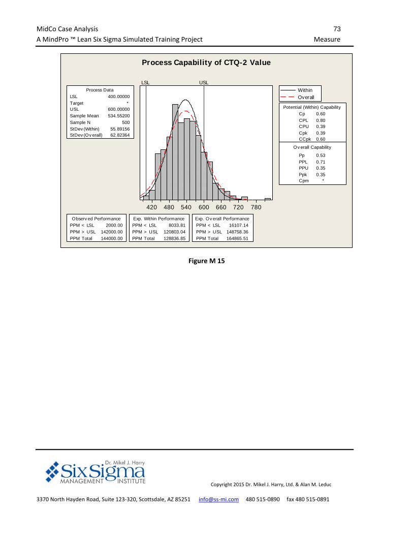
MidCo Case Analysis 73
A MindPro ™ Lean Six Sigma Simulated Training Project Measure
Copyright 2015 Dr. Mikel J. Harry, Ltd. & Alan M. Leduc
3370 North Hayden Road, Suite 123‐320, Scottsdale, AZ 85251 info@ss‐mi.com 480 515‐0890 fax 480 515‐0891
780720660600540480420
LSL USLProcess Data
Sample N 500StDev (Within) 55.89156StDev (O v erall) 62.82364
LSL 400.00000Target *USL 600.00000Sample Mean 534.55200
Potential (Within) C apability
C C pk 0.60
O v erall C apability
Pp 0.53PPL 0.71PPU 0.35Ppk
C p
0.35C pm *
0.60C PL 0.80C PU 0.39C pk 0.39
O bserv ed PerformancePPM < LSL 2000.00PPM > USL 142000.00PPM Total 144000.00
Exp. Within PerformancePPM < LSL 8033.81PPM > USL 120803.04PPM Total 128836.85
Exp. O v erall PerformancePPM < LSL 16107.14PPM > USL 148758.36PPM Total 164865.51
WithinOverall
Process Capability of CTQ-2 Value
Figure M 15
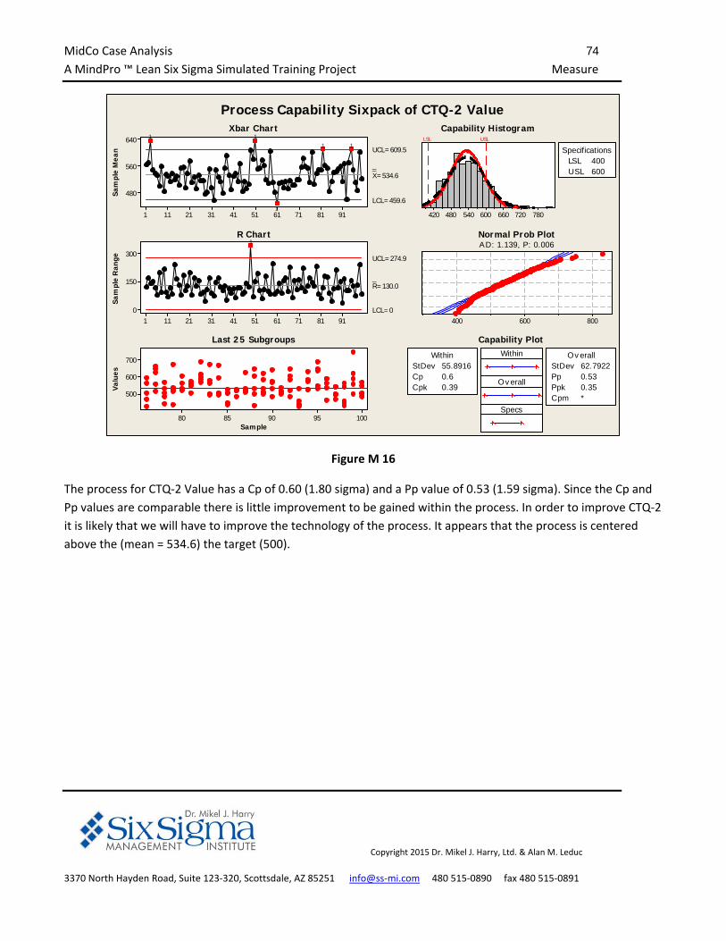
MidCo Case Analysis 74
A MindPro ™ Lean Six Sigma Simulated Training Project Measure
Copyright 2015 Dr. Mikel J. Harry, Ltd. & Alan M. Leduc
3370 North Hayden Road, Suite 123‐320, Scottsdale, AZ 85251 info@ss‐mi.com 480 515‐0890 fax 480 515‐0891
9181716151413121111
640
560
480Sam
ple
Mea
n
__X=534.6
UCL=609.5
LCL=459.6
9181716151413121111
300
150
0
Sam
ple
Ran
ge
_R=130.0
UCL=274.9
LCL=0
10095908580
700
600
500
Sample
Valu
es
780720660600540480420
LSL USL
LSL 400USL 600
Specifications
800600400
Within
O v erall
Specs
StDev 55.8916C p 0.6C pk 0.39
WithinStDev 62.7922Pp 0.53Ppk 0.35C pm *
O v erall
11
1
11
1
Process Capability Sixpack of CTQ-2 ValueXbar Chart
R Chart
Last 25 Subgroups
Capability Histogram
Normal Prob PlotA D: 1.139, P: 0.006
Capability Plot
Figure M 16
The process for CTQ‐2 Value has a Cp of 0.60 (1.80 sigma) and a Pp value of 0.53 (1.59 sigma). Since the Cp and
Pp values are comparable there is little improvement to be gained within the process. In order to improve CTQ‐2
it is likely that we will have to improve the technology of the process. It appears that the process is centered
above the (mean = 534.6) the target (500).
MidCo Case Analysis 75
A MindPro ™ Lean Six Sigma Simulated Training Project Measure
Copyright 2015 Dr. Mikel J. Harry, Ltd. & Alan M. Leduc
3370 North Hayden Road, Suite 123‐320, Scottsdale, AZ 85251 info@ss‐mi.com 480 515‐0890 fax 480 515‐0891
ANOVA of Subgroups
The X‐bar chart plotted subgroups of 5 with several of these subgroups plotting outside the control limits.
Another tool for analyzing the difference in subgroups in Analysis of Variance (ANOVA). A one‐way ANOVA was
performed with CTQ‐1 Value as the response and subgroups as the factor to be analyzed with the results
provided below:
One‐way ANOVA: CTQ‐1 Value versus Subgroup
Source DF SS MS F P
Subgroup 99 86116.6 869.9 8.92 0.000
Error 400 39016.8 97.5
Total 499 125133.4
Candidate Analysis Required for
Black Belt and Green Belt ‐ Industrial
See MidCo Exam Workbook:
Measure Task 9
Candidate Conclusions
What is the F‐value? At what level would the F‐value be
statistically significant? What percent of the total variation
can be explained by subgroup‐to‐subgroup variation? Is
there a need to focus on long term capability (non‐random
pattern issues; black noise)? Is there a need to focus on
short term capability (within variation issues)? What is
more important overall variation or within variation
issues? How does total (overall) standard deviation
compare to short term (within) standard deviation?
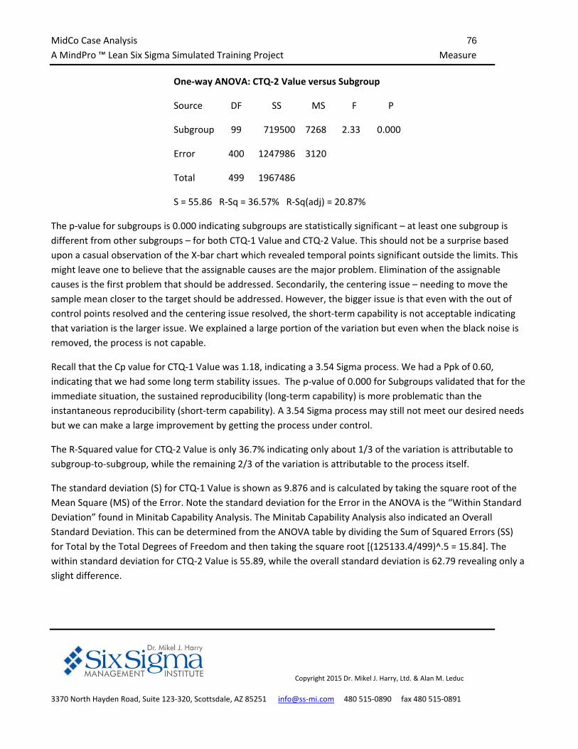
MidCo Case Analysis 76
A MindPro ™ Lean Six Sigma Simulated Training Project Measure
Copyright 2015 Dr. Mikel J. Harry, Ltd. & Alan M. Leduc
3370 North Hayden Road, Suite 123‐320, Scottsdale, AZ 85251 info@ss‐mi.com 480 515‐0890 fax 480 515‐0891
One‐way ANOVA: CTQ‐2 Value versus Subgroup
Source DF SS MS F P
Subgroup 99 719500 7268 2.33 0.000
Error 400 1247986 3120
Total 499 1967486
S = 55.86 R‐Sq = 36.57% R‐Sq(adj) = 20.87%
The p‐value for subgroups is 0.000 indicating subgroups are statistically significant – at least one subgroup is
different from other subgroups – for both CTQ‐1 Value and CTQ‐2 Value. This should not be a surprise based
upon a casual observation of the X‐bar chart which revealed temporal points significant outside the limits. This
might leave one to believe that the assignable causes are the major problem. Elimination of the assignable
causes is the first problem that should be addressed. Secondarily, the centering issue – needing to move the
sample mean closer to the target should be addressed. However, the bigger issue is that even with the out of
control points resolved and the centering issue resolved, the short‐term capability is not acceptable indicating
that variation is the larger issue. We explained a large portion of the variation but even when the black noise is
removed, the process is not capable.
Recall that the Cp value for CTQ‐1 Value was 1.18, indicating a 3.54 Sigma process. We had a Ppk of 0.60,
indicating that we had some long term stability issues. The p‐value of 0.000 for Subgroups validated that for the
immediate situation, the sustained reproducibility (long‐term capability) is more problematic than the
instantaneous reproducibility (short‐term capability). A 3.54 Sigma process may still not meet our desired needs
but we can make a large improvement by getting the process under control.
The R‐Squared value for CTQ‐2 Value is only 36.7% indicating only about 1/3 of the variation is attributable to
subgroup‐to‐subgroup, while the remaining 2/3 of the variation is attributable to the process itself.
The standard deviation (S) for CTQ‐1 Value is shown as 9.876 and is calculated by taking the square root of the
Mean Square (MS) of the Error. Note the standard deviation for the Error in the ANOVA is the “Within Standard
Deviation” found in Minitab Capability Analysis. The Minitab Capability Analysis also indicated an Overall
Standard Deviation. This can be determined from the ANOVA table by dividing the Sum of Squared Errors (SS)
for Total by the Total Degrees of Freedom and then taking the square root [(125133.4/499)^.5 = 15.84]. The
within standard deviation for CTQ‐2 Value is 55.89, while the overall standard deviation is 62.79 revealing only a
slight difference.
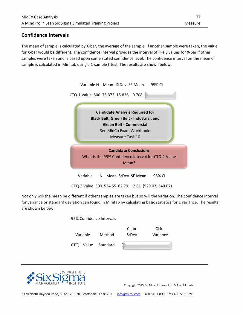
MidCo Case Analysis 77
A MindPro ™ Lean Six Sigma Simulated Training Project Measure
Copyright 2015 Dr. Mikel J. Harry, Ltd. & Alan M. Leduc
3370 North Hayden Road, Suite 123‐320, Scottsdale, AZ 85251 info@ss‐mi.com 480 515‐0890 fax 480 515‐0891
Confidence Intervals
The mean of sample is calculated by X‐bar, the average of the sample. If another sample were taken, the value
for X‐bar would be different. The confidence interval provides the interval of likely values for X‐bar if other
samples were taken and is based upon some stated confidence level. The confidence interval on the mean of
sample is calculated in Minitab using a 1‐sample t‐test. The results are shown below:
Variable N Mean StDev SE Mean 95% CI
CTQ‐1 Value 500 73.373 15.836 0.708 (71.981, 74.764)
Variable N Mean StDev SE Mean 95% CI
CTQ‐2 Value 500 534.55 62.79 2.81 (529.03, 540.07)
Not only will the mean be different if other samples are taken but so will the variation. The confidence interval
for variance or standard deviation can found in Minitab by calculating basic statistics for 1 variance. The results
are shown below:
95% Confidence Intervals
Variable Method
CI for
StDev
CI for
Variance
CTQ‐1 Value Standard (14.9, 16.9) (222, 285)
Candidate Analysis Required for
Black Belt, Green Belt ‐ Industrial, and
Green Belt ‐ Commercial
See MidCo Exam Workbook:
Measure Task 10
Candidate Conclusions
What is the 95% Confidence Interval for CTQ‐1 Value
Mean?
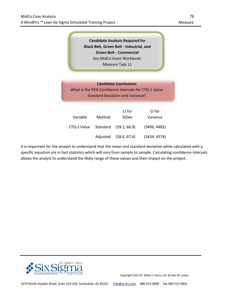
MidCo Case Analysis 78
A MindPro ™ Lean Six Sigma Simulated Training Project Measure
Copyright 2015 Dr. Mikel J. Harry, Ltd. & Alan M. Leduc
3370 North Hayden Road, Suite 123‐320, Scottsdale, AZ 85251 info@ss‐mi.com 480 515‐0890 fax 480 515‐0891
Variable Method
CI for
StDev
CI for
Variance
CTQ‐2 Value Standard (59.1, 66.9) (3496, 4482)
Adjusted (58.6, 67.6) (3434, 4574)
It is important for the analyst to understand that the mean and standard deviation while calculated with a
specific equation are in fact statistics which will vary from sample to sample. Calculating confidence intervals
allows the analyst to understand the likely range of these values and their impact on the project.
Candidate Analysis Required for
Black Belt, Green Belt ‐ Industrial, and
Green Belt ‐ Commercial
See MidCo Exam Workbook:
Measure Task 11
Candidate Conclusions
What is the 95% Confidence Intervals for CTQ‐1 Value
Standard Deviation and Variance?
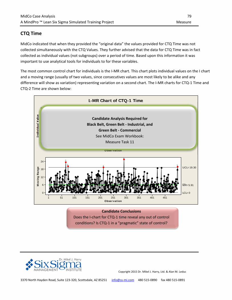
MidCo Case Analysis 79
A MindPro ™ Lean Six Sigma Simulated Training Project Measure
Copyright 2015 Dr. Mikel J. Harry, Ltd. & Alan M. Leduc
3370 North Hayden Road, Suite 123‐320, Scottsdale, AZ 85251 info@ss‐mi.com 480 515‐0890 fax 480 515‐0891
CTQ Time
MidCo indicated that when they provided the “original data” the values provided for CTQ Time was not
collected simultaneously with the CTQ Values. They further advised that the data for CTQ Time was in fact
collected as individual values (not subgroups) over a period of time. Based upon this information it was
important to use analytical tools for individuals to for these variables.
The most common control chart for individuals is the I‐MR chart. This chart plots individual values on the I chart
and a moving range (usually of two values, since consecutives values are most likely to be alike and any
difference will show as variation) representing variation on a second chart. The I‐MR charts for CTQ‐1 Time and
CTQ‐2 Time are shown below:
451401351301251201151101511
80
70
60
50
40
Observation
Ind
ivid
ua
l V
alu
e
_X=59.87
UC L=75.58
LC L=44.16
451401351301251201151101511
24
18
12
6
0
Observation
Mo
vin
g R
an
ge
__MR=5.91
UC L=19.30
LC L=0
1
1
1
11
1
I-MR Chart of CTQ-1 Time
Candidate Analysis Required for
Black Belt, Green Belt ‐ Industrial, and
Green Belt ‐ Commercial
See MidCo Exam Workbook:
Measure Task 11
Candidate Conclusions
Does the I‐chart for CTQ‐1 time reveal any out of control
conditions? Is CTQ‐1 in a “pragmatic” state of control?
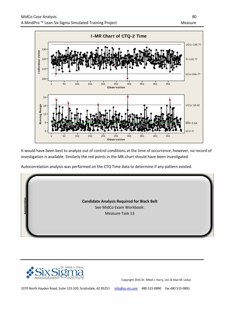
MidCo Case Analysis 80
A MindPro ™ Lean Six Sigma Simulated Training Project Measure
Copyright 2015 Dr. Mikel J. Harry, Ltd. & Alan M. Leduc
3370 North Hayden Road, Suite 123‐320, Scottsdale, AZ 85251 info@ss‐mi.com 480 515‐0890 fax 480 515‐0891
451401351301251201151101511
130
120
110
100
Observation
Ind
ivid
ua
l V
alu
e
_X=119.77
UC L=134.77
LC L=104.77
451401351301251201151101511
24
18
12
6
0
Observation
Mo
vin
g R
an
ge
__MR=5.64
UC L=18.42
LC L=0
1
1
1
1
11
1
I-MR Chart of CTQ-2 Time
It would have been best to analyze out of control conditions at the time of occurrence; however, no record of
investigation is available. Similarly the red points in the MR‐chart should have been investigated
Autocorrelation analysis was performed on the CTQ Time data to determine if any pattern existed.
65605550454035302520151051
1.0
0.8
0.6
0.4
0.2
0.0
-0.2
-0.4
-0.6
-0.8
-1.0
Lag
Aut
ocor
rela
tion
Autocorrelation Function for CTQ-1 Time(with 5% significance limits for the autocorrelations)
65605550454035302520151051
1.0
0.8
0.6
0.4
0.2
0.0
-0.2
-0.4
-0.6
-0.8
-1.0
Lag
Aut
ocor
rela
tion
Autocorrelation Function for CTQ-2 Time(with 5% significance limits for the autocorrelations)
Candidate Analysis Required for Black Belt
See MidCo Exam Workbook:
Measure Task 13
MidCo Case Analysis 81
A MindPro ™ Lean Six Sigma Simulated Training Project Measure
Copyright 2015 Dr. Mikel J. Harry, Ltd. & Alan M. Leduc
3370 North Hayden Road, Suite 123‐320, Scottsdale, AZ 85251 info@ss‐mi.com 480 515‐0890 fax 480 515‐0891
Generally, the more lags outside of the red zone, the more chance that the event is non‐random. This is
consistent with the limited out of control points and stability displayed in the I‐chart.
Evaluation of Test Results
Cross‐tabulation provides one‐way, two‐way, or multi‐way tables containing count data. The optional Chi‐
Square option tests dependence among characteristics in a two‐way classification. This procedure can be used
to test if the probabilities of items being classified for one variable are dependent upon the classification of the
other variable. Unit Test was cross tabulated and the Chi‐square option was employed for CTQ‐1 Test and CTQ‐2
Test with the results shown below:
Tabulated statistics: Unit Test, CTQ-1 Test
Rows: Unit Test Columns: CTQ-1 Test
Fail Pass All
Fail 19 61 80
3.04 76.96 80.00
Pass 0 420 420
15.96 404.04 420.00
All 19 481 500
19.00 481.00 500.00
Cell Contents: Count
Expected count
Pearson Chi-Square = 103.690, DF = 1, P-Value = 0.000
Likelihood Ratio Chi-Square = 73.826, DF = 1, P-Value = 0.000
Candidate Conclusions
Are there any autocorrelation lags outside the confidence
intervals? What is the interpretation of lags outside the
confidence limits?
Candidate Analysis Required for
Black Belt, Green Belt – Industrial, and
Green Belt ‐ Commercial
See MidCo Exam Workbook:
Measure Task 14
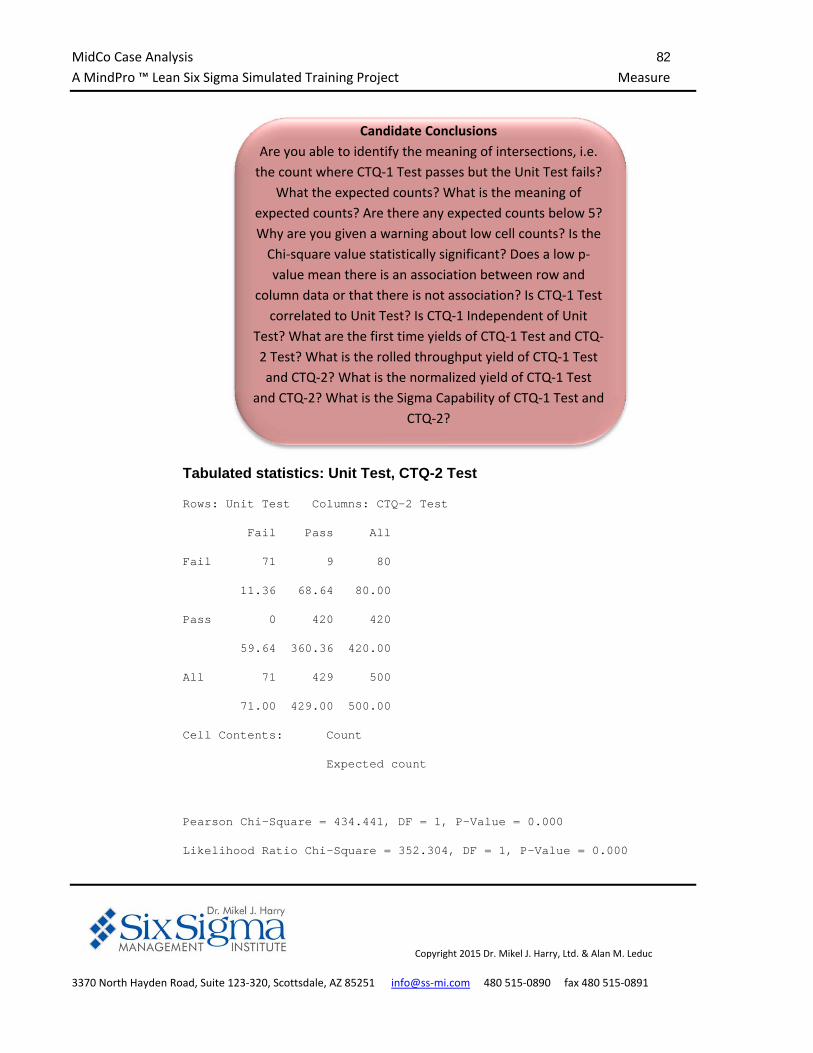
MidCo Case Analysis 82
A MindPro ™ Lean Six Sigma Simulated Training Project Measure
Copyright 2015 Dr. Mikel J. Harry, Ltd. & Alan M. Leduc
3370 North Hayden Road, Suite 123‐320, Scottsdale, AZ 85251 info@ss‐mi.com 480 515‐0890 fax 480 515‐0891
Tabulated statistics: Unit Test, CTQ-2 Test
Rows: Unit Test Columns: CTQ-2 Test
Fail Pass All
Fail 71 9 80
11.36 68.64 80.00
Pass 0 420 420
59.64 360.36 420.00
All 71 429 500
71.00 429.00 500.00
Cell Contents: Count
Expected count
Pearson Chi-Square = 434.441, DF = 1, P-Value = 0.000
Likelihood Ratio Chi-Square = 352.304, DF = 1, P-Value = 0.000
Candidate Conclusions
Are you able to identify the meaning of intersections, i.e.
the count where CTQ‐1 Test passes but the Unit Test fails?
What the expected counts? What is the meaning of
expected counts? Are there any expected counts below 5?
Why are you given a warning about low cell counts? Is the
Chi‐square value statistically significant? Does a low p‐
value mean there is an association between row and
column data or that there is not association? Is CTQ‐1 Test
correlated to Unit Test? Is CTQ‐1 Independent of Unit
Test? What are the first time yields of CTQ‐1 Test and CTQ‐
2 Test? What is the rolled throughput yield of CTQ‐1 Test
and CTQ‐2? What is the normalized yield of CTQ‐1 Test
and CTQ‐2? What is the Sigma Capability of CTQ‐1 Test and
CTQ‐2?
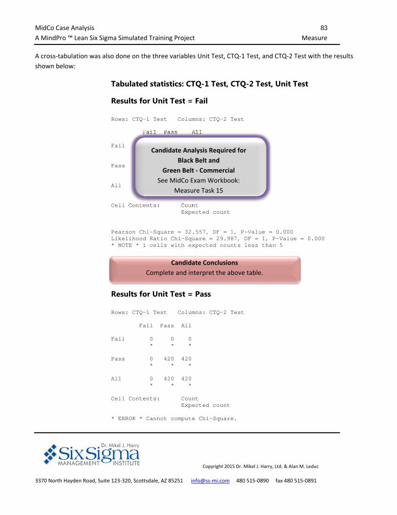
MidCo Case Analysis 83
A MindPro ™ Lean Six Sigma Simulated Training Project Measure
Copyright 2015 Dr. Mikel J. Harry, Ltd. & Alan M. Leduc
3370 North Hayden Road, Suite 123‐320, Scottsdale, AZ 85251 info@ss‐mi.com 480 515‐0890 fax 480 515‐0891
A cross‐tabulation was also done on the three variables Unit Test, CTQ‐1 Test, and CTQ‐2 Test with the results
shown below:
Tabulated statistics: CTQ-1 Test, CTQ-2 Test, Unit Test
Results for Unit Test = Fail Rows: CTQ-1 Test Columns: CTQ-2 Test Fail Pass All Fail 10 9 19 16.86 2.14 19.00 Pass 61 0 61 54.14 6.86 61.00 All 71 9 80 71.00 9.00 80.00 Cell Contents: Count Expected count Pearson Chi-Square = 32.557, DF = 1, P-Value = 0.000 Likelihood Ratio Chi-Square = 29.987, DF = 1, P-Value = 0.000 * NOTE * 1 cells with expected counts less than 5
Results for Unit Test = Pass Rows: CTQ-1 Test Columns: CTQ-2 Test Fail Pass All Fail 0 0 0 * * * Pass 0 420 420 * * * All 0 420 420 * * * Cell Contents: Count Expected count * ERROR * Cannot compute Chi-Square.
Candidate Analysis Required for
Black Belt and
Green Belt ‐ Commercial
See MidCo Exam Workbook:
Measure Task 15
Candidate Conclusions
Complete and interpret the above table.
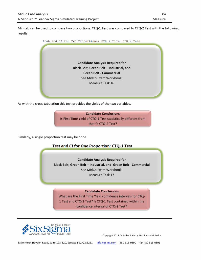
MidCo Case Analysis 84
A MindPro ™ Lean Six Sigma Simulated Training Project Measure
Copyright 2015 Dr. Mikel J. Harry, Ltd. & Alan M. Leduc
3370 North Hayden Road, Suite 123‐320, Scottsdale, AZ 85251 info@ss‐mi.com 480 515‐0890 fax 480 515‐0891
Minitab can be used to compare two proportions. CTQ‐1 Test was compared to CTQ‐2 Test with the following
results.
Test and CI for Two Proportions: CTQ-1 Test, CTQ-2 Test Event = Pass Variable X N Sample p CTQ-1 Test 481 500 0.962000 CTQ-2 Test 429 500 0.858000 Difference = p (CTQ-1 Test) - p (CTQ-2 Test) Estimate for difference: 0.104 95% CI for difference: (0.0691157, 0.138884) Test for difference = 0 (vs not = 0): Z = 5.84 P-Value = 0.000 Fisher's exact test: P-Value = 0.000
As with the cross‐tabulation this test provides the yields of the two variables.
Similarly, a single proportion test may be done.
Test and CI for One Proportion: CTQ-1 Test Event = Pass Variable X N Sample p 95% CI CTQ-1 Test 481 500 0.962000 (0.941293, 0.976969) Variable X N Sample p 95% CI CTQ-2 Test 429 500 0.858000 (0.824289, 0.887403)
Candidate Analysis Required for
Black Belt, Green Belt – Industrial, and
Green Belt ‐ Commercial
See MidCo Exam Workbook:
Measure Task 16
Candidate Conclusions
Is First Time Yield of CTQ‐1 Test statistically different from
that fo CTQ‐2 Test?
Candidate Analysis Required for
Black Belt, Green Belt – Industrial, and Green Belt ‐ Commercial
See MidCo Exam Workbook:
Measure Task 17
Candidate Conclusions
What are the First Time Yield confidence intervals for CTQ‐
1 Test and CTQ‐2 Test? Is CTQ‐1 Test contained within the
confidence interval of CTQ‐2 Test?
MidCo Case Analysis 85
A MindPro ™ Lean Six Sigma Simulated Training Project Measure
Copyright 2015 Dr. Mikel J. Harry, Ltd. & Alan M. Leduc
3370 North Hayden Road, Suite 123‐320, Scottsdale, AZ 85251 info@ss‐mi.com 480 515‐0890 fax 480 515‐0891
The test for two proportions indicated the yields of CTQ‐1 Test and CTQ‐2 Test were different. This can be
verified by looking at the confidence intervals for the two variables
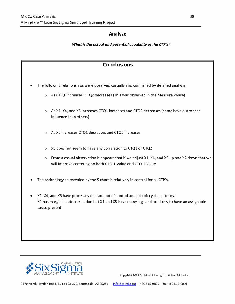
MidCo Case Analysis 86
A MindPro ™ Lean Six Sigma Simulated Training Project
Copyright 2015 Dr. Mikel J. Harry, Ltd. & Alan M. Leduc
3370 North Hayden Road, Suite 123‐320, Scottsdale, AZ 85251 info@ss‐mi.com 480 515‐0890 fax 480 515‐0891
Analyze
What is the actual and potential capability of the CTP’s?
Conclusions
The following relationships were observed casually and confirmed by detailed analysis.
o As CTQ1 increases; CTQ2 decreases (This was observed in the Measure Phase).
o As X1, X4, and X5 increases CTQ1 increases and CTQ2 decreases (some have a stronger
influence than others)
o As X2 increases CTQ1 decreases and CTQ2 increases
o X3 does not seem to have any correlation to CTQ1 or CTQ2
o From a casual observation it appears that if we adjust X1, X4, and X5 up and X2 down that we
will improve centering on both CTQ‐1 Value and CTQ‐2 Value.
The technology as revealed by the S chart is relatively in control for all CTP’s.
X2, X4, and X5 have processes that are out of control and exhibit cyclic patterns.
X2 has marginal autocorrelation but X4 and X5 have many lags and are likely to have an assignable
cause present.
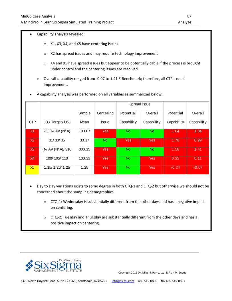
MidCo Case Analysis 87
A MindPro ™ Lean Six Sigma Simulated Training Project Analyze
Copyright 2015 Dr. Mikel J. Harry, Ltd. & Alan M. Leduc
3370 North Hayden Road, Suite 123‐320, Scottsdale, AZ 85251 info@ss‐mi.com 480 515‐0890 fax 480 515‐0891
Capability analysis revealed:
o X1, X3, X4, and X5 have centering issues
o X2 has spread issues and may require technology improvement
o X4 and X5 have spread issues but appear to be potentially cable if the process is brought
under control and the centering issues are resolved.
o Overall capability ranged from ‐0.07 to 1.41 Z‐Benchmark; therefore, all CTP’s need
improvement.
A capability analysis was performed on all variables as summarized below:
CTP LSL/Target/USL
Sample
Mean
Centering
Issue
Spread Issue
Potential
Capability
Overall
Capability
Potential
Capability
Overall
Capability
X1 90/(N/A)/(N/A) 100.07 Yes No No 1.04 1.04
X2 31/33/35 33.17 No Yes Yes 1.76 0.99
X3 (N/A)/(N/A)/310 300.15 Yes No No 1.56 1.41
X4 100/105/110 100.33 Yes No Yes 0.35 0.11
X5 1.15/1.20/1.25 1.25 Yes No Yes -0.24 -0.07
Day to Day variations exists to some degree in both CTQ‐1 and CTQ‐2 but otherwise we should not be
concerned about the sampling demographics.
o CTQ‐1: Wednesday is substantially different from the other days and has a negative impact
on centering.
o CTQ‐2: Tuesday and Thursday are substantially different from the other days and has a
positive impact on centering.
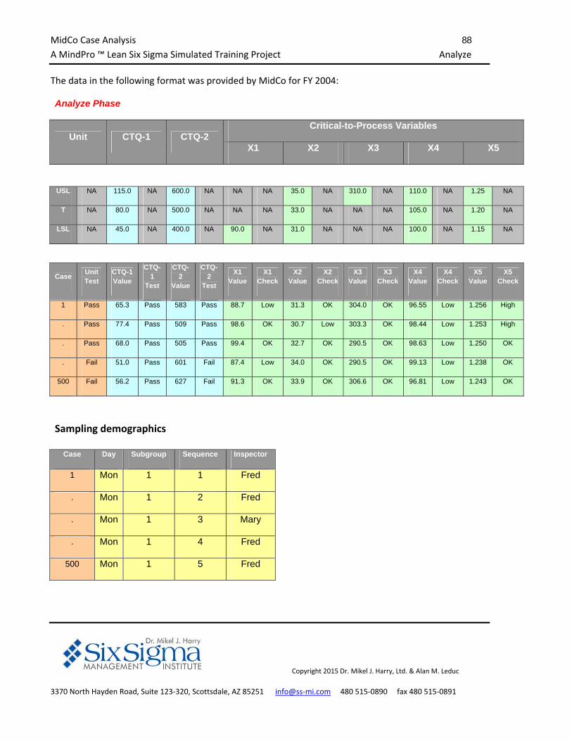
MidCo Case Analysis 88
A MindPro ™ Lean Six Sigma Simulated Training Project Analyze
Copyright 2015 Dr. Mikel J. Harry, Ltd. & Alan M. Leduc
3370 North Hayden Road, Suite 123‐320, Scottsdale, AZ 85251 info@ss‐mi.com 480 515‐0890 fax 480 515‐0891
The data in the following format was provided by MidCo for FY 2004:
Analyze Phase
Unit CTQ-1 CTQ-2 Critical-to-Process Variables
X1 X2 X3 X4 X5
USL NA 115.0 NA 600.0 NA NA NA 35.0 NA 310.0 NA 110.0 NA 1.25 NA
T NA 80.0 NA 500.0 NA NA NA 33.0 NA NA NA 105.0 NA 1.20 NA
LSL NA 45.0 NA 400.0 NA 90.0 NA 31.0 NA NA NA 100.0 NA 1.15 NA
Case Unit Test
CTQ-1 Value
CTQ-1
Test
CTQ-2
Value
CTQ-2
Test
X1 Value
X1 Check
X2 Value
X2 Check
X3 Value
X3 Check
X4 Value
X4 Check
X5 Value
X5 Check
1 Pass 65.3 Pass 583 Pass 88.7 Low 31.3 OK 304.0 OK 96.55 Low 1.256 High
. Pass 77.4 Pass 509 Pass 98.6 OK 30.7 Low 303.3 OK 98.44 Low 1.253 High
. Pass 68.0 Pass 505 Pass 99.4 OK 32.7 OK 290.5 OK 98.63 Low 1.250 OK
. Fail 51.0 Pass 601 Fail 87.4 Low 34.0 OK 290.5 OK 99.13 Low 1.238 OK
500 Fail 56.2 Pass 627 Fail 91.3 OK 33.9 OK 306.6 OK 96.81 Low 1.243 OK
Sampling demographics
Case Day Subgroup Sequence Inspector
1 Mon 1 1 Fred
. Mon 1 2 Fred
. Mon 1 3 Mary
. Mon 1 4 Fred
500 Mon 1 5 Fred
MidCo Case Analysis 89
A MindPro ™ Lean Six Sigma Simulated Training Project Analyze
Copyright 2015 Dr. Mikel J. Harry, Ltd. & Alan M. Leduc
3370 North Hayden Road, Suite 123‐320, Scottsdale, AZ 85251 info@ss‐mi.com 480 515‐0890 fax 480 515‐0891
Overview
The Recognize Phase indicated that we should concentrate on yield as the performance metric to drive Six Sigma
and that our focus should be on the United States facility. In the Define Phase CTQ‐1 and CTQ‐2 were identified
as the most important of the ten CTQ’s. In the Measure Phase, CTQ‐1 and CTQ‐2 was analyzed in terms of its
performance measure including cycle time. In the Analyze Phase, the focus will be on determining the Critical to
Process (CTP) characteristics.
There is a significant amount of analysis required given the amount of data that has been provided. How do we
avoid analysis paralysis – that is analyzing to data ad infinitum? This analysis will systematically analyze
correlation, normality, control, and capability. The analysis will also look at the sampling demographics for
possible issues with inspectors or days of the week.
The Matrix Plot in Minitab provides a quick overview of the data to identify possible correlations.
120
80
40
1.301.251.20
800600400 35.032.530.0 11010090
800
600
400
120
100
80
35.0
32.5
30.0
320
300
280 110
100
90
1208040
1.30
1.25
1.20
12010080 320300280
CTQ-1 Value
CTQ-2 Value
X1 Value
X2 Value
X3 Value
X4 Value
X5 Value
Matrix Plot of CTQ-1 Value, CTQ-2 Value, X1 Value, X2 Value, ...
Candidate Analysis Required for
Black Belt, Green Belt – Industrial, and Green Belt ‐ Commercial
See MidCo Exam Workbook:
Analyze Task 2
MidCo Case Analysis 90
A MindPro ™ Lean Six Sigma Simulated Training Project Analyze
Copyright 2015 Dr. Mikel J. Harry, Ltd. & Alan M. Leduc
3370 North Hayden Road, Suite 123‐320, Scottsdale, AZ 85251 info@ss‐mi.com 480 515‐0890 fax 480 515‐0891
The Matrix Plot reveals the following possible relationships:
As CTQ1-Value increases; CTQ2-Value decreases (This was observed in the Measure Phase).
While not extremely strong, X1, X4, and X5 appear to have a positive correlation with CTQ1-Value.
X1 appears to have a negative correlation with CTQ2-Value.)
The correlation between X4 and CTQ1-Value appears to be a moderate positive correlation that is heteroscedastic (variation is not equal) in nature.
As X2 it appears that CTQ1-Value may decrease while CTQ2-Value may increases. The correlation is not strong.
X3 does not seem to have any correlation to CTQ1-Value and CTQ2-Value
Candidate Analysis Required for
Black Belt, Green Belt – Industrial, and Green Belt ‐ Commercial
See MidCo Exam Workbook:
Analyze Task 2
Candidate Conclusions
What are your conclusions with regard to the Matrix Plot?
No relationship, moderate relationship, strong
relationship? Positive or negative correlation? Does any
heteroscedastic behavior exist?
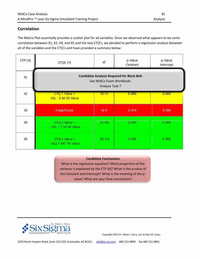
MidCo Case Analysis 91
A MindPro ™ Lean Six Sigma Simulated Training Project Analyze
Copyright 2015 Dr. Mikel J. Harry, Ltd. & Alan M. Leduc
3370 North Hayden Road, Suite 123‐320, Scottsdale, AZ 85251 info@ss‐mi.com 480 515‐0890 fax 480 515‐0891
Correlation
The Matrix Plot essentially provides a scatter plot for all variables. Since we observed what appears to be some
correlation between X1, X2, X4, and X5 and the two CTQ’s, we decided to perform a regression analysis between
all of the variables and the CTQ’s and have provided a summary below:
CTP (X)
CTQ1 (Y)
R2
p-Value Constant
p-Value
Intercept
X1
CTQ-1 Value = - 18.7 + 0.920 X1 Value
31.8% 0.002 0.000
X2
CTQ-1 Value = 191 - 3.56 X2 Value
10.1% 0.000 0.000
X3
Insignificant
N/A
0.474
0.090
X4
CTQ-1 Value = - 181 + 2.54 X4 Value
22.9% 0.000 0.000
X5
CTQ-1 Value = - 612 + 547 X5 Value
52.1% 0.000 0.000
Candidate Analysis Required for Black Belt
See MidCo Exam Workbook:
Analyze Task 7
Candidate Conclusions
What is the regression equation? What proportion of the
variance is explained by the CTP (X)? What is the p‐value of
the Constant and Intercept? What is the meaning of the p‐
value? What are your final conclusions?
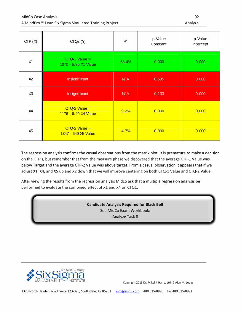
MidCo Case Analysis 92
A MindPro ™ Lean Six Sigma Simulated Training Project Analyze
Copyright 2015 Dr. Mikel J. Harry, Ltd. & Alan M. Leduc
3370 North Hayden Road, Suite 123‐320, Scottsdale, AZ 85251 info@ss‐mi.com 480 515‐0890 fax 480 515‐0891
CTP (X)
CTQ2 (Y)
R2
p-Value Constant
p-Value
Intercept
X1
CTQ-2 Value =
1070 - 5.35 X1 Value
68.4%
0.000
0.000
X2
Insignificant
N/A
0.595
0.000
X3
Insignificant
N/A
0.133
0.000
X4
CTQ-2 Value =
1176 - 6.40 X4 Value
9.2%
0.000
0.000
X5
CTQ-2 Value =
1347 - 649 X5 Value
4.7%
0.000
0.000
The regression analysis confirms the casual observations from the matrix plot. It is premature to make a decision
on the CTP’s, but remember that from the measure phase we discovered that the average CTP‐1 Value was
below Target and the average CTP‐2 Value was above target. From a casual observation it appears that if we
adjust X1, X4, and X5 up and X2 down that we will improve centering on both CTQ‐1 Value and CTQ‐2 Value.
After viewing the results from the regression analysis Midco ask that a multiple regression analysis be
performed to evaluate the combined effect of X1 and X4 on CTQ1.
Candidate Analysis Required for Black Belt
See MidCo Exam Workbook:
Analyze Task 8
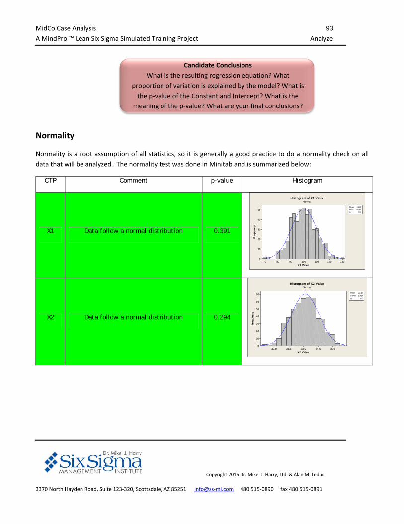
MidCo Case Analysis 93
A MindPro ™ Lean Six Sigma Simulated Training Project Analyze
Copyright 2015 Dr. Mikel J. Harry, Ltd. & Alan M. Leduc
3370 North Hayden Road, Suite 123‐320, Scottsdale, AZ 85251 info@ss‐mi.com 480 515‐0890 fax 480 515‐0891
Normality
Normality is a root assumption of all statistics, so it is generally a good practice to do a normality check on all
data that will be analyzed. The normality test was done in Minitab and is summarized below:
CTP Comment p-value Histogram
X1 Data follow a normal distribution 0.391
130120110100908070
50
40
30
20
10
0
X1 Value
Freq
uenc
y
Mean 100.1StDev 9.708N 500
Histogram of X1 ValueNormal
X2 Data follow a normal distribution 0.294
X2 Value
Freq
uenc
y
36.034.533.031.530.0
70
60
50
40
30
20
10
0
Mean 33.17StDev 1.417N 500
Histogram of X2 ValueNormal
Candidate Conclusions
What is the resulting regression equation? What
proportion of variation is explained by the model? What is
the p‐value of the Constant and Intercept? What is the
meaning of the p‐value? What are your final conclusions?
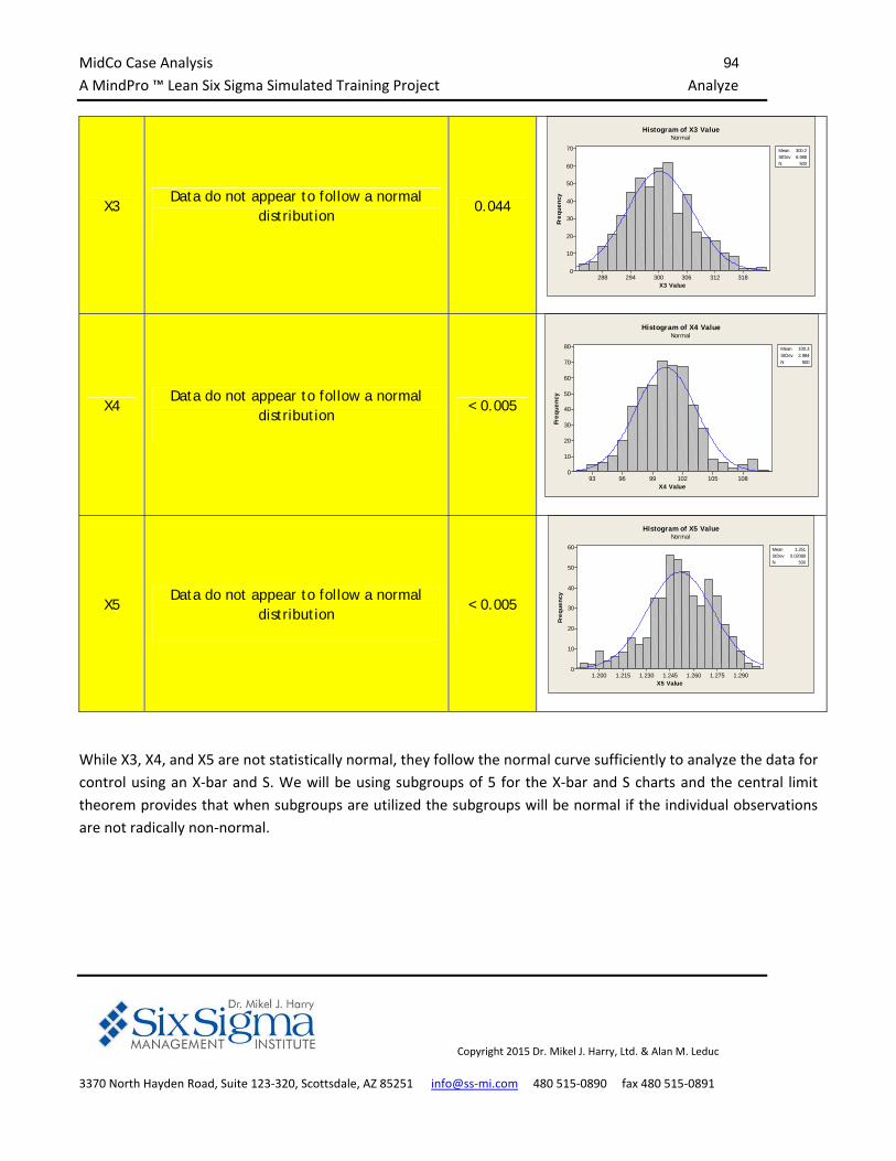
MidCo Case Analysis 94
A MindPro ™ Lean Six Sigma Simulated Training Project Analyze
Copyright 2015 Dr. Mikel J. Harry, Ltd. & Alan M. Leduc
3370 North Hayden Road, Suite 123‐320, Scottsdale, AZ 85251 info@ss‐mi.com 480 515‐0890 fax 480 515‐0891
X3 Data do not appear to follow a normal
distribution 0.044
X3 Value
Freq
uenc
y
318312306300294288
70
60
50
40
30
20
10
0
Mean 300.2StDev 6.988N 500
Histogram of X3 ValueNormal
X4 Data do not appear to follow a normal
distribution < 0.005
X4 Value
Freq
uenc
y
108105102999693
80
70
60
50
40
30
20
10
0
Mean 100.3StDev 2.984N 500
Histogram of X4 ValueNormal
X5 Data do not appear to follow a normal
distribution < 0.005
X5 Value
Freq
uenc
y
1.2901.2751.2601.2451.2301.2151.200
60
50
40
30
20
10
0
Mean 1.251StDev 0.02088N 500
Histogram of X5 ValueNormal
While X3, X4, and X5 are not statistically normal, they follow the normal curve sufficiently to analyze the data for
control using an X‐bar and S. We will be using subgroups of 5 for the X‐bar and S charts and the central limit
theorem provides that when subgroups are utilized the subgroups will be normal if the individual observations
are not radically non‐normal.
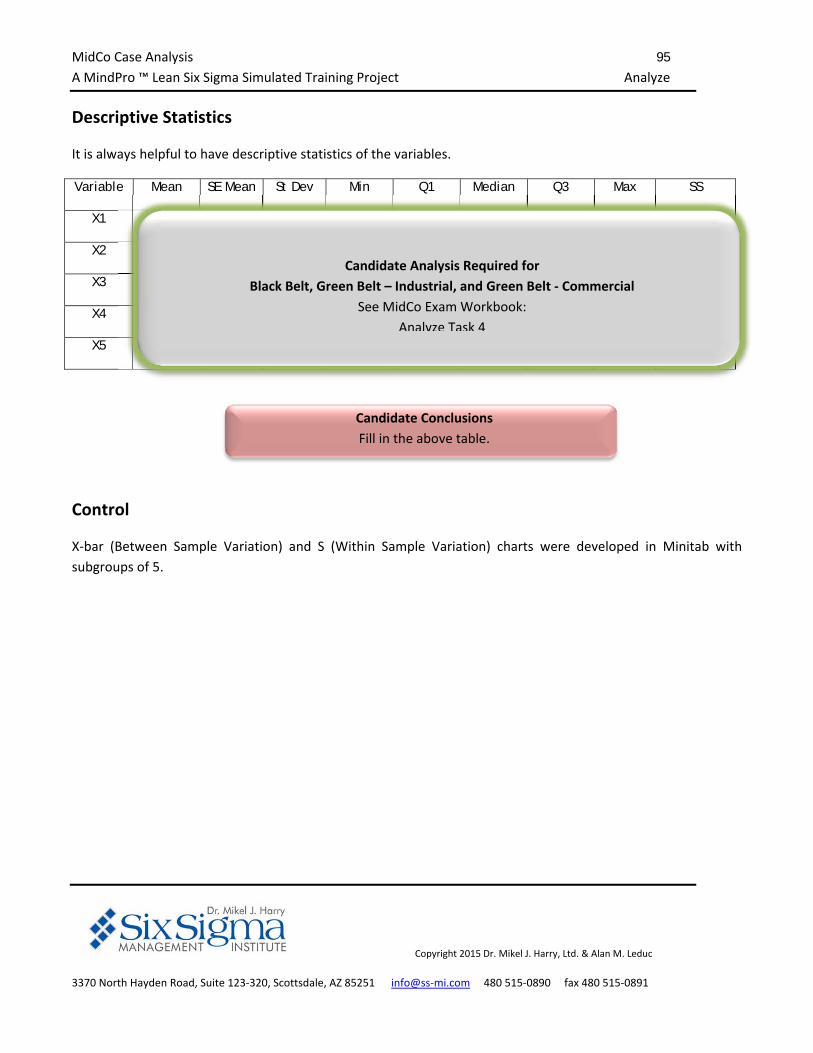
MidCo Case Analysis 95
A MindPro ™ Lean Six Sigma Simulated Training Project Analyze
Copyright 2015 Dr. Mikel J. Harry, Ltd. & Alan M. Leduc
3370 North Hayden Road, Suite 123‐320, Scottsdale, AZ 85251 info@ss‐mi.com 480 515‐0890 fax 480 515‐0891
Descriptive Statistics
It is always helpful to have descriptive statistics of the variables.
Variable Mean SE Mean St Dev Min Q1 Median Q3 Max SS
X1 100.800 0.4340 9.708 68.900 93.000 99.600 106.270 129.400 5,054,634
X2 33.172 0.0634 1.417 29.000 32.100 33.200 34.100 36.900 551,193
X3 300.150 0.3130 6.990 283.500 295.200 299.800 304.850 322.200 45,069,981
X4 100.330 0.1330 2.980 92.480 98.220 100.290 102.090 110.140 5,037,103
X5 1.2514 0.0009 0.0209 1.1900 1.2390 1.2510 1.2680 1.2990 783
Control
X‐bar (Between Sample Variation) and S (Within Sample Variation) charts were developed in Minitab with
subgroups of 5.
Candidate Conclusions
Fill in the above table.
Candidate Analysis Required for
Black Belt, Green Belt – Industrial, and Green Belt ‐ Commercial
See MidCo Exam Workbook:
Analyze Task 4

MidCo Case Analysis 96
A MindPro ™ Lean Six Sigma Simulated Training Project Analyze
Copyright 2015 Dr. Mikel J. Harry, Ltd. & Alan M. Leduc
3370 North Hayden Road, Suite 123‐320, Scottsdale, AZ 85251 info@ss‐mi.com 480 515‐0890 fax 480 515‐0891
9181716151413121111
114
108
102
96
90
Sample
Sa
mp
le M
ea
n
__X=100.08
UC L=113.08
LC L=87.07
9181716151413121111
20
15
10
5
0
Sample
Sa
mp
le S
tDe
v
_S=9.11
UC L=19.04
LC L=0
1
Xbar-S Chart of X1 Value
9181716151413121111
36.0
34.5
33.0
31.5
30.0
Sample
Sa
mp
le M
ea
n
__X=33.172
UC L=34.452
LC L=31.892
9181716151413121111
2.0
1.5
1.0
0.5
0.0
Sample
Sa
mp
le S
tDe
v
_S=0.897
UC L=1.873
LC L=0
1
111
1
11
1
111
1
1
1
11
11
1
1
11
111
1
1
1
1
Xbar-S Chart of X2 Value
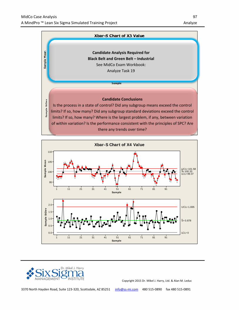
MidCo Case Analysis 97
A MindPro ™ Lean Six Sigma Simulated Training Project Analyze
Copyright 2015 Dr. Mikel J. Harry, Ltd. & Alan M. Leduc
3370 North Hayden Road, Suite 123‐320, Scottsdale, AZ 85251 info@ss‐mi.com 480 515‐0890 fax 480 515‐0891
9181716151413121111
310
305
300
295
290
Sample
Sa
mp
le M
ea
n
__X=300.15
UC L=308.60
LC L=291.70
9181716151413121111
12
9
6
3
0
Sample
Sa
mp
le S
tDe
v
_S=5.92
UC L=12.36
LC L=0
1
1
1
1
1
1
Xbar-S Chart of X3 Value
9181716151413121111
110
105
100
95
Sample
Sa
mp
le M
ea
n
__X=100.33UC L=101.58
LC L=99.07
9181716151413121111
2.0
1.5
1.0
0.5
0.0
Sample
Sa
mp
le S
tDe
v
_S=0.878
UC L=1.835
LC L=0
11
11
1
11
11
11
1
11111
111
1
111
1
111
1
1
1
1
11
1
1
111
1
1
1
1111
1111
1
1
11
1
11
111
11111
1
1
1
Xbar-S Chart of X4 Value
Candidate Conclusions
Is the process in a state of control? Did any subgroup means exceed the control
limits? If so, how many? Did any subgroup standard deviations exceed the control
limits? If so, how many? Where is the largest problem, if any, between variation
of within variation? Is the performance consistent with the principles of SPC? Are
there any trends over time?
Candidate Analysis Required for
Black Belt and Green Belt – Industrial
See MidCo Exam Workbook:
Analyze Task 19
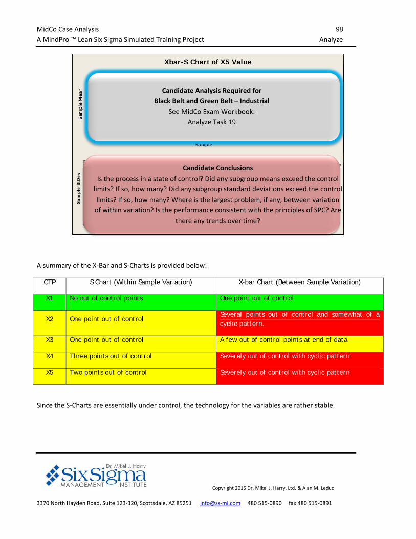
MidCo Case Analysis 98
A MindPro ™ Lean Six Sigma Simulated Training Project Analyze
Copyright 2015 Dr. Mikel J. Harry, Ltd. & Alan M. Leduc
3370 North Hayden Road, Suite 123‐320, Scottsdale, AZ 85251 info@ss‐mi.com 480 515‐0890 fax 480 515‐0891
9181716151413121111
1.28
1.26
1.24
1.22
1.20
Sample
Sa
mp
le M
ea
n
__X=1.2514UC L=1.2591
LC L=1.2436
9181716151413121111
0.012
0.009
0.006
0.003
0.000
Sample
Sa
mp
le S
tDe
v
_S=0.00543
UC L=0.01135
LC L=0
111
1
1111
111
1
1
1
11
111
1
1
1
1
11
1
1111
1
1
11
111
1
1
1
1111
111
1111
11
11
1
1
111
1111
1
11
Xbar-S Chart of X5 Value
A summary of the X‐Bar and S‐Charts is provided below:
CTP S Chart (Within Sample Variation) X-bar Chart (Between Sample Variation)
X1 No out of control points One point out of control
X2 One point out of control Several points out of control and somewhat of a cyclic pattern.
X3 One point out of control A few out of control points at end of data
X4 Three points out of control Severely out of control with cyclic pattern
X5 Two points out of control Severely out of control with cyclic pattern
Since the S‐Charts are essentially under control, the technology for the variables are rather stable.
Candidate Conclusions
Is the process in a state of control? Did any subgroup means exceed the control
limits? If so, how many? Did any subgroup standard deviations exceed the control
limits? If so, how many? Where is the largest problem, if any, between variation
of within variation? Is the performance consistent with the principles of SPC? Are
there any trends over time?
Candidate Analysis Required for
Black Belt and Green Belt – Industrial
See MidCo Exam Workbook:
Analyze Task 19
MidCo Case Analysis 99
A MindPro ™ Lean Six Sigma Simulated Training Project Analyze
Copyright 2015 Dr. Mikel J. Harry, Ltd. & Alan M. Leduc
3370 North Hayden Road, Suite 123‐320, Scottsdale, AZ 85251 info@ss‐mi.com 480 515‐0890 fax 480 515‐0891
Autocorrelation
Autocorrelation for CTQ‐1 Value and CTQ‐1 and CTQ‐2 Time was performed in the measure phase. For CTQ‐1
Value there are approximately 15 lags, indicating a likely sinusoidal pattern exhibited in the X‐bar chart for CTQ‐
1 attributable to one or more assignable causes. CTQ‐1 and CTQ‐2 Time indicated that the data appeared to be
random.
No autocorrelation was performed on CTQ‐2 Value in the Measure Phase as the data appeared to be in control.
Midco ask that this analysis be performed along with the looking at the CTP variables X1 through X5.
65605550454035302520151051
1.0
0.8
0.6
0.4
0.2
0.0
-0.2
-0.4
-0.6
-0.8
-1.0
Lag
Aut
ocor
rela
tion
Autocorrelation Function for CTQ-2 Value(with 5% significance limits for the autocorrelations)
Generally, the more lags outside of the red zone, the more chance that the event is non‐random; with only 5
lags outside the confidence limits it is likely that the data is random as indicated by the evidence of control
determined in the Measure phase.
It is a good idea to check for autocorrelation when a pattern exists in the data as represented by the cycles in
the X‐bar charts of X2, X3, and X5 in order to determine if the pattern is by random chance or likely attributable
to an assignable cause.
Candidate Conclusions
Are any of the lags statistically significant? What is the
meaning of the lags in terms of forecasting?
Candidate Analysis Required for Black Belt
See MidCo Exam Workbook:
Analyze Task 15
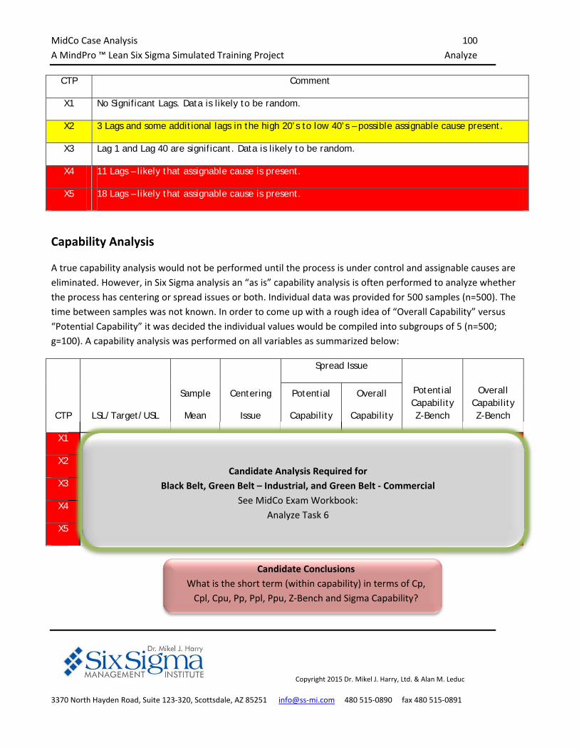
MidCo Case Analysis 100
A MindPro ™ Lean Six Sigma Simulated Training Project Analyze
Copyright 2015 Dr. Mikel J. Harry, Ltd. & Alan M. Leduc
3370 North Hayden Road, Suite 123‐320, Scottsdale, AZ 85251 info@ss‐mi.com 480 515‐0890 fax 480 515‐0891
CTP Comment
X1 No Significant Lags. Data is likely to be random.
X2 3 Lags and some additional lags in the high 20’s to low 40’s – possible assignable cause present.
X3 Lag 1 and Lag 40 are significant. Data is likely to be random.
X4 11 Lags – likely that assignable cause is present.
X5 18 Lags – likely that assignable cause is present.
Capability Analysis
A true capability analysis would not be performed until the process is under control and assignable causes are
eliminated. However, in Six Sigma analysis an “as is” capability analysis is often performed to analyze whether
the process has centering or spread issues or both. Individual data was provided for 500 samples (n=500). The
time between samples was not known. In order to come up with a rough idea of “Overall Capability” versus
“Potential Capability” it was decided the individual values would be compiled into subgroups of 5 (n=500;
g=100). A capability analysis was performed on all variables as summarized below:
CTP LSL/Target/USL
Sample
Mean
Centering
Issue
Spread Issue
Potential Capability Z-Bench
Overall Capability Z-Bench
Potential
Capability
Overall
Capability
X1 90/(N/A)/(N/A) 100.076 Yes Yes Yes 1.04 1.04
X2 31/33/35 33.172 No Yes Yes 1.76 .99
X3 (N/A)/(N/A)/310 300.15 Yes Yes Yes 1.56 1.41
X4 100/105/110 100.33 Yes No Yes 0.35 0.11
X5 1.15/1.20/1.25 1.25 Yes No Yes -0.24 -0.07
Candidate Conclusions
What is the short term (within capability) in terms of Cp,
Cpl, Cpu, Pp, Ppl, Ppu, Z‐Bench and Sigma Capability?
Candidate Analysis Required for
Black Belt, Green Belt – Industrial, and Green Belt ‐ Commercial
See MidCo Exam Workbook:
Analyze Task 6
MidCo Case Analysis 101
A MindPro ™ Lean Six Sigma Simulated Training Project Analyze
Copyright 2015 Dr. Mikel J. Harry, Ltd. & Alan M. Leduc
3370 North Hayden Road, Suite 123‐320, Scottsdale, AZ 85251 info@ss‐mi.com 480 515‐0890 fax 480 515‐0891
Z‐Bench is considered long term Sigma. Short term Sigma is equal to Z‐Bench + 1.5. The Potential (Within)
Capability statistics (Cp, Cpl…) are based off of the estimate for within standard deviation which represents the
variation within subgroups. Overall standard deviation takes into account variation from the entire data set and
looks at the total process variation. The Overall Capability is based on the statistics (Pp, Ppl…). The one sided Cp
is calculated by dividing Z‐Bench by 3.
CTP X1 is in control; however, the process is performing at a very low level. First investigate the
feasibility of increasing the target value. Secondarily investigate decreasing variation as the short term
(within) standard deviation places the mean at only about one standard deviation from the lower
specification limit.
CTP X2 has numerous out of control points on the X‐Bar chart. This is reflected in the difference
between the Potential and Overall Capability. The process is on‐target, so centering is not an issue.
However, with a Potential Capability of only 1.76, variation needs to be reduced and should be
investigated after the process is brought under control.
CTP X3 has several out of control points on the X‐Bar chart. Getting the process in‐control should be the
first priority. Secondarily, investigate the feasibility of decreasing the target value, and thirdly investigate
decreasing variation.
CTP X4 is severely out of control with respect to the X‐Bar chart and has a mean just slightly above the
lower specification limit. The within standard deviation is 0.934 which would result in 10.7 standard
deviations from between specification limits; a little over a Five Sigma short term process, if the out of
control and centering issues can be resolved.
CTP X5 is severely out of control with respect to the X‐Bar chart and has a mean outside the upper
specification limit. The variation is very good if the other issues can be resolved.
MidCo Case Analysis 102
A MindPro ™ Lean Six Sigma Simulated Training Project Analyze
Copyright 2015 Dr. Mikel J. Harry, Ltd. & Alan M. Leduc
3370 North Hayden Road, Suite 123‐320, Scottsdale, AZ 85251 info@ss‐mi.com 480 515‐0890 fax 480 515‐0891
Analysis of Sampling Demographics
Four variables are available for analysis in the sampling demographics: Day; Subgroup; Sequence; Inspector.
MaryFredBill
80
75
70
65
60
Inspector
CTQ
-1 V
alue
FriMonThrTue
Wed
Day
Multi-Vari Chart for CTQ-1 Value by Day - Inspector
Day
CTQ
-1 V
alue
WedTueThrMonFri
80
75
70
65
60
InspectorBill
FredMary
Multi-Vari Chart for CTQ-1 Value by Inspector - Day
MaryFredBill
560
550
540
530
520
Inspector
CTQ
-2 V
alue
FriMonThrTue
Wed
Day
Multi-Vari Chart for CTQ-2 Value by Day - Inspector
Day
CTQ
-2 V
alue
WedTueThrMonFri
560
550
540
530
520
InspectorBill
FredMary
Multi-Vari Chart for CTQ-2 Value by Inspector - Day
Candidate Analysis Required for
Black Belt, Green Belt – Industrial, and Green Belt ‐ Commercial
See MidCo Exam Workbook:
Analyze Task 3
Candidate Conclusions
Interpret the Multi‐vari Charts. Hows does inspector to
inspector variation compare to the day to day variation?
How does the within inspector variation compare to the
between inspector variation? How does the within day
variation compare to between day variation? What
inspectors and days have the largest influence, if any?
Candidate Analysis Required for
Black Belt, Green Belt – Industrial, and Green Belt ‐ Commercial
See MidCo Exam Workbook:
Analyze Task 3
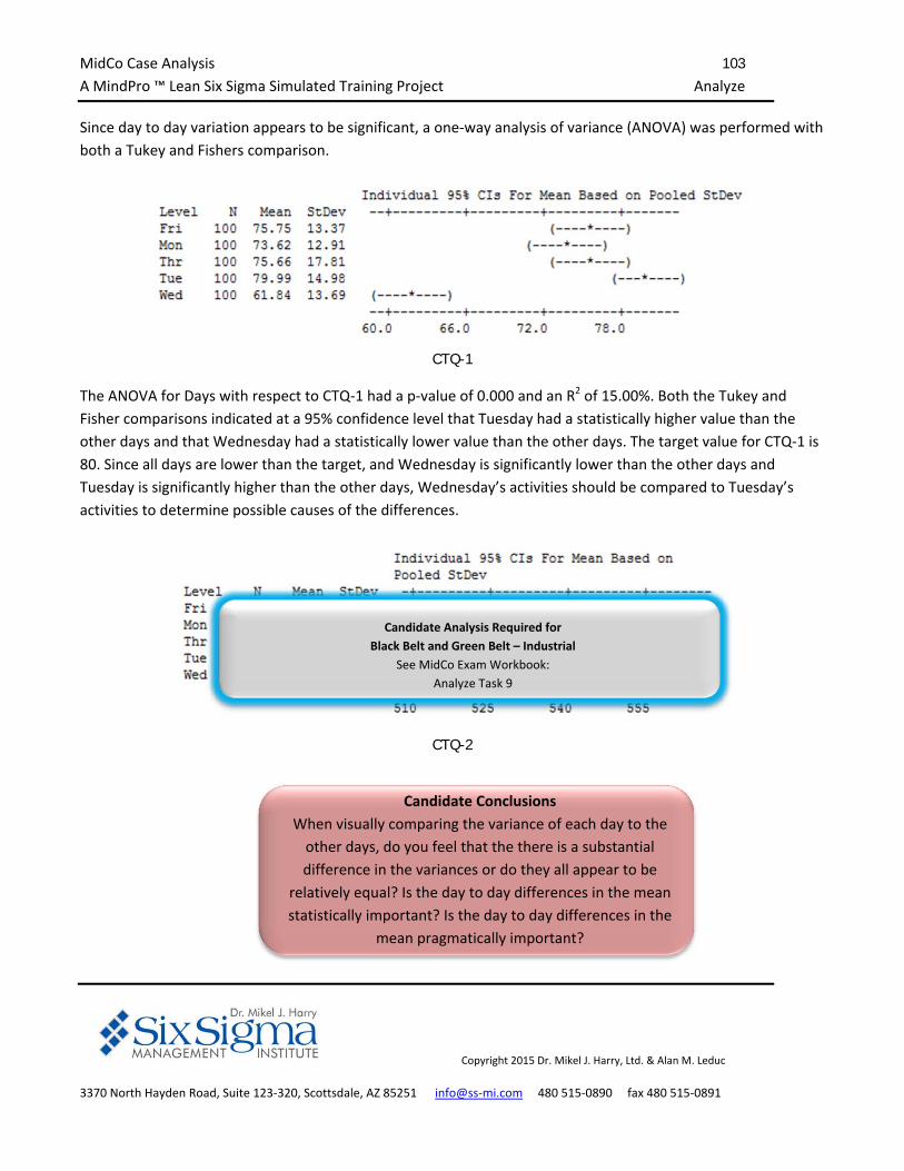
MidCo Case Analysis 103
A MindPro ™ Lean Six Sigma Simulated Training Project Analyze
Copyright 2015 Dr. Mikel J. Harry, Ltd. & Alan M. Leduc
3370 North Hayden Road, Suite 123‐320, Scottsdale, AZ 85251 info@ss‐mi.com 480 515‐0890 fax 480 515‐0891
Since day to day variation appears to be significant, a one‐way analysis of variance (ANOVA) was performed with
both a Tukey and Fishers comparison.
CTQ-1
The ANOVA for Days with respect to CTQ‐1 had a p‐value of 0.000 and an R2 of 15.00%. Both the Tukey and
Fisher comparisons indicated at a 95% confidence level that Tuesday had a statistically higher value than the
other days and that Wednesday had a statistically lower value than the other days. The target value for CTQ‐1 is
80. Since all days are lower than the target, and Wednesday is significantly lower than the other days and
Tuesday is significantly higher than the other days, Wednesday’s activities should be compared to Tuesday’s
activities to determine possible causes of the differences.
CTQ-2
Candidate Analysis Required for
Black Belt and Green Belt – Industrial
See MidCo Exam Workbook:
Analyze Task 9
Candidate Conclusions
When visually comparing the variance of each day to the
other days, do you feel that the there is a substantial
difference in the variances or do they all appear to be
relatively equal? Is the day to day differences in the mean
statistically important? Is the day to day differences in the
mean pragmatically important?
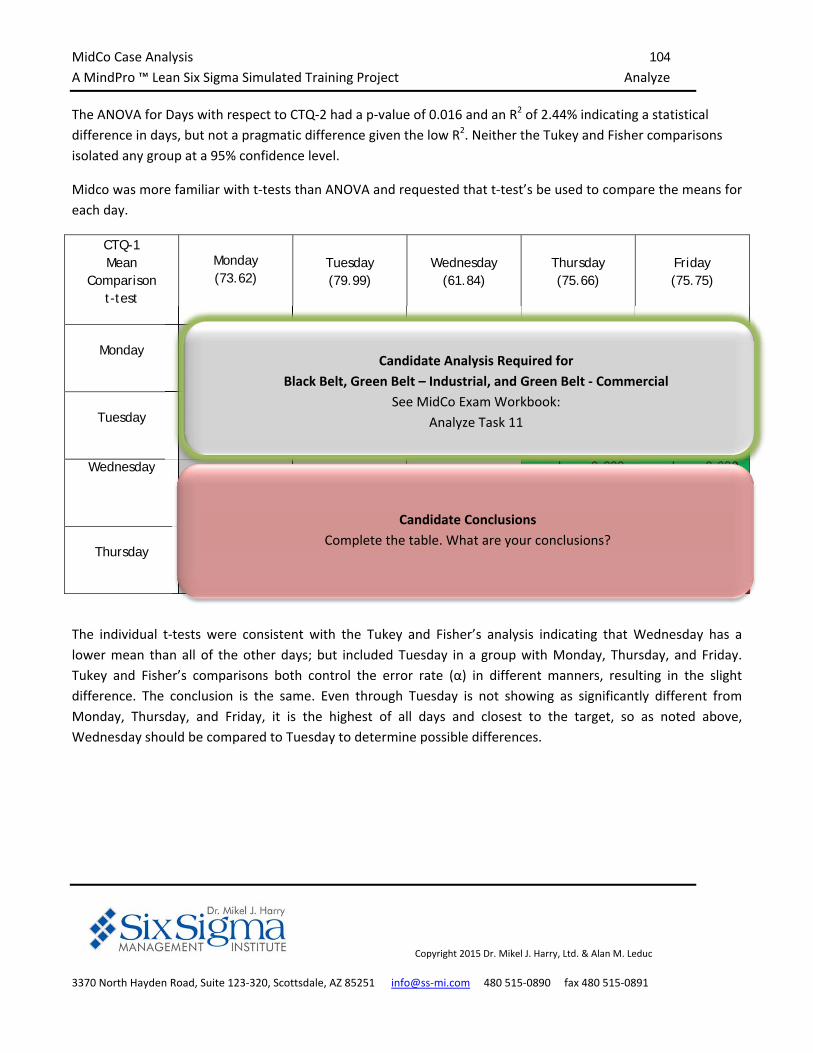
MidCo Case Analysis 104
A MindPro ™ Lean Six Sigma Simulated Training Project Analyze
Copyright 2015 Dr. Mikel J. Harry, Ltd. & Alan M. Leduc
3370 North Hayden Road, Suite 123‐320, Scottsdale, AZ 85251 info@ss‐mi.com 480 515‐0890 fax 480 515‐0891
The ANOVA for Days with respect to CTQ‐2 had a p‐value of 0.016 and an R2 of 2.44% indicating a statistical
difference in days, but not a pragmatic difference given the low R2. Neither the Tukey and Fisher comparisons
isolated any group at a 95% confidence level.
Midco was more familiar with t‐tests than ANOVA and requested that t‐test’s be used to compare the means for
each day.
CTQ-1 Mean
Comparison t-test
Monday (73.62)
Tuesday (79.99)
Wednesday (61.84)
Thursday (75.66)
Friday (75.75)
Monday p-value = 0.001
Significant Difference
p-value = 0.000 Significant Difference
p-value = 0.355 Not Significant No Difference
p-value = 0.253 Not Significant No Difference
Tuesday p-value = 0.000
Significant Difference
p-value = 0.064 Not Significant No Difference
p-value = 0.036 Significant Difference
Wednesday
p-value = 0.000 Significant Difference
p-value = 0.000 Significant Difference
Thursday p-value = 0.968 Not Significant No Difference
The individual t‐tests were consistent with the Tukey and Fisher’s analysis indicating that Wednesday has a
lower mean than all of the other days; but included Tuesday in a group with Monday, Thursday, and Friday.
Tukey and Fisher’s comparisons both control the error rate (α) in different manners, resulting in the slight
difference. The conclusion is the same. Even through Tuesday is not showing as significantly different from
Monday, Thursday, and Friday, it is the highest of all days and closest to the target, so as noted above,
Wednesday should be compared to Tuesday to determine possible differences.
Candidate Analysis Required for
Black Belt, Green Belt – Industrial, and Green Belt ‐ Commercial
See MidCo Exam Workbook:
Analyze Task 11
Candidate Conclusions
Complete the table. What are your conclusions?
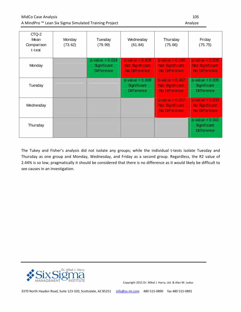
MidCo Case Analysis 105
A MindPro ™ Lean Six Sigma Simulated Training Project Analyze
Copyright 2015 Dr. Mikel J. Harry, Ltd. & Alan M. Leduc
3370 North Hayden Road, Suite 123‐320, Scottsdale, AZ 85251 info@ss‐mi.com 480 515‐0890 fax 480 515‐0891
CTQ-2 Mean
Comparison t-test
Monday (73.62)
Tuesday (79.99)
Wednesday (61.84)
Thursday (75.66)
Friday (75.75)
Monday p-value = 0.024
Significant Difference
p-value = 0.605 Not Significant No Difference
p-value = 0.140 Not Significant No Difference
p-value = 0.535 Not Significant No Difference
Tuesday p-value = 0.008
Significant Difference
p-value = 0.497 Not Significant No Difference
p-value = 0.005 Significant Difference
Wednesday p-value = 0.057 Not Significant No Difference
p-value = 0.933 No Significant No Difference
Thursday p-value = 0.041
Significant Difference
The Tukey and Fisher’s analysis did not isolate any groups; while the individual t‐tests isolate Tuesday and
Thursday as one group and Monday, Wednesday, and Friday as a second group. Regardless, the R2 value of
2.44% is so low, pragmatically it should be considered that there is no difference as it would likely be difficult to
see causes in an investigation.
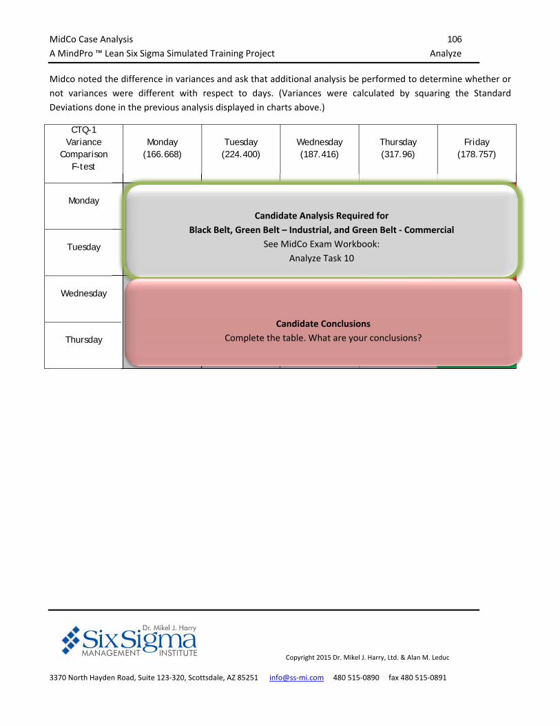
MidCo Case Analysis 106
A MindPro ™ Lean Six Sigma Simulated Training Project Analyze
Copyright 2015 Dr. Mikel J. Harry, Ltd. & Alan M. Leduc
3370 North Hayden Road, Suite 123‐320, Scottsdale, AZ 85251 info@ss‐mi.com 480 515‐0890 fax 480 515‐0891
Midco noted the difference in variances and ask that additional analysis be performed to determine whether or
not variances were different with respect to days. (Variances were calculated by squaring the Standard
Deviations done in the previous analysis displayed in charts above.)
CTQ-1 Variance
Comparison F-test
Monday (166.668)
Tuesday (224.400)
Wednesday (187.416)
Thursday (317.96)
Friday (178.757)
Monday p-value = 0.141
Not Significant No Difference
p-value = 0.561 Not Significant No Difference
p-value = 0.002 Significant Difference
p-value = 0.728 Not Significant No Difference
Tuesday p-value = 0.372 Not Significant No Difference
p-value = 0.087 Not Significant No Difference
p-value = 0.260 Not Significant No Difference
Wednesday
p-value = 0.009
Significant Difference
p-value = 0.814 Not Significant No Difference
Thursday p-value = 0.005
Significant Difference
Candidate Analysis Required for
Black Belt, Green Belt – Industrial, and Green Belt ‐ Commercial
See MidCo Exam Workbook:
Analyze Task 10
Candidate Conclusions
Complete the table. What are your conclusions?
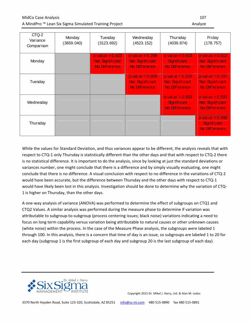
MidCo Case Analysis 107
A MindPro ™ Lean Six Sigma Simulated Training Project Analyze
Copyright 2015 Dr. Mikel J. Harry, Ltd. & Alan M. Leduc
3370 North Hayden Road, Suite 123‐320, Scottsdale, AZ 85251 info@ss‐mi.com 480 515‐0890 fax 480 515‐0891
CTQ-2 Variance
Comparison
Monday (3659.040)
Tuesday (3123.692)
Wednesday (4523.152)
Thursday (4039.874)
Friday (178.757)
Monday p-value = 0.433 Not Significant No Difference
p-value = 0.298 Not Significant No Difference
p-value = 0.623 Significant
No Difference
p-value = 0.612 Not Significant No Difference
Tuesday p-value = 0.069 Not Significant No Difference
p-value = 0.202 Not Significant No Difference
p-value = 0.197 Not Significant No Difference
Wednesday p-value = 0.583
Significant No Difference
p-value = 0.593 Not Significant No Difference
Thursday p-value = 0.988
Significant No Difference
While the values for Standard Deviation, and thus variances appear to be different, the analysis reveals that with
respect to CTQ‐1 only Thursday is statistically different than the other days and that with respect to CTQ‐2 there
is no statistical difference. It is important to do the analysis, since by looking at just the standard deviations or
variances number, one might conclude that there is a difference and by simply visually evaluating, one might
conclude that there is no difference. A visual conclusion with respect to no difference in the variations of CTQ‐2
would have been accurate, but the difference between Thursday and the other days with respect to CTQ‐1
would have likely been lost in this analysis. Investigation should be done to determine why the variation of CTQ‐
1 is higher on Thursday, than the other days.
A one‐way analysis of variance (ANOVA) was performed to determine the effect of subgroups on CTQ1 and
CTQ2 Values. A similar analysis was performed during the measure phase to determine if variation was
attributable to subgroup‐to‐subgroup (process centering issues; black noise) variations indicating a need to
focus on long term capability versus variation being attributable to natural causes or other unknown causes
(white noise) within the process. In the case of the Measure Phase analysis, the subgroups were labeled 1
through 100. In this analysis, there is a concern that time of day is an issue, so subgroups are labeled 1 to 20 for
each day (subgroup 1 is the first subgroup of each day and subgroup 20 is the last subgroup of each day).
MidCo Case Analysis 108
A MindPro ™ Lean Six Sigma Simulated Training Project Analyze
Copyright 2015 Dr. Mikel J. Harry, Ltd. & Alan M. Leduc
3370 North Hayden Road, Suite 123‐320, Scottsdale, AZ 85251 info@ss‐mi.com 480 515‐0890 fax 480 515‐0891
The figure below shows the means and confidence intervals for the twenty representative times of day. The
target value for CTQ1 Value is 80 and the upper and lower specifications are 115 and 45, respectively. While the
confidence limits for all times of the day are within specification it appears that a shift is taking place starting
with subgroup 4 and ending with subgroup 9. Subgroups 5 to 9 have a mean close to or higher than the target
while those before and after have a mean that is substantially below the target. Subgroups 5 to 9 are a better
situation than the other subgroups. Regardless of the R2 value, an investigation should be done to determine
what is being done during this time period and to determine how the results can be duplicated during the other
time periods.
Candidate Conclusions
What are the p‐values for CTQ‐1 Value and CTQ2 Value?
What is the interpretation of the p‐values? What
proportion of the variation is explained by the model? Are
CTQ‐1 Value and CTQ2 Value pragmatically significant?
Candidate Analysis Required for
Black Belt and Green Belt – Industrial
See MidCo Exam Workbook:
Analyze Task 5
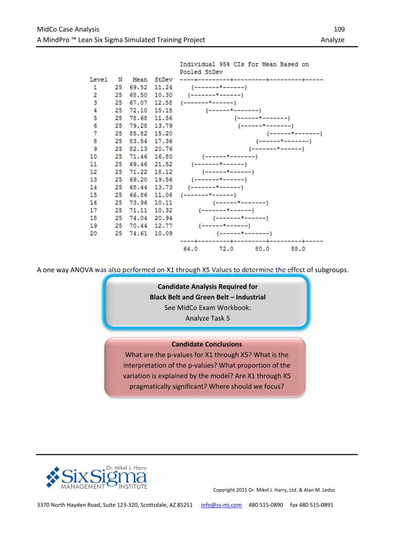
MidCo Case Analysis 109
A MindPro ™ Lean Six Sigma Simulated Training Project Analyze
Copyright 2015 Dr. Mikel J. Harry, Ltd. & Alan M. Leduc
3370 North Hayden Road, Suite 123‐320, Scottsdale, AZ 85251 info@ss‐mi.com 480 515‐0890 fax 480 515‐0891
A one way ANOVA was also performed on X1 through X5 Values to determine the effect of subgroups.
Candidate Conclusions
What are the p‐values for X1 through X5? What is the
interpretation of the p‐values? What proportion of the
variation is explained by the model? Are X1 through X5
pragmatically significant? Where should we focus?
Candidate Analysis Required for
Black Belt and Green Belt – Industrial
See MidCo Exam Workbook:
Analyze Task 5
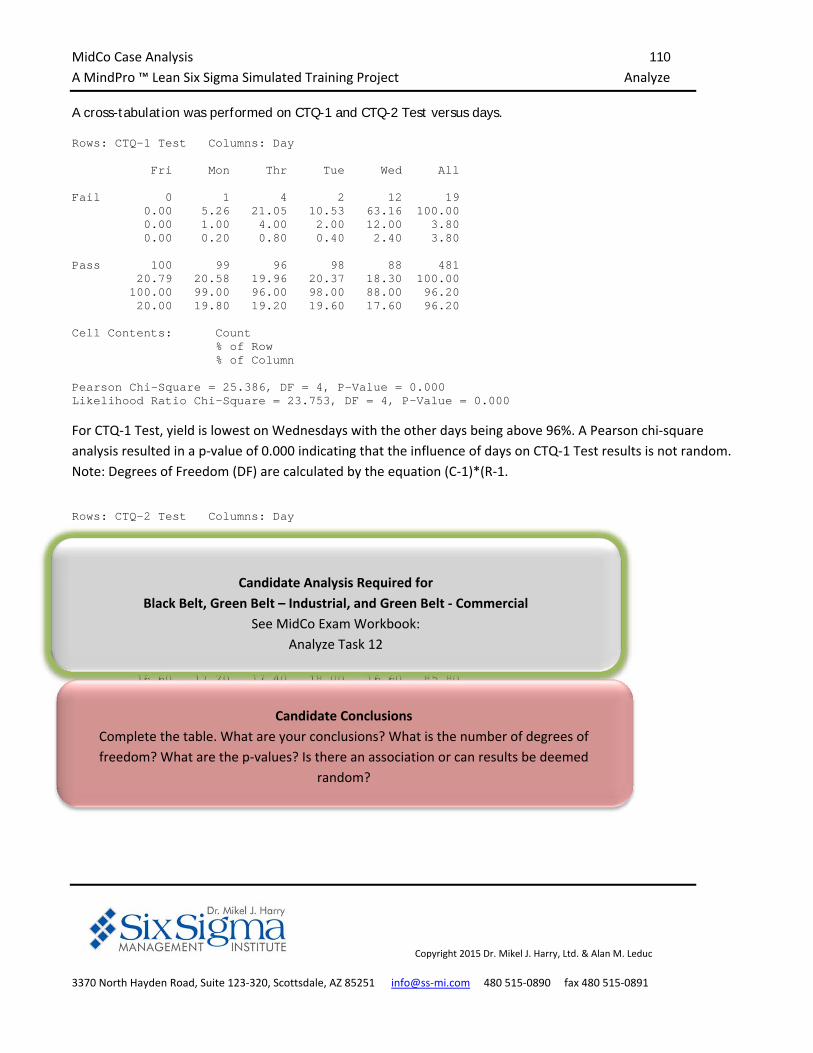
MidCo Case Analysis 110
A MindPro ™ Lean Six Sigma Simulated Training Project Analyze
Copyright 2015 Dr. Mikel J. Harry, Ltd. & Alan M. Leduc
3370 North Hayden Road, Suite 123‐320, Scottsdale, AZ 85251 info@ss‐mi.com 480 515‐0890 fax 480 515‐0891
A cross-tabulation was performed on CTQ-1 and CTQ-2 Test versus days.
Rows: CTQ-1 Test Columns: Day Fri Mon Thr Tue Wed All Fail 0 1 4 2 12 19 0.00 5.26 21.05 10.53 63.16 100.00 0.00 1.00 4.00 2.00 12.00 3.80 0.00 0.20 0.80 0.40 2.40 3.80 Pass 100 99 96 98 88 481 20.79 20.58 19.96 20.37 18.30 100.00 100.00 99.00 96.00 98.00 88.00 96.20 20.00 19.80 19.20 19.60 17.60 96.20 Cell Contents: Count % of Row % of Column Pearson Chi-Square = 25.386, DF = 4, P-Value = 0.000 Likelihood Ratio Chi-Square = 23.753, DF = 4, P-Value = 0.000
For CTQ‐1 Test, yield is lowest on Wednesdays with the other days being above 96%. A Pearson chi‐square
analysis resulted in a p‐value of 0.000 indicating that the influence of days on CTQ‐1 Test results is not random.
Note: Degrees of Freedom (DF) are calculated by the equation (C‐1)*(R‐1.
Rows: CTQ-2 Test Columns: Day Fri Mon Thr Tue Wed All Fail 17 14 13 10 17 71 23.94 19.72 18.31 14.08 23.94 100.00 17.00 14.00 13.00 10.00 17.00 14.20 3.40 2.80 2.60 2.00 3.40 14.20 Pass 83 86 87 90 83 429 19.35 20.05 20.28 20.98 19.35 100.00 83.00 86.00 87.00 90.00 83.00 85.80 16.60 17.20 17.40 18.00 16.60 85.80 Cell Contents: Count % of Row % of Column % of Total Pearson Chi-Square = 2.856, DF = 4, P-Value = 0.582 Likelihood Ratio Chi-Square = 2.936, DF = 4, P-Value = 0.569
Candidate Analysis Required for
Black Belt, Green Belt – Industrial, and Green Belt ‐ Commercial
See MidCo Exam Workbook:
Analyze Task 12
Candidate Conclusions
Complete the table. What are your conclusions? What is the number of degrees of
freedom? What are the p‐values? Is there an association or can results be deemed
random?
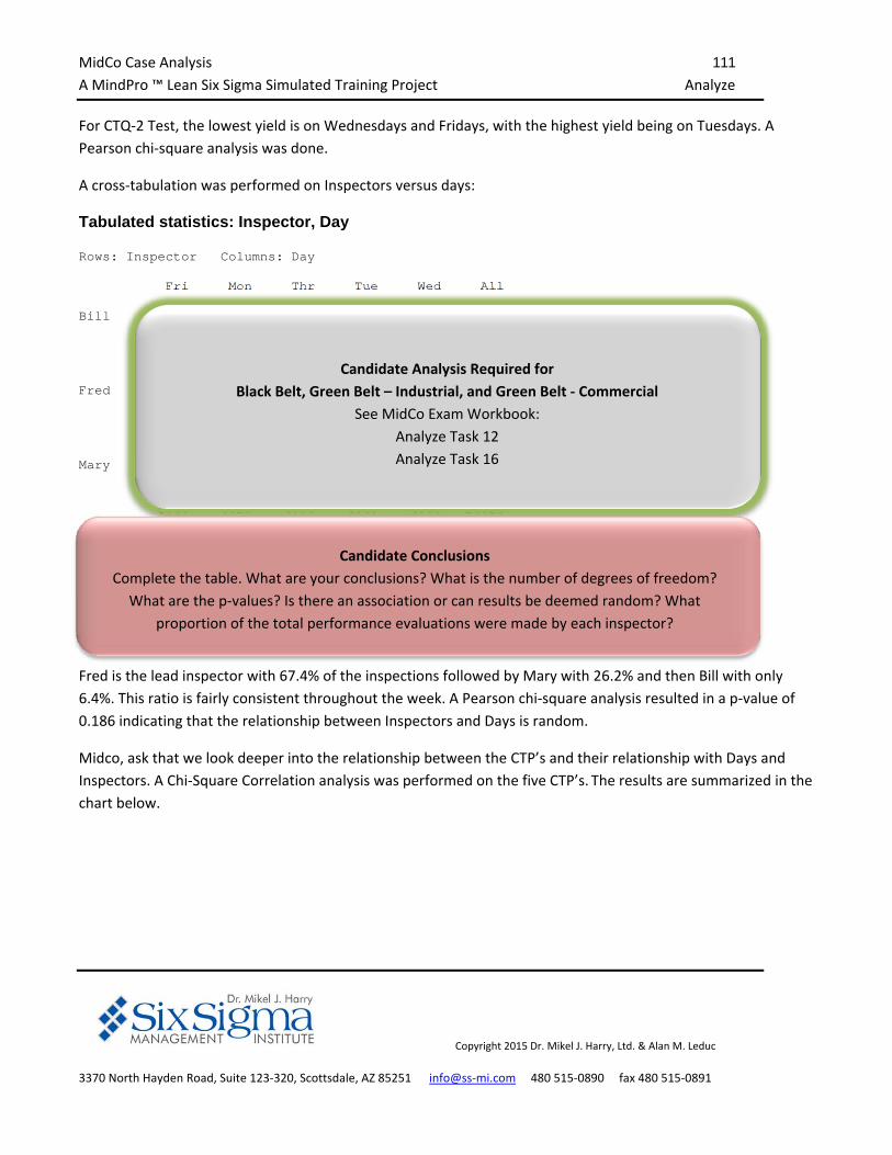
MidCo Case Analysis 111
A MindPro ™ Lean Six Sigma Simulated Training Project Analyze
Copyright 2015 Dr. Mikel J. Harry, Ltd. & Alan M. Leduc
3370 North Hayden Road, Suite 123‐320, Scottsdale, AZ 85251 info@ss‐mi.com 480 515‐0890 fax 480 515‐0891
For CTQ‐2 Test, the lowest yield is on Wednesdays and Fridays, with the highest yield being on Tuesdays. A
Pearson chi‐square analysis was done.
A cross‐tabulation was performed on Inspectors versus days:
Tabulated statistics: Inspector, Day Rows: Inspector Columns: Day Fri Mon Thr Tue Wed All Bill 7 10 5 4 6 32 21.88 31.25 15.63 12.50 18.75 100.00 7.00 10.00 5.00 4.00 6.00 6.40 1.40 2.00 1.00 0.80 1.20 6.40 Fred 60 59 75 73 70 337 17.80 17.51 22.26 21.66 20.77 100.00 60.00 59.00 75.00 73.00 70.00 67.40 12.00 11.80 15.00 14.60 14.00 67.40 Mary 33 31 20 23 24 131 25.19 23.66 15.27 17.56 18.32 100.00 33.00 31.00 20.00 23.00 24.00 26.20 6.60 6.20 4.00 4.60 4.80 26.20 Cell Contents: Count % of Row % of Column Pearson Chi-Square = 11.281, DF = 8, P-Value = 0.186 Likelihood Ratio Chi-Square = 11.149, DF = 8, P-Value = 0.193
Fred is the lead inspector with 67.4% of the inspections followed by Mary with 26.2% and then Bill with only
6.4%. This ratio is fairly consistent throughout the week. A Pearson chi‐square analysis resulted in a p‐value of
0.186 indicating that the relationship between Inspectors and Days is random.
Midco, ask that we look deeper into the relationship between the CTP’s and their relationship with Days and
Inspectors. A Chi‐Square Correlation analysis was performed on the five CTP’s. The results are summarized in the
chart below.
Candidate Analysis Required for
Black Belt, Green Belt – Industrial, and Green Belt ‐ Commercial
See MidCo Exam Workbook:
Analyze Task 12
Analyze Task 16
Candidate Conclusions
Complete the table. What are your conclusions? What is the number of degrees of freedom?
What are the p‐values? Is there an association or can results be deemed random? What
proportion of the total performance evaluations were made by each inspector?
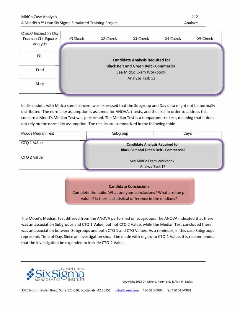
MidCo Case Analysis 112
A MindPro ™ Lean Six Sigma Simulated Training Project Analyze
Copyright 2015 Dr. Mikel J. Harry, Ltd. & Alan M. Leduc
3370 North Hayden Road, Suite 123‐320, Scottsdale, AZ 85251 info@ss‐mi.com 480 515‐0890 fax 480 515‐0891
Check/Inspector/Day Pearson Chi-Square
Analysis
X1Check X2 Check X3 Check X4 Check X5 Check
Bill Invalid
Invalid Invalid P = 0.656 Random
P = 0.078 Random
Fred P = 0.344 Random
P = 0.032 Association
P = 0.991 Random
P = 0.001 Association
P = 0.000 Association
Mary p = 0.323 Random
Invalid P = 0.722 Random
Invalid P = 0.000
Association
In discussions with Midco some concern was expressed that the Subgroup and Day data might not be normally
distributed. The normality assumption is assumed for ANOVA, t‐tests, and the like. In order to address this
concern a Mood’s Median Test was performed. The Median Test is a nonparametric test, meaning that it does
not rely on the normality assumption. The results are summarized in the following table.
Moods Median Test Subgroup Days
CTQ 1 Value p = 0.000 Difference
p = 0.000 Difference
CTQ 2 Value p = 0.007 Difference
p = 0.267 No Difference
The Mood’s Median Test differed from the ANOVA performed on subgroups. The ANOVA indicated that there
was an association Subgroups and CTQ 1 Value, but not CTQ 2 Value, while the Median Test concluded there
was an association between Subgroups and both CTQ 1 and CTQ Values. As a reminder, in this case Subgroups
represents Time of Day. Since an investigation should be made with regard to CTQ‐1 Value, it is recommended
that the investigation be expanded to include CTQ‐2 Value.
Candidate Analysis Required for
Black Belt and Green Belt ‐ Commercial
See MidCo Exam Workbook:
Analyze Task 13
Candidate Conclusions
Complete the table. What are your conclusions? What are the p‐
values? Is there a statistical difference in the medians?
Candidate Analysis Required for
Black Belt and Green Belt ‐ Commercial
See MidCo Exam Workbook:
Analyze Task 14
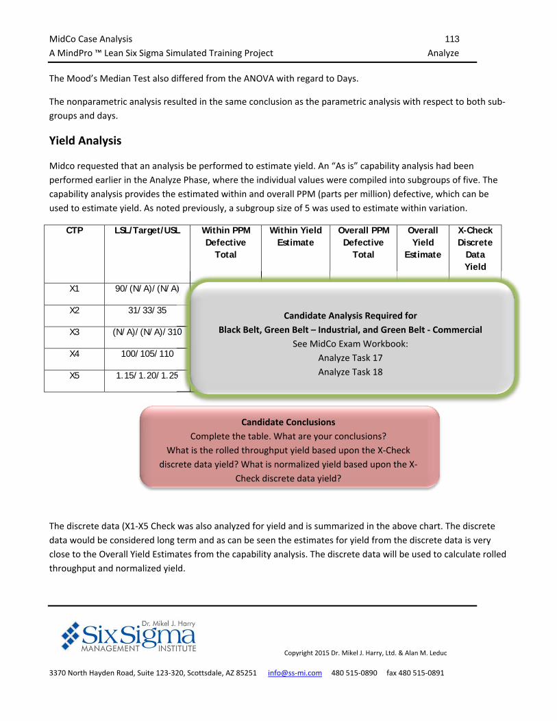
MidCo Case Analysis 113
A MindPro ™ Lean Six Sigma Simulated Training Project Analyze
Copyright 2015 Dr. Mikel J. Harry, Ltd. & Alan M. Leduc
3370 North Hayden Road, Suite 123‐320, Scottsdale, AZ 85251 info@ss‐mi.com 480 515‐0890 fax 480 515‐0891
The Mood’s Median Test also differed from the ANOVA with regard to Days.
The nonparametric analysis resulted in the same conclusion as the parametric analysis with respect to both sub‐
groups and days.
Yield Analysis
Midco requested that an analysis be performed to estimate yield. An “As is” capability analysis had been
performed earlier in the Analyze Phase, where the individual values were compiled into subgroups of five. The
capability analysis provides the estimated within and overall PPM (parts per million) defective, which can be
used to estimate yield. As noted previously, a subgroup size of 5 was used to estimate within variation.
CTP LSL/Target/USL Within PPM Defective
Total
Within Yield Estimate
Overall PPM Defective
Total
Overall Yield
Estimate
X-Check Discrete
Data Yield
X1 90/(N/A)/(N/A) 149,353.31 85.06% 149,664.78 85.03% 86.00%
X2 31/33/35 39,028.80 96.10% 161,192.08 83.88% 83.80%
X3 (N/A)/(N/A)/310 58,912.75 94.11% 79,388.80 92.06% 91.40%
X4 100/105/110 363,561.24 63.64% 457,078.73 54.29% 54.40%
X5 1.15/1.20/1.25 594,254.75 40.57% 526,305.80 47.37% 49.00%
The discrete data (X1‐X5 Check was also analyzed for yield and is summarized in the above chart. The discrete
data would be considered long term and as can be seen the estimates for yield from the discrete data is very
close to the Overall Yield Estimates from the capability analysis. The discrete data will be used to calculate rolled
throughput and normalized yield.
Candidate Conclusions
Complete the table. What are your conclusions?
What is the rolled throughput yield based upon the X‐Check
discrete data yield? What is normalized yield based upon the X‐
Check discrete data yield?
Candidate Analysis Required for
Black Belt, Green Belt – Industrial, and Green Belt ‐ Commercial
See MidCo Exam Workbook:
Analyze Task 17
Analyze Task 18

MidCo Case Analysis 114
A MindPro ™ Lean Six Sigma Simulated Training Project Analyze
Copyright 2015 Dr. Mikel J. Harry, Ltd. & Alan M. Leduc
3370 North Hayden Road, Suite 123‐320, Scottsdale, AZ 85251 info@ss‐mi.com 480 515‐0890 fax 480 515‐0891
The Normalized Yield provides the minimum Throughput Yield for each step of the process to achieve a given
Rolled Throughput Yield. While not the arithmetic average it can be considered the average yield of all of the
processes. By comparing the Discrete Yields of each variable to the Normalized Yield, it can be seen that CTP’s
X4 and X5 are below average, while CTP’s X1, X2, and X3 are above average.
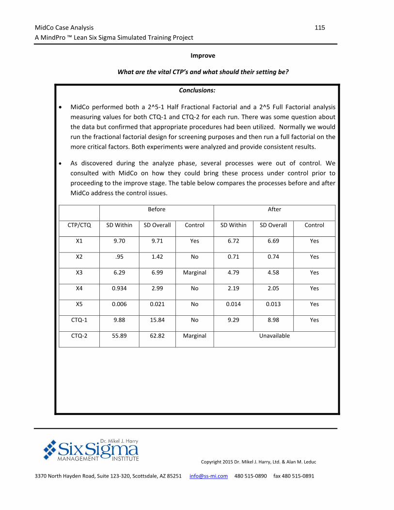
MidCo Case Analysis 115
A MindPro ™ Lean Six Sigma Simulated Training Project
Copyright 2015 Dr. Mikel J. Harry, Ltd. & Alan M. Leduc
3370 North Hayden Road, Suite 123‐320, Scottsdale, AZ 85251 info@ss‐mi.com 480 515‐0890 fax 480 515‐0891
Improve
What are the vital CTP’s and what should their setting be?
Conclusions:
MidCo performed both a 2^5‐1 Half Fractional Factorial and a 2^5 Full Factorial analysis
measuring values for both CTQ‐1 and CTQ‐2 for each run. There was some question about
the data but confirmed that appropriate procedures had been utilized. Normally we would
run the fractional factorial design for screening purposes and then run a full factorial on the
more critical factors. Both experiments were analyzed and provide consistent results.
As discovered during the analyze phase, several processes were out of control. We
consulted with MidCo on how they could bring these process under control prior to
proceeding to the improve stage. The table below compares the processes before and after
MidCo address the control issues.
Before After
CTP/CTQ SD Within SD Overall Control SD Within SD Overall Control
X1 9.70 9.71 Yes 6.72 6.69 Yes
X2 .95 1.42 No 0.71 0.74 Yes
X3 6.29 6.99 Marginal 4.79 4.58 Yes
X4 0.934 2.99 No 2.19 2.05 Yes
X5 0.006 0.021 No 0.014 0.013 Yes
CTQ‐1 9.88 15.84 No 9.29 8.98 Yes
CTQ‐2 55.89 62.82 Marginal Unavailable
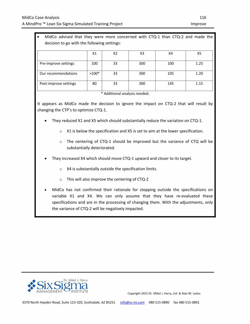
MidCo Case Analysis 116
A MindPro ™ Lean Six Sigma Simulated Training Project Improve
Copyright 2015 Dr. Mikel J. Harry, Ltd. & Alan M. Leduc
3370 North Hayden Road, Suite 123‐320, Scottsdale, AZ 85251 info@ss‐mi.com 480 515‐0890 fax 480 515‐0891
MidCo advised that they were more concerned with CTQ‐1 than CTQ‐2 and made the
decision to go with the following settings:
X1 X2 X3 X4 X5
Pre‐improve settings 100 33 300 100 1.25
Our recommendations >100* 33 300 105 1.20
Post‐improve settings 80 33 300 145 1.15
* Additional analysis needed.
It appears as MidCo made the decision to ignore the impact on CTQ‐2 that will result by
changing the CTP’s to optimize CTQ‐1.
They reduced X1 and X5 which should substantially reduce the variation on CTQ‐1.
o X1 is below the specification and X5 is set to aim at the lower specification.
o The centering of CTQ‐1 should be improved but the variance of CTQ will be
substantially deteriorated.
They increased X4 which should move CTQ‐1 upward and closer to its target.
o X4 is substantially outside the specification limits.
o This will also improve the centering of CTQ‐2
MidCo has not confirmed their rationale for stepping outside the specifications on
variable X1 and X4. We can only assume that they have re‐evaluated these
specifications and are in the processing of changing them. With the adjustments, only
the variance of CTQ‐2 will be negatively impacted.
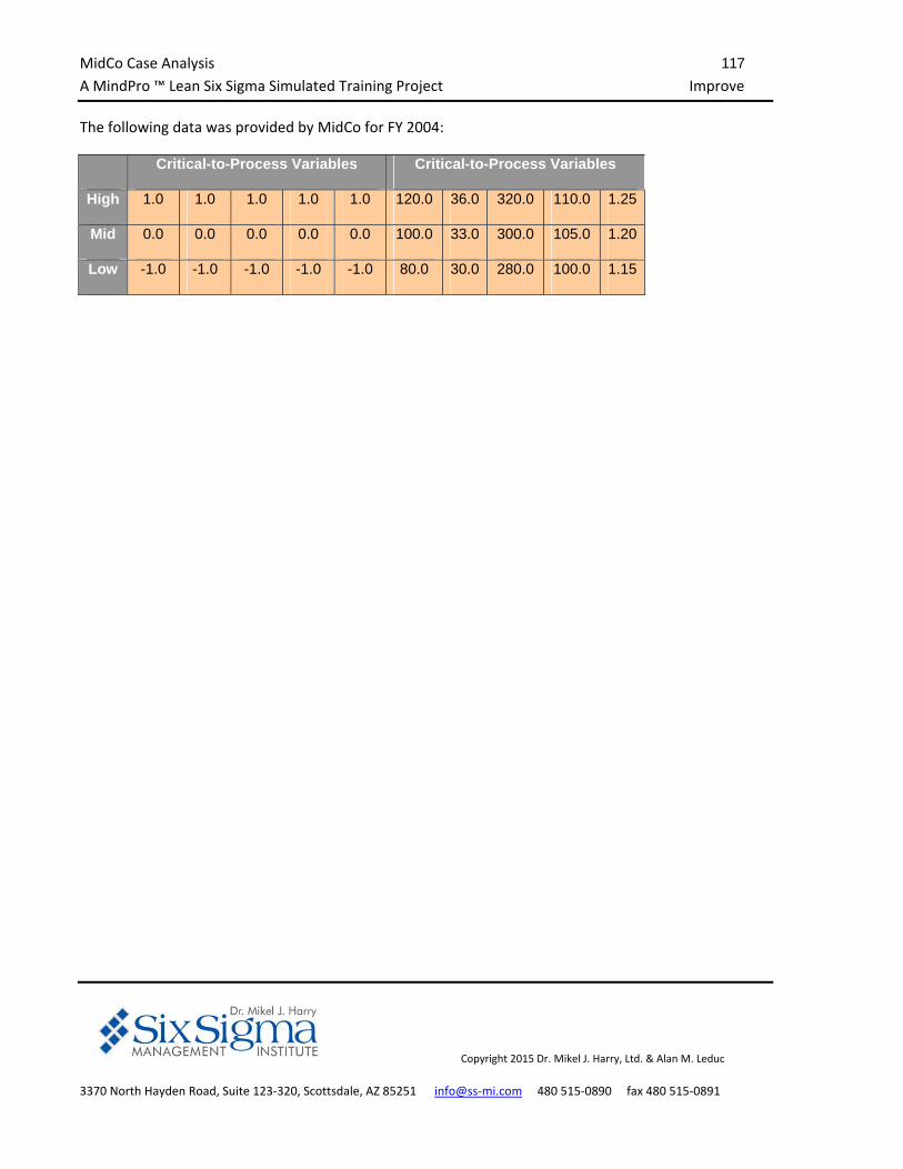
MidCo Case Analysis 117
A MindPro ™ Lean Six Sigma Simulated Training Project Improve
Copyright 2015 Dr. Mikel J. Harry, Ltd. & Alan M. Leduc
3370 North Hayden Road, Suite 123‐320, Scottsdale, AZ 85251 info@ss‐mi.com 480 515‐0890 fax 480 515‐0891
The following data was provided by MidCo for FY 2004:
Critical-to-Process Variables Critical-to-Process Variables
High 1.0 1.0 1.0 1.0 1.0 120.0 36.0 320.0 110.0 1.25
Mid 0.0 0.0 0.0 0.0 0.0 100.0 33.0 300.0 105.0 1.20
Low -1.0 -1.0 -1.0 -1.0 -1.0 80.0 30.0 280.0 100.0 1.15
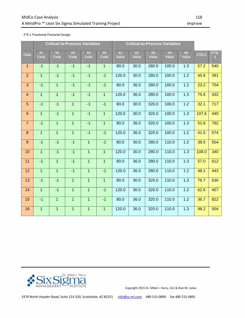
MidCo Case Analysis 118
A MindPro ™ Lean Six Sigma Simulated Training Project Improve
Copyright 2015 Dr. Mikel J. Harry, Ltd. & Alan M. Leduc
3370 North Hayden Road, Suite 123‐320, Scottsdale, AZ 85251 info@ss‐mi.com 480 515‐0890 fax 480 515‐0891
2^5-1 Fractional Factorial Design
Critical-to-Process Variables Critical-to-Process Variables
Case X1
Code X2
Code X3
Code X4
Code X5
Code X1
Value X2
Value X3
Value X4
Value X5
Value CTQ-1
CTQ-2
1 -1 -1 -1 -1 1 80.0 30.0 280.0 100.0 1.3 57.2 540
2 1 -1 -1 -1 -1 120.0 30.0 280.0 100.0 1.2 45.6 391
3 -1 1 -1 -1 -1 80.0 36.0 280.0 100.0 1.2 23.2 704
4 1 1 -1 -1 1 120.0 36.0 280.0 100.0 1.3 75.6 432
5 -1 -1 1 -1 -1 80.0 30.0 320.0 100.0 1.2 32.1 717
6 1 -1 1 -1 1 120.0 30.0 320.0 100.0 1.3 107.6 440
7 -1 1 1 -1 1 80.0 36.0 320.0 100.0 1.3 51.6 792
8 1 1 1 -1 -1 120.0 36.0 320.0 100.0 1.2 41.5 574
9 -1 -1 -1 1 -1 80.0 30.0 280.0 110.0 1.2 39.5 554
10 1 -1 -1 1 1 120.0 30.0 280.0 110.0 1.3 108.0 340
11 -1 1 -1 1 1 80.0 36.0 280.0 110.0 1.3 57.0 612
12 1 1 -1 1 -1 120.0 36.0 280.0 110.0 1.2 48.1 443
13 -1 -1 1 1 1 80.0 30.0 320.0 110.0 1.3 76.7 630
14 1 -1 1 1 -1 120.0 30.0 320.0 110.0 1.2 62.6 457
15 -1 1 1 1 -1 80.0 36.0 320.0 110.0 1.2 36.7 822
16 1 1 1 1 1 120.0 36.0 320.0 110.0 1.3 98.2 504
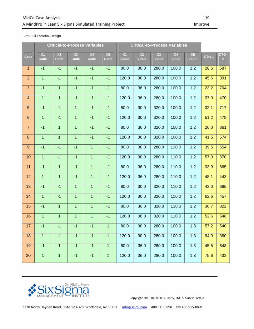
MidCo Case Analysis 119
A MindPro ™ Lean Six Sigma Simulated Training Project Improve
Copyright 2015 Dr. Mikel J. Harry, Ltd. & Alan M. Leduc
3370 North Hayden Road, Suite 123‐320, Scottsdale, AZ 85251 info@ss‐mi.com 480 515‐0890 fax 480 515‐0891
2^5 Full Factorial Design
Critical-to-Process Variables Critical-to-Process Variables
Case X1
Code X2
Code X3
Code X4
Code X5
Code X1
Value X2
Value X3
Value X4
Value X5
Value CTQ-1
CTQ-2
1 -1 -1 -1 -1 -1 80.0 30.0 280.0 100.0 1.2 28.6 587
2 1 -1 -1 -1 -1 120.0 30.0 280.0 100.0 1.2 45.6 391
3 -1 1 -1 -1 -1 80.0 36.0 280.0 100.0 1.2 23.2 704
4 1 1 -1 -1 -1 120.0 36.0 280.0 100.0 1.2 37.0 470
5 -1 -1 1 -1 -1 80.0 30.0 320.0 100.0 1.2 32.1 717
6 1 -1 1 -1 -1 120.0 30.0 320.0 100.0 1.2 51.2 478
7 -1 1 1 -1 -1 80.0 36.0 320.0 100.0 1.2 26.0 861
8 1 1 1 -1 -1 120.0 36.0 320.0 100.0 1.2 41.5 574
9 -1 -1 -1 1 -1 80.0 30.0 280.0 110.0 1.2 39.5 554
10 1 -1 -1 1 -1 120.0 30.0 280.0 110.0 1.2 57.0 370
11 -1 1 -1 1 -1 80.0 36.0 280.0 110.0 1.2 33.9 665
12 1 1 -1 1 -1 120.0 36.0 280.0 110.0 1.2 48.1 443
13 -1 -1 1 1 -1 80.0 30.0 320.0 110.0 1.2 43.0 685
14 1 -1 1 1 -1 120.0 30.0 320.0 110.0 1.2 62.6 457
15 -1 1 1 1 -1 80.0 36.0 320.0 110.0 1.2 36.7 822
16 1 1 1 1 -1 120.0 36.0 320.0 110.0 1.2 52.6 548
17 -1 -1 -1 -1 1 80.0 30.0 280.0 100.0 1.3 57.2 540
18 1 -1 -1 -1 1 120.0 30.0 280.0 100.0 1.3 94.9 360
19 -1 1 -1 -1 1 80.0 36.0 280.0 100.0 1.3 45.5 648
20 1 1 -1 -1 1 120.0 36.0 280.0 100.0 1.3 75.6 432
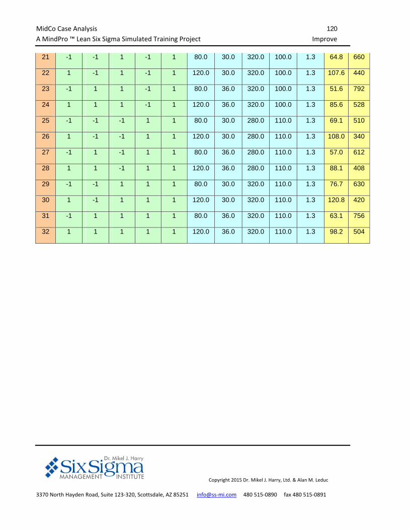
MidCo Case Analysis 120
A MindPro ™ Lean Six Sigma Simulated Training Project Improve
Copyright 2015 Dr. Mikel J. Harry, Ltd. & Alan M. Leduc
3370 North Hayden Road, Suite 123‐320, Scottsdale, AZ 85251 info@ss‐mi.com 480 515‐0890 fax 480 515‐0891
21 -1 -1 1 -1 1 80.0 30.0 320.0 100.0 1.3 64.8 660
22 1 -1 1 -1 1 120.0 30.0 320.0 100.0 1.3 107.6 440
23 -1 1 1 -1 1 80.0 36.0 320.0 100.0 1.3 51.6 792
24 1 1 1 -1 1 120.0 36.0 320.0 100.0 1.3 85.6 528
25 -1 -1 -1 1 1 80.0 30.0 280.0 110.0 1.3 69.1 510
26 1 -1 -1 1 1 120.0 30.0 280.0 110.0 1.3 108.0 340
27 -1 1 -1 1 1 80.0 36.0 280.0 110.0 1.3 57.0 612
28 1 1 -1 1 1 120.0 36.0 280.0 110.0 1.3 88.1 408
29 -1 -1 1 1 1 80.0 30.0 320.0 110.0 1.3 76.7 630
30 1 -1 1 1 1 120.0 30.0 320.0 110.0 1.3 120.8 420
31 -1 1 1 1 1 80.0 36.0 320.0 110.0 1.3 63.1 756
32 1 1 1 1 1 120.0 36.0 320.0 110.0 1.3 98.2 504
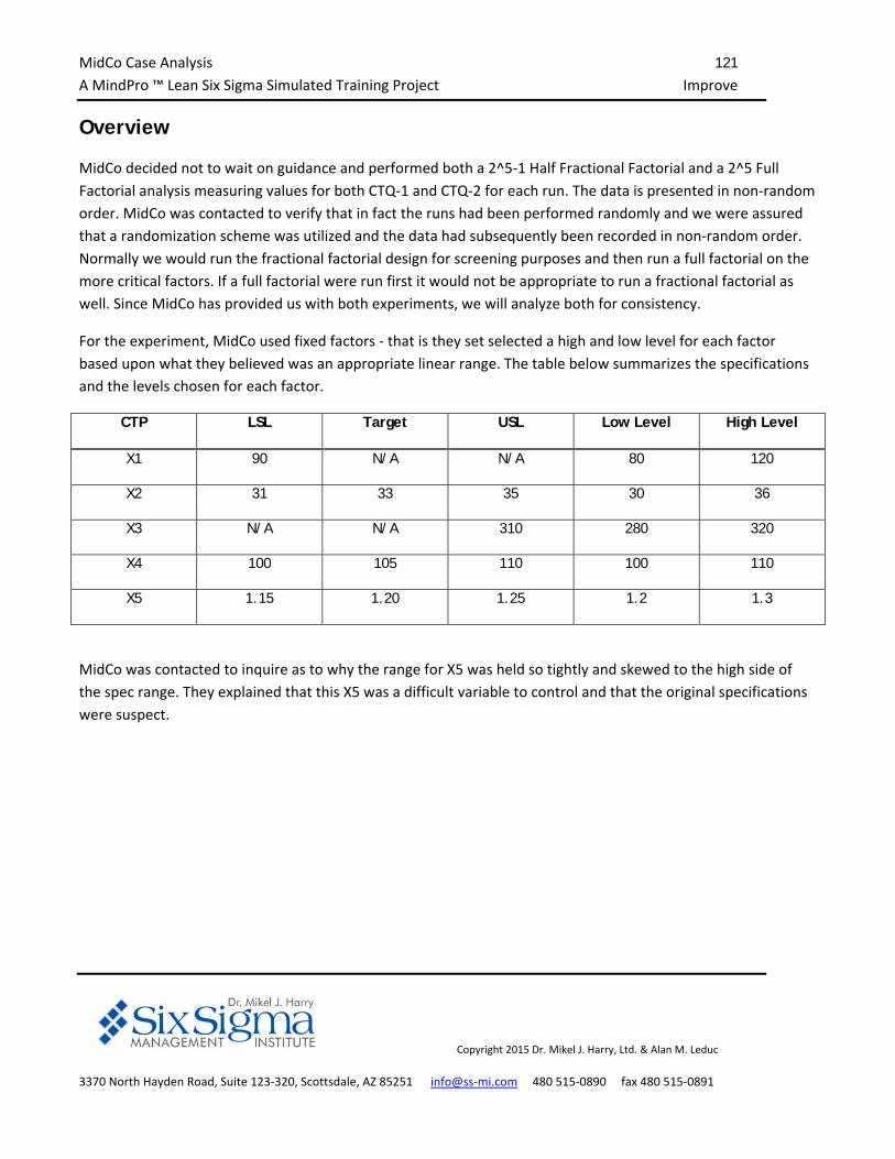
MidCo Case Analysis 121
A MindPro ™ Lean Six Sigma Simulated Training Project Improve
Copyright 2015 Dr. Mikel J. Harry, Ltd. & Alan M. Leduc
3370 North Hayden Road, Suite 123‐320, Scottsdale, AZ 85251 info@ss‐mi.com 480 515‐0890 fax 480 515‐0891
Overview
MidCo decided not to wait on guidance and performed both a 2^5‐1 Half Fractional Factorial and a 2^5 Full
Factorial analysis measuring values for both CTQ‐1 and CTQ‐2 for each run. The data is presented in non‐random
order. MidCo was contacted to verify that in fact the runs had been performed randomly and we were assured
that a randomization scheme was utilized and the data had subsequently been recorded in non‐random order.
Normally we would run the fractional factorial design for screening purposes and then run a full factorial on the
more critical factors. If a full factorial were run first it would not be appropriate to run a fractional factorial as
well. Since MidCo has provided us with both experiments, we will analyze both for consistency.
For the experiment, MidCo used fixed factors ‐ that is they set selected a high and low level for each factor
based upon what they believed was an appropriate linear range. The table below summarizes the specifications
and the levels chosen for each factor.
CTP LSL Target USL Low Level High Level
X1 90 N/A N/A 80 120
X2 31 33 35 30 36
X3 N/A N/A 310 280 320
X4 100 105 110 100 110
X5 1.15 1.20 1.25 1.2 1.3
MidCo was contacted to inquire as to why the range for X5 was held so tightly and skewed to the high side of
the spec range. They explained that this X5 was a difficult variable to control and that the original specifications
were suspect.
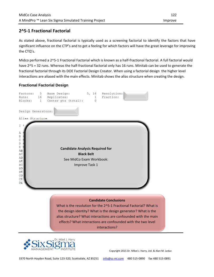
MidCo Case Analysis 122
A MindPro ™ Lean Six Sigma Simulated Training Project Improve
Copyright 2015 Dr. Mikel J. Harry, Ltd. & Alan M. Leduc
3370 North Hayden Road, Suite 123‐320, Scottsdale, AZ 85251 info@ss‐mi.com 480 515‐0890 fax 480 515‐0891
2^5‐1 Fractional Factorial
As stated above, fractional factorial is typically used as a screening factorial to identify the factors that have
significant influence on the CTP’s and to get a feeling for which factors will have the great leverage for improving
the CTQ’s.
Midco performed a 2^5‐1 Fractional Factorial which is known as a half‐fractional factorial. A full factorial would
have 2^5 = 32 runs. Whereas the half‐fractional factorial only has 16 runs. Minitab can be used to generate the
fractional factorial through its DOE Factorial Design Creator. When using a factorial design the higher level
interactions are aliased with the main effects. Minitab shows the alias structure when creating the design.
Fractional Factorial Design Factors: 5 Base Design: 5, 16 Resolution: V Runs: 16 Replicates: 1 Fraction: 1/2 Blocks: 1 Center pts (total): 0 Design Generators: E = ABCD Alias Structure I + ABCDE A + BCDE B + ACDE C + ABDE D + ABCE E + ABCD AB + CDE AC + BDE AD + BCE AE + BCD BC + ADE BD + ACE BE + ACD CD + ABE CE + ABD DE + ABC
CTQ‐1
Candidate Conclusions
What is the resolution for the 2^5‐1 Fractional Factorial? What is
the design identity? What is the design generator? What is the
alias structure? What interactions are confounded with the main
effects? What interactions are confounded with the two level
interactions?
Candidate Analysis Required for
Black Belt
See MidCo Exam Workbook:
Improve Task 1
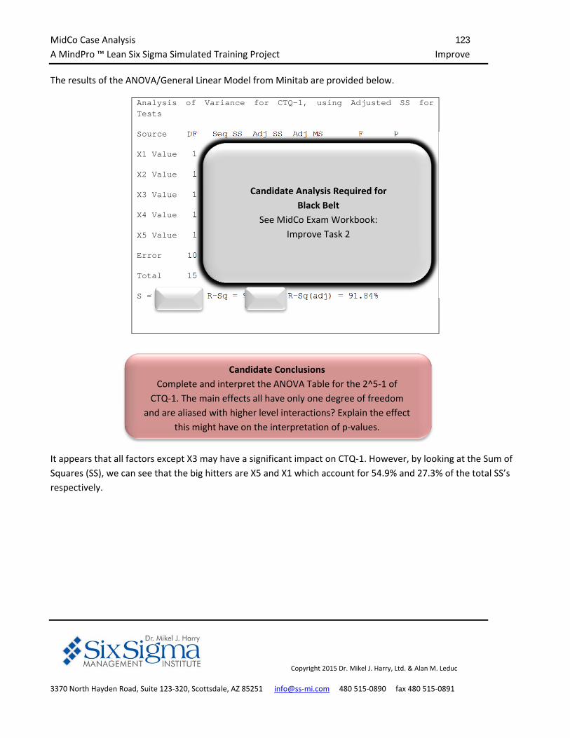
MidCo Case Analysis 123
A MindPro ™ Lean Six Sigma Simulated Training Project Improve
Copyright 2015 Dr. Mikel J. Harry, Ltd. & Alan M. Leduc
3370 North Hayden Road, Suite 123‐320, Scottsdale, AZ 85251 info@ss‐mi.com 480 515‐0890 fax 480 515‐0891
The results of the ANOVA/General Linear Model from Minitab are provided below.
Analysis of Variance for CTQ-1, using Adjusted SS for Tests
Source DF Seq SS Adj SS Adj MS F P
X1 Value 1 2840.9 2840.9 2840.9 50.04 0.000
X2 Value 1 592.9 592.9 592.9 10.44 0.009
X3 Value 1 174.2 174.2 174.2 3.07 0.110
X4 Value 1 533.6 533.6 533.6 9.40 0.012
X5 Value 1 5722.9 5722.9 5722.9 100.80 0.000
Error 10 567.7 567.7 56.8
Total 15 10432.3
S = 7.53489 R-Sq = 94.56% R-Sq(adj) = 91.84%
It appears that all factors except X3 may have a significant impact on CTQ‐1. However, by looking at the Sum of
Squares (SS), we can see that the big hitters are X5 and X1 which account for 54.9% and 27.3% of the total SS’s
respectively.
Candidate Analysis Required for
Black Belt
See MidCo Exam Workbook:
Improve Task 2
Candidate Conclusions
Complete and interpret the ANOVA Table for the 2^5‐1 of
CTQ‐1. The main effects all have only one degree of freedom
and are aliased with higher level interactions? Explain the effect
this might have on the interpretation of p‐values.
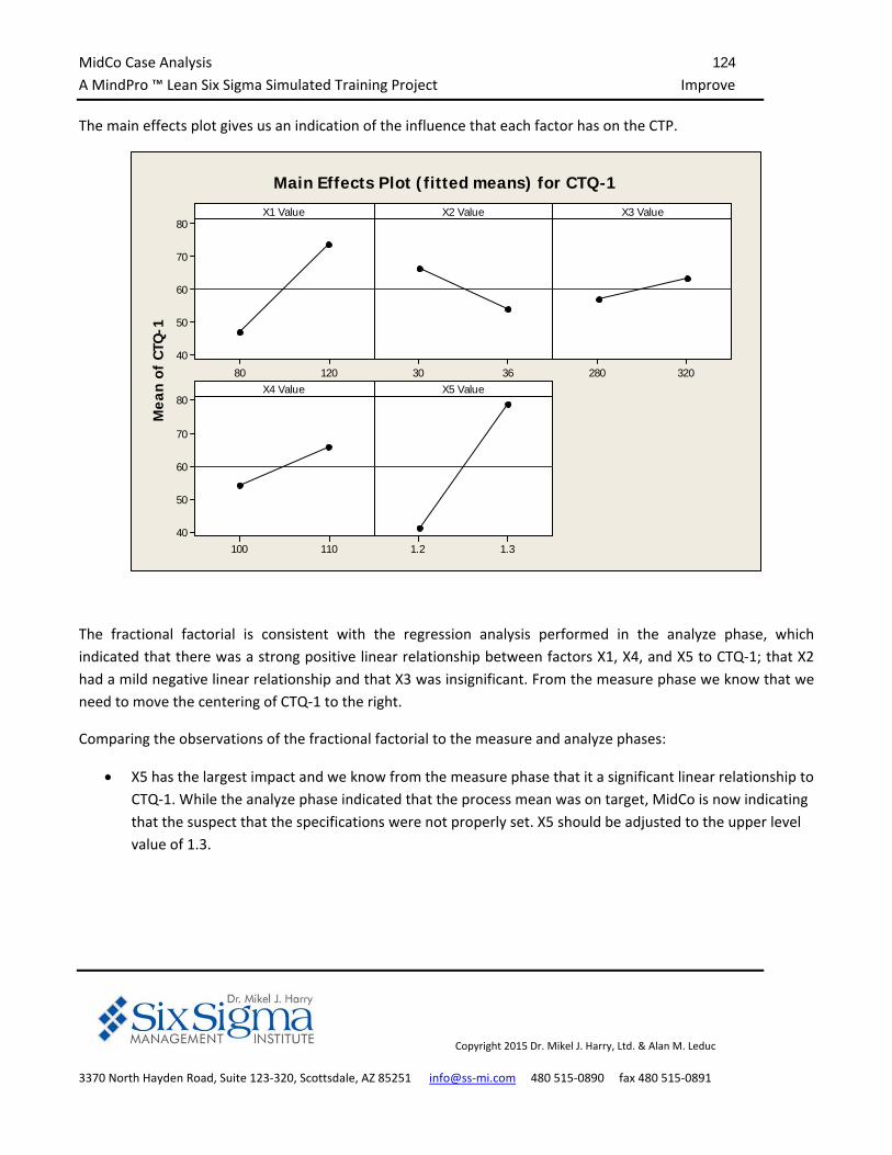
MidCo Case Analysis 124
A MindPro ™ Lean Six Sigma Simulated Training Project Improve
Copyright 2015 Dr. Mikel J. Harry, Ltd. & Alan M. Leduc
3370 North Hayden Road, Suite 123‐320, Scottsdale, AZ 85251 info@ss‐mi.com 480 515‐0890 fax 480 515‐0891
The main effects plot gives us an indication of the influence that each factor has on the CTP.
Mea
n of
CTQ
-1
12080
80
70
60
50
40
3630 320280
110100
80
70
60
50
401.31.2
X1 Value X2 Value X3 Value
X4 Value X5 Value
Main Effects Plot (fitted means) for CTQ-1
The fractional factorial is consistent with the regression analysis performed in the analyze phase, which
indicated that there was a strong positive linear relationship between factors X1, X4, and X5 to CTQ‐1; that X2
had a mild negative linear relationship and that X3 was insignificant. From the measure phase we know that we
need to move the centering of CTQ‐1 to the right.
Comparing the observations of the fractional factorial to the measure and analyze phases:
X5 has the largest impact and we know from the measure phase that it a significant linear relationship to
CTQ‐1. While the analyze phase indicated that the process mean was on target, MidCo is now indicating
that the suspect that the specifications were not properly set. X5 should be adjusted to the upper level
value of 1.3.
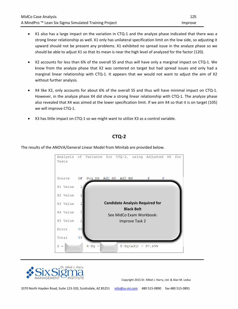
MidCo Case Analysis 125
A MindPro ™ Lean Six Sigma Simulated Training Project Improve
Copyright 2015 Dr. Mikel J. Harry, Ltd. & Alan M. Leduc
3370 North Hayden Road, Suite 123‐320, Scottsdale, AZ 85251 info@ss‐mi.com 480 515‐0890 fax 480 515‐0891
X1 also has a large impact on the variation in CTQ‐1 and the analyze phase indicated that there was a
strong linear relationship as well. X1 only has unilateral specification limit on the low side, so adjusting it
upward should not be present any problems. X1 exhibited no spread issue in the analyze phase so we
should be able to adjust X1 so that its mean is near the high level of analyzed for the factor (120).
X2 accounts for less than 6% of the overall SS and thus will have only a marginal impact on CTQ‐1. We
know from the analyze phase that X2 was centered on target but had spread issues and only had a
marginal linear relationship with CTQ‐1. It appears that we would not want to adjust the aim of X2
without further analysis.
X4 like X2, only accounts for about 6% of the overall SS and thus will have minimal impact on CTQ‐1.
However, in the analyze phase X4 did show a strong linear relationship with CTQ‐1. The analyze phase
also revealed that X4 was aimed at the lower specification limit. If we aim X4 so that it is on target (105)
we will improve CTQ‐1.
X3 has little impact on CTQ‐1 so we might want to utilize X3 as a control variable.
CTQ‐2
The results of the ANOVA/General Linear Model from Minitab are provided below.
Analysis of Variance for CTQ-2, using Adjusted SS for Tests
Source DF Seq SS Adj SS Adj MS F P
X1 Value 1 200256 200256 200256 417.42 0.000
X2 Value 1 41412 41412 41412 86.32 0.000
X3 Value 1 52900 52900 52900 110.27 0.000
X4 Value 1 3249 3249 3249 6.77 0.026
X5 Value 1 8649 8649 8649 18.03 0.002
Error 10 4798 4798 480
Total 15 311264
S = 21.9032 R-Sq = 98.46% R-Sq(adj) = 97.69%
Candidate Analysis Required for
Black Belt
See MidCo Exam Workbook:
Improve Task 2
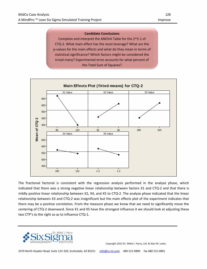
MidCo Case Analysis 126
A MindPro ™ Lean Six Sigma Simulated Training Project Improve
Copyright 2015 Dr. Mikel J. Harry, Ltd. & Alan M. Leduc
3370 North Hayden Road, Suite 123‐320, Scottsdale, AZ 85251 info@ss‐mi.com 480 515‐0890 fax 480 515‐0891
Mea
n of
CTQ
-2
12080
650
600
550
500
450
3630 320280
110100
650
600
550
500
450
1.31.2
X1 Value X2 Value X3 Value
X4 Value X5 Value
Main Effects Plot (fitted means) for CTQ-2
The fractional factorial is consistent with the regression analysis performed in the analyze phase, which
indicated that there was a strong negative linear relationship between factors X1 and CTQ‐2 and that there is
mildly positive linear relationship between X2, X4, and X5 to CTQ‐2. The analyze phase indicated that the linear
relationship between X3 and CTQ‐2 was insignificant but the main effects plot of the experiment indicates that
there may be a positive correlation. From the measure phase we know that we need to significantly move the
centering of CTQ‐2 downward. Since X1 and X5 have the strongest influence it we should look at adjusting these
two CTP’s to the right so as to influence CTQ‐1.
Candidate Conclusions
Complete and interpret the ANOVA Table for the 2^5‐1 of
CTQ‐2. What main effect has the most leverage? What are the
p‐values for the main effects and what do they mean in terms of
statistical significance? Which factors might be considered the
trivial many? Experimental error accounts for what percent of
the Total Sum of Squares?
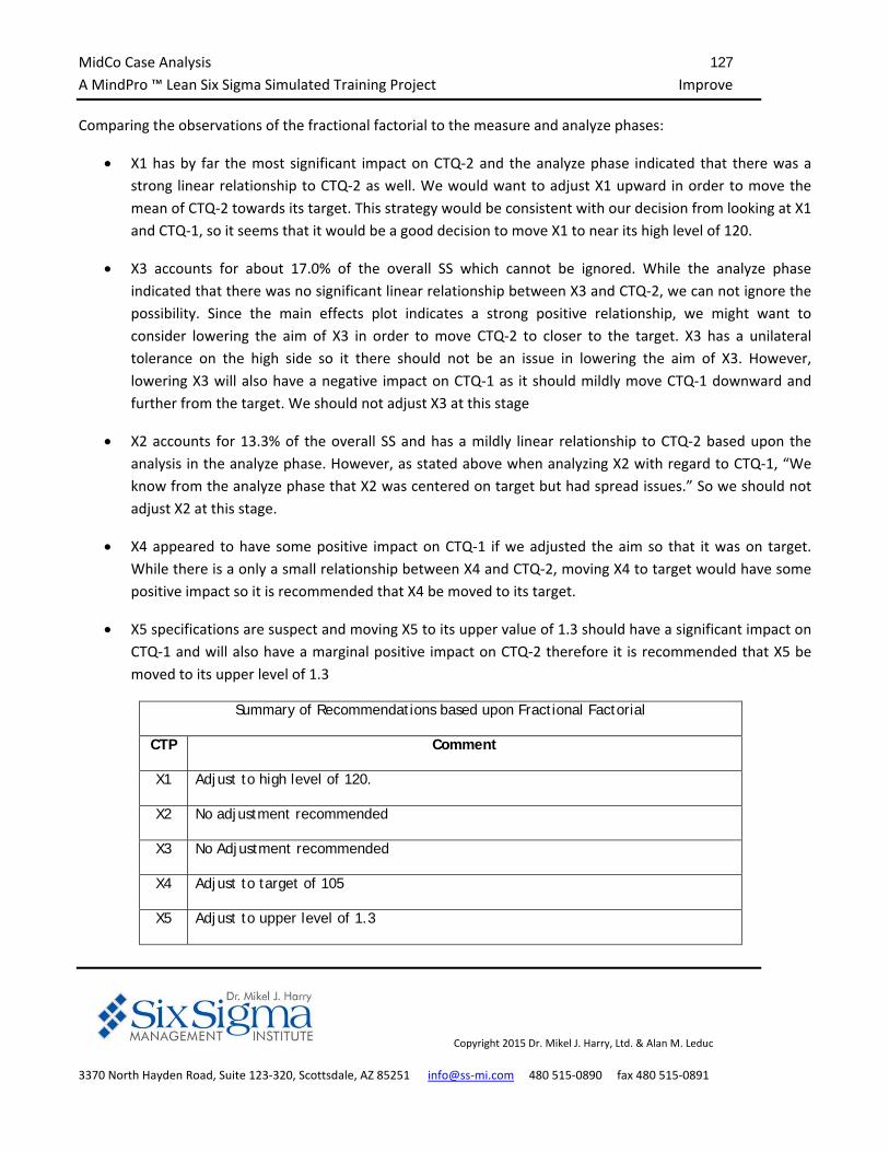
MidCo Case Analysis 127
A MindPro ™ Lean Six Sigma Simulated Training Project Improve
Copyright 2015 Dr. Mikel J. Harry, Ltd. & Alan M. Leduc
3370 North Hayden Road, Suite 123‐320, Scottsdale, AZ 85251 info@ss‐mi.com 480 515‐0890 fax 480 515‐0891
Comparing the observations of the fractional factorial to the measure and analyze phases:
X1 has by far the most significant impact on CTQ‐2 and the analyze phase indicated that there was a
strong linear relationship to CTQ‐2 as well. We would want to adjust X1 upward in order to move the
mean of CTQ‐2 towards its target. This strategy would be consistent with our decision from looking at X1
and CTQ‐1, so it seems that it would be a good decision to move X1 to near its high level of 120.
X3 accounts for about 17.0% of the overall SS which cannot be ignored. While the analyze phase
indicated that there was no significant linear relationship between X3 and CTQ‐2, we can not ignore the
possibility. Since the main effects plot indicates a strong positive relationship, we might want to
consider lowering the aim of X3 in order to move CTQ‐2 to closer to the target. X3 has a unilateral
tolerance on the high side so it there should not be an issue in lowering the aim of X3. However,
lowering X3 will also have a negative impact on CTQ‐1 as it should mildly move CTQ‐1 downward and
further from the target. We should not adjust X3 at this stage
X2 accounts for 13.3% of the overall SS and has a mildly linear relationship to CTQ‐2 based upon the
analysis in the analyze phase. However, as stated above when analyzing X2 with regard to CTQ‐1, “We
know from the analyze phase that X2 was centered on target but had spread issues.” So we should not
adjust X2 at this stage.
X4 appeared to have some positive impact on CTQ‐1 if we adjusted the aim so that it was on target.
While there is a only a small relationship between X4 and CTQ‐2, moving X4 to target would have some
positive impact so it is recommended that X4 be moved to its target.
X5 specifications are suspect and moving X5 to its upper value of 1.3 should have a significant impact on
CTQ‐1 and will also have a marginal positive impact on CTQ‐2 therefore it is recommended that X5 be
moved to its upper level of 1.3
Summary of Recommendations based upon Fractional Factorial
CTP Comment
X1 Adjust to high level of 120.
X2 No adjustment recommended
X3 No Adjustment recommended
X4 Adjust to target of 105
X5 Adjust to upper level of 1.3
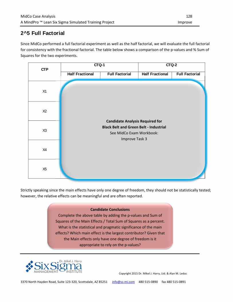
MidCo Case Analysis 128
A MindPro ™ Lean Six Sigma Simulated Training Project Improve
Copyright 2015 Dr. Mikel J. Harry, Ltd. & Alan M. Leduc
3370 North Hayden Road, Suite 123‐320, Scottsdale, AZ 85251 info@ss‐mi.com 480 515‐0890 fax 480 515‐0891
2^5 Full Factorial
Since MidCo performed a full factorial experiment as well as the half factorial, we will evaluate the full factorial
for consistency with the fractional factorial. The table below shows a comparison of the p‐values and % Sum of
Squares for the two experiments.
CTP CTQ-1 CTQ-2
Half Fractional Full Factorial Half Fractional Full Factorial
X1
0.000 27.2%
0.000 27.2%
0.000 64.3%
0.000 64.3%
X2
0.009 5.7%
0.000 5.7%
0.000 13.3%
0.000 13.3%
X3
0.110 1.7%
0.009 1.7%
0.000 17.0%
0.000 17.0%
X4
0.012 5.1%
0.000 5.2%
0.026 1.0%
0.000 1.1%
X5
0.000 54.9%
0.000 54.8%
0.002 2.8%
0.000 2.8%
Strictly speaking since the main effects have only one degree of freedom, they should not be statistically tested;
however, the relative effects can be meaningful and are often reported.
Candidate Analysis Required for
Black Belt and Green Belt ‐ Industrial
See MidCo Exam Workbook:
Improve Task 3
Candidate Conclusions
Complete the above table by adding the p‐values and Sum of
Squares of the Main Effects / Total Sum of Squares as a percent.
What is the statistical and pragmatic significance of the main
effects? Which main effect is the largest contributor? Given that
the Main effects only have one degree of freedom is it
appropriate to rely on the p‐values?
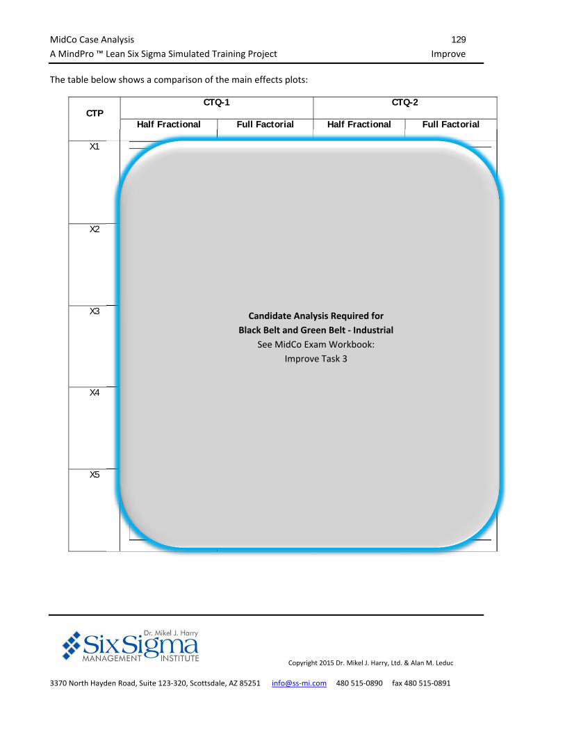
MidCo Case Analysis 129
A MindPro ™ Lean Six Sigma Simulated Training Project Improve
Copyright 2015 Dr. Mikel J. Harry, Ltd. & Alan M. Leduc
3370 North Hayden Road, Suite 123‐320, Scottsdale, AZ 85251 info@ss‐mi.com 480 515‐0890 fax 480 515‐0891
The table below shows a comparison of the main effects plots:
CTP CTQ-1 CTQ-2
Half Fractional Full Factorial Half Fractional Full Factorial
X1
X2
X3
X4
X5
Candidate Analysis Required for
Black Belt and Green Belt ‐ Industrial
See MidCo Exam Workbook:
Improve Task 3
MidCo Case Analysis 130
A MindPro ™ Lean Six Sigma Simulated Training Project Improve
Copyright 2015 Dr. Mikel J. Harry, Ltd. & Alan M. Leduc
3370 North Hayden Road, Suite 123‐320, Scottsdale, AZ 85251 info@ss‐mi.com 480 515‐0890 fax 480 515‐0891
The data from the full factorial is consistent with the half factorial, maybe too consistent. MidCo was contacted
and queried as to the process utilized for the experiment. We had a concern that the data was so consistent that
it might be a manipulation. MidCo assured us that their processes were spot on and that they had been properly
randomized. They further assured us that they had done two separate experiments. Given the consistency of the
data, the full factorial will be used for analysis from this point forward and the conclusions drawn from the half
factorial will stand.
Candidate Conclusions
Complete the above table by adding the Main Effects Plots.
Which main effects appear to have the most leverage? Which
main effects have positive slopes? Negative slopes? Which main
effects appear that they may simply be a result of chance
sampling variation? What is the meaning of the steepness of the
slope in terms of evaluating influence on the CTQ?
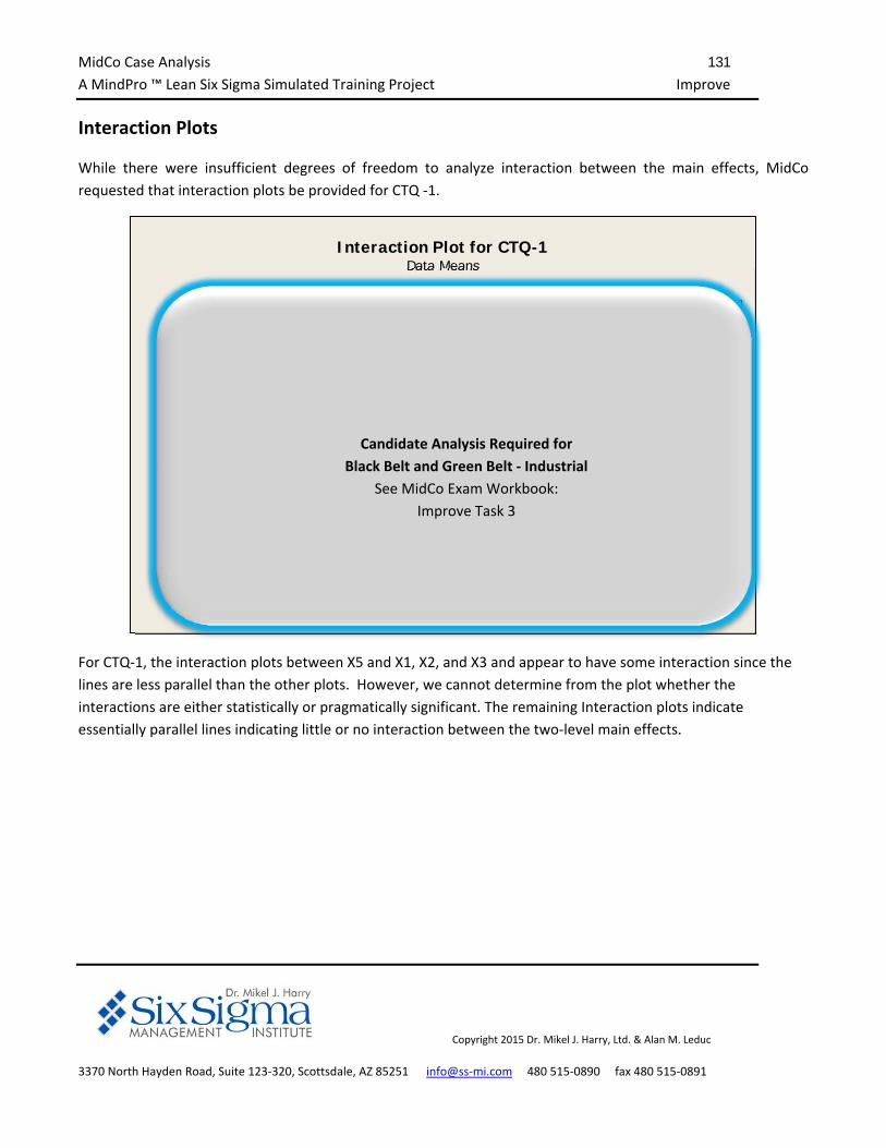
MidCo Case Analysis 131
A MindPro ™ Lean Six Sigma Simulated Training Project Improve
Copyright 2015 Dr. Mikel J. Harry, Ltd. & Alan M. Leduc
3370 North Hayden Road, Suite 123‐320, Scottsdale, AZ 85251 info@ss‐mi.com 480 515‐0890 fax 480 515‐0891
Interaction Plots
While there were insufficient degrees of freedom to analyze interaction between the main effects, MidCo
requested that interaction plots be provided for CTQ ‐1.
36.030.0 320.0280.0 110.000100.000 1.31.1100
75
50
100
75
50
100
75
50
100
75
50
X1 Value
X2 Value
X3 Value
X4 Value
X5 Value
80.0120.0
X1 Value
30.036.0
X2 Value
280.0320.0
X3 Value
100.000110.000
X4 Value
Interaction Plot for CTQ-1Data Means
For CTQ‐1, the interaction plots between X5 and X1, X2, and X3 and appear to have some interaction since the
lines are less parallel than the other plots. However, we cannot determine from the plot whether the
interactions are either statistically or pragmatically significant. The remaining Interaction plots indicate
essentially parallel lines indicating little or no interaction between the two‐level main effects.
Candidate Analysis Required for
Black Belt and Green Belt ‐ Industrial
See MidCo Exam Workbook:
Improve Task 3
MidCo Case Analysis 132
A MindPro ™ Lean Six Sigma Simulated Training Project Improve
Copyright 2015 Dr. Mikel J. Harry, Ltd. & Alan M. Leduc
3370 North Hayden Road, Suite 123‐320, Scottsdale, AZ 85251 info@ss‐mi.com 480 515‐0890 fax 480 515‐0891
36.030.0 320.0280.0 110.000100.000 1.31.1750
600
450750
600
450
750
600
450750
600
450
X1 Value
X2 Value
X3 Value
X4 Value
X5 Value
80.0120.0
X1 Value
30.036.0
X2 Value
280.0320.0
X3 Value
100.000110.000
X4 Value
Interaction Plot for CTQ-2Data Means
Candidate Conclusions
Develop interaction plots for all main effects.
Interpret when one factor is held low, how does this impact the
influence on the CTQ when comparing another factor at its low
and high setting? What is the meaning of parallel lines? What is
the meaning of non‐parallel lines? Do the interaction plots tell
the analyst whether or not the data is statistically or practically
significant? Which plots indicate a likely interaction?
Candidate Analysis Required for
Black Belt and Green Belt ‐ Industrial
See MidCo Exam Workbook:
Improve Task 3
Candidate Analysis Required for
Black Belt and Green Belt ‐ Industrial
See MidCo Exam Workbook:
Improve Task 3
MidCo Case Analysis 133
A MindPro ™ Lean Six Sigma Simulated Training Project Improve
Copyright 2015 Dr. Mikel J. Harry, Ltd. & Alan M. Leduc
3370 North Hayden Road, Suite 123‐320, Scottsdale, AZ 85251 info@ss‐mi.com 480 515‐0890 fax 480 515‐0891
MidCo continued to press on the issues of interactions, so the Full Factorial ANOVA was redone using a full
model which included all interactions. There were insufficient degrees of freedom to provide any p‐values but
at least the relative Sum of Square could be evaluated.
Folded Designs
CTQ‐1
Due to the minimal effect of X3 Value on CTQ‐1, it was decided to run an ANOVA which would fold X3 Value into
the design. The ANOVA table for the folded design is show below:
Source DF Seq SS Adj SS Adj MS F P X1 Value 1 5681.8 5681.8 5681.8 211.30 0.000 X2 Value 1 1188.3 1188.3 1188.3 44.19 0.000 X4 Value 1 1085.8 1085.8 1085.8 40.38 0.000 X5 Value 1 11445.8 11445.8 11445.8 425.65 0.000 X1 Value*X2 Value 1 69.0 69.0 69.0 2.57 0.129 X1 Value*X4 Value 1 1.3 1.3 1.3 0.05 0.830 X1 Value*X5 Value 1 812.0 812.0 812.0 30.20 0.000 X2 Value*X4 Value 1 0.3 0.3 0.3 0.01 0.920 X2 Value*X5 Value 1 170.2 170.2 170.2 6.33 0.023 X4 Value*X5 Value 1 3.1 3.1 3.1 0.12 0.738 X1 Value*X2 Value*X4 Value 1 0.0 0.0 0.0 0.00 0.984 X1 Value*X2 Value*X5 Value 1 11.8 11.8 11.8 0.44 0.518 X1 Value*X4 Value*X5 Value 1 0.2 0.2 0.2 0.01 0.925 X2 Value*X4 Value*X5 Value 1 0.0 0.0 0.0 0.00 0.973 X1 Value*X2 Value*X4 Value*X5 Value 1 0.0 0.0 0.0 0.00 0.995 Error 16 430.2 430.2 26.9 Total 31 20899.9 S = 5.18556 R-Sq = 97.94% R-Sq(adj) = 96.01%
Candidate Conclusions
Perform a Full Factorial with a full model which includes all
interactions. What is the influence of higher order interactions
in comparison to lower order interactions? Which two level
interactions have the most influence?
Candidate Analysis Required for
Black Belt and Green Belt ‐ Industrial
See MidCo Exam Workbook:
Improve Task 4
MidCo Case Analysis 134
A MindPro ™ Lean Six Sigma Simulated Training Project Improve
Copyright 2015 Dr. Mikel J. Harry, Ltd. & Alan M. Leduc
3370 North Hayden Road, Suite 123‐320, Scottsdale, AZ 85251 info@ss‐mi.com 480 515‐0890 fax 480 515‐0891
We can see that by folding X3 Value, that the other main effects are statistically significant at the below the 0.001 level. However, factors X2 Value and X4 Value have very little effect on CTQ‐1. Therefore it was decided that we would also fold X2 and X3 Value into the design. The resulting ANOVA table is show below:
Source DF Seq SS Adj SS Adj MS F P X1 Value 1 5681.8 5681.8 5681.8 53.74 0.000 X5 Value 1 11445.8 11445.8 11445.8 108.26 0.000 X1 Value*X5 Value 1 812.0 812.0 812.0 7.68 0.010 Error 28 2960.3 2960.3 105.7 Total 31 20899.9 S = 10.2822 R-Sq = 85.84% R-Sq(adj) = 84.32%
When we fold the design we simply remove the Sum of Squares from the removed factors from the model and those sum of squares then get added to the error term. The effect of folding the design is increasing the number of replications for the factors that are not removed from the design.
Candidate Conclusions
Complete the ANOVA table. When starting with a 2^5 Factorial
Design, what type of design do you have when you fold in a
single factor, i.e. 2^What Exponent? How many runs? How many
replicates? Which of the remaining main effects are statistically
significant in the folded design? Which of the interactions are
statistically significant in the folded design?
Candidate Analysis Required for
Black Belt and Green Belt ‐ Industrial
See MidCo Exam Workbook:
Improve Task 5
Candidate Conclusions
Complete the ANOVA table. When starting with a 2^5 Factorial
Design, what type of design do you have when you fold in a
three factors, i.e. 2^What Exponent? How many runs? How
many replicates? Which of the remaining main effects are
statistically significant in the folded design? Is the interaction
statistically significant in the folded design? How do the sum of
squares for the remaining effects in the folded designs and the
total sum of squares compare to the Full Factorial design before
folding?
MidCo Case Analysis 135
A MindPro ™ Lean Six Sigma Simulated Training Project Improve
Copyright 2015 Dr. Mikel J. Harry, Ltd. & Alan M. Leduc
3370 North Hayden Road, Suite 123‐320, Scottsdale, AZ 85251 info@ss‐mi.com 480 515‐0890 fax 480 515‐0891
CTQ‐2
For CTQ‐2, X4 Values and X5 Values had the least effect so it was decided that they should be folded into the
design. The resulting ANOVA table is show below:
Source DF Seq SS Adj SS Adj MS F P X1 Value 1 400513 400513 400513 379.64 0.000 X2 Value 1 82825 82825 82825 78.51 0.000 X3 Value 1 105570 105570 105570 100.07 0.000 X1 Value*X2 Value 1 3321 3321 3321 3.15 0.089 X1 Value*X3 Value 1 4232 4232 4232 4.01 0.057 X2 Value*X3 Value 1 882 882 882 0.84 0.370 X1 Value*X2 Value*X3 Value 1 36 36 36 0.03 0.855 Error 24 25319 25319 1055 Total 31 622698 S = 32.4804 R-Sq = 95.93% R-Sq(adj) = 94.75%
As with CTQ‐1, the folded design reveals that all of the remaining main effects are statistically significant below
0.001.
Candidate Analysis Required for
Black Belt and Green Belt ‐ Industrial
See MidCo Exam Workbook:
Improve Task 6
Candidate Conclusions
Complete the ANOVA table. When starting with a 2^5 Factorial
Design, what type of design do you have when you fold in a two
factors, i.e. 2^What Exponent? How many runs? How many
replicates? Which of the remaining main effects are statistically
significant in the folded design? Which interactions are
statistically significant in the folded design? What is the practical
significance of the main effects and interactions?
MidCo Case Analysis 136
A MindPro ™ Lean Six Sigma Simulated Training Project Improve
Copyright 2015 Dr. Mikel J. Harry, Ltd. & Alan M. Leduc
3370 North Hayden Road, Suite 123‐320, Scottsdale, AZ 85251 info@ss‐mi.com 480 515‐0890 fax 480 515‐0891
Distribution of CTQ’s
After the analysis was complete, the question came up in discussions with MidCo with regard to the distribution
of the CTQ‐1 and CTQ‐2 data. As a result a histogram and normal probability plot was performed on the CTQ’s
as show below:
120100806040200
6
5
4
3
2
1
0
CTQ-1
Freq
uenc
y
Mean 60.07StDev 25.97N 32
Histogram of CTQ-1Normal
120100806040200
99
95
90
80
70
60504030
20
10
5
1
CTQ-1Pe
rcen
t
Mean 60.07StDev 25.97N 32AD 0.668P-Value 0.074
Probability Plot of CTQ-1Normal
840720600480360240
6
5
4
3
2
1
0
CTQ-2
Freq
uenc
y
Mean 559.6StDev 141.7N 32
Histogram of CTQ-2Normal
900800700600500400300200
99
95
90
80
70
60504030
20
10
5
1
CTQ-2
Perc
ent
Mean 559.6StDev 141.7N 32AD 0.313P-Value 0.531
Probability Plot of CTQ-2Normal
Generally 100 or more observations are considered adequate when using histograms to identify distributions. In
this case we only have 32 runs so it is not surprising the histogram does not have the typical bell shaped curve. It
is best in these situations to perform a normal probability plot with and Andersen Darling Test.
Candidate Analysis Required for
Black Belt and Green Belt ‐ Industrial
See MidCo Exam Workbook:
Improve Task 7
Candidate Analysis Required for
Black Belt and Green Belt ‐ Industrial
See MidCo Exam Workbook:
Improve Task 7
Candidate Conclusions
Develop the above graphs.
Does the data appear to be normally distributed?
How does CTQ‐1 compare to CTQ‐2 in terms of normality?
Candidate Analysis Required for
Black Belt and Green Belt ‐ Industrial
See MidCo Exam Workbook:
Improve Task 7
Candidate Analysis Required for
Black Belt and Green Belt ‐ Industrial
See MidCo Exam Workbook:
Improve Task 7
MidCo Case Analysis 137
A MindPro ™ Lean Six Sigma Simulated Training Project Improve
Copyright 2015 Dr. Mikel J. Harry, Ltd. & Alan M. Leduc
3370 North Hayden Road, Suite 123‐320, Scottsdale, AZ 85251 info@ss‐mi.com 480 515‐0890 fax 480 515‐0891
Additional Analysis
Although MidCo’s Half‐Fractional and Full Factorial were analyzed thoroughly, a request was made for some
additional analysis:
MidCo ask that an F‐test be performed to determine if there was a difference in the variances of CTQ‐1
for the group where X1 Value was set low versus when X1 Value was set high.
X1 Value N StDev Variance 80.0 16 16.515 272.731 120.0 16 27.236 741.813
MidCo ask that an F‐test be performed to determine if there was a difference in the variances of CTQ‐1
for the group where X2 Value was set low versus when X2 Value was set high.
X2 Value N StDev Variance 30.0 16 28.334 802.821 36.0 16 22.612 511.290
Candidate Analysis Required for
Black Belt, Green Belt – Industrial and Green Belt Commercial
See MidCo Exam Workbook:
Improve Task 8
Candidate Conclusions
Is the variance of X2 Value when set low versus when set high
difference with respect to CTQ‐1
Candidate Analysis Required for
Black Belt, Green Belt – Industrial and Green Belt Commercial
See MidCo Exam Workbook:
Improve Task 8
Candidate Conclusions
Is the variance of X1 Value when set low versus when set high
difference with respect to CTQ‐1
MidCo Case Analysis 138
A MindPro ™ Lean Six Sigma Simulated Training Project Improve
Copyright 2015 Dr. Mikel J. Harry, Ltd. & Alan M. Leduc
3370 North Hayden Road, Suite 123‐320, Scottsdale, AZ 85251 info@ss‐mi.com 480 515‐0890 fax 480 515‐0891
MidCo ask that an t‐test be performed to determine if there was a difference in the means of CTQ‐1 for
the group where X1 Value was set low versus when X1 Value was set high.
X1 Value N Mean StDev SE Mean 80.0 16 46.8 16.5 4.1 120.0 16 73.4 27.2 6.8
MidCo ask that a t‐test be performed to determine if there was a difference in the means of CTQ‐1 for
the group where X2 Value was set low versus when X2 Value was set high.
X2 Value N Mean StDev SE Mean 30.0 16 66.2 28.3 7.1 36.0 16 54.0 22.6 5.7
Candidate Conclusions
Is the Mean of X1 Value when set low versus when set high
difference with respect to CTQ‐1
Candidate Conclusions
Is the Mean of X2 Value when set low versus when set high
difference with respect to CTQ‐1
Candidate Analysis Required for
Black Belt, Green Belt – Industrial and Green Belt Commercial
See MidCo Exam Workbook:
Improve Task 8
Candidate Analysis Required for
Black Belt, Green Belt – Industrial and Green Belt Commercial
See MidCo Exam Workbook:
Improve Task 8
MidCo Case Analysis 139
A MindPro ™ Lean Six Sigma Simulated Training Project Improve
Copyright 2015 Dr. Mikel J. Harry, Ltd. & Alan M. Leduc
3370 North Hayden Road, Suite 123‐320, Scottsdale, AZ 85251 info@ss‐mi.com 480 515‐0890 fax 480 515‐0891
Midco wanted to see a Multi‐Vari Chart on CTQ‐1 with respect to Variables X1 Value, X2 Value, and X5
Value and on CTQ‐2 with respect to Variables X1 Value, X2 Value, and X3 Value.
36.030.0
110
100
90
80
70
60
50
40
30
20
36.030.0
1.150
X2 Value
CTQ
-1
1.25080.0
120.0
X1 Value
Multi-Vari Chart for CTQ-1 by X1 Value - X5 Value
Panel variable: X5 Value
36.030.0
800
700
600
500
400
300
36.030.0
280.0
X2 Value
CTQ
-2
320.080.0
120.0
X1 Value
Multi-Vari Chart for CTQ-2 by X1 Value - X3 Value
Panel variable: X3 Value
Candidate Analysis Required for
Black Belt, Green Belt – Industrial
and Green Belt Commercial
See MidCo Exam Workbook:
Improve Task 9
Candidate Conclusions
Does the dominant source of variation in CTQ‐1 appear to be
from X1 Value, X2 Value or X5 Value? Does the dominant source
of variation in CTQ‐2 appear to be from X1 Value, X2 Value or X3
Value?
Candidate Analysis Required for
Black Belt, Green Belt – Industrial
and Green Belt Commercial
See MidCo Exam Workbook:
Improve Task 9
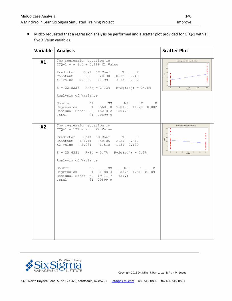
MidCo Case Analysis 140
A MindPro ™ Lean Six Sigma Simulated Training Project Improve
Copyright 2015 Dr. Mikel J. Harry, Ltd. & Alan M. Leduc
3370 North Hayden Road, Suite 123‐320, Scottsdale, AZ 85251 info@ss‐mi.com 480 515‐0890 fax 480 515‐0891
Midco requested that a regression analysis be performed and a scatter plot provided for CTQ‐1 with all
five X Value variables.
Variable Analysis Scatter Plot
X1 The regression equation is CTQ-1 = - 6.5 + 0.666 X1 Value Predictor Coef SE Coef T P Constant -6.55 20.30 -0.32 0.749 X1 Value 0.6662 0.1991 3.35 0.002 S = 22.5227 R-Sq = 27.2% R-Sq(adj) = 24.8% Analysis of Variance Source DF SS MS F P Regression 1 5681.8 5681.8 11.20 0.002 Residual Error 30 15218.2 507.3 Total 31 20899.9
1201101009080
120
100
80
60
40
20
X1 Value
CTQ
-1
Scatterplot of CTQ-1 vs X1 Value
X2 The regression equation is CTQ-1 = 127 - 2.03 X2 Value Predictor Coef SE Coef T P Constant 127.11 50.05 2.54 0.017 X2 Value -2.031 1.510 -1.34 0.189 S = 25.6331 R-Sq = 5.7% R-Sq(adj) = 2.5% Analysis of Variance Source DF SS MS F P Regression 1 1188.3 1188.3 1.81 0.189 Residual Error 30 19711.7 657.1 Total 31 20899.9
36353433323130
120
100
80
60
40
20
X2 Value
CTQ
-1
Scatterplot of CTQ-1 vs X2 Value
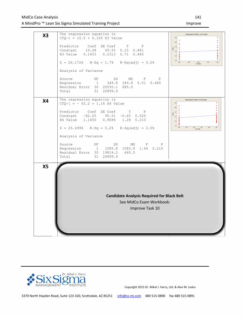
MidCo Case Analysis 141
A MindPro ™ Lean Six Sigma Simulated Training Project Improve
Copyright 2015 Dr. Mikel J. Harry, Ltd. & Alan M. Leduc
3370 North Hayden Road, Suite 123‐320, Scottsdale, AZ 85251 info@ss‐mi.com 480 515‐0890 fax 480 515‐0891
X3 The regression equation is CTQ-1 = 10.5 + 0.165 X3 Value Predictor Coef SE Coef T P Constant 10.48 69.55 0.15 0.881 X3 Value 0.1653 0.2313 0.71 0.480 S = 26.1726 R-Sq = 1.7% R-Sq(adj) = 0.0% Analysis of Variance Source DF SS MS F P Regression 1 349.8 349.8 0.51 0.480 Residual Error 30 20550.1 685.0 Total 31 20899.9
320310300290280
120
100
80
60
40
20
X3 Value
CTQ
-1
Scatterplot of CTQ-1 vs X3 Value
X4 The regression equation is CTQ-1 = - 62.2 + 1.16 X4 Value Predictor Coef SE Coef T P Constant -62.25 95.51 -0.65 0.520 X4 Value 1.1650 0.9086 1.28 0.210 S = 25.6996 R-Sq = 5.2% R-Sq(adj) = 2.0% Analysis of Variance Source DF SS MS F P Regression 1 1085.8 1085.8 1.64 0.210 Residual Error 30 19814.2 660.5 Total 31 20899.9
110108106104102100
120
100
80
60
40
20
X4 Value
CTQ
-1
Scatterplot of CTQ-1 vs X4 Value
X5 The regression equation is CTQ-1 = - 394 + 378 X5 Value Predictor Coef SE Coef T P Constant -393.82 75.38 -5.22 0.000 X5 Value 378.25 62.76 6.03 0.000 S = 17.7521 R-Sq = 54.8% R-Sq(adj) = 53.3% Analysis of Variance Source DF SS MS F P Regression 1 11446 11446 36.32 0.000 Residual Error 30 9454 315 Total 31 20900
1.2501.2251.2001.1751.150
120
100
80
60
40
20
X5 Value
CTQ
-1
Scatterplot of CTQ-1 vs X5 Value
Candidate Analysis Required for Black Belt
See MidCo Exam Workbook:
Improve Task 10
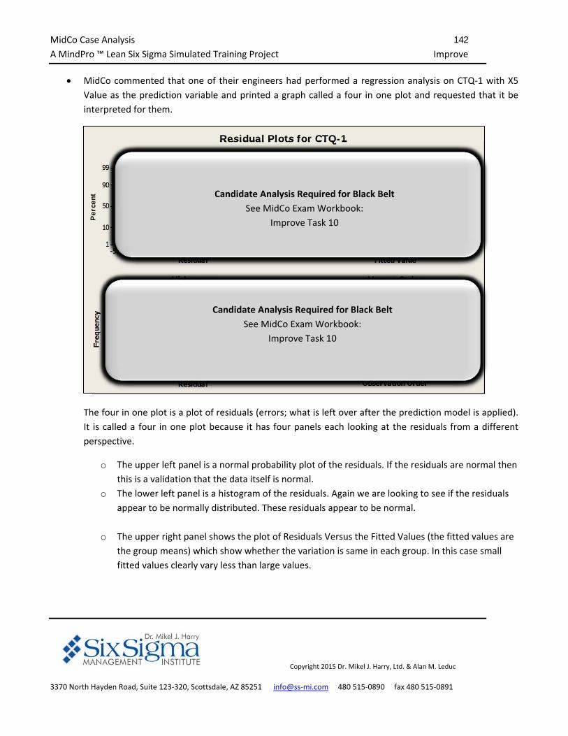
MidCo Case Analysis 142
A MindPro ™ Lean Six Sigma Simulated Training Project Improve
Copyright 2015 Dr. Mikel J. Harry, Ltd. & Alan M. Leduc
3370 North Hayden Road, Suite 123‐320, Scottsdale, AZ 85251 info@ss‐mi.com 480 515‐0890 fax 480 515‐0891
MidCo commented that one of their engineers had performed a regression analysis on CTQ‐1 with X5
Value as the prediction variable and printed a graph called a four in one plot and requested that it be
interpreted for them.
50250-25-50
99
90
50
10
1
Residual
Per
cent
8070605040
40
20
0
-20
-40
Fitted Value
Res
idua
l
403020100-10-20-30
8
6
4
2
0
Residual
Freq
uenc
y
3230282624222018161412108642
40
20
0
-20
-40
Observation Order
Res
idua
l
Normal Probability Plot Versus Fits
Histogram Versus Order
Residual Plots for CTQ-1
The four in one plot is a plot of residuals (errors; what is left over after the prediction model is applied).
It is called a four in one plot because it has four panels each looking at the residuals from a different
perspective.
o The upper left panel is a normal probability plot of the residuals. If the residuals are normal then
this is a validation that the data itself is normal.
o The lower left panel is a histogram of the residuals. Again we are looking to see if the residuals
appear to be normally distributed. These residuals appear to be normal.
o The upper right panel shows the plot of Residuals Versus the Fitted Values (the fitted values are
the group means) which show whether the variation is same in each group. In this case small
fitted values clearly vary less than large values.
Candidate Analysis Required for Black Belt
See MidCo Exam Workbook:
Improve Task 10
Candidate Analysis Required for Black Belt
See MidCo Exam Workbook:
Improve Task 10
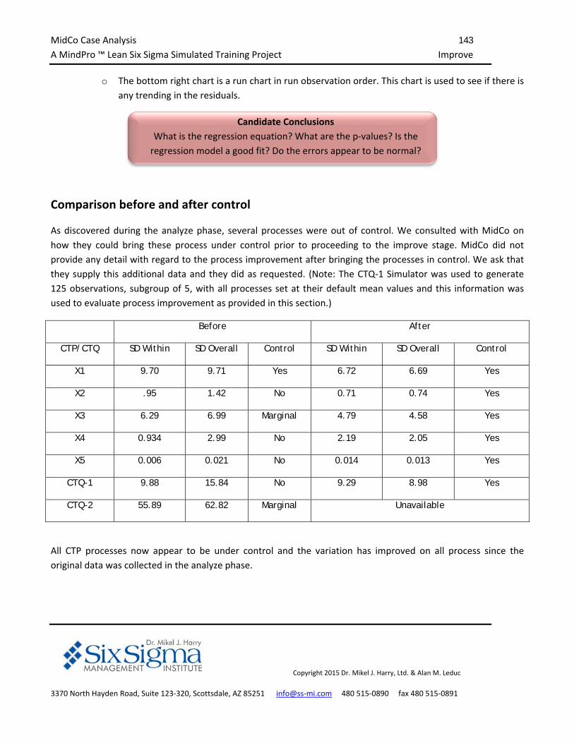
MidCo Case Analysis 143
A MindPro ™ Lean Six Sigma Simulated Training Project Improve
Copyright 2015 Dr. Mikel J. Harry, Ltd. & Alan M. Leduc
3370 North Hayden Road, Suite 123‐320, Scottsdale, AZ 85251 info@ss‐mi.com 480 515‐0890 fax 480 515‐0891
o The bottom right chart is a run chart in run observation order. This chart is used to see if there is
any trending in the residuals.
Comparison before and after control
As discovered during the analyze phase, several processes were out of control. We consulted with MidCo on
how they could bring these process under control prior to proceeding to the improve stage. MidCo did not
provide any detail with regard to the process improvement after bringing the processes in control. We ask that
they supply this additional data and they did as requested. (Note: The CTQ‐1 Simulator was used to generate
125 observations, subgroup of 5, with all processes set at their default mean values and this information was
used to evaluate process improvement as provided in this section.)
Before After
CTP/CTQ SD Within SD Overall Control SD Within SD Overall Control
X1 9.70 9.71 Yes 6.72 6.69 Yes
X2 .95 1.42 No 0.71 0.74 Yes
X3 6.29 6.99 Marginal 4.79 4.58 Yes
X4 0.934 2.99 No 2.19 2.05 Yes
X5 0.006 0.021 No 0.014 0.013 Yes
CTQ-1 9.88 15.84 No 9.29 8.98 Yes
CTQ-2 55.89 62.82 Marginal Unavailable
All CTP processes now appear to be under control and the variation has improved on all process since the
original data was collected in the analyze phase.
Candidate Conclusions
What is the regression equation? What are the p‐values? Is the
regression model a good fit? Do the errors appear to be normal?
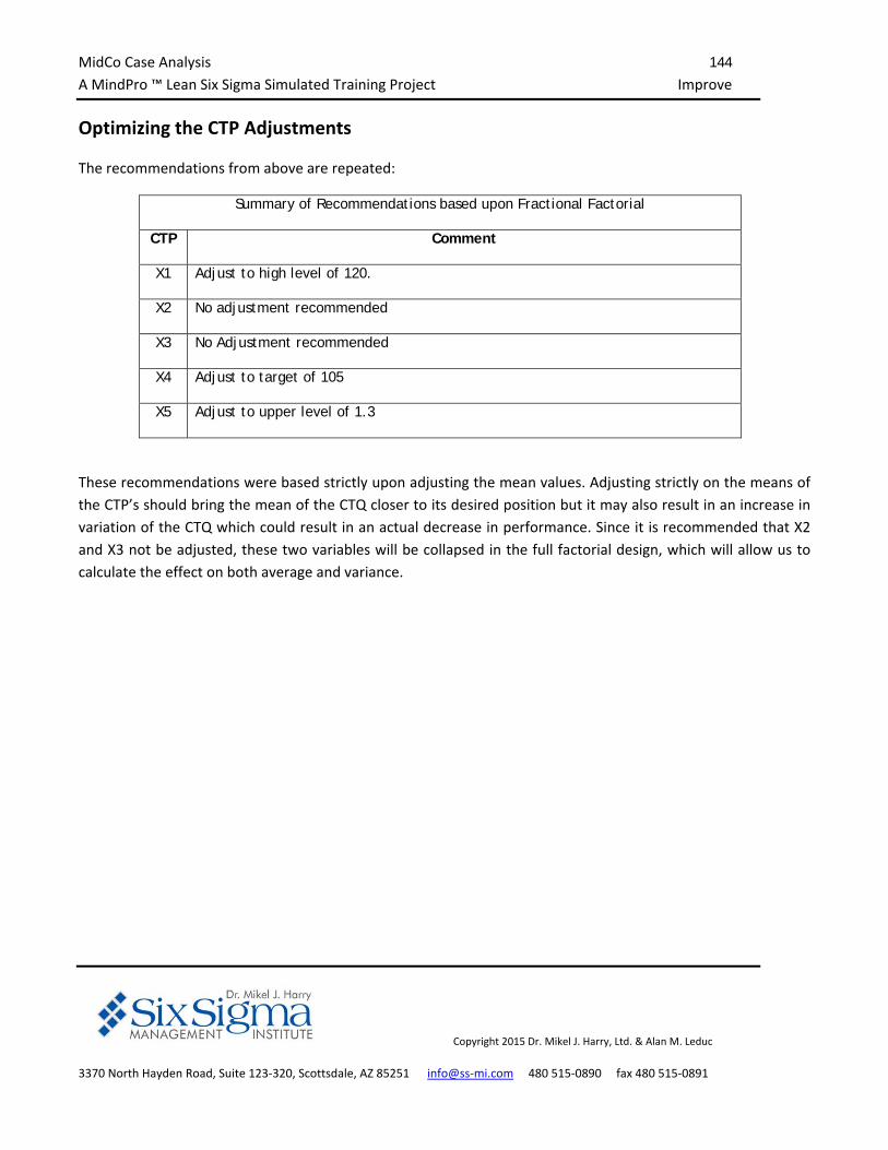
MidCo Case Analysis 144
A MindPro ™ Lean Six Sigma Simulated Training Project Improve
Copyright 2015 Dr. Mikel J. Harry, Ltd. & Alan M. Leduc
3370 North Hayden Road, Suite 123‐320, Scottsdale, AZ 85251 info@ss‐mi.com 480 515‐0890 fax 480 515‐0891
Optimizing the CTP Adjustments
The recommendations from above are repeated:
Summary of Recommendations based upon Fractional Factorial
CTP Comment
X1 Adjust to high level of 120.
X2 No adjustment recommended
X3 No Adjustment recommended
X4 Adjust to target of 105
X5 Adjust to upper level of 1.3
These recommendations were based strictly upon adjusting the mean values. Adjusting strictly on the means of
the CTP’s should bring the mean of the CTQ closer to its desired position but it may also result in an increase in
variation of the CTQ which could result in an actual decrease in performance. Since it is recommended that X2
and X3 not be adjusted, these two variables will be collapsed in the full factorial design, which will allow us to
calculate the effect on both average and variance.
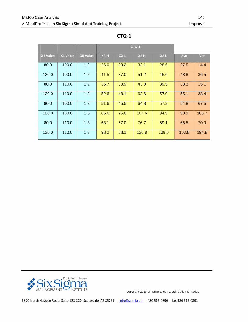
MidCo Case Analysis 145
A MindPro ™ Lean Six Sigma Simulated Training Project Improve
Copyright 2015 Dr. Mikel J. Harry, Ltd. & Alan M. Leduc
3370 North Hayden Road, Suite 123‐320, Scottsdale, AZ 85251 info@ss‐mi.com 480 515‐0890 fax 480 515‐0891
CTQ‐1
CTQ-1
X1 Value X4 Value X5 Value X3-H X3-L X2-H X2-L Avg Var
80.0 100.0 1.2 26.0 23.2 32.1 28.6 27.5 14.4
120.0 100.0 1.2 41.5 37.0 51.2 45.6 43.8 36.5
80.0 110.0 1.2 36.7 33.9 43.0 39.5 38.3 15.1
120.0 110.0 1.2 52.6 48.1 62.6 57.0 55.1 38.4
80.0 100.0 1.3 51.6 45.5 64.8 57.2 54.8 67.5
120.0 100.0 1.3 85.6 75.6 107.6 94.9 90.9 185.7
80.0 110.0 1.3 63.1 57.0 76.7 69.1 66.5 70.9
120.0 110.0 1.3 98.2 88.1 120.8 108.0 103.8 194.8
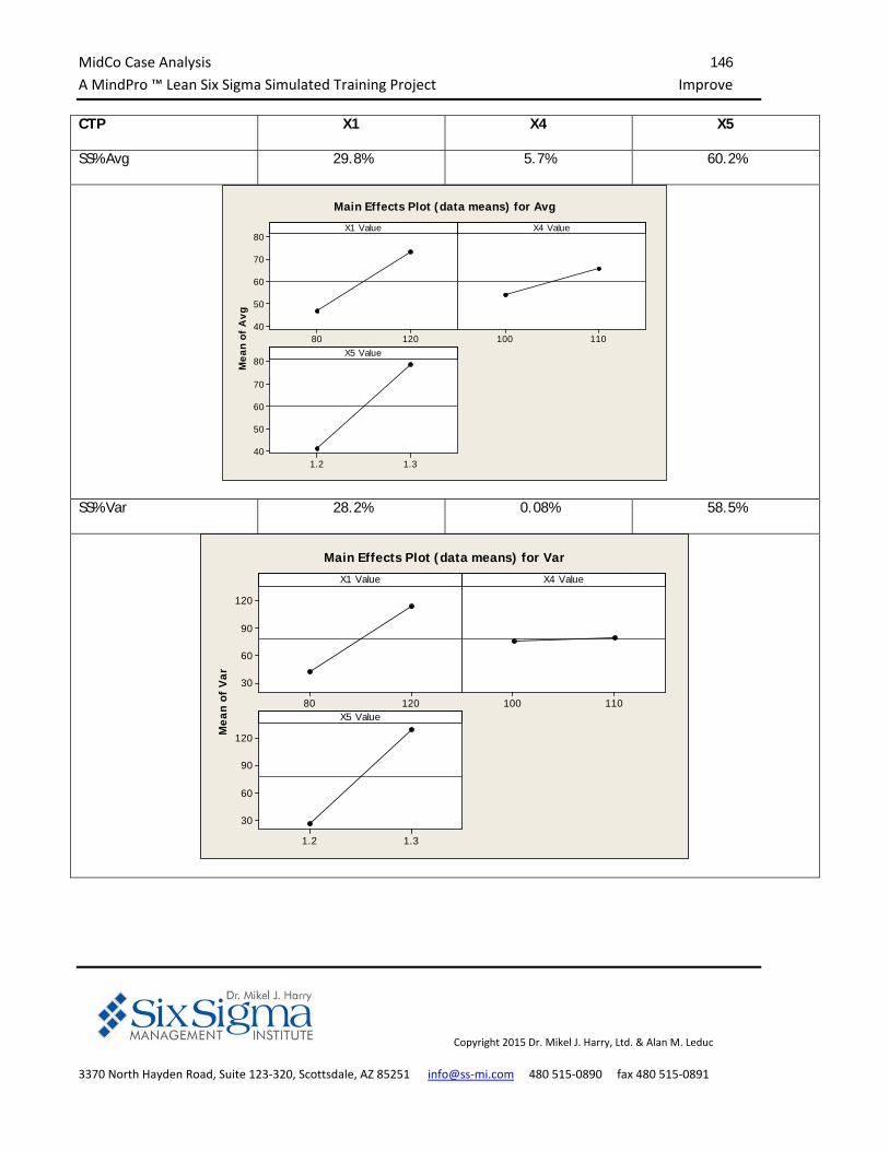
MidCo Case Analysis 146
A MindPro ™ Lean Six Sigma Simulated Training Project Improve
Copyright 2015 Dr. Mikel J. Harry, Ltd. & Alan M. Leduc
3370 North Hayden Road, Suite 123‐320, Scottsdale, AZ 85251 info@ss‐mi.com 480 515‐0890 fax 480 515‐0891
CTP X1 X4 X5
SS% Avg 29.8% 5.7% 60.2%
Mea
n of
Avg
12080
80
70
60
50
40110100
1.31.2
80
70
60
50
40
X1 Value X4 Value
X5 Value
Main Effects Plot (data means) for Avg
SS% Var 28.2% 0.08% 58.5%
Mea
n of
Var
12080
120
90
60
30
110100
1.31.2
120
90
60
30
X1 Value X4 Value
X5 Value
Main Effects Plot (data means) for Var
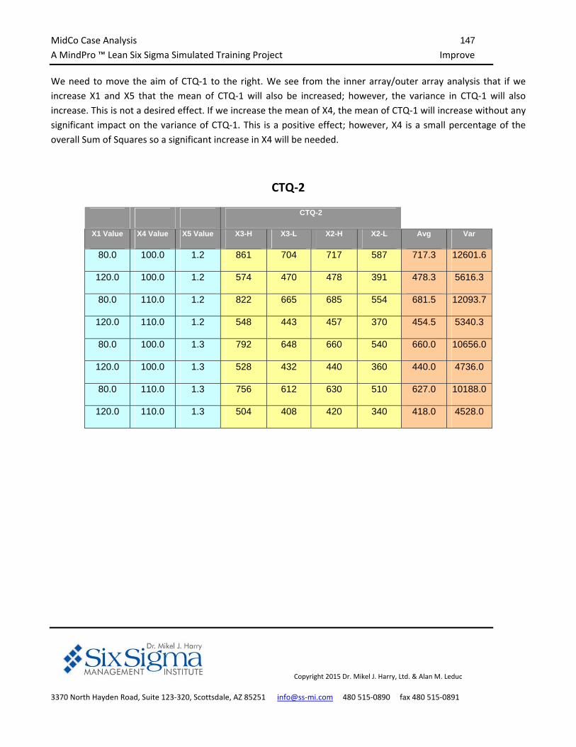
MidCo Case Analysis 147
A MindPro ™ Lean Six Sigma Simulated Training Project Improve
Copyright 2015 Dr. Mikel J. Harry, Ltd. & Alan M. Leduc
3370 North Hayden Road, Suite 123‐320, Scottsdale, AZ 85251 info@ss‐mi.com 480 515‐0890 fax 480 515‐0891
We need to move the aim of CTQ‐1 to the right. We see from the inner array/outer array analysis that if we
increase X1 and X5 that the mean of CTQ‐1 will also be increased; however, the variance in CTQ‐1 will also
increase. This is not a desired effect. If we increase the mean of X4, the mean of CTQ‐1 will increase without any
significant impact on the variance of CTQ‐1. This is a positive effect; however, X4 is a small percentage of the
overall Sum of Squares so a significant increase in X4 will be needed.
CTQ‐2
CTQ-2
X1 Value X4 Value X5 Value X3-H X3-L X2-H X2-L Avg Var
80.0 100.0 1.2 861 704 717 587 717.3 12601.6
120.0 100.0 1.2 574 470 478 391 478.3 5616.3
80.0 110.0 1.2 822 665 685 554 681.5 12093.7
120.0 110.0 1.2 548 443 457 370 454.5 5340.3
80.0 100.0 1.3 792 648 660 540 660.0 10656.0
120.0 100.0 1.3 528 432 440 360 440.0 4736.0
80.0 110.0 1.3 756 612 630 510 627.0 10188.0
120.0 110.0 1.3 504 408 420 340 418.0 4528.0
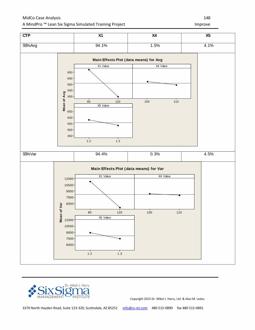
MidCo Case Analysis 148
A MindPro ™ Lean Six Sigma Simulated Training Project Improve
Copyright 2015 Dr. Mikel J. Harry, Ltd. & Alan M. Leduc
3370 North Hayden Road, Suite 123‐320, Scottsdale, AZ 85251 info@ss‐mi.com 480 515‐0890 fax 480 515‐0891
CTP X1 X4 X5
SS% Avg 94.1% 1.5% 4.1%
Mea
n of
Avg
12080
650
600
550
500
450
110100
1.31.2
650
600
550
500
450
X1 Value X4 Value
X5 Value
Main Effects Plot (data means) for Avg
SS% Var 94.4% 0.3% 4.5%
Mea
n of
Var
12080
12000
10500
9000
7500
6000
110100
1.31.2
12000
10500
9000
7500
6000
X1 Value X4 Value
X5 Value
Main Effects Plot (data means) for Var
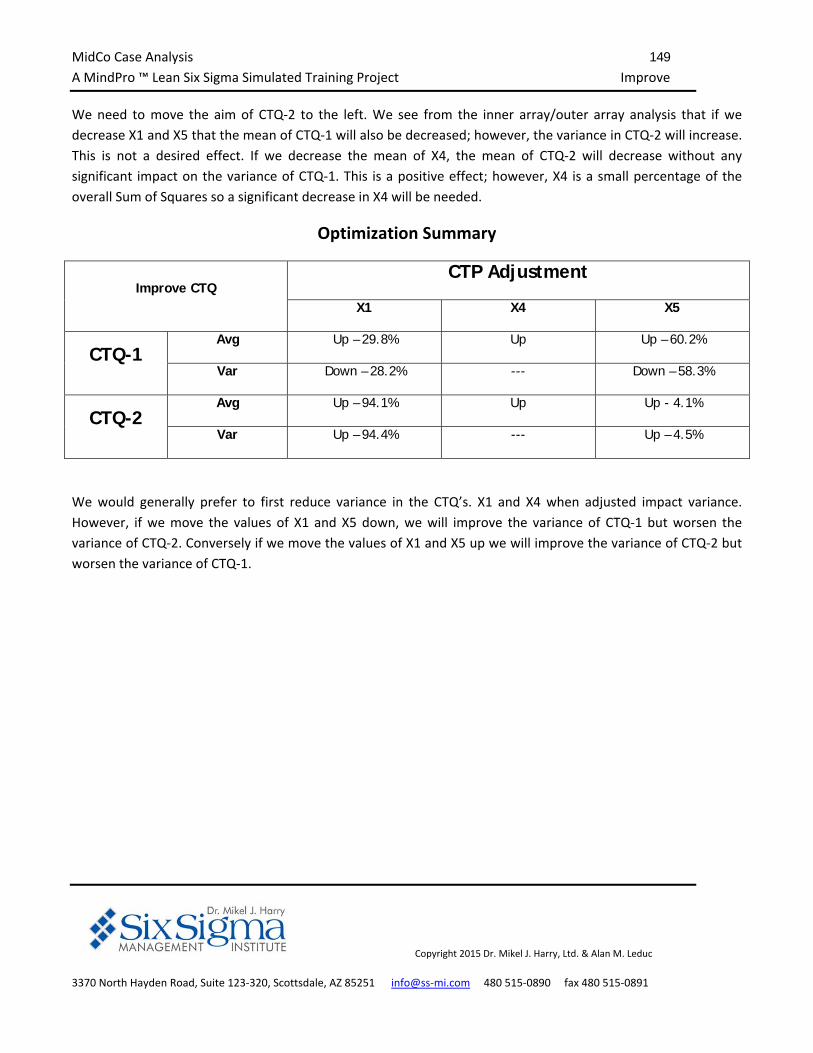
MidCo Case Analysis 149
A MindPro ™ Lean Six Sigma Simulated Training Project Improve
Copyright 2015 Dr. Mikel J. Harry, Ltd. & Alan M. Leduc
3370 North Hayden Road, Suite 123‐320, Scottsdale, AZ 85251 info@ss‐mi.com 480 515‐0890 fax 480 515‐0891
We need to move the aim of CTQ‐2 to the left. We see from the inner array/outer array analysis that if we
decrease X1 and X5 that the mean of CTQ‐1 will also be decreased; however, the variance in CTQ‐2 will increase.
This is not a desired effect. If we decrease the mean of X4, the mean of CTQ‐2 will decrease without any
significant impact on the variance of CTQ‐1. This is a positive effect; however, X4 is a small percentage of the
overall Sum of Squares so a significant decrease in X4 will be needed.
Optimization Summary
Improve CTQ CTP Adjustment
X1 X4 X5
CTQ-1 Avg Up – 29.8% Up Up – 60.2%
Var Down – 28.2% --- Down – 58.3%
CTQ-2 Avg Up – 94.1% Up Up - 4.1%
Var Up – 94.4% --- Up – 4.5%
We would generally prefer to first reduce variance in the CTQ’s. X1 and X4 when adjusted impact variance.
However, if we move the values of X1 and X5 down, we will improve the variance of CTQ‐1 but worsen the
variance of CTQ‐2. Conversely if we move the values of X1 and X5 up we will improve the variance of CTQ‐2 but
worsen the variance of CTQ‐1.
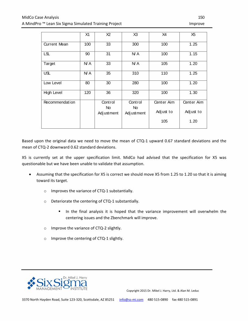
MidCo Case Analysis 150
A MindPro ™ Lean Six Sigma Simulated Training Project Improve
Copyright 2015 Dr. Mikel J. Harry, Ltd. & Alan M. Leduc
3370 North Hayden Road, Suite 123‐320, Scottsdale, AZ 85251 info@ss‐mi.com 480 515‐0890 fax 480 515‐0891
X1 X2 X3 X4 X5
Current Mean 100 33 300 100 1.25
LSL 90 31 N/A 100 1.15
Target N/A 33 N/A 105 1.20
USL N/A 35 310 110 1.25
Low Level 80 30 280 100 1.20
High Level 120 36 320 100 1.30
Recommendation Control No
Adjustment
Control No
Adjustment
Center Aim
Adjust to
105
Center Aim
Adjust to
1.20
Based upon the original data we need to move the mean of CTQ‐1 upward 0.67 standard deviations and the
mean of CTQ‐2 downward 0.62 standard deviations.
X5 is currently set at the upper specification limit. MidCo had advised that the specification for X5 was
questionable but we have been unable to validate that assumption.
Assuming that the specification for X5 is correct we should move X5 from 1.25 to 1.20 so that it is aiming
toward its target.
o Improves the variance of CTQ‐1 substantially.
o Deteriorate the centering of CTQ‐1 substantially.
In the final analysis it is hoped that the variance improvement will overwhelm the
centering issues and the Zbenchmark will improve.
o Improve the variance of CTQ‐2 slightly.
o Improve the centering of CTQ‐1 slightly.
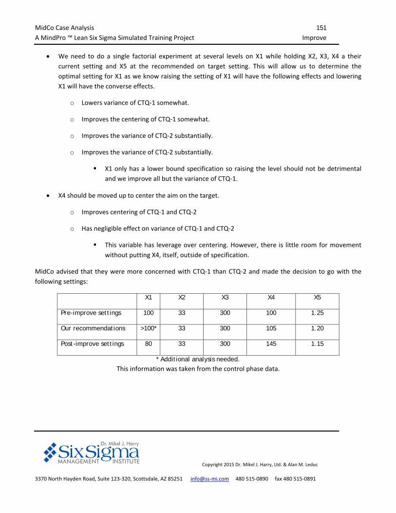
MidCo Case Analysis 151
A MindPro ™ Lean Six Sigma Simulated Training Project Improve
Copyright 2015 Dr. Mikel J. Harry, Ltd. & Alan M. Leduc
3370 North Hayden Road, Suite 123‐320, Scottsdale, AZ 85251 info@ss‐mi.com 480 515‐0890 fax 480 515‐0891
We need to do a single factorial experiment at several levels on X1 while holding X2, X3, X4 a their
current setting and X5 at the recommended on target setting. This will allow us to determine the
optimal setting for X1 as we know raising the setting of X1 will have the following effects and lowering
X1 will have the converse effects.
o Lowers variance of CTQ‐1 somewhat.
o Improves the centering of CTQ‐1 somewhat.
o Improves the variance of CTQ‐2 substantially.
o Improves the variance of CTQ‐2 substantially.
X1 only has a lower bound specification so raising the level should not be detrimental
and we improve all but the variance of CTQ‐1.
X4 should be moved up to center the aim on the target.
o Improves centering of CTQ‐1 and CTQ‐2
o Has negligible effect on variance of CTQ‐1 and CTQ‐2
This variable has leverage over centering. However, there is little room for movement
without putting X4, itself, outside of specification.
MidCo advised that they were more concerned with CTQ‐1 than CTQ‐2 and made the decision to go with the
following settings:
X1 X2 X3 X4 X5
Pre-improve settings 100 33 300 100 1.25
Our recommendations >100* 33 300 105 1.20
Post-improve settings 80 33 300 145 1.15
* Additional analysis needed.
This information was taken from the control phase data.
MidCo Case Analysis 152
A MindPro ™ Lean Six Sigma Simulated Training Project Improve
Copyright 2015 Dr. Mikel J. Harry, Ltd. & Alan M. Leduc
3370 North Hayden Road, Suite 123‐320, Scottsdale, AZ 85251 info@ss‐mi.com 480 515‐0890 fax 480 515‐0891
It appears as MidCo made the decision to ignore the impact on CTQ‐2 that will result by changing the CTP’s to
optimize CTQ‐1.
They reduced X1 and X5 which should substantially reduce the variation on CTQ‐1.
o X1 is below the specification and X5 is set to aim at the lower specification.
o The centering of CTQ‐1 should be improved but the variance of CTQ will be substantially
deteriorated.
They increased X4 which should move CTQ‐1 upward and closer to its target.
o X4 is substantially outside the specification limits.
o This will also improve the centering of CTQ‐2
MidCo has not confirmed their rationale for stepping outside the specifications on variable X1 and X4. We can
only assume that they have re‐evaluated these specifications and are in the processing of changing them. With
the adjustments, only the variance of CTQ‐2 will be negatively impacted.
MidCo Case Analysis 153
A MindPro ™ Lean Six Sigma Simulated Training Project
Copyright 2015 Dr. Mikel J. Harry, Ltd. & Alan M. Leduc
3370 North Hayden Road, Suite 123‐320, Scottsdale, AZ 85251 info@ss‐mi.com 480 515‐0890 fax 480 515‐0891
Control
What level of process control can be sustained over time?
Conclusions
As stated in the improve phase, MidCo elected to reduce the aim of X1 below the
specification. MidCo indicated that they were going to revise the specification limit of
X1 but have not done that as yet. We recommend that they revise the unilateral
specification so that the lower specification limit is 60 for a 3.14 sigma (840 ppm
defective) or 40 for a six sigma process.
X2 is properly centered but only has a 2.30 sigma value (10692 ppm defective). The
overall capability is statistically the same as the within capability so there is little if any
improvement available in the process. In order to improve X2, we will have to have a
breakthrough in the process which will likely require improved technology.
X3 is operating at 2.55 sigma (5391 ppm defective). The overall capability is statistically
the same as the within capability so like X2 in order to improve X3, a process
breakthrough likely requiring new technology will be required.
X4 like X1 has specification issues. MidCo decided to leverage X4 by moving the process
upward significantly in order to improve the variance of CTQ‐1. MidCo advised that
they were going to change the specifications but have not done that yet. If MidCo
moves the target of X4 to 145 and maintains the tolerance of +/‐5, the process will still
only be at 1.86 sigma (31170 ppm defective). The overall capability of X4 is statistically
the same as within capability so a breakthrough in the process, likely requiring
technology improvement, will be required to improve the process.
X5 also has some serious centering issues. MidCo advised early on that they were
suspect of the specification limits on X5 but have yet to make any adjustments. If the
specification is targeted at 1.15 and the same tolerance of +/‐ 0.05 is maintained, the
process would 3.02 sigma capable with (1281 ppm defective).
All CTP’s are under statistical control.
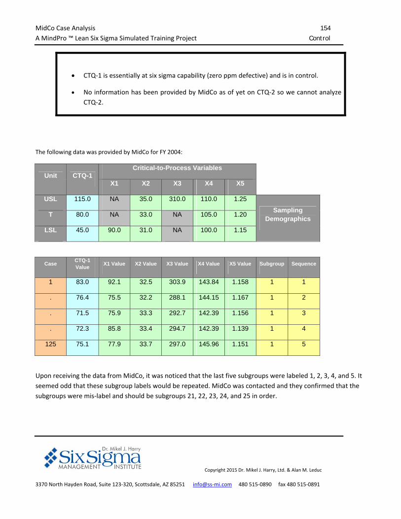
MidCo Case Analysis 154
A MindPro ™ Lean Six Sigma Simulated Training Project Control
Copyright 2015 Dr. Mikel J. Harry, Ltd. & Alan M. Leduc
3370 North Hayden Road, Suite 123‐320, Scottsdale, AZ 85251 info@ss‐mi.com 480 515‐0890 fax 480 515‐0891
CTQ‐1 is essentially at six sigma capability (zero ppm defective) and is in control.
No information has been provided by MidCo as of yet on CTQ‐2 so we cannot analyze
CTQ‐2.
The following data was provided by MidCo for FY 2004:
Unit CTQ-1 Critical-to-Process Variables
X1 X2 X3 X4 X5
USL 115.0 NA 35.0 310.0 110.0 1.25
Sampling Demographics
T 80.0 NA 33.0 NA 105.0 1.20
LSL 45.0 90.0 31.0 NA 100.0 1.15
Case CTQ-1 Value
X1 Value X2 Value X3 Value X4 Value X5 Value Subgroup Sequence
1 83.0 92.1 32.5 303.9 143.84 1.158 1 1
. 76.4 75.5 32.2 288.1 144.15 1.167 1 2
. 71.5 75.9 33.3 292.7 142.39 1.156 1 3
. 72.3 85.8 33.4 294.7 142.39 1.139 1 4
125 75.1 77.9 33.7 297.0 145.96 1.151 1 5
Upon receiving the data from MidCo, it was noticed that the last five subgroups were labeled 1, 2, 3, 4, and 5. It
seemed odd that these subgroup labels would be repeated. MidCo was contacted and they confirmed that the
subgroups were mis‐label and should be subgroups 21, 22, 23, 24, and 25 in order.
MidCo Case Analysis 155
A MindPro ™ Lean Six Sigma Simulated Training Project Control
Copyright 2015 Dr. Mikel J. Harry, Ltd. & Alan M. Leduc
3370 North Hayden Road, Suite 123‐320, Scottsdale, AZ 85251 info@ss‐mi.com 480 515‐0890 fax 480 515‐0891
Analysis for Control
One of the first steps in the control phase is to analyze the data to ensure that it is in statistical control. Note: No
information has been provided by MidCo as of yet on CTQ‐2 so we cannot analyze CTQ‐2 and the variables as
they relate to CTQ‐2.
Variable X‐bar / S Charts Comments
CTQ‐1
Value
252321191715131197531
85
80
75
70
Sample
Sa
mp
le M
ea
n
__X=77.22
UC L=84.86
LC L=69.58
252321191715131197531
10.0
7.5
5.0
2.5
0.0
Sample
Sa
mp
le S
tDe
v
_S=5.35
UC L=11.18
LC L=0
Xbar-S Chart of CTQ-1 Value
In statistical control. No apparent
assignable causes.
X1
Value
252321191715131197531
90
85
80
75
70
Sample
Sa
mp
le M
ea
n
__X=80.39
UC L=89.10
LC L=71.68
252321191715131197531
12
9
6
3
0
Sample
Sa
mp
le S
tDe
v
_S=6.10
UC L=12.75
LC L=0
Xbar-S Chart of X1 Value
In statistical control. No apparent
assignable causes.
Candidate Analysis Required for
Black Belt and Green Belt ‐Industrial
See MidCo Exam Workbook:
Control Task 1
Control Task 2
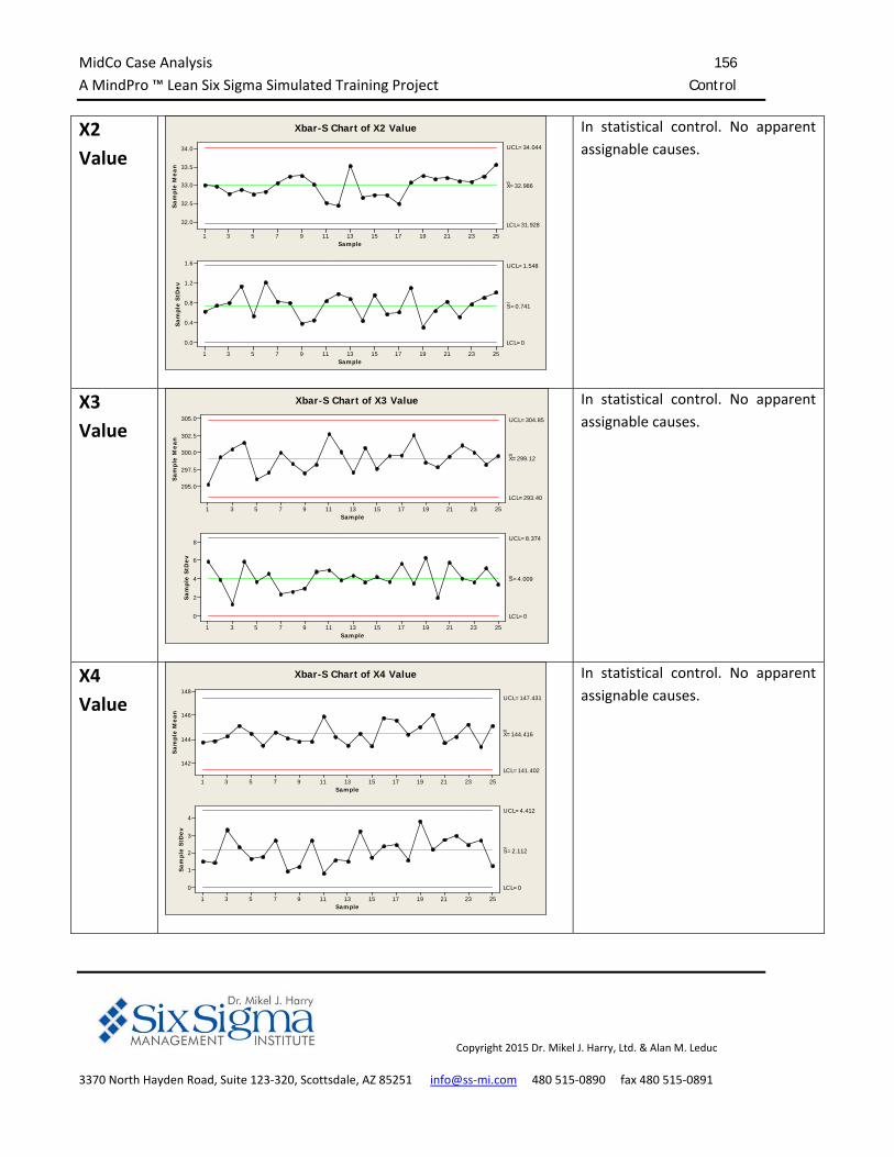
MidCo Case Analysis 156
A MindPro ™ Lean Six Sigma Simulated Training Project Control
Copyright 2015 Dr. Mikel J. Harry, Ltd. & Alan M. Leduc
3370 North Hayden Road, Suite 123‐320, Scottsdale, AZ 85251 info@ss‐mi.com 480 515‐0890 fax 480 515‐0891
X2
Value
252321191715131197531
34.0
33.5
33.0
32.5
32.0
Sample
Sa
mp
le M
ea
n__X=32.986
UC L=34.044
LC L=31.928
252321191715131197531
1.6
1.2
0.8
0.4
0.0
Sample
Sa
mp
le S
tDe
v
_S=0.741
UC L=1.548
LC L=0
Xbar-S Chart of X2 Value
In statistical control. No apparent
assignable causes.
X3
Value
252321191715131197531
305.0
302.5
300.0
297.5
295.0
Sample
Sa
mp
le M
ea
n
__X=299.12
UC L=304.85
LC L=293.40
252321191715131197531
8
6
4
2
0
Sample
Sa
mp
le S
tDe
v
_S=4.009
UC L=8.374
LC L=0
Xbar-S Chart of X3 Value
In statistical control. No apparent
assignable causes.
X4
Value
252321191715131197531
148
146
144
142
Sample
Sa
mp
le M
ea
n
__X=144.416
UC L=147.431
LC L=141.402
252321191715131197531
4
3
2
1
0
Sample
Sa
mp
le S
tDe
v
_S=2.112
UC L=4.412
LC L=0
Xbar-S Chart of X4 Value
In statistical control. No apparent
assignable causes.
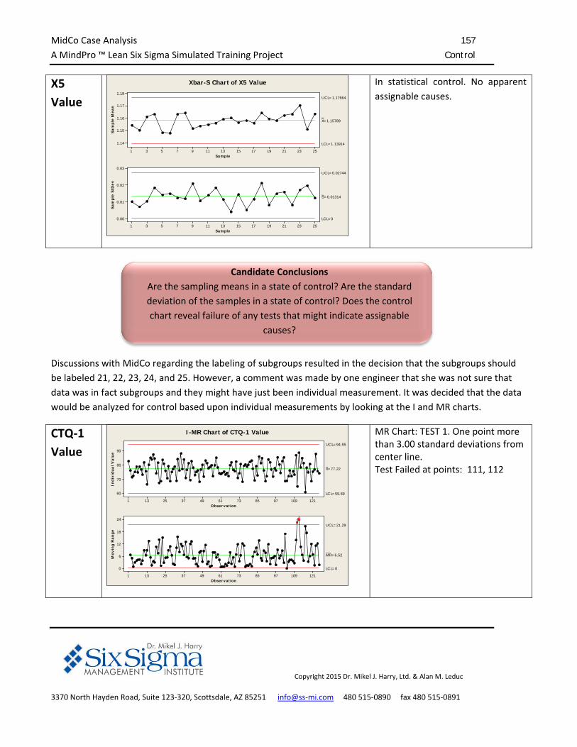
MidCo Case Analysis 157
A MindPro ™ Lean Six Sigma Simulated Training Project Control
Copyright 2015 Dr. Mikel J. Harry, Ltd. & Alan M. Leduc
3370 North Hayden Road, Suite 123‐320, Scottsdale, AZ 85251 info@ss‐mi.com 480 515‐0890 fax 480 515‐0891
X5
Value
252321191715131197531
1.18
1.17
1.16
1.15
1.14
Sample
Sa
mp
le M
ea
n__X=1.15789
UC L=1.17664
LC L=1.13914
252321191715131197531
0.03
0.02
0.01
0.00
Sample
Sa
mp
le S
tDe
v
_S=0.01314
UC L=0.02744
LC L=0
Xbar-S Chart of X5 Value
In statistical control. No apparent
assignable causes.
Discussions with MidCo regarding the labeling of subgroups resulted in the decision that the subgroups should
be labeled 21, 22, 23, 24, and 25. However, a comment was made by one engineer that she was not sure that
data was in fact subgroups and they might have just been individual measurement. It was decided that the data
would be analyzed for control based upon individual measurements by looking at the I and MR charts.
CTQ‐1
Value
12110997857361493725131
90
80
70
60
Observation
Ind
ivid
ua
l V
alu
e
_X=77.22
UC L=94.55
LC L=59.89
12110997857361493725131
24
18
12
6
0
Observation
Mo
vin
g R
an
ge
__MR=6.52
UC L=21.29
LC L=0
11
I-MR Chart of CTQ-1 Value
MR Chart: TEST 1. One point more than 3.00 standard deviations from center line. Test Failed at points: 111, 112
Candidate Conclusions
Are the sampling means in a state of control? Are the standard
deviation of the samples in a state of control? Does the control
chart reveal failure of any tests that might indicate assignable
causes?
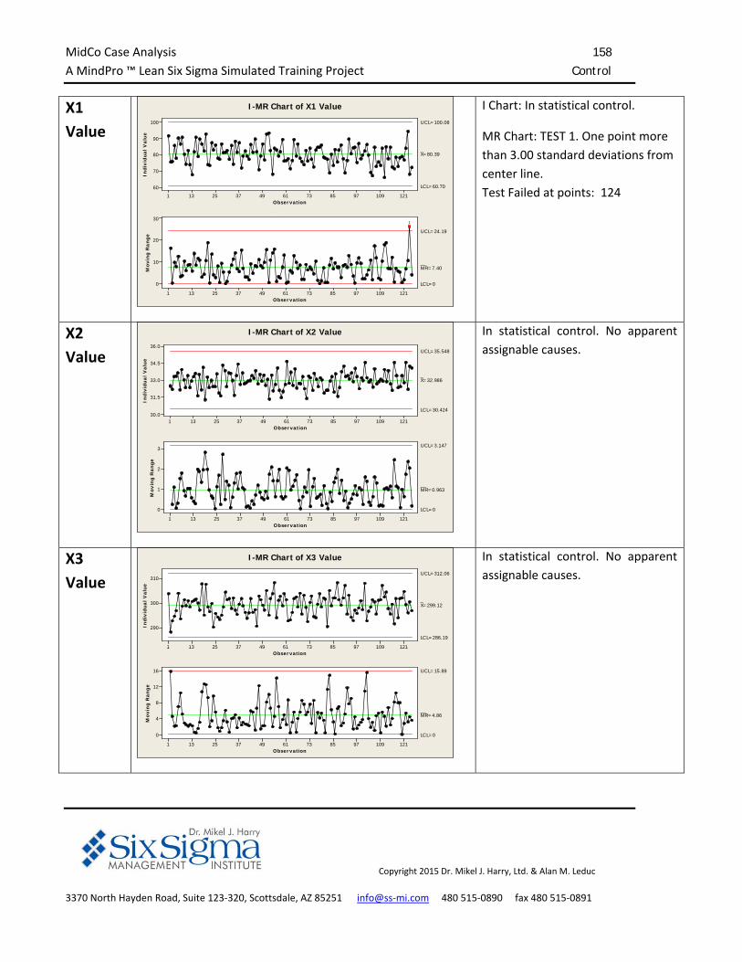
MidCo Case Analysis 158
A MindPro ™ Lean Six Sigma Simulated Training Project Control
Copyright 2015 Dr. Mikel J. Harry, Ltd. & Alan M. Leduc
3370 North Hayden Road, Suite 123‐320, Scottsdale, AZ 85251 info@ss‐mi.com 480 515‐0890 fax 480 515‐0891
X1
Value
12110997857361493725131
100
90
80
70
60
Observation
Ind
ivid
ua
l V
alu
e_X=80.39
UC L=100.08
LC L=60.70
12110997857361493725131
30
20
10
0
Observation
Mo
vin
g R
an
ge
__MR=7.40
UC L=24.19
LC L=0
1
I-MR Chart of X1 Value
I Chart: In statistical control.
MR Chart: TEST 1. One point more
than 3.00 standard deviations from
center line.
Test Failed at points: 124
X2
Value
12110997857361493725131
36.0
34.5
33.0
31.5
30.0
Observation
Ind
ivid
ua
l V
alu
e
_X=32.986
UC L=35.548
LC L=30.424
12110997857361493725131
3
2
1
0
Observation
Mo
vin
g R
an
ge
__MR=0.963
UC L=3.147
LC L=0
I-MR Chart of X2 Value
In statistical control. No apparent
assignable causes.
X3
Value
12110997857361493725131
310
300
290
Observation
Ind
ivid
ua
l V
alu
e
_X=299.12
UC L=312.06
LC L=286.19
12110997857361493725131
16
12
8
4
0
Observation
Mo
vin
g R
an
ge
__MR=4.86
UC L=15.89
LC L=0
I-MR Chart of X3 Value
In statistical control. No apparent
assignable causes.
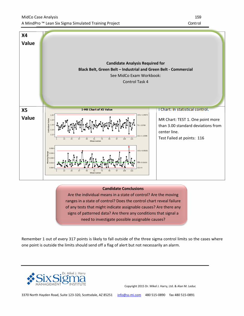
MidCo Case Analysis 159
A MindPro ™ Lean Six Sigma Simulated Training Project Control
Copyright 2015 Dr. Mikel J. Harry, Ltd. & Alan M. Leduc
3370 North Hayden Road, Suite 123‐320, Scottsdale, AZ 85251 info@ss‐mi.com 480 515‐0890 fax 480 515‐0891
X4
Value
12110997857361493725131
152
148
144
140
Observation
Ind
ivid
ua
l V
alu
e_X=144.42
UC L=150.94
LC L=137.89
12110997857361493725131
8
6
4
2
0
Observation
Mo
vin
g R
an
ge
__MR=2.453
UC L=8.014
LC L=0
1
1
I-MR Chart of X4 Value
I Chart: TEST 1. One point more
than 3.00 standard deviations from
center line.
Test Failed at points: 92
MR Chart: TEST 1. One point more
than 3.00 standard deviations from
center line.
Test Failed at points: 16
X5
Value
12110997857361493725131
1.20
1.18
1.16
1.14
1.12
Observation
Ind
ivid
ua
l V
alu
e
_X=1.15789
UC L=1.20072
LC L=1.11506
12110997857361493725131
0.060
0.045
0.030
0.015
0.000
Observation
Mo
vin
g R
an
ge
__MR=0.01610
UC L=0.05261
LC L=0
1
I-MR Chart of X5 Value
I Chart: In statistical control.
MR Chart: TEST 1. One point more
than 3.00 standard deviations from
center line.
Test Failed at points: 116
Remember 1 out of every 317 points is likely to fall outside of the three sigma control limits so the cases where
one point is outside the limits should send off a flag of alert but not necessarily an alarm.
Candidate Analysis Required for
Black Belt, Green Belt – Industrial and Green Belt ‐ Commercial
See MidCo Exam Workbook:
Control Task 4
Candidate Conclusions
Are the individual means in a state of control? Are the moving
ranges in a state of control? Does the control chart reveal failure
of any tests that might indicate assignable causes? Are there any
signs of patterned data? Are there any conditions that signal a
need to investigate possible assignable causes?
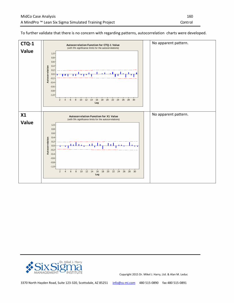
MidCo Case Analysis 160
A MindPro ™ Lean Six Sigma Simulated Training Project Control
Copyright 2015 Dr. Mikel J. Harry, Ltd. & Alan M. Leduc
3370 North Hayden Road, Suite 123‐320, Scottsdale, AZ 85251 info@ss‐mi.com 480 515‐0890 fax 480 515‐0891
To further validate that there is no concern with regarding patterns, autocorrelation charts were developed.
CTQ‐1
Value
30282624222018161412108642
1.0
0.8
0.6
0.4
0.2
0.0
-0.2
-0.4
-0.6
-0.8
-1.0
Lag
Aut
ocor
rela
tion
Autocorrelation Function for CTQ-1 Value(with 5% significance limits for the autocorrelations)
No apparent pattern.
X1
Value
30282624222018161412108642
1.0
0.8
0.6
0.4
0.2
0.0
-0.2
-0.4
-0.6
-0.8
-1.0
Lag
Aut
ocor
rela
tion
Autocorrelation Function for X1 Value(with 5% significance limits for the autocorrelations)
No apparent pattern.
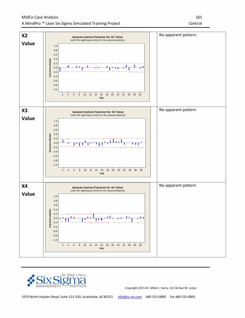
MidCo Case Analysis 161
A MindPro ™ Lean Six Sigma Simulated Training Project Control
Copyright 2015 Dr. Mikel J. Harry, Ltd. & Alan M. Leduc
3370 North Hayden Road, Suite 123‐320, Scottsdale, AZ 85251 info@ss‐mi.com 480 515‐0890 fax 480 515‐0891
X2
Value
30282624222018161412108642
1.0
0.8
0.6
0.4
0.2
0.0
-0.2
-0.4
-0.6
-0.8
-1.0
Lag
Aut
ocor
rela
tion
Autocorrelation Function for X2 Value(with 5% significance limits for the autocorrelations)
No apparent pattern.
X3
Value
30282624222018161412108642
1.0
0.8
0.6
0.4
0.2
0.0
-0.2
-0.4
-0.6
-0.8
-1.0
Lag
Aut
ocor
rela
tion
Autocorrelation Function for X3 Value(with 5% significance limits for the autocorrelations)
No apparent pattern
X4
Value
30282624222018161412108642
1.0
0.8
0.6
0.4
0.2
0.0
-0.2
-0.4
-0.6
-0.8
-1.0
Lag
Aut
ocor
rela
tion
Autocorrelation Function for X4 Value(with 5% significance limits for the autocorrelations)
No apparent pattern
MidCo Case Analysis 162
A MindPro ™ Lean Six Sigma Simulated Training Project Control
Copyright 2015 Dr. Mikel J. Harry, Ltd. & Alan M. Leduc
3370 North Hayden Road, Suite 123‐320, Scottsdale, AZ 85251 info@ss‐mi.com 480 515‐0890 fax 480 515‐0891
X5
Value
30282624222018161412108642
1.0
0.8
0.6
0.4
0.2
0.0
-0.2
-0.4
-0.6
-0.8
-1.0
Lag
Aut
ocor
rela
tion
Autocorrelation Function for X5 Value(with 5% significance limits for the autocorrelations)
No apparent pattern
Candidate Analysis Required for
Black Belt and Green Belt ‐Industrial
See MidCo Exam Workbook:
Control Task 5
Candidate Conclusions
Are there any lags that are beyond the statistical control limits?
Is there any indication that there is a patterned behavior over
time?
MidCo Case Analysis 163
A MindPro ™ Lean Six Sigma Simulated Training Project Control
Copyright 2015 Dr. Mikel J. Harry, Ltd. & Alan M. Leduc
3370 North Hayden Road, Suite 123‐320, Scottsdale, AZ 85251 info@ss‐mi.com 480 515‐0890 fax 480 515‐0891
Analysis of Capability
Having analyzed the data for control, the data was then analyzed for capability.
CTQ‐1
1101009080706050
LSL USL
LSL 45Target *USL 115Sample Mean 77.2192Sample N 125StDev (Within) 5.69228StDev (O v erall) 5.57867
Process Data
Z.Bench 5.66Z.LSL 5.66Z.USL 6.64C pk 1.89
Z.Bench 5.78Z.LSL 5.78Z.USL 6.77Ppk 1.93C pm *
O v erall C apability
Potential (Within) C apability
PPM < LSL 0.00PPM > USL 0.00PPM Total 0.00
O bserv ed PerformancePPM < LSL 0.01PPM > USL 0.00PPM Total 0.01
Exp. Within PerformancePPM < LSL 0.00PPM > USL 0.00PPM Total 0.00
Exp. O v erall Performance
WithinOverall
Process Capability of CTQ-1 Value
As a reminder Z.Bench is equal to Cp*3. Since we have elected to show Z.Bench values instead of Cp values, we
can calculate Cp by dividing Z.Bench by 3.
Candidate Analysis Required for
Black Belt and Green Belt ‐ Industrial
See MidCo Exam Workbook:
Control Task 3
Candidate Conclusions
What is the sustainable (overall) capability? What index provides
this information? What is the instantaneous (potential
capability? What index provides this information? What is the Z‐
Bench capability?
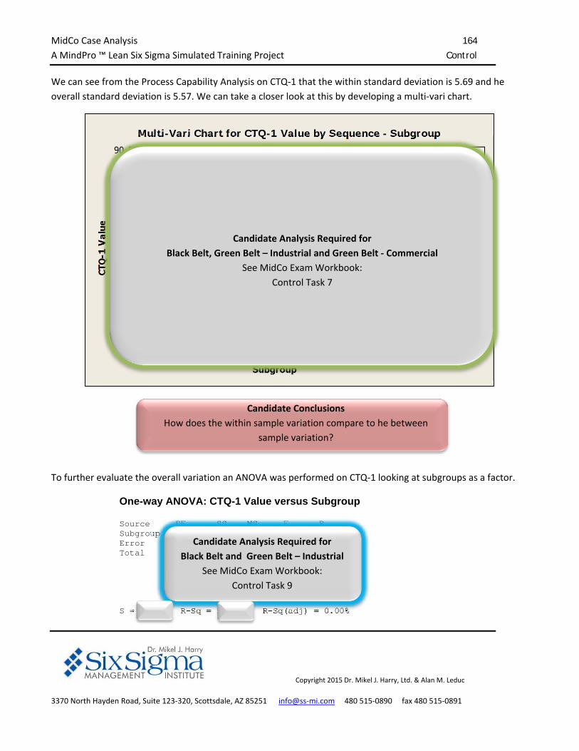
MidCo Case Analysis 164
A MindPro ™ Lean Six Sigma Simulated Training Project Control
Copyright 2015 Dr. Mikel J. Harry, Ltd. & Alan M. Leduc
3370 North Hayden Road, Suite 123‐320, Scottsdale, AZ 85251 info@ss‐mi.com 480 515‐0890 fax 480 515‐0891
We can see from the Process Capability Analysis on CTQ‐1 that the within standard deviation is 5.69 and he
overall standard deviation is 5.57. We can take a closer look at this by developing a multi‐vari chart.
2019181716151413121110 9 8 7 6 5 4 3 2 1
90
85
80
75
70
Subgroup
CTQ
-1 V
alue
12345
Sequence
Multi-Vari Chart for CTQ-1 Value by Sequence - Subgroup
To further evaluate the overall variation an ANOVA was performed on CTQ‐1 looking at subgroups as a factor.
One-way ANOVA: CTQ-1 Value versus Subgroup Source DF SS MS F P Subgroup 24 635.0 26.5 0.82 0.703 Error 100 3224.0 32.2 Total 124 3859.1 S = 5.678 R-Sq = 16.46% R-Sq(adj) = 0.00%
Candidate Analysis Required for
Black Belt, Green Belt – Industrial and Green Belt ‐ Commercial
See MidCo Exam Workbook:
Control Task 7
Candidate Conclusions
How does the within sample variation compare to he between
sample variation?
Candidate Analysis Required for
Black Belt and Green Belt – Industrial
See MidCo Exam Workbook:
Control Task 9
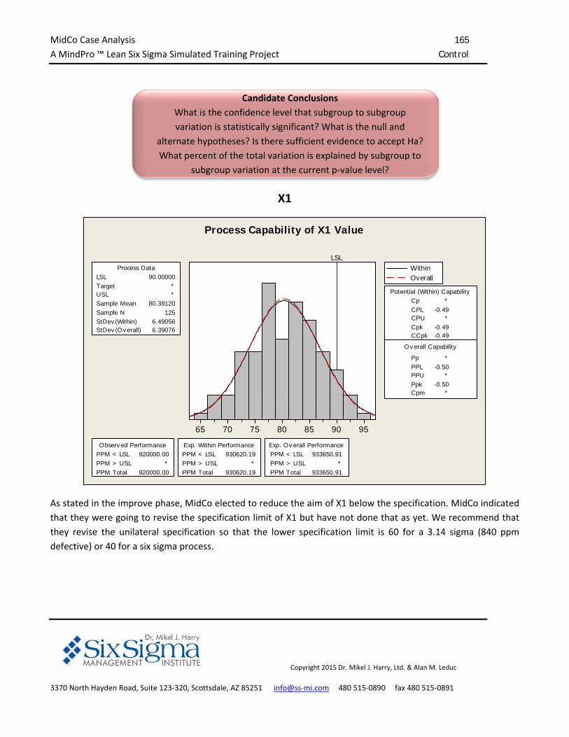
MidCo Case Analysis 165
A MindPro ™ Lean Six Sigma Simulated Training Project Control
Copyright 2015 Dr. Mikel J. Harry, Ltd. & Alan M. Leduc
3370 North Hayden Road, Suite 123‐320, Scottsdale, AZ 85251 info@ss‐mi.com 480 515‐0890 fax 480 515‐0891
X1
95908580757065
LSLProcess Data
Sample N 125StDev (Within) 6.49056StDev (O v erall) 6.39076
LSL 90.00000Target *USL *Sample Mean 80.39120
Potential (Within) C apability
C C pk -0.49
O v erall C apability
Pp *PPL -0.50PPU *Ppk
C p
-0.50C pm *
*C PL -0.49C PU *C pk -0.49
O bserv ed PerformancePPM < LSL 920000.00PPM > USL *PPM Total 920000.00
Exp. Within PerformancePPM < LSL 930620.19PPM > USL *PPM Total 930620.19
Exp. O v erall PerformancePPM < LSL 933650.91PPM > USL *PPM Total 933650.91
WithinOverall
Process Capability of X1 Value
As stated in the improve phase, MidCo elected to reduce the aim of X1 below the specification. MidCo indicated
that they were going to revise the specification limit of X1 but have not done that as yet. We recommend that
they revise the unilateral specification so that the lower specification limit is 60 for a 3.14 sigma (840 ppm
defective) or 40 for a six sigma process.
Candidate Conclusions
What is the confidence level that subgroup to subgroup
variation is statistically significant? What is the null and
alternate hypotheses? Is there sufficient evidence to accept Ha?
What percent of the total variation is explained by subgroup to
subgroup variation at the current p‐value level?
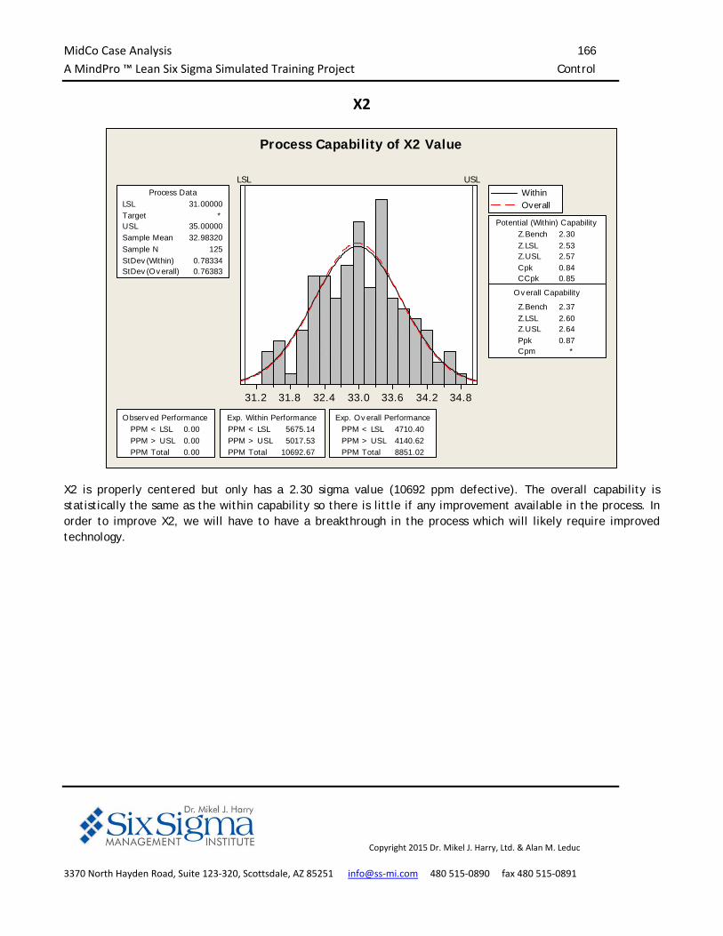
MidCo Case Analysis 166
A MindPro ™ Lean Six Sigma Simulated Training Project Control
Copyright 2015 Dr. Mikel J. Harry, Ltd. & Alan M. Leduc
3370 North Hayden Road, Suite 123‐320, Scottsdale, AZ 85251 info@ss‐mi.com 480 515‐0890 fax 480 515‐0891
X2
34.834.233.633.032.431.831.2
LSL USLProcess Data
Sample N 125StDev (Within) 0.78334StDev (O v erall) 0.76383
LSL 31.00000Target *USL 35.00000Sample Mean 32.98320
Potential (Within) C apability
C C pk 0.85
O v erall C apability
Z.Bench 2.37Z.LSL 2.60Z.USL 2.64Ppk
Z.Bench
0.87C pm *
2.30Z.LSL 2.53Z.USL 2.57C pk 0.84
O bserv ed PerformancePPM < LSL 0.00PPM > USL 0.00PPM Total 0.00
Exp. Within PerformancePPM < LSL 5675.14PPM > USL 5017.53PPM Total 10692.67
Exp. O v erall PerformancePPM < LSL 4710.40PPM > USL 4140.62PPM Total 8851.02
WithinOverall
Process Capability of X2 Value
X2 is properly centered but only has a 2.30 sigma value (10692 ppm defective). The overall capability is statistically the same as the within capability so there is little if any improvement available in the process. In order to improve X2, we will have to have a breakthrough in the process which will likely require improved technology.
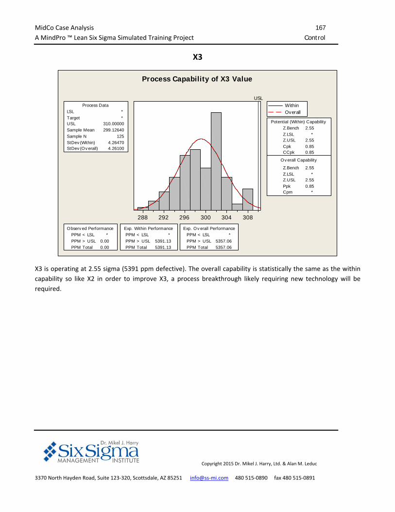
MidCo Case Analysis 167
A MindPro ™ Lean Six Sigma Simulated Training Project Control
Copyright 2015 Dr. Mikel J. Harry, Ltd. & Alan M. Leduc
3370 North Hayden Road, Suite 123‐320, Scottsdale, AZ 85251 info@ss‐mi.com 480 515‐0890 fax 480 515‐0891
X3
308304300296292288
USLProcess Data
Sample N 125StDev (Within) 4.26470StDev (O v erall) 4.26100
LSL *Target *USL 310.00000Sample Mean 299.12640
Potential (Within) C apability
C C pk 0.85
O v erall C apability
Z.Bench 2.55Z.LSL *Z.USL 2.55Ppk
Z.Bench
0.85C pm *
2.55Z.LSL *Z.USL 2.55C pk 0.85
O bserv ed PerformancePPM < LSL *PPM > USL 0.00PPM Total 0.00
Exp. Within PerformancePPM < LSL *PPM > USL 5391.13PPM Total 5391.13
Exp. O v erall PerformancePPM < LSL *PPM > USL 5357.06PPM Total 5357.06
WithinOverall
Process Capability of X3 Value
X3 is operating at 2.55 sigma (5391 ppm defective). The overall capability is statistically the same as the within
capability so like X2 in order to improve X3, a process breakthrough likely requiring new technology will be
required.
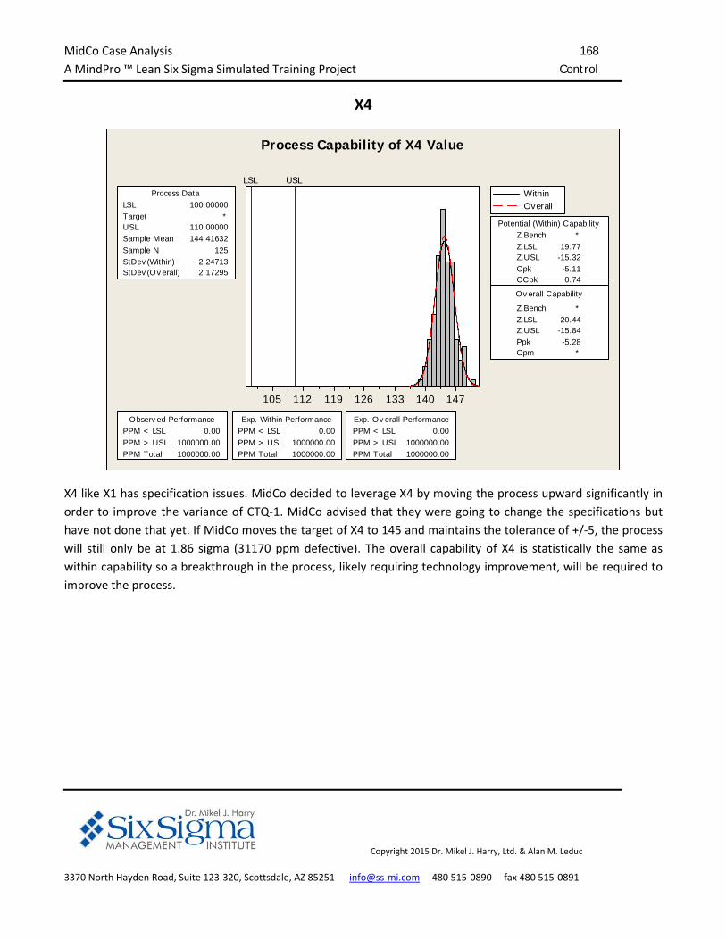
MidCo Case Analysis 168
A MindPro ™ Lean Six Sigma Simulated Training Project Control
Copyright 2015 Dr. Mikel J. Harry, Ltd. & Alan M. Leduc
3370 North Hayden Road, Suite 123‐320, Scottsdale, AZ 85251 info@ss‐mi.com 480 515‐0890 fax 480 515‐0891
X4
147140133126119112105
LSL USLProcess Data
Sample N 125StDev (Within) 2.24713StDev (O v erall) 2.17295
LSL 100.00000Target *USL 110.00000Sample Mean 144.41632
Potential (Within) C apability
C C pk 0.74
O v erall C apability
Z.Bench *Z.LSL 20.44Z.USL -15.84Ppk
Z.Bench
-5.28C pm *
*Z.LSL 19.77Z.USL -15.32C pk -5.11
O bserv ed PerformancePPM < LSL 0.00PPM > USL 1000000.00PPM Total 1000000.00
Exp. Within PerformancePPM < LSL 0.00PPM > USL 1000000.00PPM Total 1000000.00
Exp. O v erall PerformancePPM < LSL 0.00PPM > USL 1000000.00PPM Total 1000000.00
WithinOverall
Process Capability of X4 Value
X4 like X1 has specification issues. MidCo decided to leverage X4 by moving the process upward significantly in
order to improve the variance of CTQ‐1. MidCo advised that they were going to change the specifications but
have not done that yet. If MidCo moves the target of X4 to 145 and maintains the tolerance of +/‐5, the process
will still only be at 1.86 sigma (31170 ppm defective). The overall capability of X4 is statistically the same as
within capability so a breakthrough in the process, likely requiring technology improvement, will be required to
improve the process.
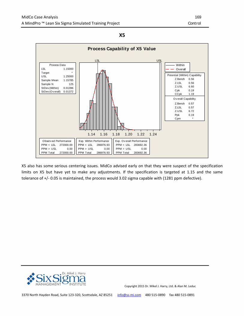
MidCo Case Analysis 169
A MindPro ™ Lean Six Sigma Simulated Training Project Control
Copyright 2015 Dr. Mikel J. Harry, Ltd. & Alan M. Leduc
3370 North Hayden Road, Suite 123‐320, Scottsdale, AZ 85251 info@ss‐mi.com 480 515‐0890 fax 480 515‐0891
X5
1.241.221.201.181.161.14
LSL USLProcess Data
Sample N 125StDev (Within) 0.01396StDev (O v erall) 0.01372
LSL 1.15000Target *USL 1.25000Sample Mean 1.15785
Potential (Within) C apability
C C pk 1.19
O v erall C apability
Z.Bench 0.57Z.LSL 0.57Z.USL 6.72Ppk
Z.Bench
0.19C pm *
0.56Z.LSL 0.56Z.USL 6.60C pk 0.19
O bserv ed PerformancePPM < LSL 272000.00PPM > USL 0.00PPM Total 272000.00
Exp. Within PerformancePPM < LSL 286976.93PPM > USL 0.00PPM Total 286976.93
Exp. O v erall PerformancePPM < LSL 283692.36PPM > USL 0.00PPM Total 283692.36
WithinOverall
Process Capability of X5 Value
X5 also has some serious centering issues. MidCo advised early on that they were suspect of the specification
limits on X5 but have yet to make any adjustments. If the specification is targeted at 1.15 and the same
tolerance of +/‐ 0.05 is maintained, the process would 3.02 sigma capable with (1281 ppm defective).
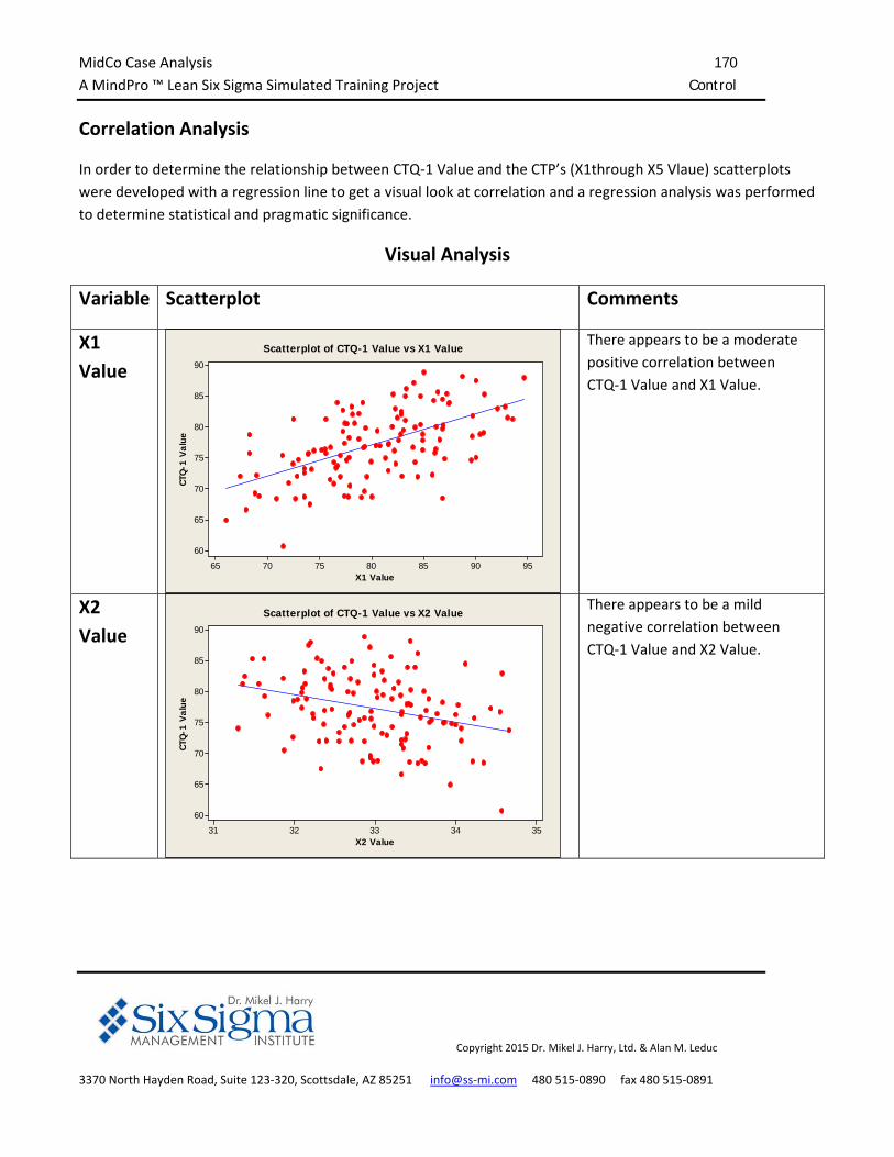
MidCo Case Analysis 170
A MindPro ™ Lean Six Sigma Simulated Training Project Control
Copyright 2015 Dr. Mikel J. Harry, Ltd. & Alan M. Leduc
3370 North Hayden Road, Suite 123‐320, Scottsdale, AZ 85251 info@ss‐mi.com 480 515‐0890 fax 480 515‐0891
Correlation Analysis
In order to determine the relationship between CTQ‐1 Value and the CTP’s (X1through X5 Vlaue) scatterplots
were developed with a regression line to get a visual look at correlation and a regression analysis was performed
to determine statistical and pragmatic significance.
Visual Analysis
Variable Scatterplot Comments
X1
Value
95908580757065
90
85
80
75
70
65
60
X1 Value
CTQ
-1 V
alue
Scatterplot of CTQ-1 Value vs X1 ValueThere appears to be a moderate
positive correlation between
CTQ‐1 Value and X1 Value.
X2
Value
3534333231
90
85
80
75
70
65
60
X2 Value
CTQ
-1 V
alue
Scatterplot of CTQ-1 Value vs X2 Value
There appears to be a mild
negative correlation between
CTQ‐1 Value and X2 Value.
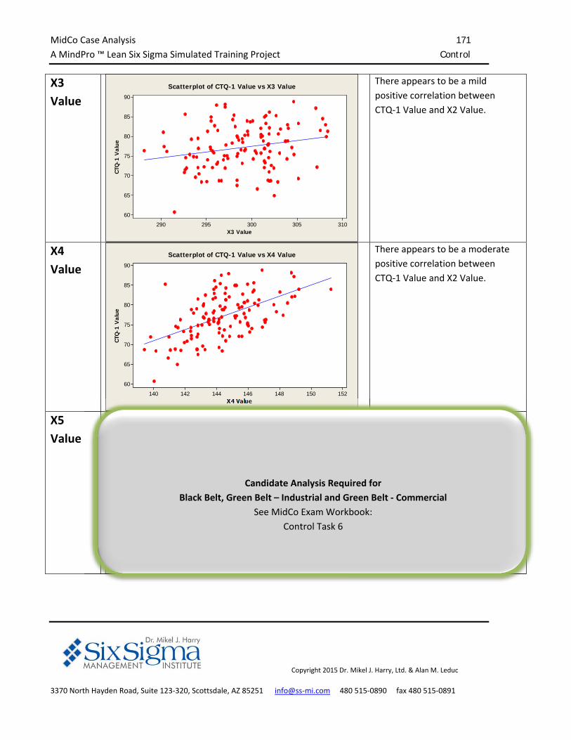
MidCo Case Analysis 171
A MindPro ™ Lean Six Sigma Simulated Training Project Control
Copyright 2015 Dr. Mikel J. Harry, Ltd. & Alan M. Leduc
3370 North Hayden Road, Suite 123‐320, Scottsdale, AZ 85251 info@ss‐mi.com 480 515‐0890 fax 480 515‐0891
X3
Value
310305300295290
90
85
80
75
70
65
60
X3 Value
CTQ
-1 V
alue
Scatterplot of CTQ-1 Value vs X3 Value
There appears to be a mild
positive correlation between
CTQ‐1 Value and X2 Value.
X4
Value
152150148146144142140
90
85
80
75
70
65
60
X4 Value
CTQ
-1 V
alue
Scatterplot of CTQ-1 Value vs X4 Value
There appears to be a moderate
positive correlation between
CTQ‐1 Value and X2 Value.
X5
Value
1.201.191.181.171.161.151.141.131.12
90
85
80
75
70
65
60
X5 Value
CTQ
-1 V
alue
Scatterplot of CTQ-1 Value vs X5 Value
There appears to be a moderate
positive correlation between
CTQ‐1 Value and X5 Value.
Candidate Analysis Required for
Black Belt, Green Belt – Industrial and Green Belt ‐ Commercial
See MidCo Exam Workbook:
Control Task 6
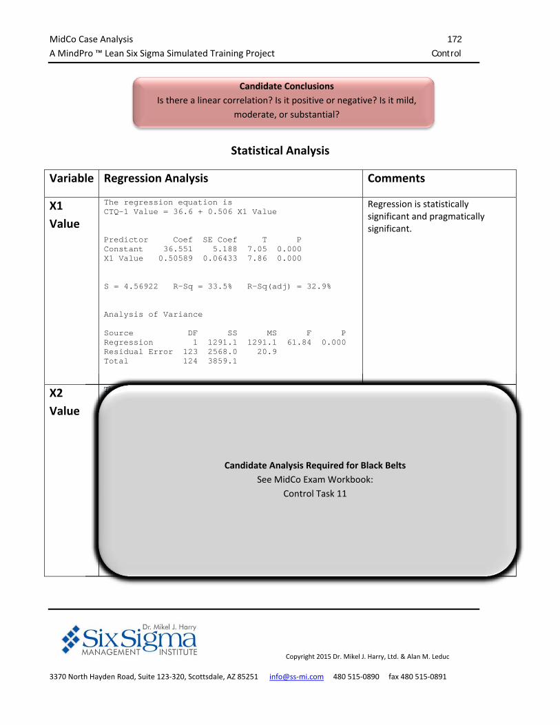
MidCo Case Analysis 172
A MindPro ™ Lean Six Sigma Simulated Training Project Control
Copyright 2015 Dr. Mikel J. Harry, Ltd. & Alan M. Leduc
3370 North Hayden Road, Suite 123‐320, Scottsdale, AZ 85251 info@ss‐mi.com 480 515‐0890 fax 480 515‐0891
Statistical Analysis
Variable Regression Analysis Comments
X1
Value
The regression equation is CTQ-1 Value = 36.6 + 0.506 X1 Value Predictor Coef SE Coef T P Constant 36.551 5.188 7.05 0.000 X1 Value 0.50589 0.06433 7.86 0.000 S = 4.56922 R-Sq = 33.5% R-Sq(adj) = 32.9% Analysis of Variance Source DF SS MS F P Regression 1 1291.1 1291.1 61.84 0.000 Residual Error 123 2568.0 20.9 Total 124 3859.1
Regression is statistically significant and pragmatically significant.
X2
Value
The regression equation is CTQ-1 Value = 151 - 2.23 X2 Value Predictor Coef SE Coef T P Constant 150.65 20.63 7.30 0.000 X2 Value -2.2261 0.6253 -3.56 0.001 S = 5.33327 R-Sq = 9.3% R-Sq(adj) = 8.6% Analysis of Variance Source DF SS MS F P Regression 1 360.48 360.48 12.67 0.001 Residual Error 123 3498.59 28.44 Total 124 3859.07
Regression is statistically
significant but pragmatically
insignificant.
Candidate Conclusions
Is there a linear correlation? Is it positive or negative? Is it mild,
moderate, or substantial?
Candidate Analysis Required for Black Belts
See MidCo Exam Workbook:
Control Task 11
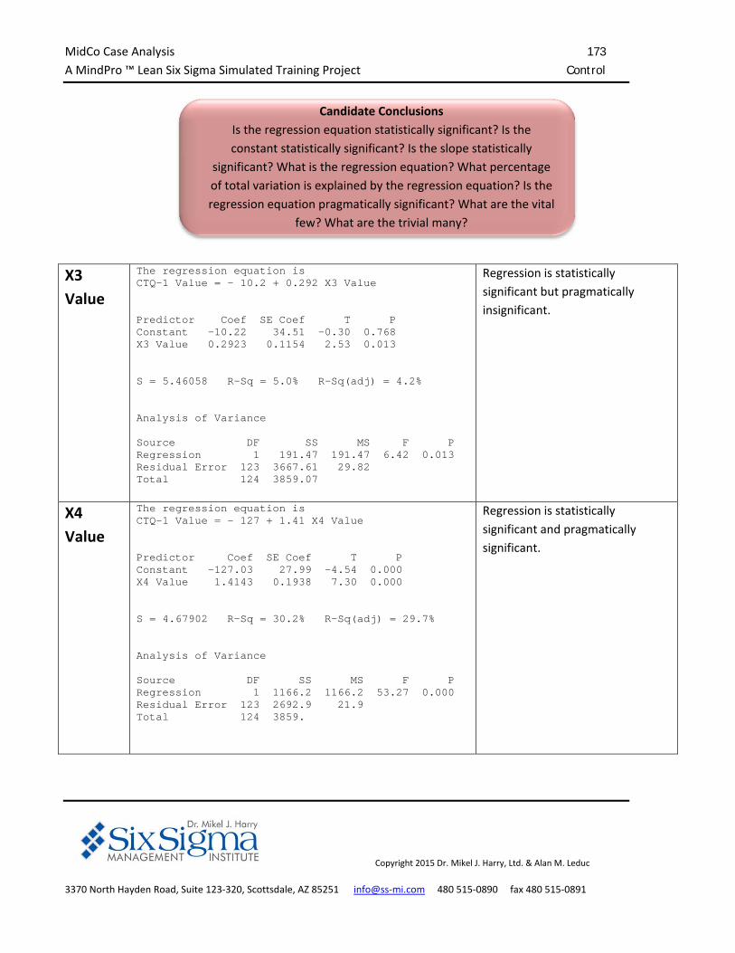
MidCo Case Analysis 173
A MindPro ™ Lean Six Sigma Simulated Training Project Control
Copyright 2015 Dr. Mikel J. Harry, Ltd. & Alan M. Leduc
3370 North Hayden Road, Suite 123‐320, Scottsdale, AZ 85251 info@ss‐mi.com 480 515‐0890 fax 480 515‐0891
X3
Value
The regression equation is CTQ-1 Value = - 10.2 + 0.292 X3 Value Predictor Coef SE Coef T P Constant -10.22 34.51 -0.30 0.768 X3 Value 0.2923 0.1154 2.53 0.013 S = 5.46058 R-Sq = 5.0% R-Sq(adj) = 4.2% Analysis of Variance Source DF SS MS F P Regression 1 191.47 191.47 6.42 0.013 Residual Error 123 3667.61 29.82 Total 124 3859.07
Regression is statistically
significant but pragmatically
insignificant.
X4
Value
The regression equation is CTQ-1 Value = - 127 + 1.41 X4 Value Predictor Coef SE Coef T P Constant -127.03 27.99 -4.54 0.000 X4 Value 1.4143 0.1938 7.30 0.000 S = 4.67902 R-Sq = 30.2% R-Sq(adj) = 29.7% Analysis of Variance Source DF SS MS F P Regression 1 1166.2 1166.2 53.27 0.000 Residual Error 123 2692.9 21.9 Total 124 3859.
Regression is statistically
significant and pragmatically
significant.
Candidate Conclusions
Is the regression equation statistically significant? Is the
constant statistically significant? Is the slope statistically
significant? What is the regression equation? What percentage
of total variation is explained by the regression equation? Is the
regression equation pragmatically significant? What are the vital
few? What are the trivial many?
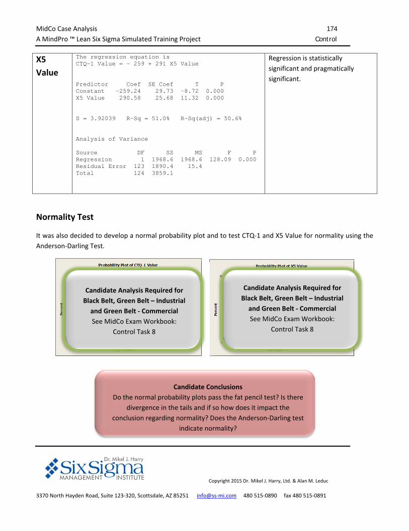
MidCo Case Analysis 174
A MindPro ™ Lean Six Sigma Simulated Training Project Control
Copyright 2015 Dr. Mikel J. Harry, Ltd. & Alan M. Leduc
3370 North Hayden Road, Suite 123‐320, Scottsdale, AZ 85251 info@ss‐mi.com 480 515‐0890 fax 480 515‐0891
X5
Value
The regression equation is CTQ-1 Value = - 259 + 291 X5 Value Predictor Coef SE Coef T P Constant -259.24 29.73 -8.72 0.000 X5 Value 290.58 25.68 11.32 0.000 S = 3.92039 R-Sq = 51.0% R-Sq(adj) = 50.6% Analysis of Variance Source DF SS MS F P Regression 1 1968.6 1968.6 128.09 0.000 Residual Error 123 1890.4 15.4 Total 124 3859.1
Regression is statistically
significant and pragmatically
significant.
Normality Test
It was also decided to develop a normal probability plot and to test CTQ‐1 and X5 Value for normality using the
Anderson‐Darling Test.
9590858075706560
99.9
99
9590
80706050403020
10
5
1
0.1
CTQ-1 Value
Perc
ent
Mean 77.22StDev 5.579N 125AD 0.232P-Value 0.798
Probability Plot of CTQ-1 ValueNormal
1.201.191.181.171.161.151.141.131.121.11
99.9
99
9590
80706050403020
10
5
1
0.1
X5 Value
Perc
ent
Mean 1.158StDev 0.01371N 125AD 0.100P-Value 0.996
Probability Plot of X5 ValueNormal
Candidate Analysis Required for
Black Belt, Green Belt – Industrial
and Green Belt ‐ Commercial
See MidCo Exam Workbook:
Control Task 8
Candidate Analysis Required for
Black Belt, Green Belt – Industrial
and Green Belt ‐ Commercial
See MidCo Exam Workbook:
Control Task 8
Candidate Conclusions
Do the normal probability plots pass the fat pencil test? Is there
divergence in the tails and if so how does it impact the
conclusion regarding normality? Does the Anderson‐Darling test
indicate normality?
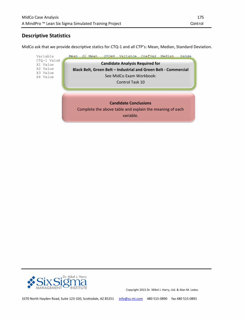
MidCo Case Analysis 175
A MindPro ™ Lean Six Sigma Simulated Training Project Control
Copyright 2015 Dr. Mikel J. Harry, Ltd. & Alan M. Leduc
3370 North Hayden Road, Suite 123‐320, Scottsdale, AZ 85251 info@ss‐mi.com 480 515‐0890 fax 480 515‐0891
Descriptive Statistics
MidCo ask that we provide descriptive statics for CTQ‐1 and all CTP’s: Mean, Median, Standard Deviation.
Variable Mean SE Mean StDev Variance CoefVar Median Range CTQ-1 Value 77.219 0.499 5.579 31.122 7.22 77.000 28.200 X1 Value 80.389 0.571 6.378 40.684 7.93 80.017 28.630 X2 Value 32.986 0.0685 0.766 0.587 2.32 32.984 3.361 X3 Value 299.12 0.380 4.25 18.07 1.42 299.22 20.24 X4 Value 144.42 0.194 2.17 4.70 1.50 144.28 11.88
Candidate Analysis Required for
Black Belt, Green Belt – Industrial and Green Belt ‐ Commercial
See MidCo Exam Workbook:
Control Task 10
Candidate Conclusions
Complete the above table and explain the meaning of each
variable.
MidCo Case Analysis 176
A MindPro ™ Lean Six Sigma Simulated Training Project Control
Copyright 2015 Dr. Mikel J. Harry, Ltd. & Alan M. Leduc
3370 North Hayden Road, Suite 123‐320, Scottsdale, AZ 85251 info@ss‐mi.com 480 515‐0890 fax 480 515‐0891
Moving Average of CTQ‐1 Value
MidCo made a request that we develop a moving average chart for CTQ‐1 Value with a moving average length of
5. The MA chart is a seldom used time weighted control chart.
252321191715131197531
86
84
82
80
78
76
74
72
70
Sample
Mov
ing
Ave
rage
__X=77.22
UCL=80.63
LCL=73.80
Moving Average Chart of CTQ-1 Value
Candidate Analysis Required for
Black Belt, Green Belt – Industrial and Green Belt ‐ Commercial
See MidCo Exam Workbook:
Control Task 12
Candidate Conclusions
Is the moving average of CTQ‐1 in a state of control?
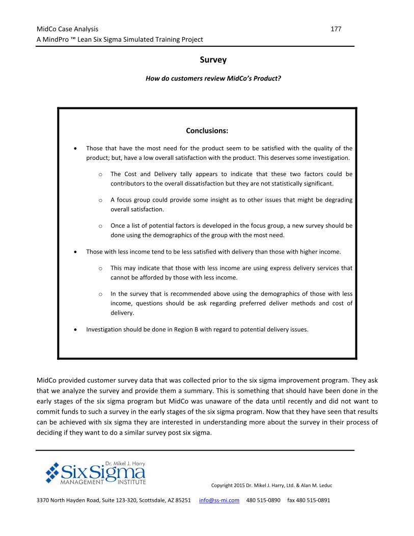
MidCo Case Analysis 177
A MindPro ™ Lean Six Sigma Simulated Training Project
Copyright 2015 Dr. Mikel J. Harry, Ltd. & Alan M. Leduc
3370 North Hayden Road, Suite 123‐320, Scottsdale, AZ 85251 info@ss‐mi.com 480 515‐0890 fax 480 515‐0891
Survey
How do customers review MidCo’s Product?
Conclusions:
Those that have the most need for the product seem to be satisfied with the quality of the
product; but, have a low overall satisfaction with the product. This deserves some investigation.
o The Cost and Delivery tally appears to indicate that these two factors could be
contributors to the overall dissatisfaction but they are not statistically significant.
o A focus group could provide some insight as to other issues that might be degrading
overall satisfaction.
o Once a list of potential factors is developed in the focus group, a new survey should be
done using the demographics of the group with the most need.
Those with less income tend to be less satisfied with delivery than those with higher income.
o This may indicate that those with less income are using express delivery services that
cannot be afforded by those with less income.
o In the survey that is recommended above using the demographics of those with less
income, questions should be ask regarding preferred deliver methods and cost of
delivery.
Investigation should be done in Region B with regard to potential delivery issues.
MidCo provided customer survey data that was collected prior to the six sigma improvement program. They ask
that we analyze the survey and provide them a summary. This is something that should have been done in the
early stages of the six sigma program but MidCo was unaware of the data until recently and did not want to
commit funds to such a survey in the early stages of the six sigma program. Now that they have seen that results
can be achieved with six sigma they are interested in understanding more about the survey in their process of
deciding if they want to do a similar survey post six sigma.
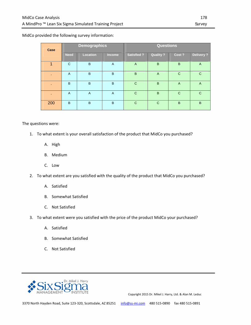
MidCo Case Analysis 178
A MindPro ™ Lean Six Sigma Simulated Training Project Survey
Copyright 2015 Dr. Mikel J. Harry, Ltd. & Alan M. Leduc
3370 North Hayden Road, Suite 123‐320, Scottsdale, AZ 85251 info@ss‐mi.com 480 515‐0890 fax 480 515‐0891
MidCo provided the following survey information:
Case Demographics Questions
Need Location Income Satisfied ? Quality ? Cost ? Delivery ?
1 C B A A B B A
. A B B B A C C
. B B B C B A A
. A A A C B C C
200 B B B C C B B
The questions were:
1. To what extent is your overall satisfaction of the product that MidCo you purchased?
A. High
B. Medium
C. Low
2. To what extent are you satisfied with the quality of the product that MidCo you purchased?
A. Satisfied
B. Somewhat Satisfied
C. Not Satisfied
3. To what extent were you satisfied with the price of the product MidCo your purchased?
A. Satisfied
B. Somewhat Satisfied
C. Not Satisfied
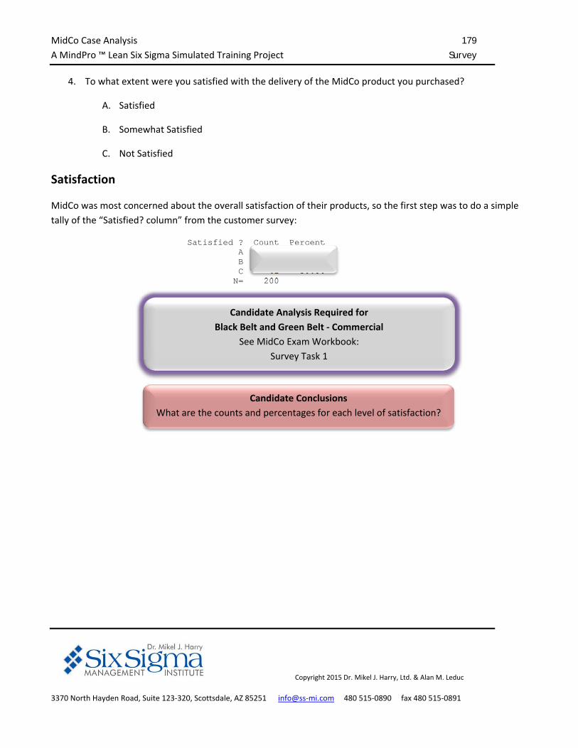
MidCo Case Analysis 179
A MindPro ™ Lean Six Sigma Simulated Training Project Survey
Copyright 2015 Dr. Mikel J. Harry, Ltd. & Alan M. Leduc
3370 North Hayden Road, Suite 123‐320, Scottsdale, AZ 85251 info@ss‐mi.com 480 515‐0890 fax 480 515‐0891
4. To what extent were you satisfied with the delivery of the MidCo product you purchased?
A. Satisfied
B. Somewhat Satisfied
C. Not Satisfied
Satisfaction
MidCo was most concerned about the overall satisfaction of their products, so the first step was to do a simple
tally of the “Satisfied? column” from the customer survey:
Satisfied ? Count Percent A 50 25.00 B 89 44.50 C 61 30.50 N= 200
Candidate Conclusions
What are the counts and percentages for each level of satisfaction?
Candidate Analysis Required for
Black Belt and Green Belt ‐ Commercial
See MidCo Exam Workbook:
Survey Task 1
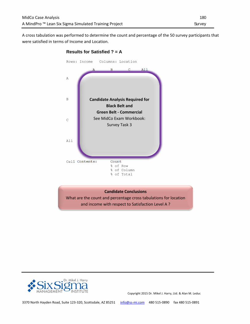
MidCo Case Analysis 180
A MindPro ™ Lean Six Sigma Simulated Training Project Survey
Copyright 2015 Dr. Mikel J. Harry, Ltd. & Alan M. Leduc
3370 North Hayden Road, Suite 123‐320, Scottsdale, AZ 85251 info@ss‐mi.com 480 515‐0890 fax 480 515‐0891
A cross tabulation was performed to determine the count and percentage of the 50 survey participants that
were satisfied in terms of Income and Location.
Results for Satisfied ? = A Rows: Income Columns: Location A B C All A 3 11 4 18 16.67 61.11 22.22 100.00 17.65 50.00 36.36 36.00 6 22 8 36 B 10 10 5 25 40.00 40.00 20.00 100.00 58.82 45.45 45.45 50.00 20 20 10 50 C 4 1 2 7 57.14 14.29 28.57 100.00 23.53 4.55 18.18 14.00 8 2 4 14 All 17 22 11 50 34.00 44.00 22.00 100.00 100.00 100.00 100.00 100.00 34 44 22 100 Cell Contents: Count % of Row % of Column % of Total
Candidate Conclusions
What are the count and percentage cross tabulations for location
and income with respect to Satisfaction Level A ?
Candidate Analysis Required for
Black Belt and
Green Belt ‐ Commercial
See MidCo Exam Workbook:
Survey Task 3
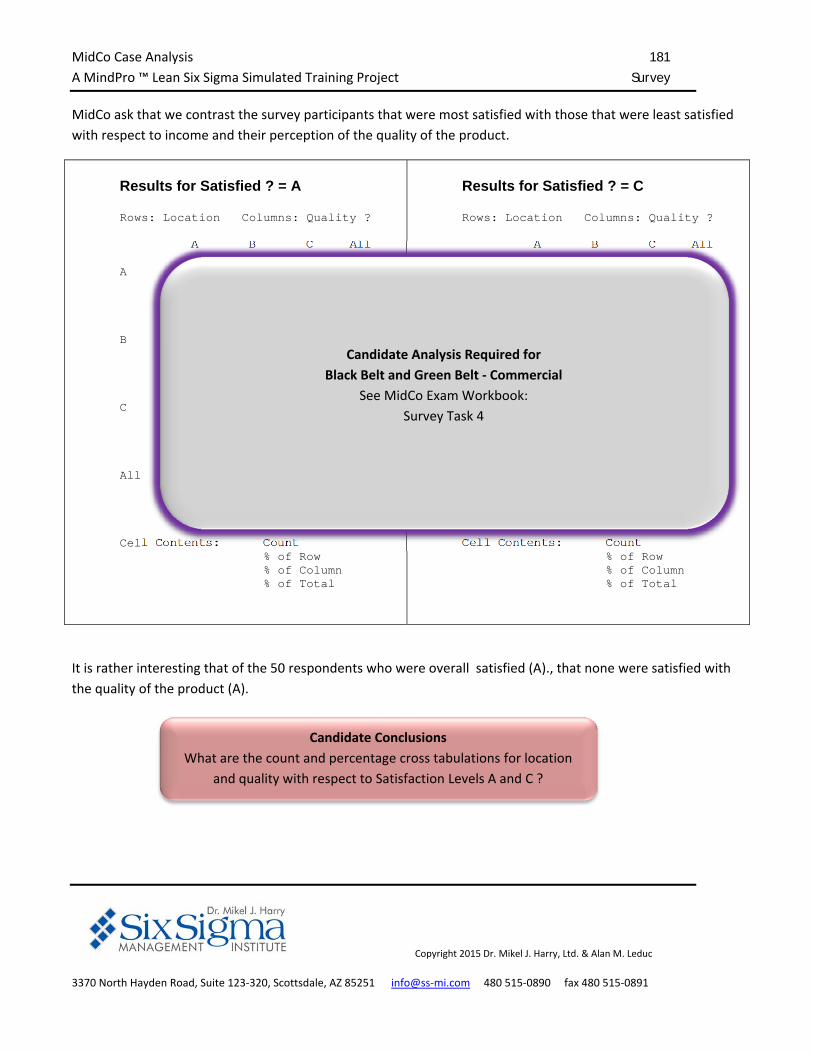
MidCo Case Analysis 181
A MindPro ™ Lean Six Sigma Simulated Training Project Survey
Copyright 2015 Dr. Mikel J. Harry, Ltd. & Alan M. Leduc
3370 North Hayden Road, Suite 123‐320, Scottsdale, AZ 85251 info@ss‐mi.com 480 515‐0890 fax 480 515‐0891
MidCo ask that we contrast the survey participants that were most satisfied with those that were least satisfied
with respect to income and their perception of the quality of the product.
Results for Satisfied ? = A Rows: Location Columns: Quality ? A B C All A 0 7 10 17 0.00 41.18 58.82 100.00 * 33.33 34.48 34.00 0 14 20 34 B 0 10 12 22 0.00 45.45 54.55 100.00 * 47.62 41.38 44.00 0 20 24 44 C 0 4 7 11 0.00 36.36 63.64 100.00 * 19.05 24.14 22.00 0 8 14 22 All 0 21 29 50 0.00 42.00 58.00 100.00 * 100.00 100.00 100.00 0 42 58 100 Cell Contents: Count % of Row % of Column % of Total
Results for Satisfied ? = C Rows: Location Columns: Quality ? A B C All A 0 11 7 18 0.00 61.11 38.89 100.00 * 35.48 23.33 29.51 0.00 18.03 11.48 29.51 B 0 11 13 24 0.00 45.83 54.17 100.00 * 35.48 43.33 39.34 0.00 18.03 21.31 39.34 C 0 9 10 19 0.00 47.37 52.63 100.00 * 29.03 33.33 31.15 0.00 14.75 16.39 31.15 All 0 31 30 61 0.00 50.82 49.18 100.00 * 100.00 100.00 100.00 0.00 50.82 49.18 100.00 Cell Contents: Count % of Row % of Column % of Total
It is rather interesting that of the 50 respondents who were overall satisfied (A)., that none were satisfied with
the quality of the product (A).
Candidate Conclusions
What are the count and percentage cross tabulations for location
and quality with respect to Satisfaction Levels A and C ?
Candidate Analysis Required for
Black Belt and Green Belt ‐ Commercial
See MidCo Exam Workbook:
Survey Task 4
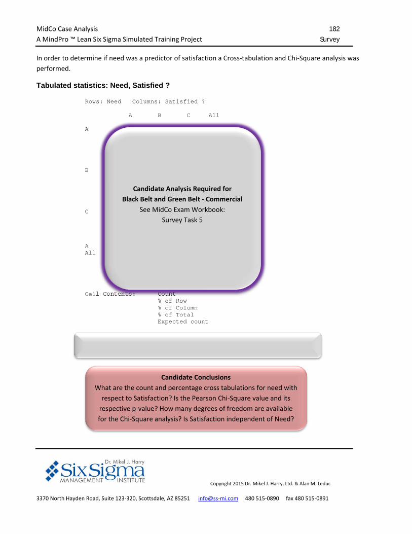
MidCo Case Analysis 182
A MindPro ™ Lean Six Sigma Simulated Training Project Survey
Copyright 2015 Dr. Mikel J. Harry, Ltd. & Alan M. Leduc
3370 North Hayden Road, Suite 123‐320, Scottsdale, AZ 85251 info@ss‐mi.com 480 515‐0890 fax 480 515‐0891
In order to determine if need was a predictor of satisfaction a Cross‐tabulation and Chi‐Square analysis was
performed.
Tabulated statistics: Need, Satisfied ? Rows: Need Columns: Satisfied ? A B C All A 0 39 26 65 0.00 60.00 40.00 100.00 0.00 43.82 42.62 32.50 0.00 19.50 13.00 32.50 16.25 28.93 19.82 65.00 B 0 50 35 85 0.00 58.82 41.18 100.00 0.00 56.18 57.38 42.50 0.00 25.00 17.50 42.50 21.25 37.83 25.93 85.00 C 50 0 0 50 100.00 0.00 0.00 100.00 100.00 0.00 0.00 25.00 25.00 0.00 0.00 25.00 12.50 22.25 15.25 50.00 A All 50 89 61 200 25.00 44.50 30.50 100.00 100.00 100.00 100.00 100.00 25.00 44.50 30.50 100.00 50.00 89.00 61.00 200.00 Cell Contents: Count % of Row % of Column % of Total Expected count Pearson Chi-Square = 200.028, DF = 4, P-Value = 0.000 Likelihood Ratio Chi-Square = 224.955, DF = 4, P-Value = 0.000
Candidate Analysis Required for
Black Belt and Green Belt ‐ Commercial
See MidCo Exam Workbook:
Survey Task 5
Candidate Conclusions
What are the count and percentage cross tabulations for need with
respect to Satisfaction? Is the Pearson Chi‐Square value and its
respective p‐value? How many degrees of freedom are available
for the Chi‐Square analysis? Is Satisfaction independent of Need?
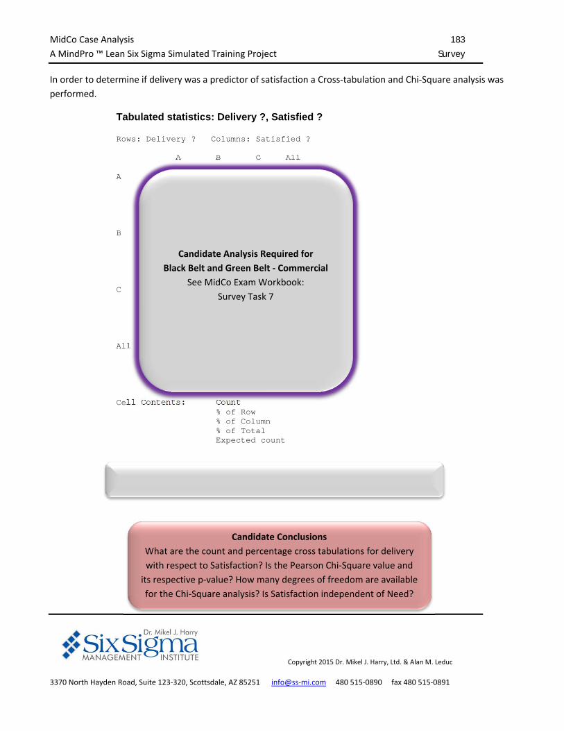
MidCo Case Analysis 183
A MindPro ™ Lean Six Sigma Simulated Training Project Survey
Copyright 2015 Dr. Mikel J. Harry, Ltd. & Alan M. Leduc
3370 North Hayden Road, Suite 123‐320, Scottsdale, AZ 85251 info@ss‐mi.com 480 515‐0890 fax 480 515‐0891
In order to determine if delivery was a predictor of satisfaction a Cross‐tabulation and Chi‐Square analysis was
performed.
Tabulated statistics: Delivery ?, Satisfied ? Rows: Delivery ? Columns: Satisfied ? A B C All A 17 31 19 67 25.37 46.27 28.36 100.00 34.00 34.83 31.15 33.50 8.50 15.50 9.50 33.50 16.75 29.82 20.43 67.00 B 24 35 28 87 27.59 40.23 32.18 100.00 48.00 39.33 45.90 43.50 12.00 17.50 14.00 43.50 21.75 38.72 26.54 87.00 C 9 23 14 46 19.57 50.00 30.43 100.00 18.00 25.84 22.95 23.00 4.50 11.50 7.00 23.00 11.50 20.47 14.03 46.00 All 50 89 61 200 25.00 44.50 30.50 100.00 100.00 100.00 100.00 100.00 25.00 44.50 30.50 100.00 50.00 89.00 61.00 200.00 Cell Contents: Count % of Row % of Column % of Total Expected count Pearson Chi-Square = 1.678, DF = 4, P-Value = 0.795 Likelihood Ratio Chi-Square = 1.715, DF = 4, P-Value = 0.788
Candidate Analysis Required for
Black Belt and Green Belt ‐ Commercial
See MidCo Exam Workbook:
Survey Task 7
Candidate Conclusions
What are the count and percentage cross tabulations for delivery
with respect to Satisfaction? Is the Pearson Chi‐Square value and
its respective p‐value? How many degrees of freedom are available
for the Chi‐Square analysis? Is Satisfaction independent of Need?
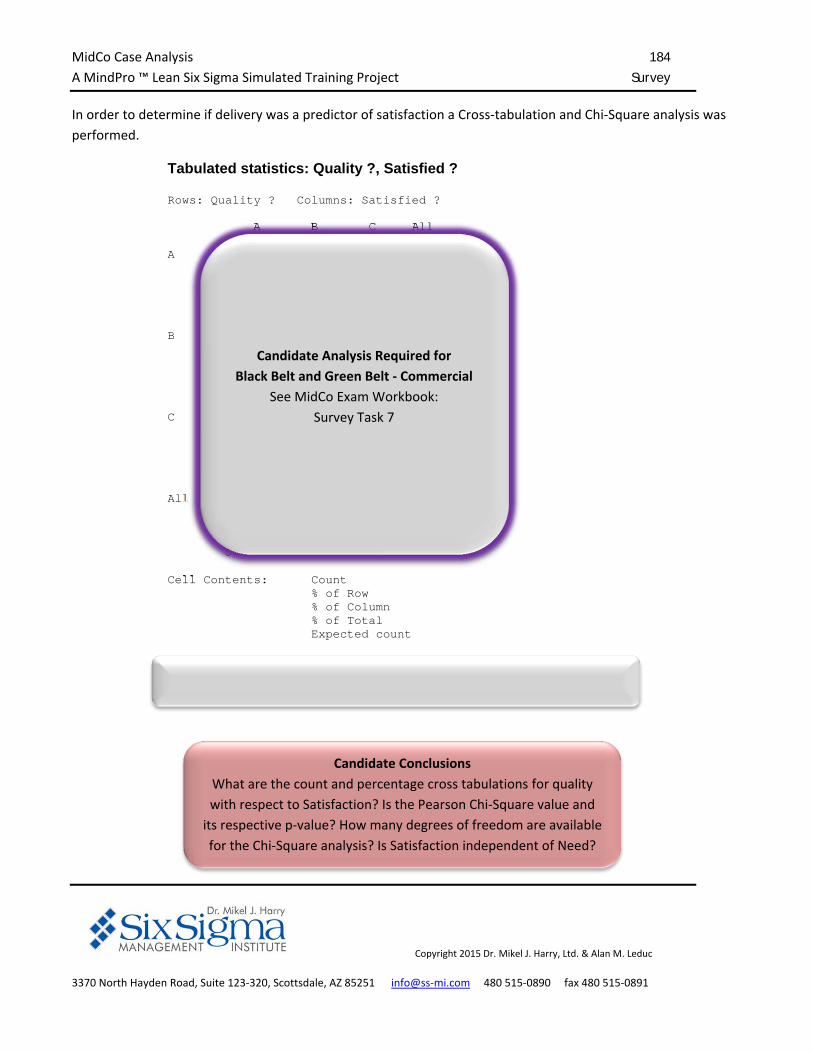
MidCo Case Analysis 184
A MindPro ™ Lean Six Sigma Simulated Training Project Survey
Copyright 2015 Dr. Mikel J. Harry, Ltd. & Alan M. Leduc
3370 North Hayden Road, Suite 123‐320, Scottsdale, AZ 85251 info@ss‐mi.com 480 515‐0890 fax 480 515‐0891
In order to determine if delivery was a predictor of satisfaction a Cross‐tabulation and Chi‐Square analysis was
performed.
Tabulated statistics: Quality ?, Satisfied ? Rows: Quality ? Columns: Satisfied ? A B C All A 0 89 0 89 0.00 100.00 0.00 100.00 0.00 100.00 0.00 44.50 0.00 44.50 0.00 44.50 22.25 39.60 27.15 89.00 B 21 0 31 52 40.38 0.00 59.62 100.00 42.00 0.00 50.82 26.00 10.50 0.00 15.50 26.00 13.00 23.14 15.86 52.00 C 29 0 30 59 49.15 0.00 50.85 100.00 58.00 0.00 49.18 29.50 14.50 0.00 15.00 29.50 14.75 26.25 18.00 59.00 All 50 89 61 200 25.00 44.50 30.50 100.00 100.00 100.00 100.00 100.00 25.00 44.50 30.50 100.00 50.00 89.00 61.00 200.00 Cell Contents: Count % of Row % of Column % of Total Expected count Pearson Chi-Square = 201.547, DF = 4, P-Value = 0.000 Likelihood Ratio Chi-Square = 275.694, DF = 4, P-Value = 0.000
Candidate Analysis Required for
Black Belt and Green Belt ‐ Commercial
See MidCo Exam Workbook:
Survey Task 7
Candidate Conclusions
What are the count and percentage cross tabulations for quality
with respect to Satisfaction? Is the Pearson Chi‐Square value and
its respective p‐value? How many degrees of freedom are available
for the Chi‐Square analysis? Is Satisfaction independent of Need?
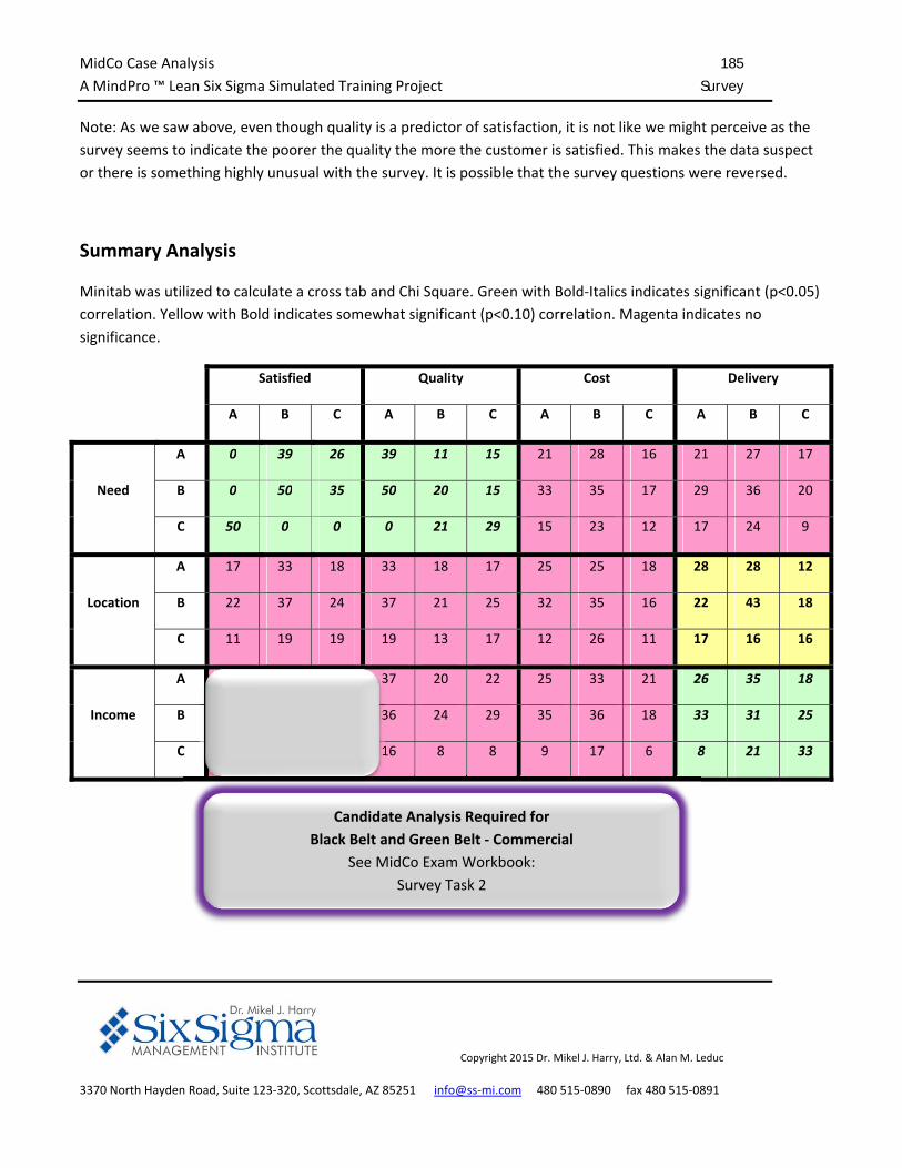
MidCo Case Analysis 185
A MindPro ™ Lean Six Sigma Simulated Training Project Survey
Copyright 2015 Dr. Mikel J. Harry, Ltd. & Alan M. Leduc
3370 North Hayden Road, Suite 123‐320, Scottsdale, AZ 85251 info@ss‐mi.com 480 515‐0890 fax 480 515‐0891
Note: As we saw above, even though quality is a predictor of satisfaction, it is not like we might perceive as the
survey seems to indicate the poorer the quality the more the customer is satisfied. This makes the data suspect
or there is something highly unusual with the survey. It is possible that the survey questions were reversed.
Summary Analysis
Minitab was utilized to calculate a cross tab and Chi Square. Green with Bold‐Italics indicates significant (p<0.05)
correlation. Yellow with Bold indicates somewhat significant (p<0.10) correlation. Magenta indicates no
significance.
Satisfied Quality Cost Delivery
A B C A B C A B C A B C
Need
A 0 39 26 39 11 15 21 28 16 21 27 17
B 0 50 35 50 20 15 33 35 17 29 36 20
C 50 0 0 0 21 29 15 23 12 17 24 9
Location
A 17 33 18 33 18 17 25 25 18 28 28 12
B 22 37 24 37 21 25 32 35 16 22 43 18
C 11 19 19 19 13 17 12 26 11 17 16 16
Income
A 18 37 24 37 20 22 25 33 21 26 35 18
B 25 36 28 36 24 29 35 36 18 33 31 25
C 7 16 9 16 8 8 9 17 6 8 21 33
Candidate Analysis Required for
Black Belt and Green Belt ‐ Commercial
See MidCo Exam Workbook:
Survey Task 2
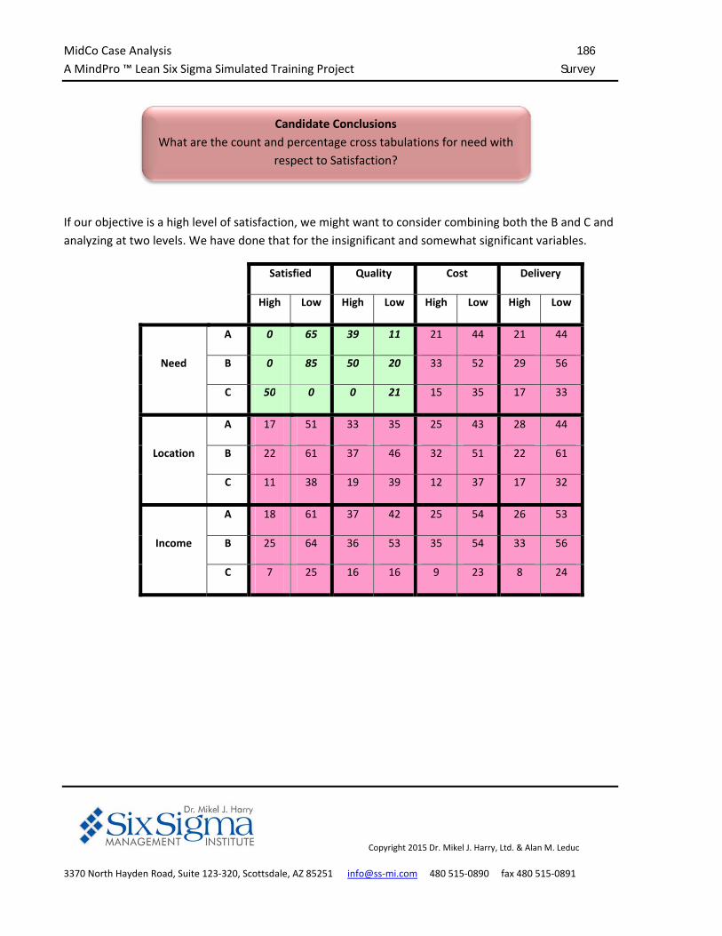
MidCo Case Analysis 186
A MindPro ™ Lean Six Sigma Simulated Training Project Survey
Copyright 2015 Dr. Mikel J. Harry, Ltd. & Alan M. Leduc
3370 North Hayden Road, Suite 123‐320, Scottsdale, AZ 85251 info@ss‐mi.com 480 515‐0890 fax 480 515‐0891
If our objective is a high level of satisfaction, we might want to consider combining both the B and C and
analyzing at two levels. We have done that for the insignificant and somewhat significant variables.
Satisfied Quality Cost Delivery
High Low High Low High Low High Low
Need
A 0 65 39 11 21 44 21 44
B 0 85 50 20 33 52 29 56
C 50 0 0 21 15 35 17 33
Location
A 17 51 33 35 25 43 28 44
B 22 61 37 46 32 51 22 61
C 11 38 19 39 12 37 17 32
Income
A 18 61 37 42 25 54 26 53
B 25 64 36 53 35 54 33 56
C 7 25 16 16 9 23 8 24
Candidate Conclusions
What are the count and percentage cross tabulations for need with
respect to Satisfaction?
MidCo Case Analysis 187
A MindPro ™ Lean Six Sigma Simulated Training Project Survey
Copyright 2015 Dr. Mikel J. Harry, Ltd. & Alan M. Leduc
3370 North Hayden Road, Suite 123‐320, Scottsdale, AZ 85251 info@ss‐mi.com 480 515‐0890 fax 480 515‐0891
Observations
Strong observations:
o Those that have a low need tend to be satisfied overall.
o Those that have a high need tend to be dissatisfied overall.
o Only ¼ of the respondents are highly satisfied overall.
o Those that have a high or moderate need tend to be satisfied with quality.
o Those that have a low need tend to be dissatisfied with quality.
Weak observations:
o Those that have a low income tend to be less satisfied with delivery.
o Those that have a higher income tend to be more satisfied with delivery.
o Location see has a lower number of respondents than the other regions.
o Region B has more dissatisfaction with delivery than the other regions.
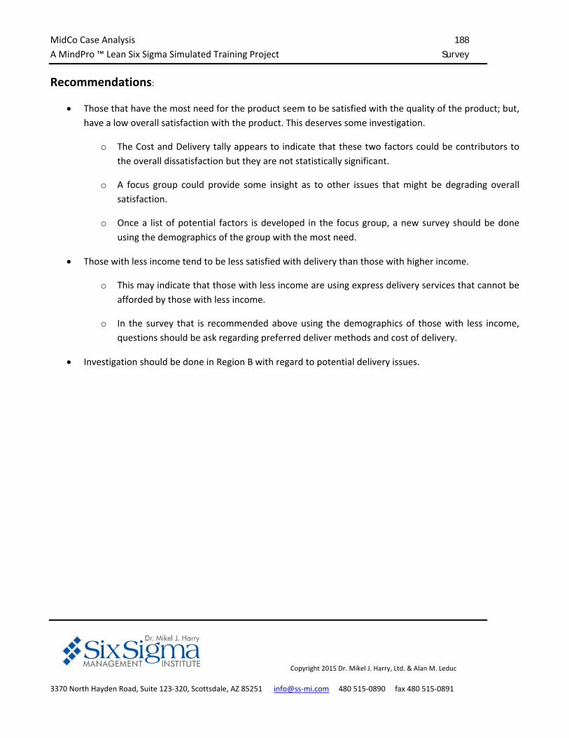
MidCo Case Analysis 188
A MindPro ™ Lean Six Sigma Simulated Training Project Survey
Copyright 2015 Dr. Mikel J. Harry, Ltd. & Alan M. Leduc
3370 North Hayden Road, Suite 123‐320, Scottsdale, AZ 85251 info@ss‐mi.com 480 515‐0890 fax 480 515‐0891
Recommendations:
Those that have the most need for the product seem to be satisfied with the quality of the product; but,
have a low overall satisfaction with the product. This deserves some investigation.
o The Cost and Delivery tally appears to indicate that these two factors could be contributors to
the overall dissatisfaction but they are not statistically significant.
o A focus group could provide some insight as to other issues that might be degrading overall
satisfaction.
o Once a list of potential factors is developed in the focus group, a new survey should be done
using the demographics of the group with the most need.
Those with less income tend to be less satisfied with delivery than those with higher income.
o This may indicate that those with less income are using express delivery services that cannot be
afforded by those with less income.
o In the survey that is recommended above using the demographics of those with less income,
questions should be ask regarding preferred deliver methods and cost of delivery.
Investigation should be done in Region B with regard to potential delivery issues.
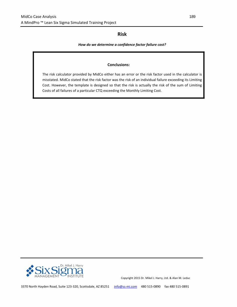
MidCo Case Analysis 189
A MindPro ™ Lean Six Sigma Simulated Training Project
Copyright 2015 Dr. Mikel J. Harry, Ltd. & Alan M. Leduc
3370 North Hayden Road, Suite 123‐320, Scottsdale, AZ 85251 info@ss‐mi.com 480 515‐0890 fax 480 515‐0891
Risk
How do we determine a confidence factor failure cost?
Conclusions:
The risk calculator provided by MidCo either has an error or the risk factor used in the calculator is
misstated. MidCo stated that the risk factor was the risk of an individual failure exceeding its Limiting
Cost. However, the template is designed so that the risk is actually the risk of the sum of Limiting
Costs of all failures of a particular CTQ exceeding the Monthly Limiting Cost.
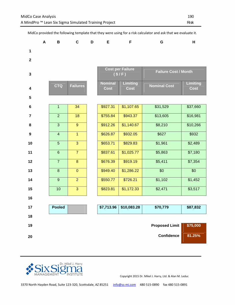
MidCo Case Analysis 190
A MindPro ™ Lean Six Sigma Simulated Training Project Risk
Copyright 2015 Dr. Mikel J. Harry, Ltd. & Alan M. Leduc
3370 North Hayden Road, Suite 123‐320, Scottsdale, AZ 85251 info@ss‐mi.com 480 515‐0890 fax 480 515‐0891
MidCo provided the following template that they were using for a risk calculator and ask that we evaluate it.
A B C D E F G H
1
2
3
Cost per Failure
( $ / F ) Failure Cost / Month
4 CTQ Failures
Nominal
Cost Limiting
Cost Nominal Cost
Limiting Cost
5
6 1 34 $927.31 $1,107.65 $31,529 $37,660
7 2 18 $755.84 $943.37 $13,605 $16,981
8 3 9 $912.26 $1,140.67 $8,210 $10,266
9 4 1 $626.87 $932.05 $627 $932
10 5 3 $653.71 $829.83 $1,961 $2,489
11 6 7 $837.61 $1,025.77 $5,863 $7,180
12 7 8 $676.39 $919.19 $5,411 $7,354
13 8 0 $949.40 $1,286.22 $0 $0
14 9 2 $550.77 $726.21 $1,102 $1,452
15 10 3 $823.81 $1,172.33 $2,471 $3,517
16
17 Pooled $7,713.96 $10,083.28 $70,779 $87,832
18
19 Proposed Limit $75,000
20 Confidence 81.25%
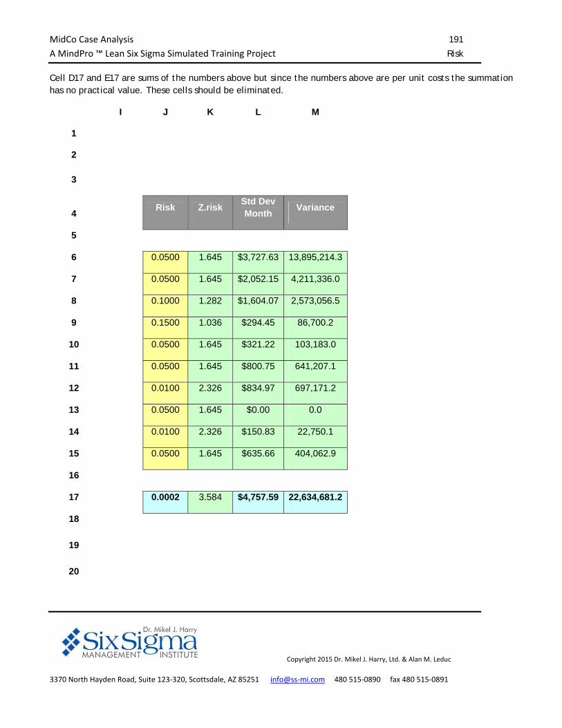
MidCo Case Analysis 191
A MindPro ™ Lean Six Sigma Simulated Training Project Risk
Copyright 2015 Dr. Mikel J. Harry, Ltd. & Alan M. Leduc
3370 North Hayden Road, Suite 123‐320, Scottsdale, AZ 85251 info@ss‐mi.com 480 515‐0890 fax 480 515‐0891
Cell D17 and E17 are sums of the numbers above but since the numbers above are per unit costs the summation has no practical value. These cells should be eliminated.
I J K L M
1
2
3
4 Risk Z.risk
Std DevMonth
Variance
5
6 0.0500 1.645 $3,727.63 13,895,214.3
7 0.0500 1.645 $2,052.15 4,211,336.0
8 0.1000 1.282 $1,604.07 2,573,056.5
9 0.1500 1.036 $294.45 86,700.2
10 0.0500 1.645 $321.22 103,183.0
11 0.0500 1.645 $800.75 641,207.1
12 0.0100 2.326 $834.97 697,171.2
13 0.0500 1.645 $0.00 0.0
14 0.0100 2.326 $150.83 22,750.1
15 0.0500 1.645 $635.66 404,062.9
16
17 0.0002 3.584 $4,757.59 22,634,681.2
18
19
20
MidCo Case Analysis 192
A MindPro ™ Lean Six Sigma Simulated Training Project Risk
Copyright 2015 Dr. Mikel J. Harry, Ltd. & Alan M. Leduc
3370 North Hayden Road, Suite 123‐320, Scottsdale, AZ 85251 info@ss‐mi.com 480 515‐0890 fax 480 515‐0891
MidCo stated that the assumed risk factor (column I) was per failure. However they have pooled as if the risk
factor was the risk of exceeding the limiting cost per month for a particular CTQ. The limiting cost per month
assumes that all individual failures are at the limiting value. This is a grossly conservative assumption. For
example, if there is only a 5% chance of each of the 34 CTQ‐1 failures exceeding the individual limit the risk of all
of the CTQ‐1’s exceeding the overall limit would be 5%^34. This number exceeds the limits of Excel an incorrect
Z.risk value of 8.294, which appears to be the limiting value of the Excel Z table.
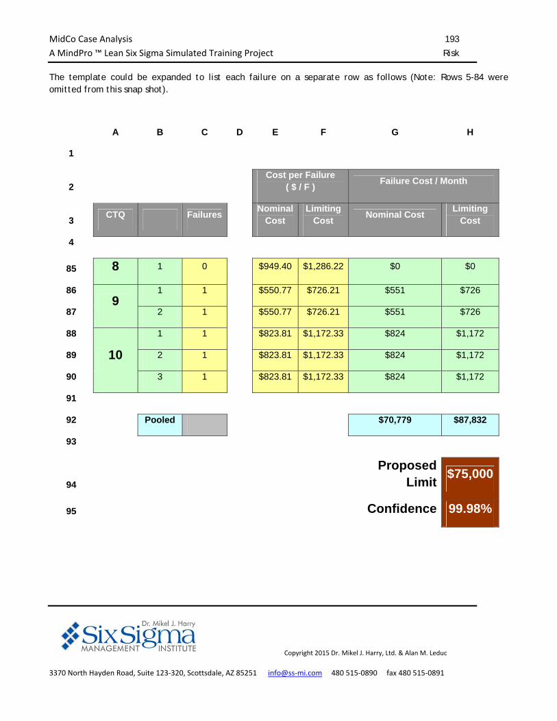
MidCo Case Analysis 193
A MindPro ™ Lean Six Sigma Simulated Training Project Risk
Copyright 2015 Dr. Mikel J. Harry, Ltd. & Alan M. Leduc
3370 North Hayden Road, Suite 123‐320, Scottsdale, AZ 85251 info@ss‐mi.com 480 515‐0890 fax 480 515‐0891
The template could be expanded to list each failure on a separate row as follows (Note: Rows 5-84 were omitted from this snap shot).
A B C D E F G H
1
2
Cost per Failure
( $ / F ) Failure Cost / Month
3 CTQ Failures
Nominal
Cost Limiting
Cost Nominal Cost
Limiting Cost
4
85 8 1 0 $949.40 $1,286.22 $0 $0
86 9
1 1 $550.77 $726.21 $551 $726
87 2 1 $550.77 $726.21 $551 $726
88
10
1 1 $823.81 $1,172.33 $824 $1,172
89 2 1 $823.81 $1,172.33 $824 $1,172
90 3 1 $823.81 $1,172.33 $824 $1,172
91
92 Pooled $70,779 $87,832
93
94
Proposed Limit
$75,000
95 Confidence 99.98%
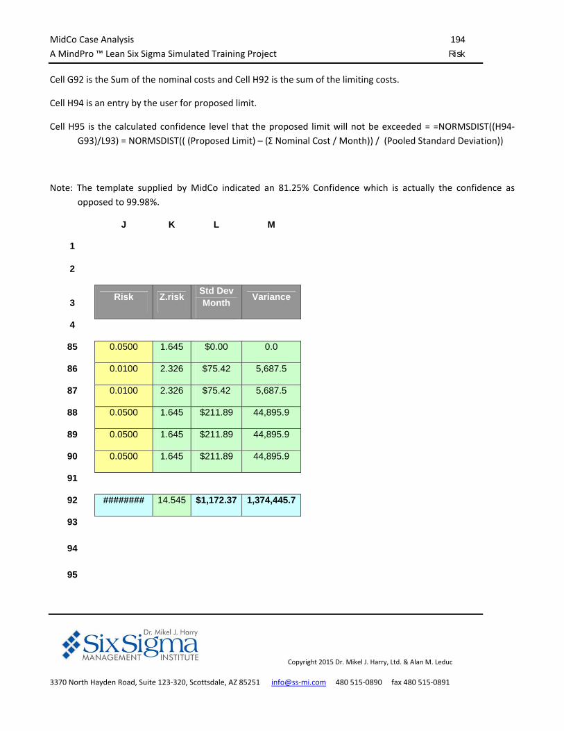
MidCo Case Analysis 194
A MindPro ™ Lean Six Sigma Simulated Training Project Risk
Copyright 2015 Dr. Mikel J. Harry, Ltd. & Alan M. Leduc
3370 North Hayden Road, Suite 123‐320, Scottsdale, AZ 85251 info@ss‐mi.com 480 515‐0890 fax 480 515‐0891
Cell G92 is the Sum of the nominal costs and Cell H92 is the sum of the limiting costs.
Cell H94 is an entry by the user for proposed limit.
Cell H95 is the calculated confidence level that the proposed limit will not be exceeded = =NORMSDIST((H94‐
G93)/L93) = NORMSDIST(( (Proposed Limit) – (Σ Nominal Cost / Month)) / (Pooled Standard Deviation))
Note: The template supplied by MidCo indicated an 81.25% Confidence which is actually the confidence as
opposed to 99.98%.
J K L M
1
2
3 Risk Z.risk
Std DevMonth
Variance
4
85 0.0500 1.645 $0.00 0.0
86 0.0100 2.326 $75.42 5,687.5
87 0.0100 2.326 $75.42 5,687.5
88 0.0500 1.645 $211.89 44,895.9
89 0.0500 1.645 $211.89 44,895.9
90 0.0500 1.645 $211.89 44,895.9
91
92 ######## 14.545 $1,172.37 1,374,445.7
93
94
95
MidCo Case Analysis 195
A MindPro ™ Lean Six Sigma Simulated Training Project Risk
Copyright 2015 Dr. Mikel J. Harry, Ltd. & Alan M. Leduc
3370 North Hayden Road, Suite 123‐320, Scottsdale, AZ 85251 info@ss‐mi.com 480 515‐0890 fax 480 515‐0891
Cell J85 the risk that the individual failure in that row will exceed the limiting cost.
Similarly for J86.J90.
Cell K85 = ‐NORMSINV(J85). Similarly for K85.K90.
Cell L85 =((G85‐F85)/L85)*C85 = ((Limiting Cost – Nominal Cost)/Standard Deviation)*# Failures
Similar for L86.L90.
Cell M85 = L85^2. Similarly for L86.L90.
Cell M92 = Sum(M5.M90)
Cell L92 = M92^.5
Cell K92 = =(I93‐H93)/M93 = ((Sum Limiting Costs – Sum Nominal Costs)/Standard Deviation. = Z.risk that the
cost will exceed that of the sum of the limit costs.
Cell J92 = =1‐NORMSDIST(K92) = The risk that cost will exceed that of the sum of the limit costs.