A Minimum-Delay-Difference Method for MitigatingCross-Traffic Impact on Capacity Measurement

Edmond W. W. Chan‡, Xiapu Luo§, and Rocky K. C. Chang‡

Department of Computing‡ College of Computing§

The Hong Kong Polytechnic University Georgia Institute of Technology{cswwchan|csrchang}@comp.polyu.edu.hk csxpluo@cc.gatech.edu

ABSTRACTThe accuracy and speed of path capacity measurement couldbe seriously affected by the presence of cross traffic on thepath. In this paper, we propose a new cross-traffic filteringmethod called minimum delay difference (MDDIF). Unlikethe classic packet-pair dispersion techniques, the MDDIFmethod can obtain accurate capacity estimate from the min-imal possible delay of packets from different packet pairs.We have proved that the MDDIF method is correct and thatit takes less time to obtain accurate samples than the mini-mum delay sum (MDSUM) method. We also present analyt-ical and measurement results to evaluate the MDDIF methodand to compare its performance with the MDSUM method.

Categories and Subject DescriptorsC.2.3 [Computer-Communication Networks]: Net-work Operations; C.4 [Performance of Systems]: Mea-surement Techniques

General TermsMeasurement, Experimentation, Performance

KeywordsNetwork capacity, Bottleneck bandwidth, Non-cooperativemeasurement, Packet-pair dispersion, Packet delay

1. INTRODUCTIONKnowing network capacity is useful for many net-

work applications to improve their performance. Net-work capacity (a.k.a. bottleneck bandwidth) refers tothe smallest transmission rate of a set of network links,forming a network path from a source to a destination

Permission to make digital or hard copies of all or part of this work forpersonal or classroom use is granted without fee provided that copies arenot made or distributed for profit or commercial advantage and that copiesbear this notice and the full citation on the first page. To copy otherwise, torepublish, to post on servers or to redistribute to lists, requires prior specificpermission and/or a fee.

CoNEXT’09, December 1–4, 2009, Rome, Italy.Copyright 2009 ACM 978-1-60558-636-6/09/12 ...$5.00.

[5]. Measuring capacity is, however, a challenging taskin practice, because the accuracy and speed can be ad-versely affected by cross traffic, packet loss and reorder-ing events, packet sizes, time resolution supported bymeasurement endpoints, probing methods, and others.

Existing capacity measurement tools are mostly ac-tive methods which are based on two main approaches:variable packet size and packet dispersion. The focusof this paper is on the latter approach, in particular,the packet-pair dispersion (PPD) technique that sendsa pair of back-to-back probe packets to measure theirdispersion. The PPD technique could be conducted ina cooperative (e.g., [5, 10]) or non-cooperative manner(e.g., [25, 14, 4]).

The accuracy and speed of the PPD technique, how-ever, could be seriously degraded by the cross trafficpresent on the path under measurement. Therefore, thebasic PPD technique is usually augmented by a com-ponent to filter measurement samples that have beenbiased by cross traffic. A notable example is the mini-mum delay sum (MDSUM) method first introduced toCapProbe [10]. The MDSUM method filters out packetpairs that do not meet a minimum delay sum condition.

However, the existing cross-traffic filtering techniquesstill suffer from slow speed and a large overhead. Ap-plications, such as determining optimal software down-load rates, forming peer-to-peer networks, and estab-lishing multicast trees, will benefit from a fast estima-tion of network capacity [25]. Moreover, injecting alarge amount of probe traffic unnecessarily not only pro-longs the estimation process, but also affects the normaltraffic and introduces additional processing burdens toboth the measuring and remote nodes.

In this paper, we propose a new technique called min-imum delay difference (MDDIF). Unlike the MDSUMmethod that admits a packet pair as the basic unit forcapacity measurement, the MDDIF method admits apacket as a basic unit. The MDDIF method obtainsminimal possible delay of a first probe packet and asecond probe packet, but these two packets do not nec-essarily belong to the same packet pair. By exploiting

205

useful information in a single packet (which is discardedby the MDSUM method), the MDDIF method requiresless time to obtain accurate capacity estimates and hasvery low computation and storage costs.

In §2, we first summarize the existing cross-traffic fil-tering techniques. In §3, we present the model and as-sumptions used throughout this paper and review theclassical PPD technique. We then introduce the MD-DIF method in §4 and compare its performance withthe MDSUM method based on their first passage timesin §5. In §6, we further evaluate the MDDIF method’sperformance based on Internet and testbed experimentresults. We finally conclude this paper in §7.

2. RELATED WORKThere are some apparent similarity between the VPS

techniques [9, 18, 6] and the MDDIF method in termsof requiring minimal possible packet delay. The VPStechniques require the minimal possible delay for a se-quence of variable-sized packets; the MDDIF method,however, requires the minimal possible delay only fora pair of packets with the same size. As a result, theMDDIF method achieves a faster capacity estimationwith a lower storage requirement.

Previous works [24, 22, 5, 25, 10, 4] using packetdispersion for capacity measurement compute capacityestimates by measuring the PPDs based on the inter-arrival time of the two packets or the difference betweenthe two packets’ delay. Although the MDDIF methodalso involves sending packet pairs, it does not measurepacket pairs’ PPDs. Instead, it measures the minimalpossible packet delay for the first and second packets.

Many cross-traffic filtering techniques have been pro-posed in the past. Carter and Crovella propose Bprobe[24] which filters inaccurate estimates using union andintersection of packet-pair measurements with differentpacket sizes. Lai and Baker [15] use a kernel densityestimation method to filter capacity estimates. Pasztorand Veitch [22] analyze several types of components em-bedded in the packet-pair dispersion and select the ca-pacity mode from the high-resolution histogram. Kapooret al. [10] propose the use of the minimum of packet-pairdelay sum to filter distorted dispersion samples.

The packet train dispersion (PTD) technique, on theother hand, performs capacity measurement with thedispersion of a burst of back-to-back probe packets.Pathrate [5] uses both PPD and PTD for capacity mea-surement. DSLprobe [4] exploits the PTD techniquefor capacity measurement and various methods to re-move any cross-traffic interfered spacing between adja-cent packets in the packet train. A most notable prob-lem with the packet train technique is that as the trunklength increases, it is more likely for the packet train tobe affected by cross traffic.

3. MODEL AND PRELIMINARIES

3.1 The modelThis paper considers the capacity measurement sce-

nario in Figure 1. A local endpoint measures the pathcapacity by dispatching a sequence of packet pairs (twoback-to-back packets) to a remote endpoint. Each probepacket elicits a response packet from the remote end-point. The (round-trip) network path under the mea-surement starts from and ends at the local endpoint,consisting of n (where n ≥ 2) hops. The first m hops(where 1 ≤ m < n) belong to the forward path and theremaining n − m hops to the reverse path. The probepackets travel on the forward path; the response packetstravel on the reverse path.

Each hop consists of a (local, remote, or forwarding)node and its outgoing link. We use H(h) (1 ≤ h ≤ n)to denote the hth hop which transmits packets to theoutgoing link with a rate of C(h) bits/second. For con-venience, we label the hops on the path sequentially.Therefore, the local endpoint belongs to H(1), whereasthe remote endpoint belongs to H(m+1). The figure alsoshows a bottleneck link on the forward path which be-longs to a hop denoted by H(hf ). If there are morethan one bottleneck hop on the forward path, H(hf ) isreferred to the one with the largest hf . The above ap-plies similarly to the reverse path, where the bottlenecklink belongs to a hop denoted by H(hr).

There are three types of path capacity metrics: forward-

path capacity (denoted by C(n)f ), reverse-path capacity

(denoted by C(n)r ), and round-trip capacity (denoted by

C(n)b ), where

C(n)f ≡ C(hf ) = min

1≤h≤mC(h).

C(n)r ≡ C(hr) = min

m+1≤h≤nC(h).

C(n)b = min{C

(n)f , C(n)

r }.

3.2 The assumptionsUnless stated otherwise, we adopt the following as-

sumptions in this paper:1. Both the forward and reverse paths are unique and

do not change during the measurement.2. The forwarding node in each hop is a store-and-

forward device using a FIFO queue.3. Each probe packet elicits a single response packet

from the remote endpoint with negligible delay.4. All probe and response packets are received suc-

cessfully. Combining with (1)-(3) also implies thatthe probe packets arrive at the remote endpoint inthe original order, and the response packets arriveat the local endpoint in the original order.

206

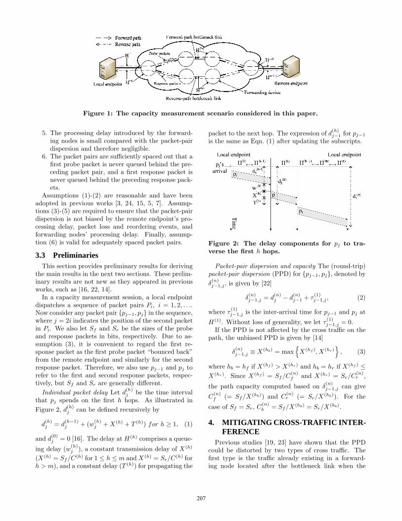
Figure 1: The capacity measurement scenario considered in this paper.

5. The processing delay introduced by the forward-ing nodes is small compared with the packet-pairdispersion and therefore negligible.

6. The packet pairs are sufficiently spaced out that afirst probe packet is never queued behind the pre-ceding packet pair, and a first response packet isnever queued behind the preceding response pack-ets.

Assumptions (1)-(2) are reasonable and have beenadopted in previous works [3, 24, 15, 5, 7]. Assump-tions (3)-(5) are required to ensure that the packet-pairdispersion is not biased by the remote endpoint’s pro-cessing delay, packet loss and reordering events, andforwarding nodes’ processing delay. Finally, assump-tion (6) is valid for adequately spaced packet pairs.

3.3 PreliminariesThis section provides preliminary results for deriving

the main results in the next two sections. These prelim-inary results are not new as they appeared in previousworks, such as [16, 22, 14].

In a capacity measurement session, a local endpointdispatches a sequence of packet pairs Pi, i = 1, 2, . . ..Now consider any packet pair {pj−1, pj} in the sequence,where j = 2i indicates the position of the second packetin Pi. We also let Sf and Sr be the sizes of the probeand response packets in bits, respectively. Due to as-sumption (3), it is convenient to regard the first re-sponse packet as the first probe packet “bounced back”from the remote endpoint and similarly for the secondresponse packet. Therefore, we also use pj−1 and pj torefer to the first and second response packets, respec-tively, but Sf and Sr are generally different.

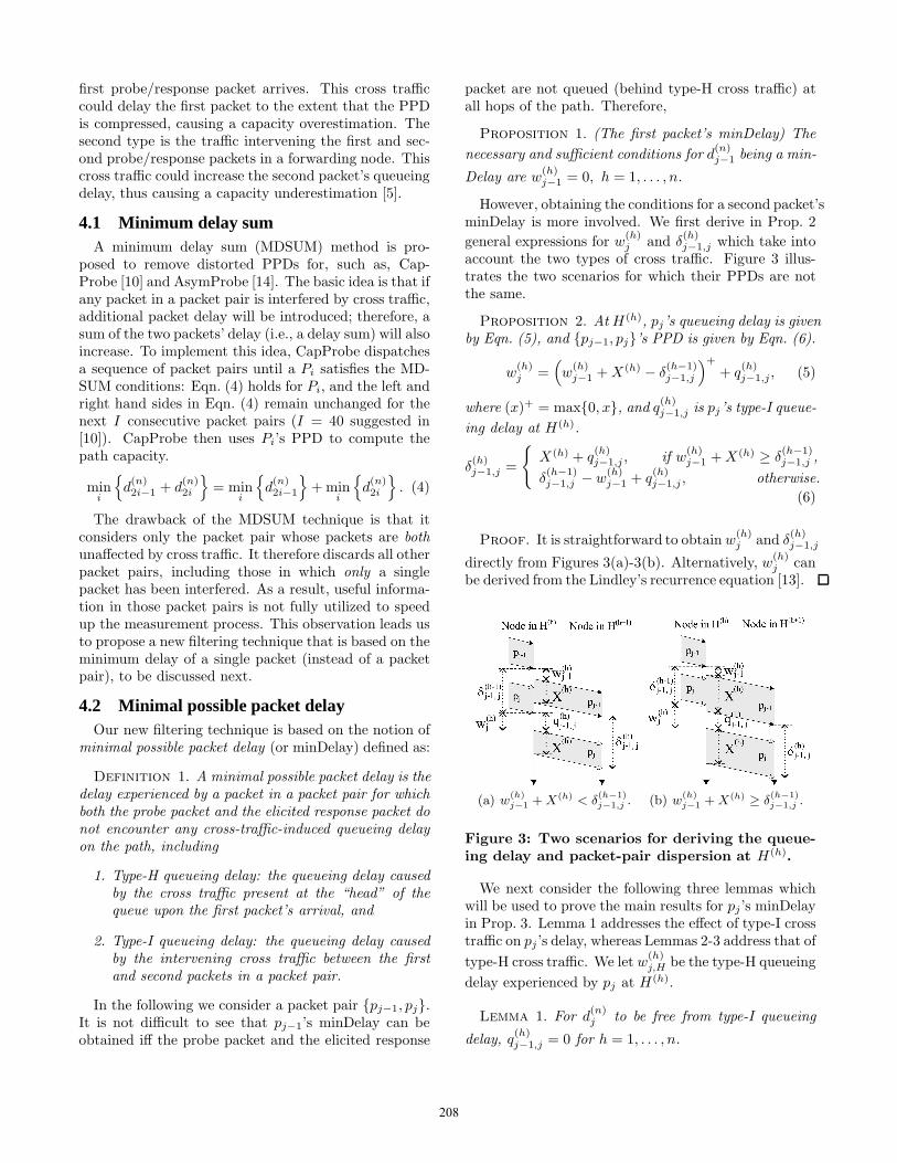
Individual packet delay Let d(h)j be the time interval

that pj spends on the first h hops. As illustrated in

Figure 2, d(h)j can be defined recursively by

d(h)j = d

(h−1)j + (w

(h)j + X(h) + T (h)) for h ≥ 1, (1)

and d(0)j = 0 [16]. The delay at H(h) comprises a queue-

ing delay (w(h)j ), a constant transmission delay of X(h)

(X(h) = Sf/C(h) for 1 ≤ h ≤ m and X(h) = Sr/C(h) forh > m), and a constant delay (T (h)) for propagating the

packet to the next hop. The expression of d(h)j−1 for pj−1

is the same as Eqn. (1) after updating the subscripts.

Figure 2: The delay components for pj to tra-verse the first h hops.

Packet-pair dispersion and capacity The (round-trip)packet-pair dispersion (PPD) for {pj−1, pj}, denoted by

δ(n)j−1,j , is given by [22]

δ(n)j−1,j = d

(n)j − d

(n)j−1 + τ

(1)j−1,j , (2)

where τ(1)j−1,j is the inter-arrival time for pj−1 and pj at

H(1). Without loss of generality, we let τ(1)j−1,j = 0.

If the PPD is not affected by the cross traffic on thepath, the unbiased PPD is given by [14]

δ(n)j−1,j ≡ X(hb) = max

{

X(hf), X(hr)}

, (3)

where hb = hf if X(hf) > X(hr) and hb = hr if X(hf ) ≤

X(hr). Since X(hf ) = Sf/C(n)f and X(hr) = Sr/C

(n)r ,

the path capacity computed based on δ(n)j−1,j can give

C(n)f (= Sf/X(hb)) and C

(n)r (= Sr/X(hb)). For the

case of Sf = Sr, C(n)b = Sf/X(hb) = Sr/X(hb).

4. MITIGATING CROSS-TRAFFIC INTER-FERENCE

Previous studies [19, 23] have shown that the PPDcould be distorted by two types of cross traffic. Thefirst type is the traffic already existing in a forward-ing node located after the bottleneck link when the

207

first probe/response packet arrives. This cross trafficcould delay the first packet to the extent that the PPDis compressed, causing a capacity overestimation. Thesecond type is the traffic intervening the first and sec-ond probe/response packets in a forwarding node. Thiscross traffic could increase the second packet’s queueingdelay, thus causing a capacity underestimation [5].

4.1 Minimum delay sumA minimum delay sum (MDSUM) method is pro-

posed to remove distorted PPDs for, such as, Cap-Probe [10] and AsymProbe [14]. The basic idea is that ifany packet in a packet pair is interfered by cross traffic,additional packet delay will be introduced; therefore, asum of the two packets’ delay (i.e., a delay sum) will alsoincrease. To implement this idea, CapProbe dispatchesa sequence of packet pairs until a Pi satisfies the MD-SUM conditions: Eqn. (4) holds for Pi, and the left andright hand sides in Eqn. (4) remain unchanged for thenext I consecutive packet pairs (I = 40 suggested in[10]). CapProbe then uses Pi’s PPD to compute thepath capacity.

mini

{

d(n)2i−1 + d

(n)2i

}

= mini

{

d(n)2i−1

}

+ mini

{

d(n)2i

}

. (4)

The drawback of the MDSUM technique is that itconsiders only the packet pair whose packets are bothunaffected by cross traffic. It therefore discards all otherpacket pairs, including those in which only a singlepacket has been interfered. As a result, useful informa-tion in those packet pairs is not fully utilized to speedup the measurement process. This observation leads usto propose a new filtering technique that is based on theminimum delay of a single packet (instead of a packetpair), to be discussed next.

4.2 Minimal possible packet delayOur new filtering technique is based on the notion of

minimal possible packet delay (or minDelay) defined as:

Definition 1. A minimal possible packet delay is thedelay experienced by a packet in a packet pair for whichboth the probe packet and the elicited response packet donot encounter any cross-traffic-induced queueing delayon the path, including

1. Type-H queueing delay: the queueing delay causedby the cross traffic present at the “head” of thequeue upon the first packet’s arrival, and

2. Type-I queueing delay: the queueing delay causedby the intervening cross traffic between the firstand second packets in a packet pair.

In the following we consider a packet pair {pj−1, pj}.It is not difficult to see that pj−1’s minDelay can beobtained iff the probe packet and the elicited response

packet are not queued (behind type-H cross traffic) atall hops of the path. Therefore,

Proposition 1. (The first packet’s minDelay) The

necessary and sufficient conditions for d(n)j−1 being a min-

Delay are w(h)j−1 = 0, h = 1, . . . , n.

However, obtaining the conditions for a second packet’sminDelay is more involved. We first derive in Prop. 2

general expressions for w(h)j and δ

(h)j−1,j which take into

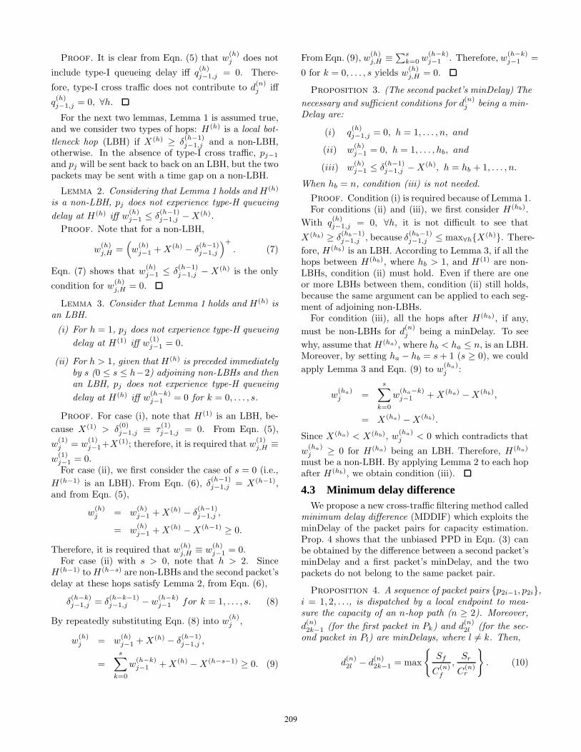
account the two types of cross traffic. Figure 3 illus-trates the two scenarios for which their PPDs are notthe same.

Proposition 2. At H(h), pj’s queueing delay is givenby Eqn. (5), and {pj−1, pj}’s PPD is given by Eqn. (6).

w(h)j =

(

w(h)j−1 + X(h) − δ

(h−1)j−1,j

)+

+ q(h)j−1,j , (5)

where (x)+ = max{0, x}, and q(h)j−1,j is pj’s type-I queue-

ing delay at H(h).

δ(h)j−1,j =

{

X(h) + q(h)j−1,j , if w

(h)j−1 + X(h) ≥ δ

(h−1)j−1,j ,

δ(h−1)j−1,j − w

(h)j−1 + q

(h)j−1,j , otherwise.

(6)

Proof. It is straightforward to obtain w(h)j and δ

(h)j−1,j

directly from Figures 3(a)-3(b). Alternatively, w(h)j can

be derived from the Lindley’s recurrence equation [13].

(a) w(h)j−1 + X(h) < δ

(h−1)j−1,j . (b) w

(h)j−1 + X(h)

≥ δ(h−1)j−1,j .

Figure 3: Two scenarios for deriving the queue-ing delay and packet-pair dispersion at H(h).

We next consider the following three lemmas whichwill be used to prove the main results for pj’s minDelayin Prop. 3. Lemma 1 addresses the effect of type-I crosstraffic on pj ’s delay, whereas Lemmas 2-3 address that of

type-H cross traffic. We let w(h)j,H be the type-H queueing

delay experienced by pj at H(h).

Lemma 1. For d(n)j to be free from type-I queueing

delay, q(h)j−1,j = 0 for h = 1, . . . , n.

208

Proof. It is clear from Eqn. (5) that w(h)j does not

include type-I queueing delay iff q(h)j−1,j = 0. There-

fore, type-I cross traffic does not contribute to d(n)j iff

q(h)j−1,j = 0, ∀h.

For the next two lemmas, Lemma 1 is assumed true,and we consider two types of hops: H(h) is a local bot-

tleneck hop (LBH) if X(h) ≥ δ(h−1)j−1,j and a non-LBH,

otherwise. In the absence of type-I cross traffic, pj−1

and pj will be sent back to back on an LBH, but the twopackets may be sent with a time gap on a non-LBH.

Lemma 2. Considering that Lemma 1 holds and H(h)

is a non-LBH, pj does not experience type-H queueing

delay at H(h) iff w(h)j−1 ≤ δ

(h−1)j−1,j − X(h).

Proof. Note that for a non-LBH,

w(h)j,H =

(

w(h)j−1 + X(h) − δ

(h−1)j−1,j

)+

. (7)

Eqn. (7) shows that w(h)j−1 ≤ δ

(h−1)j−1,j − X(h) is the only

condition for w(h)j,H = 0.

Lemma 3. Consider that Lemma 1 holds and H(h) isan LBH.

(i) For h = 1, pj does not experience type-H queueing

delay at H(1) iff w(1)j−1 = 0.

(ii) For h > 1, given that H(h) is preceded immediatelyby s (0 ≤ s ≤ h−2) adjoining non-LBHs and thenan LBH, pj does not experience type-H queueing

delay at H(h) iff w(h−k)j−1 = 0 for k = 0, . . . , s.

Proof. For case (i), note that H(1) is an LBH, be-

cause X(1) > δ(0)j−1,j ≡ τ

(1)j−1,j = 0. From Eqn. (5),

w(1)j = w

(1)j−1+X(1); therefore, it is required that w

(1)j,H ≡

w(1)j−1 = 0.For case (ii), we first consider the case of s = 0 (i.e.,

H(h−1) is an LBH). From Eqn. (6), δ(h−1)j−1,j = X(h−1),

and from Eqn. (5),

w(h)j = w

(h)j−1 + X(h) − δ

(h−1)j−1,j ,

= w(h)j−1 + X(h) − X(h−1) ≥ 0.

Therefore, it is required that w(h)j,H ≡ w

(h)j−1 = 0.

For case (ii) with s > 0, note that h > 2. SinceH(h−1) to H(h−s) are non-LBHs and the second packet’sdelay at these hops satisfy Lemma 2, from Eqn. (6),

δ(h−k)j−1,j = δ

(h−k−1)j−1,j − w

(h−k)j−1 for k = 1, . . . , s. (8)

By repeatedly substituting Eqn. (8) into w(h)j ,

w(h)j = w

(h)j−1 + X(h) − δ

(h−1)j−1,j ,

=

s∑

k=0

w(h−k)j−1 + X(h) − X(h−s−1) ≥ 0. (9)

From Eqn. (9), w(h)j,H ≡

∑sk=0 w

(h−k)j−1 . Therefore, w

(h−k)j−1 =

0 for k = 0, . . . , s yields w(h)j,H = 0.

Proposition 3. (The second packet’s minDelay) The

necessary and sufficient conditions for d(n)j being a min-

Delay are:

(i) q(h)j−1,j = 0, h = 1, . . . , n, and

(ii) w(h)j−1 = 0, h = 1, . . . , hb, and

(iii) w(h)j−1 ≤ δ

(h−1)j−1,j − X(h), h = hb + 1, . . . , n.

When hb = n, condition (iii) is not needed.

Proof. Condition (i) is required because of Lemma 1.For conditions (ii) and (iii), we first consider H(hb).

With q(h)j−1,j = 0, ∀h, it is not difficult to see that

X(hb) ≥ δ(hb−1)j−1,j , because δ

(hb−1)j−1,j ≤ max∀h{X

(h)}. There-

fore, H(hb) is an LBH. According to Lemma 3, if all thehops between H(hb), where hb > 1, and H(1) are non-LBHs, condition (ii) must hold. Even if there are oneor more LBHs between them, condition (ii) still holds,because the same argument can be applied to each seg-ment of adjoining non-LBHs.

For condition (iii), all the hops after H(hb), if any,

must be non-LBHs for d(n)j being a minDelay. To see

why, assume that H(ha), where hb < ha ≤ n, is an LBH.Moreover, by setting ha − hb = s + 1 (s ≥ 0), we could

apply Lemma 3 and Eqn. (9) to w(ha)j :

w(ha)j =

s∑

k=0

w(ha−k)j−1 + X(ha) − X(hb),

= X(ha) − X(hb).

Since X(ha) < X(hb), w(ha)j < 0 which contradicts that

w(ha)j ≥ 0 for H(ha) being an LBH. Therefore, H(ha)

must be a non-LBH. By applying Lemma 2 to each hopafter H(hb), we obtain condition (iii).

4.3 Minimum delay differenceWe propose a new cross-traffic filtering method called

minimum delay difference (MDDIF) which exploits theminDelay of the packet pairs for capacity estimation.Prop. 4 shows that the unbiased PPD in Eqn. (3) canbe obtained by the difference between a second packet’sminDelay and a first packet’s minDelay, and the twopackets do not belong to the same packet pair.

Proposition 4. A sequence of packet pairs {p2i−1, p2i},i = 1, 2, . . ., is dispatched by a local endpoint to mea-sure the capacity of an n-hop path (n ≥ 2). Moreover,

d(n)2k−1 (for the first packet in Pk) and d

(n)2l (for the sec-

ond packet in Pl) are minDelays, where l 6= k. Then,

d(n)2l − d

(n)2k−1 = max

{

Sf

C(n)f

,Sr

C(n)r

}

. (10)

209

Proof. First of all, from Eqn. (1),

d(n)2l − d

(n)2k−1 = w

(n)2l − w

(n)2k−1 + d

(n−1)2l − d

(n−1)2k−1 . (11)

Using w(n)2k−1 = 0 (from Prop. 1), Eqn. (5) for w

(n)2l , and

q(n)2l−1,2l = 0 (from Prop. 3(i)), Eqn. (11) becomes

d(n)2l − d

(n)2k−1 = d

(n−1)2l − d

(n−1)2k−1 +

(

w(n)2l−1 + X(n) − δ

(n−1)2l−1,2l

)+

.(12)

We now use mathematical induction on n for the proof.The base case: n = 2 (i.e., hf = 1 and hr = 2) Byapplying Eqn. (12) recursively for n = 2, we obtain

d(2)2l − d

(2)2k−1 =

2∑

h=1

(

w(h)2l−1 + X(h) − δ

(h−1)2l−1,2l

)+

. (13)

Note that δ(0)2l−1,2l ≡ τ

(1)2l−1,2l = 0. Moreover, H(hb) is

either H(1) (the forward-path hop) or H(2) (the reverse-path hop):

Case 1 (hb = hf = 1): Since d(2)2l is a minDelay, w

(1)2l−1 =

0 (from Prop. 3(ii)) and(

w(2)2l−1 + X(2) − δ

(1)2l−1,2l

)+

= 0

(from Prop. 3(iii)). Eqn. (13) therefore becomes

d(2)2l − d

(2)2k−1 = X(1) = Sf/C(1),

which is the same as Eqn. (10) for n = 2.

Case 2 (hb = hr = 2): Since d(2)2l is a minDelay, w

(1)2l−1 =

w(2)2l−1 = 0 (from Prop. 3(ii)) and δ

(1)2l−1,2l = X(1). Eqn. (13)

therefore becomes

d(2)2l − d

(2)2k−1 = X(2) = Sr/C(2),

which is the same as Eqn. (10) for n = 2.The inductive step: Assuming that Eqn. (10) holds forn ≥ 2, we prove that Eqn. (10) also holds for n + 1. Bysubstituting Eqn. (10) (the inductive hypothesis for n)into Eqn. (12) for n + 1, we have

d(n+1)2l − d

(n+1)2k−1 =

(

w(n+1)2l−1 + X(n+1) − δ

(n)2l−1,2l

)+

,

+ max{

Sf/C(n)f , Sr/C(n)

r

}

. (14)

There are two cases to consider: hb remains the same,and hb = n+1. Note that H(n+1) introduces a new linkto the reverse path.

Case 1 (hb < n + 1): Since d(n+1)2l is a minDelay, ap-

plying w(n+1)2l−1 ≤ δ

(n)2l−1,2l −X(n+1) (from Prop. 3(iii)) to

Eqn. (14) yields

d(n+1)2l − d

(n+1)2k−1 = max

{

Sf/C(n)f , Sr/C(n)

r

}

,

= max{

Sf/C(n+1)f , Sr/C(n+1)

r

}

.

(15)

Case 2 (hb = n + 1): Since d(n+1)2l is a minDelay, we

have w(h)2l−1 = 0, ∀1 ≤ h ≤ n + 1 (from Prop. 3(ii)).

Accordingly, both d(n)2l and d

(n)2l−1 are also minDelays;

therefore, d(n)2l − d

(n)2l−1 = max

{

Sf/C(n)f , Sr/C

(n)r

}

(the

inductive hypothesis). Substituting w(n+1)2l−1 = 0 and

δ(n)2l−1,2l = d

(n)2l − d

(n)2l−1 (from Eqn. (2)) into Eqn. (14)

yields

d(n+1)2l − d

(n+1)2k−1 = X(n+1) = Sr/C(n+1),

which is the same as Eqn. (15).

5. A FIRST-PASSAGE-TIME ANALYSIS OFTHE MDDIF AND MDSUM METHODS

In this section, we analyze and compare the MD-DIF and MDSUM methods based on their first passagetimes. The MDDIF method’s first passage time (FPT)is defined as the first time (in terms of the number ofpacket pairs sent) to obtain the two minDelays. On theother hand, the MDSUM method’s FPT is defined asthe first time to obtain the minimum delay sum (whichis equal to the sum of the two minDelays). Therefore,a smaller FPT results in a faster measurement. More-over, we consider a multi-hop path scenario, instead ofa single-hop model considered in [10].

5.1 The first passage timeLet Xi, i ≥ 1, be a sequence of independent and iden-

tically distributed (i.i.d.) Bernoulli random variableswith parameter pX (probability for Xi = 1) for theminDelay event of p2i−1 (the first packet in Pi). Xi = 1

if d(n)2i−1 is a minDelay and Xi = 0, otherwise. Similarly,

Yi, i ≥ 1, is a sequence of i.i.d. Bernoulli random vari-ables with parameter pY for the minDelay event of p2i

(the second packet in Pi). Yi = 1 if d(n)2i is a minDe-

lay and Yi = 0, otherwise. Moreover, the sequence ofthe joint random variables (Xi, Yi) are i.i.d. with a jointprobability density function (pdf) pXY (x, y). Note thatXi and Yi are generally not independent.

The MDDIF method’s FPT is given by

TDIF = inf{i : SXi > 0 and SYi > 0}, (16)

where SXi =∑i

k=1 Xk and SYi =∑i

k=1 Yk. To ob-tain the pdf for TDIF , we consider another sequence ofrandom variables Zi, i ≥ 1, for which

Zi =

0, if SXi = 0 and SYi = 0,1, if SXi = 0 and SYi > 0,2, if SXi > 0 and SYi = 0,3, if SXi > 0 and SYi > 0,

is a time-homogeneous Markov chain with transient states0, 1, and 2, and an absorbing state 3. Denote the sta-tionary transition probabilities by pmn = P [Zi+1 =n|Zi = m], m, n = 0, 1, 2, 3, and the transition prob-

210

ability matrix P of the Markov chain by

P = [pmn],

=

[

Q A0 1

]

,

=

pXY (0, 0) pXY (0, 1) pXY (1, 0) pXY (1, 1)0 1 − pX 0 pX

0 0 1 − pY pY

0 0 0 1

,

where Q is for the transitions among the three tran-sient states, whereas A is for the transitions from thetransient states to the absorbing state. Since the MD-DIF method starts from state 0, the initial probabilityvector for the first three (transient) states is given byπ0 = [1 0 0]. From [20],

P [TDIF = i] = π0Qi−1A. (17)

To determine the expectation of the FPT, we obtaint = [t0, t1, t2]

T , for which tk, k = 0, 1, 2, is the expectednumber of steps taken prior to reaching the absorbingstate, given that the chain begins from state k. From[12], t = (I − Q)−1c, where I is an identity matrix,c = [1 1 1]T , and (I − Q)−1 is the fundamental matrixof the Markov chain. We therefore have

E[TDIF ] = π0t,

=

(

1

1 − pXY (0, 0)

) (

1 +pXY (0, 1)

pX

+pXY (1, 0)

pY

)

.

(18)

On the other hand, the MDSUM method’s FPT isdefined as

TSUM = inf{i : Xi = 1 and Yi = 1}. (19)

Therefore, TSUM is a geometrically distributed randomvariable with parameter pXY (1, 1).

Besides showing that E[TDIF ] < E[TSUM ], Prop. 5also states the main idea of the MDDIF method. Thenecessary and sufficient condition for the MDDIF methodto obtain capacity estimates faster than the MDSUMmethod is when it is possible to find the two minDe-lays from different packet pairs (i.e., pXY (0, 1) > 0 andpXY (1, 0) > 0).

Proposition 5. E[TDIF ] < E[TSUM ] iff pXY (0, 1) >0 and pXY (1, 0) > 0.

Proof. By using Eqn. (18) and E[TSUM ] = 1/pXY (1, 1),we compute the relative gain of E[TDIF ] as

Ψ =E[TSUM ] − E[TDIF ]

E[TSUM ]=

σ

σ + ξ, (20)

where

σ = pXY (0, 1)pXY (1, 0)(pX + pY ), (21)

ξ = pXY (1, 1)[pXY (0, 1)(pX + pY ) + p2X ]. (22)

Assume that pXY (0, 1) > 0 and pXY (1, 0) > 0. SincepX = pXY (1, 0)+pXY (1, 1), pXY (1, 0) > 0 implies pX >0. Similarly, pXY (0, 1) > 0 implies pY > 0. FromEqn. (21), σ > 0. Moreover, 0 ≤ pXY (1, 1) < 1 due tothe law of total probability, and it is easy to see that0 < [pXY (0, 1)(pX+pY )+p2

X ] < 1. Therefore, 0 ≤ ξ < 1from Eqn. (22), and as a result, 0 < Ψ ≤ 1.

In the other direction, assume that Ψ > 0. FromEqns. (20)-(21), pXY (0, 1)pXY (1, 0)(pX+pY ) > 0 whichis equivalent to pXY (0, 1) > 0 and pXY (1, 0) > 0.

Prop. 6 shows that the MDDIF method does not havethe speed advantage for hb = n. Since H(n) is a reverse-path hop, the MDDIF and MDSUM methods give the

same expected FPTs for measuring C(n)r . Nevertheless,

the MDDIF method’s speed advantage may still be re-

tained for measuring C(n)f if Sf and Sr are selected such

that hb = hf . This could be done for C(n)r ≥ C

(n)f

(e.g., by choosing Sf = Sr), and for C(n)r < C

(n)f if it

is feasible to achieve Sf/Sr > C(n)f /C

(n)r > 1 (see the

discussion for Eqn. (3)).

Proposition 6. E[TDIF ] = E[TSUM ] for hb = n.

Proof. The event of Xi = 0 and Yi = 1 is not possi-ble (i.e., pXY (0, 1) = 0) for this scenario. Since p2i−1 is

not a minDelay, w(h)2i−1 6= 0 for some h (from Prop. 1).

Thus, it is not possible for p2i being a minDelay, because

w(h)2i−1 = 0 is required for all h (according to Prop. 3).

As a result, σ = 0 in Eqn. (21); thus, Ψ = 0.

5.2 A first-passage-time analysis forhb = n− 1

To quantify the MDDIF method’s speed advantagefor hb 6= n, we analyze the case of hb = n − 1 here.We model the node in H(h) as a single FIFO queuewith unlimited buffer. The packet inter-arrival timesfor the cross traffic to the queue at H(h) (denoted byA(h)) are exponentially distributed with rate λ(h). Thisassumption is based on the previous study that thecross traffic distribution is reasonably represented bythe Poisson process on sub-second timescales [11]. Theinter-arrival process for the packet pairs to the queue isalso exponential; therefore, they take a random look atthe state of the queue. Since the packet pairs do notgenerate a significant load to H(n), the average packetarrival rate λ(h) is retained. The packet service timeat H(h) (denoted by B(h)) is a random variable whichdepends on the packet size (denoted by S(h)) distribu-tion and C(h). To make the analysis simple, we as-sume that B(h) is an exponential random variable withµ(h) = 1/E[B(h)] = C(h)/E[S(h)] being the packet ser-vice rate at H(h). As a result, each node is modeled asa classic M/M/1 queue.

211

5.2.1 Computing the probabilities

In this section we derive analytical expressions forthe probabilities in Eqn. (18) for the MDDIF methodand pXY (1, 1) for the MDSUM method. We also notethat it is sufficient to obtain expressions for pXY (1, 1),pX , and pY , because they can be used to obtain otherprobabilities.

Computing pX We again consider {pj−1, pj}. Sincepj will not affect pj−1, pX is the probability that allnodes on the path are empty upon pj−1’s arrival. Theempty probability is given by 1− ρ(h) for H(h) [20]. Byapplying an independence assumption for the nodes,

pX =

n∏

h=1

(

1 − ρ(h))

, (23)

where ρ(h) = λ(h)/µ(h).Computing pXY (1, 1) Same as the last case, pj−1 ar-

rives at an empty node in H(h) with probability 1−ρ(h).Given that a period of t has been passed since the lastcross-traffic packet arrival upon pj−1’s arrival at H(h),the probability that pj will not be delayed by the in-tervening cross traffic between pj−1 and pj is given by

P [A(h) > t + δ(h−1)j−1,j |A

(h) > t]. By the memorylessproperty of an exponential distribution, this conditional

probability is given by P [A(h) > δ(h−1)j−1,j ] = e−λ(h)δ

(h−1)j−1,j .

Hence,

pXY (1, 1) =

n∏

h=1

(

1 − ρ(h))

e−λ(h)δ(h−1)j−1,j . (24)

Computing pY Since hb = n − 1, we consider twosubpaths for the analysis: (i) {H(1), . . . , H(n−1)} and(ii) {H(n)}. Let p′Y be the probability that pj’s delayon subpath (i) is a minDelay and p′′Y the probabilitythat pj ’s delay on subpath (ii) is a minDelay. Therefore,pY = p′Y p′′Y .

For subpath (i), due to Prop. 3(i)-(ii), both pj−1 andpj do not experience queueing delay on the subpath.Therefore, p′Y is the same as Eqn. (24) except for thelast hop.

The subpath (ii) consists of H(n) which is after H(hb).Therefore, according to Prop. 3(iii), pj−1 must not be

delayed by more than ω = δ(n−1)j−1,j − X(n) > 0. Let

W (n) be the random variable for pj−1’s queueing delayat H(n). Based on the Pollaczek-Khinchin equation foran M/M/1 queue [20],

pW (n)(t) =(

1 − ρ(n))(

δ0(t) + λ(n)e−µ(n)(1−ρ(n))t)

,

(25)where δ0(t) is the Dirac delta function. Moreover, pj

does not encounter intervening cross traffic at H(n) (fromProp. 3(i)). The probability for this event, conditionedon the event that pj−1 has encountered a queueing de-lay of t, is given by the probability of the event A(n) >

δ(n−1)j−1,j − t. Therefore, we can obtain p′′Y and pY :

p′′Y =

∫ ω

0

P [W (n) = t, A(n) > δ(n−1)j−1,j − t]dt,

= (1 − ρ(n))e−λ(n)δ(n−1)j−1,j

[

1 +ρ(n)

1 − 2ρ(n)

×(

1 − e−µ(n)(1−2ρ(n))ω)]

, (26)

pY = p′Y p′′Y ,

= pXY (1, 1)

[

1 +ρ(n)

1 − 2ρ(n)

(

1 − e−µ(n)(1−2ρ(n))ω)

]

.

(27)

5.2.2 Analytical results

Using the analytical results from the last section forhb = n − 1, Figure 4 reports Ψ for n = 5 with link ca-pacities of {100, 75, 55, 40, 80} Mbits/s and Sf = {240,576, 1500} bytes. Each sub-figure plots Ψ against amean utilization ρ (ρ(h) = ρ, ∀h) with a given mean(cross-traffic) packet size Sc (E[S(h)] = Sc, ∀h). Theresults are in agreement with Prop. 5.

Figure 4 shows that the benefit of the MDDIF methodincreases with Sf and ρ, but decreases with Sc. Asρ increases, pX , pXY (1, 1), pY , pXY (0, 1) all decrease(Eqns. (23) (24), (27), and (28)). That is, it is harderfor both MDDIF and MDSUM methods to find validsamples as the intensity of cross traffic increases. How-ever, the impact on the MDSUM method is much moreserious, because it is required to obtain the minDelayfor both packets from the same packet pair.

As for the impact of Sf and Sc, Figure 5(a) shows thedistribution of pXY (1, 1) with Sc = [240, 1500] bytes,Sf = Sr = [240, 1500] bytes, and ρ = 20%. Notice thatpXY (1, 1) drops drastically as Sf increases and Sc de-creases, causing the MDSUM method a longer time tofind a valid capacity sample. This is because the PPD

(δ(hb)j−1,j) increases with Sf and the probability for the

cross-traffic packets intervening between the two pack-ets increases for a small Sc. Although Sf and Sc also af-fect the MDDIF method in a similar fashion, the impactis less severe, because it can obtain the two minDelaysfrom different packet pairs.

There is also a subtle relationship between Sf andSc concerning pXY (0, 1), which is illustrated in Figure5(b). By inspecting Eqn. (27),

pXY (0, 1) =pXY (1, 1)ρ(n)

1 − 2ρ(n)

(

1 − e−µ(n)(1−2ρ(n))ω)

.

(28)

Clearly, the likelihood of fulfilling Prop. 3(iii) increaseswith Sf , because the probability of pj ’s queueing dueto pj−1’s decreases. Increasing Sf , however, can de-crease the probability of fulfilling Prop. 3(i), becausethe increased dispersion can accommodate more cross-

212

0 0.2 0.4 0.6 0.8 10

0.2

0.4

0.6

0.8

1

ρ

Ψ

Sc=240 bytes

Sc=576 bytes

Sc=1500 bytes

(a) Sf = 240 bytes.

0 0.2 0.4 0.6 0.8 10

0.2

0.4

0.6

0.8

1

ρ

Ψ

Sc=240 bytes

Sc=576 bytes

Sc=1500 bytes

(b) Sf = 576 bytes.

0 0.2 0.4 0.6 0.8 10

0.2

0.4

0.6

0.8

1

ρ

Ψ

Sc=240 bytes

Sc=576 bytes

Sc=1500 bytes

(c) Sf = 1500 bytes.

Figure 4: The relative gain of the expected first passage times for the MDDIF and MDSUM methods.

0500

10001500

0500

10001500

00.10.20.30.4

Sf (bytes)S

c (bytes)

pX

Y(1

,1)

(a) pXY (1, 1).

0500

10001500

0500

10001500

00.010.020.030.04

Sf (bytes)S

c (bytes)

pX

Y(0

,1)

(b) pXY (0, 1).

Figure 5: The values of pXY (1, 1) and pXY (0, 1)for ρ = 20%, and different probe and cross-trafficpacket sizes.

traffic packet arrivals between the two packets [5, 10].Therefore, Figure 5(b) shows that pXY (0, 1) peaks nearSf = Sc but drops for Sc > Sf and Sf > Sc.

Besides the speed advantage, the MDDIF method isalso simpler than the MDSUM method. According toEqn. (4), the MDSUM method is required to keep trackof the minimum delay sum and the minDelay for thefirst and second packets, and performs a validation testfor each measurement. Clearly, the MDSUM also needsto store the packet-pair dispersion sample responsiblefor the minimum delay sum. The MDDIF method, onthe other hand, only needs to store two minDelays.

6. MEASUREMENT RESULTSWe have incorporated the MDDIF method into One-

Probe [17] to measure forward-path, reverse-path, andround-trip capacity. OneProbe is a non-cooperativemeasurement tool using a probe of two back-to-backpackets to measure multiple path-quality metrics. Tomeasure the reverse-path capacity, OneProbe dispatches

a specially crafted probe packet to elicit two back-to-back response TCP data packets (which deviates fromassumption (3)). To measure the forward-path capacity,OneProbe dispatches a pair of probe TCP data pack-ets, and each probe TCP data packet elicits a responseTCP data packet. The MDDIF method is based on theRTT samples that measure the time between sending aprobe packet and receiving the elicited response packet.

In the following, we present three sets of capacitymeasurement results using the OneProbe implementa-tion. For the first set, we used a controlled testbedenvironment to evaluate the impact of cross traffic onthe measurement accuracy and the FPTs for both theMDDIF and MDSUM methods. For the second andthird sets, we used ADSL links (real and emulated) asthe bottleneck links.

6.1 Testbed evaluation of the MDDIF and MD-SUM methods

The testbed, shown in Figure 6, was configured witha 16-hop round-trip path (n = 16), consisting of a probesender, a web server running Apache v2.2.3 as the re-mote node, four cross-traffic clients X1 −X4, and sevenforwarding devices—three Linux 2.6.26 routers R1−R3and four store-and-forward Ethernet switches S1− S4.S1 is a Gigabit switch, S4 is a 10 Mbits/s switch, andthe others are 100 Mbits/s switches. Since we used Sf =

Sr, hb = 10 and C(n)b = 10 Mbits/s. We ran TC/Netem

[8] in each router to emulate a fixed RTT of 300 mil-liseconds between the probe sender and web server. Wefound that the delay emulated by TC/Netem in eachrouter was stable and similar to the results reported in[21].

Figure 6: The testbed topology.

213

Each cross-traffic client generated forward-path (reverse-path) cross traffic to another cross-traffic client to theright (left) to emulate a loading rate of ρ on the corre-sponding path segment. Similar to [5], the cross-trafficpackets had uniformly distributed sizes in the [40, 1500]bytes range and Pareto inter-arrivals with a shape pa-rameter α = 1.9. We ran OneProbe from the probesender to dispatch a sequence of L probes accordingto a Poisson distribution with a mean rate of 2Hz. Theprobe sender was equipped with a DAG 4.5 passive net-work monitoring card [1] to obtain the PPD and RTTsin microsecond resolution which was limited by the pcapheader structure [2].

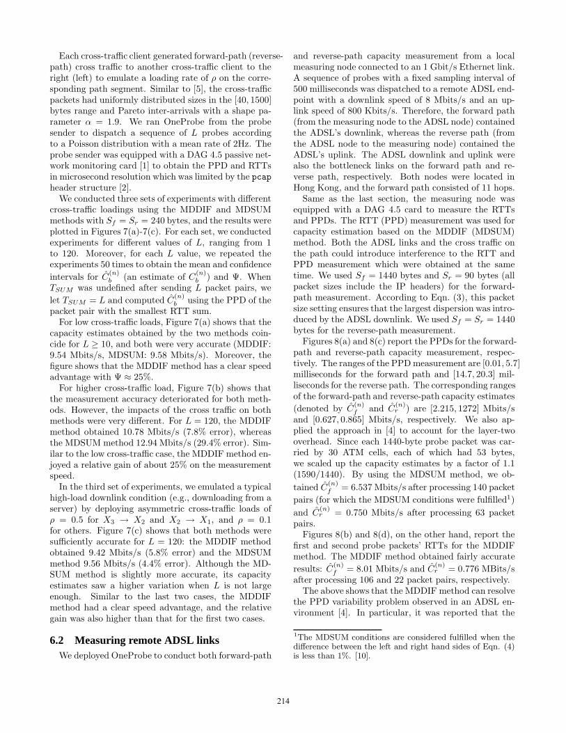
We conducted three sets of experiments with differentcross-traffic loadings using the MDDIF and MDSUMmethods with Sf = Sr = 240 bytes, and the results wereplotted in Figures 7(a)-7(c). For each set, we conductedexperiments for different values of L, ranging from 1to 120. Moreover, for each L value, we repeated theexperiments 50 times to obtain the mean and confidence

intervals for C(n)b (an estimate of C

(n)b ) and Ψ. When

TSUM was undefined after sending L packet pairs, we

let TSUM = L and computed C(n)b using the PPD of the

packet pair with the smallest RTT sum.For low cross-traffic loads, Figure 7(a) shows that the

capacity estimates obtained by the two methods coin-cide for L ≥ 10, and both were very accurate (MDDIF:9.54 Mbits/s, MDSUM: 9.58 Mbits/s). Moreover, thefigure shows that the MDDIF method has a clear speedadvantage with Ψ ≈ 25%.

For higher cross-traffic load, Figure 7(b) shows thatthe measurement accuracy deteriorated for both meth-ods. However, the impacts of the cross traffic on bothmethods were very different. For L = 120, the MDDIFmethod obtained 10.78 Mbits/s (7.8% error), whereasthe MDSUM method 12.94 Mbits/s (29.4% error). Sim-ilar to the low cross-traffic case, the MDDIF method en-joyed a relative gain of about 25% on the measurementspeed.

In the third set of experiments, we emulated a typicalhigh-load downlink condition (e.g., downloading from aserver) by deploying asymmetric cross-traffic loads ofρ = 0.5 for X3 → X2 and X2 → X1, and ρ = 0.1for others. Figure 7(c) shows that both methods weresufficiently accurate for L = 120: the MDDIF methodobtained 9.42 Mbits/s (5.8% error) and the MDSUMmethod 9.56 Mbits/s (4.4% error). Although the MD-SUM method is slightly more accurate, its capacityestimates saw a higher variation when L is not largeenough. Similar to the last two cases, the MDDIFmethod had a clear speed advantage, and the relativegain was also higher than that for the first two cases.

6.2 Measuring remote ADSL linksWe deployed OneProbe to conduct both forward-path

and reverse-path capacity measurement from a localmeasuring node connected to an 1 Gbit/s Ethernet link.A sequence of probes with a fixed sampling interval of500 milliseconds was dispatched to a remote ADSL end-point with a downlink speed of 8 Mbits/s and an up-link speed of 800 Kbits/s. Therefore, the forward path(from the measuring node to the ADSL node) containedthe ADSL’s downlink, whereas the reverse path (fromthe ADSL node to the measuring node) contained theADSL’s uplink. The ADSL downlink and uplink werealso the bottleneck links on the forward path and re-verse path, respectively. Both nodes were located inHong Kong, and the forward path consisted of 11 hops.

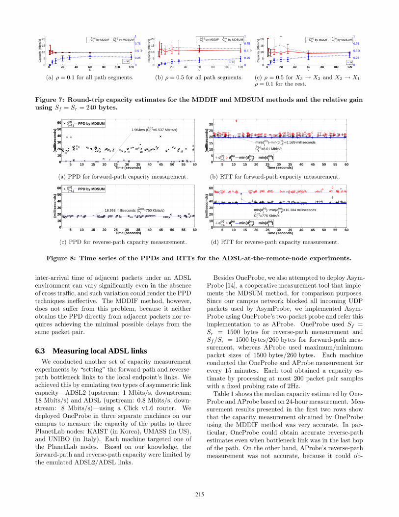
Same as the last section, the measuring node wasequipped with a DAG 4.5 card to measure the RTTsand PPDs. The RTT (PPD) measurement was used forcapacity estimation based on the MDDIF (MDSUM)method. Both the ADSL links and the cross traffic onthe path could introduce interference to the RTT andPPD measurement which were obtained at the sametime. We used Sf = 1440 bytes and Sr = 90 bytes (allpacket sizes include the IP headers) for the forward-path measurement. According to Eqn. (3), this packetsize setting ensures that the largest dispersion was intro-duced by the ADSL downlink. We used Sf = Sr = 1440bytes for the reverse-path measurement.

Figures 8(a) and 8(c) report the PPDs for the forward-path and reverse-path capacity measurement, respec-tively. The ranges of the PPD measurement are [0.01, 5.7]milliseconds for the forward path and [14.7, 20.3] mil-liseconds for the reverse path. The corresponding rangesof the forward-path and reverse-path capacity estimates

(denoted by C(n)f and C

(n)r ) are [2.215, 1272] Mbits/s

and [0.627, 0.865] Mbits/s, respectively. We also ap-plied the approach in [4] to account for the layer-twooverhead. Since each 1440-byte probe packet was car-ried by 30 ATM cells, each of which had 53 bytes,we scaled up the capacity estimates by a factor of 1.1(1590/1440). By using the MDSUM method, we ob-

tained C(n)f = 6.537 Mbits/s after processing 140 packet

pairs (for which the MDSUM conditions were fulfilled1)

and C(n)r = 0.750 Mbits/s after processing 63 packet

pairs.Figures 8(b) and 8(d), on the other hand, report the

first and second probe packets’ RTTs for the MDDIFmethod. The MDDIF method obtained fairly accurate

results: C(n)f = 8.01 Mbits/s and C

(n)r = 0.776 MBits/s

after processing 106 and 22 packet pairs, respectively.The above shows that the MDDIF method can resolve

the PPD variability problem observed in an ADSL en-vironment [4]. In particular, it was reported that the

1The MDSUM conditions are considered fulfilled when thedifference between the left and right hand sides of Eqn. (4)is less than 1%. [10].

214

0 20 40 60 80 100 1200

5

10

15

20

L

Cap

acity

(M

bits

/s)

0 20 40 60 80 100 1200

0.25

0.5

0.75

1

Ψ

C(n)b

by MDDIF C(n)b

by MDSUM

Ψ

^ ^

(a) ρ = 0.1 for all path segments.

0 20 40 60 80 100 1200

5

10

15

20

L

Cap

acity

(M

bits

/s)

0

0.25

0.5

0.75

1

Ψ

C(n)b

by MDDIF C(n)b

by MDSUM

Ψ

^^

(b) ρ = 0.5 for all path segments.

0 20 40 60 80 100 1200

5

10

15

20

Cap

acity

(M

bits

/s)

0 20 40 60 80 100 1200

0.25

0.5

0.75

1

L

Ψ

C(n)b

by MDDIF C(n)b

by MDSUM

Ψ

^^

(c) ρ = 0.5 for X3 → X2 and X2 → X1;ρ = 0.1 for the rest.

Figure 7: Round-trip capacity estimates for the MDDIF and MDSUM methods and the relative gainusing Sf = Sr = 240 bytes.

5 10 15 20 25 30 35 40 45 50 55 600

10

20

30

40

50

60

Time (seconds)

(mill

isec

onds

)

δ(n)j−1,j PPD by MDSUM

1.964ms (C(n)f

=6.537 Mbits/s)^

(a) PPD for forward-path capacity measurement.

5 10 15 20 25 30 35 40 45 50 55 600

5

10

15

20

25

30

Time (seconds)

(mill

isec

onds

)

d(n)j−1

d(n)j

min{d (n)j−1

} min{d (n)j

}

C(n)f

=8.01 Mbits/s^min{d(n)

j}−min{d(n)

j−1}=1.589 milliseconds

(b) RTT for forward-path capacity measurement.

5 10 15 20 25 30 35 40 45 50 55 600

10

20

30

40

50

60

Time (seconds)

(mill

isec

onds

)

δ(n)j−1,j PPD by MDSUM

16.968 milliseconds (C(n)r

=750 Kbits/s)^

(c) PPD for reverse-path capacity measurement.

5 10 15 20 25 30 35 40 45 50 55 600

10

20

30

40

50

60

Time (seconds)

(mill

isec

onds

)

d(n)j−1

d(n)j

min{d (n)j−1

} min{d (n)j

}

C(n)r

=776 Kbits/s^min{d(n)

j}−min{d(n)

j−1}=16.384 milliseconds

(d) RTT for reverse-path capacity measurement.

Figure 8: Time series of the PPDs and RTTs for the ADSL-at-the-remote-node experiments.

inter-arrival time of adjacent packets under an ADSLenvironment can vary significantly even in the absenceof cross traffic, and such variation could render the PPDtechniques ineffective. The MDDIF method, however,does not suffer from this problem, because it neitherobtains the PPD directly from adjacent packets nor re-quires achieving the minimal possible delays from thesame packet pair.

6.3 Measuring local ADSL linksWe conducted another set of capacity measurement

experiments by “setting” the forward-path and reverse-path bottleneck links to the local endpoint’s links. Weachieved this by emulating two types of asymmetric linkcapacity—ADSL2 (upstream: 1 Mbits/s, downstream:18 Mbits/s) and ADSL (upstream: 0.8 Mbits/s, down-stream: 8 Mbits/s)—using a Click v1.6 router. Wedeployed OneProbe in three separate machines on ourcampus to measure the capacity of the paths to threePlanetLab nodes: KAIST (in Korea), UMASS (in US),and UNIBO (in Italy). Each machine targeted one ofthe PlanetLab nodes. Based on our knowledge, theforward-path and reverse-path capacity were limited bythe emulated ADSL2/ADSL links.

Besides OneProbe, we also attempted to deploy Asym-Probe [14], a cooperative measurement tool that imple-ments the MDSUM method, for comparison purposes.Since our campus network blocked all incoming UDPpackets used by AsymProbe, we implemented Asym-Probe using OneProbe’s two-packet probe and refer thisimplementation to as AProbe. OneProbe used Sf =Sr = 1500 bytes for reverse-path measurement andSf/Sr = 1500 bytes/260 bytes for forward-path mea-surement, whereas AProbe used maximum/minimumpacket sizes of 1500 bytes/260 bytes. Each machineconducted the OneProbe and AProbe measurement forevery 15 minutes. Each tool obtained a capacity es-timate by processing at most 200 packet pair sampleswith a fixed probing rate of 2Hz.

Table 1 shows the median capacity estimated by One-Probe and AProbe based on 24-hour measurement. Mea-surement results presented in the first two rows showthat the capacity measurement obtained by OneProbeusing the MDDIF method was very accurate. In par-ticular, OneProbe could obtain accurate reverse-pathestimates even when bottleneck link was in the last hopof the path. On the other hand, AProbe’s reverse-pathmeasurement was not accurate, because it could ob-

215

tain only the forward-path dispersion and therefore theestimates represent the lower bounds for the reverse-path capacity. Nonetheless, AProbe still obtained lowerbound values for the two ADSL cases: 1500/260×0.8 =4.615 Mbits/s and 1500/260× 1 = 5.769 Mbits/s.

We repeated the experiments with a symmetric net-work link of 10 Mbits/s which, according to the reasonsstated earlier, should be the bottleneck capacity. Allother settings were unchanged. As shown in the thirdrow of Table 1, OneProbe’s and AProbe’s results wereclose to 10 Mbits/s. We did not try a higher bandwidth,because we were no longer able to ensure that the bot-tleneck link was still located in our campus network.

Table 1: Median capacity (in Mbits/s) measuredby OneProbe and AProbe.

Link Tools KAIST UMASS UNIBO

Type C(n)f

C(n)r C

(n)f

C(n)r C

(n)f

C(n)r

ADSL OneProbe 0.799 7.921 0.771 7.926 0.798 7.900(Up = 0.8, AProbe 0.786 4.392 0.758 4.544 0.758 4.310Down = 8)

ADSL2 OneProbe 1.018 17.817 0.962 17.870 0.991 17.804(Up = 1, AProbe 0.988 5.472 0.989 5.262 1.025 5.300

Down = 18)

10 Mbits/s OneProbe 10.025 9.748 10.568 9.748 10.353 9.744Ethernet AProbe 10.592 9.740 9.423 9.748 9.630 9.748

Link

7. CONCLUSIONSThis paper introduced the minimum delay difference

(MDDIF) method, a new cross-traffic filtering approachfor capacity measurement. Unlike the existing packet-pair dispersion methods, the MDDIF method obtainsthe packet-pair dispersion from the minimal possibledelay (minDelay) for a first probe packet and a secondprobe packet both of which generally belong to differ-ent packet pairs. We have proved that a difference ofthese two minDelays gives the packet-pair dispersionrequired for capacity estimation and that the MDDIFmethod is faster than the minimum delay sum (MD-SUM) method. We also conducted testbed and Internetmeasurement experiments to compare the MDDIF andMDSUM methods.

AcknowledgmentsWe thank the four anonymous reviewers for their criti-cal reviews and suggestions and Paolo Giaccone, in par-ticular, for shepherding our paper. This work is par-tially supported by a grant (ref. no. ITS/152/08) fromthe Innovation Technology Fund and a grant (ref. no.H-ZL17) from the Joint Universities Computer Centre,both in Hong Kong.

8. REFERENCES[1] endace. http://www.endace.com/.[2] TCPDUMP/LIBPCAP public repository.

http://www.tcpdump.org/.[3] J. Bolot. End-to-end packet delay and loss behavior in

the Internet. In Proc. ACM SIGCOMM, 1993.[4] D. Croce, T. En-Najjary, G. Urvoy-Keller, and

E. Biersack. Capacity estimation of ADSL links. InProc. ACM CoNEXT, 2008.

[5] C. Dovrolis, P. Ramanathan, and D. Moore. Packetdispersion techniques and a capacity-estimationmethodology. IEEE/ACM Trans. Netw., 12(6), 2004.

[6] A. Downey. Using pathchar to estimate Internet linkcharacteristics. In Proc. ACM SIGCOMM, 1999.

[7] K. Harfoush, A. Bestavros, and J. Byers. Measuringcapacity bandwidth of targeted path segments.IEEE/ACM Trans. Netw., 17(1), 2009.

[8] S. Hemminger. Network emulation with NetEm. Inlinux.conf.au, 2005.

[9] V. Jacobson. Pathchar: A tool to infer characteristicsof Internet paths. ftp://ftp.ee.lbl.ogv/pathchar/.

[10] R. Kapoor, L. Chen, L. Lao, M. Gerla, andM. Sanadidi. CapProbe: A simple and accuratecapacity estimation technique. In Proc. ACMSIGCOMM, 2004.

[11] T. Karagiannis, M. Molle, M. Faloutsos, andA. Broido. A nonstationary Poisson view of Internettraffic. In Proc. IEEE INFOCOM, 2004.

[12] J. Kemeny and J. Snell. Finite Markov Chains.Springer, 1976.

[13] L. Kleinrock. Queueing Systems, Vol. 2: ComputerApplications. Wiley-Interscience, 1976.

[14] L. Chen, T. Sun, G. Yang, M. Sanadidi, and M. Gerla.End-to-end asymmetric link capacity estimation. InProc. IFIP Networking, 2005.

[15] K. Lai and M. Baker. Measuring bandwidth. In Proc.IEEE INFOCOM, 1999.

[16] K. Lai and M. Baker. Measuring link bandwidthsusing a deterministic model of packet delay. Proc.ACM SIGCOMM, 2000.

[17] X. Luo, E. Chan, and R. Chang. Design andimplementation of TCP data probes for reliable andmetric-rich network path monitoring. In Proc.USENIX Annual Tech. Conf., 2009.

[18] B. Mah. pchar: A tool for measuring Internet pathcharacteristics.http://www.kitchenlab.org/bmah/Software/pchar/.

[19] J. Mogul. Observing TCP dynamics in real networks.In Proc. ACM SIGCOMM, 1992.

[20] R. Nelson. Probability, Stochastic Processes, andQueueing Theory: The Mathematics of ComputerPerformance Modelling. Springer, 1995.

[21] L. Nussbaum and O. Richard. A comparative study ofnetwork link emulators. In Proc. CNS, 2009.

[22] A. Pasztor and D. Veitch. The packet size dependenceof packet-pair like methods. In Proc. IWQoS, 2002.

[23] V. Paxson. Measurements and Analysis of End-to-EndInternet Dynamics. PhD dissertation, University ofCalifornia Berkeley, 1997.

[24] R. Carter and M. Crovella. Measuring bottleneck linkspeed in packet-switched networks. PerformanceEvaluation, 1996.

[25] S. Saroiu, P. Gummadi, and S. Gribble. Sprobe: Afast technique for measuring bottleneck bandwidth inuncooperative environments. In Proc. IEEEINFOCOM, 2002.

216