Embed Size (px)
Citation preview

Proximal Policy Optimization via EnhancedExploration Efficiency
Junwei Zhanga,b, Zhenghao Zhanga,b, Shuai Hana,b, Shuai Lua,b,∗
aKey Laboratory of Symbolic Computation and Knowledge Engineering (Jilin University),Ministry of Education, Changchun 130012, China
bCollege of Computer Science and Technology, Jilin University, Changchun 130012, China
Abstract
Proximal policy optimization (PPO) algorithm is a deep reinforcement learn-
ing algorithm with outstanding performance, especially in continuous control
tasks. But the performance of this method is still affected by its exploration
ability. For classical reinforcement learning, there are some schemes that make
exploration more full and balanced with data exploitation, but they can’t be
applied in complex environments due to the complexity of algorithm. Based on
continuous control tasks with dense reward, this paper analyzes the assumption
of the original Gaussian action exploration mechanism in PPO algorithm, and
clarifies the influence of exploration ability on performance. Afterward, aiming
at the problem of exploration, an exploration enhancement mechanism based
on uncertainty estimation is designed in this paper. Then, we apply exploration
enhancement theory to PPO algorithm and propose the proximal policy op-
timization algorithm with intrinsic exploration module (IEM-PPO) which can
be used in complex environments. In the experimental parts, we evaluate our
method on multiple tasks of MuJoCo physical simulator, and compare IEM-
PPO algorithm with curiosity driven exploration algorithm (ICM-PPO) and
original algorithm (PPO). The experimental results demonstrate that IEM-PPO
algorithm needs longer training time, but performs better in terms of sample
efficiency and cumulative reward, and has stability and robustness.
∗Corresponding authorEmail address: [email protected] (Shuai Lu)
Preprint submitted to Information Sciences November 12, 2020
arX
iv:2
011.
0552
5v1
[cs
.LG
] 1
1 N
ov 2
020
Keywords: deep reinforcement learning, continuous control tasks, exploration
enhancement, uncertainty estimation, proximal policy optimization algorithm
1. Introduction
Deep reinforcement learning combines the efficient representation and per-
ception ability in deep learning with the decision-making ability in reinforcement
learning, which can learn and optimize the policies via interacting with complex
environments. This approach, which is closer to the human mode of thinking,
has achieved remarkable results in arcade games [1, 2], physical simulation en-
vironments [3, 4] and real tasks [5, 6], but is also facing with more complex
modeling and training processes.
In the application of reinforcement learning algorithm, the environment data
should be processed according to actual situation. According to action charac-
teristics, simulation environment tasks can be divided into discrete action tasks
and continuous action tasks. Although both two action types can be generated
by corresponding neural networks [7, 8], the outputs and the performance will
be greatly different due to different model architectures.
In continuous action tasks, proximal policy optimization algorithm [9] pro-
posed by Schulman in 2017 performs well. It has the advantages of stable
training process, high performance and scalability. However, some researchers
also find it difficult to reproduce PPO algorithm, which mainly due to the sen-
sitivity of hyperparameters, and agent could not balance the exploration of the
environment and the exploitation of data [10], so that the agent’s policy easily
falls into local optima.
The Gaussian action exploration mechanism in PPO samples actions from
a Gaussian distribution, which adds a certain range of variance as the noise to
the output of policy network. Such an exploration mechanism samples actions
with equal probability in opposite directions from the current mean, which can
stably optimize the policy towards the optimal decision direction theoretically.
However, due to the limited number of interactions with the environment and
2
the estimation error [11], this mechanism tends to fall into the local optima. We
will illustrate the relationship between the exploration scope and the suboptimal
solution by experiments with different exploration settings.
In physical simulation environment, we construct deep neural network to
estimate the uncertainty of action. And the uncertain value of observation state
is used to stimulate action selection, so as to encourage the action to explore
in the direction of great uncertainty and avoid converging prematurely to local
optima. Our approach also provides a trend for agent to explore further. This
mechanism is applied to PPO algorithm, and we call it IEM-PPO (proximal
policy optimization with intrinsic exploration module).
In the experiment, we use MuJoCo tasks, which have been widely recognized
in recent years. While reproducing PPO algorithm, we optimize and adjust the
algorithm settings according to the experimental environment. The expected
results are achieved in all tasks, and in some tasks are better than those given in
PPO literature [9]. We apply curiosity driven mechanism [12] to PPO algorithm
for the comparative experiment. The experiment demonstrates that although
the exploration enhancement algorithm proposed in this paper requires longer
training time, it performs better in terms of sample efficiency and cumulative
reward, and has stronger stability and robustness.
Our main contributions are as follows: 1) We analyze the defect of Gaussian
noise exploration and show that exploration enhancement mechanism can play
a certain role in dense reward continuous tasks. 2) Based on the uncertainty
theory, an effective mechanism of exploration enhancement is proposed. On
Mujoco benchmarks, our algorithm outperforms previous algorithms and more
stable.
2. Related Work
At present, most practical deep reinforcement learning methods still rely on
simple exploration rules, such as ε-greedy in DQN [13], Gaussian noise in DDPG
[14] and PPO, and entropy regularization in A3C [15] to prevent premature
3

convergence in the early stage of training. This kind of methods hardly introduce
deviation in the optimization process, but low efficiency, especially in continuous
action tasks, easy to fall into the local optima.
For exploration and exploitation, Pathak et al. introduce curiosity driven
mechanism into Actor-Critic framework of deep reinforcement learning in view
of the most complex environments in Atari [12]. They define curiosity as the
error in the perception of environmental changes, and combine such error as
internal incentive with external reward of environment as the training data.
Their algorithm performs well in the discrete tasks with sparse reward [16].
However, it is difficult to predict environmental change which is influenced by
bias and noise. The performance is limited when curiosity driven algorithm is
applied to continuous tasks with dense reward, such as MuJoCo. Performance
comparison can be seen in our experiment section.
In reinforcement learning with table method, it has been found that the
uncertainty of observation state is negatively correlated with the number of
states visited. Therefore, Auer et al. [17] and Stehl et al. [18] respectively
propose the theory of exploration enhancement based on uncertainty in 2002
and 2008, which could theoretically fully explore the environment and maintain
consistency of the optimal policy. However, after the combination of deep learn-
ing and reinforcement learning, some exploration mechanism cannot be used in
complex tasks due to the time and space complexity.
In addition, in DQN, noise can be added to the parameter space of the
neural network to assist the exploration [19]. However, in PPO and other policy
gradient algorithms, the current policy is directly optimized without maintaining
global Q function, so it’s difficult to apply the noise in the parameter space.
3. Background
Reinforcement learning, as one of the important branches of machine learn-
ing, is mainly aimed at decision-making and optimization problems. Without
accurate label data, the optimal policies can be obtained by trial and error
4

through interaction with the environment.
3.1. Problem description
In order to solve reinforcement learning problem, it is usually modeled as
Markov decision process (MDP). MDP is a mathematical model to deal with
sequential decision making problem, which is applied to simulate the stochastic
policies and rewards of an agent in an environment with Markov property. MDP
is usually abstracted as a tuple representation < S,A, P,R, γ >, where:
• S is a set of all states in the environment;
• A is a set of executable actions of the agent;
• P is a transition distribution, P ass′
= P(St+1 = s
′∣∣∣St = s,At = a
);
• R is a return function, and Rt represents the environmental return ob-
tained after taking an action at time t;
• γ is a discount factor, which is used to calculate the cumulative reward,
where γ ∈ [0, 1].
Agent selects an action to execute by action selection policy which we need
to optimize. The policy is a probability distribution of actions under given
state, represented by π (a|s), where π (a|s) = P (At = a|St = s). That is the
probability of agent chooses action a under the current state s at time t.
The goal of reinforcement learning is to maximize the reward value, which is
usually calculated by using cumulative reward function Gt, defined as formula
(1).
Gt = Rt + γRt+1 + γ2Rt+2 + . . . =
∞∑k=0
γkRt+k (1)
where, the discount factor γ is added to adjust the weighting between immediate
and delayed outcomes. The greater discount factor is, the more focus agent puts
on delayed outcomes. Cumulative reward function Gt has become one of the
criteria to evaluate policy in MDP problems [4, 9, 15].
5

3.2. Policy gradient
The policy gradient as a way to find optimal policy, samples environment
interaction of agent and calculates the gradient of current policy directly, then
optimizes the current stochastic policy [20].
In the policy gradient algorithm, the process from the starting to the termi-
nation of the task is called an episode τ , where τ = {s1, a1, s2, a2, . . . , sT , aT }.
We need to maximize the cumulative reward function for all episodes. Therefore,
the optimal policy is shown in formula (2).
π∗ = argmaxπEτ∼π(τ) [R (τ)] (2)
Therefore, the policy value is shown in formula (3).
L (θ) = Eτ∼πθ(τ) [R (τ)] =∑
τ∼πθ(τ)
Pθ (τ)R (τ) (3)
where, θ is the current model parameter, Pθ (τ) =T∏t=1
πθ (at|st)P (at+1|st, at)
is occurrence probability of current trajectory. Since environment transition
distribution is independent of model parameters, P (at+1|st, at) is not consid-
ered. After calculating the gradient of the objective function L (θ), formula (4)
is shown as following:
∇θL (θ) ≈∑
τ∼πθ(τ)
R (τ)∇θlogπθ (τ) ≈ 1
N
N∑n=1
T∑t=1
R (τn)∇θlogπθ (ant |snt ) (4)
Therefore, policy gradient algorithm is divided into following two steps for
continuous iterative update:
1) Use πθ to interact with environment, and obtain the observed data and
calculate ∇θL (θ).
2) Update θ with gradient and learning rate α, where θ = θ + α∇θL (θ).
6

3.3. Deep learning and variance control
In the complex environment, due to time and space complexity of algorithm,
it is no longer possible to maintain the value table of each state-action pair.
Therefore, it is necessary that agent utilizes powerful representation ability of
neural network to calculate the value function and make decision [21].
In the simple environment, an accurate estimation of policy gradient can be
achieved with a small number N of sampled trajectories. Due to the increase of
environment complexity, the demand for the number of sample trajectories also
increase. In order to ensure the performance in tasks, N is hard to get enough.
In order to solve the problem of variance increase due to insufficient sampling
[22], the strategy of variance reduction is usually used to ensure the accuracy
of gradient estimation. This variance reduction strategy is based on such two
ideas:
1) The action at current moment t has nothing to do with reward at the
past moment t′. At t > t
′, there is E
[∇θπθ (at|st)R
′
t
]= 0.
2) Adding or subtracting constant V (st) to current state value Rt will
not introduce bias into policy gradient, and variance can be reduced, that is
E [∇θπθ (at|st)V (st)] = 0. Therefore, At =T∑t′=t
(Rt′ − V (st)) is used to replace
R (τn) in the calculation of policy gradient.
Thus, the more accurate optimization objective function is shown in formula
(5).
∇θL (θ) =1
N
N∑n=1
T∑t=1
Ant∇θlogπθ (ant |snt ) (5)
where, At is called advantage value, representing the difference between the
value of action taken and the average value in the current state. In training
process, average value of current state cannot be calculated, but can be fitted
by using supervised learning based on deep neural network. Therefore, two
neural network approximators are needed to calculate the policy gradient in
training. One is to compute πθ, which is used to select actions, the other is
7

to compute V (st) , which gives average value of current state and is used to
calculate At.
3.4. Proximal policy optimization algorithm
The policy gradient algorithm is implemented by calculating estimated value
of policy gradient and using stochastic gradient ascent optimization. Formula
(6) is taken as the form of policy estimation:
∇θL (θ) = Et
[∇θlogπθ (at|st)At
](6)
where, πθ is stochastic policy, At is estimation of advantage value. Expected
value Et is calculated by averaging the set of sampling values. The algorithm
continuously alternates in sampling and optimization. This estimation ∇θL (θ)
is the derivative of objective function (7).
LPG (θ) = Et
[logπθ (at|st)At
](7)
In order to improve training efficiency and make sampled data reusable [9],
πθ (at|st) /πθold (at|st) is used instead of logπθ (at|st) to support off-policy train-
ing. However, in this way, the difference between new and old policies should not
be too large. Otherwise, many samples are needed to get the correct estimation
due to the increase of variance.
It can be seen from objective function that: when At > 0 , the policy will
optimize in the direction that logπθ (at|st) increases, thence the probability of
selecting the current action at will increase. The size of training step is deter-
mined by the combination of action selection probability π, advantage function
A and learning rate α. If the learning rate is limited to a small range to en-
sure policy changes little, the probability of policy falling into local optima will
increase.
In PPO algorithm, a clipping mechanism is added to objective function to
punish the policy change, when πθ (at|st) /πθold (at|st) is away from 1, which
represents policy updating generated by the maximized objective function is
8

excessive. Final objective function is shown in formula (8).
LCLIP (θ) = Et
[min
(rt (θ) At, clip (ε, rt (θ)) At
)](8)
where, rt (θ) = πθ (at|st) /πθold (at|st) represents action selection probability ra-
tio of new and old policies. In the min operation, the first item is the original
optimization goal, and the second item is clip function which modifies the sur-
rogate objective by clipping the probability ratio. The clip function removes
the incentive for moving rt outside of the interval [1− ε, 1 + ε], where ε is hy-
perparameter. In this scheme, only large changes in the direction of policy
improvement are removed, while in the policy decline are retained. According
to the comparing results of the Mujoco experiments [9], ε is set to 0.2. The per-
formance is less affected by ε values. The PPO algorithm is shown in Algorithm
1.
Algorithm 1 PPO
1: Initial policy parameters θ0 and value function parameters φ0.2: for k = 0,1,2, . . . do3: Collect set of trajectories Dk = {τi} by running policy πk = π (θk) in the
environment.4: Compute reward-to-go Rt.5: Compute advantage estimation At based on value function Vφ.6: Update the policy with Adam by maximizing the clip objective:
θk+1 = arg maxθ
1|Dk|T
∑τ∈Dk
T∑t=0
min(πθ(at|st)πθk (at|st)
At, clip (ε, rt (θ)) At
).
7: Approximate value function via gradient descent algorithm by regressionon mean-squared error:
φk+1 = arg minφ
1|Dk|T
∑τ∈Dk
T∑t=0
(Rt − Vφ (st)
)2.
8: end for
9

4. Enhance exploration ability
In discrete action tasks with sparse reward, the relative insufficiency of ex-
ploration ability can be obviously detected. However, for continuous action
tasks with dense reward, the problem of balancing between exploration and ex-
ploitation still exists. Original exploration mechanism may not enough to make
exploration and exploitation reach a balanced situation.
4.1. Exploration and exploitation of continuous action tasks
In reinforcement learning environments, policy optimization needs to max-
imize cumulative reward. For any state s, depending on the number of state
visits, the degree of perception of alternative actions is usually different. Even
when the policy reward reach convergence, there are also unselected or less se-
lected actions, and the evaluation of such actions is often inaccurate. In training
process, exploitation is to use the current policy in order to obtain better reward
value with current perception; exploration is trying different actions to gather
more information. A good long-term training usually needs sacrifice short-term
gains by gathering enough information to enable an agent to get a global optimal
solution. Although exploration and exploitation are contradictory processes, a
good exploration strategy can improve performance and an efficient exploitation
strategy can also increase the scope of exploration.
When using PPO algorithm to solve continuous action tasks, the policy
network selects an appropriate action µt according to the acquired knowledge.
In order to explore unknown actions, Gaussian noise N (0, σ) is added to action
µt to obtain at, as shown in formula (9). The at is used as the final action to
interact with environment.
at = µt +N (0, σ) (9)
Therefore, this kind of action selection with noise is classified as a stochastic
policy in continuous action space. According to mathematical characteristics of
Gaussian distribution, formula (10) can be used to obtain likelihood probability
10

of taking current action at:
logP (at) =
n∑i=1
−1
2
((ati − µti
σi
)2
+ 2logσi + log2π
)(10)
The value of σ in Gaussian noise will determine the ability to select unknown
actions in current policy. The larger σ tends to select unknown actions, which
will lead to problems of low training efficiency and policy instability, while stable
policy get higher scores in most tasks. If a smaller σ value is chosen, exploration
ability is poor, the policy would fall into local optima. Therefore, σ should be
selected as hyperparameter of a certain problem.
According to optimization theory: In initial stage of neural network approx-
imating optimization, giving a large learning rate of parameters, the algorithm
can have a stronger ability to jump out of local optima. It tends to choose a
more appropriate optimization point in global. As the learning process contin-
ues to reduce learning rate, the ability to approximate optimal value becomes
stronger. PPO algorithm could use a dynamic σ setting, cumulative reward
is used as the index to measure learning progress. Exploration scope decreases
with the increase of cumulative reward, which has a better training effect. Since
cumulative reward values of the task within a fixed range, training effects are
still different for different initial values. If inappropriate exploration parameters
are given, the whole experiment process will be affected.
We use experiments to verify the theory. The experimental environment is
Halfcheetah-v2 in MuJoCo. Details of the environment will be introduced in
the experimental section. The experimental results of fixed σ and dynamic σ
settings based on cumulative reward are shown in Figure 1.
In Figure 1, training results of four fixed exploration value settings {0.6,
0.4, 0.2, 0.1} and training results of six dynamic σ settings under different
initial values of training {0.8, 0.7, 0.6, 0.5, 0.4, 0.2} are respectively shown.
The abscissa represents the number of interactions with the environment, the
ordinate represents the sum of reward of each episode. It can be seen from the
experimental results that the final performance set by dynamic σ can converge to
11

Figure 1: Experiments of various fixed σ settings (left) and dynamic σ value settings (right)in Halfcheetah-v2 environment
5000, which is better than the fixed σ settings of 4000. And in different settings,
the problem of falling into local optimum is common. For the Halfcheetah-v2
task, the dynamic σ setting with the initial value of 0.6 is better, all other
settings present some degree of local optimum problem.
4.2. Curiosity driven mechanism
In some tasks, for example, Montezuma’s revenge in Atari 2600, there are
situations where external reward available to agent is sparse. However, for
reinforcement learning tasks, an agent constantly explores environment until it
gets a reward, and then can improve the policy so that it can get better reward
and learn policies in future. Hoping to get a reward by chance (i.e. random
exploration) is likely to be futile for all but the simplest of environments [12].
In curiosity theory, internal incentive signals add to the original environ-
mental reward, and it uses existing data information to expand the original
sparse reward for reasonable reward form dense, which assists agent with better
exploration. Formally expressed as formula (11).
Rt = Rit +Ret (11)
The addition of internal incentive signals are intended to stimulate the di-
rection to novel states, which increases the probability of revisiting and further
12

exploration in this direction during policy learning. Therefore, internal incen-
tive signals mainly determine the specification for whether a state is novel in a
complex environment. At modeling, measuring “novelty” requires a statistical
model of the distribution of environmental states, that is, getting how novel of
the current state after giving certain observations.
In curiosity module, curiosity is defined as the error of predicting the result of
one’s own behavior, in other words, the perception of agent on the degree of the
environment affected by current actions. In modeling, the forward prediction
model is joined, current state and action as neural network input. We use the
multilayer neural network, output next state observation values and minimize
mean square error (MSE) as training target. Prediction model gets internal
incentive signals and trains positive ability to predict observation state. The
mixed reward is shown in formula (12).
Rt = Rit + β ‖fψ (st, at)− st+1‖22 (12)
where, fψ (st, at) is forward neural network with parameter ψ, β is hyperparam-
eter which serves as the balance ratio between internal incentive and external
reward, which needs experimental adjustments to eliminate dimensional influ-
ence.
Previously, the curiosity module is mainly aimed at tasks with insufficient
external reward signals, but theoretically, these internal incentive signals give
a new direction of exploration in the short term. In continuous action tasks,
the introduction of curiosity module points to a new mechanism for enhancing
exploration. Different from original Gaussian noise, internal incentive can en-
courage the exploration of novel states for a short time. If internal incentive and
Gaussian random action can act together, directional exploration enhancement
can be guaranteed under the condition of less action noise.
In order to demonstrate the performance of curiosity module, we use Halfcheetah-
v2 in MuJoCo to carry out experimental test. Experimental results are shown
in Figure 2.
13

Figure 2: Comparison experiment of curiosity driven algorithm (ICM-PPO) and PPO algo-rithm in Halfcheetah-v2 environment
In Figure 2, curiosity driven algorithm and PPO algorithm run three times
respectively. The results are averaged and the variance is marked with shadows.
It can be seen that after the introduction of curiosity module, training speed
in the early stage has little impact, but in the middle and late stages, due to
the full perceptive learning of state which fewer visit in original algorithm, it
achieves a higher cumulative reward. Although improvement is small, it can
be explained that curiosity driven module, as a directional guide to exploration
mechanism, has certain effects on continuous action tasks and can play a role
in enhancing training efficiency. Curiosity algorithm is taken as one of the
experimental comparison algorithms in this paper, more complete experiments
and analyses will be given in the experiment section.
4.3. Exploration enhancement based on uncertainty estimation
Just as previous analysis of PPO algorithm, original Gaussian noise explo-
ration has fallen into a dilemma, which is mainly summarized as the following
two points:
(1) Gaussian exploration is sensitive to hyperparameters.
The performance is seriously affected by the initial value in both fixed and
dynamically adjusted σ. Moreover, when initial values are small, it is easy to
fall into the local optima; when initial values are large, the exploration scope
14
is increased, and the policy will be unstable which ultimately is difficult to
converge.
(2) Exploration efficiency is insufficient.
In the process of action selection, Gaussian noise exploration mechanism
samples actions with equal probability in opposite directions from the current
mean. In order to ensure exploration ability, initial exploration scope must be
set as a large value. Some actions are no longer necessary for further exploration,
repeating exploration slows down learning efficiency.
Therefore, for continuous action tasks, a directional exploration mechanism
that can be used for low-Gaussian noise action selection will improve explo-
ration ability of the algorithm. We design an enhanced exploration algorithm
by analyzing exploration mechanism of table method.
Prior to the rise of deep learning and its integration with reinforcement
learning, reinforcement learning used tabular methods to record updates and
iterations of state and action value. Although deep reinforcement learning per-
forms well in various tasks, most of mechanisms in the original reinforcement
learning cannot be transferred into deep reinforcement learning due to the lim-
itations of data processing, such as uncertain behavior exploration.
Uncertain behavior exploration method relis on the concept of information
entropy. Action reward is represented by distribution function. If the variance of
distribution function is large, then it contains more information; if the variance
of action reward distribution is small, it requires fewer visits to determine actual
action reward. Therefore, in order to obtain the maximum exploration ability,
action reward distribution with large variance should be explored first.
Since uncertain behavior exploration always gives priority to exploration of
actions with great uncertainty, it is also called optimistic exploration. There
is relatively great uncertainty in the states with few visits. It is potentially
believed that there is a better policy scheme in unknown actions. The bonus of
the state s is added based on the number of visits N(s), as shown in formula
15
(13).
r+ (s, a) = r(s, a) +B(N(s)) (13)
In 2008, Stehl et al. [18] consider the impact of interaction times on the
uncertainty. On the basis of improving the exploration efficiency, algorithm
ensures the environment with no bias of optimal policy and is more convenient
to calculate, as shown in formula (14).
B(N(s)) =
√1
N(s)(14)
As the training progresses, the number of state visits N(s) increases and
eventually approaches infinity, so the uncertain reward gradually returns to 0,
which ensures the consistency of optimal policy with the reward function r+(s, a)
and r(s, a) in theory.
For the problem of too many environmental states, deep neural network as an
extension of function approximation completes the work of action selection and
action value estimation in each state. For the uncertainty estimation of complex
environment, the powerful representation ability of deep neural network can also
be used to design the internal incentive operator N(s), which is related to the
number of visits, from the data recorded statistically, to achieve the function
similar to that of tabulation statistical calculation, as shown in formula (15).
N(s) ∝ B(N(s)) (15)
Although some random bias is introduced in the estimation of deep neural
network, the error can be ignored in the appropriate uncertainty estimation.
In model, for training stage, current state st and subsequent state st+n
are combined into a vector as input. Neural network estimates value n of the
required action steps, and uses real required steps n as the loss function for
approximating learning. For sampling stage, the number of steps that required
to complete current change can be estimated by using current state st and next
16
state st+1. The real number of current steps required is 1. If the number of
steps required is large, it indicates that current state transition is difficult to
complete, needs to be stimulated with a high degree of uncertainty to encourage
agents to explore more into current state transition mode. By motivating state
transition which requires more steps, the exploration mechanism also makes
agent more inclined to choose actions that make environment more changeable,
so as to promote agent to explore more broadly states.
The combination of uncertain reward and external reward forms the mixed
reward of agent training, as shown in formula (16).
r+(s, a) = r(s, a) + c1N(s) (16)
where, c1 is a hyperparameter, which is used to balance the role ratio of uncer-
tainty reward and external environment reward in training, since dimensions of
reward are different. By combining the enhancement exploration module with
PPO algorithm, PPO with intrinsic exploration module (IEM-PPO) is formed.
The algorithm flow is shown in Algorithm 2.
Based on uncertainty estimation, IEM-PPO gives novel actions with great
environmental impact. With the proportion of exploration increasing, uncer-
tainty reward gradually decrease. Finally, exploration of most environmental
states are completed and the more nearly optimal action selection policy is
found. Although neural network cannot achieve optimization policy which is
completely consistent with global optimal solution, the wide exploration allevi-
ates the problem of falling into local optima in tasks and finds a suitable action
selection policy.
17

Algorithm 2 IEM-PPO
1: Initial policy parameters θ0, value function parameters φ0 and uncertaintyestimation function parameters ξ0.
2: for k = 0,1,2, . . . do3: Collect set of trajectories Dk = {τi} by running policy πk = π (θk) in the
environment.4: Compute reward-to-go Rt based on the current uncertainty estimation
function Nξ (st, st+1) and environmental return r.
5: Compute advantage estimation At based on value function Vφ.6: Update the policy with Adam by maximizing the clip objective:
θk+1 = arg maxθ
1|Dk|T
∑τ∈Dk
T∑t=0
min(πθ(at|st)πθk (at|st)
At, clip (ε, rt (θ)) At
).
7: Approximate value function via gradient descent algorithm by regressionon mean-squared error:
φk+1 = arg minφ
1|Dk|T
∑τ∈Dk
T∑t=0
(Rt − Vφ (st)
)2.
8: Approximate uncertainty estimation function via gradient descent algo-rithm by regression on mean-squared error:
ξk+1 = arg minξ
1|Dk|T
∑τ∈Dk
T∑t=0
(n−Nξ (st, st+n))2.
9: end for
5. Experiments
We have theoretically analyzed the effect and feasibility of exploration en-
hancement mechanism for policy gradient algorithm. Now, experimental envi-
ronment will be selected, and detailed experimental comparison will be made
among PPO algorithm, curiosity driven algorithm (ICM-PPO) and intrinsic
exploration module algorithm (IEM-PPO). We analyze the advantages and dis-
advantages of each algorithm from the practical point of view.
5.1. Experimental setup and model building
MuJoCo [23] stands for Multi-Joint dynamics with Contact. It is being
developed by Emo Todorov for Roboti LLC, and has now been adopted by
a wide community of researchers and developers in simulation tasks [3, 4, 9,
18
11, 14, 15, 22, 24]. In experimental tasks of MuJoCo engine, according to
the computer conditions, training time and task difficulty, we select four tasks
with moderate difficulty which are able to show the experimental results from
multiple aspects. The four simulation tasks are Halfcheetah-v2, Hopper-v2,
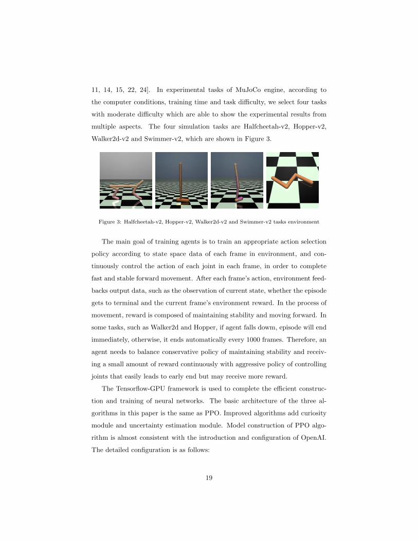
Walker2d-v2 and Swimmer-v2, which are shown in Figure 3.
Figure 3: Halfcheetah-v2, Hopper-v2, Walker2d-v2 and Swimmer-v2 tasks environment
The main goal of training agents is to train an appropriate action selection
policy according to state space data of each frame in environment, and con-
tinuously control the action of each joint in each frame, in order to complete
fast and stable forward movement. After each frame’s action, environment feed-
backs output data, such as the observation of current state, whether the episode
gets to terminal and the current frame’s environment reward. In the process of
movement, reward is composed of maintaining stability and moving forward. In
some tasks, such as Walker2d and Hopper, if agent falls dowm, episode will end
immediately, otherwise, it ends automatically every 1000 frames. Therefore, an
agent needs to balance conservative policy of maintaining stability and receiv-
ing a small amount of reward continuously with aggressive policy of controlling
joints that easily leads to early end but may receive more reward.
The Tensorflow-GPU framework is used to complete the efficient construc-
tion and training of neural networks. The basic architecture of the three al-
gorithms in this paper is the same as PPO. Improved algorithms add curiosity
module and uncertainty estimation module. Model construction of PPO algo-
rithm is almost consistent with the introduction and configuration of OpenAI.
The detailed configuration is as follows:
19

• Policy network. Policy network completes the mapping from state space
S to action spaceA through the three-layer fully connected neural network.
The dimensions of the input layer and output layer are the same as state
space and action space respectively. The dimensions of both the two
hidden full connection layers are 64. Activation function is tanh. Gaussian
action noise is sampled and added to the output layer to complete the
action selection. Loss function based on action selection probability is
shown in formula (8). Learning rate is 0.0003.
• Value function network. Value function network completes the map-
ping of state space S to state value V . Output layer is the one-dimensional
cumulative reward estimation, and the dimensions of both the two hidden
fully connected layers are 64. Activation function is tanh. Mean square
error based on the real reward is used as the loss function to conduct the
supervised learning optimization with a learning rate of 0.001.
• Curiosity network. Curiosity network takes state st and action a as
input and it outputs the state st+1 of the next frame through a 32-
dimensional layer. Activation function is tanh. MSE based on the real
observation state is used as the loss function to optimize the supervised
learning with a learning rate of 0.001.
• Uncertainty estimation network. Uncertainty estimation network for
two states st and st+n as input, with the output for the step estimations
of the number n , and the activation function is tanh. By using mean
square error, supervised learning optimization with learning rate of 0.001
is carried out.
• Other Hyperparameters. Optimization times of each training episode
is 80; discount factor is 0.99; clipping ratio is 0.2.
In certain reinforcement learning experiment, corresponding adjustments ac-
cording to the environment influence training effect. Some optimizations are not
20

appropriate for all tasks, which is one of the reasons for reinforcement learn-
ing training is difficult to reproduce. Optimizations unrelated to algorithms in
previously published literature may affect training results [25, 26, 27]. Such as
data normalization, adding constraints, adjusting initialization settings, etc.
In order to ensure the accuracy and persuasion of the experiment, we would
optimize the algorithm according to the experimental environment and process.
So that our PPO algorithm training effect is better than the results when it was
proposed [9]. The specific treatment is as follows:
• Normalize advantage value. we use value function network to calcu-
late advantage value A, which is used to evaluate the advantage of the
selected action compared with other actions in the same state. Advan-
tage value is also affected by the accuracy of value function network and
real reward. Normalization processing can effectively optimize actions of
the same batch in each episode of training. When reward value in the
task varies greatly, normalization strategy can make whole training pro-
cess more stable, but may increase training bias caused by nonuniform
sampling.
• Data processing. Monte-Carlo method is used for data acquisition and
error calculation. In this method, the reward of each frame affects cumu-
lative reward value of the previous hundred of frames, which also enables
the algorithm to take into account the potential influence of current action
selection in subsequent multiple steps. However, if episode shuts down af-
ter current frame is completed, all subsequent reward will default to 0. A
large bias is also introduced due to a fixed time being reached. This error
not only affects previous frames but is difficult to eliminate. In a fixed
timestep tasks, we set the last frame’s reward as value function network
output. The result improvement compared with the original setting of 0.
• KL divergence constraint. Although the negative effects are alleviated
by ratio clipping of new and old policies, the problem of inappropriate
step size caused by nonuniform sampling is revealed in the advantage
21

value normalization. Therefore, KL divergence constraint is carried out.
If average KL divergence is greater than preset constraint value in current
episode of training, this training episode will be terminated. The preset
value in experiment is 0.015. KL divergence constraint can make training
process more stable.
5.2. Gaussian noise exploration effect experiment
Gaussian noise exploration, as a basic exploration method of policy gradient
algorithm, has certain exploration effect on different continuous action tasks.
The mechanism of dynamically adjusting Gaussian noise based on cumulative
reward can have a stronger exploration scope in early stage of training and
a higher rewarding efficiency in late stage. Here, we compare and verify the
setting of multiple initial Gaussian noise σ of Halfcheetah-v2 and Swimmer-v2
tasks. The experimental results are shown in Figure 4.
Figure 4: Comparison of performance by various Gaussian exploration initial values
Figure 4 shows the performance of experiments on two different tasks with
different initial Gaussian noise σ values. Six different settings are selected for
each task, which can be seen from training trend and reward of different settings:
1) In early stage of training, the smaller exploration scope (i.e., Gaussian
standard deviation) has a better performance (performance in the first 13%
interacts for HalfCheetah and 2% for Swimmer), but at last, premature conver-
gence leads to the suboptimal. Too large Gaussian standard deviation leads to
22
policy degradation, which cannot be optimized to the optimal or takes too much
time. Therefore, the setting of Gaussian noise exploration should be adjusted
from two aspects of training speed and the final performance.
2) Considering factors of speed and performance, it can be clearly found
that in HalfCheetah, the best performance will be achieved if initial value of σ
is set near 0.6. In both 0.5 and 0.7, the performance is significantly damaged.
Relatively in Swimmer, a range of 0.2 to 0.3 would work equally well and con-
verge to optimal value, and with other settings the policy would fall into a local
optimum. Therefore, it is necessary to adjust the action exploration settings
according to specific tasks, as the performance is affected by the exploration
ability which is related to difficulty and type of tasks.
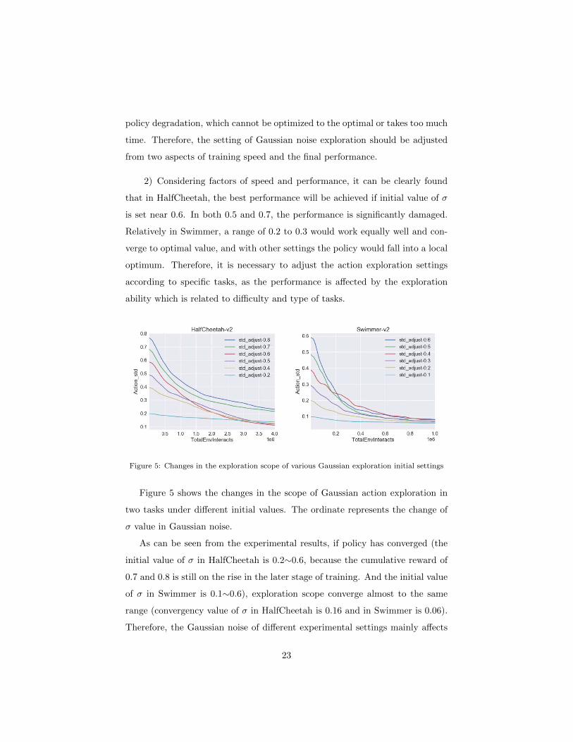
Figure 5: Changes in the exploration scope of various Gaussian exploration initial settings
Figure 5 shows the changes in the scope of Gaussian action exploration in
two tasks under different initial values. The ordinate represents the change of
σ value in Gaussian noise.
As can be seen from the experimental results, if policy has converged (the
initial value of σ in HalfCheetah is 0.2∼0.6, because the cumulative reward of
0.7 and 0.8 is still on the rise in the later stage of training. And the initial value
of σ in Swimmer is 0.1∼0.6), exploration scope converge almost to the same
range (convergency value of σ in HalfCheetah is 0.16 and in Swimmer is 0.06).
Therefore, the Gaussian noise of different experimental settings mainly affects
23
performance by exploration ability and learning progress. The performance will
not affect by the different noise scope after the training convergence.
5.3. Exploration enhancement algorithm experiment
We demonstrate two directional exploration mechanisms. One is curiosity
driven based on prediction error as intrinsic incentive, which is called as ICM-
PPO algorithm. The other is uncertainty measurement based on step size as
intrinsic incentive, which is referred to as IEM-PPO algorithm. We will carry out
a variety of experimental comparison to illustrate effectiveness and advantages.
5.3.1. Exploration enhancement mechanism on training effect
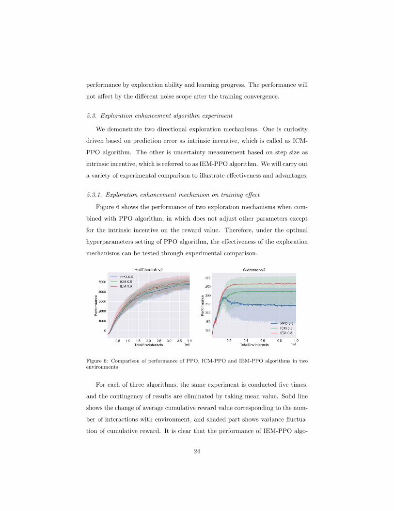
Figure 6 shows the performance of two exploration mechanisms when com-
bined with PPO algorithm, in which does not adjust other parameters except
for the intrinsic incentive on the reward value. Therefore, under the optimal
hyperparameters setting of PPO algorithm, the effectiveness of the exploration
mechanisms can be tested through experimental comparison.
Figure 6: Comparison of performance of PPO, ICM-PPO and IEM-PPO algorithms in twoenvironments
For each of three algorithms, the same experiment is conducted five times,
and the contingency of results are eliminated by taking mean value. Solid line
shows the change of average cumulative reward value corresponding to the num-
ber of interactions with environment, and shaded part shows variance fluctua-
tion of cumulative reward. It is clear that the performance of IEM-PPO algo-
24

rithm is higher than other two algorithms (converging near 5050, 4880, 4800 in
HalfCheetah and 367, 320, 250 in Swimmer), and has better stability in some
tasks (data in Swimmer with a small shadow range).
Thus, it can be concluded that IEM-PPO algorithm is outperforming to both
ICM-PPO and PPO algorithms in terms of training efficiency (performance in
whole training process) and final performance at the end of training. It can
also be seen that the exploration mechanisms such as IEM or ICM can enhance
exploration efficiency without hindering the exploitation effect, so as to obtain
a faster training speed and find a better solution.
5.3.2. Interaction between exploration mechanisms
In the experiment with the same setting as the PPO, the effect of explo-
ration enhancement mechanism is demonstrated. However, theoretically speak-
ing, Gaussian noise can explore around action, but in exploration enhancement
mechanism, the direction of exploration is changed by changing the reward value
of training process. The two exploration mechanisms interact with each other,
exploration enhancement mechanism can ensure Gaussian noise in a smaller
and more accurate scope. In previous Halfcheetah-v2 experiment, it has been
concluded that performance of this task is sensitive to Gaussian noise setting.
Therefore, after adding IEM module here, adjusting Gaussian noise setting will
have a better effect, as shown in Figure 7.
Figure 7: Performance of IEM-PPO algorithm for exploration scope tuning
25

Figure 7 shows IEM-PPO algorithm with adjusting the initial value of Gaus-
sian noise σ to 0.5. It can be seen that after adjusting the initial value, a higher
average cumulative reward (about 5200) is obtained, and a higher performance
is achieved in the whole training process. Therefore, exploration enhancement
mechanism interacts with Gaussian noise, which will have better training effect
after appropriate tuning.
Although the hyperparameter setting can be tuned to achieve better perfor-
mance, the introduction of enhanced exploration model increases complexity of
hyperparameter tuning. In this experiment, it only demonstrates that there are
settings to obtain better performance, we does not search optimal hyperparam-
eter in whole hyperparameter range.
5.3.3. Stability of exploration enhancement mechanism
We demonstrate the stability of our algorithm in this subsection. We employ
Halfcheetah-v2 task for testing because the hyperparameters effects performance
obviously [24]. After comparing performance of various settings, the results are
shown in Table 1.
Table 1 lists the changes of IEM-PPO algorithm and PPO algorithm un-
der different size exploration scope settings. We repeat the experiment three
times for each setting, and the performance is averaged after every 100 episodes.
IEM-PPO algorithm has higher performance in all hyperparameter settings and
has the best convergency value 5252.09. In addition, IEM-PPO algorithm has
5.17%, 23.07%, 18.66% and 5.19% improvements respectively with the compare
of PPO algorithm, and the influence by parameters is slightly lower than the
PPO algorithm (IEM-PPO performances on the initial σ value of 0.6∼0.4 are
all well). Therefore, the algorithm with exploration enhancement mechanism is
more stable.
26

Table 1: Comparison of IEM-PPO and PPO under various settings in Halfcheetah-v2
adjust-0.6 adjust-0.5 adjust-0.4 adjust-0.2
PPO 4824.30 4267.53 4242.58 4084.10
IEM-PPO 5073.83 5252.09 5034.14 4296.04
5.3.4. Experimental effects in more tasks
Through the experiments on Halfcheetach-v2 and Swimmer-v2, we have ex-
plained the influence of exploration enhancement mechanism on the training
performance and stability. Here, we’ll expand into more environments to see
how well the IEM-PPO algorithm fits into various tasks. Because MuJoCo’s
various simulation tasks are different in task objectives, environmental reward
calculation, episode terminal, friction and gravity mechanism, etc. There are
diversified optimization policies in different tasks, which can test the feasibility
of the algorithm in various aspects. The experimental results are shown in Table
2.
Table 2: Comparison of experimental performance of three algorithms in more tasks
HalfCheetah Swimmer Hopper Walker2d
Interacts 4000*1000 2000*500 2000*500 4000*1000
PPOReward 4824.30 242.33 2059.52 2760.64
Variance 544.97 4.55 882.98 1202.87
ICM-PPOReward 4834.10 324.16 2018.37 2801.26
Variance 570.57 2.58 827.87 1213.52
IEM-PPOReward 5073.83 367.74 2158.52 2971.12
Variance 359.92 1.89 770.43 1107.87
Table 2 shows the average performance and variance of various algorithms
in tasks. Among them, the number of interactions with environment in task is
different (4000*1000 and 2000*500), which is mainly determined by the difficulty
of the environment. Moreover, the number of training times in each task has
enabled the policy to converge. All data in table is experiment for three times
27

and get real average reward value in final 100 episodes of policy. It can be seen
that IEM-PPO algorithm is outperforming to other algorithms. Besides having
higher performance, it also has more stable polices and certain generality for
various tasks.
5.3.5. Time complexity of exploreation enhancement mechanism
The exploration enhancement mechanism is designed to identify potential
relationships and trends from the limited available data. In the training process,
the scale of the neural network is increased and the internal incentive needs to be
calculated in each frame, so the training time is longer. Comparison of training
time is shown in Figure 8.
Figure 8: Comparison results of the algorithms in training duration
The total time spent training an agent using different algorithms in Swimmer-
v2 environment is shown in Figure 8. It can be seen that in training process,
the IEM-PPO and ICM-PPO algorithms need longer computing time, but both
of them are proportional based on environmental interactions. Therefore, al-
though enhancement mechanisms has increased the computational burden of
the training process, it has the same complexity with PPO algorithm, and com-
putational time is still within the acceptable range. Note that training time
is not only affected by algorithm framework, but also affected by environment
complexity, hardware computing speed and code implementation efficiency.
28

6. Conclusion and Future Work
In this paper, we propose a new algorithm based on exploration enhancement
mechanism, and demonstrate algorithm effects in continuous action tasks.
Firstly, we theoretically analyze the function and defect of Gaussian explo-
ration mechanism in training process of PPO algorithm. From practical view,
experimental verification of various exploration scope settings shows that appro-
priate and efficient exploration settings should be adopted to ensure performance
for different environments.
Then, from the perspective of improving efficiency of algorithm exploration,
ICM-PPO algorithm based on curiosity driven exploration is implemented and
IEM-PPO algorithm based on uncertainty estimation is proposed. Based on un-
certainty estimation theory, IEM-PPO algorithm uses collected environmental
state data to construct neural network to complete the uncertainty estimation
function, using uncertainty estimation as internal incentive to carry out positive
incentive for the action exploration. We ensures efficient exploration under the
condition of considering training time.
In experiment, we use PPO algorithm and ICM-PPO algorithm for compari-
son with IEM-PPO algorithm on Mujoco physical simulation environment. Con-
sidering the exploration ability, IEM-PPO algorithm improves training speed
and final training performance. In terms of stability, exploration enhancement
mechanism is applicable in most parameter settings and has stability. In training
time, the new neural network increases the scale of the model and the number
of parameters in the model which requires longer training time but not increases
too much computing burden.
We can conclude that although IEM-PPO algorithm requires longer training
time, it has excellent training efficiency and performance, and has stability and
robustness.
Future work can be explored from the following three aspects:
1) In discrete action tasks, if the optimal action distribution is bimodal
or multimodal, policy gradient algorithm will have better effect. However, the
29

Gaussian distribution in continuous action tasks can only be a single peak, which
cannot give full play to the potential advantages of policy gradient algorithm.
2) The dimension of internal incentive is not consistent with extrinsic re-
ward. For reinforcement learning task, variation range of reward corresponding
to the good and bad policies also affects the effect of the exploration enhance-
ment mechanism. Therefore, a general strategy is needed to solve hyperparam-
eter optimization problem [28, 24].
3) It may be better to use the characteristics of multi-agent learning for
further exploration [29, 30, 31], but the current multi-agent learning is weaker
than single agent under the same amount of training, so it is necessary to balance
the optimization objectives of multi-agents in an appropriate way.
Acknowledgement
This work was supported by the National Key R&D Program of China un-
der Grant No. 2017YFB1003103; the National Natural Science Foundation
of China under Grant Nos. 61300049, 61763003; and the Natural Science Re-
search Foundation of Jilin Province of China under Grant Nos. 20180101053JC,
20190201193JC.
References
[1] M. Hessel, J. Modayil, H. van Hasselt, T. Schaul, G. Ostrovski, W. Dabney,
D. Horgan, B. Piot, M. G. Azar, D. Silver, Rainbow: Combining improve-
ments in deep reinforcement learning, In AAAI Conference on Artificial
Intelligence (2018) 3215–3222.
[2] H. van Hasselt, A. Guez, D. Silver, Deep reinforcement learning with double
q-learning, In AAAI Conference on Artificial Intelligence (2016) 2094–2100.
[3] T. Haarnoja, A. Zhou, P. Abbeel, S. Levine, Soft actor-critic: Off-policy
maximum entropy deep reinforcement learning with a stochastic actor, In
International Conference on Machine Learning (2018) 1856–1865.
30

[4] Y. Wu, E. Mansimov, R. B. Grosse, S. Liao, J. Ba, Scalable trust-region
method for deep reinforcement learning using kronecker-factored approxi-
mation, In Neural Information Processing Systems (2017) 5279–5288.
[5] A. R. Mahmood, D. Korenkevych, G. Vasan, W. Ma, J. Bergstra, Bench-
marking reinforcement learning algorithms on real-world robots, In Con-
ference on Robot Learning (2018) 561–591.
[6] J. Li, L. Yao, X. Xu, B. Cheng, J. Ren, Deep reinforcement learning for
pedestrian collision avoidance and human-machine cooperative driving, In-
formation Sciences 532 (2020) 110–124.
[7] S. Gu, T. P. Lillicrap, I. Sutskever, S. Levine, Continuous deep q-learning
with model-based acceleration, In International Conference on Machine
Learning (2016) 2829–2838.
[8] S. Iqbal, F. Sha, Actor-attention-critic for multi-agent reinforcement learn-
ing, In International Conference on Machine Learning (2019) 2961–2970.
[9] J. Schulman, F. Wolski, P. Dhariwal, A. Radford, O. Klimov, Proximal
policy optimization algorithms, CoRR abs/1707.06347 (2017).
[10] A. Ilyas, L. Engstrom, S. Santurkar, D. Tsipras, F. Janoos, L. Rudolph,
A. Madry, Are deep policy gradient algorithms truly policy gradient algo-
rithms?, CoRR abs/1811.02553 (2018).
[11] K. Ciosek, Q. Vuong, R. Loftin, K. Hofmann, Better exploration with opti-
mistic actor critic, In Neural Information Processing Systems (2019) 1785–
1796.
[12] D. Pathak, P. Agrawal, A. A. Efros, T. Darrell, Curiosity-driven explo-
ration by self-supervised prediction, In International Conference on Ma-
chine Learning (2017) 2778–2787.
[13] V. Mnih, K. Kavukcuoglu, D. Silver, A. A. Rusu, J. Veness, M. G. Belle-
mare, A. Graves, M. A. Riedmiller, A. Fidjeland, G. Ostrovski, S. Petersen,
31

C. Beattie, A. Sadik, I. Antonoglou, H. King, D. Kumaran, D. Wierstra,
S. Legg, D. Hassabis, Human-level control through deep reinforcement
learning, Nature (7540) (2015) 529–533.
[14] T. P. Lillicrap, J. J. Hunt, A. Pritzel, N. Heess, T. Erez, Y. Tassa, D. Sil-
ver, D. Wierstra, Continuous control with deep reinforcement learning, In
International Conference on Learning Representations (2016) Poster.
[15] V. Mnih, A. P. Badia, M. Mirza, A. Graves, T. P. Lillicrap, T. Harley,
D. Silver, K. Kavukcuoglu, Asynchronous methods for deep reinforcement
learning, In International Conference on Machine Learning (2016) 1928–
1937.
[16] Y. Burda, H. Edwards, D. Pathak, A. J. Storkey, T. Darrell, A. A. Efros,
Large-scale study of curiosity-driven learning, In International Conference
on Learning Representations (2019) Poster.
[17] P. Auer, N. Cesa-Bianchi, P. Fischer, Finite-time analysis of the multiarmed
bandit problem, Machine Learning (2-3) (2002) 235–256.
[18] A. L. Strehl, M. L. Littman, An analysis of model-based interval estima-
tion for markov decision processes, Journal of Computer and System Sci-
ences (8) (2008) 1309–1331.
[19] M. Fortunato, M. G. Azar, B. Piot, J. Menick, M. Hessel, I. Osband,
A. Graves, V. Mnih, R. Munos, D. Hassabis, O. Pietquin, C. Blundell,
S. Legg, Noisy networks for exploration, In International Conference on
Learning Representations (2018) Poster.
[20] R. S. Sutton, D. A. McAllester, S. P. Singh, Y. Mansour, Policy gradient
methods for reinforcement learning with function approximation, In Neural
Information Processing Systems (1999) 1057–1063.
[21] X. Xu, L. Zuo, Z. Huang, Reinforcement learning algorithms with function
approximation: Recent advances and applications, Information Sciences
261 (2014) 1–31.
32

[22] J. Schulman, P. Moritz, S. Levine, M. I. Jordan, P. Abbeel, High-
dimensional continuous control using generalized advantage estimation, In
International Conference on Learning Representations (2016) Poster.
[23] E. Todorov, Convex and analytically-invertible dynamics with contacts and
constraints: Theory and implementation in mujoco, In International Con-
ference on Robotics and Automation (2014) 6054–6061.
[24] L. Pinto, J. Davidson, R. Sukthankar, A. Gupta, Robust adversarial re-
inforcement learning, In International Conference on Machine Learning
(2017) 2817–2826.
[25] Y. Gao, L. Chen, B. Li, Post: Device placement with cross-entropy mini-
mization and proximal policy optimization, In Neural Information Process-
ing Systems (2018) 9993–10002.
[26] B. Liu, Q. Cai, Z. Yang, Z. Wang, Neural proximal/trust region policy
optimization attains globally optimal policy, CoRR abs/1906.10306 (2019).
[27] D. Ye, Z. Liu, M. Sun, B. Shi, P. Zhao, H. Wu, H. Yu, S. Yang, X. Wu,
Q. Guo, Q. Chen, Y. Yin, H. Zhang, T. Shi, L. Wang, Q. Fu, W. Yang,
L. Huang, Mastering complex control in MOBA games with deep rein-
forcement learning, In AAAI Conference on Artificial Intelligence (2020)
6672–6679.
[28] D. Zha, K. Lai, K. Zhou, X. Hu, Experience replay optimization, In Inter-
national Joint Conference on Artificial Intelligence (2019) 4243–4249.
[29] J. Song, H. Ren, D. Sadigh, S. Ermon, Multi-agent generative adversarial
imitation learning, In Neural Information Processing Systems (2018) 7472–
7483.
[30] T. Salimans, J. Ho, X. Chen, I. Sutskever, Evolution strategies as a scalable
alternative to reinforcement learning, CoRR abs/1703.03864 (2017).
33

[31] H. Wang, X. Wang, X. Hu, X. Zhang, M. Gu, A multi-agent reinforcement
learning approach to dynamic service composition, Information Sciences
363 (2016) 96–119.
34