Embed Size (px)
Citation preview

A Model and Case Study for Efficient Shelf Usage and
Assortment Analysis
M. Murat Fadıloglu∗
Oya Ekin Karasan †
Mustafa C. Pınar‡
Department of Industrial Engineering
Bilkent University
06800 Ankara, Turkey.
May 15, 2007
Abstract
In the rapidly changing environment of Fast Moving Consumer Goods sector where new prod-
uct launches are frequent, retail channels need to reallocate their shelf spaces intelligently while
keeping up their total profit margins, and to simultaneously avoid product pollution. In this paper
we propose an optimization model which yields the optimal product mix on the shelf in terms
of profitability, and thus helps the retailers to use their shelves more effectively. The model is
applied to the shampoo product class at two regional supermarket chains. The results reveal not
only a computationally viable model, but also substantial potential increases in the profitability
after the reorganization of the product list.
Key words: retailing, assortment optimization, demand substitution.
1 Introduction
One of the critical issues in Fast Moving Consumer Goods (FMCG) sector is the rapid pace of the
business where new retail products are launched frequently. Firms operating in this sector are forced
to adopt operational strategies that would enable them to keep up with the fast changing market∗[email protected], corresponding author†[email protected]‡[email protected]
1

conditions. At the retail store level, the new products have to share common shelf space with the
already existing products. The sheer increase in the number of different products or SKUs (SKU: stock
keeping units as they are called in the sector) causes product pollution in stores. On the other hand,
the firms supplying retail stores are looking for ways to increase their visibility through proliferating
their SKUs to conquer shelf space. Both of these phenomena force retailers to eliminate certain SKUs
from their shelves in favor of others. However, the criteria used in this elimination/replacement are
not entirely clear.
This study was initiated after we were approached by the local office of an international FMCG
conglomerate. They complained that the product pollution, which is especially acute in the small and
medium size retailers, was hurting their sales. They stated that these retailers are not aware of the
phenomenon and its repercussions on their own profitability. Since the retailers were not taking any
measures about the unreasonable number of SKUs they are carrying on their shelf space, they were
also not allowing the products of this FMCG conglomerate to realize their full potential on this retail
channel. They believed that sales they were losing was more significant compared to other producers,
since they were the market leaders in most product categories. The local office request was for us
to develop a tool that the retailers could use to optimize their product mix on their shelves, which
would also quantify the gain they can achieve by eliminating some SKUs. If the retailers implemented
the recommendations of such a tool, this would reduce the product pollution and thereby, indirectly,
benefit the sales of the conglomerate.
Against this background the purpose of the present paper is to develop a viable optimization
model which would prevent product pollution and simultaneously achieve an efficient assortment by
judicious partitioning of the shelf space among the variety of products. The model is applied to
a specific hair care product class (shampoo) in two local chain stores and tested with actual data.
The results summarized in the paper have been conveyed to the retail chains’ managements and the
resulting tool has been presented for their use.
Our contribution in this paper is an optimization model that improves the product mix on the
shelf for any given product class at a retailer. There are many models in the literature with the same
purpose. Yet, most models are complicated and have extensive data requirements. We claim that our
model needs minimal data and can be used at/by almost any retailer that keeps track of their sales
without complication. This model should be applicable to many smaller size retailers at which limited
data is available.
The rest of this paper is organized as follows. In Section 2 we provide a brief overview of the
related literature. Section 3 is devoted to the description and discussion of our model. A case study
and results are reported in Section 4. Possible extensions and conclusions are given in Section 5.
2

2 Literature Review
The literature in the area of assortment management is quite large. We refer the readers to Mahajan
and van Ryzin (1998) and Kok et al. (2005) for extensive reviews. Here we provide a brief review of
the literature directly related to our manuscript.
An important work by Corstjen and Doyle (1981) provides an optimization model for shelf space
allocation assuming a multiplicative self and cross space elasticity structure. They propose store
experiments in order to estimate the parameters of their complicated elasticity structure. Since their
estimation procedure is not practically viable, its applicability is limited. Inventory considerations are
omitted in this model as is the case in ours. Urban (1998) extends it to cover inventory considerations
as well.
A critical part of our model is the assumption that the customers who cannot find the SKU of
their preference will substitute that SKU with another one. In our study, we assume that substitution
occurs within product categories. A version (without the categories) of such substitution can be
observed in inventory models incorporating demand substitution (see Netessine and Rudi (2003) and
references therein). van Ryzin and Mahajan (1999) propose a newsboy model to determine the
purchase quantities of different SKUs within a category. The paper makes use of a multinomial logit
choice model to determine the individual purchase decisions. Each customer may choose to purchase
among the listed products or may choose not to puchase anything. If the product of their choice in
not available, the sale is lost. They show that the optimal assortment has a simple structure for their
stylistic model in which the unit prices are identical. Majahan and van Ryzin (2001) also allow dynamic
substitution to occur when the SKU demanded is not in stock and use sample path analysis to obtain
structural results. Smith and Agrawal (2000) investigate the effect of substitution on the optimal
base-stock levels in multi-item inventory systems. Their formulation leads to an integer program.
Cachon et al. (2005) also incorporate customer search into the choice model which is similar to the
one in van Ryzin and Mahajan (1999). There are also many papers in the literature that consider the
determination of the optimal stocking levels given that assortment is already selected.
In a recent work, Kok and Fisher (2006) provide an assortment optimization model that takes into
account the effect of shelf space allocation on customer choice as well as the effect of inventory policy
on stockout based substitutions. Their model is quite elaborate and has extensive data requirements.
In the paper, they also develop a procedure for the estimation of demand and substitution parameters
and an iterative heuristic for the optimization model. They finally present the results of the application
of their method, to a supermarket chain.
Our work is akin to the one of Kok and Fisher (2006), in the sense that we provide a tool that can
be remotely applied in retailers and we present its application at two supermarket chains. However,
3

our model is considerably simpler in terms of its structure. It does not take into account the elasticity
of demand to shelf space nor the effects of the inventory policy. The supermarkets for which we
devised our model do not have access to the kind of data necessary for the application of the method
by Kok and Fisher (2006). We could only access monthly sales and price data. Our model provides
a simple tool to exploit what is available in such settings.
3 Model
We group the products into categories according to their quality levels and prices. We assume K
product categories are available. For convenience of presentation we define the category set K =
{1, . . . , K} and the SKU set within each category i ∈ K , Ni = {1, . . . , Ni} .
We make the following important modeling assumption: when a SKU is taken off the shelf an
estimated portion of the demand for that SKU is distributed to other SKUs. This portion is determined
according to a “substitution ratio” s . The specific computation of this parameter for our target
application is described in detail in Section 4.
We will assume that the following data from the retail stores are available for our model:
• The SKU list for on-shelf products at each category,
• Sales data for a predetermined time horizon for each SKU in each category,
• Profit margins of each SKU in each category,
• Probability (frequency) of buying another SKU from the same retailer when a given SKU is not
carried in that retailer.
The cost of keeping one SKU on the shelf per period is referred to as c , and is assumed to be
given. We discuss the meaning of this parameter and its estimation below.
Our model aims to find the optimum SKU list to be kept on shelf at retailers so as to maximize
the total average profit per period. Therefore, the goal is to decide which SKUs to eliminate from the
list to minimize product pollution on the shelves while maximizing total profit. Now, we describe the
ingredients of the model.
Parameters:
• qij : average sales data per period for SKU j of category i ,
• Ti : total sales per period in category i : Ti =∑Ni
j=1 qij ,
• pij : profit obtained when one unit of SKU j of category i is sold,
4

• c : cost per period of keeping one SKU on the shelf,
• si : substitution ratio for category i ,
• d : minimum ratio for directly satisfied demand at each category, referred to as the minimum
conservation ratio.
Decision Variables: Our decision variables are defined as follows:
• The decision to keep SKU i in category j is modeled using a binary variable:
xij =
⎧⎨⎩ 1 SKU j of category i is kept in the list
0 otherwise(1)
• Ui : total lost sales in category i
• qij : average estimated sales for SKU j of category i after substitution effect
Constraints: The constraints of our model, some of which are of a definitional nature, and
therefore given only for convenience in the presentation, are defined as follows:
• Constraint to ensure that ratio of demand corresponding to undeleted SKUs to the total demand
be no less than minimum conservation ratio d for each category i :
Ni∑j=1
qijxij ≥ d Ti for all i ∈ K, (2)
• Definition of total lost sales per period in category i due to unlisting:
Ui = Ti −Ni∑j=1
xijqij for all i ∈ K, (3)
• Definition of average estimated sales per period for SKU j in category i after substitution:
qij = qij +siUiqij
Ti − Uifor all i ∈ K and j ∈ Ni, (4)
Our objective function consists of the difference of the total estimated profit after SKU elimination
and the total cost of keeping the selected SKUs on the shelf:
Zdef=
K∑i=1
Ni∑j=1
pij qijxij − c
K∑i=1
Ni∑j=1
xij (5)
Now, we are ready to define the optimization model for deciding the optimal SKU list that maximizes
the total projected profit after substitution as choosing the values of the decision variables xij , Ui, qij
satisfying the constraints above and maximizing (5), i.e., as the model:
maxxij ,Ui,qij
Z subject to (1) − (2) − (3) − (4). (6)
5
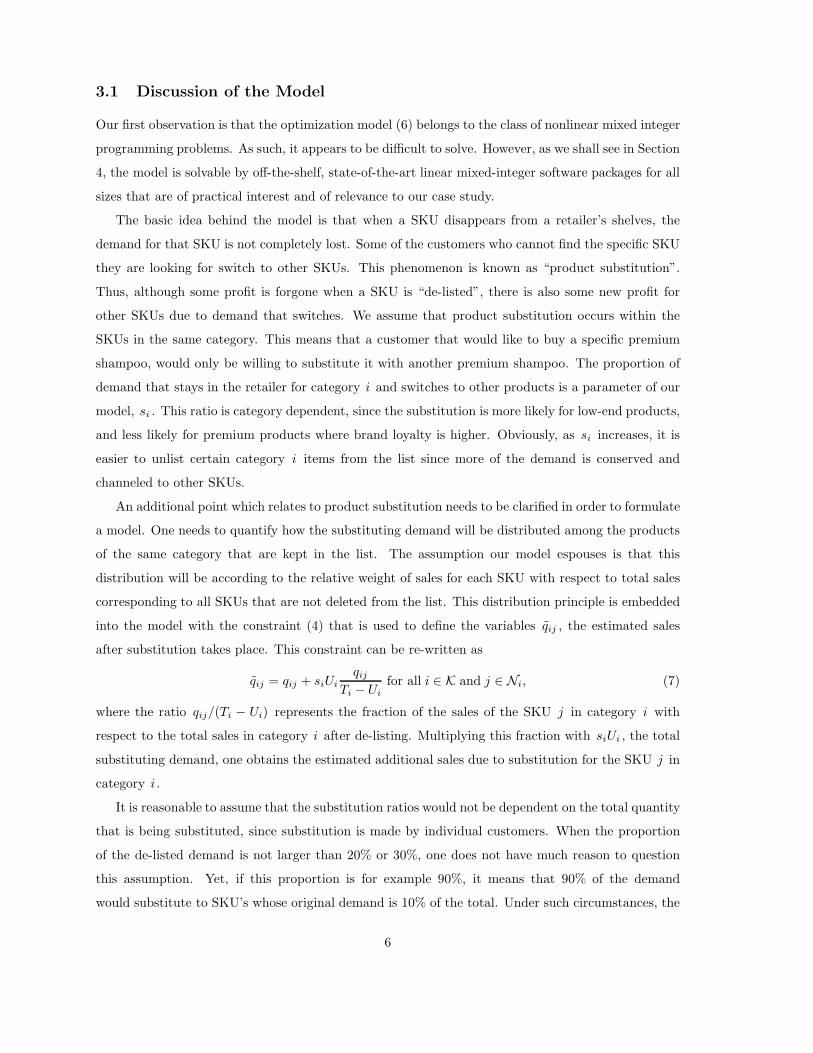
3.1 Discussion of the Model
Our first observation is that the optimization model (6) belongs to the class of nonlinear mixed integer
programming problems. As such, it appears to be difficult to solve. However, as we shall see in Section
4, the model is solvable by off-the-shelf, state-of-the-art linear mixed-integer software packages for all
sizes that are of practical interest and of relevance to our case study.
The basic idea behind the model is that when a SKU disappears from a retailer’s shelves, the
demand for that SKU is not completely lost. Some of the customers who cannot find the specific SKU
they are looking for switch to other SKUs. This phenomenon is known as “product substitution”.
Thus, although some profit is forgone when a SKU is “de-listed”, there is also some new profit for
other SKUs due to demand that switches. We assume that product substitution occurs within the
SKUs in the same category. This means that a customer that would like to buy a specific premium
shampoo, would only be willing to substitute it with another premium shampoo. The proportion of
demand that stays in the retailer for category i and switches to other products is a parameter of our
model, si . This ratio is category dependent, since the substitution is more likely for low-end products,
and less likely for premium products where brand loyalty is higher. Obviously, as si increases, it is
easier to unlist certain category i items from the list since more of the demand is conserved and
channeled to other SKUs.
An additional point which relates to product substitution needs to be clarified in order to formulate
a model. One needs to quantify how the substituting demand will be distributed among the products
of the same category that are kept in the list. The assumption our model espouses is that this
distribution will be according to the relative weight of sales for each SKU with respect to total sales
corresponding to all SKUs that are not deleted from the list. This distribution principle is embedded
into the model with the constraint (4) that is used to define the variables qij , the estimated sales
after substitution takes place. This constraint can be re-written as
qij = qij + siUiqij
Ti − Uifor all i ∈ K and j ∈ Ni, (7)
where the ratio qij/(Ti − Ui) represents the fraction of the sales of the SKU j in category i with
respect to the total sales in category i after de-listing. Multiplying this fraction with siUi , the total
substituting demand, one obtains the estimated additional sales due to substitution for the SKU j in
category i .
It is reasonable to assume that the substitution ratios would not be dependent on the total quantity
that is being substituted, since substitution is made by individual customers. When the proportion
of the de-listed demand is not larger than 20% or 30%, one does not have much reason to question
this assumption. Yet, if this proportion is for example 90%, it means that 90% of the demand
would substitute to SKU’s whose original demand is 10% of the total. Under such circumstances, the
6

customer base would probably not be happy with the product mix presented on the retailer’s shelves
and the actual substution ratio would be lower. Moreover, since such a policy of satisfying only a
small portion of customers’ original demand would be detrimental for the image of the retailer, it is
reasonable to assume that the model should have a bound on the ratio of the substituting demand.
The minimum conservation ratio in our model represents this bound on the ratio of substituting
demand for each category, as expressed in (2). The constraint in (2) ensures that the model does not
suggest solutions in the region where modeling assumptions begin to break.
Another critical component of our model is the cost of keeping SKUs on shelf, which is linear on the
number of SKUs on shelf. In the small and medium size retailers where our study was concentrated,
we observed that there were quite a few SKUs with very small sale volumes. With such small sale
volumes, they should not be worth the effort of organizing them on the shelf, keeping track of their
inventories etc. Moreover, we realized that if such SKUs could be eliminated there would be drastic
reduction in terms of the product pollution. Thus, c models all these indirect costs that are due to
keeping one SKU on the list. Since this cost cannot be directly estimated by accounting methods,
it has to be determined by asking the retail managers appropriate questions. It is obvious that as c
increases, more elimination would take place and the optimal list would shrink.
Since most of the model constraints are of definitional nature, it is possible to collapse the con-
straints (3) and (4) into the objective function and obtain a more concise model. This concise form
is instrumental in proving the results provided in the following sections, and it is presented below:
max Zdef=
K∑i=1
Ni∑j=1
⎛⎝(pijqij(1 − si) − c)xij + si
⎛⎝ Ni∑
j=1
qij
⎞⎠∑j pijqijxij∑
j qijxij
⎞⎠ (8)
subject toNi∑j=1
qijxij ≥ d Ti for all i ∈ K, xij ∈ {0, 1} for all i ∈ K, j ∈ Ni. (9)
As can be seen in (8), the cost components that correspond to each category are simply added up
to constitute the objective function. Moreover, the constraints of the optimization model given in (9)
only involve the decision variables of a single category at a time. Thus, our model can be decomposed
into K independent problems for each i = 1, . . . , K :
max Zidef=
Ni∑j=1
⎛⎝(pijqij(1 − si) − c)xij + si
⎛⎝ Ni∑
j=1
qij
⎞⎠∑j pijqijxij∑
j qijxij
⎞⎠ (10)
subject toNi∑j=1
qijxij ≥ d Ti, xij ∈ {0, 1} for all j ∈ Ni. (11)
We note that the original model (6) and the collapsed and decomposed model (10)-(11) are both
non-convex and non-concave (neither quasi-convex nor quasi-concave) maximization problems over a
7

set of integers. As such, they look quite difficult for numerical processing. Interestingly, a continuous
relaxation that is immediately obtained by relaxing the integer (binary) requirement on the variables
xij does not yield a tractable problem either, in the sense that the resulting maximization problem
is not guaranteed to have neither quasi-convex, nor quasi-concave objective function. To see this, let
us observe that the decomposed problem (10)-(11) for category i can be re-written in vector-matrix
notation as
max Zi = fT x +hT x
qT x(12)
subject to qT x ≥ d Ti, 0 ≤ x ≤ e. (13)
where f ∈ RNi with component j equal to qijpij(1 − si) − c , h ∈ R
Ni with component j equal to
siTipijqij and q ∈ RNi with components qij , while x ∈ R
Ni denotes the vector with components
xij , for all j ∈ Ni . We note immediately that the continuous relaxation model (12)-(13) would be
equivalent to a linear programming problem were it not for the presence of the term fT x in the
objective function. Without that term, the problem would fall into the realm of linear-fractional
maximization with a quasi-convex and quasi-concave (hence, quasi-linear) objective function over
a polyhedral set. It is well-known that such problems are easily transformed to equivalent linear
programs. However, the presence of the term fT x renders the objective function neither quasi-convex,
nor quasi-concave in general (see [8] for conditions regarding quasi-convexity or quasi-concavity of such
functions). To see this, let us consider the level sets of the objective function
Sα = {x ∈ RNi : fT x +
hT x
qT x≤ α}
for some scalar α ∈ R . Notice that the positivity of the denominator is guaranteed from the constraint
qT x ≥ d Ti . Therefore, an equivalent expression for Sα is given by {x ∈ RNi : (qT x)(fT x) + hT x −
αqT x ≤ 0} . Equivalently, we have
Sα = {x ∈ RNi : xT
(fqT + qfT
2
)x + hT x − αqT x ≤ 0}.
By definition of quasi-convexity, the set Sα should be a convex set. However, for this to hold true,
one needs to guarantee positive semi-definiteness of the rank-2 matrix fqT +qfT
2 , which is not true in
general. A similar discussion with the sub-level sets {x ∈ RNi : fT x + hT x
qT x ≥ α} encounters the same
conclusion.
Therefore, even the continuous relaxation of our model does not seem to be, at least from a
theoretical point of view, an easy continuous optimization problem. Nonetheless, in the sequel, we
shall reveal several interesting features of the nonlinear model along with a careful linearization that
contribute to its numerical solution in reasonable running times. These features include a property
8
of the local optima of the problem, bounds for preprocessing, the special case of uniform profit, and
finally an effective linearization scheme.
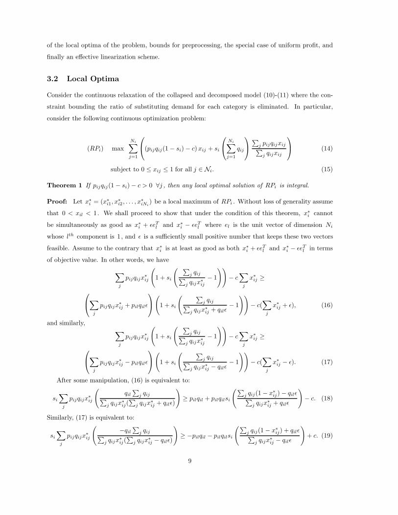
3.2 Local Optima
Consider the continuous relaxation of the collapsed and decomposed model (10)-(11) where the con-
straint bounding the ratio of substituting demand for each category is eliminated. In particular,
consider the following continuous optimization problem:
(RPi) maxNi∑j=1
⎛⎝(pijqij(1 − si) − c)xij + si
⎛⎝ Ni∑
j=1
qij
⎞⎠ ∑j pijqijxij∑
j qijxij
⎞⎠ (14)
subject to 0 ≤ xij ≤ 1 for all j ∈ Ni. (15)
Theorem 1 If pijqij(1 − si) − c > 0 ∀j , then any local optimal solution of RPi is integral.
Proof: Let x∗i = (x∗
i1, x∗i2, . . . , x
∗iNi
) be a local maximum of RPi . Without loss of generality assume
that 0 < xil < 1. We shall proceed to show that under the condition of this theorem, x∗i cannot
be simultaneously as good as x∗i + εeT
l and x∗i − εeT
l where el is the unit vector of dimension Ni
whose lth component is 1, and ε is a sufficiently small positive number that keeps these two vectors
feasible. Assume to the contrary that x∗i is at least as good as both x∗
i + εeTl and x∗
i − εeTl in terms
of objective value. In other words, we have
∑j
pijqijx∗ij
(1 + si
( ∑j qij∑
j qijx∗ij
− 1
))− c
∑j
x∗ij ≥
⎛⎝∑
j
pijqijx∗ij + pilqilε
⎞⎠(
1 + si
( ∑j qij∑
j qijx∗ij + qilε
− 1
))− c(
∑j
x∗ij + ε), (16)
and similarly, ∑j
pijqijx∗ij
(1 + si
( ∑j qij∑
j qijx∗ij
− 1
))− c
∑j
x∗ij ≥
⎛⎝∑
j
pijqijx∗ij − pilqilε
⎞⎠(
1 + si
( ∑j qij∑
j qijx∗ij − qilε
− 1
))− c(
∑j
x∗ij − ε). (17)
After some manipulation, (16) is equivalent to:
si
∑j
pijqijx∗ij
(qil
∑j qij∑
j qijx∗ij(∑
j qijx∗ij + qilε)
)≥ pilqil + pilqilsi
(∑j qij(1 − x∗
ij) − qilε∑j qijx∗
ij + qilε
)− c. (18)
Similarly, (17) is equivalent to:
si
∑j
pijqijx∗ij
(−qil
∑j qij∑
j qijx∗ij(∑
j qijx∗ij − qilε)
)≥ −pilqil − pilqilsi
(∑j qij(1 − x∗
ij) + qilε∑j qijx∗
ij − qilε
)+ c. (19)
9

Now, from (18) and (19) we have:⎛⎝∑
j
qijx∗ij(∑
j
qijx∗ij + qilε)
⎞⎠(pilqil + pilqilsi
(∑j qij(1 − x∗
ij) − qilε∑j qijx∗
ij + qilε
)− c
)≤ qilsi
∑j
pijqijx∗ij
∑j
qij ≤
⎛⎝∑
j
qijx∗ij(∑
j
qijx∗ij − qilε)
⎞⎠(pilqil + pilqilsi
(∑j qij(1 − x∗
ij) + qilε∑j qijx∗
ij − qilε
)− c
)(20)
which is, after some simplifications, equivalent to
pilqil(1 − si) − c ≤ 0,
leading to a contradiction.
Interestingly the quantity pijqij(1 − si) − c that decides the integrality of local optima in the
relaxed problem also appears in the discussion of the uniform profit case (Section 3.4). This quantity
is instrumental in solving the problem in the uniform profit case. While it is hard to give a precise
economic interpretation to this quantity, we can view it as a modified profit coefficient.
3.3 Bounds for Pre-processing
Now, we investigate lower and upper bounds on the change in the objective function value when we
include a SKU in the list of SKUs on the shelf, while keeping everything else fixed. In other words, we
assume to have a feasible vector x and concentrate on the item i, � . We investigate the effect ΔZi,�
on the objective function of making xi,� equal to one. Throughout this section, we use the collapsed
and decomposed model (10)-(11).
Lemma 1
ΔZi� = pi�qi�
(1 + si
( ∑j qij∑
j �=� qijxij + qi�− 1
))− c − qi�si
((∑
j qij)(∑
j �=� pijqijxij)(∑
j �=� qijxij + qi�)(∑
j �=� qijxij)
).
Proof: After writing out the difference between the objective function values corresponding to the
cases where xi,� = 0 and xi,� = 1, respectively, we obtain
ΔZi� = pi�qi�
(1 + si
( ∑j qij∑
j �=� qijxij + qi�− 1
))− c +
si
⎛⎝∑
j
qij
⎞⎠⎛⎝∑
j �=�
pijqijxij
⎞⎠( 1∑
j �=� qijxij + qi�− 1∑
j �=� qijxij
).
After some manipulation, Lemma 1 is obtained.
10

Proposition 1
pi�qi� − c − qi�si
d(max
jpij) ≤ ΔZi� ≤ pi�qi�
(1 + si
1 − d
d
)− c − qi�si(min
jpij).
Proof: From Constraint 2 we know that
∑j
qij ≥∑
j
qijxij ≥ d∑
j
qij .
Therefore, we can give the following upper bound on ΔZi� :
ΔZi� ≤ pi�qi�
(1 + si
( ∑j qij
d∑
j qij− 1
))− c − qi�si
(∑
j qij)(∑
j �=� pijqijxij)(∑
j qij)(∑
j �=� qijxij).
Since∑
j �=� pijqijxij ≥ (minj pij)∑
j �=� qijxij , we obtain:
ΔZi� ≤ pi�qi�
(1 + si
1 − d
d
)− c − qi�si(min
jpij).
Similarly, we can establish the lower bound
ΔZi� ≥ pi�qi� − c − qi�si
d(max
jpij).
One can observe that the values of certain variables in the optimal solution can be determined by
just checking the problem parameters based on the lower bound presented in the following proposi-
tion. This gives rise to the rule presented in Proposition 2. This rule is used for preprocessing the
optimization model in order to reduce the problem size.
Proposition 2 If the lower bound on Δzi� is positive or zero, i.e.,
pi�qi� − c − qi�si
d(max
jpij) ≥ 0
then SKU � of category i is guaranteed to be in an optimal list, i.e., we can set xi� = 1 without loss
of optimality.
This proposition stipulates that the SKU � in category i should be kept in the list, if the cor-
responding lower bound is greater or equal to zero. This is due to fact if this SKU is added to the
list the objective function will improve by at least the value of the lower bound, irrespective of the
composition of the list. Since adding an additional SKU to the list cannot violate any constraint of
the program, we are never worse off when that SKU is in the list.
One can think of a similar proposition using the upper bound which would stipulate that a SKU
should be kept off the list if the corresponding upper bound is nonpositive. Yet, the problem is that
11

by keeping a SKU out of the list one can violate constraint (11). Thus, such an elimination can only
be done if this constraint is nonbinding at the optimal point. Since this requires post-optimization
processing, its use in pre-processing would be complicated. Still if constraint (11) is superfluous, i.e.,
d = 0, then the upper bound would also yield a pre-processing rule.
3.4 A Special Case: Uniform Profit
In this section, we present how the model simplifies when the profit margins are equal for each SKU
within a category, i.e. when pij = pi for all j = 1, . . . , Ni . Under this condition the objective function
of the decomposed problem given in (10), would simplify to
Zi =∑
j
(pi(1 − si)qij − c)xij + pisi
∑j
qij (21)
If it were not for the constraint (11), in this setting the optimization problem would decompose
to Ni independent subproblems involving one SKU at a time. This gives rise to the next proposition
where x∗ denotes an optimal solution and xc denotes a candidate solution. Let Δuij = pi(1−si)qij−c .
Proposition 3
1. For each j ∈ Ni if Δuij ≥ 0 then set xc
ij = 1 , otherwise set xcij = 0 .
2. If∑
j qijxcij ≥ d
∑j qij then x∗
ij = xcij .
3. If∑
j qijxcij < d
∑j qij then use the following procedure:
(a) Sort those indices j ∈ Ni , in descending order according to the quotient Δuij/qij . Let jl
denote the corresponding index in the original list of the lth element in the sorted list.
(b) Find l∗ as the minimum l satisfying∑l
m=1 qijm ≥ d∑Ni
j=1 qij .
(c) Set xijl= 1 for l = 1, . . . , l∗ ; xijl
= 0 for l = l∗ + 1, . . . , Ni .
The proposition states that the candidate solution based on the optimal solutions of the Ni sub-
problems would be optimal for the overall problem for category i , if constraint (11) is satisfied. In
the case where constraint (11) is violated by the candidate solution, one needs to set a larger number
of variables to one, which is achieved by means of the simple procedure described in the proposi-
tion. In the latter case, one deals essentially with a reverse knapsack-type problem, and the proposed
procedure is typical for this class of problems.
12
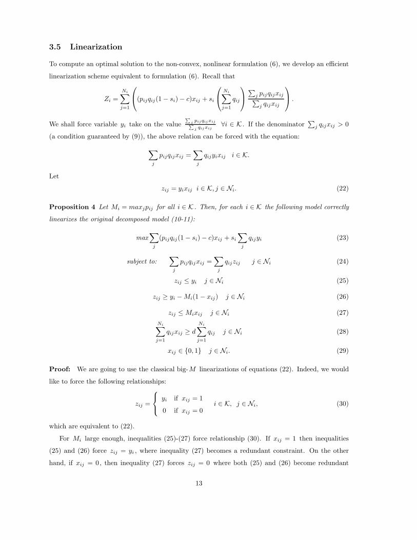
3.5 Linearization
To compute an optimal solution to the non-convex, nonlinear formulation (6), we develop an efficient
linearization scheme equivalent to formulation (6). Recall that
Zi =Ni∑j=1
⎛⎝(pijqij(1 − si) − c)xij + si
⎛⎝ Ni∑
j=1
qij
⎞⎠ ∑j pijqijxij∑
j qijxij
⎞⎠ .
We shall force variable yi take on the value∑
j pijqijxij∑j qijxij
∀i ∈ K . If the denominator∑
j qijxij > 0
(a condition guaranteed by (9)), the above relation can be forced with the equation:
∑j
pijqijxij =∑
j
qijyixij i ∈ K.
Let
zij = yixij i ∈ K, j ∈ Ni. (22)
Proposition 4 Let Mi = maxjpij for all i ∈ K . Then, for each i ∈ K the following model correctly
linearizes the original decomposed model (10-11):
max∑
j
(pijqij(1 − si) − c)xij + si
∑j
qijyi (23)
subject to:∑
j
pijqijxij =∑
j
qijzij j ∈ Ni (24)
zij ≤ yi j ∈ Ni (25)
zij ≥ yi − Mi(1 − xij) j ∈ Ni (26)
zij ≤ Mixij j ∈ Ni (27)Ni∑j=1
qijxij ≥ d
Ni∑j=1
qij j ∈ Ni (28)
xij ∈ {0, 1} j ∈ Ni. (29)
Proof: We are going to use the classical big-M linearizations of equations (22). Indeed, we would
like to force the following relationships:
zij =
⎧⎨⎩ yi if xij = 1
0 if xij = 0i ∈ K, j ∈ Ni, (30)
which are equivalent to (22).
For Mi large enough, inequalities (25)-(27) force relationship (30). If xij = 1 then inequalities
(25) and (26) force zij = yi , where inequality (27) becomes a redundant constraint. On the other
hand, if xij = 0, then inequality (27) forces zij = 0 where both (25) and (26) become redundant
13

constraints. For these linearizations to work properly Mi should be at least as large as the maximum
value each yi and consequently each zij can take. An appropriate such value for Mi is found from
the following inequality:
yi =
∑j pijqijxij∑
j qijxij≤ max
jpij
∑j qijxij∑j qijxij
= Mi.
To strengthen the linear model (23)-(29), we also added the following valid inequality for each
i ∈ K to our modelNi∑j=1
pijqijxij ≥ yid
Ni∑j=1
qij ,
which proved very effective in our numerical experiments.
4 Case Study at Two Local Chains
We developed our model upon the request of a major international FMCG conglomerate which has
significant presence in the Turkish market. The company has the largest market share in Turkey
in its core operating sectors: Fabric and Home Care products, Health and Beauty Care products,
Feminine Care products and Baby Care products. The company wanted us to provide a tool that
small and medium size supermarkets in Turkey could use to optimize the assortment on their shelves.
They believed that if the supermarkets would eliminate the unprofitable SKUs from their shelves, the
visibility of their own products, which are usually the product leaders, would increase and thereby,
their sales would be positively affected. Under such a scenario, the provided tool would assist the
creation of a win-win situation for both the supermarket and the FMCG conglomerate. They shared
their intentions with two local supermarket chains in Ankara, Turkey which in return accepted to
collaborate with us. These supermarket chains are considered as part of the “Local Chain” customer
channel that constitutes %35 of the FMCG company’s total sales volume in the country.
In this case study, we discuss the results of our model on the assortment of shampoo products
at two local chains in the Ankara region. Since these two supermarkets were only keeping monthly
sales and profitability data, our model was originally shaped around these input requirements. The
two chains agreed to disclose the requisite data for the purposes of the project. Although they stated
that they could use such a tool for different product classes, they first wanted us to demonstrate
the effectiveness of our methodology in a specific product class. We decided to focus on the shampoo
products since this product class has the maximum number of SKUs on retailers’ shelves while frequent
new product launches are still pushing the number higher. Therefore, the choice of shampoo class
14

is definitely one where efficient assortment and shelf usage is to be beneficial. Moreover, since the
FMCG company has a significant presence in this class, they agreed with this choice which could help
increase the visibility of their market leader products.
The study concentrates on two local chains, that will be referred to henceforth as “Local Chain
A” and “Local Chain B”, and on three stores of each local chain classified according to their sizes as
“small”, “medium” and “large”. The shampoo SKUs under scrutiny are classified into three categories
according to their quality levels and prices, the premium quality in category 1, the middle quality in
category 2, and low quality in category 3.
After consulting with retail managers we decided that setting the cost per period of keeping a
SKU on the shelf, parameter c in our model, to 1 local currency unit (YTL) is a reasonable choice.
We investigate the sensitivity of our results to perturbations in this value in Experiment 3 below.
A preliminary analysis of sales data according to categories, brands and store sizes yielded the
following results:
• Although some SKUs are sold in smaller quantities, they bring larger profit,
• Results change according to store size,
• There exist seasonal effects in sales; especially during the summer months noticeable increases
in sales of shampoo occur,
• There are promotions in some SKUs affecting the sales figures,
• Prices may fluctuate over months.
The local chain managers reconsider the SKUs to be carried on their shelves twice a year. As a result,
we decided to use data corresponding to six calender months each time an instance of the model is
solved. But, in order to accommodate the seasonal effects in demand, the data of each six months
period is employed to decide on the assortment of the next period corresponding to the same months
of the year (using the data with a lag of six months). This means we use the data of the previous
period corresponding to the same season for the current assortment. Average prices for SKUs were
used in our calculations to eliminate possible price fluctuations that may have occurred during the six
month period. Note that the six month period is long enough for the averages to incorporate both
promotion and regular price epochs.
It should be noted that the model we propose only deletes SKUs from the current assortment. It
does not have a feature to incorporate new SKUs that may become available in time, or old SKUs
whose popularity may rise due to new marketing efforts. In order to accommodate the situation,
we propose the chains to add the SKUs that look promising to their assortment for a period of six
15

months. After that our methodology would take care of the decision of keeping them on shelves or
delisting them.
One should also note that as the number of SKUs carried at the retailer’s shelves decreases due
to our model, the product pollution would decrease. This would allow the retailer to reorganize its
shelves in a more orderly and attractive fashion. Thus, we would actually expect this decrease to give
rise to some additional demand from visiting customers who may have been previously overwhelmed
by the sheer number of available SKUs and product pollution, and consequently left the shop without
buying any shampoo. This model does not take into account this additional demand since it cannot
be predicted based on the sales and profitability data available. This only means that under more
realistic considerations, we would eliminate even more SKUs and that the estimated profit in the
objective function would be greater.
4.1 Calculation of the substitution ratio
We observed that if a desired SKU is out of stock, a fraction of the demand for that particular SKU
will be distributed among other shampoos of the same category. This switching behavior is quantified
using a parameter s that we refer to as the substitution ratio. According to a marketing survey
commissioned upon the request of the FMCG company, a customer who cannot find his/her desired
shampoo
a. buys another brand with a probability of 0.16
b. leaves the store without buying shampoo with a probability of 0.10
c. buys the same SKU from another store with a probability of 0.53
d. buys another SKU of the same brand with a probability of 0.15
e. delays shopping with a probability of 0.06
Our main observation here is that the substitution ratio is stable within a product category. That
is to say, when a customer comes to buy a relatively cheaper product (third quality in our particular
case study) and faces an out-of-stock situation, he/she buys another product in the same category
as the one he/she was looking for. However, a customer looking for a first quality shampoo will be
less likely to switch to a lower quality shampoo when his/her preferred shampoo is not available.
Unfortunately, we have no access to data to estimate different substitution ratios for different quality
categories. Therefore, we decided to work with a single aggregate substitution ratio estimate valid for
all quality classes. This aggregate estimate was calculated as follows using the previously mentioned
marketing survey. We made the assumption that customers will keep using shampoo for hair care in
16

Store Initial d obj CPU A1 B1 C1 A2 B2 C2 A3 B3 C3 C
Size ProfitLarg
e
854.5
0.6 875.93 3.27 0.98 0.995 0.995 0.705 0.923 0.936 0.7 0.969 0.967 0.967
0.8 875.93 0.25 0.98 0.995 0.995 0.705 0.923 0.936 0.7 0.969 0.967 0.967
0.9 875.93 0.19 0.98 0.995 0.995 0.705 0.923 0.936 0.7 0.969 0.967 0.967
Mediu
m
161.4
0.6 200.92 0.84 0.455 0.727 0.768 0.449 0.689 0.706 0.452 0.802 0.814 0.754
0.8 199.13 0.76 0.545 0.808 0.838 0.536 0.801 0.796 0.452 0.802 0.814 0.814
0.9 190.96 0.5 0.682 0.909 0.92 0.681 0.901 0.888 0.645 0.903 0.906 0.903
Sm
all
138.3
0.6 189.27 0.98 0.52 0.749 0.765 0.376 0.602 0.651 0.276 0.639 0.648 0.699
0.8 180.11 0.34 0.58 0.8 0.811 0.576 0.801 0.827 0.517 0.81 0.818 0.819
0.9 169.39 0.39 0.72 0.91 0.904 0.718 0.9 0.911 0.69 0.906 0.907 0.907
Table 1: Results for Local Chain A Stores
Store Initial d obj CPU A1 B1 C1 A2 B2 C2 A3 B3 C3 C
Size Profit
Larg
e
1169.8
0.6 1200.67 0.327 0.941 0.992 0.992 0.742 0.961 0.98 0.528 0.77 0.786 0.975
0.8 1200.48 0.22 0.941 0.992 0.992 0.742 0.961 0.98 0.583 0.815 0.831 0.978
0.9 1198.73 0.15 0.941 0.992 0.992 0.742 0.961 0.98 0.694 0.901 0.902 0.981
Mediu
m
578.4
0.6 600.44 0.17 0.978 0.996 1 0.836 0.957 0.994 0.806 0.961 0.970 0.99
0.8 600.44 0.16 0.978 0.996 1 0.836 0.957 0.994 0.806 0.961 0.970 0.99
0.9 600.44 0.08 0.978 0.996 1 0.836 0.957 0.994 0.806 0.961 0.970 0.99
Sm
all
58.8
0.6 108.75 0.94 0.395 0.606 0.626 0.352 0.603 0.643 0.441 0.617 0.616 0.63
0.8 98.28 0.36 0.581 0.801 0.808 0.563 0.801 0.819 0.647 0.802 0.804 0.811
0.9 88.88 0.19 0.698 0.9 0.904 0.718 0.9 0.916 0.794 0.91 0.911 0.911
Table 2: Results for Local Chain B stores
the long run, and those customers “buying nothing” in the group b. above will come back to the same
store with a 0.5 probability. Adding to this figure, the probabilities from a, d and e groups above, we
obtain the estimate 0.42 for s used in the rest of this study. We also provide numerical results below
for the sensitivity of our findings to the particular value of the substitution ratio.
4.2 Results
We used GAMS/CPLEX 10 system to solve the linear optimization model introduced in Subsection
3.5 to optimality for each of the three stores of Local Chain A and those of Local Chain B. We
summarize below our results in three experiments.
Experiment 1: The impact of the minimum conservation ratio. In Tables 1 and 2 below
we report the results of our computational experiments for both Local Chain A and Local Chain B,
respectively, with the substitution ratio s and cost parameter c fixed, under three different values
17

of the minimum conservation ratio d , namely 0.6, 0.8 and 0.9. The first column under the heading
“initial profit” gives the initial total estimated profits using the data made available for this study.
Under the column “obj” we report the total estimated profit figure after elimination. The column
“cpu” gives the solution time of the linearized model in seconds. The quantities Ai, Bi, Ci , i = 1, 2, 3
and C are defined as follows:
Ai =
∑j xij
Ni, Bi =
∑j qijxij∑
j qij, Ci =
∑j pijqijxij∑
j pijqij, and, C =
∑ij pijqijxij∑
ij pijqij.
The quantity Ai represents the ratio of the number of SKUs kept on the shelf after elimination to
the total number of SKUs initially on shelf in category i (SKU retained ratio). Similarly, we use Bi
to denote the ratio of sales volume from the SKUs kept on the shelf to the total sales volume initially
in category i (volume retained ratio). In Ci we record the ratio of the profit due to the SKUs kept
on the shelf to the total profit initially from category i (value retained ratio). Finally, C is used to
quantify the total profit ratio across all categories (overall value retained ratio).
The reader should note that d imposes a lower bound on the volume retained ratio at each category
(Bi ). For the Local Chain A Large Store, the value of d does not affect the results. In the Local Chain
A Medium and Small stores, we observe –based on Ai values– decreases in the eliminated SKUs in all
categories by an approximately equal factor as the minimum conservation ratio increases. In a more
stringent elimination effort (lower values of d) larger number of SKUs from lower quality categories
are removed compared to the premium category. This result agrees with the intuition that higher
quality, higher price SKUs resist elimination better than lower quality, lower price ones since the
former have potentially a larger contribution to the total profitability of the store. In the Local Chain
B’s Large and Medium stores the minimum conservation ratio d has little or no effect on elimination.
In cases the model suggests a considerable elimination when it is not tightly constrained by d (when
d = 0.6), the number of eliminated SKUs significantly decreases as d increases. In the Small store, a
more discernible elimination takes place in all categories while it is slightly more pronounced in the
middle category.
We observe that the model advocates a sizable elimination in the Small stores, an indication of
poor shelf management practices in these stores. The local chains seem to have a tendency to cram too
many SKUs even when the space or demand patterns do not justify it. It seems advisable that smaller
stores get a handle on profitability increases by keeping a reduced assortment where the reduction
should be more severe in the lower quality and lower price categories. In other words, avoiding product
pollution seems to be particularly beneficial for smaller stores. This observation is also supported by
a more marked profit increase due to elimination in the smaller stores.
It is interesting that the optimal solution of the model suggests that there is a consistent ascendant
18

0,75
0,8
0,85
0,9
0,95
1
0 0,5 1 1,5 2
c
Ret
ain
ed S
KU
Rat
io
d=0.6
d=0.8
d=0.9
Figure 1: Overall SKU retained ratio versus c
ordering in the SKUs retained, volume retained and value retained at each category. The model tries
to keep the SKUs that contribute a larger share of the original profit while performing elimination. In
order to achieve this, it has to conserve SKUs contributing more to the sales volume as well –although
to a lesser extent–, since sales volume is one of the two determinants of profit along with the price.
The SKUs retained trails the previous two measures, since in order to maximize profit one has to keep
a certain number of SKUs, but eliminate SKUs with limited contribution to the profit.
Experiment 2: The impact of c . In Figures 1 to 2 we illustrate the impact of the cost parameter
c on the elimination of SKUs. We select Local Chain A Large store as our test store. In Figure 1 we
report the overall SKU retained ratios (∑
ij xij∑i Ni
) achieved by the results of our model at different values
of minimum conservation ratios and increasing c from 0 to 2 in steps of 0.1. As expected, the larger
values of c , the cost of keeping SKUs on the shelf, lead to increased elimination patterns. In Figure
2 we report SKU retained ratio in all three categories for the value of d fixed to 0.8. Interestingly,
the middle category SKUs seem to be more susceptible to sharper elimination as c increases than the
other categories. Apparently, the model sheds more SKUs from the middle category than from the
extreme categories as the cost of keeping SKUs on the shelf goes up. Similar observations are made
when the value of d is 0.6 or 0.9.
Experiment 3: The impact of s . While we adopted the value of s = 0.42 in our previous
experiments, we tested the sensitivity of the results to different values of s ranging from 0.35 to
0.5 using the Local Chain A Large store for illustration. Figure 3 summarizes the results of this
19

0,75
0,8
0,85
0,9
0,95
1
0 0,5 1 1,5 2
c
Ret
ain
ed S
KU
Rat
io (
d=0
.8)
Category 1
Category2
Category 3
Figure 2: SKU retained ratio for all three categories versus c at d = 0.8
0,80,820,840,860,880,9
0,920,940,960,98
1
0,35 0,4 0,45 0,5
s
Ret
ain
ed S
KU
Rat
io (
d=0
.8)
Category 1
Category 2
Category 3
Figure 3: Retained SKU ratio versus s at d = 0.8
20

873874875876877878879880881882
0,35 0,4 0,45 0,5
s
Op
tim
al P
rofi
t
d=0.6, 0.8
d=0.9
Figure 4: Optimal objective function value versus s
experiment at d = 0.8. An observation similar to that made in Experiment 2 prevails here. The
middle category SKUs are clearly more sensitive to perturbations in the substitution ratio s than the
extreme categories. The changing values of s do not seem to affect much the high quality and low
quality categories. This reflects the existence of an abundance of SKUs exhibiting a wide spectrum
of profitability profile, which responds to increases in the substitution ratio by gradually enlarging
the set of delisted SKUs. It is to be expected that the low quality category does not respond to
increased substitution ratio, since the range of prices –and thereby profitability– is rather limited in
this category and that does not create an opportunity for capturing profit by substitution. Similar
observations are made when the value of d is 0.6 or 0.9.
The impact of the substitution ratio on the optimal objective function value for different values of
d in Figure 4 indicates a convex increasing curve. Higher substitution ratios increase total profit faster
than the corresponding increase in substitution. This impact is less pronounced at higher minimum
conservation ratios, i.e., less severe elimination, as expected.
5 Conclusion
In this paper we developed a practical optimization model that improves the product mix on the
shelves of a retailer, and thus reduces product pollution. We applied the proposed model to two local
supermarket chains using proprietary data disclosed to us by the chain managers. This project was
undertaken upon the request of an FMCG conglomerate that supplies these –as well as others– retail
channels. Their motivation to initiate such an endeavor was to persuade the local supermarket chains
21
that a limited assortment would benefit their profitability, while simultaneously solving the visibility
problems faced by the market leader products of the FMCG company. To continuously guide the chain
manager on the correct assortment, they were asking for a simple and practical tool. We developed
such a tool based on the model presented in this paper. To demonstrate the usefulness of our tool, we
decided to first focus on the highly problematic shampoo class. Our results that were summarized in
Section 4 revealed that a judicious elimination based on our model has the potential for a significant
increase in profitability. The FMCG company as well as the studied supermarket management are in
the process of incorporating this decision support tool into their operations.
References
[1] Cachon, G.P., C. Terwiesch, Y. Xu. 2005. Retail assortment planning in the presence of consumer
search. Manufacturing Service Operations Mgmt. 7 (4) 330–346.
[2] Corstjens, M., P. Doyle. 1981. A model for optimizing retail space allocations. Management
Science. 27 822–833.
[3] Kok, A.G., M.L. Fisher. 2006. Demand estimation and assortment optimization under substitu-
tion: Methodology and application. To appear in Operations Research.
[4] Kok, A.G., M.L. Fisher, R. Vaidyanathan. 2005. Retail assortment planning: review of liter-
ature and industry practice. To appear in N. Agrawal, S. Smith. (eds.). Retail Supply Chain
Management. Kluwer, Amsterdam.
[5] Mahajan, S., van Ryzin, G.J. 1998. Retail Inventories and Consumer Choice. Tayur, S. et al.
(eds.). Quantitative Methods in Supply Chain Management. Kluwer, Amsterdam.
[6] Mahajan, S., G. van Ryzin. 2001. Stocking retail assortments under dynamic consumer substitu-
tion. Operations Research. 49 334–351.
[7] Netessine, S., N. Rudi. 2003. Centralized and competitive inventory models with demand substi-
tution. Operations Research. 51. 329–335.
[8] Schaible, S. 1977. A note on the sum of a linear and linear-fractional function. Naval Research
Logistics Quarterly. 24. 691–693.
[9] Smith, S.A., N. Agrawal. 2000. Management of multi-item retail inventory systems with demand
substitution. Operations Research. 48 50–64.
22

[10] Urban, T.L. 1998. An inventory-theoretic approach to product assortment and shelf space allo-
cation. Journal of Retailing. 74 15–35.
[11] van Ryzin, G., S. Mahajan. 1999. On the relationship between inventory costs and variety benefits
in retail assortments. Management Science. 45 1496–1509.
23