J. theor. Biol. (1996) 178, 29–43

0022–5193/96/010029+15 $12.00/0 7 1996 Academic Press Limited

A Model for Wolf-Pack Territory Formation and Maintenance

K. A. J. W,†‡ M. A. L§ J. D. M

Department of Applied Mathematics, University of Washington, Seattle, WA 98195, U.S.A.

(Received on 31 March 1995, Accepted on 14 August 1995)

A model is developed to investigate the formation and maintenance of wolf territories based on thespatial patterns observed in northeastern Minnesota. Initially we simplify the model to consider themovements of a single pack. In this case we obtain steady state density distributions corresponding toterritories and determine how the size of a territory depends on the number of wolves in a pack. Wesuggest how, with sufficient access to the relevant field data, this simplified model could be used toestimate some of the model parameters. The complete multi-pack model shows how interactionsbetween adjacent packs determine the shape of the territory. We investigate the solutions to themathematical model systems and discuss ecological implications.

7 1996 Academic Press Limited

1 Introduction

Territorial behaviour is an intrinsic part of theecology of many mammals and introduces large scalespatial heterogeneity into population interactions.Clearly such heterogeneity can have major effects onthe spread of disease and population survival, butdespite this there have been very few attempts tomodel the phenomenon mathematically.

In 1939, Noble defined territory as ‘‘any defendedarea’’, thus providing a very general and flexibledefinition for future development. Since then therehas been a large number of alternative definitionseach with a slightly different emphasis. Emlen (1957)suggested ‘‘a space within which an animal isaggressive to and usually dominant over certainintruders’’, Pitelka (1959) suggested ‘‘any exclusivearea’’, Eibl-Ebesfeldt (1970) ‘‘a space associatedintolerance’’ and Brown & Orians (1970) ‘‘a fixedexclusive area with the presence of defense that keepsrivals out’’. In all cases the territory is an activelydefended fixed area in space (but this can vary over

time) and the holder has exclusive use of the spacewith respect to a certain group of individuals. It isimportant to reiterate that boundary areas canoverlap temporally, allowing them to be used by twodifferent groups at different times (Brown & Orians,1970). The large number of definitions that have beendeveloped by field ecologists indicates the importanceof territoriality in many different natural systems.

The motivation for this paper came from fieldstudies on the ecology of the timber wolf (Canis lupis)carried out in northeastern Minnesota over a periodof many years (see, for example Mech, 1977a; vanBallenberghe et al., 1975). Although wolves are highlydeveloped carnivores with a complex social structure,we restrict discussion of wolf behaviour in this paperto those elements most directly related to territorial-ity.

Wolf packs are extended family groups typicallyconsisting of 3–12 wolves with territories rangingfrom 125–310 km2 in northeastern Minnesota (vanBallenberghe et al., 1975). Buffer zones whichseparate adjacent territories can be as wide as 1–2 kmcovering between 25 and 40% of the available land(Mech 1977b, c). These buffer regions are areas ofpotential inter-pack conflict into which wolves rarelytrespass, although when prey levels are low within theterritory cores, wolves may move into the buffer zones

† Current address: Department of Zoology, Downing Street,University of Cambridge, Cambridge, CB2 3EJ, UK.

‡ Corresponding author.§ Current address: Department of Mathematics, University of

Utah, Salt Lake City, UT 84112, USA.

29

. . . .30

to hunt and the levels of inter-pack strife can increase(Mech, 1977b).

One pair of wolves, known as the alpha couple,dominate pack activities. This alpha couple is usuallythe only pair to produce young. Pups are born in thelate spring, are reared at the den site for some timeafter birth, and then move to above groundrendezvous sites. Thus, during the summer monthspack activity is centred around the den or rendezvoussites where the pups are fed and cared for. By the endof the summer, the pups have developed sufficientlyand are able to move with the pack. In this way, theden loses its focus and the pack can move extensivelythrough the territory.

Olfactory stimuli are well known to be used in avariety of different roles by many mammals. Theraised leg urination (RLU) is closely connected withterritorial marking and maintenance (Peters & Mech,1975). These markings are made throughout theterritory along wolf trails but, more importantly, theyincrease significantly around the territory edges givingrise to high concentrations of RLU markings from allpacks in the buffer regions. Unlike other olfactorystimuli associated with wolves, the RLU shows littlecorrelation with pack size. In fact, it is the alpha pairwhich is predominantly responsible for this marking.

Mathematical models describing animal movementhave been proposed, for example, by Skellam (1951)in which the idea of modelling animal movement withsimple Fickian diffusion was developed. Okubo(1986) investigated mathematical models describinganimal groups such as schools and swarms whilemore recently, Grunbaum & Okubo (1993) reviewedmodels for social aggregations.

The specific issue of territoriality, however, hasbeen less often considered. Statistical models, both ofthe univariate and bivariate type were compared byvan Winkle (1976) for their ability to predict homerange movements. A home range is similar to aterritory but there is no element of defense associatedwith this area so models of home range activityare of limited value when describing territorialbehaviours and movements. Don & Renolls (1983)used a more sophisticated model based uponprobability distributions to determine home rangemovement when attraction points were used torepresent a nesting or similar site. Benhamou (1989)developed a correlated random walk model todescribe animal movement which is governed byolfactory gradients and produced results in agreementwith field studies. A probability model concernedspecifically with territorial animals was proposed byBacon et al. (1991) to investigate the resourcedispersion hypothesis of Macdonald (1983) which

suggests that spatial distribution of resourcesdetermines territory size and the richness of theseresources independently determines group size. Theyuse normal distribution to represent yield from aterritory during a feeding period for a habitat ofdiscrete independent food patches. The results showagreement with Macdonald’s theory (1983). Moregenerally, Covich (1976) investigated the shape andsize of foraging areas using graphical techniques.These simple, non-mechanistic models give anindication of the dependence of foraging areas onecological constraints such as predation, resourcedistribution and population density. Another simplemodel by Possingham & Houston (1990) reconsidersthe ‘‘marginal value theorem’’ (Charnov, 1976) in thecase of territorial foragers and shows that resourcerenewal is an important element of foraging strategyfor a territorial animal.

Of particular relevance to this paper, Taylor &Pekins (1991) used a modified Lokta-Volterra systemof ordinary differential equations to investigate howimportant the buffer zone is in maintaining thestability of the wolf-deer ecosystem in Minnesota.Here, however, territories were specified as hexagonalshapes and movement between the core and bufferwas achieved by splitting the deer population into twosubpopulations. As the spatial structure of territory isassigned, nothing can be deduced from this modelabout the natural development and maintenance ofwolf territories.

The recent paper by Lewis & Murray (1993)considers a partial differential equation model withtwo wolf packs and deer and shows how the systemgives rise to territorial patterns and the subsequentspatial segregation of wolves and their prey, thewhite-tailed deer (Odocoileus virginianus). This modelhas a similar structure to that described below,incorporating dispersive movement to represent wolfforaging activities and a convective term representingmovement towards an organising centre. The modeldescribed here, however, differs from that one inseveral ways. In the Lewis & Murray model,convection back towards an organising centre occursonly upon encountering foreign RLU markings. Inour model, this component of movement occursirrespective of any olfactory stimuli and we representwolf response to friendly and foreign RLUs withchemotactic type terms.

This paper considers territory formation withoutpredator–prey interactions. Subsequent papers willdeal with this aspect (White et al., submitted). Ourprimary interest is in summer movement patternswhen the den is a focal point of pack activity and thuswe are essentially considering a model with a time

31

span of several months. We begin by formulatingthe mathematical model assuming that there aretwo wolf packs in a region with plentiful foodsupply. Analysis is carried out on the simplersingle pack model and shows that territories canbe formed even in the absence of neighbours.The steady state solution for the single pack modelallows us to determine a relation between pack andterritory size. The interaction of several packs isshown to introduce spatial heterogeneities into thewolf density distributions about the den location andallows an investigation of RLU density distributionin relation to the wolf density distribution. We alsodiscuss model solutions when the den is no longera focus of activity in the winter months and showthat, in its present form, the model is rather limitedin its ability to describe the density distributions inthis case.

2 Model Formulation

The behaviour and ecology of the wolf are clearlyhighly complex but the stability of the territoriesfound in N.E. Minnesota suggest that there arecertain mechanisms underlying the movement of thepack members.

To define state variables, we must account for thesize of the territory relative to the pack size. As wolfpacks are small in size when compared with theirterritory sizes, there will be large periods of time whenno wolf is found in a given location. In view of this,we define the state variables as expected density ofwolves using a probabilistic approach. Scent markingis thought to be an important component inmaintaining territories—we reflect this in the modelby assigning two state variables to each wolf pack,one for expected wolf density and the other forexpected RLU density. In this case the state variablesfor a two pack model are:

u(x, t)=expected density of scent marking wolvesin pack 1

v(x, t)=expected density of scent marking wolvesin pack 2

p(x, t)=expected density of RLUs from pack 1q(x, t)=expected density of RLUs from pack 2.In this simplified model system, wolf movement

is assumed to comprise four components—movementtowards the den (during summer) to feed the pups,dispersal to find food and to mark the territory,movement away from regions of foreign RLUmarking and movement back towards familiarRLU marking. We assume that there is no starvationor inter-pack conflict during the summer monthsand hence that there is no wolf mortality. For the

adult members of a pack at least, this is not anunreasonable assumption (Mech, 1970).

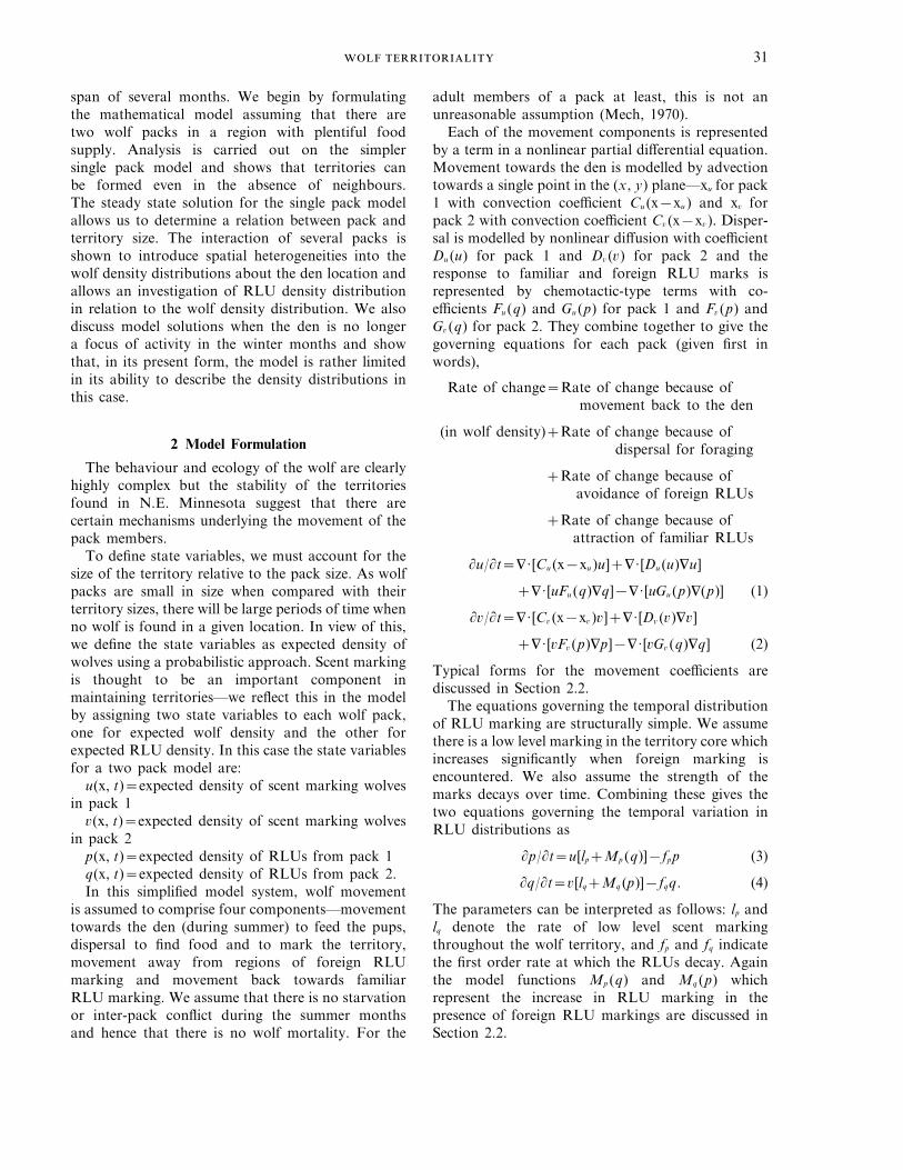
Each of the movement components is representedby a term in a nonlinear partial differential equation.Movement towards the den is modelled by advectiontowards a single point in the (x, y) plane—xu for pack1 with convection coefficient Cu (x−xu ) and xv forpack 2 with convection coefficient Cv (x−xv ). Disper-sal is modelled by nonlinear diffusion with coefficientDu (u) for pack 1 and Dv (v) for pack 2 and theresponse to familiar and foreign RLU marks isrepresented by chemotactic-type terms with co-efficients Fu (q) and Gu (p) for pack 1 and Fv (p) andGv (q) for pack 2. They combine together to give thegoverning equations for each pack (given first inwords),

Rate of change=Rate of change because ofmovement back to the den

(in wolf density)+Rate of change because ofdispersal for foraging

+Rate of change because ofavoidance of foreign RLUs

+Rate of change because ofattraction of familiar RLUs

1u/1t=9·[Cu (x−xu )u]+9·[Du (u)9u]

+9·[uFu (q)9q]−9·[uGu (p)9(p)] (1)

1v/1t=9·[Cv (x−xv )v]+9·[Dv (v)9v]

+9·[vFv (p)9p]−9·[vGv (q)9q] (2)

Typical forms for the movement coefficients arediscussed in Section 2.2.

The equations governing the temporal distributionof RLU marking are structurally simple. We assumethere is a low level marking in the territory core whichincreases significantly when foreign marking isencountered. We also assume the strength of themarks decays over time. Combining these gives thetwo equations governing the temporal variation inRLU distributions as

1p/1t=u[lp+Mp (q)]−fpp (3)

1q/1t=v[lq+Mq (p)]−fqq. (4)

The parameters can be interpreted as follows: lp andlq denote the rate of low level scent markingthroughout the wolf territory, and fp and fq indicatethe first order rate at which the RLUs decay. Againthe model functions Mp (q) and Mq (p) whichrepresent the increase in RLU marking in thepresence of foreign RLU markings are discussed inSection 2.2.

. . . .32

To completely specify the problem mathematically,we give the initial expected density distributions,

u(x, 0)=hu (x), p(x, 0)=hp (x),

v(x, 0)=hv (x), q(x, 0)=hq (x) (5)

for arbitrary functions hu (x), hp (x), hv (x), and hq (x).Typically we set hp (x)=hq (x)=0 because we areprimarily interested here in initial territory formation.

We consider the problem on some domain V withzero flux boundary conditions for the expected wolfdensity distributions; that is,

0=[Cu (x−xu )u+Du (u)9u+uFu (q)9q−

uGu (p)9(p)]·n on 1V

0=[Cv (x−xv )v+Dv (v)9v+vFv (p)9p−

vGv (q)9(q)]·n on 1V (6)

where n is the outward normal to the domain on itsboundry 1V. The zero flux boundary conditioneffectively imposes the biological constraint that thereis no immigration or emigration of wolves across theboundary of the finite study area.

Equations (1) and (2) with the boundary conditionsgiven in (6) are conservation equations and thus thenumber of wolves in a pack remains constant for alltime. To show this we look at just one of theequations, (1) for example, and suppose that thenumber of wolves in the pack is Qu (t) where

Qu (t)=gV

u(x, t)dx. (7)

Using (1), (6), (7) and the divergence theorem, we get

1Q1t

=gV

1u1t

dx

=gV

9·[Cu (x−xu )u+Du (u)9u+uFu (q)9q

−uGu (p)9(p)] dx

=g1V

[Cu (x−xu )u+Du (u)9u+uFu (q)9q

−uGu (p)9p]·dn

=0 (8)

Thus the number of wolves in the pack does notchange with time; that is

Qu (t)=Qu (0)=Qu=constant.

Similarly for pack 2,

Qv (t)=Qv (0)=Qv=constant.

2.1. -

We non-dimensionalize the model system to allowcomparison between the relative size of modelparameters and to reduce the number of parametersin the problem. The area of V is given by

A=gV

dx

and we define L=A1/m where m is the dimension of thesolution domain (that is, m=1 for 1 space dimensionand m=2 for 2 space dimensions). We use the decaytime for the RLUs of pack 1 as a typical timescale.We take U0 and V0 to be average expected wolfdensities for the respective packs, that is

U0=Qu

Lm V0=Qv

Lm

and non-dimensionalize by letting

u*=uU0

, v*=vV0

, p*=fp

U0lpp,

q*=fp

V0lqq, t*=tfp , x*=

xL

C*u =Cu

Lfp, C*v =

Cv

Lfp, D*u =

Du

L2fp, D*v =

Dv

Lfp

F*u =FuV0lqL2f 2

p, F*v =

FvU0lpL2f 2

p,

G*u =GuU0lpL2f 2

p, G*v =

GvV0lqL2f 2

p

M*p =Mp

lp, M*q =

Mq

lq, f=

fq

fp.

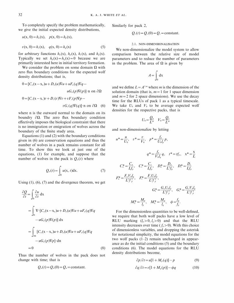
For the dimensionless quantities to be well-defined,we require that both wolf packs have a low level ofRLU marking (lpq0, lqq0) and that the RLUintensity decreases over time ( fpq0). With this choiceof dimensionless variables, and dropping the asteriskfor notational simplicity, the model equations for thetwo wolf packs (1–2) remain unchanged in appear-ance as do the initial conditions (5) and the boundaryconditions (6). The model equations for the RLUdensity distributions become,

1p/1t=u[1+Mp (q)]−p (9)

1q/1t=v[1+Mq (p)]−fq (10)

33

The conservation condition (7) now takes the form

gV

u(x, t) dx=1 gV

v(x, t) dx=1, (11)

and the dimensionless domain for study is an area orlength equal to unity. The integral relation (11) showsthat we can consider the dimensionless dependentvariables u(x, t), v(x, t) as probability densityfunctions for the location of the wolves at some timet. We use the non-dimensional form of the system inthe analysis below to indicate which parameters areimportant in determining the qualitative behaviour ofthe solution.

2.2.

Okubo (1980) used the advection-diffusionequation

1u1t

=1

1x 0Cu (x)u+Du (u)1u1x1

to describe the swarming of the insects. In thatone-dimensional model he used a density dependentdiffusion coefficient of the form

Du (u)=duun

for some positive value of n and the functionCu (x−xu ) was chosen as the piecewise discontinuousfunction

cu sgn(x−xu ).

It can be seen that this model is one that wouldgovern the movements of a pack (in one spacedimension) if their movements were unaffected byRLU markings for a general Cu (x−xu ). We use thesefunctional forms as a basis, therefore, for the modelfunctions Du (u), Cu (x−xu ) proposed here.

In particular, we use an identical diffusioncoefficient chosen to have a non-negative exponent nand compare the cases n=0 and nq0 for which thesolution takes different forms. The first caserepresents standard Fickian diffusion so that, in theabsence of the advection term, the wolves move in arandom way during their foraging activities. Theother represents density dependent diffusion wherethe rate of random motion, as measured by thediffusion coefficient Du , is highest in those regions thatare used most commonly (u high) and lowest in thoseregions which are used least (u low). In fact, it isassumed that as a wolf approaches totally unfamiliarregions (u 4 0) the rate of random motion ap-proaches zero (Du 4 0). In effect this means that if webegin with a density distribution which is not spatially

homogeneous in V, (for example a hat or deltafunction) the leading edge moves outwards with afinite speed. While recognising that this nonlineardiffusion term has not been derived directly from theunderlying stochastic process [see, for example,discussion of the Fokker Planck equation in Okubo(1980)], we believe that this term provides an effectivemeans for characterizing movement rates based onfamiliarity with a region. As this work is the first ofits kind to mathematically investigate the movementsof territorial carnivores such as wolves using partialdifferential equations, we have chosen to comparethese situations and see what information each canprovide.

The convective flux term of the Okubo (1980)model is generalized to a two-dimensional function ofthe form

Cu (x)=cu tanh (br)xr

(12)

where r=>x> is the distance of a point from theden site.

This formation differs from that of Okubo in thatCu (x) is a continuous function of space. Theparameter cu measures the maximum speed of the wolfwhen moving towards the den and b measures thechange in the rate of convective movement as the denis approached. In particular we can see that the abovefunction in one space dimension approaches that ofOkubo (1980) as b 4a. In summer when the den isa focus of activity we take cuq0 and in winter whenthe den has been abandoned we can set cu=0.

We assume that when there is no RLU marking ata location, there is no wolf taxis away from foreignor towards familiar RLUs. Moreover, we assume thatthere is a maximum value for this coefficient whichcorresponds to the maximum wolf speed. Wetherefore take Fu (q), Fv (p), Gu (p) and Gv (q) to bemonotonic non-decreasing functions with Fu (0)=0,Fv (0)=0, Gu (0)=0, Gv (0)=0 which asymptote to afinite non-zero value.

Finally, the functions Mp (q) and Mq (p) determinethe extent to which RLU marking increases in thepresence of foreign scent marks. They are alsobounded monotonically non-decreasing functionssimilar in form to Fu (q), Fv (p), Gu (p), Gv (q).Qualitative forms for these functions are shown inFigs 1–2.

3. Single Pack Steady-State Distribution

If we suppose that pack 1, for example, is notaffected by the presence of RLU marks (eitherfamiliar or foreign) so that Fu (q)=Gu (p)=0, we can

. . . .34

determine the steady-state solution for this packanalytically. This situation corresponds to the idea ofhome range because there is no mechanism of defenceinvolved in the pack activities. Moreover, when thedimensionless distributions are converted back intotheir dimensional form, we can determine arelationship between pack and territory (home range)size.

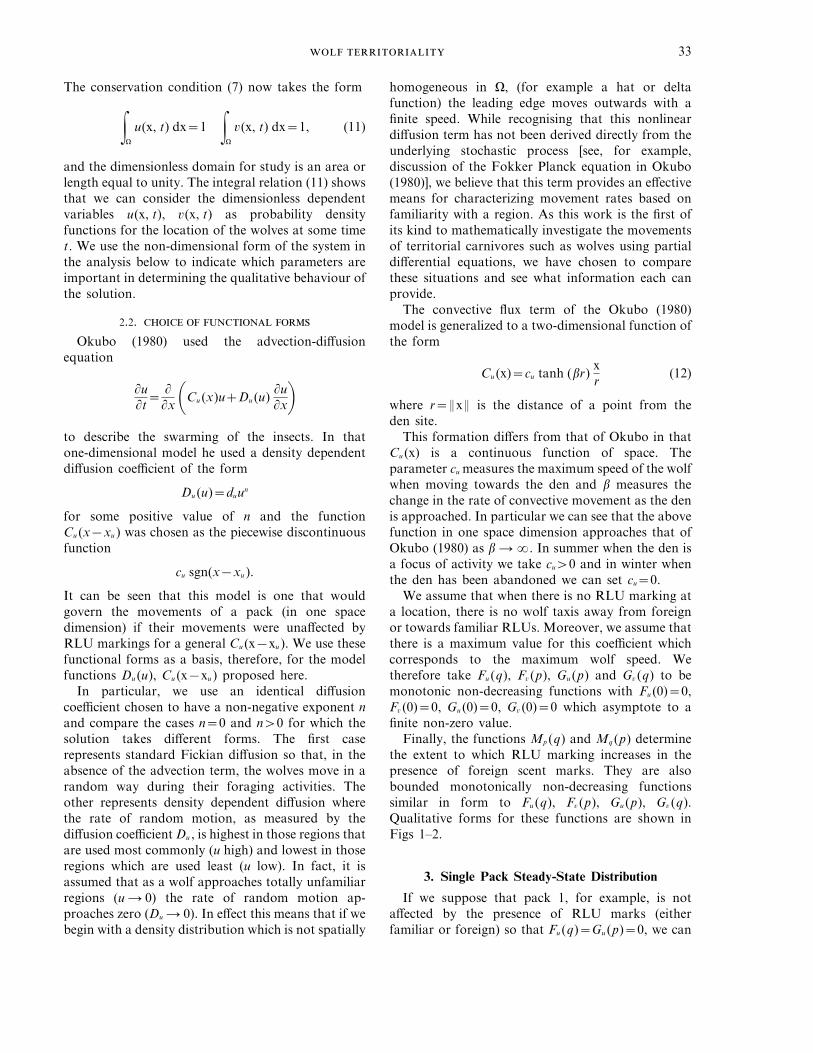
A steady state arises when the diffusive fluxbalances the convective flux so that 1u/1t=0. In onespace dimension the dimensionless convective flux(12) simplifies to

Cu (x−xu )=cu tanh [b(x−xu )]

and the non-dimensional steady state wolfdistribution is governed by (1) with 1u/1t=0;that is

1

1x 0cu tanh [b(x−xu )]u+duun 1u1x1=0. (13)

We can integrate this once and apply the zero fluxboundary condition to obtain

cu tanh (b(x−xu ))+duun 1u1x

=0 (14)

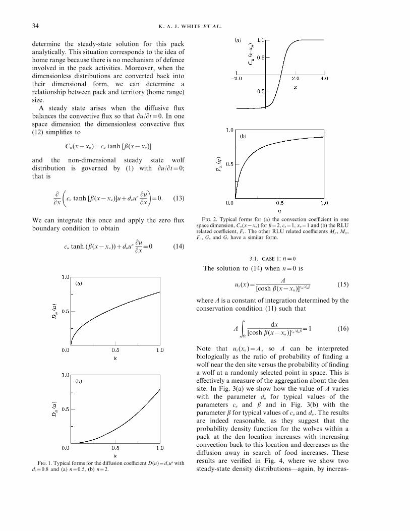
F. 2. Typical forms for (a) the convection coefficient in onespace dimension, Cu (x−xu ) for b=2, cu=1, xu=1 and (b) the RLUrelated coefficient, Fu . The other RLU related coefficients Mp , Mq ,Fv , Gu and Gv have a similar form.

3.1. 1: n=0

The solution to (14) when n=0 is

us (x)=A

[cosh b(x−xu )]cu /dub (15)

where A is a constant of integration determined by theconservation condition (11) such that

A gV

dx[cosh b(x−xu )]cu /dub=1 (16)

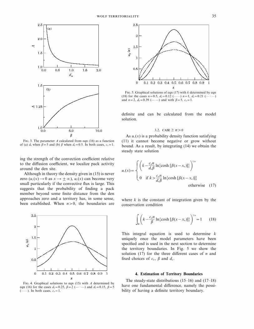
Note that us (xu )=A, so A can be interpretedbiologically as the ratio of probability of finding awolf near the den site versus the probability of findinga wolf at a randomly selected point in space. This iseffectively a measure of the aggregation about the densite. In Fig. 3(a) we show how the value of A varieswith the parameter du for typical values of theparameters cu and b and in Fig. 3(b) with theparameter b for typical values of cu and du . The resultsare indeed reasonable, as they suggest that theprobability density function for the wolves within apack at the den location increases with increasingconvection back to this location and decreases as thediffusion away in search of food increases. Theseresults are verified in Fig. 4, where we show twosteady-state density distributions—again, by increas-

F. 1. Typical forms for the diffusion coefficient D(u)=duun withdu=0.8 and (a) n=0.5, (b) n=2.

35

F. 3. The parameter A calculated from eqn (16) as a functionof (a) du when b=5 and (b) b when du=0.5. In both cases, cu=1.

F. 5. Graphical solutions of eqn (17) with k determined by eqn(18) for the cases n=0.5, du=0.12 (——) n=1, du=0.21 (— · —)and n=2, du=0.39 (— —) and with b=5, cu=1.

definite and can be calculated from the modelsolution.

3.2. 2: nq0

As us (x) is a probability density function satisfying(11) it cannot become negative or grow withoutbound. As a result, by integrating (14) we obtain thesteady state solution

us (x)=gG

G

F

f

0k−cundub

ln{cosh [b(x−xu )]}11/n

0 if kqcundub

ln{cosh [b(x−xu )]}

otherwise (17)

where k is the constant of integration given by theconservation condition

gV 0k−cunb

ln{cosh [b(x−xu )]}11/n

=1 (18)

This integral equation is used to determine kuniquely once the model parameters have beenspecified and is used in the next section to determinethe territory boundaries. In Fig. 5 we show thesolution (17) for the three different cases of n andfixed choices of cu , b and du .

4. Estimation of Territory Boundaries

The steady-state distributions (15–16) and (17–18)have one fundamental difference, namely the possi-bility of having a definite territory boundary.

ing the strength of the convection coefficient relativeto the diffusion coefficient, we localize pack activityaround the den site.

Although in theory the density given in (15) is neverzero (us (x)4 0 as x 42a), us (x) can become verysmall particularly if the convective flux is large. Thissuggests that the probability of finding a packmember beyond some finite distance from the denapproaches zero and a territory has, in some sense,been established. When nq0, the boundaries are

F. 4. Graphical solutions to eqn (15) with A determined byeqn (16) for the cases du=0.25, b=2 (— · —) and du=0.15, b=5(——). In both cases, cu=1.

. . . .36

4.1. 1: n=0

In the first case where we are using ordinaryFickian diffusion, us (x)=0 only when x=2a. Thereis no definite region in space beyond which theprobability of spotting a wolf from the pack is zeroalthough this probability becomes immeasurablysmall at large distances from the den. The spatialheterogeneity that arises in the solution demonstratesa form of territoriality and, if we assume somethreshold density within which there is an 80%chance of finding an individual, then we obtainterritories with n=0. When there is no den, however,the territory breaks down completely as we show inSection 8.1.

4.2. 2: n$0

When n is non-zero, the density distributionbecomes zero at a finite distance from the den. Nowus (x)=0 when k=n/dub ln{cos h[b(x−xu )]}. If thisoccurs at x=xu2xb then xb can be determineduniquely by

k=cundub

ln[cosh (bxb )], xbq0,

[see eqn (17)]. The spatial points xu2xb define thelimits of the wolf territory. Figure 5 shows thatthere is a difference in the shape of the leading edgebetween the cases 0QnQ1, n=1 and nq1 and thisarises in the gradient of the system. Rearranging (14)we have

1u1x

=−tanh [b(x−xu )]u1−n.

At the leading edge, u=0 so that if 0QnQ1,1u/1x=0, if n=1, 1u/1x=−tanh [b(xb−xu )] and ifnq1, 1u/1x=a. Ecologically this distinguishes thecases where there is a gradual or an abrupt end to theterritory. In all cases, the result is a non-dimensionalsteady state expected wolf density distribution givenby (17) as

us (x)=gG

G

F

f

$cundub

ln 0 cosh bxb

cosh b(x−xu )1%1/n

0

=x−xu =Exb

otherwise.

(19)

This non-negative function of x satisfies the boundaryconditions. Moreover we can see that the steady statehas boundaries at a fixed and finite distance from theden.

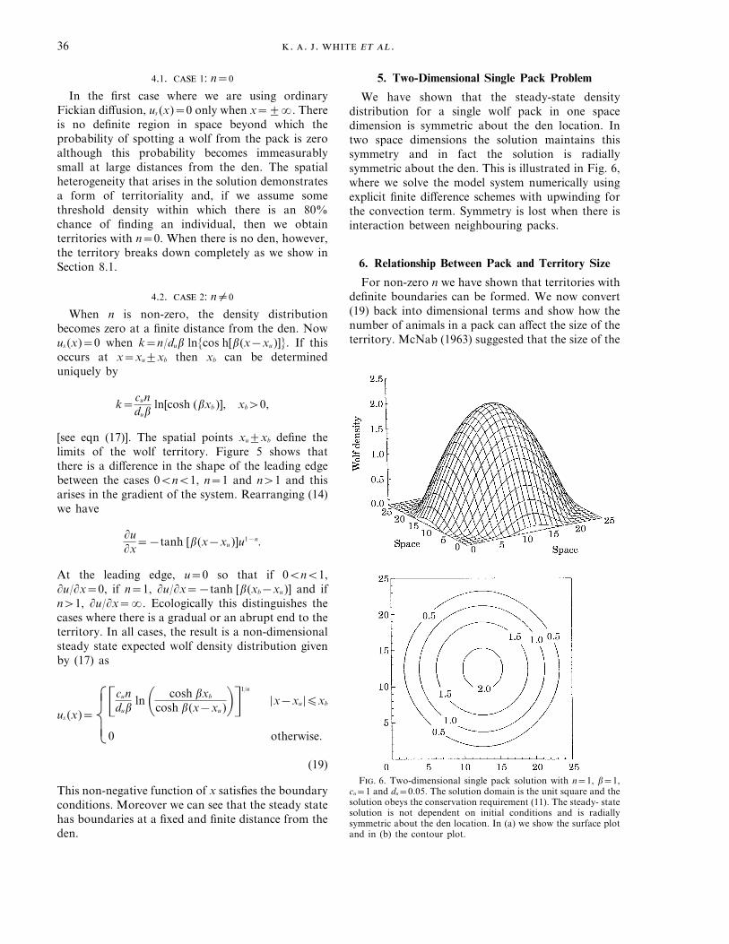
5. Two-Dimensional Single Pack Problem

We have shown that the steady-state densitydistribution for a single wolf pack in one spacedimension is symmetric about the den location. Intwo space dimensions the solution maintains thissymmetry and in fact the solution is radiallysymmetric about the den. This is illustrated in Fig. 6,where we solve the model system numerically usingexplicit finite difference schemes with upwinding forthe convection term. Symmetry is lost when there isinteraction between neighbouring packs.

6. Relationship Between Pack and Territory Size

For non-zero n we have shown that territories withdefinite boundaries can be formed. We now convert(19) back into dimensional terms and show how thenumber of animals in a pack can affect the size of theterritory. McNab (1963) suggested that the size of the

F. 6. Two-dimensional single pack solution with n=1, b=1,cu=1 and du=0.05. The solution domain is the unit square and thesolution obeys the conservation requirement (11). The steady- statesolution is not dependent on initial conditions and is radiallysymmetric about the den location. In (a) we show the surface plotand in (b) the contour plot.

37

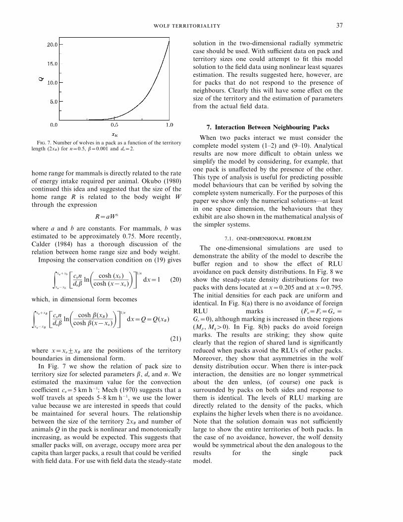
F. 7. Number of wolves in a pack as a function of the territorylength (2xB ) for n=0.5, b=0.001 and du=2.

solution in the two-dimensional radially symmetriccase should be used. With sufficient data on pack andterritory sizes one could attempt to fit this modelsolution to the field data using nonlinear least squaresestimation. The results suggested here, however, arefor packs that do not respond to the presence ofneighbours. Clearly this will have some effect on thesize of the territory and the estimation of parametersfrom the actual field data.

7. Interaction Between Neighbouring Packs

When two packs interact we must consider thecomplete model system (1–2) and (9–10). Analyticalresults are now more difficult to obtain unless wesimplify the model by considering, for example, thatone pack is unaffected by the presence of the other.This type of analysis is useful for predicting possiblemodel behaviours that can be verified by solving thecomplete system numerically. For the purposes of thispaper we show only the numerical solutions—at leastin one space dimension, the behaviours that theyexhibit are also shown in the mathematical analysis ofthe simpler systems.

7.1. -

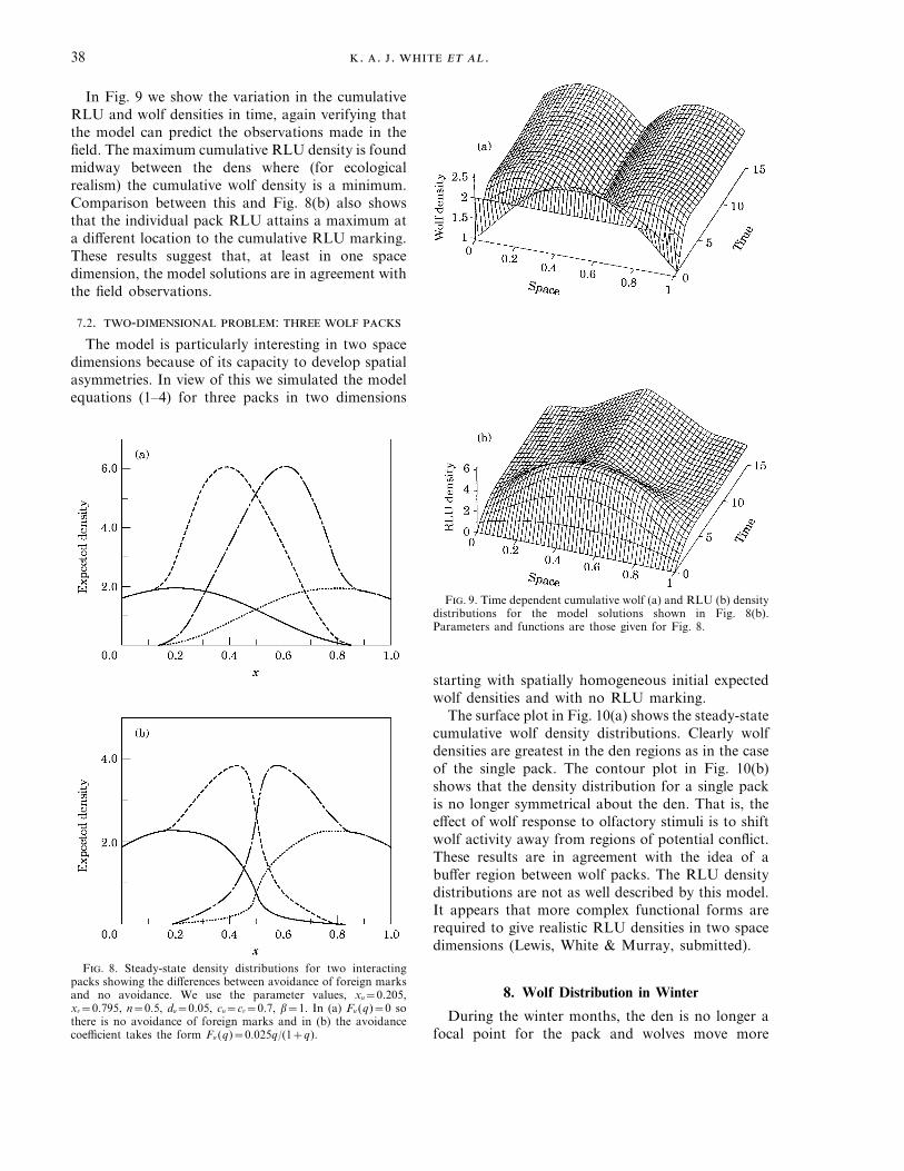
The one-dimensional simulations are used todemonstrate the ability of the model to describe thebuffer region and to show the effect of RLUavoidance on pack density distributions. In Fig. 8 weshow the steady-state density distributions for twopacks with dens located at x=0.205 and at x=0.795.The initial densities for each pack are uniform andidentical. In Fig. 8(a) there is no avoidance of foreignRLU marks (Fu=Fv=Gu =Gv=0), although marking is increased in these regions(Mp , Mqq0). In Fig. 8(b) packs do avoid foreignmarks. The results are striking; they show quiteclearly that the region of shared land is significantlyreduced when packs avoid the RLUs of other packs.Moreover, they show that asymmetries in the wolfdensity distribution occur. When there is inter-packinteraction, the densities are no longer symmetricalabout the den unless, (of course) one pack issurrounded by packs on both sides and response tothem is identical. The levels of RLU marking aredirectly related to the density of the packs, whichexplains the higher levels when there is no avoidance.Note that the solution domain was not sufficientlylarge to show the entire territories of both packs. Inthe case of no avoidance, however, the wolf densitywould be symmetrical about the den analogous to theresults for the single packmodel.

home range for mammals is directly related to the rateof energy intake required per animal. Okubo (1980)continued this idea and suggested that the size of thehome range R is related to the body weight Wthrough the expression

R=aWb

where a and b are constants. For mammals, b wasestimated to be approximately 0.75. More recently,Calder (1984) has a thorough discussion of therelation between home range size and body weight.

Imposing the conservation condition on (19) gives

gxu+xb

xu−xb$cundub

ln0 cosh (xb )cosh (x−xu )1%

1/n

dx=1 (20)

which, in dimensional form becomes

gxu+xB

xu−xB$cundub

ln0 cosh b(xB )cosh b(x−xu )1%

1/n

dx=Q=Q(xB )

(21)

where x=xu2xB are the positions of the territoryboundaries in dimensional form.

In Fig. 7 we show the relation of pack size toterritory size for selected parameters b, du and n. Weestimated the maximum value for the convectioncoefficient cu=5 km h−1; Mech (1970) suggests that awolf travels at speeds 5–8 km h−1, we use the lowervalue because we are interested in speeds that couldbe maintained for several hours. The relationshipbetween the size of the territory 2xB and number ofanimals Q in the pack is nonlinear and monotonicallyincreasing, as would be expected. This suggests thatsmaller packs will, on average, occupy more area percapita than larger packs, a result that could be verifiedwith field data. For use with field data the steady-state

. . . .38

In Fig. 9 we show the variation in the cumulativeRLU and wolf densities in time, again verifying thatthe model can predict the observations made in thefield. The maximum cumulative RLU density is foundmidway between the dens where (for ecologicalrealism) the cumulative wolf density is a minimum.Comparison between this and Fig. 8(b) also showsthat the individual pack RLU attains a maximum ata different location to the cumulative RLU marking.These results suggest that, at least in one spacedimension, the model solutions are in agreement withthe field observations.

7.2. - :

The model is particularly interesting in two spacedimensions because of its capacity to develop spatialasymmetries. In view of this we simulated the modelequations (1–4) for three packs in two dimensions

F. 9. Time dependent cumulative wolf (a) and RLU (b) densitydistributions for the model solutions shown in Fig. 8(b).Parameters and functions are those given for Fig. 8.

F. 8. Steady-state density distributions for two interactingpacks showing the differences between avoidance of foreign marksand no avoidance. We use the parameter values, xu=0.205,xv=0.795, n=0.5, du=0.05, cu=cv=0.7, b=1. In (a) Fu (q)=0 sothere is no avoidance of foreign marks and in (b) the avoidancecoefficient takes the form Fu (q)=0.025q/(1+q).

starting with spatially homogeneous initial expectedwolf densities and with no RLU marking.

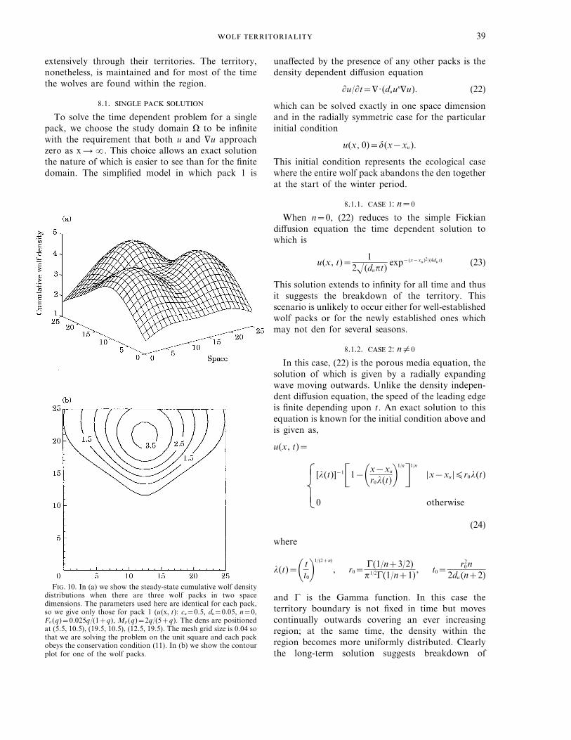
The surface plot in Fig. 10(a) shows the steady-statecumulative wolf density distributions. Clearly wolfdensities are greatest in the den regions as in the caseof the single pack. The contour plot in Fig. 10(b)shows that the density distribution for a single packis no longer symmetrical about the den. That is, theeffect of wolf response to olfactory stimuli is to shiftwolf activity away from regions of potential conflict.These results are in agreement with the idea of abuffer region between wolf packs. The RLU densitydistributions are not as well described by this model.It appears that more complex functional forms arerequired to give realistic RLU densities in two spacedimensions (Lewis, White & Murray, submitted).

8. Wolf Distribution in Winter

During the winter months, the den is no longer afocal point for the pack and wolves move more

39

extensively through their territories. The territory,nonetheless, is maintained and for most of the timethe wolves are found within the region.

8.1.

To solve the time dependent problem for a singlepack, we choose the study domain V to be infinitewith the requirement that both u and 9u approachzero as x4a. This choice allows an exact solutionthe nature of which is easier to see than for the finitedomain. The simplified model in which pack 1 is

unaffected by the presence of any other packs is thedensity dependent diffusion equation

1u/1t=9·(duun9u). (22)

which can be solved exactly in one space dimensionand in the radially symmetric case for the particularinitial condition

u(x, 0)=d(x−xu ).

This initial condition represents the ecological casewhere the entire wolf pack abandons the den togetherat the start of the winter period.

8.1.1. 1: n=0

When n=0, (22) reduces to the simple Fickiandiffusion equation the time dependent solution towhich is

u(x, t)=1

2!(dupt)exp−(x−xu )2/(4dut) (23)

This solution extends to infinity for all time and thusit suggests the breakdown of the territory. Thisscenario is unlikely to occur either for well-establishedwolf packs or for the newly established ones whichmay not den for several seasons.

8.1.2. 2: n$0

In this case, (22) is the porous media equation, thesolution of which is given by a radially expandingwave moving outwards. Unlike the density indepen-dent diffusion equation, the speed of the leading edgeis finite depending upon t. An exact solution to thisequation is known for the initial condition above andis given as,

u(x, t)=

gG

G

F

f

[l(t)]−1$1−0x−xu

r0l(t)11/n

%1/n

0

=x−xu =Er0l(t)

otherwise

(24)

where

l(t)=0 tt01

1/(2+n)

, r0=G(1/n+3/2)p1/2G(1/n+1)

, t0=r2

0n2du (n+2)

and G is the Gamma function. In this case theterritory boundary is not fixed in time but movescontinually outwards covering an ever increasingregion; at the same time, the density within theregion becomes more uniformly distributed. Clearlythe long-term solution suggests breakdown of

F. 10. In (a) we show the steady-state cumulative wolf densitydistributions when there are three wolf packs in two spacedimensions. The parameters used here are identical for each pack,so we give only those for pack 1 (u(x, t): cu=0.5, du=0.05, n=0,Fu (q)=0.025q/(1+q), Mp (q)=2q/(5+q). The dens are positionedat (5.5, 10.5), (19.5, 10.5), (12.5, 19.5). The mesh grid size is 0.04 sothat we are solving the problem on the unit square and each packobeys the conservation condition (11). In (b) we show the contourplot for one of the wolf packs.

. . . .40

territories as in the density independent case.Restricting the solution to a timescale of a few monthsonly, we can propose this as a possible description ofwolf winter movement.

8.2.

When there is no longer convection back to the denlocation, the only steady-state solution for thecomplete model system, (1–2) and (9–10) with zeroflux boundary conditions is spatially homogeneous.We now analyse the stability of this spatiallyhomogeneous solution.

To simplify the model we assume that the functionsin (1–2), are constants and that the wolf packs areidentical so that similar coefficients take on the samevalues, that is

Du (u)=Dv (v)=d Fu (q)=Fv (p)=f1

Gu (p)=Gv (q)=f2.

In addition, we suppose that the coefficients in theRLU governing equations are equal and thus set

f=1.

Moreover we choose the simplest linear functions forMp and Mq namely

Mp (q)=mq Mq (p)=mp (25)

where m is a constant. Providing that m is nottoo large, the spatially homogeneous steady-statedistribution can be written as

[us (x), vs (x), ps (x), qs (x)]=(U0, V0, P0, Q0) (26)

where

P0=U0(1+mV0)1−m2U0V0

Q0=V0(1+mU0)1−m2U0V0

(27)

with the constraint m2U0V0Q1. To simplify thesystem further, we assume that the average density ofwolves in each pack is the same so that U0=V0=W,which means that P0=Q0=W where

R=W

1−mW.

To investigate the stability of this steady-statesolution we consider the effect of imposing smallperturbations proportional to exp(st+ikx) to thehomogeneous distribution. Using standard tech-niques from linear analysis (see, for example, Murray,1989) we obtain the dispersion relation

s4+f(k2)s3+g(k2)s2+h(k2)s+s(k2)=0 (28)

where

f(k2)=2+2dk2

g(k2)=d 2k4+k2[4d−2f2W(1+mR)]+1−m2W 2

h(k2)=2d 2k4+2dk2(1−m2W2)

−2Wk2(1+mR)(f2−f1mW+f2dk2)

s(k2)=k4[d 2−d 2m2W2−2Wd(1+mR)

×(f2−f1mW)+W 2(1+mR)2(f22−f2

1 )].

Solutions s(k2) of (28) determine whether the smallperturbations will grow (R1sq0) in time and, if so,for which wavelengths.

We are interested in the possibility of spatio-temporal oscillations so we set

s(k2)=p(k2)+iq(k2).

where both p and q are real functions of k2. When wecompare the real and imaginary parts of thesubsequent expression the imaginary part gives

q=0 or q2=(h+2gp+3fp2+4p3)/(4p+f ). (29)

The case q=0 corresponds to the case where s is real,then any instabilities in space do not change withtime. The other case corresponds to the possibility oftemporal oscillations of any instability. Substitutionfor q2 into the real part of the dispersion relation givesan equation for p, namely

(4p+f )2(p4+fp3+gp2+hp+s)

+(h+2gp+3fp2+4p3)2−(4p+f )

×(h+2gp+3fp2+4p3)(g+3fp+6p2)=0. (30)

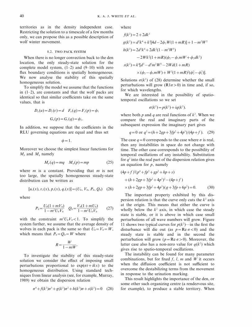
The important property exhibited by this dis-persion relation is that the curve only cuts the k2 axisat the origin. This means that either the curve iswholly below the k2 axis, in which case the steadystate is stable, or it is above in which case smallperturbations of all wave numbers will grow. Figure11 shows two typical curves for p(k2)—in the first thedisturbance will die out (as p=Re sQ0) and thesteady state is stable and in the second theperturbation will grow (p=Re sq0). Moreover, thelatter case also has a non-zero value for q(k2) whichgives rise to spatio-temporal oscillations.

The instability can be found for many parametercombinations, but for fixed f, l, m and W it occurswhen the diffusion coefficient is not sufficient toovercome the destabilizing terms from the movementin response to the urination marking.

This result highlights the importance of the den, orsome other such organizing centre (a rendezvous site,for example), to produce a stable territory. When

41

F. 11. Solution to eqn (30), the dispersion relation when W=1,m=0.5, f1=f2 and (a) d=4 and (b) d=1.

We began by analysing a simplified model whichconsiders the formation of a wolf territory when thereare no external constraints such as neighbouringpacks. In view of this, the model is perhaps of interestto the issue of wolf reintroduction presently beingconsidered in several areas of northern America suchas Yellowstone.

A report on the wolf recolonization of the GlacierNational Park (Ream et al., 1991) provides someinteresting observations both for future recolonizingpolicy and, from our point of view, for modelvalidation and adaptations. Wolf packs observed inthe study showed a preference for colonizing areaswhich had already been investigated by lone wolves.The reason for this is unclear, although olfactorystimuli left by the pioneers may provide usefulinformation as to the potential of a region. The wolfpacks in the study are thought to be closely related,but despite considerable inter-pack associations (overshort time intervals) and the availability of suitableunoccupied regions, there was clear evidence of strongpack adhesion. Our single pack model agrees with thisobservation as it suggests that packs will formterritories even in the absence of any mechanism (suchas foreign RLU marking) for territory maintenance.Pack adhesion in this case may be related to theoptimal pack size necessary both to hunt large preyand to provide sufficient social interactions for thesehighly social carnivores (Mech, 1970).

The convective flux term which describes move-ment back to the den during the summer monthsassumes that the wolves know their position relativeto the den site and will return to the den using astraight line path as observed by Mech (1970). As theconvective flux suggests that wolves know theirposition relative to the den, it can also be interpretedas one component of a wolf’s cognitive map. Peters(1979) interpreted field observations by suggestingthat wolves develop a mental map of their territorywhich is continually being reinforced. Within theterritory, RLU markings are found most often alongwolf trails (Peters & Mech, 1975), indicating thatolfactory stimuli may play an essential role inmaintaining and updating this cognitive map.

The importance of the cognitive map is highlightedby the analysis in Section 8.2 which showed that, inthe absence of a den, the only steady state solutionwas spatially homogeneous. That is, that steady-statespatial heterogeneity, which represents the mainten-ance of pack territories, only occurs when theconvective flux is non-zero. Thus long-term winterbehaviour indicates territory breakdown. On ashorter time scale of several months, however, themodel can be reasonably used to describe winter

there is no den, even in the simplest case describedhere, a small perturbation to the steady-state wolfdistribution can lead to spatio–temporal oscillationsand thus no formation of territories. In fact, incontrast to the case where there is a den, thedistribution is dependent upon the initial wolf andRLU distribution.

9. Discussion

In this paper we have presented a new math-ematical model system to describe the territorialnature of movement. The research was motivated inpart by the extensive field studies carried out onwolves in N.E. Minnesota (see, for example, Mech,1970; van Ballenberghe et al., 1975). Several aspectsof the field ecology have been captured by the modelsolution.

. . . .42

distributions, as shown in the results of Section 8.1.1where the winter wolf distribution consists of aradially expanding wave moving outwards with somefinite speed. This suggests that the pack is movingmore extensively through the territory (expecteddensity becomes more homogeneous) and that thereis a greater chance of a wolf trespassing into the bufferzone or some neighbouring territory. Field obser-vations indicate that when the rendezvous sites areabandoned, the pack moves extensively throughoutthe territory (van Ballenberghe et al., 1975) whichagrees with the more uniform use of land predicted bythe model. Clearly one drawback of this model is thatthere is no form of cognitive map associated with thewinter wolf behaviour. We are investigating ways toamend the present model systems to maintain someform of cognitive map during the winter months. Onepossible scenario is that the wolves move back tomore familiar regions during the winter so that a con-vective flux can be based on the centre of mass ofthe expected wolf density (Lewis, White & Murray,submitted).

When considering the interaction of several packs,scent marking is thought to have an important role inmaintaining territories. The role of scent marking inthe model solutions was to break the symmetry ofwolf density distributions about the den locations. Inthis way it allowed for the possibility of buffer regionswhere wolves are scarce but where RLU marking isat its highest density. In one space dimension, themodel solutions showed good agreement with the fieldecology. In two dimensions, however, although bufferregions were formed with low wolf densities, thecumulative RLU density did not increase significantlyin this region. We are now investigating other formsfor the functions related to wolf response to scentmarking. In particular we are considering the idea ofa threshold phenomena where response to foreign (orfriendly) marks is only significant when the densityexceeds some critical level. Preliminary results (with aslightly different model formulation) indicate that ifwe use functional forms of this nature, the cumulativeRLU density may attain its maximum value in thebuffer region (Lewis, White & Murray, submitted).The importance of the functional response of wolvesto scent marking is very interesting—moreover, it isone which could be investigated further by controlledfield experiments.

Movement back to an organizing centre (whichcan be interpreted as a response to a cognitivemap) was clearly very important for obtaining aspatially heterogeneous steady-state solution (terri-tory). There are, however, several other possiblemechanisms for maintaining territory structure

without a focal point. For example, newly formedwolf pairs may form a territory for 2 years beforeproducing young (and thus constructing a den site);similarly for sterile pairs and established pairs orpacks who maintain their territories even in yearswhere there is no reproduction (David L. Mech, pers.comm.).

If surrounding territories already exist, then thenon-reproductive pair will be subject to some form offoreign RLU spatial patterning. In this case, theterritories may be formed or maintained merely by aresponse to local densities of scent marks. A morelong range form of territorial behaviour is that ofhowling. Harrington & Mech (1983) present results ofa field study which show that wolf response tohowling, both in terms of reply and movement, isindependent of wolf position within the territory anddepends rather on the immediate social and ecologicalcircumstances, such as the presence of a prey kill orthat of young pups. This mechanism for territorymaintenance differs from scent marking both in itsspatial and temporal properties but, along with wolfpreference for familiar regions, seems capable ofmaintaining exclusive territories without the need foran organizing centre. Clearly it would be interestingto compare the territory structures formed in the caseof a short range, long lasting mechanism (RLUmarking) and for a long range, short time mechanism(howling).

In another study, Ciucci & Mech (1992) showedthat dens situated within the central portion ofterritories were randomly located relative to theterritory centres although, in larger territories, thedens did tend to be more centrally located. In thenumerical simulations shown in Section 7, the denpositions were chosen arbitrarily. The resulting wolfdistributions were such that the den was positionedsomewhere in the central region of the wolf territory,suggesting some agreement with the field work.Further investigation is necessary to determine theextent of model agreement.

The discussion would not be complete withoutsome comparison of the model presented andanalysed here with that of Lewis & Murray (1993). Asmentioned in the introduction, the forms of the twomodels are similar, both being nonlinear partialdifferential equations with diffusive and convectivefluxes. The qualitative behaviours differ, however, inthe way in which territories form because the modelof Lewis & Murray (1993) requires the presence offoreign wolf packs (or at least foreign RLU markings)in order to obtain a territory. In the absence of sucholfactory stimuli, their model reduces to the diffusionequation which suggests that the territory mechanism

43

breaks down and wolves from all packs moverandomly around. In the model proposed here, theformation of a territory depends only upon the packitself (supported by van Ballenberghe et al., 1975) andforeign markings serve to determine the size, shapeand maintenance of the territory.

This work (K.A.J.W., J.D.M.) was supported in part byU.S. National Science Foundation Grant DMS 9296848and (M.A.L.) by U.S. National Science Foundation GrantDMS 9222533.

REFERENCES

B, P. J., B, F. & B, P. (1991). A model forterritory and group formation in a heterogeneous habitat. J.theor. Biol. 148, 445–468.

B, S. (1989). An olfactory orientation model formammals’ movements in their home ranges. J. theor. Biol. 139,

379–388.B, J. L. & O, G. H. (1970). Spacing patterns in mobile

animals. Ann. Rev. Ecol. Syst. 1, 239–262.C, W. A. III. (1984). Size, Function and Life History.

Cambridge, MA: Harvard University Press.C, E. L. (1976). Optimal foraging, the marginal value

theorem. Theor. Pop. Biol. 9, 129–136.C, A. P. (1976). Analysing shapes of foraging areas: some

ecological and economic theories. Ann. Rev. Ecol. Syst. 7,

235–257.C, P. & M, L. D. (1992). Selection of wolf dens in relation

to winter territories in northeastern Minnesota. J. Mammal. 73,

899–905.D, B. A. C. & R, K. (1983). A home range model

incorporating biological attraction points. J. Anim. Ecol. 52,

69–81.E-E, I. (1970). Ethology: the biology of behaviour. New

York: Holt, Rinehart and Winston.E, J. T. (1957). Defended area? A critique of the territory

concept and of conventional thinking. Ibis 99, 352.G, D. & O, A. (in press). Modelling social animal

aggregations. In: Animal Aggregation: Analysis, Theory, andModelling (tentative title). Cambridge: Cambridge UniversityPress.

H, F. H. & M, L. D. (1983). Wolf pack spacing:Howling as a territory-independent spacing mechanism in aterritorial population. Behav. Ecol. Sociobiol. 12, 161–168.

H, R. L. & M, L. D. (1976). White-tailed deer

migration and its role in wolf predation. J. Wildl. Manage. 40,

429–441.L, M. A. & M, J. D. (1993). Modelling territoriality and

wolf-deer interactions. Nature 366, 738–740.M, D. W. (1983). The ecology of carnivore social

behaviour. Nature 301, 379–384.M, L. D. (1970). The Ecology and Behavior of an Endangered

Species. Garden City, N.Y.: Natural History Press.M, L.D. (1977a). Productivity, mortality and population trends

of wolves in northeastern Minnesota. J. Mammal. 58(4), 559–574.M, L. D. (1977b). Wolf-pack buffer zones as prey reservoirs.

Science 198, 320–321.M, L. D. (1977c). Population trend and winter deer

consumption in a Minnesota wolf pack. In: Proceedings of the1975 Predator Symposium (Philips, R. L. & Jonkel, L., eds)University of Montana, Missoula, Montana.

MN, B. K. (1963). Bio-energetics and the determination ofhome range size. Am. Nat. 97, 133–140.

M, J. D. (1993). Mathematical Biology, 3rd Edn. Heidelberg:Springer-Verlag.

N, G. K. (1939). The role of dominance on the social life ofbirds. Auk 56, 263–273.

O, A. (1980). Diffusion and Ecological Problems: Mathemati-cal Models. Berlin: Springer-Verlag.

O, A. (1986). Dynamical aspects of animal grouping: swarms,schools, flocks and herds. Adv. Biophys. 22, 1–94.

P, R. (1979). Mental maps in wolf territoriality. In: TheBehavior and Ecology of Wolves (Klinghammer, E., ed.),pp. 119–152. New York: Garland Press.

P, F. A. (1959). Numbers, breeding schedule, andterritoriality in pectoral sandpipers of northern Alaska. Condor61, 233–264.

P, H. P. & H, A. I. (1990). Optimal patch use bya territorial forager, J. theor. Biol. 145, 343–353.

R, R. R., F, M. W., B, D. K. & P, D. H.(1991). Population dynamics and home range changes in acolonizing wolf population. In: The Greater YellowstoneEcosystem: Redefining America’s Wilderness Heritage (Keiter,R. B., Boyce, M. S., eds), pp. 349–366. Binghamton NY:Vail-Ballon Press.

S, N., K, K. & T, E. (1979). Spatialsegregation of interacting species. J. theor. Biol. 79, 83–99.

S, J. G. (1951). Random dispersal in theoretical popu-lations. Biometrika 38, 196–218.

T, R. J. & P, P. J. (1991). Territory boundary avoidanceas a stabilising factor in wolf–deer interactions. Theor. Pop. Biol.39, 115–128.

B, V., E, A. W. & B, D. (1975).Ecology of the timber wolf in Northeastern Minnesota. WildlifeMonographs 43, 1–43.

W, W. (1975). Comparison of several probabilistic homerange models. J. Wildl. Manage. 39, 118–123.