HAL Id: insu-00843306https://hal-insu.archives-ouvertes.fr/insu-00843306

Submitted on 11 Jan 2014

HAL is a multi-disciplinary open accessarchive for the deposit and dissemination of sci-entific research documents, whether they are pub-lished or not. The documents may come fromteaching and research institutions in France orabroad, or from public or private research centers.

L’archive ouverte pluridisciplinaire HAL, estdestinée au dépôt et à la diffusion de documentsscientifiques de niveau recherche, publiés ou non,émanant des établissements d’enseignement et derecherche français ou étrangers, des laboratoirespublics ou privés.

A model of fracture nucleation, growth and arrest, andconsequences for fracture density and scaling

Philippe Davy, Romain Le Goc, Caroline Darcel

To cite this version:Philippe Davy, Romain Le Goc, Caroline Darcel. A model of fracture nucleation, growth and ar-rest, and consequences for fracture density and scaling. Journal of Geophysical Research, AmericanGeophysical Union, 2013, 118 (4), pp.1393-1407. <10.1002/jgrb.50120>. <insu-00843306>

A model of fracture nucleation, growth and arrest, andconsequences for fracture density and scaling

Philippe Davy,1 Romain Le Goc,2 and Caroline Darcel2

Received 9 May 2012; revised 3 January 2013; accepted 1 February 2013; published 25 April 2013.

[1] In order to improve discrete fracture network (DFN) models, which areincreasingly required into groundwater and rock mechanics applications, we propose anew DFN modeling based on the evolution of fracture network formation—nucleation,growth, and arrest—with simplified mechanical rules. The central idea of the modelrelies on the mechanical role played by large fractures in stopping the growth ofsmaller ones. The modeling framework combines, in a time-wise approach, fracturenucleation, growth, and arrest. It yields two main regimes. Below a certain criticalscale, the density distribution of fracture sizes is a power law with a scaling exponentdirectly derived from the growth law and nuclei properties; above the critical scale, aquasi-universal self-similar regime establishes with a self-similar scaling. The densityterm of the dense regime is related to the details of arrest rule and to the orientationdistribution of the fractures. The DFN model, so defined, is fully consistent with fieldcases former studied. Unlike more usual stochastic DFN models, ours is based on asimplified description of fracture interactions, which eventually reproduces themultiscale self-similar fracture size distribution often observed and reported in theliterature. The model is a potential significant step forward for further applications togroundwater flow and rock mechanical issues.

Citation: Davy, P., R. Le Goc, and C. Darcel (2013), A model of fracture nucleation, growth and arrest, andconsequences for fracture density and scaling, J. Geophys. Res. Solid Earth, 118, 1393–1407, doi:10.1002/jgrb.50120.

1. Introduction

[2] Fractures are ubiquitous in geological systems and keystructures for groundwater flow and mechanical resistance ofrocks. It is now clearly demonstrated that the density offractures and their spatial organization are controllingflow and mechanical properties of rock masses. Thus, mostof the predictions in hydrogeology, seismology, andgeomechanics—with application to water resources, mining,geothermal industry, deep waste isolation, among others—are dependent on the pertinence of the fracture networkdescription, although the degree to which it must be is stillan issue [Berkowitz et al., 2000b; Caumon et al., 2009; deDreuzy et al., 2001a, b; Paluszny and Matthai, 2010;Svensson, 2001].[3] An intrinsic difficulty is to deal with a range of fracture

scales that cover several orders of magnitudes in anytectonic system, from microfractures smaller than micro- tomillimeters to tectonic faults larger than hundreds of metersto kilometers. The apparent similarity between fracture

patterns at different scales has long been recognized bygeologists [Tchalenko, 1970] and has led to apply fractalscaling concepts to fracture networks: fracture patterns arelikely characterized by fractal dimensions; fracture lengthdistributions appear to be adequately fitted by power laws(the only mathematical functions that do not require a scaleparameter) from meter to tens of kilometer scales [see thecompilation by Bonnet et al., 2001]. Whatever the modelof fracture organization is, taking account of this large rangeof facture scales in mechanical or flow models requireseither high-resolution underground imagery of fracturenetworks or the development of pertinent stochastic fracturenetwork models to replace the lack of observation. Since theformer is still out of reach, most models of fluid flow andtransport processes are based on Statistical Discrete FractureNetwork methods (DFN) [see Jing et al., 2007 for a review],which are statistical generation methods conditioned tolength and orientation frequency distribution. The positionsof fractures are generally assumed to be random, but thisassumption needs to be further proven since it does notreflect the complexity of geological patterns [Ackermannand Schlische, 1997; Darcel et al., 2003a].[4] The aim of this paper is to develop a stochastic DFN

modeling framework able to match both important propertiesthat constitute a large part of the complexity of geologicalfracture networks: the fracture-to-fracture spatial interactionsand the scaling relationships between fracture lengths anddensities over several orders of magnitude. Both are criticalfor defining the DFN connectivity [Berkowitz et al., 2000a;

1Geosciences Rennes, CNRS, University of Rennes 1, Campus deBeaulieu, Rennes, France.

2ITASCA Consultants, SAS, 64 chemin des Mouilles, Ecully, France.

Corresponding author: P. Davy, Geosciences Rennes, CNRS, Universityof Rennes 1, Campus de Beaulieu, Rennes, France. (philippe.davy@univ-rennes1.fr)

©2013. American Geophysical Union. All Rights Reserved.2169-9313/13/10.1002/jgrb.50120

1393

JOURNAL OF GEOPHYSICAL RESEARCH: SOLID EARTH, VOL. 118, 1393–1407, doi:10.1002/jgrb.50120, 2013

Bour and Davy, 1997, 1998; Darcel et al., 2003b; Davy et al.,2006a; de Dreuzy et al., 2001a]. The method we develop isbased on a simplified modeling of the fracturing processes,which still enables handling millions of fractures in 3D.It relies on the main stages of fracture evolution: nucleation,growth, and arrest. This time-wise process differs fromclassical DFN models that only “bootstrap” the currentgeological stage.[5] The basic mechanical concepts are derived from the

“likely” universal model of fracture scaling (UFM) of [Davyet al., 2010], which theoretically derives a fracture-sizedensity distribution model from simplified rules of fracturearrest. The model, which depends only on the topologicalnetwork dimension D and on a dimensionless parameter g,was found to be a good fit for a large number of fracturedatasets, whether they are made of faults or joints. The basicidea is to highlight the mechanical role of large fractures instopping the growth of smaller ones. A strict causalityrule—a small fracture cannot cross a larger one, but thereverse is likely to occur—obviously simplifies the mechan-ical reasons for stopping fracture growth [Crampin, 1994,1999; Pollard and Aydin, 1988; Renshaw and Pollard,1994; Renshaw and Park, 1997; Renshaw et al., 2003], butit renders the main mechanical interactions [Nur, 1982;Segall and Pollard, 1983; Spyropoulos et al., 1999] and isstatistically consistent with the large number of commonlyobserved T-like fracture intersections. Additionally andpragmatically, it is easily manageable in simple stochasticmodels. Davy et al. [2010] demonstrated that this pseudo-mechanical rule entails a quasi-universal density distributionof fracture sizes, which takes the form of a power law with afixed exponent and a quasi-fixed density term. The reasonwhy this universal distribution emerges is that thefracture length once arrested is about the distance to itslarger neighbor. This geometrical rule fixes the density oflarge fractures. If fractures are smaller than the distance tothe nearest neighbor, they are not suppose to interactmechanically, and their length distribution is then controlledby the growth law of isolated fractures (dilute regime).[6] Davy et al. [2010] show that this two-regime length

distribution is consistent with the statistics derived from afew detailed mapping studies of natural outcrops orexperiments, with a transition between the “dense” large-length UFM distribution and the “dilute” small-length onethat was observed to vary from 1–10 m for joint networksto ~20 km for the San Andreas fault system. They also showthat this so-called UFM generation model leads tonetworks, the connectivity and flow properties of whichare significantly different from the classical random(Poisson statistics) model, even if the fracture lengthdistributions are identical. This emphasizes the need todevelop this kind of DFN models that mimic fracturingprocesses.[7] In this paper, we discuss possible nucleation, growth,

and arrest rules that “naturally” generate the scaling lawsobserved in fracture networks. As in Davy et al. [2010],we use the fracture-length density distribution n(l, L) as thestatistical descriptor of fracture patterns. n(l, L) dl is thenumber of fractures of length in the range [l, l+ dl] withina volume of typical size L. For geological fracture networks,n(l, L) has been found to be adequately fitted by thefollowing scaling laws valid over a large range of scales:

n l;Lð Þ ¼ a l�aLD; (1)

where D is formally the mass (or correlation) dimension ofthe fracture-center network that is smaller or equal to thetopological dimension [see Bonnet et al., 2001; Bour et al.,2002 for more explanations]; a is the power-law lengthscaling exponent, and a a the density term that is likelyincreasing during fracture growth.[8] Note that this paper is the first step towards a complete

DFN methodology that can be applied to the modeling offlow and mechanical properties of fracture-controlledgeologic sites. Such applications require additional informa-tion on fracture aperture (for hydraulic properties), strength,and elastic parameters (mechanical properties) that we donot discuss in this paper. It is no insignificant matter,considering the critical role of fracture transmissivitydistribution on the macroscopic flow and transportproperties [de Dreuzy et al., 2001a, 2001b, 2002; de Dreuzyet al., 2010].

2. The Complete Model of Fracture Formation:Nucleation, Growth, and Arrest

[9] Fracturing is a feedback-loop process where thegrowth of fractures modifies their growth properties(through elastic stresses within the unfractured material)[Atkinson, 1987; Bourne and Willemse, 2001; Ingraffea,1987; Kachanov and Laures, 1989; Pollard and Aydin,1988; Segall, 1984a,1984b]. The complexity of this dynamicprocess is directly related to the complexity of the develop-ing network structure. This (somewhat trivial) statementillustrates the difficulty to simplify a process that leads innature to networks with fracture sizes spanning over ordersof magnitudes [Bonnet et al., 2001].[10] In addition to describing the geometry and scaling

properties of fractured systems, a DFN description is alsorelevant to analyze the main mechanical interactions offracture networks that are basic to define fracture growth[Kachanov and Laures, 1989; Kachanov, 2003]. Althoughless versatile than a continuum-mechanics approach(some assumptions about the shape of fractures and thehomogeneity of elastic properties are required to solve themechanical problem), the DFN is particularly well suitedto describe the three main stages of the complete fractureformation stages—(i) nucleation of fractures, (ii) growth,that is, propagation of fractures, and (iii) fracture arrest—and to analyze the properties of the resulting network.[11] A few studies have put emphasis on the relationship

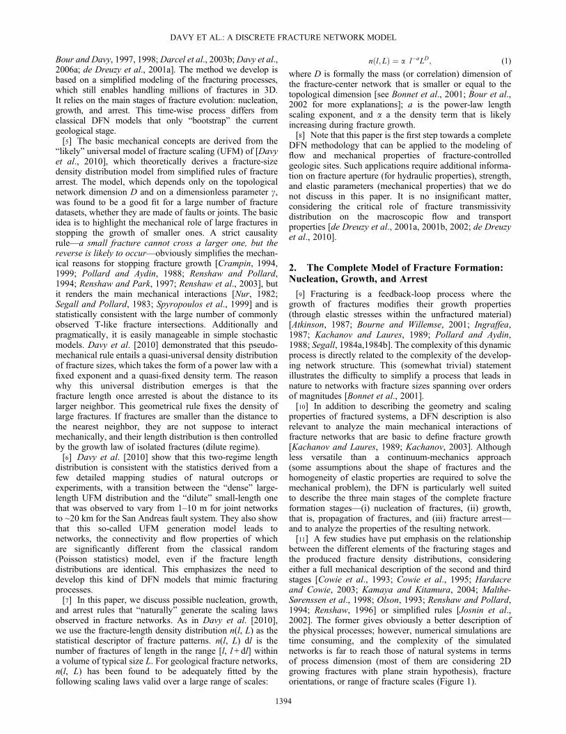
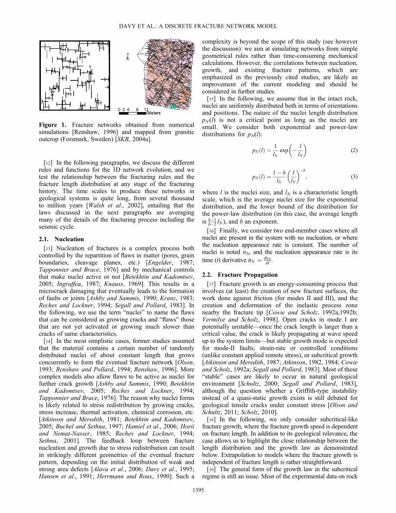
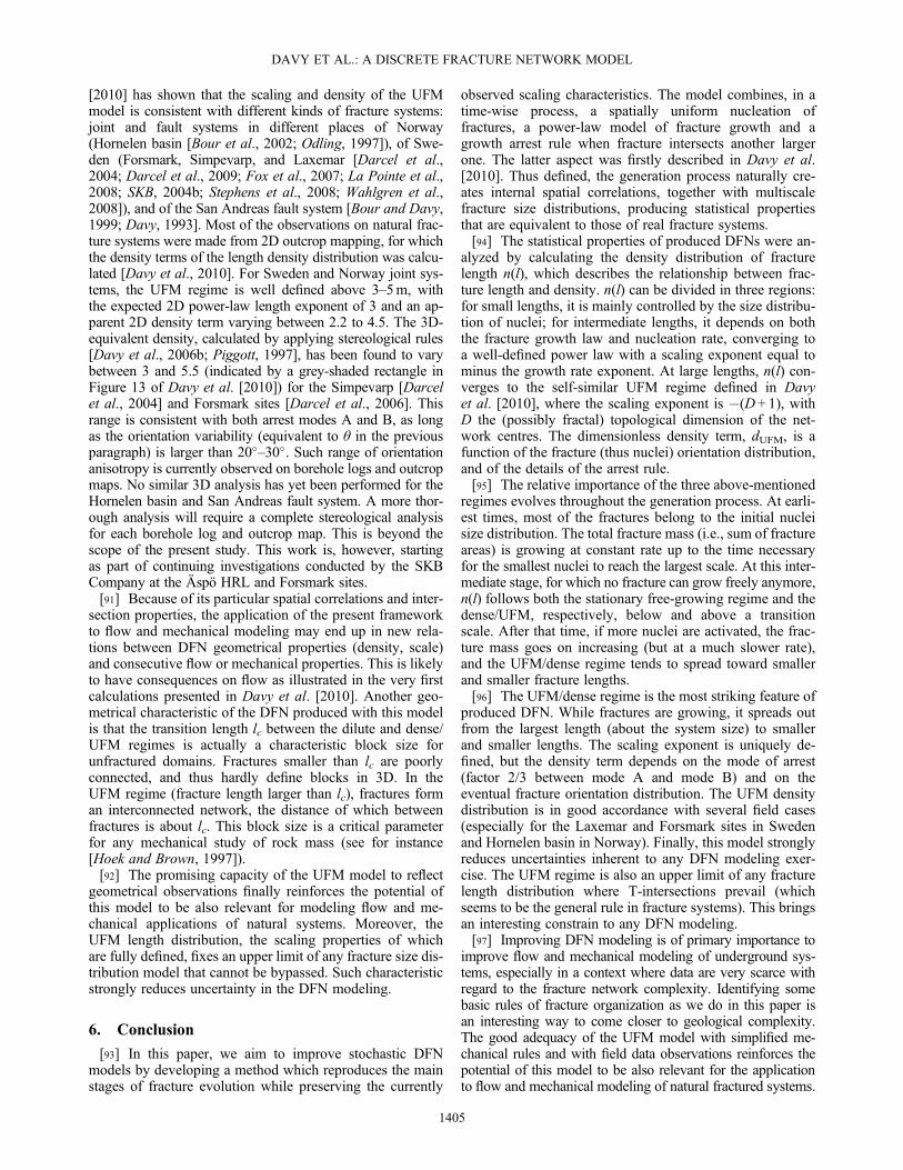
between the different elements of the fracturing stages andthe produced fracture density distributions, consideringeither a full mechanical description of the second and thirdstages [Cowie et al., 1993; Cowie et al., 1995; Hardacreand Cowie, 2003; Kamaya and Kitamura, 2004; Malthe-Sørenssen et al., 1998; Olson, 1993; Renshaw and Pollard,1994; Renshaw, 1996] or simplified rules [Josnin et al.,2002]. The former gives obviously a better description ofthe physical processes; however, numerical simulations aretime consuming, and the complexity of the simulatednetworks is far to reach those of natural systems in termsof process dimension (most of them are considering 2Dgrowing fractures with plane strain hypothesis), fractureorientations, or range of fracture scales (Figure 1).

DAVY ET AL.: A DISCRETE FRACTURE NETWORK MODEL

1394

[12] In the following paragraphs, we discuss the differentrules and functions for the 3D network evolution, and wetest the relationship between the fracturing rules and thefracture length distribution at any stage of the fracturinghistory. The time scales to produce these networks ingeological systems is quite long, from several thousandto million years [Walsh et al., 2002], entailing that thelaws discussed in the next paragraphs are averagingmany of the details of the fracturing process including theseismic cycle.

2.1. Nucleation

[13] Nucleation of fractures is a complex process bothcontrolled by the repartition of flaws in matter (pores, grainboundaries, cleavage planes, etc.) [Engelder, 1987;Tapponnier and Brace, 1976] and by mechanical controlsthat make nuclei active or not [Betekhtin and Kadomtsev,2005; Ingraffea, 1987; Knauss, 1969]. This results in amicrocrack damaging that eventually leads to the formationof faults or joints [Ashby and Sammis, 1990; Kranz, 1983;Reches and Lockner, 1994; Segall and Pollard, 1983]. Inthe following, we use the term “nuclei” to name the flawsthat can be considered as growing cracks and “flaws” thosethat are not yet activated or growing much slower thancracks of same characteristics.[14] In the most simplistic cases, former studies assumed

that the material contains a certain number of randomlydistributed nuclei of about constant length that growsconcurrently to form the eventual fracture network [Olson,1993; Renshaw and Pollard, 1994; Renshaw, 1996]. Morecomplex models also allow flaws to be active as nuclei forfurther crack growth [Ashby and Sammis, 1990; Betekhtinand Kadomtsev, 2005; Reches and Lockner, 1994;Tapponnier and Brace, 1976]. The reason why nuclei formsis likely related to stress redistribution by growing cracks,stress increase, thermal activation, chemical corrosion, etc.[Atkinson and Meredith, 1981; Betekhtin and Kadomtsev,2005; Buchel and Sethna, 1997; Hamiel et al., 2006; Horiiand Nemat-Nasser, 1985; Reches and Lockner, 1994;Sethna, 2001]. The feedback loop between fracturenucleation and growth due to stress redistribution can resultin strikingly different geometries of the eventual fracturepattern, depending on the initial distribution of weak andstrong area defects [Alava et al., 2006; Davy et al., 1995;Hansen et al., 1991; Herrmann and Roux, 1990]. Such a

complexity is beyond the scope of this study (see howeverthe discussion): we aim at simulating networks from simplegeometrical rules rather than time-consuming mechanicalcalculations. However, the correlations between nucleation,growth, and existing fracture patterns, which areemphasized in the previously cited studies, are likely animprovement of the current modeling and should beconsidered in further studies.[15] In the following, we assume that in the intact rock,

nuclei are uniformly distributed both in terms of orientationsand positions. The nature of the nuclei length distributionpN (l) is not a critical point as long as the nuclei aresmall. We consider both exponential and power-lawdistributions for pN(l):

pN lð Þ ¼ 1

lNexp � l

lN

� �(2)

pN lð Þ ¼ 1� b

lN

l

lN

� ��b

; (3)

where l is the nuclei size, and lN is a characteristic lengthscale, which is the average nuclei size for the exponentialdistribution, and the lower bound of the distribution forthe power-law distribution (in this case, the average lengthis b�1

b�2 lN ), and b an exponent.

[16] Finally, we consider two end-member cases where allnuclei are present in the system with no nucleation, or wherethe nucleation appearance rate is constant. The number ofnuclei is noted nN, and the nucleation appearance rate is itstime (t) derivative _nN ¼ dnN

dt .

2.2. Fracture Propagation

[17] Fracture growth is an energy-consuming process thatinvolves (at least) the creation of new fracture surfaces, thework done against friction (for modes II and III), and thecreation and deformation of the inelastic process zonenearby the fracture tip [Cowie and Scholz, 1992a,1992b;Vermilye and Scholz, 1998]. Open cracks in mode I arepotentially unstable—once the crack length is larger than acritical value, the crack is likely propagating at wave speedup to the system limits—but stable growth mode is expectedfor mode-II faults, strain-rate or controlled conditions(unlike constant applied remote stress), or subcritical growth[Atkinson and Meredith, 1987; Atkinson, 1982, 1984; Cowieand Scholz, 1992a; Segall and Pollard, 1983]. Most of these“stable” cases are likely to occur in natural geologicalenvironment [Schultz, 2000; Segall and Pollard, 1983],although the question whether a Griffith-type instabilityinstead of a quasi-static growth exists is still debated forgeological tensile cracks under constant stress [Olson andSchultz, 2011; Scholz, 2010].[18] In the following, we only consider subcritical-like

fracture growth, where the fracture growth speed is dependenton fracture length. In addition to its geological relevance, thecase allows us to highlight the close relationship between thelength distribution and the growth law as demonstratedbelow. Extrapolation to models where the fracture growth isindependent of fracture length is rather straightforward.[19] The general form of the growth law in the subcritical

regime is still an issue. Most of the experimental data on rock

Figure 1. Fracture networks obtained from numericalsimulations [Renshaw, 1996] and mapped from graniticoutcrop (Forsmark, Sweden) [SKB, 2004a].

DAVY ET AL.: A DISCRETE FRACTURE NETWORK MODEL

1395

samples have been obtained for mode I [Atkinson, 1984], andonly a few for modes II and III [Ko and Kemeny, 2011] withresults consistent with mode I. The main fitting or theoreticalmodels are either power law or exponential model.[20] The power law was introduced by Charles [1958]

(and known as the Charles’ law) and widely used in theliterature to describe the crack tip velocity in the subcriticalregime: v ¼ dl

dt ¼ CKm [Atkinson, 1984; Das and Scholz,1981; Kamaya and Kitamura, 2004; Newman and Raju,1981], where K is the stress intensity factor, and m is thestress-corrosion index or the subcritical fracture growth index.m can vary widely and depends on the fracture growthmechanism and rock type [Atkinson, 1987]. Olson [2003,2004], shows that the density and organization of fracturesare directly related to m; when m goes to infinity, only thelargest nuclei propagates, while all fractures develop indepen-dently of their length when m is 0. If fractures are relativelyindependent of each others, the value K is proportional tothe square root of the fracture length, so that the fracture-growth-rate equation now writes:

v lð Þ ¼ dl

dt¼ Cla; (4)

where a is the growth exponent, and C is a parameterassumed constant, which depends on the remote stress.[21] Exponential models were based on thermodynamic

theories developed for slow fracture growth in mode I[Darot and Gueguen, 1986; Dove, 1995; Vanel et al.,2009]. The crack tip velocity is expected to be proportionalto an exponential Arrhenius-type term, where the activationenergy, G, is the energy release rate during growth.Considering the dependency of G on the fracture length l,these models predict that the fracture growth rate shouldincrease exponentially with length:

v ¼ dl

dt¼ C exp

l

lc

� �; (5)

where both constant C and lc depend on temperature,stress, and elastic properties of rock materials [Vanel et al.,2009]. Note that there is another exponential expression,where the fracture growth rate is proportional to theexponential function of the intensity factor K, which in turnis proportional to the square root of the fracture lengthl [Dove, 1995].[22] Whatever the growth law, because of its fast increase

with length fractures become infinite in a finite time. The so-called time to rupture tr is characteristic of the growth law

and depends on the initial nuclei length lN: tr ¼ lN 1�a

a�1ð ÞC for

the power law (equation ((4)), and tr ¼ lcC exp � lN

lc

� �for

the exponential law (equation ((5)).[23] In the next paragraph, wewill discuss the fracture length

distribution produced by the growth equations ((4) and ((5).

2.3. Fracture Size Distribution for Freely GrowingFractures

[24] The fracture size distribution can be calculated from abalance between time t and t+ dt. A fracture set n(l,t)� dl atthe time t will grow to n(l+ v(l)dt, t+ dt)� dl ’ at the timet + dt, where dl0 is the transformation of the length rangedl by the fracture growth: dl’ ¼ dl � 1þ dv

dl dt� �

; the fracture

balance must also incorporate the set of nuclei producedduring dt: _nN tð ÞpN l þ v lð Þdtð Þ � dl’ � dt . In the limit whereboth dl and dt go to 0, this gives the general differentialequation [see also Sano et al., 1981; Sornette and Davy, 1991]:

@n

@tþ @ vnð Þ

@l¼ _nN tð ÞpN lð Þ: (6)

a) Case where the nucleation rate _nN is constant and non-nil

[25] This equation has a stationary solution if both _nN andv(l ) are time independent and non-nil:

nst lð Þ ¼ _nNv lð Þ 1� PN lð Þð Þ: (7)

with PN lð Þ ¼Z 1

lpN lð Þdl is the complementary cumulative

probability distribution of nuclei, which is supposed to vanishrapidly. Thus, for all lengths such as PN(l)<<1, the stationarydistribution length nst lð Þ is the ratio nst lð Þ ¼ _nN

v lð Þ, proportionalto the nucleation rate by the inverse of the growth rate func-tion. An exponentially increasing growth rate (see previousparagraph) will eventually produce an exponentially decreas-ing distribution length, while Charles’ law is consistent with apower law:

nst l≫lNð Þ ¼ _nNC

l�a; (8)

which is only controlled by the parameters C and a of thegrowth law and by the nucleation rate _nN , independently ofthe nuclei length distribution.[26] There is no obvious analytical solution for the

nonstationary regime, but the solution may be approachedby posing: n l; tð Þ ¼ _nN

v lð Þ ey l; tð Þ þ 1� PN lð Þð Þ , with ey l; tð Þ a

non-stationary dimensionless term that obeys a quite simpletransport equation:

1

v lð Þ@ey@t

þ @ey@l

¼ 0: (9)

v(l), the speed term of the above equation, is increasingwith l; we thus expect the stationary regime to be reachedfaster for large lengths than for small ones.[27] We can also conjecture about the time scale of the

process. Indeed, the above equation shows that v(l) is theonly function that links time and length scales. In thisdynamical system, the natural length scale is the nucleilength lN. A natural time scale would be the ratio to ¼ lN

v lNð Þ,which characterizes the very first stage of nuclei growth.This time scale is of the same order of magnitude as the timeto rupture tr as defined in the previous paragraph (tr ¼ to

a�1 forthe power-law equation, and tr ¼ to

lNlc

for the exponentialfunction); it is likely the time to reach the stationary solution.

b) Case where N nuclei are present at t = 0 and nonucleation rate

DAVY ET AL.: A DISCRETE FRACTURE NETWORK MODEL

1396

[28] If all fractures are present since beginning, the lengthdistribution at any time t reflects the shift of the initial nucleilength distribution pN(l) by the growth rate equations ((4)and ((5). The density distribution of fracture at any timet is directly related to the initial nuclei length distributionat t = 0 by a one-to-one correspondence relationship:

n lð Þ dl ¼ n lt¼0ð Þdlt¼0;

where lt= 0 is the corresponding nuclei length. The initialdensity distribution n(lt= 0) is the product of the total numberof nuclei N by the frequency distribution of nuclei size pN.The fracture length l(t) is obtained by integrating thegrowth-rate equation from its initial value: For the power-law growth model (equation ((4)), this gives:

l tð Þ ¼ lt¼01�a � a� 1ð ÞCt� � 1

1�a:

[29] Thus, we can derive n(l) at any time t by derivingl with respect to lt = 0. We obtain the following expressionfor n(l):

n lð Þ ¼ N � pN lt¼0ð Þ � l

lt¼0

� ��a

and lt¼0 ¼ l1�a þ a� 1ð ÞCtð Þ1

1� a:

(10)

[30] As long as l1� a<< (a� 1)Ct (i.e., t is large enough),n(l) is a power law, the exponent of which is minus thegrowth-rate exponent a:

n lð Þ ¼ N �pN a� 1ð ÞCtð Þ 1

1�a

� �a� 1ð ÞCtð Þ� a

1�a� l�a: (11)

[31] The expression is valid for all lengths, where pN(lt=0) isnot nil. The equation predicts (1) that the density term of thelength distribution is proportional to the number of initial nu-clei, and that it varies (slightly actually) with time (Figure 9a).[32] A similar expression can be obtained for the exponen-

tial model (equation ((5)):

n lð Þ ¼ N � p lt¼0ð Þ exp �l=lcð Þexp �lt¼0=lcð Þ

and lt¼0 ¼ �lc � ln exp �l=lcð Þ þ Ct

lc

� �:

(12)

[33] If t is large enough t >> lcC exp �l=lcð Þ� �

, the aboveequation transforms into an exponentially decreasing function,the proportionality coefficient of which decreases with time:

n lð Þ ¼ N � pN �lc lnCt

lc

� �� �lcCt

� exp �l=lcð Þ (13)

c) Which growth law is for geological fractures?

[34] Choosing a fracture growth law consistent withgeological dynamics is a tricky issue, which is beyond theaim of this paper. However, we point out that there are clearlyinconsistencies between geological fracture characteristics and

experimental data obtained on rock samples, or any kind ofsolid materials. If power laws and exponential functions havebeen found to adequately fit the length distributions ofgeological faults [Bonnet et al., 2001; Korvin, 1989], theparameters retrieved from fault length distributions are totallyinconsistent with those deduced from fracturing experimentaldata. The subcritical growth index of the Charles’ law wasfound to be larger than 30 [Atkinson, 1984; Ko and Kemeny,2011], entailing exponents a larger than 15, while thepower-law length exponents a of faults are rarely larger than4 [Bonnet et al., 2001]. It is even worst for exponential fits,where atomic scale processes are invoked for experimentaldata [Darot and Gueguen, 1986], while the length scale offault length distributions are meter to kilometer scales.[35] These basic abovementioned arguments highlight the

difficulty to upscale laboratory experiments at the crustalscale. Mechanical heterogeneities, propagation mode, andchemical processes induced or not by fluid flow are likelymaking the geological fracture growth law an issue. In thisfirst paper, we choose fracture growth laws that remainconsistent with measured fault length distributions. Sincemany analyzed length distributions are power laws [Bonnetet al., 2001] (with however notable exceptions whenfragmentation is likely the dominant process [Korvin,1989]), we use the power-law equation (5) as a proxy forthe growth of geological fracture, in the domain whereit does not interact with others. An extrapolation toexponential functions can be quite easily done.

2.4. Fracture-to-Facture Interaction and FractureArrest

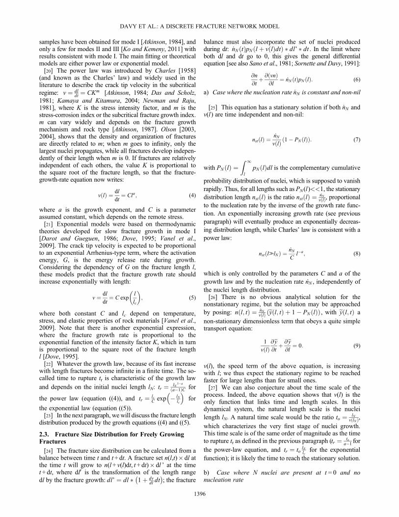
[36] As recalled in the “Introduction” section, the UFMrule imposes the arrest of fractures when they encounterlarger ones. Basically, a fracture propagates until it intersectslarger fractures. This rule is, however, not univocal since itmakes the fracture propagation vanish beyond such fractureintersections, but it does not tell anything about the fracturegrowth in other directions. We define different growth/stopmodels according to the number of degrees of freedom ofthe fracture growth. The first and basic degree of freedomis the fracture radius. A fracture that uniformly grows (indirections) from a fixed center has only one degree offreedom. Its growth will be stopped as soon as it intersects

Mode A Mode B

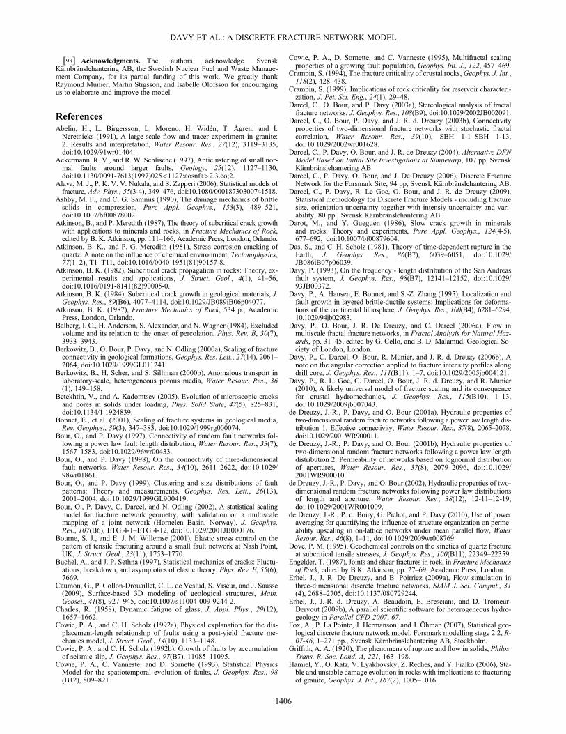
Figure 2. Illustration of the two different arrest rules.(Left) Mode A. (Right) Mode B. Fractures 2 and 3 are fixed.Fracture 1 is drawn at two different stages: light blue for thefirst stage where the fracture is still growing; dark blue forthe second stage corresponding to the point where fracturestops growing. See text for details.

DAVY ET AL.: A DISCRETE FRACTURE NETWORK MODEL

1397

the first larger fracture. We define this as the mode-A growthmodel (Figure 2, mode A).[37] An additional degree of freedom can be added by

allowing the fracture center to move if necessary (Figure 2,mode B). Let us assume that the growth rate of the fracture1 is inhibited by the intersection with a larger fracture 2.At this point, the fracture 1 is tangential to 2; it can continueto grow in all other directions as long it remains tangential to2. This can be achieved in different ways depending on thedistribution of fracture growth rate along the edge of fracture1. If we assume that fractures remain disk-shaped (uniformgrowth rate along the edge), there is only 1 additional degreeof freedom since the fracture center can only move along theline perpendicular to fracture 2 in order to maintain fracture1 tangential to fracture 2. This mode is further called mode-Bgrowth (Figure 2).[38] Additional degrees of freedom can be added by

relaxing the disk-shape hypothesis (e.g., truncated ellipses).In this paper, we only examine mode-A and mode-Bgrowth models.[39] For any mode of arrest, the UFM framework defined

in Davy et al. [2010] predicts that during the growth of afracture system, once mechanical interactions between frac-tures become dominant, a likely unique regime appears. Itis called the UFM “dense” regime to reflect that this regimeeffectively defines the densest possible values of fracturesize distribution.[40] In either mode A or mode B (Figure 2), the length of

the arrested fracture l is equal to twice the distance betweenthe fracture center and the closest larger fracture plane dP. Tocalculate the density distribution, we relate dP to the averagedistance between fracture centers d and assume that there isa dimensionless ratio g so that l= gd. With this assumption,the density distribution of the dense regime is:

ndense lð Þ ¼ DgDl� Dþ1ð Þ; (14)

with D the topological—either fractal or Euclidian—dimension associated to fracture centers [Davy et al., 2010]that can be calculated with box-counting methods. Thusdefined, g is a geometrical number related to local spatialconditions around fractures, that is, fracture orientationdistribution and also potentially fracture arrest mode.[41] The UFM dense regime is characterized by a self-

similar distribution, the length scaling exponent of whichis adense =D+ 1. The density term, DgD depends only onthe g parameter, the possible variations of which are furtherinvestigated in section 4.[42] Beyond the fracture length scaling, the UFM model

leads to specific fracture-to-fracture interactions and spatialorganization. The latter is reflected in the apparition of“T” fracture terminations in addition to classical “X”fracture intersections otherwise observed when fracturepositions are independently assigned (like in stochasticPoissonian models).

2.5. Combination of Nucleation, Growth, and Arrest

[43] When independently considered, both the dilute(freely growing fractures) and dense (stopped fractures)regimes have stationary density limits defined by equations

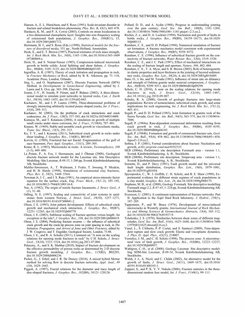
((8) (or ((11)) and ((14), respectively. The three mainregimes can be defined, as sketched in Figure 3: a regimepartly controlled by the nuclei distribution for the smallestlengths (part 1), a regime controlled by the growth law andnuclei rate (independently of the nuclei length probabilitydistribution) for intermediate lengths (part 2), the UFMdense regime for the largest fractures (part 3). The scalefor which both stationary density distributions are equal isgiven by:

lc ¼ DgD C

_nN

� � 1Dþ1�a

: (15)

[44] This general scheme should still be qualitatively validwhen considering the three main stages of fracturing (nucleation,growth, and arrest) but with important differences. Indeed,since the total number of fractures and of fracture lengthsis continuously increasing during the fracturing process(both by nucleation and fracture growth), the dense regimeshould spread towards smaller and smaller fractures—which is equivalent to say that arrested fractures becomesmaller and smaller. The combination of the stationarydensity equations ((8) (or ((11)) and ((14), although it is aninteresting reference, cannot define the stationary regime ofthe whole fracturing process.

2.6. Numerical Implementation

[45] We propose a 3D time-wise DFN generation methodbased on the above described theoretical model. It is developedwithin the software platform H2OLAB [de Dreuzy et al.,2010; Erhel et al., 2009a, b; Pichot et al., 2010]. Fracturesare modeled by disks and are embedded in a 3D polyhedron.[46] The fracture nucleation and propagation are

implemented following sections 2.1 to 2.3. In practice, a vir-tual time t is simulated, starting from t= 0 to the end of theprocess. This time line is divided in time steps Δt; for eachtime step, new fractures are generated (nucleation) and frac-ture propagation is applied.[47] At each time step, _nNΔt nuclei are generated. These nu-

clei are created at a time that is uniformly spread within thetime step, in order to better reproduce a continuous nucleation.[48] Fracture length is increased according to equation ((4),

which yields:

Figure 3. Illustration of the length distribution of the correlated3D-DFN models.

DAVY ET AL.: A DISCRETE FRACTURE NETWORK MODEL

1398

l t þ Δtð Þ ¼ l tð Þ1�a þ 1� að Þ�C�Δt� � 1

1�a: (16)

[49] The generation scheme is sketched below:

1) Initialization: t := 0

Then the dynamic process starts. It is composed as follow:

2) Set t := t + t

3) Nucleation stage:

define new nuclei

keep new nuclei only if no intersection with existing fractures,

4) Fracture growth stage - Eq. (16)

5) Computation of intersections

6) Fracture-length reduction according to mode A or mode B

7) Check ending criteria

If criteria are fulfilled, go to step 8),

else, return to step 2).

Finally, the generation is stopped:

8) Finalization, computation of intersections and statistics on the DFN.

[50] Note that the nuclei are not added in the system ifthey are arrested by the existing fracture network. The effec-tive nucleation rate is, thus, likely decreasing with time asthe space available for new nuclei is decreasing. This pointwill be discussed in the next paragraphs.[51] During one time step, a fracture may grow so that it

intersects more than one (in mode A) or two (in mode B)fractures. In such case, the intersected fractures are sortedaccording to their respective distance to the growing frac-tures and the arrest rule accordingly applied. The time stepis reduced to minimize such conflicts.[52] In practice, the DFN is generated in a cubic volume of

side L. Nucleation occurs only in the cube. Borders of thegeneration cube act as limits, beyond such fractures are notallowed to grow. No edge effects have been detected withthese rules mainly because the total surface of fractures israpidly much larger than the boundary surfaces, and thecontribution of the latter to stopping internal fracturesbecomes negligible.[53] In principle, the DFN can grow until there is no more

available space to put new nuclei or to propagate one frac-ture. Some ending criteria are defined:[54] 1. Nucleation is stopped when no nuclei can be added

in the system, and no fracture can grow anymore;[55] 2. Nucleation is stopped after a while, so as to obtain

a fixed length distribution;[56] 3. Nucleation is stopped when the targeted fracture

density is achieved.

3. Numerical Simulations of the DFN Model

[57] The model described in the previous paragraph is de-fined by a set of assumptions (Table 1) and parameters:p lð Þ; _nN tð Þ for nucleation; C, a for the growth law; modeA or B for the arrest condition. Length, density distribution,and time are given in an dimensionless form by normalizingwith the characteristic length lo and/or the characteristic timeto: t0 = t/t0, l0 = l/l0 , n0(l0) = n(l) * l0, pN0(l ’) = pN(l) * lo, and

_nN0t’ð Þ ¼ _nN tð Þ � to . The characteristic length scale lo is the

nuclei length lo = lN, and the time scale to is to ¼ lNv lNð Þ ¼

1ClN a�1, which is close to the time to rupture for nuclei of size lN.

3.1. Freely Growing Fracture Distribution

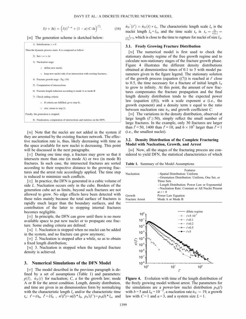
[58] The numerical model is first used to check thestationary density regime of the free growth regime and tocalculate non-stationary stages of the fracture growth phase.Figure 4 illustrates the different density distributionsobtained at dimensionless times of 0.1 to 5 with model pa-rameters given in the figure legend. The stationary solutionof the growth process (equation ((7)) is reached at t0 closeto 0.5, the time necessary for a fracture of initial length lNto grow to infinity. At this point, the amount of new frac-tures compensates the fracture propagation and the finallength density distribution tends to the expected powerlaw (equation ((8)), with a scale exponent a (i.e., thegrowth exponent) and a density term a equal to the ratiobetween nucleation rate _nN and growth coefficient C.[59] The variations in the density distribution, observed at

large length (l0 ≥ 50), simply reflect the small number oflarge fractures. In the example, only 30 fractures are largerthan l0 = 50, 1400 than l0 = 10, and 6� 105 larger than l0 = 1(i.e., the smallest nuclei).

3.2. Density Distribution of the Complete FracturingModel with Nucleation, Growth, and Arrest

[60] Now, all the stages of the fracturing process are con-sidered to yield DFN, the statistical characteristics of which

Table 1. Summary of the Model Assumptions

FeaturesNucleation �Spatial Distribution: Uniform

�Orientation Distribution: Uniform, One Set, orThree Sets�Length Distribution: Power Law or Exponential�Nucleation Rate: Constant or All Nuclei Presentat t = 0

Growth Power Law EquationFracture Arrest Mode A or Mode B

100 101 10210-8

10-7

10-6

10-5

10-4

10-3

10-2

10-1

100

n'( l

')

l'

dilute regime

t'=5·10-3

t'=0.1t'=0.2t'=0.5t'=5

Figure 4. Evolution with time of the length distribution ofthe freely growing model without arrest. The parameters forthe simulations are a power-law nuclei distribution pN(l )with b = 5 and lN = 10

�2, a nucleation rate _nN ¼ 19, a growthlaw with C= 1 and a= 3, and a system size L= 1.

DAVY ET AL.: A DISCRETE FRACTURE NETWORK MODEL

1399

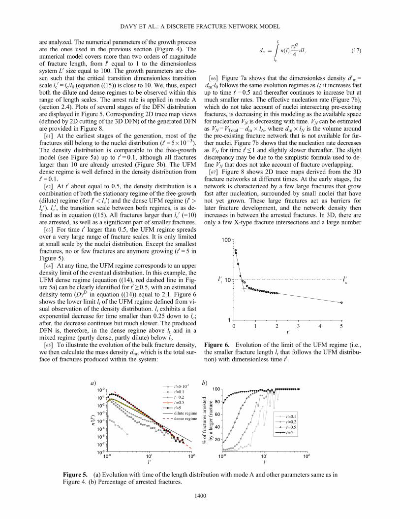
are analyzed. The numerical parameters of the growth processare the ones used in the previous section (Figure 4). Thenumerical model covers more than two orders of magnitudeof fracture length, from l0 equal to 1 to the dimensionlesssystem L0 size equal to 100. The growth parameters are cho-sen such that the critical transition dimensionless transitionscale lc0 = lc/l0 (equation ((15)) is close to 10. We, thus, expectboth the dilute and dense regimes to be observed within thisrange of length scales. The arrest rule is applied in mode A(section 2.4). Plots of several stages of the DFN distributionare displayed in Figure 5. Corresponding 2D trace map views(defined by 2D cutting of the 3D DFN) of the generated DFNare provided in Figure 8.[61] At the earliest stages of the generation, most of the

fractures still belong to the nuclei distribution (t0 = 5�10�3).The density distribution is comparable to the free-growthmodel (see Figure 5a) up to t0 = 0.1, although all fractureslarger than 10 are already arrested (Figure 5b). The UFMdense regime is well defined in the density distribution fromt0 = 0.1.[62] At t0 about equal to 0.5, the density distribution is a

combination of both the stationary regime of the free-growth(dilute) regime (for l0 < lc0) and the dense UFM regime (l0 >lc0). lc0, the transition scale between both regimes, is as de-fined as in equation ((15). All fractures larger than lc0 (=10)are arrested, as well as a significant part of smaller fractures.[63] For time t0 larger than 0.5, the UFM regime spreads

over a very large range of fracture scales. It is only limitedat small scale by the nuclei distribution. Except the smallestfractures, no or few fractures are anymore growing (t0 = 5 inFigure 5).[64] At any time, the UFM regime corresponds to an upper

density limit of the eventual distribution. In this example, theUFM dense regime (equation ((14), red dashed line in Fig-ure 5a) can be clearly identified for t0 ≥ 0.5, with an estimateddensity term (DgD in equation ((14)) equal to 2.1. Figure 6shows the lower limit lt of the UFM regime defined from vi-sual observation of the density distribution. lt exhibits a fastexponential decrease for time smaller than 0.25 down to lc;after, the decrease continues but much slower. The producedDFN is, therefore, in the dense regime above lt and in amixed regime (partly dense, partly dilute) below lt.[65] To illustrate the evolution of the bulk fracture density,

we then calculate the mass density dm, which is the total sur-face of fractures produced within the system:

dm ¼ZLl0

n lð Þ pl2

4dl; (17)

[66] Figure 7a shows that the dimensionless density d0m=dm�l0 follows the same evolution regimes as lt: it increases fastup to time t0 =0.5 and thereafter continues to increase but atmuch smaller rates. The effective nucleation rate (Figure 7b),which do not take account of nuclei intersecting pre-existingfractures, is decreasing in this modeling as the available spacefor nucleation VN is decreasing with time. VN can be estimatedas VN=VTotal� dm� lN, where dm� lN is the volume aroundthe pre-existing fracture network that is not available for fur-ther nuclei. Figure 7b shows that the nucleation rate decreasesas VN for time t0 ≤ 1 and slightly slower thereafter. The slightdiscrepancy may be due to the simplistic formula used to de-fine VN that does not take account of fracture overlapping.[67] Figure 8 shows 2D trace maps derived from the 3D

fracture networks at different times. At the early stages, thenetwork is characterized by a few large fractures that growfast after nucleation, surrounded by small nuclei that havenot yet grown. These large fractures act as barriers forlater fracture development, and the network density thenincreases in between the arrested fractures. In 3D, there areonly a few X-type fracture intersections and a large number

a) b)

10-8

10-7

10-6

10-5

10-4

10-3

10-2

10-1

10-0

10-0 101 102 10-0 101 102

n'(l

')

l'

t'=5·10-3

t'=0.1t'=0.2t'=0.5t'=5 dilute regime dense regime

20

40

60

80

100

% o

f fr

actu

res

arre

sted

by a

larg

er f

ract

ure

l'

t'=0.1t'=0.2t'=0.5t'=5

Figure 5. (a) Evolution with time of the length distribution with mode A and other parameters same as inFigure 4. (b) Percentage of arrested fractures.

0 1 2 3 4 51

10

100

l't

t'

l'c

Figure 6. Evolution of the limit of the UFM regime (i.e.,the smaller fracture length lt that follows the UFM distribu-tion) with dimensionless time t0.

DAVY ET AL.: A DISCRETE FRACTURE NETWORK MODEL

1400

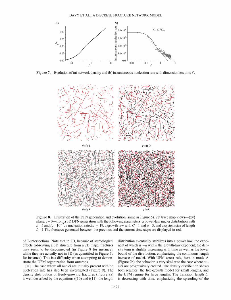
of T-intersections. Note that in 2D, because of stereologicaleffects (observing a 3D structure from a 2D map), fracturesmay seem to be disconnected (in Figure 8 for instance),while they are actually not in 3D (as quantified in Figure 5bfor instance). This is a difficulty when attempting to demon-strate the UFM organization from outcrops.[68] The case where all nuclei are initially present with no

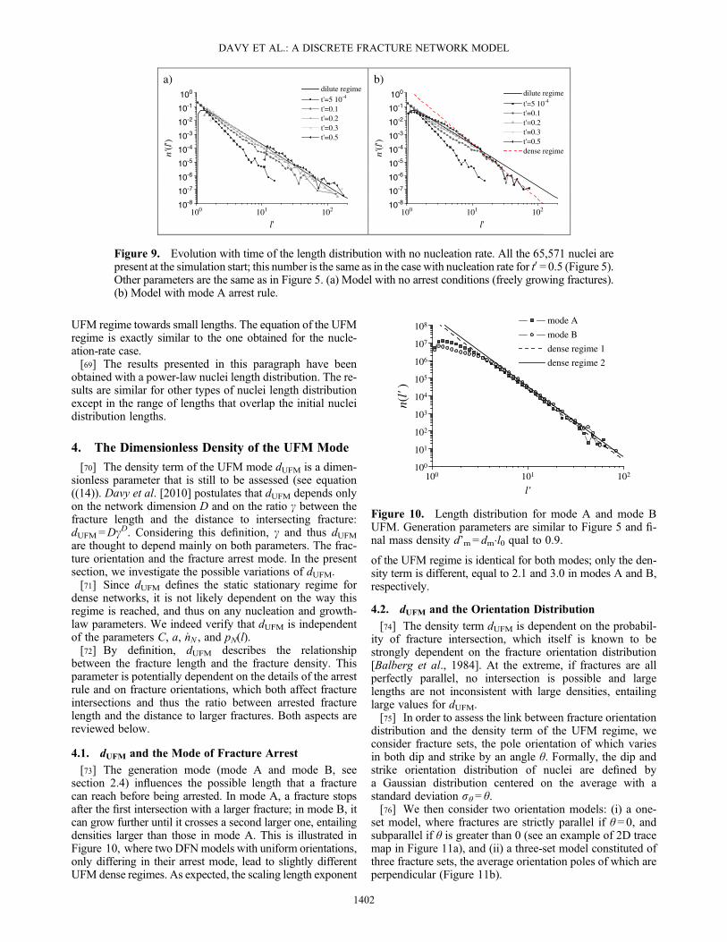
nucleation rate has also been investigated (Figure 9). Thedensity distribution of freely-growing fractures (Figure 9a)is well described by the equations ((10) and ((11): the length

distribution eventually stabilizes into a power law, the expo-nent of which is�a with a the growth-law exponent; the den-sity term is slightly increasing with time as well as the lowerbound of the distribution, emphasizing the continuous lengthincrease of nuclei. With UFM arrest rule, here in mode A(Figure 9b), the behavior is very similar to the case where nu-clei are progressively created. The density distribution showsboth regimes: the free-growth model for small lengths, andthe UFM regime for large lengths. The transition length lc0is decreasing with time, emphasizing the spreading of the

Figure 8. Illustration of the DFN generation and evolution (same as Figure 5). 2D trace map views—(xy)plane, z=0—from a 3DDFN generation with the following parameters: a power-law nuclei distribution withb= 5 and lN=10

�2, a nucleation rate _nN ¼ 19, a growth law with C=1 and a=3, and a system size of lengthL=1.The fractures generated between the previous and the current time steps are displayed in red.

a) b)

0.1 1 100.00

0.25

0.50

0.75

1.00

d'm

t'0.01 0.1 1 10

0.0

5.0x104

1.0x105

1.5x105

2.0x105

inst

anta

neou

s nu

clea

tion

rate

t'

' ' 'N N totaln V V

Figure 7. Evolution of (a) network density and (b) instantaneous nucleation rate with dimensionless time t 0.

DAVY ET AL.: A DISCRETE FRACTURE NETWORK MODEL

1401

UFM regime towards small lengths. The equation of the UFMregime is exactly similar to the one obtained for the nucle-ation-rate case.[69] The results presented in this paragraph have been

obtained with a power-law nuclei length distribution. The re-sults are similar for other types of nuclei length distributionexcept in the range of lengths that overlap the initial nucleidistribution lengths.

4. The Dimensionless Density of the UFM Mode

[70] The density term of the UFM mode dUFM is a dimen-sionless parameter that is still to be assessed (see equation((14)). Davy et al. [2010] postulates that dUFM depends onlyon the network dimension D and on the ratio g between thefracture length and the distance to intersecting fracture:dUFM=DgD. Considering this definition, g and thus dUFMare thought to depend mainly on both parameters. The frac-ture orientation and the fracture arrest mode. In the presentsection, we investigate the possible variations of dUFM.[71] Since dUFM defines the static stationary regime for

dense networks, it is not likely dependent on the way thisregime is reached, and thus on any nucleation and growth-law parameters. We indeed verify that dUFM is independentof the parameters C, a, _nN , and pN(l).[72] By definition, dUFM describes the relationship

between the fracture length and the fracture density. Thisparameter is potentially dependent on the details of the arrestrule and on fracture orientations, which both affect fractureintersections and thus the ratio between arrested fracturelength and the distance to larger fractures. Both aspects arereviewed below.

4.1. dUFM and the Mode of Fracture Arrest

[73] The generation mode (mode A and mode B, seesection 2.4) influences the possible length that a fracturecan reach before being arrested. In mode A, a fracture stopsafter the first intersection with a larger fracture; in mode B, itcan grow further until it crosses a second larger one, entailingdensities larger than those in mode A. This is illustrated inFigure 10, where two DFNmodels with uniform orientations,only differing in their arrest mode, lead to slightly differentUFM dense regimes. As expected, the scaling length exponent

of the UFM regime is identical for both modes; only the den-sity term is different, equal to 2.1 and 3.0 in modes A and B,respectively.

4.2. dUFM and the Orientation Distribution

[74] The density term dUFM is dependent on the probabil-ity of fracture intersection, which itself is known to bestrongly dependent on the fracture orientation distribution[Balberg et al., 1984]. At the extreme, if fractures are allperfectly parallel, no intersection is possible and largelengths are not inconsistent with large densities, entailinglarge values for dUFM.[75] In order to assess the link between fracture orientation

distribution and the density term of the UFM regime, weconsider fracture sets, the pole orientation of which variesin both dip and strike by an angle θ. Formally, the dip andstrike orientation distribution of nuclei are defined bya Gaussian distribution centered on the average with astandard deviation sθ= θ.[76] We then consider two orientation models: (i) a one-

set model, where fractures are strictly parallel if θ= 0, andsubparallel if θ is greater than 0 (see an example of 2D tracemap in Figure 11a), and (ii) a three-set model constituted ofthree fracture sets, the average orientation poles of which areperpendicular (Figure 11b).

a) b)

100 101 102

10-1

10-2

10-3

10-4

10-5

10-6

10-7

10-8

100 dilute regime t'=5 10-4

t'=0.1 t'=0.2 t'=0.3 t'=0.5

n'(l

')

10-1

10-2

10-3

10-4

10-5

10-6

10-7

10-8

100

n'(l

')

l'100 101 102

l'

dilute regime t'=5 10-4

t'=0.1 t'=0.2 t'=0.3 t'=0.5 dense regime

Figure 9. Evolution with time of the length distribution with no nucleation rate. All the 65,571 nuclei arepresent at the simulation start; this number is the same as in the case with nucleation rate for t0 =0.5 (Figure 5).Other parameters are the same as in Figure 5. (a) Model with no arrest conditions (freely growing fractures).(b) Model with mode A arrest rule.

108

107

106

105

104

103

102

101

100

100 101 102

mode A

mode B

dense regime 1

dense regime 2

n(l'

)

l'

Figure 10. Length distribution for mode A and mode BUFM. Generation parameters are similar to Figure 5 and fi-nal mass density d’m= dm�l0 qual to 0.9.

DAVY ET AL.: A DISCRETE FRACTURE NETWORK MODEL

1402

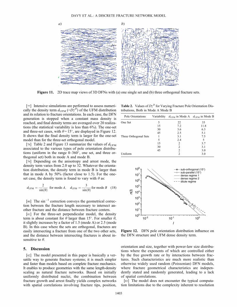
[77] Intensive simulations are performed to assess numeri-cally the density term dUFM (=DgD) of the UFM distributionand its relation to fracture orientations. In each case, the DFNgeneration is stopped when a constant mass density isreached, and final density terms are averaged over 20 realiza-tions (the statistical variability is less than 6%). The one-setand three-set cases, with θ= 15�, are displayed in Figure 12.It shows that the final density term is larger for the one-setmodel than for the three-set orthogonal model.[78] Table 2 and Figure 13 summarize the values of dUFM

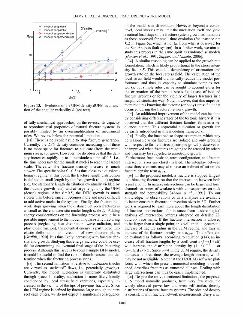
associated to the various types of pole orientation distribu-tions (uniform in the range 0–360�, one set, and three or-thogonal set) both in mode A and mode B.[79] Depending on the anisotropy and arrest mode, the

density term varies from 2.0 up to 32. Whatever the orienta-tion distribution, the density term in mode B is larger thanthat in mode A by 50% (factor close to 1.5). For the one-set case, the density term is found to vary with θ as:

dUFM ¼ 2

sin θð Þ for mode A; dUFM ¼ 3

sin θð Þ for mode B (18)

[80] The sin�1 correction conveys the geometrical correc-tion between the fracture length necessary to intersect an-other fracture and the distance between fracture centers.[81] For the three-set perpendicular model, the density

term is about constant for θ larger than 15�. For smaller θ,it slightly increases by a factor of 1.5 (mode A) or 2.5 (modeB). In this case where the sets are orthogonal, fractures areeasily intersecting a fracture from one of the two other sets,and the distance between intersecting fractures is about in-sensitive to θ.

5. Discussion

[82] The model presented in this paper is basically a ver-satile way to generate fracture systems; it is much simplerand faster than models based on complete fracture mechanics.It enables to produce geometries with the same length-densityscaling as natural fracture networks. Based on initiallyuniformly distributed nuclei, the combination betweenfracture growth and arrest finally yields complex networkswith spatial correlations involving fracture tips, position,

orientation and size, together with power-law size distribu-tions where the exponents of which are controlled eitherby the free growth rate or by interactions between frac-tures. Such characteristics are much more realistic thanotherwise widely used random (Poissonian) DFN models,where fracture geometrical characteristics are indepen-dently stated and randomly generated, leading to a lackof spatial correlations.[83] The model does not encounter the typical computa-

tion limitations due to the complexity inherent to resolution

a) b)

Figure 11. 2D trace map views of 3D DFNs with (a) one single set and (b) three orthogonal fracture sets.

10-2 10-1 100

108

107

106

105

104

103

102

101

100

n(l)

l

sub-orthogonal (15°)sub-parallel (15°)dense regime 1dense regime 2dilute regime

Figure 12. DFN pole orientation distribution influence onthe DFN structure and UFM dense density term.

Table 2. Values of DgD for Varying Fracture Pole Orientation Dis-tributions, Both in Mode A Mode B

Pole Orientations Variability dUFM in Mode A dUFM in Mode B

One Set 5 22 3315 7.2 11.830 3.6 6.345 2.5 5.1

Three Orthogonal Sets 1 3.1 7.55 2.4 515 2 3.730 2 3.145 2 3.0

Uniform 2 3.0

DAVY ET AL.: A DISCRETE FRACTURE NETWORK MODEL

1403

of fully mechanical approaches; on the reverse, its capacityto reproduce real properties of natural fracture systems ispossibly limited by an oversimplification of mechanicalrules. We review below the potential limitations.[84] There is no explicit rule to stop fracture generation.

Currently, the DFN density continues increasing until thereis no more space for fractures to nucleate (from the mini-mum size lN) or grow. However, we do observe that the den-sity increases rapidly up to dimensionless time of 0.5, i.e.,the time necessary for the smallest nuclei to reach the largestscale. Thereafter the fracture density increase is muchslower. The specific point t0 ~ 0.5 is thus close to a quasi-sta-tionary regime; at this point, the fracture length distributionis defined at small length by the free-growth (dilute) regime(i.e., the stationary length distribution eventually yielded bythe fracture growth law), and at large lengths by the UFM(dense) regime. After t0 = 0.5, the DFN growth is muchslower than before, since it becomes more and more difficultto add active nuclei in the system. Finally, the fracture net-work stops growing when the distance between fractures isas small as the characteristic nuclei length scale lN. Addingenergy considerations on the fracturing process would be apossible improvement to the model. In quasi-static fracturingprocess (neglecting heat dissipation, wave radiation, andplastic deformation), the potential energy is partitioned intoelastic deformation and creation of new fracture planes[Griffith, 1920]. It is thus likely increasing with fracture den-sity and growth. Studying this energy increase could be use-ful for determining the eventual final stage of the fracturingprocess. Although this issue is beyond a simple DFN model,it could be useful to find the rule-of-thumb reasons that de-termine when the fracturing process stops.[85] The second limitation is relative to nucleation (nuclei

are viewed as “activated” flaws, i.e., potentially growing).Currently, the model nucleation is uniformly distributedthrough space. In reality, nucleation is more likely locallyconditioned by local stress field variations, especially in-creased in the vicinity of the tips of previous fractures. Sincethe UFM regime is defined by fractures large enough to inter-sect each others, we do not expect a significant consequence

on the model size distribution. However, beyond a certainlevel, local stresses may limit the nucleation itself and yielda natural final stage of the fracture system growth as immatureas those observed for small time evolution (for instance t0 =0.2 in Figure 5a, which is not far from what is observed forthe San Andreas fault system). In a further work, we aim tostudy this process in the same spirit as random-fuse models[Hansen et al., 1991; Zapperi and Nukala, 2006].[86] A similar reasoning can be applied to the growth rate

formulation, which is likely proportional to the stress inten-sity factor K. This entails a dependency of orientation andgrowth rate on the local stress field. The calculation of thelocal stress field would dramatically reduce the model per-formance and thus its capacity to simulate complex net-works, but simple rules can be sought to account either forthe orientation of the remote stress field (case of isolatedfracture growth) or for the vicinity of larger fractures in asimplified stochastic way. Note, however, that this improve-ment requires knowing the tectonic (or body) stress field thatoccurred during the fracture network growth.[87] An additional improvement of the model can be done

by considering different stages of the tectonic history if it isobserved that the different fracture families form as a se-quence in time. This sequential nucleation or growth canbe easily introduced in this modeling framework.[88] Finally, the fracture disc-shape assumption, which may

be reasonable when fractures are isolated and only growingwith respect to far field stress (isotropic growth), deserves tobe improved when fractures are going to be arrested by othersand then may be subjected to anisotropic growth.Furthermore, fracture shape, arrest configuration, and fractureintersection sizes are closely related. The interplay betweenthese three elements may also have an indirect effect on thefracture density term dUFM.[89] In the proposed model, a fracture is stopped tangent

to a blocking fracture, so that the intersection between bothis just a point. In nature, intersections can be larger and formchannels or zones of weakness with consequences on rockstrength and permeability [Abelin et al., 1991]. To ourknowledge, no observations or data analyses are availableto better constrain fracture intersection sizes in 3D. Furtherwork is required to learn more about the length distributionof fracture intersections, for instance from a stereologicalanalysis of intersection patterns observed on detailed 2Doutcrop trace maps. If the fracture intersection is allowedto be larger than a single point, this will entail a systematicincrease of fracture radius in the UFM regime, and thus anincrease of the fracture density term dUFM. This effect canbe evaluated as follows: according to equation ((14), an in-crease of all fracture lengths by a coefficient e (l0 = (1 + e)l)will increase the distribution density by (1 + e)a� 1�1 or(a�1)e if e<<1. Since a = 4 in the UFM regime, the densityincreases is three times the average length increase, whichmay be not negligible. Note that the H2OLAB software plat-form, with which the present numerical modeling is devel-oped, describes fractures as truncated ellipses. Dealing withlarge intersections can thus be easily implemented.[90] Despite the above mentioned limitations, the proposed

DFN model naturally produces, from very few rules, thewidely observed power-law and even self-similar, densitydistributions of natural fracture systems. The obtained densityis consistent with fracture network measurements. Davy et al.

mode A subparallelmode B subparallelmode A subperpendicularmode B subperpendicular

1 101

10

7

3

2

2*sin(θ)-13*sin(θ)-1

sin(θ)-1

UFM

Figure 13. Evolution of the UFM density dUFM as a func-tion of the angular variability θ (see text).

DAVY ET AL.: A DISCRETE FRACTURE NETWORK MODEL

1404

[2010] has shown that the scaling and density of the UFMmodel is consistent with different kinds of fracture systems:joint and fault systems in different places of Norway(Hornelen basin [Bour et al., 2002; Odling, 1997]), of Swe-den (Forsmark, Simpevarp, and Laxemar [Darcel et al.,2004; Darcel et al., 2009; Fox et al., 2007; La Pointe et al.,2008; SKB, 2004b; Stephens et al., 2008; Wahlgren et al.,2008]), and of the San Andreas fault system [Bour and Davy,1999; Davy, 1993]. Most of the observations on natural frac-ture systems were made from 2D outcrop mapping, for whichthe density terms of the length density distribution was calcu-lated [Davy et al., 2010]. For Sweden and Norway joint sys-tems, the UFM regime is well defined above 3–5m, withthe expected 2D power-law length exponent of 3 and an ap-parent 2D density term varying between 2.2 to 4.5. The 3D-equivalent density, calculated by applying stereological rules[Davy et al., 2006b; Piggott, 1997], has been found to varybetween 3 and 5.5 (indicated by a grey-shaded rectangle inFigure 13 of Davy et al. [2010]) for the Simpevarp [Darcelet al., 2004] and Forsmark sites [Darcel et al., 2006]. Thisrange is consistent with both arrest modes A and B, as longas the orientation variability (equivalent to θ in the previousparagraph) is larger than 20�–30�. Such range of orientationanisotropy is currently observed on borehole logs and outcropmaps. No similar 3D analysis has yet been performed for theHornelen basin and San Andreas fault system. A more thor-ough analysis will require a complete stereological analysisfor each borehole log and outcrop map. This is beyond thescope of the present study. This work is, however, startingas part of continuing investigations conducted by the SKBCompany at the Äspö HRL and Forsmark sites.[91] Because of its particular spatial correlations and inter-

section properties, the application of the present frameworkto flow and mechanical modeling may end up in new rela-tions between DFN geometrical properties (density, scale)and consecutive flow or mechanical properties. This is likelyto have consequences on flow as illustrated in the very firstcalculations presented in Davy et al. [2010]. Another geo-metrical characteristic of the DFN produced with this modelis that the transition length lc between the dilute and dense/UFM regimes is actually a characteristic block size forunfractured domains. Fractures smaller than lc are poorlyconnected, and thus hardly define blocks in 3D. In theUFM regime (fracture length larger than lc), fractures forman interconnected network, the distance of which betweenfractures is about lc. This block size is a critical parameterfor any mechanical study of rock mass (see for instance[Hoek and Brown, 1997]).[92] The promising capacity of the UFM model to reflect

geometrical observations finally reinforces the potential ofthis model to be also relevant for modeling flow and me-chanical applications of natural systems. Moreover, theUFM length distribution, the scaling properties of whichare fully defined, fixes an upper limit of any fracture size dis-tribution model that cannot be bypassed. Such characteristicstrongly reduces uncertainty in the DFN modeling.

6. Conclusion

[93] In this paper, we aim to improve stochastic DFNmodels by developing a method which reproduces the mainstages of fracture evolution while preserving the currently

observed scaling characteristics. The model combines, in atime-wise process, a spatially uniform nucleation offractures, a power-law model of fracture growth and agrowth arrest rule when fracture intersects another largerone. The latter aspect was firstly described in Davy et al.[2010]. Thus defined, the generation process naturally cre-ates internal spatial correlations, together with multiscalefracture size distributions, producing statistical propertiesthat are equivalent to those of real fracture systems.[94] The statistical properties of produced DFNs were an-

alyzed by calculating the density distribution of fracturelength n(l), which describes the relationship between frac-ture length and density. n(l) can be divided in three regions:for small lengths, it is mainly controlled by the size distribu-tion of nuclei; for intermediate lengths, it depends on boththe fracture growth law and nucleation rate, converging toa well-defined power law with a scaling exponent equal tominus the growth rate exponent. At large lengths, n(l) con-verges to the self-similar UFM regime defined in Davyet al. [2010], where the scaling exponent is �(D+ 1), withD the (possibly fractal) topological dimension of the net-work centres. The dimensionless density term, dUFM, is afunction of the fracture (thus nuclei) orientation distribution,and of the details of the arrest rule.[95] The relative importance of the three above-mentioned

regimes evolves throughout the generation process. At earli-est times, most of the fractures belong to the initial nucleisize distribution. The total fracture mass (i.e., sum of fractureareas) is growing at constant rate up to the time necessaryfor the smallest nuclei to reach the largest scale. At this inter-mediate stage, for which no fracture can grow freely anymore,n(l) follows both the stationary free-growing regime and thedense/UFM, respectively, below and above a transitionscale. After that time, if more nuclei are activated, the frac-ture mass goes on increasing (but at a much slower rate),and the UFM/dense regime tends to spread toward smallerand smaller fracture lengths.[96] The UFM/dense regime is the most striking feature of

produced DFN. While fractures are growing, it spreads outfrom the largest length (about the system size) to smallerand smaller lengths. The scaling exponent is uniquely de-fined, but the density term depends on the mode of arrest(factor 2/3 between mode A and mode B) and on theeventual fracture orientation distribution. The UFM densitydistribution is in good accordance with several field cases(especially for the Laxemar and Forsmark sites in Swedenand Hornelen basin in Norway). Finally, this model stronglyreduces uncertainties inherent to any DFN modeling exer-cise. The UFM regime is also an upper limit of any fracturelength distribution where T-intersections prevail (whichseems to be the general rule in fracture systems). This bringsan interesting constrain to any DFN modeling.[97] Improving DFN modeling is of primary importance to

improve flow and mechanical modeling of underground sys-tems, especially in a context where data are very scarce withregard to the fracture network complexity. Identifying somebasic rules of fracture organization as we do in this paper isan interesting way to come closer to geological complexity.The good adequacy of the UFM model with simplified me-chanical rules and with field data observations reinforces thepotential of this model to be also relevant for the applicationto flow and mechanical modeling of natural fractured systems.

DAVY ET AL.: A DISCRETE FRACTURE NETWORK MODEL

1405

[98] Acknowledgments. The authors acknowledge SvenskKärnbränslehantering AB, the Swedish Nuclear Fuel and Waste Manage-ment Company, for its partial funding of this work. We greatly thankRaymond Munier, Martin Stigsson, and Isabelle Olofsson for encouragingus to elaborate and improve the model.

ReferencesAbelin, H., L. Birgersson, L. Moreno, H. Widén, T. Ågren, and I.Neretnieks (1991), A large-scale flow and tracer experiment in granite:2. Results and interpretation, Water Resour. Res., 27(12), 3119–3135,doi:10.1029/91wr01404.

Ackermann, R. V., and R. W. Schlische (1997), Anticlustering of small nor-mal faults around larger faults, Geology, 25(12), 1127–1130,doi:10.1130/0091-7613(1997)025<1127:aosnfa>2.3.co;2.

Alava, M. J., P. K. V. V. Nukala, and S. Zapperi (2006), Statistical models offracture, Adv. Phys., 55(3-4), 349–476, doi:10.1080/00018730300741518.

Ashby, M. F., and C. G. Sammis (1990), The damage mechanics of brittlesolids in compression, Pure Appl. Geophys., 133(3), 489–521,doi:10.1007/bf00878002.

Atkinson, B., and P. Meredith (1987), The theory of subcritical crack growthwith applications to minerals and rocks, in Fracture Mechanics of Rock,edited by B. K. Atkinson, pp. 111–166, Academic Press, London, Orlando.

Atkinson, B. K., and P. G. Meredith (1981), Stress corrosion cracking ofquartz: A note on the influence of chemical environment, Tectonophysics,77(1–2), T1–T11, doi:10.1016/0040-1951(81)90157-8.

Atkinson, B. K. (1982), Subcritical crack propagation in rocks: Theory, ex-perimental results and applications, J. Struct. Geol., 4(1), 41–56,doi:10.1016/0191-8141(82)90005-0.

Atkinson, B. K. (1984), Subcritical crack growth in geological materials, J.Geophys. Res., 89(B6), 4077–4114, doi:10.1029/JB089iB06p04077.

Atkinson, B. K. (1987), Fracture Mechanics of Rock, 534 p., AcademicPress, London, Orlando.

Balberg, I. C., H. Anderson, S. Alexander, and N. Wagner (1984), Excludedvolume and its relation to the onset of percolation, Phys. Rev. B, 30(7),3933–3943.

Berkowitz, B., O. Bour, P. Davy, and N. Odling (2000a), Scaling of fractureconnectivity in geological formations, Geophys. Res. Lett., 27(14), 2061–2064, doi:10.1029/1999GL011241.

Berkowitz, B., H. Scher, and S. Silliman (2000b), Anomalous transport inlaboratory-scale, heterogeneous porous media, Water Resour. Res., 36(1), 149–158.

Betekhtin, V., and A. Kadomtsev (2005), Evolution of microscopic cracksand pores in solids under loading, Phys. Solid State, 47(5), 825–831,doi:10.1134/1.1924839.

Bonnet, E., et al. (2001), Scaling of fracture systems in geological media,Rev. Geophys., 39(3), 347–383, doi:10.1029/1999rg000074.

Bour, O., and P. Davy (1997), Connectivity of random fault networks fol-lowing a power law fault length distribution, Water Resour. Res., 33(7),1567–1583, doi:10.1029/96wr00433.

Bour, O., and P. Davy (1998), On the connectivity of three-dimensionalfault networks, Water Resour. Res., 34(10), 2611–2622, doi:10.1029/98wr01861.

Bour, O., and P. Davy (1999), Clustering and size distributions of faultpatterns: Theory and measurements, Geophys. Res. Lett., 26(13),2001–2004, doi:10.1029/1999GL900419.

Bour, O., P. Davy, C. Darcel, and N. Odling (2002), A statistical scalingmodel for fracture network geometry, with validation on a multiscalemapping of a joint network (Hornelen Basin, Norway), J. Geophys.Res., 107(B6), ETG 4-1–ETG 4-12, doi:10.1029/2001JB000176.

Bourne, S. J., and E. J. M. Willemse (2001), Elastic stress control on thepattern of tensile fracturing around a small fault network at Nash Point,UK, J. Struct. Geol., 23(11), 1753–1770.

Buchel, A., and J. P. Sethna (1997), Statistical mechanics of cracks: Fluctu-ations, breakdown, and asymptotics of elastic theory, Phys. Rev. E, 55(6),7669.

Caumon, G., P. Collon-Drouaillet, C. L. de Veslud, S. Viseur, and J. Sausse(2009), Surface-based 3D modeling of geological structures, Math.Geosci., 41(8), 927–945, doi:10.1007/s11004-009-9244-2.

Charles, R. (1958), Dynamic fatigue of glass, J. Appl. Phys., 29(12),1657–1662.

Cowie, P. A., and C. H. Scholz (1992a), Physical explanation for the dis-placement-length relationship of faults using a post-yield fracture me-chanics model, J. Struct. Geol., 14(10), 1133–1148.

Cowie, P. A., and C. H. Scholz (1992b), Growth of faults by accumulationof seismic slip, J. Geophys. Res., 97(B7), 11085–11095.

Cowie, P. A., C. Vanneste, and D. Sornette (1993), Statistical PhysicsModel for the spatiotemporal evolution of faults, J. Geophys. Res., 98(B12), 809–821.

Cowie, P. A., D. Sornette, and C. Vanneste (1995), Multifractal scalingproperties of a growing fault population, Geophys. Int. J., 122, 457–469.

Crampin, S. (1994), The fracture criticality of crustal rocks, Geophys. J. Int.,118(2), 428–438.

Crampin, S. (1999), Implications of rock criticality for reservoir characteri-zation, J. Pet. Sci. Eng., 24(1), 29–48.

Darcel, C., O. Bour, and P. Davy (2003a), Stereological analysis of fractalfracture networks, J. Geophys. Res., 108(B9), doi:10.1029/2002JB002091.

Darcel, C., O. Bour, P. Davy, and J. R. d. Dreuzy (2003b), Connectivityproperties of two-dimensional fracture networks with stochastic fractalcorrelation, Water Resour. Res., 39(10), SBH 1-1–SBH 1-13,doi:10.1029/2002wr001628.

Darcel, C., P. Davy, O. Bour, and J. R. de Dreuzy (2004), Alternative DFNModel Based on Initial Site Investigations at Simpevarp, 107 pp, SvenskKärnbränslehantering AB.

Darcel, C., P. Davy, O. Bour, and J. De Dreuzy (2006), Discrete FractureNetwork for the Forsmark Site, 94 pp, Svensk Kärnbränslehantering AB.

Darcel, C., P. Davy, R. Le Goc, O. Bour, and J. R. de Dreuzy (2009),Statistical methodology for Discrete Fracture Models - including fracturesize, orientation uncertainty together with intensiy uncertainty and vari-ability, 80 pp., Svensk Kärnbränslehantering AB.

Darot, M., and Y. Gueguen (1986), Slow crack growth in mineralsand rocks: Theory and experiments, Pure Appl. Geophys., 124(4-5),677–692, doi:10.1007/bf00879604.

Das, S., and C. H. Scholz (1981), Theory of time-dependent rupture in theEarth, J. Geophys. Res., 86(B7), 6039–6051, doi:10.1029/JB086iB07p06039.

Davy, P. (1993), On the frequency - length distribution of the San Andreasfault system, J. Geophys. Res., 98(B7), 12141–12152, doi:10.1029/93JB00372.

Davy, P., A. Hansen, E. Bonnet, and S.-Z. Zhang (1995), Localization andfault growth in layered brittle-ductile systems: Implications for deforma-tions of the continental lithosphere, J. Geophys. Res., 100(B4), 6281–6294,10.1029/94jb02983.

Davy, P., O. Bour, J. R. De Dreuzy, and C. Darcel (2006a), Flow inmultiscale fractal fracture networks, in Fractal Analysis for Natural Haz-ards, pp. 31–45, edited by G. Cello, and B. D. Malamud, Geological So-ciety of London, London.

Davy, P., C. Darcel, O. Bour, R. Munier, and J. R. d. Dreuzy (2006b), Anote on the angular correction applied to fracture intensity profiles alongdrill core, J. Geophys. Res., 111(B11), 1–7, doi:10.1029/2005jb004121.

Davy, P., R. L. Goc, C. Darcel, O. Bour, J. R. d. Dreuzy, and R. Munier(2010), A likely universal model of fracture scaling and its consequencefor crustal hydromechanics, J. Geophys. Res., 115(B10), 1–13,doi:10.1029/2009jb007043.

de Dreuzy, J.-R., P. Davy, and O. Bour (2001a), Hydraulic properties oftwo-dimensional random fracture networks following a power law length dis-tribution 1. Effective connectivity, Water Resour. Res., 37(8), 2065–2078,doi:10.1029/2001WR900011.

de Dreuzy, J.-R., P. Davy, and O. Bour (2001b), Hydraulic properties oftwo-dimensional random fracture networks following a power law lengthdistribution 2. Permeability of networks based on lognormal distributionof apertures, Water Resour. Res., 37(8), 2079–2096, doi:10.1029/2001WR900010.

de Dreuzy, J.-R., P. Davy, and O. Bour (2002), Hydraulic properties of two-dimensional random fracture networks following power law distributionsof length and aperture, Water Resour. Res., 38(12), 12-11–12-19,doi:10.1029/2001WR001009.

de Dreuzy, J.-R., P. d. Boiry, G. Pichot, and P. Davy (2010), Use of poweraveraging for quantifying the influence of structure organization on perme-ability upscaling in on-lattice networks under mean parallel flow, WaterResour. Res., 46(8), 1–11, doi:10.1029/2009wr008769.

Dove, P. M. (1995), Geochemical controls on the kinetics of quartz fractureat subcritical tensile stresses, J. Geophys. Res., 100(B11), 22349–22359.

Engelder, T. (1987), Joints and shear fractures in rock, in Fracture Mechanicsof Rock, edited by B.K. Atkinson, pp. 27–69, Academic Press, London.

Erhel, J., J. R. De Dreuzy, and B. Poirriez (2009a), Flow simulation inthree-dimensional discrete fracture networks, SIAM J. Sci. Comput., 31(4), 2688–2705, doi:10.1137/080729244.

Erhel, J., J.-R. d. Dreuzy, A. Beaudoin, E. Bresciani, and D. Tromeur-Dervout (2009b), A parallel scientific software for heterogeneous hydro-geology in Parallel CFD’2007, 67.

Fox, A., P. La Pointe, J. Hermanson, and J. Öhman (2007), Statistical geo-logical discrete fracture network model. Forsmark modelling stage 2.2, R-07-46, 1–271 pp., Svensk Kärnbränslehantering AB, Stockholm.

Griffith, A. A. (1920), The phenomena of rupture and flow in solids, Philos.Trans. R. Soc. Lond. A, 221, 163–198.

Hamiel, Y., O. Katz, V. Lyakhovsky, Z. Reches, and Y. Fialko (2006), Sta-ble and unstable damage evolution in rocks with implications to fracturingof granite, Geophys. J. Int., 167(2), 1005–1016.

DAVY ET AL.: A DISCRETE FRACTURE NETWORK MODEL

1406

Hansen, A., E. L. Hinrichsen, and S. Roux (1991), Scale-invariant disorder infracture and related breakdown phenomena, Phys. Rev. B, 43(1), 665–678.

Hardacre, K. M., and P. A. Cowie (2003), Controls on strain localization ina two-dimensional elastoplastic layer: Insights into size-frequency scalingof extensional fault populations, J. Geophys. Res., 108(B11), 15,doi:10.1029/2001jb001712.

Herrmann, H. J., and S. Roux (Eds.) (1990), Statistical models for the frac-ture of disordered media, 351 pp., North-Holland, Amsterdam.

Hoek, E., and E. T. Brown (1997), Practical estimates of rock mass strength,Int. J. Rock Mech. Min. Sci., 34(8), 1165–1186, doi:10.1016/s1365-1609(97)80069-x.

Horii, H., and S. Nemat-Nasser (1985), Compression-induced microcrackgrowth in brittle solids: Axial Splitting and shear failure, J. Geophys.Res., 90(B4), 3105–3125, doi:10.1029/JB090iB04p03105.

Ingraffea, A. R. (1987), Theory of crack initiation and propagation in rock,in Fracture Mechanics of Rock, edited by B. K. Atkinson, pp. 71–110,Academic Press, London, Orlando.

Jing, L., and O. Stephansson (2007), Discrete Fracture Network (DFN)Method, in Developments in Geotechnical Engineering, edited by J.Lanru and S. Ove, pp. 365–398, Elsevier.

Josnin, J.-Y., H. Jourde, P. Fénart, and P. Bidaux (2002), A three-dimen-sional model to simulate joint networks in layered rocks, Can. J. EarthSci., 39(10), 1443–1455, doi:10.1139/e02-043.

Kachanov, M., and J. P. Laures (1989), Three-dimensional problems ofstrongly interacting arbitrarily located penny-shaped cracks, Int. J. Fract.,41(4), 289–313.

Kachanov, M. (2003), On the problems of crack interactions and crackcoalescence, Int. J. Fract., 120(3), 537–543, doi:10.1023/a:1025448314409.

Kamaya, M., and T. Kitamura (2004), A simulation on growth of multiplesmall cracks under stress corrosion, Int. J. Fract., V130(4), 787–801.

Knauss, W. (1969), Stable and unstable crack growth in viscoelastic media,Trans. Soc. Rheol., 13(3), 291–313.

Ko, T. Y., and J. Kemeny (2011), Subcritical crack growth in rocks undershear loading, J. Geophys. Res., 116(B1), B01407.

Korvin, G. (1989), Fractured but not fractal: Fragmentation of the gulf ofsuez basement, Pure Appl. Geophys., 131(1), 289–305.

Kranz, R. L. (1983), Microcracks in rocks: A review, Tectonophysics, 100(1-3), 449–480.

La Pointe, P., A. Fox, J. Hermanson, and J. Öhman (2008), Geologicaldiscrete fracture network model for the Laxemar site. Site DescriptiveModelling -Site Laxemar, R-08-55, 1-260 pp, Svensk KärnbränslehanteringAB, Stockholm.

Malthe-Sørenssen, A., T. Walmann, J. Feder, T. Jøssang, P. Meakin,and H. H. Hardy (1998), Simulation of extensional clay fractures,Phys. Rev. E, 58(5), 5448–5564.

Newman Jr, J. C., and I. S. Raju (1981), An empirical stress-intensity factorequation for the surface crack, Eng. Fract. Mech., 15(1–2), 185–192,doi:10.1016/0013-7944(81)90116-8.

Nur, A. (1982), The origin of tensile fracture lineaments, J. Struct. Geol., 4(1), 31–40.

Odling, N. E. (1997), Scaling and connectivity of joint systems in sand-stones from western Norway, J. Struct. Geol., 19(10), 1257–1271,doi:10.1016/S0191-8141(97)00041-2.

Olson, J. E. (1993), Joint pattern development: Effects of subcritical crackgrowth and mechanical crack interaction, J. Geophys. Res., 98(B7),12251–12265, doi:10.1029/93jb00779.

Olson, J. E. (2003), Sublinear scaling of fracture aperture versus length: Anexception or the rule?, J. Geophys. Res., 108, doi:10.1029/2001jb000419.

Olson, J. E. (2004), Predicting fracture swarms — the influence of subcriticalcrack growth and the crack-tip process zone on joint spacing in rock, in TheInitiation, Propagation, and Arrrest of Joins and Other Fractures, edited byJ. W. Cosgrove, and T. Engelder, Geological Society, London, 73-88.

Olson, J. E., and R. A. Schultz (2011), Comment on “A note on the scalingrelations for opening mode fractures in rock” by C.H. Scholz, J. Struct.Geol., 33(10), 1523–1524, doi:10.1016/j.jsg.2011.07.004.

Paluszny, A., and S. K. Matthai (2010), Impact of fracture development onthe effective permeability of porous rocks as determined by 2-D discretefracture growth modeling, J. Geophys. Res., 115(B2), B02203,doi:10.1029/2008jb006236.

Pichot, G., J. Erhel, and J. R. De Dreuzy (2010), A mixed hybrid Mortarmethod for solving flow in discrete fracture networks, Appl. Anal., 89(10), 1629–1643.

Piggott, A. (1997), Fractal relations for the diameter and trace length ofdisc-shaped fractures, J. Geophys. Res., 102(B8), 18121–128126.

Pollard, D. D., and A. Aydin (1988), Progress in understanding jointingover the past century, Geol. Soc. Am. Bull., 100(8), 1181–1204,doi:10.1130/0016-7606(1988)100<1181:piujot>2.3.co;2.

Reches, Z. e., and D. A. Lockner (1994), Nucleation and growth of faults inbrittle rocks, J. Geophys. Res., 99(B9), 18159–18173, doi:10.1029/94jb00115.

Renshaw, C. E., and D. D. Pollard (1994), Numerical simulation of fractureset formation: A fracture mechanics model consistent with experimentalobservations, J. Geophys. Res., 99(B5), 9359–9372.

Renshaw, C. E. (1996), Influence of subcritical fracture growth on the con-nectivity of fracture networks, Water Resour. Res., 32(6), 1519–1530.

Renshaw, C. E., and J. C. Park (1997), Effect of mechanical interactions onthe scaling of fracture length and aperture, Nature, 386, 482–484.

Renshaw, C. E., T. A. Myse, and S. R. Brown (2003), Role of heterogeneityin elastic properties and layer thickness in the jointing of layered sedimen-tary rocks, Geophys. Res. Lett., 30(24), 4, doi:10.1029/2003gl018489.

Sano, O., I. Ito, and M. Terada (1981), Influence of strain rate on dilatancyand strength of Oshima granite under uniaxial compression, J. Geophys.Res., 86(B10), 9299–9311, doi:10.1029/JB086iB10p09299.

Scholz, C. H. (2010), A note on the scaling relations for opening modefractures in rock, J. Struct. Geol., 32(10), 1485–1487,doi:10.1016/j.jsg.2010.09.007.

Schultz, R. A. (2000), Growth of geologic fractures into large-strainpopulations: Review of nomenclature, subcritical crack growth, and someimplications for rock engineering, Int. J. Rock Mech. Min. Sci., 37(1-2),403–411.

Segall, P., and D. D. Pollard (1983), Joint formation in granitic rock of theSierra Nevada, Geol. Soc. Am. Bull., 94(5), 563–575, doi:10.1130/0016-7606.

Segall, P. (1984a), Rate-dependent extensional deformation resulting fromcrack growth in rock, J. Geophys. Res., 89(B6), 4185–4195,doi:10.1029/JB089iB06p04185.

Segall, P. (1984b), Formation and growth of extensional fracture sets, Geol.Soc. Am. Bull., 95(4), 454–462, doi:10.1130/0016-7606(1984)95<454:fagoef>2.0.co;2.

Sethna, J. P. (2001), Formal considerations about fracture: Nucleation andgrowth, arXiv preprint cond-mat/0102535.

SKB (2004a), Preliminary site description Forsmark area - version 1.1,Svensk Kärnbränslehantering, A. B., Stockholm.

SKB (2004b), Preliminary site description. Simpevarp area - version 1.1,Svensk Kärnbränslehantering, A. B., Stockholm.

Sornette, D., and P. Davy (1991), Fault growth model and the universalfault length distribution, Geophys. Res. Lett., 18(6), 1079–1081,doi:10.1029/91gl01054.

Spyropoulos, C., W. J. Griffith, C. H. Scholz, and B. E. Shaw (1999), Ex-perimental evidence for different strain regimes of crack populations ina clay model, Geophys. Res. Lett., 26, doi:10.1029/1999gl900175.

Stephens, M. B., et al. (2008), Geology Forsmark. Site descriptive modellingForsmark stage 2.2, R-07-45, 1–224 pp, Svensk Kärnbränslehantering AB,Stockholm.

Svensson, U. (2001), A continuum representation of fracture networks. PartII: Application to the Äspö Hard Rock laboratory. J. Hydrol., 250(1),187–205.

Tapponnier, P., and W. Brace (1976), Development of stress-inducedmicrocracks in Westerly granite, International Journal of Rock Mechan-ics and Mining Sciences & Geomechanics Abstracts, 13(4), 103–112,doi:10.1016/0148-9062(76)91937-9.

Tchalenko, J. S. (1970), Similarities between shear zones of different mag-nitudes, Geol. Soc. Am. Bull., 81(6), 1625–1640, doi:10.1130/0016-7606(1970)81[1625:sbszod]2.0.co;2.

Vanel, L., S. Ciliberto, P.-P. Cortet, and S. Santucci (2009), Time-depen-dent rupture and slow crack growth: Elastic and viscoplastic dynamics,J. Phys. D: Appl. Phys., 42(21), 214007.

Vermilye, J. M., and C. H. Scholz (1998), The process zone: A microstruc-tural view of fault growth, J. Geophys. Res., 103(B6), 12223–12237,doi:10.1029/98jb00957.

Wahlgren, C.-H., et al. (2008), Geology Laxemar. Site descriptive model-ling SDM-Site Laxemar, R-08-54, Svensk Kärnbränslehantering AB,Stockholm.

Walsh, J. J., A. Nicol, and C. Childs (2002), An alternative model for thegrowth of faults, J. Struct. Geol., 24(11), 1669–1675, doi:10.1016/s0191-8141(01)00165-1.

Zapperi, S., and P. K. V. V. Nukala (2006), Fracture statistics in the three-dimensional random fuse model, Int. J. Fract., V140(1), 99–111.

DAVY ET AL.: A DISCRETE FRACTURE NETWORK MODEL

1407