Embed Size (px)
Citation preview

NBER WORKING PAPER SERIES
A MODEL OF SAFE ASSET DETERMINATION
Zhiguo HeArvind KrishnamurthyKonstantin Milbradt
Working Paper 22271http://www.nber.org/papers/w22271
NATIONAL BUREAU OF ECONOMIC RESEARCH1050 Massachusetts Avenue
Cambridge, MA 02138May 2016
We thank Eduardo Davila, Emmanuel Farhi, Itay Goldstein, Christian Hellwig, Pierre-Olivier Gourinchas, Alessandro Pavan, Andrei Shleifer, Mathieu Taschereau-Dumouchel, Kathy Yuan, and conference/seminar participants at Columbia University, Harvard University, NBER IFM Summer Institute 2015, Northwestern University, SF Federal Reserve, Stanford University, UC-Berkeley, UC-Davis, USC, Amsterdam University Workshop for Safe Assets, AFA 2016, German Economist Abroad 2015, Imperial College London for helpful comments. This paper was previously circulated under the title, “A model of the reserve asset.” The views expressed herein are those of the authors and do not necessarily reflect the views of the National Bureau of Economic Research.
NBER working papers are circulated for discussion and comment purposes. They have not been peer-reviewed or been subject to the review by the NBER Board of Directors that accompanies official NBER publications.
© 2016 by Zhiguo He, Arvind Krishnamurthy, and Konstantin Milbradt. All rights reserved. Short sections of text, not to exceed two paragraphs, may be quoted without explicit permission provided that full credit, including © notice, is given to the source.

A Model of Safe Asset DeterminationZhiguo He, Arvind Krishnamurthy, and Konstantin MilbradtNBER Working Paper No. 22271May 2016JEL No. E44,F33,G15,G28
ABSTRACT
What makes an asset a “safe asset”? We study a model where two countries each issue sovereign bonds to satisfy investors' safe asset demands. The countries differ in the float of their bonds and their resources/fundamentals available to rollover debts. A sovereign's debt is more likely to be safe if its fundamentals are strong relative to other possible safe assets, but not necessarily strong on an absolute basis. Debt float can enhance or detract from safety: If global demand for safe assets is high, a large float can enhance safety. The large float offers greater liquidity which increases demand for the large debt and thus reduces rollover risk. If demand for safe assets is low, then large debt size is a negative as rollover risk looms large. When global demand is high, countries may make fiscal/debt-structuring decisions to enhance their safe asset status. These actions have a tournament feature, and are self-defeating: countries may over-expand debt size to win the tournament. Coordination can generate benefits. The model sheds light on the effects of “Eurobonds” – i.e. a coordinated Euro-area-wide safe bond design. Eurobonds deliver welfare benefits only when they make up a sufficiently large fraction of countries' debts. Small steps towards Eurobonds may hurt countries and not deliver welfare benefits.
Zhiguo HeUniversity of ChicagoBooth School of Business5807 S. Woodlawn Avenue Chicago, IL 60637and [email protected]
Arvind KrishnamurthyStanford Graduate School of Business Stanford University655 Knight WayStanford, CA 94305and [email protected]
Konstantin MilbradtKellogg School of ManagementNorthwestern University2001 Sheridan Rd #401Evanston, IL 60208and [email protected]

1 Introduction
US government debt is the premier example of a global safe asset. Investors around the world looking
for a safe store of value, such as central banks, tilt their portfolios heavily towards US government
debt. German government debt occupies a similar position as the safe asset within Europe. US and
German debt appear to have high valuations relative to the debt of other countries with similar
fundamentals, measured in terms of debt or deficit to income ratios. Moreover, as fundamentals in
the US and Germany have deteriorated, these high valuations have persisted. Finally, as evident
in the financial crises over the last five years, during times of turmoil, the value of these countries’
bonds rise relative to the value of other countries’ bonds in a flight-to-quality.
What makes US or German government debt a “safe asset”? This paper develops a model that
helps understand the characteristics of an asset that make it safe, as well why safe assets display
the phenomena described above. We study a model with many investors and two countries, each of
which issues government bonds. The investors have a pool of savings to invest in the government
bonds. Thus the bonds of one, or possibly both of the countries, will hold these savings and serve
as a store of value. However, the debts are subject to rollover risk. The countries differ in their
fundamentals, which measure their ability to service their debt and factor into their rollover risk;
and debt sizes, which proxy for the financial depth or liquidity of the country’s debt market. Our
model links fundamentals and debt size to the valuation and equilibrium determination of asset
safety.
In the model, an investor’s valuation of a bond depends on the number of other investors who
purchase that bond. If only a few investors demand a country’s bond, the debt is not rolled over
and the country defaults on the bond. For a country’s bonds to be safe, the number of investors who
invest in the bond must exceed a threshold, which is decreasing in the country’s fundamentals (e.g.,
the fiscal surplus) and increasing in the size of the debt. The modeling of rollover risk is similar to
Calvo [9] and Cole and Kehoe [12]. Investor actions are complements – as more investors invest in
a country’s bonds, other investors are incentivized to follow suit. Our perspective on asset safety
emphasizes coordination, as opposed to (exclusively) the income process backing the asset, as in
conventional analyses of credit risk. In the world, the assets that investors own as their safe assets
are largely government debt, money and bank debt. For these assets, valuation has a significant
1

coordination component as in our model, underscoring the relevance of our perspective.
Besides the above strategic complementarity, the model also features strategic substitutability,
as is common in models of competitive financial markets. Once the number of investors who invest in
the bonds exceeds the threshold required to roll over debts, then investor actions become substitutes.
Beyond the threshold, more demand for the bond that is in fixed supply drives up the bond price,
leading to lower returns. Our model links the debt size to this strategic substitutability: for the
same investor demand, a smaller debt size leads to a smaller return to investors.
The model predicts that relative fundamentals more so than absolute fundamentals are an
important component of asset safety. Relative fundamentals matter because of the coordination
aspect of valuation. Investors expect that other investors will invest in the country with better
fundamentals, and thus relative valuation determines which country’s bonds have less rollover risk
and thus safety. This prediction helps understand the observations we have made regarding the
valuation of US debt in a time of deteriorating fiscal fundamentals. In short, all countries’ fiscal
conditions have deteriorated along with the US, so that US debt has maintained and perhaps
strengthened its safe asset status. The same logic can be used to understand the value of the
German Bund (as a safe asset within the Euro area) despite deteriorating German fiscal conditions.
The Bund has retained/enhanced its value because of the deteriorating fiscal conditions of other
Euro area countries.
We further show that this logic can endogenously generate the negative β of a safe asset; that
is, the phenomenon that safe asset values rise during a flight to quality. Starting from a case where
the characteristics of one country’s debt are so good that it is almost surely safe; a decline in world
absolute fundamentals further reinforces the safe asset status of that country’s debt, leading to an
increase of its value. We can thus explain the flight-to-quality pattern in US government debt.
The model also predicts that debt size is an important determinant of safety. If the global
demand for safe assets is high, then large debt size enhances safety. Consider an extreme example
with a large debt country and a small debt country. If investors coordinate all of their investment
into this small debt country, then the return on their investments will be small. That is the quantity
of world demand concentrating on a small float of bonds will drive bond prices up to a point that
investors’ incentives in equilibrium will be to coordinate investment in the large debt. On the other
hand, if global demand for safe assets is low, then investors will be concerned that the large debt
2

may not attract sufficient demand to rollover the debt. In this case, investors will tend to coordinate
on the small debt size as the safe asset.
Our model offers some guidance on when the US government may lose its dominance as a provider
of the world safe asset. Many academics have argued that we are and have been in a global savings
glut, which in the model corresponds to a high global demand for safe assets. In this case, US
government debt is likely to continue to be the safe asset unless US fiscal fundamentals deteriorate
significantly relative to other countries, or if another sovereign debt can compete with the US
government debt in terms of size. Eurobonds seem like the only possibility of the latter, although
there is considerable uncertainty whether such bonds will exist and will have better fundamentals
than the US debt. However, if the savings glut ends and the world moves to a low demand for safe
assets, then our model predicts that US debt may become unsafe. In this case, investors may shift
safe asset demand to an alternative high fundamentals country with a relatively low supply of debt,
such as the German Bund.
We use our model to investigate the benefits of creating “Eurobonds.” We are motivated by
recent Eurobond proposals (see Claessens et al. [11] for a review of various proposals). A shared
feature of the many proposals is to create a common Euro-area-wide safe asset. Each country
receives proceeds from the issuance of the “common bond” which is meant to serve as the safe asset,
in addition to proceeds from the sale of an individual country-specific bond. By issuing a common
Eurobond, all countries benefit from investors’ need for a safe asset, as opposed to just one country
(Germany) which is the de-facto safe asset in the absence of a coordinated security design. As
our model features endogenous determination of the safe asset, it is well-suited to analyze these
proposals formally. Suppose that countries issue α share of common bonds and 1 − α share as
individual bonds. We ask, how does varying α affect welfare, and the probability of safety for each
country? Our main finding is that welfare is only unambiguously increased for α above a certain
threshold. Above this threshold, the common-bond structure enhances the safety of both common
bonds and individual bonds. Below the threshold, however, welfare can be increasing or decreasing,
depending on the assumed equilibrium; and one country may be made worse off while another may
be made better off by increasing α. We conclude that a successful Eurobond proposal requires a
significant amount of coordination and volume / size of said Eurobonds.
We also use our model to study incentives to change debt size, when doing so may enhance
3

safe asset status. We study a case where two countries have a “natural” debt size, determined for
example by their GDP, but can deviate from its natural debt size by some adjustment cost. Two
interesting cases emerge. When countries are roughly symmetric – similar natural debt size – and
when global demand for safe assets is high, countries will engage in a rat race to become the safe
asset. Starting from the natural debt sizes, and holding fixed the size decision of one country, the
other country will have an incentive to increase its debt size since the larger debt size can confer
safe asset status. But then the first country will have an incentive to respond in a similar way, and
so on so forth. In equilibrium, both countries will expand in a self-defeating manner beyond their
natural debt size. This prediction of the model can help to shed some light on the expansion of
relatively safe stocks of debt in the US (GSE debt) and Europe (sovereign debt) in the build-up
to the crisis. These expansions have ultimately ended badly. The model identifies a second case,
when countries are asymmetric and one country is the natural “top dog.” In this case, the larger
debt country will have an incentive to reduce debts to the point that balances rollover risk and
retaining safe asset status, while the smaller country will have an incentive to expand its debt size.
The model is suggestive that asymmetry leads to better outcomes than symmetry.
Literature review. There is a literature in international finance on the reserve currency through
history. Historians identify the UK Sterling as the reserve currency in the pre-World War 1 period,
and the US Dollar as the reserve currency post-World War 2. There is some disagreement about
the interwar period, with some scholars arguing that there was a joint reserve currency in this
period. Eichengreen [16, 17, 18] discusses this history. Gourinchas et al. [22] present a model of the
special “exorbitant privilege” role of the US dollar in the international financial system. A reserve
currency fulfills three roles: an international store of value, a unit of account, and a medium of
exchange (Krugman [34], Frankel [19]). Our paper concerns the store of value role. There is a
broader literature in monetary economics on the different roles of money (e.g., Kiyotaki and Wright
[31], Banerjee and Maskin [3], Lagos [35], Freeman and Tabellini [20], Doepke and Schneider [15]),
and our analysis is most related to the branch of the literature motiving money as a store of value.
Samuelson [41] presents an overlapping generation model where money serves as a store of value,
allowing for intergenerational trade. Diamond [14] presents a related model but where government
debt satisfies the store of value role. In this class of models, there is a need for a store of value,
4

but the models do not offer guidance on which asset will be the store of value. For example, it is
money in Samuelson [41] and government debt in Diamond [14]. In our model, the store of value
determination is endogenous.
Our paper also belongs to a growing literature on safe asset shortages. Theoretical work in this
area explores the macroeconomic and asset pricing implications of such shortages (Holmstrom and
Tirole [30], Caballero et al. [8], Caballero and Krishnamurthy [6], Maggiori [36], Caballero and Farhi
[7]). There is also an empirical literature documenting safe asset shortages and their consequences
(Krishnamurthy and Vissing-Jorgensen [32, 33], Greenwood and Vayanos [23], Bernanke et al. [5]).
We presume that there is a macroeconomic shortage of safe assets, and our model endogenously
determines the characteristics of government debt supply that satisfies the safe asset demand.
The element of rollover risk in our model is in the spirit of Calvo [9] and Cole and Kehoe [12].
Rollover risk is also an active research area in corporate finance, with prominent contributions
by Diamond [13], and more recently, Morris and Shin [39], He and Xiong [28, 27], and He and
Milbradt [25, 26]. We utilize global games techniques (Carlsson and van Damme [10]; Morris and
Shin [37]; and others) to link countries’ fundamentals to the determination of asset safety. In our
economy agent actions can be strategic complements, as in much of this literature, but different
from the literature (e.g., Rochet and Vives [40]) can also be strategic substitutes. In this sense, our
paper is related to Goldstein and Pauzner [21], who derive the unique equilibrium in a bank-run
model with strategic substitution effects. The strategic substitution effect in our model is however
stronger than Goldstein and Pauzner [21] and can lead to multiple equilibria, similar to Angeletos
et al. [1, 2]. In our analysis, when these strategic substitution effects are sufficiently strong, we
construct an equilibrium in which investor strategies are non-monotone. This equilibrium is new
and a contribution to the global games literature. We label this equilibrium, which closely resembles
a mixed-strategy equilibrium, an “oscillating” equilibrium. Last, a simplified version of the current
model with an assumed equilibrium selection rule instead of global game techniques is given in He
et al. [29].
In our model, debt size confers greater liquidity in the sense that a small buy/sell has a smaller
price impact. In the search literature, papers such as Vayanos and Weill [42] show that a larger float
of debt can result in greater liquidity. This occurs because it is easier to finding trading partners
when float is larger. Thus, liquidity has a coordination element via ease of trading that is enhanced
5

by float. In our model, the coordination element is through rollover risk, which interacts with debt
float/liquidity. Note that the Vayanos and Weill [42] analysis could as well apply to risky assets as
to safe assets. We are centrally interested in describing safe assets, which is why we study rollover
risk and the feedback of liquidity into safety through rollover risk.1
2 Model
2.1 The Setting
Consider a two-period model with two countries, indexed by i, and a continuum of homogeneous
risk-neutral investors, indexed by j. At date 0 each investor is endowed with one unit of consumption
good, which is the numeraire in this economy. Investors invest in the bonds offered by these two
countries to maximize their expected date 1 consumption, and there is no other storage technology
available. This latter restriction is important to the analysis as will be clear, but can be weakened
as we describe in Section 3.4.
There is a large country, called country 1, and a small country, called country 2. We normalize
the debt size of the large country to be one (i.e., s1 = 1), and denote the debt size of the small
country by s ≡ s2 ∈ (0, 1]. Each country sells bonds at date 0 promising repayment at date 1. The
size determines the total face value (in terms of promised repayment) of bonds that each country
sells: the large (small) country offers 1 (s) units of sovereign bonds. Hence the aggregate bond
supply is 1 + s. All bonds are zero coupon bonds. We can think of the large country as the US and
the small country as Canada.
The aggregate measure of investors, which is also the aggregate demand for bonds, is 1 + f ,
where f > 0 is a constant parameterizing the aggregate savings need. To save, we assume that
investors place market orders to purchase sovereign bonds. In particular, since purchases are via
market orders, the aggregate investor demand does not depend on the equilibrium price.2 Denote
by pi the equilibrium price of the bond issued by country i. Since there is no storage technology1Our paper complements the neoclassical asset pricing literature explaining differences in cross-country currency
returns based on country size, such as Hassan [24]. This literature focuses on risk-sharing effects related to countrysize as reflected in GDP, whereas we focus on the coordination effects driven by the size of a country’s debt.
2Market orders avoid the thorny theoretical issue of investors using the information aggregated by the marketclearing price to decide which country to invest in, a topic extensively studied in the literature on Rational Expec-tations Equilibrium.
6

available to investors, all savings of investors go to buy these sovereign bonds. This implies via the
market clearing condition that
s1p1 + s2p2 = p1 + sp2 = 1 + f.
Country i has fundamentals denoted θi. Purely as a matter of notation we write the fiscal
surplus as proportional to size and fundamentals, i.e., for country i it is siθi. Then, country i has
resources available for repayment consisting of the fiscal surplus siθi and the proceeds from newly
issued bonds sipi, for a total of (siθi + sipi). We assume that a country defaults if and only if3
siθi + sipi︸ ︷︷ ︸total funds available
< si︸︷︷︸debt obligations
⇐⇒ pi < (1− θi). (1)
If a country defaults at date 0, there is zero recovery and any investors who purchased the bonds of
that country receive nothing.4 If a country does not default, then each bond of that country pays
off one at date 1. For simplicity, there is no default possibility at date 1, e.g., this assumption can
be justified by a sufficiently high fundamental in period 1.
We note that our model of sovereign debt features a multiple equilibrium crisis, in the sense of
Calvo [9] and Cole and Kehoe [12]. If investors conjecture that other investors will not invest in
the debt of a given country, then pi is low which means the country is more likely to default, which
rationalizes the conjecture that other investors will not invest in the debt of the country.
The “fundamentals” of θi increase a country’s surplus thus giving the country more cushion
against default. For most of our analysis we refer to θi as the country’s fiscal surplus, which then
increases the funds available to the country to roll over its debt. But there are other interpretations
which are in keeping with our modeling. For the case of foreign currency denominated debt, θi
can include both the fiscal surplus and the foreign reserves of the country. For the case where the
debt is denominated in domestic currency, θi can include resources the central bank may be willing3One can think of the timing, as discussed in the text, as si is past debts that must be rolled over. This is a
rollover risk interpretation, where we take the past debt as given. Here is another interpretation. The bonds areauctioned at date 0 with investors anticipating repayment at date 1. The date 0 proceeds of sipi are used by thecountry in a manner that will generate siθi + sipi at date 1 which is then used to repay the auctioned debt of si. Heet al. [29] discuss the difference between old debt and new debt in more detail.
4We study the case of positive recovery in Section 3.6.
7

to provide to forestall a rollover crisis. In this case, such resources, provided via monetization of
debt, may be limited by central bank concerns over inflation or a devalued exchange rate (and
its potential negative effects on the country’s real surplus). Finally, θi can also be interpreted to
include reputational costs associated with defaulting on debts, in which case the default equation,
sipi < si(1− θi), can be read as one where default is driven by unwillingness-to-pay.
We follow the global games approach to link equilibrium selection to fundamentals. We assume
that there is a publicly observable world-level fundamental index θ ∈ (0, 1). Our analysis focuses
on a measure of relative strength between country 1 and country 2, which we denote by δ̃ and is
publicly unobservable. Specifically, conditional on the relative strength δ̃, the fundamentals of these
two countries satisfy
1− θ1
(δ̃)
= (1− θ) exp(−δ̃)
and 1− θ2
(δ̃)
= (1− θ) exp(δ̃). (2)
Recall from (1) that 1− θi is the funding need of a country. Given δ̃, the higher the θ, the greater
the surplus of both countries and therefore the lower their funding need. And, given θ, the higher
the δ̃, the better are country 1 fundamentals relative to country 2, and therefore the lower is country
1’s relative funding need.5 Finally, the above specification implies that the funding need for each
country is always positive.
We assume that the relative strength of country 1, has a support δ̃ ∈[−δ, δ
]. We do not need
to take a stand on the distribution over the interval[−δ, δ
]. Unless specified otherwise, we assume
δ < ln 1+fs(1−θ) , which ensures that for the worst case scenario, financing need of the weaker country
exceeds the total savings 1 + f . This gives us the usual dominance regions when the fundamentals
take extreme values.
As we will use the global games technique to pin down the unique threshold strategy equilibrium,
we assume that country 1’s relative strength δ̃ is not publicly observable. Instead, each investor
j ∈ [0, 1] receives a private signal
δj = δ̃ + εj,
where εj ∼ U [−σ, σ] and εj are independent across all investors j ∈ [0, 1]. Following the global
5The scale of 1− θ and exponential noise eδ̃ and e−δ̃ in (2) help in obtaining a simple closed-form solution in ourmodel, as shown shortly. The Appendix B.1 considers an additive specification θi = θ + (−1)
iδ̃ and solves the case
for σ > 0; we show that the main qualitative results hold in that setting.
8

games literature a la Morris and Shin [38] we will focus on the limit case where the noise vanishes,
i.e., σ → 0.
Finally, note that although we do not need to take a stand on the distribution of δ̃, for much of
the analysis, it will make most sense to think of a distribution that places all of the mass around
some point δ0 and almost no mass on other points. This will correspond to a case where investor-j is
almost sure that fundamentals are δ0, but is unsure about what other investors know, and whether
other investors know that investor-j knows fundamentals are δ0, and so on. In other words, in the
limiting case fundamental uncertainty vanishes and only strategic uncertainty remains.
2.2 Equilibrium Characterization and Properties
We focus on symmetric threshold equilibria in this section. More specifically, we assume that all
investors adopt the same threshold strategy in which each investor purchases country 1 bonds if
and only if his private signal about country 1’s relative strength is above a certain threshold, i.e.
δj > δ∗; otherwise the investor purchases country 2 bonds. We will later show in Proposition 2
that if we restrict agents to monotone strategies, i.e. strategies in which an agent’s investment in
a country is weakly increasing in the signal received about that country, the symmetric threshold
equilibrium is the unique equilibrium. Later in this paper, we study non-monotone strategies, which
can exist for some parameters, and describe a novel class of equilibria.
Deriving the equilibrium threshold. In equilibrium, the marginal investor who receives the
threshold signal δj = δ∗ must be indifferent between investing his money in either country. Based
on this signal, the marginal investor forms belief about other investors’ signals and hence their
strategies. Denote by x the fraction of investors who receive signals that are above his own signal
δj = δ∗, and as implied by threshold strategies will invest in country 1. It is well-known (e.g., Morris
and Shin [38]) that in the limit of diminishing noise σ → 0, the marginal investor forms a “diffuse”
view about other investors’ strategies, in that he assigns a uniform distribution for x ∼ U [0, 1].
Combined with the threshold strategy, the fraction of investors who purchase the bonds of
country 1 is equal to the fraction of investors deemed more optimistic than the marginal agent, x.
Thus, the total funds going to country 1 and 2 are (1 + f)x and (1 + f) (1− x), respectively. The
9

resulting bond prices are thus
p1 = (1 + f)x and p2 =(1 + f) (1− x)
s.
We now calculate the expected return from investing in bond i, Πi.
Expected return from investing in country 1. Given x and its fundamental θ1, country 1
does not default if and only if
p1 − 1 + θ1 = (1 + f)x− 1 + θ1 ≥ 0 ⇐⇒ x ≥ 1− θ1
1 + f. (3)
This is intuitive: country 1 does not default only when there are sufficient investors who receive
favorable signals about country 1 and place their funds in country 1’s bonds accordingly. The
survival threshold 1−θ11+f
is lower when country 1’s fundamental, θ1, is higher and when the total
funds available for savings, f , are higher.
Of course, country 1’s fundamental 1 − θ1 = (1− θ) e−δ̃ in (2) is uncertain. We take the limit
as σ → 0, so that the signal is almost perfect and the threshold investor who receives a signal δ∗
will be almost certain that6
1− θ1 = (1− θ) e−δ∗ . (4)
Hence, in the limiting case of σ → 0, plugging (4) into (3) we find that the large country 1 survives
if and only if
x ≥ 1− θ1
1 + f=
(1− θ) e−δ∗
1 + f. (5)
Here, either higher average fundamentals θ or a higher threshold δ∗ make country 1 more likely to
repay its debts.
Now we calculate the investors’ return by investing in country 1. Conditional on survival, the6In equilibrium, θ1 depends on the realization of x, which is the fraction of investors with signals above δ∗. Given
that the signal noise εj is drawn from a uniform distribution over [−σ, σ], we have
x = Pr(δ̃ + εj > δ∗
)=δ̃ + σ − δ∗
2σ⇒ δ̃ = δ∗ + (2x− 1)σ.
which implies that θ1 = θ + (1− θ)(1− e−δ∗−(2x−1)σ
). Taking σ → 0 we get (4).
10

realized return is1
p1
=1
(1 + f)x,
while if default occurs the realized return is 0. From the point of view of the threshold investor
with signal δ∗, the chance that country 1 survives is simply the integral with respect to the uniform
density dx from (1−θ)e−δ∗
1+fto 1:
Π1 (δ∗) =
∫ 1
(1−θ)e−δ∗
1+f
1
(1 + f)xdx =
1
1 + f
(ln
1 + f
1− θ+ δ∗
). (6)
The higher the threshold δ∗, the greater the chance that country 1 survives, and hence the higher
the return by investing in country 1 bonds.
Expected return from investing in country 2. Denote the measure of investors that are
investing in country 2 by x′ ≡ 1− x, that is the fraction of investors that are more pessimistic than
the marginal agent, which again follows a uniform distribution over [0, 1]. If the investor instead
purchases country 2’s bonds, he knows that country 2 does not default if and only if
sp2 − s+ sθ2 = (1 + f)x′ − s+ sθ2 ≥ 0⇔ x′ ≥ s (1− θ2)
1 + f, (7)
Country 2 survives if the fraction of investors investing in country 2, x′, is sufficiently high. The
threshold is lower if the country is smaller, fundamentals are better, and the total funds available
for savings are higher.
Similar to the argument in the previous section, in the limiting case of almost perfect signal
σ → 0, country 2 fundamental θ2 in (7) is almost certain from the perspective of the threshold
investor with signal δ∗ (recall (2)):
1− θ2 = (1− θ) eδ∗ . (8)
Plugging equation (8) into equation (7), we find that country 2 survives if and only if
x′ ≥ s (1− θ) eδ∗
1 + f. (9)
Relative to (5), country size s plays a role. All else equal, the lower size s and the smaller country
11

2, the more likely that the country 2 survives.
Given survival, the investors’ return of investing in country 2, conditional on x′, is
1
p2
=s
(1 + f)x′; (10)
while the return is zero if country 2 defaults. As a result, using (10), the expected return from
investing in country 2 is
Π2 (δ∗) =
∫ 1
s(1−θ)eδ∗
1+f
s
(1 + f)x′dx′ =
1
1 + f· s(− ln s+ ln
1 + f
1− θ− δ∗
)(11)
Note that if s = 1, we see that this profit is the same as for country 1 whose debt size is fixed at 1.
Expected return of investing in country 1 versus country 2. Figure 1 plots the return
to investing in each country as a function of x (x′) which is the measure of investors investing in
country 1 (country 2). For illustration, we take the hypothetical equilibrium threshold δ∗ = 0, and
study the payoffs from the perspective of the marginal investor with δ̃ = δ∗ = 0 so θ1 = θ2 = θ.
Consider the solid green curve first which is the return to investing in country 1. For x below the
default threshold 1−θ1+f
, the return is zero. This default threshold is relatively high, since country 1
is large and hence it needs a large number of investors to buy bonds to ensure a successful auction.
Across the threshold 1−θ1+f
, investor actions are strategic complements – i.e., if a given investor knows
that other investors are going to invest in country 1, the investor wants to follow suit. Past the
threshold, the return falls as the face value of bonds is constant and investors’ demand simply bids
up the price of the bonds. In this region, investor actions are strategic substitutes. The marginal
investor’s expected return from investing in country 1 is the integral of shaded area beneath the
green solid line.
The dashed red curve plots the return to investing in country 2, as a function of x′ which is the
measure of investors investing in country 2. The default threshold for country 2, which is s(1−θ)1+f
, is
lower than for country 1 ( 1−θ1+f
) because country 2 only needs to repay a smaller number of bonds.
When δ∗ = 0, i.e., the marginal investor with signal δ∗ = 0 believes that both countries share the
same fundamentals, the threshold return to investing in country 2 is 11−θ . This is the same as the
threshold return to investing in country 1, as shown in Figure 1. While country 2 has a lower
12

Figure 1: Returns of the marginal investor when investing in country 1 (country 2) asa function of x (x′). The return to investing in country 1 (2) is the green solid (red dashed) line.We assume δ∗ = 0 so that the marginal investor with δ̃ = δ∗ = 0 believes that both countries havethe same fundamentals. The bonds issued by the large country 1 (small country 2) only pay whenx > 1−θ
1+f(x′ > s(1−θ)
1+f). The return to country 1’s bonds falls to 1
1+fwhen x = 1, while for country
2’s bonds the return falls more rapidly to s1+f
when x′ = 1.
default threshold which implies a smaller strategic complementarity effect, past the threshold the
return to investing in country 2 falls off quickly. That is, the strategic substitutes effect is more
significant for country 2 than country 1. This is because country 2 has a small bond issue and hence
an increase in demand for country 2 bonds increases the bond price (decreases return) more than
the same increase in demand for country 1 bonds. We see this most clearly at the boundary where
x = x′ = 1, where the return to investing in the large country 1 is 11+f
, while the return to investing
in country 2 is s1+f
.
To sum up, because the large country auctions off more bonds, it needs more investors to
participate to ensure no-default. However, the very fact that the large country sells more bonds
makes the large country a deeper financial market that can offer a higher return on investment.
This tradeoff – size features more rollover risk but provides a more liquid savings vehicle – is at the
heart of our analysis.
Equilibrium threshold δ∗. The equilibrium threshold δ∗ is determined by the indifference condi-
tion for the threshold investor between investing in these two countries. Setting Π1 (δ∗)−Π2 (δ∗) = 0,
13

plugging in (6) and (11), the equilibrium threshold signal δ∗ is given by
δ∗ (s, z) = −1− s1 + s︸ ︷︷ ︸
liquidity, (−)
· z +−s ln s
1 + s︸ ︷︷ ︸rollover risk, (+)
where z ≡ ln1 + f
1− θ> 0. (12)
Here, z measures aggregate funding conditions, which is greater if either more aggregate funds f
are available or there is a higher aggregate fundamental θ. The “savings glut” which many have
argued to characterize the world economy for the last decade is a case of high z.
From (12) we see that there are two effects of size. The first term is negative (for s ∈ (0, 1)) and
reflects the liquidity or market depth benefit that accrues to the larger country, making country 1
safer all else equal. The second term is positive and reflects the rollover risk for country 1, whereby
a larger size makes country 1 less safe. The benefit term is modulated by the aggregate funding
condition z. We next discuss implications of our model based on the equation (12).
3 Model Implications
3.1 Determination of asset safety
Comparing the realized fundamental δ̃ to the equilibrium threshold δ∗ tells us which of the two
countries will not default, and thus which country’s debt will serve as the safe store of value.
Consider the case where the distribution of δ̃ places all of the mass around some point δ0 and
almost no mass on other points. This corresponds to a case where investor-j is almost sure that
fundamentals are δ0, but is unsure about what other investors know, and whether other investors
know that investor-j knows fundamentals are δ0. If δ0 > δ∗ then country 1 debt is the safe asset,
while if δ0 < δ∗ then country 2 debt is the safe asset. Given that all investors know almost surely
the value of δ0, investors are then almost sure which debt is safe. Mapping this interpretation to
thinking about the world, the model says today may be a day that US Treasury bonds are almost
surely safe, i.e., δ0 >> δ∗. But there may be a news story out that questions the fundamentals of
the US (e.g., negotiations regarding the debt limit), and while investor-j may know that it is still
the case that δ0 >> δ∗, the failure of common knowledge establishes a lower bound δ∗ at which the
US Treasury bond will cease to be safe.
14

The following proposition gives the properties of the equilibrium threshold δ∗ (s, z), as a function
of country 2’s relative size s and the aggregate funding condition z.
Proposition 1 We have the following results for the equilibrium threshold δ∗ (s, z).
1. The equilibrium threshold δ∗ (s, z) is decreasing in the aggregate funding conditions z. Hence,
country 1’s bonds can be the safe asset for worse values of country 1 fundamentals δ̃, if the
aggregate fundamental θ or aggregate saving f is higher.
2. The equilibrium threshold δ∗ (s, z) ≤ 0 for all s ∈ (0, 1], if and only if z ≥ 1. Hence, when
the aggregate funding z ≥ 1, the bonds issued by the larger country 1 can be the safe asset for
worse values of country 1 fundamentals δ̃.
3. When s→ 0 the equilibrium threshold δ∗ (s, z) approaches its minimum, i.e., lims→0 δ∗ (s, z) =
infs∈(0,1] δ∗ (s, z) = −z < 0. This implies that all else equal, country 1 is the safe asset over
the widest range of fundamentals when country 2 is smallest.
Proof. Result (1.) follows because of ∂∂zδ∗ (s, z) = −1−s
1+s< 0. To show result (2.), note that when
z = 1 we have δ∗ (s, z = 1) = s−s ln s−11+s
< 0 for s ∈ (0, 1]. This inequality can be shown by observing
(i) [s− s ln s− 1]′> 0 and (ii) [s− s ln s− 1]s=1 = 0. Result (3.) holds because
δ∗ (s, z) = −1− s1 + s
z +−s ln s
1 + s> −1− s
1 + sz > −z,
where the last inequality is due to −1−s1+s
z being increasing in s for z > 0.
We illustrate these effects in Figure 2. The left panel of Figure 2 plots δ∗ as a function of s for
the case of z = 1, which corresponds to strong aggregate funding conditions with abundant savings
and/or good fundamentals. In this case, the equilibrium threshold δ∗ (s) is always negative, and is
monotonically increasing in the small country size s. For small s close to zero, the large country is
safe even for low possible values of the fundamental δ̃, because in this case country 2 does not exist
as an investment alternative. Then because all investors have no choice but to invest in country 1,
the bonds issued by country 1 have minimal rollover risk. If we assume that the aggregate savings
1 + f are enough to cover country 1’s financing shortfall 1 − θ1
(δ̃)even for the worst realization
of δ̃ = −δ then country 1 will always be safe in this case. This s = 0 case offers one perspective
15

0.0 0.2 0.4 0.6 0.8 1.0-1.0
-0.5
0.0
0.5
1.0
s
δ*
z=1
0.0 0.2 0.4 0.6 0.8 1.0-1.0
-0.5
0.0
0.5
1.0
s
δ*
z=0.2
Figure 2: Equilibrium threshold δ∗ as a function of country 2 size s. The left panel is forthe case of strong aggregate funding conditions with z = 1, and the right panel is for the case ofweak aggregate funding conditions with z = 0.2.
on why Japan has been able to sustain a large debt without suffering a rollover crisis. Many of the
investors in Japan are so heavily invested in Japanese government, eschewing foreign alternative
investments, making Japan’s debt safe. In the model, when s = 0, investors have no elsewhere to
go and are forced into a home bias. If this home bias in investment disappeared, then Japanese
debt may no longer be safe.
The right panel in Figure 2 plots δ∗ for a case of weak aggregate funding conditions (z = 0.2),
with insufficient savings and/or low fundamentals. Consistent with the first result in Proposition
1 we see that in this case the large country can be at a disadvantage. For medium levels of s
(around 0.4), investors are concerned that there will not be enough demand for the large country
bonds, exposing the large country to rollover risk. As a result, investors coordinate investment
into the small country’s debt. Note that this may be the case even if the small country has worse
fundamentals. For small s, the size disadvantage of the small country becomes a concern, and the
large country is safe even with poor fundamentals (the third result in Proposition 1). For s large,
we are back in the symmetric case. Comparing the right panel with z = 1 to the left panel with
z = 0.2 highlights that the large country’s debt size is an unambiguous advantage only when the
aggregate funding conditions are strong; as the pool of savings shrink, the large debt size triggers
rollover risk fears so that investors coordinate investment into the small country’s debt.
16

3.2 Relative fundamentals
Our model emphasizes relative fundamentals as a central ingredient in debt valuation. To clarify this
point, consider a standard model without coordination elements and without the safe asset saving
need. In particular, suppose that the world interest rate is R∗ and consider any two countries in the
world with surpluses given by θ1 and θ2. Suppose that investors purchase these countries’ bonds
for pisi and receive repayment of si min (θi, 1). Then,
p1 =E [min (θ1, 1)]
1 +R∗and p2 =
E [min (θ2, 1)]
1 +R∗,
so that bond prices depend on fundamentals, but not particularly on relative fundamentals θ1− θ2.
In contrast, in our model if country-i has the better fundamentals (relative to the equilibrium
threshold δ∗), it attracts all the savings so that
pi = 1 + f and p−i = 0. (13)
Valuation in our model becomes sensitive to relative fundamentals, as investors endogenously co-
ordinate to buy bonds that they deem safer. In Section 3.6 we show that these forces also explain
why a safe asset carries a negative β.
The importance of relative fundamentals helps us understand why, despite deteriorating US
fiscal conditions, US Treasury bond prices have continued to be high: In short, all countries’ fiscal
conditions have deteriorated along with the US, so that US debt has maintained and perhaps
strengthened its safe asset status. The same logic can be used to understand the value of the
German Bund (as a safe asset within the Euro-area) despite deteriorating German fiscal conditions.
The Bund has retained/enhanced its value because of the deteriorating general European fiscal
conditions.
3.3 Size and aggregate funding conditions
Our model highlights the importance of debt size in determining safety, and its interactions with
the aggregate funding conditions. In the high aggregate funding regime, which the literature on
the global savings glut has argued to be true of the world in recent history (see, e.g., Bernanke [4],
17

Caballero et al. [8], and Caballero and Krishnamurthy [6]), higher debt size increases safety. US
Treasury bonds are the world safe asset in part because US has maintained large debt issues that
can accommodate the world’s safe asset demands.
These predictions of the model also offer some insight into when US Treasury bonds may cease
being a safe asset. If the world continues in the high savings regime, the US will only be displaced if
another country can offer a large debt size and/or good relative fundamentals. This seems unlikely
in the foreseeable future. On the other hand, if the world switches to the low savings regime, it is
possible that US Treasury bonds become unsafe, and another country debt with a smaller debt size
and good fundamentals, such as the German Bund, becomes the dominant safe asset.
The size effect also offers a perspective on the period prior to World War I when the UK consol
bond was the world’s safe asset. For example, foreign exchange reserves around the world were
largely held in consol bonds (see Eichengreen [16, 17, 18] ).
Despite the fact that the GDP of the US had caught up to the GDP of the UK by 1870, the
UK consol bond was the premier safe asset. This seems even more puzzling, as in 1890, the US had
a lower Debt/GDP ratio than the UK (0.10 for US versus 0.43 for UK). Our model provides one
explanation for this puzzle. In 1890, the absolute amount of UK Debt was about 4.3 times the size
of US Debt, and the higher float of UK debt was perhaps one reason that the UK attracted safe
asset demand during a period when its fundamentals were likely worse. Debt stocks of both US
and UK rise quickly in World War I, with the UK Debt/GDP reaching 1.40 by 1920 (from 0.43 in
1870), and the US debt/UK debt reaching 0.46 by 1920 (from 0.23 in 1870). Our model suggests
that as the UK debt size grew, size turned from a liquidity advantage to a rollover risk concern. At
the same time, the rise in the US debt as a liquid and sizable alternative led investors to prefer US
debt over UK debt as a safe asset.
The size effect of our model also identifies a novel contagion channel. In the high savings regime,
increasing the debt size of the large debt country reduces δ∗ and thus decreases the safety threshold
of the smaller country. We can see this from Figure 2, left panel with z = 1. Suppose that we
decrease the relative size of country 2, s, away from 1; it is equivalent to increasing the size of
the large country’s debt. We see that δ∗ falls in this case. Linking this observation to data, from
2007Q4 to 2009Q4, the supply of US Treasury bonds increased by $2.7 trillion (the money stock
increased another $1.3 trillion). Our model suggests that this increase should have hurt the safety
18

of other country’s debts. That is, our model suggests a causal link from the increase in US Treasury
bond supply/Fed QE and the eruption of the European sovereign debt crisis in 2010. Intuitively,
the expansion of US debt supply created safe “parking spots” for funds that may otherwise have
been invested in European sovereign debt. We develop this point further in He et al. [29].
3.4 Switzerland, Denmark, and gold
So far, there are no savings vehicles in the model other than the countries’ sovereign debts. That
is, all savings needs must be satisfied by sovereign debt that is subject to rollover risk. There is no
“gold” in the model, nor are other companies, banks or other governments that are able to honor
commitments to repay debts. In practice such assets do exist. Switzerland and Denmark have been
prominent in the news in 2015 because of safe-haven flows into these countries, perhaps because
these countries can commit to repay their relatively small outstanding supply of bonds. It is easy
to accommodate this possibility into the model.
Suppose that there exists a quantity of full-commitment sovereign bonds. The supply of these
bonds is s, that is, these bonds pay in total s at the final date. Investors invest f − f̂ in these
bonds, with a return of s
f−f̂ . Let us focus on the symmetric case with s = 1 and thus δ∗ = 0.
Investing in sovereign bonds of country 1 or country 2 depending on the signal δ̃ gives a return of1
1+f̂as the small noise assumption implies that investors are perfectly able to pick the “winner”.
Thus in equilibrium it must be that the full-commitment bond also offers a return of 1
1+f̂, which
then implies thats
f − f̂=
1
1 + f̂⇒ f̂ =
f − s1 + s
.
Assume that the supply of full-commitment bonds s satisfies s < f so that f̂ > 0. We then can
solve our model following exactly the same steps, only with f redefined as f̂ . Thus, the model can
be interpreted as one where alternative savings vehicles do exist, but their supplies are such that
substantially most of the world’s safe asset needs must still be satisfied by debt that is subject to
rollover risk.7
7The total government debt of Switzerland in early 2015 was $127bn. Its central bank liabilities were near $500bn,having grown significantly with the Europe crisis and the Swiss decision to maintain their exchange rate vis-a-visthe Euro. Total government debt in Denmark was $155bn. Total central bank holdings of gold around the worldare approximately $1.2tn, although this amount is largely backing for government liabilities, rather than privatelyinvestable gold. It is difficult to get a clear sense of the quantity of gold held privately as an investment, but it is
19

Denmark and Switzerland have recently restricted their supplies of safe bonds. The result has
been that the prices of their bonds have risen, with interest rates in both countries falling below
zero. We can also see this in our model. Reducing s causes f̂ to rise, and hence the price of safe
bonds rises.
3.5 Non-monotone strategies and joint safety equilibria
So far we have restricted the agents’ strategy space to so-called “threshold” strategies, i.e., invest
in country 1 if δj is above certain threshold; otherwise invest in country 2. This section discusses
potential equilibria once this strategy space is relaxed.
Denote the probability (or fraction) of investment in country 1 by an agent with signal δj by
φ (δj) ∈ [0, 1]; the agent’s strategy is monotone if φ (δj) is monotonically increasing in his signal δj
of the country 1’s fundamental, i.e., φ′ (δj) ≥ 0. Then we have the following Proposition proved in
Appendix B.2:
Proposition 2 The equilibrium with threshold strategies constructed in Eq. (12) is the unique
equilibrium within the monotone strategy space.
If we allow agents to choose among non-monotone strategies, i.e. φ (δj) is non-monotone, then
for large enough z it is possible to construct equilibria where both countries are safe for some values
of the relative fundamental signal δ̃ (while one country fails if δ̃ is too low or too high). In Appendix
A.1 we construct a non-monotone equilibrium in which agents use “oscillating strategies” that are
a tractable way of approximating mixed strategies.
Under this oscillating strategy, agents invest in country 2 for sufficiently low δj. If the signal is
slightly above an endogenous threshold δL, agents then invest in country 1, but go back to investing
in country 2 for higher signals, oscillating back and forth. Oscillation stops when signals reach
another endogenous threshold δH , above which agents always invest in country 1. The oscillation
intervals are increasing functions of σ, so that when σ → 0 this strategy approximates mixed
strategies. Such a strategy is driven by the strategic substitution effect in our model, as it serves to
equalize returns from investing when both countries are safe. Indeed, in the constructed equilibria
likely not larger than the central bank holdings of $1.2tn. The most liquid gold investment are gold ETFs. Totalcapitalization of US gold ETFs was $39bn in early 2015. As a comparison, the total supply of Treasury bonds pluscentral bank liabilities (reserves, cash, repos) in early 2015 was over $16tn.
20

with oscillating strategies, non-monotonicity occurs only in the region where both countries are
safe given the realization of fundamental δ̃ and equilibrium investment strategies. In this region,
knowing that both countries will be safe, investors who are indifferent oscillate between investing in
country 1 and country 2 depending on their private signal realizations. That is, as the fundamental
δ̃ (and thus the private signal) is no longer payoff relevant for safe countries (recall that absent
default the payoff of any bond is capped at one), oscillation leads to investment in exactly the
proportions that equalize equilibrium returns.8
Though seemingly exotic, it is interesting that equilibria with such non-monotone strategies lead
to the economically plausible situation that both countries’ debts may be safe when z is high. This
possibility cannot emerge in the case of monotone strategies in which one country always survives
and one country always defaults.
All key qualitative properties in Proposition 1 derived under the threshold strategy equilibria are
robust to considering the non-monotone oscillation strategy equilibria, with minor modifications.
The next proposition summarizes the results parallel to Proposition 1.
Proposition 3 We have the following results for the equilibrium with oscillating strategies.
1. For sufficiently favorable aggregate funding conditions z ≥ z > 0 where z is derived in Ap-
pendix A.1, the equilibrium with oscillating strategies exists. Oscillation (and thus joint sur-
vival) occurs on an interval
[δL, δH ] =
[−z + (1 + s) ln (1 + s)− s ln s, z − 1 + s
sln (1 + s)
](14)
2. The survival region of the larger country 1,[δL, δ
], increases with the aggregate funding con-
ditions z. However, a higher z also increases the survival region of the smaller country 2,[−δ, δH
].
3. When z ≥ z, the bonds issued by the larger country 1 are a safe asset for a wider range of
fundamentals than the bonds issued by the smaller country 2.8Every agent (say with a signal δi) in this region knows that other agents whose private signals span an interval
of 2σ are oscillating in such a way to keep the proportions constant.
21

4. All else equal, the larger country 1 is a safe asset for the lowest level of fundamentals when
the debt size of country 2 goes to zero, i.e. s→ 0.
The first result shows that there is a simple closed form solution for the δL and δH . Regarding
the second result, recall that in the monotone threshold equilibria studied in Proposition 1, a higher
z increases the survival region of the larger country 1 and at the same time decreases the survival
region of the smaller country 2. This is because only one country survives in the monotone threshold
equilibria. In contrast, in the oscillating strategy equilibria, both counties may survive, and thus
improved aggregate funding conditions makes both countries safer. The first and third result of
Proposition 3 are similar to the results of Proposition 1, i.e., under sufficiently favorable aggregate
funding conditions so that the non-monotone strategy equilibrium exists, the bonds of the larger
country are safer than the bonds of the smaller country. The fourth result is identical to that of
Proposition 1.
3.6 Negative β safe asset
At the height of the US financial crisis, in the aftermath of the Lehman failure, the prices of US
Treasury bonds increased dramatically in a flight to quality. Over a period in which the expected
liabilities of the US government likely rose by several trillion dollars, the value of US government
debt went up. We compute that from September 12, 2008 to the end of trading on September
15, 2008 the value of outstanding US government debt rose by just over $70bn. Over the period
from September 1, 2008 to December 31, 2008, the value of US government debt outstanding as of
September 1 rose in value by around $210bn. These observations indicate that US Treasury bonds
are a “negative β” asset. In this section, we show that a safe asset in our model is naturally a
negative β asset, and this β is closely tied to the strength of an asset’s safety.
In our baseline model with zero recovery, the price of a safe asset is equal to 1+fsi
regardless of
shocks. This stark result does not allow us to derive predictions for the β, which is the sensitivity
of price to shocks. Now we introduce a positive recovery value in default per unit of face value,
0 < li < 1. This says that the total payouts from the defaulting country 1 or country 2 are l1
or sl2, respectively. For simplicity, we do not allow li to be dependent on the country’s relative
fundamental δ̃. However, li may depend on the average fundamental θ, to which we will introduce
22

shocks later when calculating the β of the assets.
When recovery is strictly positive, there is a strong strategic substitution force that pushes
investors to buy the defaulting country’s debt if nobody else does so. This is because an infinitesimal
investor would earn an unbounded return if she is the only investor in the defaulting country’s bonds,
given a strictly positive recovery. But this implies that threshold strategies are no longer optimal
in any symmetric equilibrium, especially when the signal noise σ vanishes.
We thus focus on the strategy space of oscillation strategies to construct an equilibrium for
the case of positive recovery. The basic idea, in the spirit of global games, is as follows. Suppose
that the relative fundamental of country 1, i.e., δ̃, is sufficiently high so that country 1 survives
for sure, irrespective of investors’ strategies. This corresponds to the upper dominance region in
global games. Then, investors given their private signals will follow an oscillation strategy so that
on average there are 11+l2s
( l2s1+l2s
) measure of investors purchasing the bonds issued by country 1 (2).
This way, the defaulting country 2 pays out l2s while the safe country 1 pays out 1 in aggregate,
and each investor receives the same return of
1
(1 + f) 11+l2s
=l2s
(1 + f) l2s1+l2s
=1 + l2s
1 + f.
For δ̃’s that are below but close to the upper dominance region, we postulate that this oscillation
strategy prevails in equilibrium, so that country 1 is the only safe country. On the lower dominance
region (so δ̃ is sufficiently low), investors follow an oscillation strategy so that on average there arel1l1+s
( sl1+s
) measures of investors purchasing the bonds issued by country 1 (2). This way, defaulting
country 1 pays out l1 while the surviving country 2 pays out s in aggregate, and each investor
receives the same return of
l1
(1 + f) l1l1+s
=s
(1 + f) sl1+s
=l1 + s
1 + f.
Again, δ̃’s that are above but close to the lower dominance region, we postulate that this oscillation
strategy prevails in equilibrium so that country 2 is the safe country.
The logic of global games suggests that there will be an endogenous switching threshold δ∗, such
that it is optimal for investors with private signals above δ∗ to follow the oscillation strategies in
23

which country 1 survives, while it is optimal for investors with private signals below δ∗ to follow the
oscillation strategies in which country 2 survives. When l1, l2 are sufficiently small, the closed-form
solution for δ∗ derived in Appendix B.3 is
δ∗ =[(1− l2) s− (1− l1)] z − (s+ l1) ln (s+ l1) + (1 + sl2) ln (1 + l2s) + l1 ln l1 − sl2 ln l2
(1− l1) + s (1− l2). (15)
When setting l1 = l2 = 0, we recover δ∗ = −(1−s)z−s ln(s)1+s
, our original zero-recovery monotone
strategy result in (12).
For relative fundamental δ̃ ∈ [δ, δ∗), the price of each bond is given by
p1 =l1 (1 + f)
l1 + sand p2 =
1 + f
l1 + s, (16)
while for the relative fundamental δ̃ ∈ (δ∗, δ], the resulting prices are
p1 =1 + f
1 + l2sand p2 =
l2 (1 + f)
1 + l2s. (17)
Thus, this extension with a positive recovery allows us to determine the non-trivial endogenous
bond prices for both countries (in the zero recovery case, those prices were zero or (1 + f) /si) by
equalizing the returns across both countries. As bond prices of the two countries are linked via the
cash-in-the-market pricing, the defaulting country’s recovery can affect the price of the safe asset.
Consider the case where δ̃ ∈ (δ∗, δ], which corresponds to the case that country 1’s bonds are
safe. From (17) we see that both bond prices are unaffected by l1. In contrast, through the cash-in-
the-market pricing effect, when the recovery of country 2 (l2) decreases, p2 drops and p1 increases.
This observation implies that the safe asset in our model will behave as a negative β asset. To see
this, suppose that as aggregate fundamentals deteriorate (say θ falls), recoveries in default of both
bonds, l1 and l2, decrease. Then, country 1’s bonds gain when aggregate fundamentals deteriorate,
which makes it a negative β asset, while country 2’s bonds lose.
In Appendix A.2, we formally derive the β in a world with shocks to θ. Figure 3 plots the β
as a function of δ. As suggested by the intuition, the β for the country 1’s bonds is negative when
the country 1’s relative fundamental δ is high, i.e., when country 1 is the safe bond. Moreover, the
higher the country 1’s relative fundamental, the more negative the β of its bonds.
24

0.015 0.020 0.025 0.030 0.035 0.040 0.045δ
-3
-2
-1
1
2
β1
θ∼U[0.1,0.6], s=0.9, f=0.1, l=0.7
Figure 3: Country 1 beta example: β1 = Cov(p1,θ)V ar(θ)
for the bonds issued by country 1, as functionof country 1’s relative fundamental δ. For details, see Appendix A.2.
4 Coordination and Security Design
In this section, we characterize the benefits to coordinating through security design. We are moti-
vated by the Eurobond proposals that have been floated over the last few years (see Claessens et al.
[11], for a review of various proposals). A shared feature of these proposals is to create a common
Euro-area-wide safe asset. More specifically, each country receives proceeds from the issuance of
the “common bond,” which is meant to serve as the safe asset. By issuing a common Euro-wide
safe asset, all countries benefit from investors’ flight to safety flows, as opposed to just the one
country (Germany) which is the de-facto safe asset in the absence of a coordinated security design.
Our model, in which the determination of asset safety is endogenous, is well-suited to analyze these
issues formally. We are unaware of other similar models or formal analysis of this issue.
4.1 Main results
We assume that the two countries issue a common bond of size α (1 + s) as well as individual
country bonds of size (1 − α)si where s1 = 1 and s2 = s, so that total world bond issuance in
aggregate face-value is still (1 + s). Here, α ∈ [0, 1] captures the size of common bond program.
25

Denote by pc the equilibrium price for the common bonds. Since the share of proceeds from the
common bond issue flowing to country i is si1+s
, country i receives
si1 + s
· pcα (1 + s) = siαpc
from the common bond auction. Country i also issues its individual bond of size (1− α) si at some
endogenous price pi, so total proceeds from both common and individual bond issuances to country
i are si(αpc + (1− α)pi). Then, country i avoids default whenever,
si(αpc + (1− α)pi) + siθi > si, (18)
which is a straightforward extension of the earlier default condition (1) to include the common bond
proceeds. We assume that default affects all of the country’s obligations, so that a country’s default
leads to zero recovery on its individual bonds and its portion of common bonds. Hence, investors
in common bonds receive repayments only from countries that do not default.
We model the bond auction as a two-stage game. In the first-stage, countries auction the
common bonds and investors spend a total of f − f̂ to purchase these bonds, so that the market
clearing condition gives
f − f̂ = (1 + s)αpc. (19)
In this stage, δ̃ is not yet observed and assumed to be distributed according to pdf(δ̃). In the
second stage, investors use their remaining funds of 1 + f̂ to purchase individual country bonds
conditional on their signal δj = δ̃ + εj. After both auctions, each country makes its own default
decision.
Motivated by the threshold equilibrium and oscillating equilibrium constructed in the base
model, we derive the following equilibria for a setting with common bonds.
Proposition 4 We consider two equilibria, an oscillating “maximum joint safety” equilibrium and
a threshold “minimum joint safety” equilibrium. In both equilibria, the determination of asset safety
depends on α as follows:
26

0.2 0.4 0.6 0.8 1.0α
-0.4
-0.2
0.0
0.2
0.4
δ*s=0.5_z=1.
αHL α*
0.2 0.4 0.6 0.8 1.0α
-0.6
-0.4
-0.2
0.0
0.2
0.4
0.6
δ*s=0.25_z=1.
α*
Figure 4: Common bond equilibria: δ∗ (solid line), δH , δL (dotted lines) for the case of s = 0.5and s = 0.25, as a function of α
1. The threshold equilibrium exists for α ∈ [0, α∗] with corresponding threshold δ∗ (α). If δ̃ >
δ∗ (α), then country 1 is the safe asset and country 2 defaults, while if δ̃ < δ∗(α) country 2 is
the safe asset and country 1 defaults. Here, the upper bound α∗ solves δ∗ (α∗) = 0.
2. The oscillating equilibrium exists for α ∈ [αHL, 1] with corresponding lower and upper thresh-
olds δL (α) and δH (α): If δ̃ ∈ [δL (α) , δH (α)], then both countries’ bonds are safe, while if
δ̃ < δL (α) (δ̃ > δH (α)) country 2 is safe and country 1 defaults (country 1 is safe and country
2 default). Here, the lower bound αHL solves δL (αHL) = δH (αHL) = δ∗ (αHL).
Furthermore, the two thresholds satisfy α∗ > αHL.
Figure 4 illustrates the statement of Proposition 4 for the cases of s = 0.5 (left panel) and
s = 0.25 (right panel), both for z = 1. The black solid line plots the threshold equilibrium cutoff
δ∗ for α ∈ [0, α∗]. As z = 1, we are in the high savings case illustrated in the left panel of Figure
2, and thus δ∗ (0) < 0. The maximum joint safety equilibrium also exists, and overlaps with the
minimum joint safety equilibrium on [αHL, α∗] (with possibly negative αHL). In this equilibrium,
joint safety is a possibility as long as both countries do not differ too much in fundamentals. The
dashed-lines in Figure 4 indicate the upper/lower bounds of the joint safety region [δL (α) , δH (α)],
where the region itself is indicated by the grey shading.
Focusing first on the left panel with s = 0.5, we note that δ∗ might decrease with α (one can
see it graphically for small α’s). This implies that the small country can actually be hurt by the
introduction of small scale common bond issues. We discuss the intuition of this result later in
27

Section 4.2. Next, we see that the joint safety region begins at α = αHL > 0, and expands as
a function of α. Intuitively, as α increases, the minimum funding of the small country increases,
relaxing the winner-takes-all coordination game, which in turn allows the small country to be safe
for a larger range of realizations of δ̃. Next, the right panel considers s = 0.25, thereby reducing the
aggregate funding requirements for joint safety. This reduction in aggregate funding requirements
is strong enough so that the maximum joint safety equilibrium exists even for α = 0 (i.e., even in
the absence of common bonds).
To sum up, our analysis in this section suggests that increases in common bond issuance, i.e.,
increases in α, only create Pareto gains (when gains are thought of in terms of increasing country
safety) when α > α∗. In this case, increases in α raise the safety of both country 1 and country 2.
For α < α∗ and in the minimum safety equilibrium, a greater α reduces safety of one country while
increasing safety of the other country. Thus, small steps towards a fiscal union could be worse than
no step. The rest of this section derives the equilibrium and results in Proposition 4, with proofs
in Appendix A.3 and A.4.
4.2 Minimum joint safety equilibrium: threshold equilibrium
We first focus on the threshold equilibrium where only one country is safe. We will find the largest
α so that this threshold equilibrium can exist, which we call α∗. We also explain why it is possible
for δ∗ to decrease with α in this equilibrium, i.e., why it is that common bonds may hurt the small
country.
Stage 2. In the second stage, investors have 1 + f̂ funds to purchase individual bonds. Con-
sider the marginal investor with signal δ∗ who considers that a fraction x of investors have signals
exceeding his. Country 1 does not default if and only if,
αpc + (1− α)p1 + θ1 > 1.
Since, f − f̂ = (1 + s)αpc by (19) and (1− α)p1 = x(1 + f̂), we rewrite this condition as,
f − f̂1 + s
+ x(1 + f̂) + θ1 > 1⇔ x ≥1− θ1 − 1
1+s(f − f̂)
1 + f̂.
28

We again take the limit as σ → 0 and set 1 − θ1 = (1 − θ)e−δ∗ . Additionally, as the return to
the marginal investor in investing in country 1 is 1−α(1+f̂)x
if the country does not default (and zero
recovery in default), the expected return is (when f̂ = f and α = 0 one recovers the profit function
in (6)):
Π1 (δ∗) =1− α1 + f̂
ln
1 + f̂
(1− θ) e−δ∗ − 11+s
(f − f̂
) .
We repeat the same steps for the profits to investing in country 2 and find,
Π2 (δ∗) =s (1− α)
1 + f̂ln
1 + f̂
s (1− θ) eδ∗ − s1+s
(f − f̂
) .
We solve for the threshold δ∗(f̂ , α) in the same way as before, which takes α and f̂ as given:
Π1 (δ∗) = Π2 (δ∗)⇒ δ∗(f̂ , α). (20)
Stage 1. Next we derive f̂ by considering Stage 1 in which investors make their investment
decisions on common bonds before δ̃ realizes. Under the assumed equilibrium where only one
country is safe, the return to investing in the common bond, denoted by Rcom, is,
Rcom =1
f − f̂
[∫ δ∗
−δ̄αs · pdf
(δ̃)dδ̃ +
∫ δ̄
δ∗α · pdf
(δ̃)dδ̃
]. (21)
At the right-hand-side of (21), the denominator in front of the brackets is the total amount of funds
invested in the common bond, while the term inside the brackets is the repayment on the common
bonds in the cases of repayment only by country 2 and repayment only by country 1, respectively.
The returns to keeping one dollar aside and investing in individual country bonds, denoted by Rind,
is,
Rind =1
1 + f̂
[∫ δ∗
−δ̄(1− α) s · pdf
(δ̃)dδ̃ +
∫ δ̄
δ∗(1− α) · pdf
(δ̃)dδ̃
]. (22)
Again, the denominator in the front is the total amount of funds invested in individual bonds,
while the term in parentheses is the repayment on individual bonds in the cases of repayment only
29

by country 2 and repayment only by country 1. Note the similarity between the terms inside the
brackets in (21) and (22). The similarity arises because along the nodes of country 2 defaulting or
country 1 defaulting, the payoffs, state-by-state, to common bonds and individual bonds are αsi
and (1 − α)si. In equilibrium, the expected return from investing in common bonds in stage one
must equal to that from waiting and investing in individual bonds in stage 2:
Rcom = Rind ⇔α
f − f̂=
1− α1 + f̂
⇔ f − f̂ = α (1 + f) . (23)
This implies that the common bond price is given by
pc =f − f̂
α (1 + s)=
1 + f
1 + s. (24)
irrespective of our assumptions on the distribution of δ̃, pdf(δ̃). We combine equations (20) and
(23) to solve for the equilibrium threshold δ∗(α) as a function of common bonds size α.
When does the minimum joint safety equilibrium exist? We next consider the bound α∗
so that the minimum joint safety equilibrium exists whenever α ∈ [0, α∗]. We assumed in our
equilibrium derivation that only one country is safe (and the other country must default). However,
inspecting (18) we see that as α rises, since pc > 0, it may be that even a country that receives zero
proceeds from selling its individual bonds can avoid default. But this would violate the equilibrium
assumption that one country defaults for sure, leading to a contradiction.
Define θdef (δ) ≡ max [θ1 (δ) , θ2 (δ)], and let us look for the strongest possible country that is
still assumed to default. What is the best fundamental that we can observe in a defaulting country?
Clearly, the fundamental of the defaulting country when δ̃ = δ∗. Then, the strongest country that
is still assumed to default is given by θdef (δ∗). This country only defaults if
θdef (δ∗) + αpc < 1⇔ α ≤ 1 + s
1 + f[1− θdef (δ∗ (α))] .
Then, define α∗ as the solution to
α∗ =1 + s
1 + f[1− θdef (δ∗ (α∗))] . (25)
30

In Appendix A.3, we show that the unique threshold equilibrium δ∗ (α) only exists for α ∈ [0, α∗]
where α∗ = e−z (1 + s), with δ∗ (α∗) = 0. For any α > α∗ , the threshold equilibrium ceases to
exist.
The effect of introducing a small quantity of common bonds. Figure 4 shows that there
are situations in which δ∗α (0) ≡ ∂δ∗(α)∂α
∣∣∣α=0
< 0, implying that the large country gains while the
small country loses when a small fraction of common bonds are issued. Interestingly, this result is
against the casual intuition that common bonds should bring safety to the small country.
This result is partly driven by the simple fact that the small country receives proportionally
less common bonds proceeds. Note that common bonds decreases the default threshold, i.e., the
proportion of investors required to make a country safe. Return to Figure 1, this implies that
the vertical lines indicating the default threshold shift to the left for both countries, while holding
the conditional returns fixed. The large country gains if, starting from δ∗ (0), the new area from
additional safety underneath the conditional return curve is greater than the new area for the small
country. For s close to zero, almost all the common bond proceeds and thus the rollover risk
reduction accrue to the large country, as the small country’s vertical line almost coincides with the
y-axis. As a result, introducing common bonds hurts, rather than enhances, the safety of the small
country.
4.3 Maximum joint safety equilibrium: oscillating equilibrium
We now construct an oscillating equilibrium in which both countries can be safe. We will further
compute the minimum value of α, denoted by αHL, for which this equilibrium exists. We find
αHL < α∗, and the resulting overlap implies that at least two equilibria exist for some parameters,
as described in Proposition 4.
As discussed in Section 3.5, the possibility that both countries may be safe rules out monotone
threshold strategies. Hence in this subsection we depart from monotone threshold strategies and
again consider oscillating strategies.
31

Stage 2. The construction of the stage 2 equilibrium is given in Appendix A.4.9 There, for given
values of f̂ , pc and α, we derive the stage 2 equilibrium oscillating interval as
[δL, δH ] =
[− ln
{1
1− θ
[(1 + f̂
) ss
(1 + s)1+s + αpc
]}, ln
{1
1− θ
[1 + f̂
(1 + s)1+ss
+ αpc
]}]. (26)
Of course, f̂ and pc are equilibrium values that are determined by stage 1 investment decisions.
Stage 1. With [δL, δH ] in hand, let us determine f̂ and pc = f−f̂α(1+s)
(there are α (1 + s) units of
common bonds, and there is f − f̂ money invested in them). Consider an α > 0. Then, we know
that the expected returns from investing in common bonds in stage 1 and investing in the best
(i.e., surviving) individual country bonds in stage 2 have to be equalized. The expected return to
investing in individual bonds is given by
Rind =1− α1 + f̂
∫ δL
−δs · pdf
(δ̃)dδ̃︸ ︷︷ ︸
Country 1
+
∫ δH
δL
(1 + s) pdf(δ̃)dδ̃︸ ︷︷ ︸
Joint survival
+
∫ δ
δH
pdf(δ̃)dδ̃︸ ︷︷ ︸
Country 2
, (27)
and the expected return for common bonds is given by
Rcom =α
f − f̂
[∫ δL
−δs · pdf
(δ̃)dδ̃ +
∫ δH
δL
(1 + s) pdf(δ̃)dδ̃ +
∫ δ
δH
pdf(δ̃)dδ̃
]. (28)
Note the similarity between these last two expressions in (27) and (28). The similarity arises because
the payoffs to common bonds and individual bonds are always αsi and (1 − α)si, state-by-state.
Thus, equalizing returns we have
Rind = Rcom ⇔α
f − f̂=
1− α1 + f̂
⇔ f − f̂ = α (1 + f) . (29)
The common bond price pc is the same as in (24):
pc =f − f̂
α (1 + s)=
1 + f
1 + s. (30)
9It is similar to Appendix A.1,which constructs the oscillating equilibrium discussed in Proposition 3.
32

Plugging (29) and (30) into (26), we derive the joint safety interval
[δL, δH ] =
[− ln
{ez
1 + s
[(s
1 + s
)s(1− α) + α
]}, ln
{ez
1 + s
[(1
1 + s
) 1s
(1− α) + α
]}](31)
The next proposition establishes conditions for the existence of the oscillating equilibrium.
Proposition 5 Let z ≥ ln (1 + s), so that there is sufficient funding for joint safety. For any given
z, define αHL as the solution to δH (αHL) = δL (αHL). Then, we have δ∗ (αHL) = δH (αHL) =
δL (αHL) and αHL < α∗.
The first result states that at αHL, the thresholds δ∗, δH , δL all coincide. On [αHL, α∗], both
equilibria exists, with the oscillating equilibrium’s joint safety region uniformly increasing. At
α = α∗ the threshold equilibrium ceases to exists, while the oscillating equilibrium continues to
exist.
5 Debt Issuance Decision
We have thus far taken debt size and country surplus as exogenous, deriving predictions regarding
the safe asset based on these variables. We now endogenize these variables, assuming that each
country sees a benefit to becoming the safe asset, but faces costs in choosing debt size and surplus.
5.1 Incentives and costs of altering debt size and surplus
We suppose that the countries have natural debt sizes of s∗1 and s∗2, which we will think of as
determined by local economic and fiscal conditions. For example, countries with a higher GDP will
naturally have a larger stock of debt outstanding. A country can choose to alter the size of its debt,
but incurs an adjustment cost. If country 1 increases its debt size to S1 it must increase the surplus
θ proportionately, via increases in the tax base, to support the larger debt issue. We assume that
increasing the debt size to Si requires raising the surplus from θi to θi Sis∗i and that countries face an
adjustment cost c(Si − s∗i ) which is increasing and convex in Si − s∗i , with c(0) = 0, c′(0) = 0.
Separately, we suppose that countries can change their surplus without altering debt size (i.e.
increasing the ratio of tax revenues to outstanding debt). In particular, a country can choose an
33

increment δi, so that the country’s fundamental becomes (for country 1):
1− θ1 = (1− θ)e−δ̃−δ1
That is, for country 1, choosing δ1 > 0 decreases its funding need 1 − θ1 (we can likewise define a
δ2 that improves country 2’s surplus). This action costs κ(δi).
We solve for δ∗(S1, S2, δ1, δ2) following the same analysis as in Section 2.2. The marginal investor
with signal δ∗ receives the following return from investing in country 1:
Π1 =
∫ 1
S1(1−θ)e−δ∗
1+f
S1
(1 + f)xdx =
S1
1 + f
(− lnS1 + ln
1 + f
1− θ+ δ∗ − δ1
),
while the return from investing in country 2 is
Π2 =
∫ 1+f−S2(1−θ)eδ∗
1+f
0
S2
(1 + f) (1− x)dx =
S2
1 + f
(− lnS2 + ln
1 + f
1− θ− δ∗ + δ2
).
Setting Π1 = Π2 and solving, we find that the equilibrium threshold is
δ∗ (S1, S2, δ1, δ2) =S2 − S1
S1 + S2
z +S1 lnS1 − S2 lnS2
S1 + S2
− δ1S1
S1 + S2
+ δ2S2
S1 + S2
. (32)
where again z ≡ ln 1+f1−θ measures the strength of savings/fundamentals.
By altering Si and δi a country can alter δ∗. Note that a lower δ∗ helps country 1 in the sense
that country 1 is the safe asset (and does not default) for a wider range of fiscal fundamentals.
Likewise, a higher δ∗ helps country 2.
5.2 Endogenous debt size
It is clear from equation (32) that increasing δi benefits country-i. Thus, as we would expect a
country that increases its fiscal fundamentals improves its safe asset position. The analysis here is
fairly ordinary: the country chooses δi to balance the safe asset benefit against the cost of increasing
its surplus, κ(δi).
We instead focus our analysis on endogenous debt size, which yields more nuanced results. Let
us set δi = 0. Suppose that country 1 chooses S1 to maximize (focusing again on monotone threshold
34

strategies),
−δ∗ (S1, S2)︸ ︷︷ ︸benefit of reserve asset status
− c(S1 − s∗1)︸ ︷︷ ︸adjustment cost
. (33)
This objective can be understood as follows. The second term is the cost of adjustment. The first
term captures the benefit of adjustment, i.e., the country is able to lower the minimum level of
surplus needed to be the safe asset, and hence avoid default. For any cdf for δ̃ and an appropriate
renormalization of the cost function, the benefit is linear in −δ∗ (S1, S2). Likewise for country 2,
the objective is
δ∗ (S1, S2)− c(S2 − s∗2)
where country 2 benefits by increasing δ∗ (S1, S2).
Introduce the function h(S1, S2; z), which is defined as the marginal impact of S1 on δ∗ (S1, S2):
h(S1, S2; z) ≡ ∂δ∗ (S1, S2)
∂S1
=1
(S1 + S2)2[S1 + S2(lnS1 + lnS2 + 1− 2z)] (34)
Due to symmetry, the (negative) derivative of δ∗ with respect to S2 is
−∂δ∗ (S1, S2)
∂S2
= h(S2, S1; z) =1
(S1 + S2)2[S2 + S1(lnS1 + lnS2 + 1− 2z)] .
As a result, the first order conditions for endogenous debt sizes satisfy,
h(S1, S2; z) = c′(S1 − s∗1) and, h(S2, S1; z) = c′(S2 − s∗2).
Next we analyze the property of h(S1 = s∗1, S2 = s∗2; z).
5.3 Equilibrium Characterization and “Phase Diagram”
We illustrate the solution in Figure 5. We first note that if there is no cost of changing size, then
the equilibrium solves
h(S1, S2; z) = h(S2, S1; z) = 0.
35

Figure 5: Diagram of incentives to alter size of debt
The equilibrium is symmetric. Define the solution in this case as S(z) = S1 = S2, and solving we
find that:
1 + lnS(z) = z ⇒ S(z) = ez−1.
On Figure 5 we plot the phase diagram where S1 = s∗1 and S2 = s∗2 are below S(z). The
solid black curve corresponds to the set of points where h(S1, S2; z) = 0; that is, these are points
S1 and S2 where changing S1 has no effect on δ∗. The dashed red curve corresponds to the set
of points where h(S2, S1; z) = 0; that is, these are points where changing S2 has no effect on δ∗.
These two curves are symmetric around the 45-degree line and cross at the point(S(z), S(z)
). The
following lemma shows when country sizes are relatively small with max (S1, S2) < S(z), the locus
of h(S1, S2; z) = 0, which is the black curve in the figure, has S1 > S2. This implies that the black
curve lies below the 45-degree line. The result is reversed for the red curve which is the locus of
−∂δ∗(S1,S2)∂S2
= h(S2, S1; z) = 0 and is symmetric around the 45-degree line.
Lemma 1 When max (S1, S2) < S(z), the locus of h(S1, S2; z) = 0 has S1 > S2..
36

Proof. We show that for h(S1 = S2 + ε, S2; z) = 0 to hold we must have ε > 0. Using (34) we have:
h(S1 = S2 + ε, S2; z) = ε+ S2(ln(S2 + ε)− lnS2) + 2S2(1 + lnS2 − z) = 0.
When S2 < S(z), the last term 2S2(1 + lnS2 − z) on the LHS is negative. To have h = 0, we must
have that ε > 0, since conditional on S2 the sum of the first two terms is zero when ε = 0 and
increasing in ε. Q.E.D.
Intuitively, for any given level of S2, starting from the 45-degree line country 1 has a strictly
positive incentive to expand its debt size to enhance its reserve asset status, since c′ (0) = 0. This
is due to the size benefit, illustrated in the left panel of Figure 2. This explains why along the solid
black curve with zero expansion incentive we must have S1 > S2. However, country 1 does not want
its debts to become too large, because as illustrated by the right panel of Figure 2, becoming too
large triggers rollover risk fears that may lead investors to coordinate on the smaller country’s debt
as the safe asset. The black curve with h(S1, S2; z) = 0 balances these two effects.
Now suppose that the initial country sizes (s∗1, s∗2) lies to the right of the black curve, i.e.,
h(S1 = s∗1, S2 = s∗2; z) > 0. Then in equilibrium country 1 will choose an S1 < s∗1 (exactly how much
less depends on the cost function). Likewise, for any S1 if s∗2 is above the red curve, then country
2 will choose an S2 < s∗2. For points inside the solid black and dashed red curves, both countries
want to expand. The arrows on Figure 5 indicate the direction, as in a phase diagram, in which
countries will change debt size given a natural size of (s∗1, s∗2).
There are three regions of interest in Figure 5. Region A (“RAT RACE”) corresponds to a case
where countries’ debts are similar in size – so a roughly symmetric case. We see that in this case
both countries will increase the size of their debts. This is driven by the safe asset effect: there is
an externality whereby the larger country has a better safe asset position, and countries compete to
become the safe asset by increasing their debt sizes. Of course, this competition to gain safe asset
status is ultimately self-defeating. Take the fully symmetric case where s∗1 = s∗2 and thus δ∗ = 0 in
equilibrium. The Nash equilibrium results in countries increasing debt sizes beyond their natural
sizes in a rat race, while both would be better off and save adjustment costs if they coordinate
not to expand. Region B and B′ (“TOP DOG”) are cases with asymmetric country sizes. Take
region B (as B′ follows the same logic). Here country 1 is large and country 2 is relatively small.
37

In this case, country 1 is the top dog and not worried about losing its safe asset status, and is
primarily concerned about rollover risk. In this region country 1 chooses to contract its debt size,
while country 2 expands, hoping to gain some reserve status.10
5.4 Funding Conditions and Incentives for Expansion
By using the fact that ∂h(·,·;z)∂z
< 0 in (34), we can show that the region A—which is the area inside
the solid black curve and the dashed green curve—expands unambiguously as the aggregate funding
condition z rises. This result has interesting implications, as it suggests that countries, once facing
an environment with better aggregate funding conditions, are drawn into the rate race where they
compete to offer the safe asset.
This comparative static offers a unique perspective on the expansion of relatively safe debt
supplies in the period preceding the 2007 financial crisis. In the US, the government agencies,
Fannie Mae and Freddie Mac, initiated a program (“Benchmark Notes”) in 1998 whose purpose was
to offer debt that could compete with US Treasury bonds as a large and liquid savings vehicle. Of
course, the expansion of such agency debt stocks ultimately resulted in the bailouts of Fannie Mae
and Freddie Mac by the US government, suggesting that welfare would have been improved without
these programs, or if the US Treasury had coordinated the debt sizes of the Agencies along with
that of the rest of the federal government. In Europe, the expansion of sovereign debt after the
formation of the Euro can similarly be seen as a rat race to serve as the safe asset within Europe.
This rat race has also ended badly.
The figure offers a further prediction which may be comforting in today’s world of high US
government debt. Suppose that the world economy was in region A prior to the financial crisis, but
has since transitioned to region B, where US government debt is the top dog. This transition is in
keeping with the fact that the amount of US Treasury competitors has fallen since the crisis. The
model suggests that the US then has an incentive to shrink its debt.10For natural sizes beyond S(z), i.e. max (S1, S2) > S(z), there is a region (not shown in Figure 5) outside A that
covers the 45-degree line, in which both countries have incentives to shrink. There, the debt sizes are relative largecompared to the aggregate funding conditions, and the rollover risk concerns drive both countries to issue less debt.
38

6 Conclusion
US government debt is the world’s premier safe asset currently because i) the US has good fun-
damentals relative to other possible safe assets, and ii) given that global demand for safe assets is
currently high, the large float of US government debt is the best parking spot for all of this safe
asset demand. In short, there is nowhere else to go. We also derive endogenously the negative β,
apparent in a flight to quality, of US government debt. Our analysis of endogenous asset safety also
suggest that there can be gains from coordination, and that Eurobonds can exploit these gains by
coordinating a security design across Europe.
Our analysis can be extended in other directions. We have taken debt size as well as fundamentals
as fixed. But if there is a payoff for a country to ensure that its debt is viewed by investors as a
safe asset, then a country is likely to make decisions to capture this payoff. Our investigations
of this issue have turned up two results. When countries are roughly symmetric and when global
demand for safe assets is high, countries will engage in a rat race to capture a safety premium.
Starting from a given, smaller, debt size, and holding fixed the size decision of one country, the
other country will have an incentive to increase its debt size since the larger debt size can confer
increased safety. But then the first country will have an incentive to respond in a similar way, and
so on so forth. In equilibrium, both countries will expand in a self-defeating manner to issue too
much debt. The model identifies a second case, when countries are asymmetric and one country is
the natural “top dog.” In this case, the larger debt country will have an incentive to reduce debts
to the point that balances rollover risk and retaining safety, while the smaller country will have an
incentive to expand its debt size. Our investigations are suggestive that asymmetry leads to better
outcomes than symmetry.
In closing, we emphasize again the main novelty of our analysis of safe assets. Our perspective on
safety emphasizes coordination, as opposed to (exclusively) the income process backing the asset, as
in conventional analyses of credit risk. In the world, the assets that investors own as their safe assets
are largely government debt, money and bank debt. For these assets, valuation has a significant
coordination component as in our model, underscoring the relevance of our perspective.
39
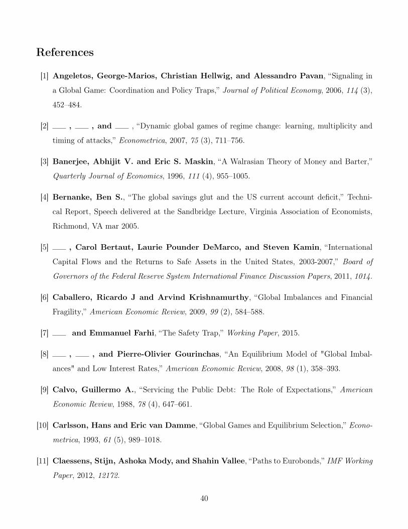
References
[1] Angeletos, George-Marios, Christian Hellwig, and Alessandro Pavan, “Signaling in
a Global Game: Coordination and Policy Traps,” Journal of Political Economy, 2006, 114 (3),
452–484.
[2] , , and , “Dynamic global games of regime change: learning, multiplicity and
timing of attacks,” Econometrica, 2007, 75 (3), 711–756.
[3] Banerjee, Abhijit V. and Eric S. Maskin, “A Walrasian Theory of Money and Barter,”
Quarterly Journal of Economics, 1996, 111 (4), 955–1005.
[4] Bernanke, Ben S., “The global savings glut and the US current account deficit,” Techni-
cal Report, Speech delivered at the Sandbridge Lecture, Virginia Association of Economists,
Richmond, VA mar 2005.
[5] , Carol Bertaut, Laurie Pounder DeMarco, and Steven Kamin, “International
Capital Flows and the Returns to Safe Assets in the United States, 2003-2007,” Board of
Governors of the Federal Reserve System International Finance Discussion Papers, 2011, 1014.
[6] Caballero, Ricardo J and Arvind Krishnamurthy, “Global Imbalances and Financial
Fragility,” American Economic Review, 2009, 99 (2), 584–588.
[7] and Emmanuel Farhi, “The Safety Trap,” Working Paper, 2015.
[8] , , and Pierre-Olivier Gourinchas, “An Equilibrium Model of "Global Imbal-
ances" and Low Interest Rates,” American Economic Review, 2008, 98 (1), 358–393.
[9] Calvo, Guillermo A., “Servicing the Public Debt: The Role of Expectations,” American
Economic Review, 1988, 78 (4), 647–661.
[10] Carlsson, Hans and Eric van Damme, “Global Games and Equilibrium Selection,” Econo-
metrica, 1993, 61 (5), 989–1018.
[11] Claessens, Stijn, Ashoka Mody, and Shahin Vallee, “Paths to Eurobonds,” IMF Working
Paper, 2012, 12172.
40

[12] Cole, Harold L and T J Kehoe, “Self-fulfilling debt crises,” Review of Economic Studies,
2000, 67, 91–116.
[13] Diamond, D W, “Debt Maturity and Liquidity Risk,” Quarterly Journal of Economics, aug
1991, 106 (3), 709–737.
[14] Diamond, Peter A., “National Debt in a Neoclassical Growth Model,” American Economic
Review, 1965, 55 (5), 1126–1150.
[15] Doepke, Matthias and Martin Schneider, “Money as a Unit of Account,” Working Paper,
2013.
[16] Eichengreen, Barry, “The Euro as a Reserve Currency,” Journal of Japanese and Interna-
tional Economies, 1998, 12 (4), 483–506.
[17] , “The rise and fall of the dollar (or when did the dollar replace sterling as the leading
reserve currency?),” NBER Working Papers, 2005, 11336.
[18] , Exorbitant Privilege: the rise and fall of the Dollar and the future of the international
monetary system, Oxford University Press, 2011.
[19] Frankel, Jeffrey, “On the dollar,” in “The New Palgrave Dictionary of Money and Finance,”
London: MacMillan Press, 1992.
[20] Freeman, Scott and Guido Tabellini, “The Optimality of Nominal Contracts,” Economic
Theory, 1998, 11 (3), 545–562.
[21] Goldstein, Itay and Ady Pauzner, “Demand-Deposit Contracts and the Probability of
Bank Runs,” Journal of Finance, jun 2005, 60 (3), 1293–1327.
[22] Gourinchas, Pierre-Oliver, Helene Rey, and Nicolas Govillot, “Exorbitant Privilege
and Exorbitant Duty,” Working Paper, 2010.
[23] Greenwood, Robin and Dimitri Vayanos, “Bond supply and excess bond returns,” Review
of Financial Studies, 2014, 27 (3), 663–713.
41

[24] Hassan, Tarek, “Country size, currency unions, and international asset returns,” Journal of
Finance, 2013, 68 (6), 2269–2308.
[25] He, Zhiguo and Konstantin Milbradt, “Endogenous liquidity and defaultable bonds,”
Econometrica, 2014, 82 (4), 1443–1508.
[26] and , “Dynamic debt maturity,” Working Paper, 2015.
[27] and Wei Xiong, “Dynamic debt runs,” Review of Financial Studies, 2012, 25, 1799–
1843.
[28] and , “Rollover Risk and Credit Risk,” Journal of Finance, 2012, 67 (2), 391–429.
[29] , Arvind Krishnamurthy, and Konstantin Milbradt, “What makes US government
bonds safe assets?,” American Economic Review Papers & Proceedings, 2015.
[30] Holmstrom, Bengt and Jean Tirole, “Private and Public Supply of Liquidity,” Journal of
Political Economy, feb 1998, 106 (1), 1–40.
[31] Kiyotaki, Nobuhiro and Randall Wright, “On Money as a Medium of Exchange,” Journal
of Political Economy, 1989, 97 (4), 927–954.
[32] Krishnamurthy, Arvind and Annette Vissing-Jorgensen, “The Aggregate Demand for
Treasury Debt,” Journal of Political Economy, 2012, 120 (2), 233–267.
[33] and , “The Impact of Treasury Supply on Financial Sector Lending and Stability,”
Working Paper, 2015.
[34] Krugman, Paul R., “The international role of the dollar: theory and prospect,” in “Exchange
rate theory and practice,” National Bureau of Economic Research, Inc., 1984, chapter NBER
Chapt.
[35] Lagos, Ricardo, “Asset prices and liquidity in an exchange economy,” Working Paper, 2005.
[36] Maggiori, Matteo, “Financial Intermediation, International Risk Sharing, and Reserve Cur-
rencies,” Working Paper, 2013.
42

[37] Morris, Stephen and Hyun S Shin, “Unique Equilibrium in a Model of Self-Fulfilling
Currency Attacks,” American Economic Review, jun 1998, 88 (3), 587–597.
[38] and , “Global Games: Theory and Applications,” in Mathias Dewatripont, Lars P
Hansen, and S. Turnovsky, eds., Advances in Economics and Econometrics, Cambridge Uni-
versity Press, 2003.
[39] and , “Illiquidity component of credit risk,” Working Paper, 2010.
[40] Rochet, Jean-Charles and Xavier Vives, “Coordination failure and the lender of last
resort: was Bagehot right after all?,” Journal of the European Economic Association, dec 2004,
2 (6), 1116–1147.
[41] Samuelson, Paul A., “An Exact Consumption-Loan Model of Interest with or without the
Social Contrivance of Money,” Journal of Political Economy, 1958, 66 (6), 467–482.
[42] Vayanos, Dimitri and Pierre-Olivier Weill, “A Search-Based Theory of the On-the-Run
Phenomenon,” Journal of Finance, 2008, 53 (3), 1361–1398.
A Main Appendix
A.1 Equilibrium with non-monotone strategies and zero recoveryWe now construct an equilibrium with non-monotone strategies and joint safety on the endogenously determinedinterval [δL, δH ]. Given this equilibrium, we will compute the minimum value of z = z for which this equilibriumexists. The possibility of joint safety means that our equilibrium construction using threshold strategies is no longerpossible. In a region where both countries are known to be safe (recall we consider the limit where σ → 0), investorsmust be indifferent between the two countries, thus equalizing bond returns. Outside the joint safety interval, i.e.,δ̃ ∈ [−δ̄, δL) ∪ (δH , δ̄], we are back to the case where the signal is so strong that only one country is safe.
We conjecture the following non-monotone strategy whereby investment in country 1 and in country 2 alternateson discrete intervals of length kσ and (2− k)σ, with k ∈ (0, 2). The investor j’s strategy given his private signal δjis φ (δj) ∈ {0, 1}:
φ (δj) =
0, δj < δL
1, δj ∈ [δL, δL + kσ] ∪ [δL + 2σ, δL + (2 + k)σ] ∪ [δL + 4σ, δL + (4 + k)σ] ∪ ...0, δj ∈ [δL + kσ, δL + 2σ] ∪ [δL + (2 + k)σ, δL + 4σ] ∪ [δL + (4 + k)σ, δL + 6σ] ∪ ...1, δj > δH
(A.1)
As we will show shortly, the non-monotone oscillation occurs only when both countries are safe, where the equilibriumrequires proportional investment in each safe country to equalize returns across two safe bonds. Clearly, k determinesthe fraction of agents in investing in country 1 when oscillation occurs, to which we turn next.
43
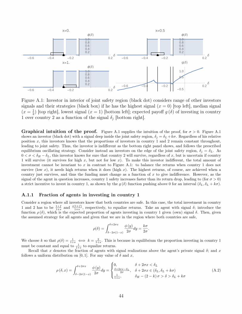
-0.6 -0.4 -0.2 0.2δ
0.20.40.60.81.0
ϕ(δ)x=0.
-0.6 -0.4 -0.2 0.2δ
0.20.40.60.81.0
ϕ(δ)x=0.5
-0.6 -0.4 -0.2 0.2δ
0.20.40.60.81.0
ϕ(δ)x=1.
-0.6 -0.4 -0.2 0.2δ
-0.5
0.5
1.0
g(δ)
Figure A.1: Investor in interior of joint safety region (black dot) considers range of other investorssignals and their strategies (black box) if he has the highest signal (x = 0) [top left], median signal(x = 1
2) [top right], lowest signal (x = 1) [bottom left]; expected payoff g (δ) of investing in country
1 over country 2 as a function of the signal δj [bottom right].
Graphical intuition of the proof. Figure A.1 supplies the intuition of the proof, for σ > 0. Figure A.1shows an investor (black dot) with a signal deep inside the joint safety region, δj = δL+kσ. Regardless of his relativeposition x, this investors knows that the proportions of investors in country 1 and 2 remain constant throughout,leading to joint safety. Thus, the investor is indifferent as the bottom right panel shows, and follows the prescribedequilibrium oscillating strategy. Consider instead an investors on the edge of the joint safety region, δj = δL. As0 < σ < δH − δL, this investor knows for sure that country 2 will survive, regardless of x, but is uncertain if country1 will survive (it survives for high x, but not for low x). To make this investor indifferent, the total amount ofinvestment cannot be invariant to x in contrast to Figure A.1: to balance the returns when country 1 does notsurvive (low x), it needs high returns when it does (high x). The highest returns, of course, are achieved when acountry just survives, and thus the funding must change as a function of x to give indifference. However, as thesignal of the agent in question increases, country 1 safety increases faster than its return drop, leading to (for σ > 0)a strict incentive to invest in country 1, as shown by the g (δ) function pushing above 0 for an interval (δL, δL + kσ).
A.1.1 Fraction of agents in investing in country 1Consider a region where all investors know that both countries are safe. In this case, the total investment in country1 and 2 has to be 1+f
1+s and s(1+f)1+s , respectively, to equalize returns. Take an agent with signal δ; introduce the
function ρ (δ), which is the expected proportion of agents investing in country 1 given (own) signal δ. Then, giventhe assumed strategy for all agents and given that we are in the region where both countries are safe,
ρ(δ) =
∫ δ+2σx
δ−2σ(1−x)
φ (y)
2σdy =
kσ
2σ.
We choose k so that ρ(δ) = 11+s ⇐⇒ k = 2
1+s . This is because in equilibrium the proportion investing in country 1
must be constant and equal to 11+s to equalize returns.
Recall that x denotes the fraction of agents with signal realizations above the agent’s private signal δ; and xfollows a uniform distribution on [0, 1]. For any value of δ and x,
ρ (δ, x) =
∫ δ+2σx
δ−2σ(1−x)
φ (y)
2σdy =
0, δ + 2σx < δLδ+2σx−δL
2σ , δ + 2σx ∈ (δL, δL + kσ)1
1+s , δH − (2− k)σ > δ > δL + kσ
(A.2)
44

When we evaluate δ at the marginal agent with signal δ = δL, we have
ρ (δL, x) =
0, x = 0
x, x ∈(
0, 11+s
)1
1+s , x > 11+s
(A.3)
where we observe that ρ (δL, x) is less than or equal to 11+s .
A.1.2 Lower boundary δL
Let Vφ (δ) be the expected payoff of strategy φ ∈ {0, 1} when given signal δ. In the completely safe region discussedabove (for δ exceeding δL sufficiently), investors were indifferent between both strategies. This is not the case foragent with signals around the threshold signal δL: as the agent knows investors with signal below are always investingin country 2, country 1 is a perceived default risk. We now calculate the return of investing in either country, fromthe perspective of the boundary agent δL.
For the boundary agent δL, the return from investing only in country 2 (i.e. φ = 0) is given by
Π2 (δL) =
∫ 1
0
s
(1 + f) (1− ρ(δL, x))dx (A.4)
where we integrate over all x as country 2 is safe regardless of x. We will show consistency of this assumption withthe derived equilibrium later. Thus, plugging in, we have
Π2 (δL) =s
1 + f
[∫ 11+s
0
1
1− xdx+
∫ 1
11+s
1s
1+s
dx
]=
s
1 + f
[ln
1 + s
s+ 1
]<
1 + s
1 + f. (A.5)
where we used s ln 1+ss < 1. Here, we see that payoff to investing in country 2 is lower than the expected payoff that
would have realized if both countries were safe. This reflects the strategic substitution effect: because more people(in expectation) invest in the safe country 2, the return in country 2 is lower.
Now we turn to country 1. Since country 1 has default risk, we need to calculate the threshold x = xmin sothat country 1 becomes safe if there are x > xmin measure of agents receiving better signals. To derive xmin, wefirst solve for ρmin1 (δ), which is the minimum proportion of agents investing in country 1 that are needed to makecountry 1 safe given fundamental δ. We have
θ1 (δ) + (1 + f) ρmin1 (δ) = 1 ⇐⇒ ρmin1 (δ) =1− θ1 (δ)
1 + f
Define xmin as the solution to ρ (δL, x) = ρmin1 (δL). Given equation (A.3), we have that,
xmin =1− θ1 (δL)
1 + f. (A.6)
The expected return of investing in country 1 given one’s own signal δL and the conjectured strategies φ (·) of everyoneelse is given by,
Π1 (δL) =
∫ 1
xmin
1
(1 + f) ρ(δL, x)dx =
1
1 + f
[∫ 11+s
xmin
1
xdx+
∫ 1
11+s
1
1/ (1 + s)dx
]
=1
1 + f
[ln
1
1 + s− lnxmin + s
]. (A.7)
The boundary agent δL must be indifferent between investing in either country, i.e., Π2 (δL) = Π1 (δL). Plugging
45

in (A.4) and (A.7), we have
s
1 + f
[ln
1 + s
s+ 1
]=
1
1 + f
[ln
1
1 + s− lnxmin + s
]⇐⇒ xmin =
ss
(1 + s)1+s . (A.8)
We combine our two equations for xmin, (A.6) and (A.8), and use 1− θ1 (δL) = (1− θ) exp (−δL), to obtain:
ss
(1 + s)1+s =
(1− θ) exp (−δL)
1 + f.
Recall z = ln 1+f1−θ ; we have
δL (z) = −z + (1 + s) ln (1 + s)− s ln s (A.9)
A.1.3 Upper boundary δH
The derivation is symmetric to the above. We have
ρ (δ, x) =
∫ δ+2σx
δ−2σ(1−x)
φ (y)
2σdy =
1
1+s , δ − 2σ (1− x) < δH − (2− k)σδ+2σx−δH
2σ δ − 2σ (1− x) ∈ (δH − (2− k)σ, δH)
1, δ − 2σ (1− x) > δH
(A.10)
so that
ρ (δH , x) =
1
1+s , x < 11+s
x, x ∈(
11+s , 1
)1, x = 1
(A.11)
which yields
Π1 (δH) =
∫ 1
0
1(1 + f̂
)ρ(δH , x)dy
dx =1
1 + f[ln (1 + s) + 1] <
1 + s
1 + f,
where we integrated over all x as country 1 is always safe in the vicinity of δH .The default condition for country 2 is
sθ2 (δH) + (1 + f) [1− ρmax2 (δH)] = s ⇐⇒ 1− ρmax2 (δH) = s1− θ2 (δH)
1 + f
where ρmax2 (δ) is the maximum amount of agents investing in country 1 so that country 2 does not default. Assume,but later verify, that at δH we have 1 − ρmax2 (δH) < s
1+s , that is, country 2 would survive even if less than s1+s of
investors invest in country 2. Define xmax (δH) as the solution to ρ (δH , xmax) = ρmax2 (δH); (A.11) implies that
1− xmax (δH) = s1− θ2 (δH)
1 + f. (A.12)
As a result, the return to country 2 is,
Π2 (δH) =
∫ xmax(δH)
0
s
(1 + f) (1− ρ(δH , x))dydx =
s
1 + f̂
[∫ 11+s
0
1
1− 11+s
dx+
∫ xmax(δH)
11+s
1
1− xdx
]
=s
1 + f
[1
s+ ln
s
1 + s− ln (1− xmax (δH))
]Indifference at the boundary agent δH requires Π1 (δH) = Π2 (δH), which yields 1−xmax (δH) = s
(1+s)1+ss
. Combining
46

this result with (A.12) and 1− θ2 (δH) = (1− θ) exp (δH), we solve,
δH (z) = z − 1 + s
sln (1 + s) (A.13)
A.1.4 Verifying the equilibriumWe now verify the interior agents δ ∈ (δL, δH) have the appropriate incentives to play the conjectured strategy, andthat our assumptions of country 1 (2) is always safe at δH (δL) are correct. As an investor with signal δ = δL isindifferent, it is easy to show that agents with δ < δL find it optimal to invest in country 2. Consider an investor withsignal δ = δL+kσ (i.e. let us consider the investors depicted by the black dot in Figure A.1). Regardless of his relativeposition (as measured by x) in the signal distribution, this agent knows that a proportion 1
1+s of investors invest incountry 1, thus making it safe for sure. Further, he knows that a proportion s
1+s of investors invest in country 2,also making it safe. Therefore, this agent knows that (i) both countries are completely safe and that (ii) investmentflows give arbitrage free prices. He is thus indifferent, and so is every investor with δL + kσ < δ < δH − (2− k)σ.
Next, we consider an investor with δ ∈ (δL, δL + kσ). We know that country 2 will always survive, and thus wehave
Π2 (δ) =
∫ 1
0
s
(1 + f)∫ δ+2σx
δ−2σ(1−x)1−φ(y)
2σ dydx.
Note that for any x with x ≥ − δ−δL−kσ2σ we are in the oscillating region; for x below we are in the increasing part.
Let ε ≡ δ−δL2σ ∈
(0, 1
1+s
)so that so that δ = δL + 2σε. Thus, we have
1− ρ (δ, x) =
∫ δ+2σx
δ−2σ(1−x)
1− φ (y)
2σdy =
1− ε− x, x ∈(
0, 11+s − ε
),
s1+s , x ∈
(1
1+s − ε, 1).
(A.14)
Then, we have
Π2 (δ) =s
1 + f
[∫ 11+s−ε
0
1
1− ε− xdx+
∫ 1
11+s−ε
1s
1+s
dx
]= Π2 (δL) +
s(ln (1− ε) + 1+s
s ε)
1 + f
For investment in country 1, we know that, since δ > δL, we have ρmin1 (δ) < ρmin1 (δL). First, note that
ρ (δ, x) =
∫ δ+2σx
δ−2σ(1−x)
φ (y)
2σdy =
ε+ x, x ∈(
0, 11+s − ε
)1
1+s , x ∈(
11+s − ε, 1
)Let xmin (δ) be the measure of investors with higher signals than δ so that country 1 is safe. Since ρmin1 (δ) = 1−θ1(δ)
1+f ,xmin (δ) is the lowest x ∈ [0, 1] such that
ρ (δ, x) = ε+ x ≥ ρmin1 (δ) .
Thus, we have
xmin (δ) = xmin (δL + 2σε) = max
{1− θ1 (δL + 2σε)
1 + f− ε, 0
}. (A.15)
The expected investment return from country 1 is
Π1 (δ) =
∫x:ρ(δ,x)≥ρmin1 (δ)
1
(1 + f)∫ δ+2σx
δ−2σ(1−x)φ(y)2σ dy
dx
= Π1 (δL) +1
1 + f{lnxmin (δL)− ln [ε+ xmin (δL + 2σε)] + (1 + s) ε}
47

Thus, to show that Π1 (δL + 2σε) ≥ Π2 (δL + 2σε), we need to show that the following inequality holds for ε ∈(0, 1
1+s
):
gL (ε) ≡ (1 + f) (Π1 −Π2) = lnxmin (δL)− ln [ε+ xmin (δL + 2σε)]− s ln (1− ε) ≥ 0. (A.16)
First, by using lnxmin (δL) = s ln s−(1 + s) ln (1 + s) and xmin(δL + 2σ 1
1+s
)= 0, we know the above inequality
holds with equality at both end points ε = 0 and ε = 11+s , i.e., gL (0) = gL
(1
1+s
)= 0. Second, it is easy to show that
there exists a unique ε∗ such that 1−θ1(δL+2σε∗)1+f = ε∗, at which point (A.15) binds at zero. We further note that at
ε = 0 we have 1−θ1(δL)1+f > 0. Thus, in (A.15) we have ε∗ > 0 and for ε ∈ (0, ε∗) we have xmin (δ) = 1−θ1(δL+2σε)
1+f −ε > 0,
and for ε ∈[ε∗, 1
1+s
]we have xmin (δ) = 0. Plugging in and taking derivative with respect to ε, we have
∂
∂εln [ε+ xmin (δL + 2σε)] =
−2σθ′1(δL+2σε)1−θ1(δL+2σε) , ε ∈ (0, ε∗)
1ε , ε ∈
[ε∗, 1
1+s
]Then, for (A.16), we have gL (ε) first rises and then drops:
g′L (ε) =
2σθ′1(δL+2σε)1−θ1(δL+2σε) + s
1−ε > 0 , ε ∈ (0, ε∗) ,
− 1ε + s
1−ε = (1+s)ε−11−ε < 0 , ε ∈
[ε∗, 1
1+s
].
Combined with gL (0) = gL
(1
1+s
)= 0 we know that gL (ε) > 0, ∀ε ∈
(0, 1
1+s
), i.e., Thus, on ε ∈
(0, 1
1+s
)the
investors strictly want to invest in country 1.We now consider the investors with δ ∈ (δH − (2− k)σ, δH). We know that country 1 will always survive, and
thus we have
Π1 (δ) =
∫ 1
0
1
(1 + f)∫ δ+2σx
δ−2σ(1−x)φ(y)2σ dy
dx.
Let ε ≡ δH−δ2σ ∈
(0, s
1+s
)so that so that δ = δH − 2σε. Thus, we have
ρ (δ, x) =
∫ δ+2σx
δ−2σ(1−x)
φ (y)
2σdy =
1
1+s , x ∈(
0, 11+s + ε
),
x− ε, x ∈(
11+s + ε, 1
).
(A.17)
Plugging in, we have
Π1 (δ) =1
1 + f
[∫ 11+s+ε
0
11
1+s
dx+
∫ 1
11+s+ε
1
x− εdx
]=
1
1 + f[1 + (1 + s) ε+ ln (1− ε) + ln (1 + s)] .
For investment in country 2, we know that, since δ < δH , we have 1−ρmax2 (δ) < 1−ρmax2 (δL) ⇐⇒ ρmax2 (δL) <ρmax2 (δ). First, note that
1− ρ (δ, x) =
∫ δ+2σx
δ−2σ(1−x)
1− φ (y)
2σdy =
s
1+s , x ∈(
0, 11+s + ε
),
1 + ε− x, x ∈(
11+s + ε, 1
).
Let xmax (δ) be the measure of investors with higher signals than δ so that country 2 is safe. Since 1 − ρmax2 (δ) =
s 1−θ2(δ)1+f , xmax (δ) is the highest x ∈ [0, 1] such that
1− ρ (δ, x) = 1 + ε− x ≤ 1− ρmax2 (δ) .
48

Thus, we have
xmax (δ) = xmax (δH − 2σε) = min
{1 + ε− s1− θ2 (δH − 2σε)
1 + f, 1
}. (A.18)
The expected investment return from country 2 is
Π2 (δ) =
∫x:ρ(δ,x)≤ρmax2 (δ)
s
(1 + f)∫ δ+2σx
δ−2σ(1−x)1−φ(y)
2σ dydx
=s
1 + f
[1 + s
s
(1
1 + s+ ε
)− ln [1 + ε− xmax (δ)] + ln
(s
1 + s
)]Differencing, we have
gH (ε) = (1 + f) [Π1 (ε)−Π2 (ε)] = ln (1− ε)− s ln s+ (1 + s) ln (1 + s) + s ln [1 + ε− xmax (δ)]
with similar properties to gL (ε).Finally, we need to pick σ appropriately so that there exists some natural number N > 1 so that 2Nσ = δH−δL.
For this particular choice of σ = σ̂, the limiting case of zero signal noise can be achieved when we take the sequenceof σn = σ̂/n for n = 1, 2, .....
A.1.5 Equilibrium propertiesFirst, with joint safety, the probability of survival for country 1 (or the probability of its bonds being the safe asset)is no longer one minus the probability of survival of country 2. Using δ̃ ∼ U
(−δ, δ
), the probability of country 1
survival is
Pr (country 1 safe) =δ − δL
2δ=δ + z − (1 + s) ln (1 + s) + s ln s
2δ, (A.19)
and the probability of country 2 survival is
Pr (country 2 safe) =δH + δ
2δ=δ + z − 1+s
s ln (1 + s)
2δ.
As a result, the bonds issued by country 1 are more likely to be the safe assets than that issued by country 2 if thefollowing condition holds:
s ln s− (1 + s) ln (1 + s) +1 + s
sln (1 + s) = s ln s+
(1
s− s)
ln (1 + s) > 0. (A.20)
This condition always holds: Define F (s) ≡ s2 ln s+(1− s2
)ln (1 + s), then F (s) > 0 holds for s ∈ (0, 1). It is clear
that F (0) = 0 while F (1) = 0. Simple algebra shows that
F ′ (s) = 2s ln s− 2s ln (1 + s) + 1,1
2F ′′ (s) = ln s− ln (1 + s) + 1− s
1 + s= ln
(s
1 + s
)+ 1− s
1 + s.
Let y = s1+s <∈ (0, 1); then because it is easy to show ln y + 1 − y < 0 (due to concavity of ln y), we know that
F ′′ (s) < 0. As a result, F (s) is concave but F (0) = F (1) = 0. This immediately implies that F (s) > 0, which isour desired result. The condition is the same if we focus on sole survivals only instead of sole and joint survival, i.e.,the bonds of country j are the only safe asset, the condition is exactly the same.
Country 1 has the highest likelihood of survival when s→ 0, which immediately follow from − (1 + s) ln (1 + s)+s ln s is decreasing in s.
Obviously, the above equilibrium construction requires that δL (z) < δH (z). Since δL (z) in (A.9) is decreasingin z while δH (z) in (A.13) is increasing in z, this condition δL (z) < δH (z) holds if z > z so that δL (z) = δH (z)
49

which gives z:
−z + (1 + s) ln (1 + s)− s ln s = z − 1 + s
sln (1 + s)⇒ z =
1
2
[(2 + s+
1
s
)ln (1 + s)− s ln s
]
A.2 Extension for a negative β assetSuppose that θ, which proxies for the aggregate fundamental for both countries, is subject to shocks. For convenience,suppose that θ̃ is drawn from the following uniform distribution θ̃ ∼ U
[θ, θ], and recall z
(θ̃)
= ln 1+f
1−θ̃ . Also, supposethat
li = lθ̃, i ∈ {1, 2}
where l > 0 is a positive constant, so that recovery is increasing in the fundamental shock. Using (15), we calculatethe threshold δ∗ (θ) as a function of the realization of θ̃ = θ, to be
δ∗ (θ) =[(1− lθ) s− (1− lθ)] z (θ)− (s+ lθ) ln (s+ lθ) + (1 + slθ) ln (1 + lθs) + lθ ln (lθ)− slθ ln (lθ)
(1− lθ) + s (1− lθ)
Note that ddθ δ∗ (θ) < 0; that is, a higher θ, by reducing rollover risk, makes country 1 safer.
In this exercise we consider a distribution so that the relative fundamental δ is almost surely, δ > δ∗ (E [θ]). Thisimplies that ex-ante country 1 bonds are more likely to be safe. Also, define θ̂ (δ) so that δ∗
(θ̂)
= δ holds; this is the
critical value of fundamental θ = θ̂ so that country 1’s bonds lose safety. We choose δ so that θ̂ > θ, which impliesthat with strictly positive probability, country 1 defaults given a sufficiently low fundamental.
We are interested in the β of the bond price of each country with respect to the θ shock, i.e.,
βi (δ) =Cov
(pi
(θ̃; δ), θ̃)
V ar(θ̃) =
E[pi
(θ̃; δ)· θ̃]− E
[θ̃]E[pi
(θ̃; δ)]
V ar(θ̃) , (A.21)
From equation (17), we know that
p1 (θ; δ) =
{(1+f)lθs+lθ if θ<θ̂ (δ) so country 1 defaults;1+f1+lθs if θ ≥ θ̂ (δ) so country 1 survives;
and
p2 (θ; δ) =
{1+fs+lθ if θ<θ̂ (δ) so country 2 survives;(1+f)lθ1+lθs if θ ≥ θ̂ (δ) so country 2 defaults.
Given these pricing functions, it is straightforward to evaluate βs in (A.21). We vary country 1’s relative strength δand plot the βs for both bonds as a function of δ in Figure 3. We only plot the β for country 1’s bonds, becauseβ2 = −β1/s in our model.11
A.3 Equilibrium with monotone strategies and joint bondsIn this appendix, we proof that δ∗ (α) is unique, δ∗ (α) ≤ 0, exists on [0, α∗] and has δ∗ (α∗) = 0.
First, assume s = 1. Then, conjecture that δ∗ (α) = 0 throughout by a simple symmetry argument. From (25),with θdef (δ∗ (α)) = θ, we then have
α∗ =1 + s
1 + f(1− θ) = e−z (1 + s) (A.22)
Next, assume s < 1 and ez > (1 + s) so that δ∗ (0) < 0. Then, let us conjecture δ∗ (α) ≤ 0 for α ∈ (0, α∗).
11This is because cash-in-the-market-pricing implies that p1 + sp2 = 1 + f .
50

Setting Π1 (δ∗) = Π2 (δ∗) from (20) after substituting in for f̂ from (23), δ∗ (α) is implicitly defined via
0 = h (δ∗, α) = ln
[ez
1− αe−δ∗ − α
1+sez
]− s ln
[ez
s
1− αeδ∗ − α
1+sez
](A.23)
Then, consider δ̃ = δ∗ (α)+. At this point, country 1 just survives, even though the funding gap (scaled by size)of country 2 is the best among all defaulting countries. Then, for the monotone cutoff strategy to be consistent, weneed the default condition
α ≤ 1 + s
1 + f[1− θ2 (δ∗)] =
1 + s
1 + f(1− θ) eδ
∗= e−z (1 + s) eδ
∗
Suppose that the constraint is binding, which defines a loosest δ∗ (α) by
δ̂∗ (α) = z + ln
(α
1 + s
)⇐⇒ eδ̂
∗(α) =α
1 + sez (A.24)
Assume that α < α∗ = 1+s1+f (1− θ). Plugging in δ̂∗ (α), we see that
h(δ̂∗ (α) , α
)= ln
[ez
1− αe−z 1+s
α −α
1+sez
]− s ln
[ez
s
1− αez α
1+s −α
1+sez
]< 0 (A.25)
as the second term explodes, i.e. ln [·] = ∞. Thus, it must be that 0 > δ∗ (α) > δ̂∗ (α)—the first part by ourassumption that δ∗ < 0 and the second by the construction. However, we note that δ̂∗ (α∗) = 0 so that δ∗ (α∗) = 0.This is possible as (δ, α) = (0, α∗) is a root of h – both sides are exploding at this point. The restriction above alsoimplies that 0 < δ∗α (α∗) < δ̂∗α (α∗) = 1
α∗ so that δ∗ (α) has a bounded and positive derivative at α∗.We next show that for a fixed α ∈ [0, α∗], there exists unique δ∗ (α) that solves h (δ∗, α). Fix α. Then, consider
h (δ∗, α) as a function of δ∗. Differentiating w.r.t. δ∗, we have
∂h (δ∗, α)
∂δ∗=
e−δ∗(eδ∗ − α
1+sez)
+ seδ∗(e−δ
∗ − α1+se
z)
(e−δ∗ − α
1+sez)(
eδ∗ − α1+se
z)
Then, given that we have α < α∗ and δ̂∗ (α) < δ∗ < 0 by assumption, we have(e−δ
∗− α
1 + sez)>
(e−δ
∗− α∗
1 + sez)
= e−δ∗− 1 > 0
by assumption on the sign of δ∗. Next, we have(eδ∗− α
1 + sez)>
(eδ̂∗(α) − α
1 + sez)
=α
1 + sez − α
1 + sez = 0
by the assumption on δ∗ ∈(δ̂∗ (α) , 0
). Thus, we have ∂h(δ∗,α)
∂δ∗ > 0. Finally, we know that h(δ̂∗ (α) , α
)< 0 <
h (0, α), so that a unique δ∗ (α) ∈(δ̂∗ (α) , 0
)exists.
What remains to be shown is that δ∗ (α) does not cross 0 before α∗. Suppose it does. Then, there exists anα̂ > 0 but α̂ 6= α∗ such that δ∗ (α̂) = 0. Then, we have
h (0, α̂) = ln
[ez
1− α̂1− α̂
1+sez
]− s ln
[ez
s
1− α̂1− α̂
1+sez
]= (1− s) ln
[ez
1− α̂1− α̂
1+sez
]+ s ln s
51

Setting this equal to 0, we have
ln
[1− α̂
1− α̂1+se
z
]=−s ln s
1 + s− z ⇐⇒ 1− e[
−s ln s1+s −z][
1− 11+se
[−s ln s1+s ]
] = α̂
Simplifying, we have
α̂ =(1 + s)
(1− s
−s1+s e−z
)1 + s− s
−s1+s
Then, notice that α̂ > α∗ ⇐⇒(1+s)
(1−s
−s1+s e−z
)1+s−s
−s1+s
> e−z (1 + s), which simplifies to 1 > α∗. Thus, the function
δ∗ (α) does not cross 0 before α∗.
A.4 Equilibrium with non-monotone strategies and joint bondsLet us conjecture a non-monotone oscillating strategy as in A.1.
A.4.1 Lower boundary δL.The definitions of ρ (δ, x) and ρ (δL, x) are as in Appendix A.1, and most of the result simply have f̂ instead of f : ascountry 2 is safe to an agent with δ = δL, we have Π2 (δL) = s
1+f̂
[ln 1+s
s + 1]< 1+s
1+f̂.
The common bonds change the safety condition for country 1 to
θ1 (δ) + αpc +(
1 + f̂)ρmin1 (δ) = 1 ⇐⇒ ρmin1 (δ) =
1− θ1 (δ)− αpc1 + f̂
Define xmin (δL) as the solution to ρ (δL, x) = ρmin1 (δL). Given equation (A.3), we have that,
xmin (δL) =1− θ1 (δL)− αpc
1 + f̂(A.26)
Again, the expected return of investing in country 1 is given by Π1 (δL) = 11+f̂
[ln 1
1+s − lnxmin (δL) + s]. Indifference
requires that Π2 (δL) = Π1 (δL), which implies that
xmin (δL) = exp [s ln s− (1 + s) ln (1 + s)] (A.27)
We combine the expressions for xmin (δL), (A.26) and (A.27), to solve for δL:
δL = − ln
{1
1− θ
[(1 + f̂
) ss
(1 + s)(1+s)
+ αpc
]}. (A.28)
A.4.2 Upper boundary δH.The derivation of ρ (δ, x) and ρ (δH , x) follow Appendix A.1, , and most of the result simply have f̂ instead of f . Wehave Π1 (δH) = ln(1+s)+1
1+f̂as country 1 is considered safe at δj = δH .
The default condition for country 2 is
sθ2 (δ) + sαpc +(
1 + f̂)
[1− ρmax2 (δ)] = s ⇐⇒ [1− ρmax2 (δ)] = s1− θ2 (δ)− αpc
1 + f̂
where ρmax2 (δ) is the maximum amount of people investing in country 1 so that country 2 does not default. Definexmax (δH) as the solution to ρ (δH , xmax) = ρmax2 (δH). Given equation (A.11), we have that,
52

1− xmax (δH) = s1− θ2 (δH)− αpc
1 + f̂(A.29)
Then the return to investing in country 2 is again given by Π2 (δH) = s1+f̂
[1s + ln s
1+s − ln (1− xmax (δH))].
Indifference requires Π1 (δH) = Π2 (δH), which implies that
1− xmax (δH) =s
(1 + s)1+ss
(A.30)
We combine the expressions for xmax (δH), (A.29) and (A.30), to solve for δH :
δH = ln
{1
1− θ
[1 + f̂
(1 + s)1+ss
+ αpc
]}(A.31)
The remainder of the proof, i.e., the verification argument, is exactly the same as in Appendix A.1 and henceomitted here.
A.4.3 Cutoff αHL < α∗.First, the assumption ez > (1 + s) ⇐⇒ (1 + f) > (1− θ) (1 + s) guarantees that there is some realizations of δ̃that would allow joint safety. Consider the total funding requirement,
total(δ̃)
= (1− θ1) + (1− θ2) s = (1− θ)(e−δ̃ + s · eδ̃
)(A.32)
This is minimized at δ̃ = − 12 ln s ≥ 0 for a total funding requirement of total
(− 1
2 ln s)
= (1− θ) 2√s. Next, note
that 1 + s > 2√s so that ez > (1 + s) > 2
√s.
Recall that α∗ = e−z (1 + s). Then, assume that z > ln (1 + s) so that α∗ ∈ (0, 1). Then, we have
δH (α∗)− δL (α∗) = ln
{ez
1 + s
[(1
1 + s
) 1s
(1− α∗) + α∗
]}+ ln
{ez
1 + s
[(s
1 + s
)s(1− α∗) + α∗
]}
= ln
[(1
1 + s
) 1s(
1
α∗− 1
)+ 1
]+ ln
[(s
1 + s
)s(1
α∗− 1
)+ 1
]> 0
where we used(
11+s
) 1s
< 1 and(
s1+s
)s< 1 and 1
α∗ > 1 in the last line. Thus, at α∗ the oscillating equilibriumalready exists. It is easy to show that the the joint safety region [δL (α) , δH (α)] is expanding uniformly in α, andthus that αHL < α∗.
Finally, define αHL as the solution to
0 = δH (αHL)− δL (αHL)
= 2 [z − ln (1 + s)] + ln
[(1
1 + s
) 1s
(1− αHL) + αHL
]+ ln
[(s
1 + s
)s(1− αHL) + αHL
]Rearranging, we have[(
1
1 + s
) 1s
(1− αHL) + αHL
] [(s
1 + s
)s(1− αHL) + αHL
]− e−2z (1 + s)
2= 0
which is a quadratic equation in αHL. We note that e−2z (1 + s)2< 1 ⇐⇒ 2 [ln (1 + s)− z] < 0, so that αHL = 1
makes the LHS positive. We also know that the LHS is increasing in αHL for αHL > 0. Thus, there exists at mostone positive root αHL ∈ (0, 1) under the assumption z > ln (1 + s), and if not, both roots are negative. Solving for
53

the larger root αHL, and after some algebra, we can show that δ∗ (αHL) = δH (αHL) = δL (αHL).
54

B Online Appendix
B.1 Additive Fundamental StructureWe have considered the specification of 1 − θi = (1− θ) exp
((−1)
iδ̃)for country i’s fundamental. We now show
that results are qualitatively similar with the alternative additive specification
θ1 = θ + δ̃, and θ2 = θ − δ̃.
As x = Pr(δ̃ + εj > δ∗
)= δ̃+σ−δ∗
2σ ⇒ δ̃ = δ∗ + (2x− 1)σ, we know that
θ1 = θ + δ̃ = θ + δ∗ + (2x− 1)σ
θ2 = θ − δ̃ = θ − δ∗ − (2x− 1)σ
Given x, the large country 1 survives if and only if
p1 − 1 + θ1 = (1 + f)x− 1 + θ + δ∗ + (2x− 1)σ ≥ 0⇔ x ≥ 1− θ − δ∗ + σ
1 + f + 2σ
which implies the expected return from investing in country 1 is
Π1 =
∫ 1
1−θ−δ∗+σ1+f+2σ
1
(1 + f)xdx =
1
1 + fln
1 + f + 2σ
1− θ − δ∗ + σ.
For country 2, the bond is paid back if
(1 + f)x′ − s+ sθ2 = (1 + f)x′ − s+ s [θ − δ∗ − (2x− 1)σ] ≥ 0
⇔ x′ ≥ s (1− θ + δ∗ − σ)
1 + f + 2sσ
which implies an expected return of
Π2 =
∫ 1
s(1−θ+δ∗−σ)1+f+2sσ
s
(1 + f)x′dx′ =
s
1 + fln
1 + f + 2sσ
s (1− θ + δ∗ + σ)
As a result, the equilibrium threshold δ∗ is pinned by by the indifference condition
ln1 + f + 2σ
1− θ − δ∗ + σ= s ln
1 + f + 2sσ
s (1− θ + δ∗ + σ).
Letting σ → 0 we obtain
ln1 + f
1− θ − δ∗= s ln
1 + f
s (1− θ + δ∗). (B.1)
We no longer have close-form solution for δ∗ in (B.1), as δ∗ shows up in both sides. However, the solution is uniquebecause LHS (RHS) is increasing (decreasing) in δ∗. Finally, to ensure δ∗ < 0 so that the larger country 1 is relativelysafer, we require the same sufficient condition of z = ln 1+f
1−θ > 1 in this alternative specification.
B.2 Uniqueness of the threshold equilibrium within monotone strategiesFirst, let us define a few primitives. Let δj be a generic signal, and δ be the true state of the world. Further, let xdenote the amount of pessimism of the investors, so that x = 1 is the most pessimistic agent (amongst all agents outthere) and x = 0 is the least pessimistic agent. We then have δ (δj , x) = δj + 2σ
(x− 1
2
). For most of the proofs,
we assume wlog that we the investor believes his signal to be the true signal, and thus all the action comes formmovements in his relative position. As σ → 0, fundamental uncertainty (that is movements in δ as a function of x)
Online Appendix B-1

will vanish, whereas strategic uncertainty (relative ranking of investors as represented by x) remains.Next, let us define φ (δj) as the proportion of funds an investor with signal δj invests in country 1. Then
define
ρ (δj , x) =1
2σ
∫ δj+2σx
δj−2σ(1−x)φ (y) dy
as the aggregate proportion of investors in country 1 an investor with signal δj and level of pessimism xexpects given the conjecture strategies φ (·). Note that there is translation invariance
ρ (δj , x) = ρ(δj + ε, x− ε
2σ
),∀x ∈
( ε
2σ, 1)
Finally, define the (scaled by 1 + f) expected difference in expected returns as
∆ (δj) =
∫ 1
0
1{ρ(δ,x)≥ρmin(δ)}1
ρ (δ, x)dx−
∫ 1
0
1{ρ(δ,x)≤ρmax(δ)}s
1− ρ (δ, x)dx
Then, for any given conjectured difference function ∆ (y), we must have
φ (y) =
1, ∆ (y) > 0
∈ [0, 1] , ∆ (y) = 0
0, ∆ (y) < 0
A monotone strategy is defined by φ′ (y) ≥ 0 for all y ∈[−δ, δ
], which implies that ρδ (δ, x) ≥ 0 as well as
ρx (δ, x) ≥ 0, i.e., ρ (δ, x) is monotone. This implies that we can write
∆ (δj) =
∫ 1
0
1{ρ(δj ,x)≥ρmin(δ(δj ,x))}1
ρ (δ, x)dx−
∫ 1
0
1{ρ(δj ,x)≤ρmax(δ(δj ,x))}s
1− ρ (δ, x)dx
≈∫ 1
0
1{ρ(δj ,x)≥ρmin(δj)}1
ρ (δ, x)dx−
∫ 1
0
1{ρ(δj ,x)≤ρmax(δj)}s
1− ρ (δ, x)dx
=
∫ 1
xmin(δj)
1
ρ (δj , x)dx−
∫ xmax(δj)
0
s
1− ρ (δj , x)dx
Country 1 survives if ρ (δj , x) is larger than ρmin (δ (δj , x)). As the agent becomes more pessimistic relative to theother agents, i.e., x increases, the actual relative fundamental increases, and thus the threshold decreases:
∂xρmin (δ (δj , x)) = ∂xe−ze−δ(δj ,x) = −e−ze−δ(δj ,x)2σ < 0
∂δjρmin (δ (δj , x)) = −e−ze−δ(δj ,x) < 0
Thus, if ρ (δ, x) is monotone, there exists a unique threshold xmin (δ) above which country 1 is safe. Further,by the implicit function theorem, we have
x′min (δ) = −ρδ (δ, x)− ∂δρmin
(δ̃ (δ, x)
)ρx (δ, x)− ∂xρmin
(δ̃ (δ, x)
)= −
φ(δ+2σx)−φ(δ−2σ(1−x))2σ + e−ze−δ̃(δ,x)
φ (δ + 2σx)− φ (δ − 2σ (1− x)) + e−ze−δ̃(δ,x)2σ
= − 1
2σ
Online Appendix B-2

so that the pessimism threshold falls that makes country 1 safe. Similarly, we have
x′max (δ) = −ρδ (δ, x)− ∂δρmax
(δ̃ (δ, x)
)∂x (δ, x)− ∂xρmax
(δ̃ (δ, x)
)= −
φ(δ+2σx)−φ(δ−2σ(1−x))2σ + se−zeδ̃(δ,x)
φ (δ + 2σx)− φ (δ − 2σ (1− x)) + se−zeδ̃(δ,x)2σ
= − 1
2σ
We can thus approximate
xmax (δ + ε) +ε
2σ≈ xmax (δ) + x′max (δ) ε+
ε
2σ= xmax (δ) and xmin (δ + ε) +
ε
2σ≈ xmin (δ)
Finally, suppose a δ exists for which the investor expects joint safety, i.e., both countries to be safe for sure.Then, we must have φ (δ) = 1
1+s by the no arbitrage condition. A threshold equilibrium is defined by a single-crossing condition on ∆ = Π1−Π2 and a non-flat part at 0, where ∆ (δ) > 0 implies φ = 1 and ∆ (δ) < 0 impliesφ = 0. Consider any other equilibrium. By dominance regions, we know that for high δ, φ = 1 will eventually beoptimal, and for very low δ, φ = 0 will eventually be optimal.
Thus, any other equilibrium is either characterized by (1) a flat part ∆ (δ) = 0, (2) multiple crossings ∆ (δ) = 0or (3) a combination of the two. In our oscillating strategy, (3) is the case, with a flat part in the middle.
B.2.1 Monotonicity and uniqueness of threshold equilibriumA monotone strategy φ (δ) requires ∆ (δ) to change signs only once. Thus, ∆ (δ) either crosses zero at a single point,or approaches it from below, stays flat on an interval [δL, δH ], and then rises above zero. Thus, at any point δ s.t.∆ (δ) = 0 we must have ∆′ (δ) ≥ 0. As we want to show that a threshold equilibrium is the only equilibrium possible,we now rule out any flat parts of ∆ at zero.
To this end, suppose an interval [δL, δH ] exists on which ∆ (δ) = 0.
Interior xmin, xmax. Suppose now that xmin (δ) , xmax (δ) ∈ (0, 1). This means that both countries are atrisk of default, so there is no possibility of joint safety across all possible x ∈ [0, 1] (it might exists for some x ifxmin (δ) < xmax (δ)). Take ε ∈ (0, δH − δL). Then, we write
Π1 (δ + ε) =
∫ 1
xmin(δ+ε)
1
ρ (δ + ε, x)dx
=
∫ 1+ ε2σ
xmin(δ+ε)+ε2σ
1
ρ(δ + ε, x− ε
2σ
)dx=
∫ 1
xmin(δ+ε)+ε2σ
1
ρ(δ + ε, x− ε
2σ
)dx+
∫ 1+ ε2σ
1
1
ρ(δ + ε, x− ε
2σ
)dx≈
∫ 1
xmin(δ)
1
ρ (δ, x)dx+
∫ 1
1− ε2σ
1
ρ (δ + ε, x)dx
= Π1 (δ) +
∫ 1
1− ε2σ
1
ρ (δ + ε, x)dx︸ ︷︷ ︸
new pessimists
Online Appendix B-3

Similarly, we have
Π2 (δ + ε) =
∫ xmax(δ+ε)
0
s
1− ρ (δ + ε, x)dx
=
∫ xmax(δ+ε)+ε2σ
ε2σ
s
1− ρ(δ + ε, x− ε
2σ
)dx≈
∫ xmax(δ)
ε2σ
s
1− ρ (δ, x)dx+
∫ ε2σ
0
s
1− ρ (δ, x)dx−
∫ ε2σ
0
s
1− ρ (δ, x)dx
=
∫ xmax(δ)
0
s
1− ρ (δ, x)dx−
∫ ε2σ
0
s
1− ρ (δ, x)dx
= Π2 (δ)−∫ ε
2σ
0
s
1− ρ (δ, x)dx︸ ︷︷ ︸
old optimists
so that
∆ (δL + ε) = Π1 (δL + ε)−Π2 (δL + ε)
= Π1 (δL) +
∫ 1
1− ε2σ
1
ρ (δL + ε, x)dx−
[Π2 (δL)−
∫ ε2σ
0
s
1− ρ (δL, x)dx
]
=
∫ 1
1− ε2σ
1
ρ (δL + ε, x)dx+
∫ ε2σ
0
s
1− ρ (δL, x)dx > 0
But this implies thatφ (δL + ε) = 1
By monotonicity then, δL is the only point at which ∆ (δ) = 0 and no flat parts can exist for xmin, xmax ∈ (0, 1).
Cornered xmin, xmax. Next, suppose that at least one of the countries is going to survive regardless of x becauseof the assumed strategies. Wlog, let us focus on δL. First, let us rule out that xmin (δL) = 0. Note that for anyε > 0, we have by the dominance boundaries ∆ (δL − ε) < 0 and ∆ (δH + ε) > 0, the highest and lowest point of theall flat parts. Further note that xmin (δL) = 0 implies that country 1 always survives in the eyes of an investor withsignal δL. By construction we have ρ (δ, 0) = 0— when the agent with signal δL is the most optimistic agent, hemust believe by the conjecture on ∆ (δ) that everyone below him investors fully into country 2. But then this agentcannot believe that country 1 is safe regardless of x, as by assumption no country can survive without a minimumamount of investment.
Thus, at δL we must have xmax (δL) = 1 and xmin (δH) = 0—country 2 always survives given the strategiesof the different agents. Then, we have the survival boundary of country 2 not changing, and thus again for ε ∈
Online Appendix B-4

(0, δH − δL) we have
Π2 (δ + ε) =
∫ 1
0
s
1− ρ (δ + ε, x)dx
=
∫ 1+ ε2σ
ε2σ
s
1− ρ(δ + ε, x− ε
2σ
)dx=
∫ 1
ε2σ
s
1− ρ (δ, x)dx+
∫ 1
1− ε2σ
s
1− ρ (δ + ε, x)dx
=
∫ 1
0
s
1− ρ (δ, x)dx+
∫ 1
1− ε2σ
s
1− ρ (δ + ε, x)dx−
∫ ε2σ
0
s
1− ρ (δ, x)dx
= Π2 (δ) +
∫ 1
1− ε2σ
s
1− ρ (δ + ε, x)dx︸ ︷︷ ︸
new pessimists
−∫ ε
2σ
0
s
1− ρ (δ, x)dx︸ ︷︷ ︸
old optimists
Then, we have
0 = ∆ (δ + ε) = Π1 (δ + ε)−Π2 (δ + ε)
= Π1 (δ) +
∫ 1
1− ε2σ
1
ρ (δ + ε, x)dx−
[Π2 (δ) +
∫ 1
1− ε2σ
s
1− ρ (δ + ε, x)dx−
∫ ε2σ
0
s
1− ρ (δ, x)dx
]
=
∫ 1
1− ε2σ
1
ρ (δ + ε, x)dx−
∫ 1
1− ε2σ
s
1− ρ (δ + ε, x)dx+
∫ ε2σ
0
s
1− ρ (δ, x)dx
=
∫ 1
1− ε2σ
[1
ρ (δ + ε, x)− s
1− ρ (δ + ε, x)
]dx︸ ︷︷ ︸
new pessimists
+
∫ ε2σ
0
s
1− ρ (δ, x)dx︸ ︷︷ ︸
old optimists
and there is now a possibility of a flat part. The intuition here is that we are balancing the returns that arise to thenew most pessimistic investor (i.e. for high x) against the previous expected returns of the most optimistic investors(i.e. low x).
Taking derivatives around ε = 0, we have
∆ (δ + ε) ≈ ∆ (δ) + ∆′ (δ) ε
=1
2σ
[1
ρ(δ + ε, 1− ε
2σ
) − s
1− ρ(δ + ε, 1− ε
2σ
)]ε=0
ε
+
[∫ 1
1− ε2σ
[−ρδ (δ + ε, x)
ρ (δ + ε, x)2 −
s (−ρδ (δ + ε, x))
[1− ρ (δ + ε, x)]2
]dx
]ε=0
ε
+1
2σ
[s
1− ρ(δ, ε2σ
)]ε=0
ε
=1
2σ
[1
ρ (δ, 1)− s
1− ρ (δ, 1)+
s
1− ρ (δ, 0)
]ε
When δ = δL we must have ρ (δL, 0) = 0 by definition of δL. Then, the derivative ∆′ (δL) = 0 if
ρ (δL, 1) =−1 +
√1 + 4s
2s>
1
1 + s
which implies that least on for some points on (δL, δL + 2σ) we have φ (δ) > 11+s .
By x′min (δ) ≤ 0 and x′max (δ) ≤ 0, as δ increases either we (i) move to a segment where xmin (δ) , xmax (δ) ∈ (0, 1),
Online Appendix B-5

an interior situation, or (ii) to a segment with xmin (δ) = 0, xmax (δ) = 1, a completely safe part.But we know from the previous section that (i) immediately has ∆′ (δ) > 0, a violation of the premise that we
are on a flat part for δ ∈ [δL, δH ]. Next, consider for (ii) any completely safe subset J ⊂ (δL, δH) and δ ∈ J . Then,we require ρ (δ, x) = 1
1+s ,∀x ∈ [0, 1] by no arbitrage, which implies φ (δ) = 11+s . But then we have a violation of
monotonicity as ρ (δL, 1) > 11+s . Thus, there cannot be any flat parts of ∆ (δ) at zero and the only equilibrium that
survives is of the threshold form. By the construction in the paper, this threshold equilibrium is unique.
Existence of threshold equilibrium. Consider our unique candidate equilibrium
δ∗ = −1− s1 + s
z − s ln s
1 + s
derived in the main text. Consider now δj < δ∗. Then, we have
∆ (δj ; δ∗) =
∫ρ(x)>ρmin(δ̃(x;δj))
1
(1 + f) ρ (x)dx− s
∫ρ(x)<ρmax(δ̃(x;δj))
1
(1 + f) (1− ρ (x))dx
We know that ∆ (δ∗; δ∗) = 0. But by our setup, we know that moving δj < δ∗ lowers both ρmin (δ) and ρmax (δ).Thus, we need to look at the difference between the parts we are adding (region in which country 1 survives) andparts we are subtracting (region in which country 2 survives):
∆δj (δj ; δ∗) = −ρ′min (δj)
1
(1 + f) ρmin (δj)+ sρ′max (δj)
1
(1 + f) (1− ρmax (δj))
=1
(1 + f)− s 1
(1 + f)=
1− s1 + f
> 0
where we used
ρ′min (δj) = −ρmin (δj) and ρ′max (δj) = − (1− ρmax (δj))
This is intuitive: as we increase δj , we are adding the most valuable states for country 1 (fixing ρ (x)) by evaluatingat points set on which it will just survive, i.e., close to ρmin (δj), and we are taking away the most valuable statesfor country 2 by evaluating at points set on which it will just default, i.e., close to ρmax (δj).
B.3 Equilibrium with non-monotone strategies and positive recoveryLet us say that s1 = 1, s2 = s and lisi to be the recovery given default of country i, so that it returns lisi
yiper unit
of dollar invested, where yi is total investment in country i. Then if country 1 survives, to equalize return, we need
l2s
y2=
1
y1, y1 + y2 = 1 + f ⇒ y1
y2=
1
l2s.
This gives prices equal to
p1 = y1 =(1 + f)
1 + l2s
p2 =y2s
=(1 + f) l21 + l2s
Similarly, if country 2 survives, then
s
y2=l1y1, y1 + y2 = 1 + f ⇒ y1
y2=l1s
Online Appendix B-6

which results in prices
p1 = y1 =(1 + f) l1l1 + s
p2 =y2s
=(1 + f)
l1 + s
Letz = ln
1 + f
1− θ> 0
and fiscal surplus is given by
θ1 = 1− (1− θ) e−δ = 1− (1 + f) e−ze−δ
sθ2 = s[1− (1− θ) eδ
]= s
[1− (1 + f) e−zeδ
]Define two constants k1 > 1 and k2 > 1 (which only occurs if s < l1) so that
k12− k1
=1
l2s⇐⇒ k1 =
2
1 + l2s> 1
k22− k2
=s
l1⇐⇒ k2 =
2s
s+ l1> 1
Then in the country-1-default region, k2σ measure of agents invest in country 2, i.e. play φ = 0, while (2− k2)σmeasure of agents play φ = 1. Similarly in the country-2-default region, , k1σ measure of agents play φ = 1 while(2− k1)σ measure of agents play φ = 0.
Conjecture the following equilibrium with cut off δ∗
φ (y) =
....
1, y ∈ [δ∗ − 2σ, δ∗ − k2σ]
0, y ∈ [δ∗ − k2σ, δ∗]1, y ∈ [δ∗, δ∗ + k1σ]
0, y ∈ [δ∗ + k1σ, δ∗ + 2σ]
1, y ∈ [δ∗ + 2σ, δ∗ + 2σ + k1σ]
....
In other words, two types of equilibria collide at δ∗. I conjecture that marginal investor at δ∗ is indifferent, whilethe agents between [δ∗ − k2σ, δ∗] strictly prefer φ = 0, and symmetrically the agents between [δ∗, δ∗ + k1σ] strictlyprefer φ = 1. Other agents in this economy are indifferent.
Let x denote the fraction of agents with signal realization above the agent’s private signal δj , so that given x,the true fundamental is
δ (x) = δj − (1− 2x)σ
Further, let ρ (δj , x) be the expected proportion agents investing in country 1 given x. Then, we have
ρ (δj , x) =
1− k2
2 , δ + 2σx < δ∗ + (2− k2)σ
x+ cst, elsek12 δ − 2σ (1− x) > δ∗ − (2− k1)σ
where cst is picked so that ρ (δj , x) is continuous in x. We note that the slope is generically x as we are replacing
Online Appendix B-7

φ = 0 with φ = 1 marginally. At δj = δ∗, we have
ρ (δ∗, x) =
1− k2
2 , x < 1− k22
x, elsek12 x > k1
2
and we need1− k2
2<k12
Note that if we assume that ρmin (δ) , 1− ρmax (δ) ∈[1− k2
2 ,k12
]we have a 1-to-1 function between x and ρ that
yields
xmin =1− θ1 (δ∗)
1 + f=
1− θ1 + f
e−δ∗⇐⇒ lnxmin = −z − δ∗
1− xmax = s1− θ2 (δ∗)
1 + f= s
1− θ1 + f
eδ∗⇐⇒ ln (1− xmax) = ln s− z + δ∗
Note here that we are ignoring fundamental uncertainty. Otherwise, we need to take account of the fact that in themind of the agent,
ρmin (δ (x)) = e−ze−δ(x) = e−ze−[δj−(1−2x)σ]
is the minimum investment in country 1 needed for it to survive conditional on x. For everything else below, weassume that ρmin (δ (x)) = ρmin (δj). Next, note that
x = Fraction of people with signal above agent
so that x = 1 is the most pessimistic agent, and x = 0 is the most optimistic. As ρ (δ, x) is increasing in x, we have
x < xmin ⇐⇒ Country 1 failsx > xmin ⇐⇒ Country 1 survivesx < xmax ⇐⇒ Country 2 survivesx > xmax ⇐⇒ Country 2 fails
Then, for the boundary agent, the expected return of investing in country 2 is given by
Π2 (δ∗) = Return2 (survival) +Return2 (default)
=
∫ xmax
0
s
(1 + f) (1− ρ (δ∗, x))dx+
∫ 1
xmax
l2s
(1 + f) (1− ρ (δ∗, x))dx
=
∫ 1− k22
0
s
(1 + f)(1−
(1− k2
2
))dx+
∫ xmax
1− k22
s
(1 + f) (1− x)
+
∫ k12
xmax
l2s
(1 + f) (1− x)dx+
∫ 1
k12
l2s
(1 + f)(1− k1
2
)dx=
(1− k2
2
)s
(1 + f) k22+
s
1 + f
[ln
(k22
)− ln (1− xmax)
]+
l2s
1 + f
[ln (1− xmax)− ln
(1− k1
2
)]+
(1− k1
2
)l2s
(1 + f)(1− k1
2
)=
s
(1 + f)
{(1− k2
2k22
)+
[ln
(k22
)− ln (1− xmax)
]+ l2 + l2
[ln (1− xmax)− ln
(1− k1
2
)]}
Online Appendix B-8

and the expected return of investing in country 1 is given by
Π1 (δ∗) =
∫ xmin
0
l1(1 + f) ρ (δ∗, x)
dx+
∫ 1
xmin
1
(1 + f) ρ (δ∗, x)dx
=
∫ 1− k22
0
l1
(1 + f)(1− k2
2
)dx+
∫ xmin
1− k22
l1(1 + f)x
dx
+
∫ k12
xmin
1
(1 + f)xdx+
∫ 1
k12
1
(1 + f) k12dx
=
(1− k2
2
)l1
(1 + f)(1− k2
2
) +l1
1 + f
[ln (xmin)− ln
(1− k2
2
)]+
1
1 + f
[ln
(k12
)− ln (xmin)
]+
(1− k1
2
)1
(1 + f) k12
=1
1 + f
{l1 + l1
[ln (xmin)− ln
(1− k2
2
)]+
[ln
(k12
)− ln (xmin)
]+
(1− k1
2k12
)}
Note that (1− k1
2k12
)=
(1k12
− 1
)= 1 + sl2 − 1 = sl2(
1− k22
k22
)=
(1k22
− 1
)=
s+ l1s− s
s=l1s
Setting these equal, we have
s
{l1s
+
[ln
(k22
)− ln (1− xmax)
]+ l2 + l2
[ln (1− xmax)− ln
(1− k1
2
)]}=
{l1 + l1
[ln (xmin)− ln
(1− k2
2
)]+
[ln
(k12
)− ln (xmin)
]+ sl2
}Plugging in for k1, k2 and
k12
=1
1 + l2sk22
=s
s+ l1
1− k12
=l2s
1 + l2s
1− k22
=l1
s+ l1ln (xmin) = −z − δ∗
ln (1− xmax) = −z + δ∗ + ln s
Online Appendix B-9

Setting these equal, we have
s
{[ln
(k22
)− ln (1− xmax)
]+ l2
[ln (1− xmax)− ln
(1− k1
2
)]}= l1
[ln (xmin)− ln
(1− k2
2
)]+
[ln
(k12
)− ln (xmin)
]⇐⇒ s
{− (1− l2) ln (1− xmax) +
[ln
(k22
)− l2 ln
(1− k1
2
)]}= − (1− l1) ln (xmin) +
[ln
(k12
)− l1 ln
(1− k2
2
)]⇐⇒ s
{(1− l2) (z − δ∗ − ln s) +
[ln
(s
s+ l1
)− l2 ln
(l2s
1 + l2s
)]}= (1− l1) (z + δ∗) +
[ln
(1
1 + l2s
)− l1 ln
(l1
s+ l1
)]Finally, solving for δ∗, we have
δ∗ =s{
(1− l2) (z − ln s) +[ln(
ss+l1
)− l2 ln
(l2s
1+l2s
)]}− (1− l1) z −
[ln(
11+l2s
)− l1 ln
(l1s+l1
)](1− l1) + s (1− l2)
=s {(1− l2) z − (1− l2) ln s+ ln s− ln (s+ l1)− l2 ln l2 − l2 ln s+ l2 ln (1 + l2s)}
(1− l1) + s (1− l2)
+− (1− l1) z + ln (1 + l2s) + l1 ln (l1)− l1 ln (s+ l1)
(1− l1) + s (1− l2)
so that finally
δ∗ =[(1− l2) s− (1− l1)] z − (s+ l1) ln (s+ l1) + (1 + sl2) ln (1 + l2s) + l1 ln l1 − sl2 ln l2
(1− l1) + s (1− l2)(B.2)
Plugging in l1 = l2 = 0, we have
δ∗ =− (1− s) z − s ln (s)
1 + s
just as we had before.We want to show that from the perspective of δ∗, for an x small enough so that ρ (δ∗, x) = 1− k2
2 , does country1 default? We know that ρmin (δ∗) = e−ze−δ
∗, so that
ρmin (δ∗) > 1− k22
⇐⇒ ln (ρmin (δ∗)) > ln
(1− k2
2
)⇐⇒ − (δ∗ + z) > ln
(l1
s+ l1
)which gives
− [2 (1− l2) sz − (s+ l1) ln (s+ l1) + (1 + sl2) ln (1 + l2s) + l1 ln l1 − sl2 ln l2]
> [(1− l1) + s (1− l2)] [ln l1 − ln (s+ l1)]
and ultimately yields
F ∗1 (l1, l2, s)] ≡ −2 (1− l2) sz − [1 + s (1− l2)] ln l1 + sl2 ln l2 + [1 + s (2− l2)] ln (s+ l1)− (1 + l2s) ln (1 + l2s)
Online Appendix B-10

and the default condition is given by F ∗1 (l1, l2, s) ≥ 0. Assume l1 = l2 = l. Then, we have
F ∗1 (l, l, s) = −2 (1− l) sz − [1− (1− 2l) s] ln l + [1 + s (2− l)] ln (s+ l)− (1 + ls) ln (1 + ls)
We can show that F ∗1 (l, l, s) is always positive for small enough recovery l as the term − [1− (1− 2l) s] ln l explodes,swamping any negative z effect.12
Next, we want to show that from the perspective of δ∗, for an x large enough so that ρ (δ∗, x) = k12 , does country
2 default? We know that 1− ρmax (δ∗) = se−zeδ∗, so that
1− ρmax (δ∗) > 1− k12
⇐⇒ ln (1− ρmax (δ∗)) > ln
(1− k1
2
)⇐⇒ ln s− z + δ∗ > ln
(l2s
1 + l2s
)so that
[(1− l1) + s (1− l2)] ln s− 2 (1− l1) z − (s+ l1) ln (s+ l1) + (1 + sl2) ln (1 + l2s) + l1 ln l1 − sl2 ln l2
> [(1− l1) + s (1− l2)] [ln l2 + ln s− ln (1 + l2s)]
Define
F ∗2 (l1, l2, s) ≡ −2 (1− l1) z − (s+ l1) ln (s+ l1) + (2− l1 + s) ln (1 + l2s) + l1 ln l1 − [s+ (1− l1)] ln l2
and the default condition is given by F ∗2 (l1, l2, s) ≥ 0. Assuming equal recovery l1 = l2 = l, we have
F ∗2 (l, l, s) = −2 (1− l) z − (s+ l) ln (s+ l) + (2− l + s) ln (1 + ls)− [s+ (1− 2l)] ln l
We can show that F ∗2 (l, l, s) is always positive for small enough recovery l as the term − [s+ (1− 2l)] ln l explodes,swamping any negative z effect.
Let us consider an interior agent, i.e., δ ∈ [δ∗ − k2σ, δ∗ + k1σ]. Let
δ (ε) = δ∗ + 2εσ
with ε ∈[−k22 ,
k12
]. Let us first consider investment in country 1. We have ρmin (δ) as the default boundary, and
actual investment is given by
ρ (δ, x) =
1− k2
2 , δ∗ + ε2σ + 2σx < δ∗ + (2− k2)σ
x+ cst, elsek12 δ∗ + ε2σ − 2σ (1− x) > δ∗ − (2− k1)σ
=
1− k2
2 , 2εσ + 2σx < (2− k2)σ
x+ cst, elsek12 2εσ − 2σ (1− x) > − (2− k1)σ
which gives
ρ (δ, x) =
1− k2
2 , ε+ x < 1− k22
x+ ε, elsek12 ε+ x > k1
2
12Taking derivatives w.r.t. l and s, we have
∂lF∗1 (l, l, s) = 2sz + s− (1 + s)
l+
1 + (2− l) ss+ l
+ 2s ln l − s ln (s+ l)− s ln (1 + ls)
∂sF∗1 (l, l, s) =
1 + (2− l) ss+ l
− l ln (1 + ls) + (2− l) ln (s+ l)− 2 (1− l) z − l − (1− 2l) ln l
Online Appendix B-11

Note that we have cst = ε by imposing continuity (which has to follow from ρ (δ, x) being an integral over strategiesφ).
Let xmin (δ) be the lowest x ∈ [0, 1] such that
ρ (δ, x) = ε+ x ≥ ρmin (δ)
and we therefore havexmin (δ) = max {ρmin (δ)− ε, 0}
Similarly, let xmax (δ) be the highest x ∈ [0, 1] such that
1− ρ (δ, x) = 1− ε− x ≥ 1− ρmax (δ)
and thus1− xmax (δ) = max {1− ρmax (δ) + ε, 0}
The expected return of investing in country 1 is then given by
Π1 (δ) =
∫x:ρ(δ,x)<ρmin(x)
l1(1 + f) ρ (δ, x)
dx+
∫x:ρ(δ,x)≥ρmin(x)
1
(1 + f) ρ (δ, x)dx
=
∫ xmin(δ)
0
l1(1 + f) ρ (δ, x)
dx+
∫ 1
xmin(δ)
1
(1 + f) ρ (δ, x)dx
=
∫ 1− k22 −ε
0
l1
(1 + f)(1− k2
2
)dx+
∫ xmin(δ)
1− k22 −ε
l1(1 + f) (x+ ε)
dx
+
∫ k12 −ε
xmin(δ)
1
(1 + f) (x+ ε)dx+
∫ 1
k12 −ε
1
(1 + f) k12dx
=l1
1 + f
[1− k2
2 − ε1− k2
2
+ ln (xmin (δ) + ε)− ln
(1− k2
2
)]
+1
1 + f
[ln
(k12
)− ln (xmin (δ) + ε) +
1− k12 + εk12
]
=l1
1 + f
[1− ε
1− k22
+ ln (xmin (δ) + ε)− ln
(1− k2
2
)]
+1
1 + f
[ln
(k12
)− ln (xmin (δ) + ε) +
1− k12
k12
+εk12
]
= Π1 (δ∗) +l1
1 + f
[− ε
1− k22
+ ln (xmin (δ) + ε)− lnxmin (δ∗)
]
+1
1 + f
[lnxmin (δ∗)− ln (xmin (δ) + ε) +
εk12
]
= Π1 (δ∗) +1
1 + f
{ε
(1k12
− l1
1− k22
)− (1− l1) [ln (xmin (δ) + ε)− lnxmin (δ∗)]
}
= Π1 (δ∗) +1
1 + f{ε [(1− l1)− s (1− l2)]− (1− l1) [ln (xmin (δ) + ε)− lnxmin (δ∗)]}
Online Appendix B-12

Similarly, investing in country 2 gives
Π2 (δ) =
∫ xmax(δ)
0
s
(1 + f) (1− ρ (δ, x))dx+
∫ 1
xmax(δ)
l2s
(1 + f) (1− ρ (δ, x))dx
=
∫ 1− k22 −ε
0
s
(1 + f)(1−
(1− k2
2
))dx+
∫ xmax(δ)
1− k22 −ε
s
(1 + f) (1− x− ε)
+
∫ k12 −ε
xmax(δ)
l2s
(1 + f) (1− x− ε)dx+
∫ 1
k12 −ε
l2s
(1 + f)(1− k1
2
)dx=
s
1 + f
[1− k2
2 − εk22
+ ln
(k22
)− ln (1− xmax (δ)− ε)
]
+sl2
1 + f
[ln (1− xmax (δ)− ε)− ln
(1− k1
2
)+
1− k12 + ε
1− k12
]
= Π2 (δ∗) +s
1 + f
{ε
(l2
1
1− k12
− 1k22
)+ (1− l2) [ln (1− xmax (δ∗))− ln (1− xmax (δ)− ε)]
}
= Π2 (δ∗) +s
1 + f
{ε
[(1− l1)− s (1− l2)
s
]+ (1− l2) [ln (1− xmax (δ∗))− ln (1− xmax (δ)− ε)]
}Let us define
g (ε) ≡ (1 + f) [Π1 (δ)−Π2 (δ)]
= ε [(1− l1)− s (1− l2)]− (1− l1) [ln (xmin (δ) + ε)− lnxmin (δ∗)]
−s{ε
[(1− l1)− s (1− l2)
s
]+ (1− l2) [ln (1− xmax (δ∗))− ln (1− xmax (δ)− ε)]
}= − (1− l1) [ln (xmin (δ∗ + 2σε) + ε)− lnxmin (δ∗)]
+s (1− l2) [ln (1− xmax (δ∗ + 2σε)− ε)− ln (1− xmax (δ∗))]
+ε
{[(1− l1)− s (1− l2)]− s
[(1− l1)− s (1− l2)
s
]}= − (1− l1) [ln (xmin (δ∗ + 2σε) + ε)− lnxmin (δ∗)]
+s (1− l2) [ln (1− xmax (δ∗ + 2σε)− ε)− ln (1− xmax (δ∗))]
Taking the derivative w.r.t. ε, we have many different cases. The issue is if xmin or xmax start binding first.Regardless, close to ε = 0 we have neither xmin or xmax cornered, so that
ln (xmin (δ∗ + 2σε) + ε) = ln (ρmin (δ (ε))) = −z − δ (ε) = −z − (δ∗ + 2σε)
ln (1− xmax (δ∗ + 2σε)− ε) = ln (1− ρmax (δ (ε))) = s ln s− z + δ (ε) = s ln s− z + (δ∗ + 2σε)
and thus for ε small we have
g′ (ε) = − (1− l1) (−) 2σ + s (1− l2) 2σ = 2σ [(1− l1) + s (1− l2)] > 0
and indeed we have the incentives of the agents aligned with the conjectured strategies, at least around δ∗.Next, we have to account for all the different cases – that is, we know that at some distance ε that xmin, xmax
start binding at 0, 1, respectively.Let εmin be the point at which xmin becomes cornered, that is
ρmin (δ) = ε ⇐⇒ e−ze−(δ∗+2σε) = ε ⇐⇒ 2σε+ ln ε = −z − δ∗
Note that ρmin (δ) > 0 so that there is no solution for ε < 0.
Online Appendix B-13

Similarly, let εmax be the point at which xmax becomes cornered, that is
1− ρmax (δ) = −ε ⇐⇒ se−zeδ∗+2σε = −ε ⇐⇒ 2σ (−ε) + ln (−ε) = ln s− z + δ∗
Note that 1− ρmax (δ) ≥ 0 so that there is no solution for ε > 0.
Positive ε. Consider positive ε. Thus, we only have to worry about xmin cornered. When xmin becomes cornered,then
∂
∂εln (xmin (δ∗ + 2σε) + ε) =
1
ε
Then, we have
g′ (ε) = − (1− l1)1
ε+ s (1− l2) 2σ
The derivative is increasing in ε, and is largest at ε = k12 at a value of
g′(k12
)= − (1− l1) (1 + l2s) + s (1− l2) 2σ
For small enough σ, this is always negative.
Negative ε. Consider negative ε. Thus, we only have to worry about xmax cornered. When xmax becomescornered, then
∂
∂εln (1− xmax (δ∗ + 2σε)− ε) = −1
ε
Then, we have
g′ (ε) = (1− l1) 2σ + s (1− l2)
(−1
ε
)The derivative is again increasing in ε, and is largest at ε = −k22 at a value of
g′(−k2
2
)= − (1− l2) (s+ l1) + (1− l1) 2σ
For small enough σ, this is always negative.For s = 1 and l1 = l2 = l, we have symmetric conditions.The last thing we need to do is to check that
g
(−k2
2
)= g (0) = g
(k12
)= 0
To this end, we can also proof that as σ → 0, indeed one country (which one depending on on which side of δ∗ therealization of δ falls) will always default. This is equivalent to the interior assumption for xmax, xmin we made. Forthis to hold, we need the following restrictions
1− k12≤ 1− ρmax (δ∗) ≤ k2
2(B.3)
1− k22
≤ ρmin (δ∗) ≤ k12
(B.4)
The first line says that as σ → 0, if δ < δ∗ then a proportion k22 of investors invests in country 2, and it survives.
However, if δ > δ∗, then only a proportion 1− k12 of investors invests in country 2, and it defaults. Similar arguments
hold for country 1, which is summarized by the second line.
Online Appendix B-14

This can be rewritten as
ln
(1− k1
2
)≤ ln (1− ρmax (δ∗)) ≤ ln
(k22
)ln
(1− k2
2
)≤ ln ρmin (δ∗) ≤ ln
(k12
)which gives
ln
(l2s
1 + l2s
)≤ ln s− z + δ∗ ≤ ln
(s
s+ l1
)ln
(l1
s+ l1
)≤ −z − δ∗ ≤ ln
(1
1 + l2s
)equivalent to
ln
(l2
1 + l2s
)+ z ≤ δ∗ ≤ ln
(1
s+ l1
)+ z
ln
(l1
s+ l1
)+ z ≤ −δ∗ ≤ ln
(1
1 + l2s
)+ z
equivalent to
ln (l2)− ln (1 + l2s) + z ≤ δ∗ ≤ − ln (s+ l1) + z
− ln
(1
1 + l2s
)− z ≤ δ∗ ≤ − ln
(l1
s+ l1
)− z
equivalent to
ln (l2)− ln (1 + l2s) + z ≤ δ∗ ≤ − ln (s+ l1) + z
ln (1 + l2s)− z ≤ δ∗ ≤ ln (s+ l1)− ln (l1)− z
so that finally
max [ln (l2)− ln (1 + l2s) + z, ln (1 + l2s)− z] ≤ δ∗ ≤ min [− ln (s+ l1) + z, ln (s+ l1)− ln (l1)− z] (B.5)
The first term is binding on the RHS for z > ln (1 + l2s) − 12 ln (l2), and the first term is binding on the left hand
side for z < ln (s+ l1)− 12 ln (l1).
Online Appendix B-15