Embed Size (px)
Citation preview
A Model Reference Adaptive Search Methodfor Stochastic Global Optimization
Jiaqiao HuDepartment of Electrical and Computer Engineering & Institute for Systems Research,
University of Maryland, College Park, MD 20742, [email protected]
Michael C. FuRobert H. Smith School of Business & Institute for Systems Research,
University of Maryland, College Park, MD 20742, [email protected]
Steven I. MarcusDepartment of Electrical and Computer Engineering & Institute for Systems Research,
University of Maryland, College Park, MD 20742, [email protected]
September, 2005
Abstract
We propose a new method called Stochastic Model Reference Adaptive Search (SMRAS)for finding a global optimal solution to a stochastic optimization problem in situations wherethe objective functions cannot be evaluated exactly, but can be estimated with some noise(or uncertainty), e.g., via simulation. SMRAS is a generalization of the recently proposedModel Reference Adaptive Search (MRAS) method for deterministic global optimization withappropriate adaptations required for stochastic domains. We prove that SMRAS convergesasymptotically to a global optimal solution with probability one for both stochastic continuousand discrete (combinatorial) problems. Numerical studies are also carried out to illustrate themethod.
Keywords: stochastic optimization, global optimization, combinatorial optimization.
1 Introduction
Stochastic optimization problems arise in a wide range of areas such as manufacturing, communi-cation networks, system design, and financial engineering. These problems are typically much moredifficult to solve than their deterministic counterparts, either because an explicit relation betweenthe objective function and the underlying decision variables is unavailable or because the cost of aprecise evaluation of the objective function is too prohibitive. Oftentimes, one has to use simulationor real-time observations to evaluate the objective function. In such situations, all the objectivefunction evaluations will contain some noise, so special techniques are generally used (as opposedto the deterministic optimization methods) in order to filter out the noisy components. There aresome obvious distinctions between the solution techniques for stochastic optimization when thedecision variable is continuous and when it is discrete. Although some techniques, in principle, canbe applied to both types of problems, they require some suitable modifications in order to switch
1

from one setting to another. The work of this paper presents a unified approach to handle bothtypes of problems.
A well-known class of methods for solving stochastic optimization problems with continuousdecision variables is stochastic approximation (SA). These methods mimic the classical gradient-based search method in deterministic optimization, and rely on the estimation of the gradient ofthe objective function with respect to the decision variables. Because they are gradient-based,these methods generally find local optimal solutions. In terms of the different gradient estimationtechniques employed, the SA algorithms can be generally divided into two categories: algorithmsthat are based on direct gradient estimation techniques, the best-known of which are perturbationanalysis (PA) and the likelihood ratio/score function (LR/SF) method, and algorithms that arebased on indirect gradient estimation techniques like finite difference and its variations. A detailedreview of various gradient estimation techniques can be found in Fu (2005).
When the underlying decision variables are discrete, one popular approach is to use randomsearch. This has given rise to many different stochastic discrete optimization algorithms, includingthe stochastic ruler method and its modification (Yan and Mukai 1992; Alrefaei and Andradottir2001), the random search methods of Andradottir (1995) and (1996), modified simulated annealing(Alrefaei and Andradottir 1999), and the nested partitions method of Shi and Olafsson (2000). Themain idea throughout is to construct a Markov chain over the solution space and show that theMarkov chain settles down on the set of (possibly local) optimal solutions.
From an algorithmic point of view, there is another class of randomized search techniques,which Zlochin et al. (2004) have termed the model-based search methods (note that Markov chaintechniques are sometimes used in analyzing these methods), that can also be applied to stochasticdiscrete optimization problems. In general, most of the algorithms that fall in this category areiterative methods involving the following two steps:
1. Generate candidate solutions (e.g., random samples) according to a specified probabilisticmodel.
2. Update the probabilistic model, on the basis of the data collected in the previous step, inorder to bias the future search toward the region containing high quality solutions.
Two well-established model-based methods are the Stochastic Ant Colony Optimization (S-ACO)(Gutjahr 2003) and the Cross-Entropy (CE) method (Rubinstein and Kroese 2004). The S-ACOmethod is the extension of the original Ant Colony Optimization (ACO) algorithm (Dorigo andGambardella 1997) to stochastic problems. The method uses Monte-Carlo sampling to estimatethe objective and is shown (under some regularity assumptions) to converge to the global optimalsolution for stochastic combinatorial problems with probability one. The CE method was motivatedby an adaptive algorithm for estimating probabilities of rare events. It was later realized that themethod can be modified to solve deterministic optimization problems (cf. e.g., Rubinstein 1999).More recently, Rubinstein (2001) shows that the method is also capable of handling stochasticnetwork combinatorial optimization problems, and in that context, establishes the probability oneconvergence of the algorithm.
2
In this paper, we propose a new model-based search method, called stochastic model referenceadaptive search (SMRAS), for solving both continuous and combinatorial stochastic optimizationproblems. SMRAS is a generalization of the recently proposed MRAS method for deterministicoptimization (Hu et al. 2005) with some appropriate modifications and extensions required for thestochastic setting. The idea behind the method, as in MRAS for deterministic optimization, is to usea pre-specified parameterized probability distribution to generate candidate solutions, and to use asequence of convergent reference distributions to facilitate and guide the updating of the parametersassociated with the parameterized distribution at each step of the iteration procedure. A majormodification from the original MRAS method is in the way the sequence of reference distributionsis constructed. In MRAS, reference distributions are idealized probabilistic models constructedbased on the exact performance of the candidate solutions. In the stochastic case, however, theobjective function cannot be evaluated deterministically, so the sample average approximationsof the (idealized) reference distributions are used in SMRAS to guide the parameter updating.We show that for a class of parameterized distributions, the so-called Natural Exponential Family(NEF), SMRAS converges with probability one to a global optimal solution for both stochasticcontinuous and discrete problems. To the best of our knowledge, SMRAS is the first model-basedsearch method for solving both continuous and discrete stochastic optimization problems withprovable convergence.
The rest of the paper is structured as follows. In Section 2, we give a detailed descriptionof the SMRAS method. In Section 3, we show the asympotic global convergence properties ofthe method. Supporting numerical studies on both continuous and combinatorial optimizationproblems are given in Section 4. Finally some future research topics are outlined in Section 5.
2 The Stochastic Model Reference Adaptive Search Method
We consider the following optimization problem:
x∗ ∈ arg maxx∈X
Eψ[H(x, ψ)], (1)
where the solution space X is a non-empty set in <n, H(·, ·) is a deterministic, real-valued function,and ψ is a random variable (possibly depending on x) representing the stochastic effects of thesystem. We let h(x) := Eψ[H(x, ψ)]. Note that in many cases, h(x) cannot be obtained easily,but the random variable H(x, ψ) can be observed, e.g., via simulation. Throughout this paper, weassume that (1) has a unique global optimal solution, i.e., ∃x∗ ∈ X such that h(x) < h(x∗) ∀x 6=x∗, x ∈ X .
2.1 General Framework
SMRAS works with a family of parameterized distributions f(·, θ), θ ∈ Θ on the solution space,where Θ is the parameter space. The basic algorithmic structure is very simple. The main body ofthe method consists of two steps: (1) Generate candidate solutions from the current sampling
3
distribution, say f(·, θk). (2) Compute a new parameter vector θk+1 according to a specifiedparameter updating rule by using the candidate solutions generated in the previous step in orderto concentrate the future search toward more promising regions.
In SMRAS, the parameter updating rule is determined by another sequence of distributionsgk(·), called the reference distributions. In particular, at each iteration k, we look at the projectionof gk(·) on the family of distributions f(·, θ) and compute the new parameter vector θk+1 thatminimizes the Kullback-Leibler (KL) distance
D(gk, f(·, θ)) := Egk
[ln
gk(X)f(X, θ)
]=
∫
Xln
gk(x)f(x, θ)
gk(x)ν(dx),
where ν is the Lebesgue/counting measure defined on X , X = (X1, . . . , Xn) is a random vectortaking values in X with distribution gk(·), and Egk
[·] is the expectation taken with respect tothe distribution gk(·). Intuitively speaking, f(·, θk+1) can be viewed as a compact representation(approximation) of the reference distribution and thus may share some similar properties withgk(·). Therefore, the feasibility and effectiveness of the method will, to a large extent, depend onthe choices of the reference distributions. One basic property the sequence gk(·) should haveis convergence. There could be many different ways to construct such a convergent sequence ofdistributions. When the performance measure is deterministic, Hu et al. (2005) have proposed thefollowing simple iterative method for constructing gk(·). Let g0(x) > 0, ∀x ∈ X be an initialprobability density/mass function (p.d.f./p.m.f.) on the solution space X . Then, at each iterationk ≥ 1, compute a new p.d.f./p.m.f. by tilting the old p.d.f./p.m.f. gk−1(x) with the performancefunction h(x) (for simplicity, here we assume that h(x) > 0, ∀x ∈ X ), i.e.,
gk(x) =h(x)gk−1(x)∫
X h(x)gk−1(x)ν(dx), ∀x ∈ X . (2)
It is possible to show that the sequence gk(·) constructed above will converge to a distributionthat concentrates only on the optimal solution, regardless of the initial g0(·) used. However, in thestochastic setting, since the performance function h(·) cannot be evaluated exactly, the iterationprocedure given by (2) is no longer applicable. Thus, in SMRAS, one key modification of theoriginal deterministic algorithm is to use approximations gk(·) of gk(·) as the sequence ofreference distributions, which are constructed based on the sample average approximation of theperformance function h(·). Although this extension is conceptually straightforward, the detailedtechnical development is very involved.
2.2 Algorithm Description
In SMRAS, there are two allocation rules. The first one, denoted by Nk, k = 0, 1 . . ., is calledthe sampling allocation rule, where each Nk determines the number of candidate solutions to begenerated from the current sampling distribution at the kth iteration. The second is the observa-tion allocation rule Mk, k = 0, 1, . . ., which allocates Mk simulation observations to each of thecandidate solutions generated at the kth iteration. We require both Nk and Mk to increase as the
4
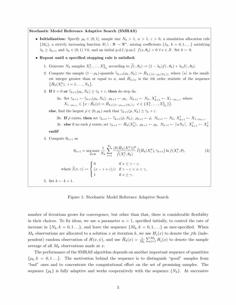
Stochastic Model Reference Adaptive Search (SMRAS)
• Initialization: Specify ρ0 ∈ (0, 1], sample size N0 > 1, α > 1, ε > 0, a simulation allocation ruleMk, a strictly increasing function S(·) : < → <+, mixing coefficients λk, k = 0, 1, . . . satisfyingλk ≥ λk+1 and λk ∈ (0, 1) ∀ k, and an initial p.d.f./p.m.f. f(x, θ0) > 0 ∀x ∈ X . Set k ← 0.
• Repeat until a specified stopping rule is satisfied:
1. Generate Nk samples Xk1 , . . . , Xk
Nkaccording to f(·, θk) := (1− λk)f(·, θk) + λkf(·, θ0).
2. Compute the sample (1 − ρk)-quantile γk+1(ρk, Nk) := Hk,(d(1−ρk)Nke), where dae is the small-est integer greater than or equal to a, and Hk,(i) is the ith order statistic of the sequenceHk(Xk
i ), i = 1, . . . , Nk
.
3. If k = 0 or γk+1(ρk, Nk) ≥ γk + ε, then do step 3a.
3a. Set γk+1 ← γk+1(ρk, Nk), ρk+1 ← ρk, Nk+1 ← Nk, X†k+1 ← X1−ρk+1 , where
X1−ρk+1 ∈x : Hk(x) = Hk,(d(1−ρk+1)Nke), x ∈ Xk
1 , . . . , XkNk.
else, find the largest ρ ∈ (0, ρk) such that γk+1(ρ, Nk) ≥ γk + ε.
3b. If ρ exists, then set γk+1 ← γk+1(ρ, Nk), ρk+1 ← ρ, Nk+1 ← Nk, X†k+1 ← X1−ρk+1 .
3c. else if no such ρ exists, set γk+1 ← Hk(X†k), ρk+1 ← ρk, Nk+1 ← dαNke, X†
k+1 ← X†k.
endif
4. Compute θk+1 as
θk+1 = arg maxθ∈Θ
1Nk
Nk∑
i=1
[S(Hk(Xki ))]k
f(Xki , θk)
I(Hk(Xk
i ), γk+1
)ln f(Xk
i , θ), (3)
where I(x, γ) :=
0 if x ≤ γ − ε,(x− γ + ε)/ε if γ − ε < x < γ,1 if x ≥ γ.
5. Set k ← k + 1.
Figure 1: Stochastic Model Reference Adaptive Search
number of iterations grows for convergence, but other than that, there is considerable flexibilityin their choices. To fix ideas, we use a parameter α > 1, specified initially, to control the rate ofincrease in Nk, k = 0, 1 . . ., and leave the sequence Mk, k = 0, 1, . . . as user-specified. WhenMk observations are allocated to a solution x at iteration k, we use Hj(x) to denote the jth (inde-pendent) random observation of H(x, ψ), and use Hk(x) = 1
Mk
∑Mkj=1 Hj(x) to denote the sample
average of all Mk observations made at x.The performance of the SMRAS algorithm depends on another important sequence of quantities
ρk, k = 0, 1 . . .. The motivation behind the sequence is to distinguish “good” samples from“bad” ones and to concentrate the computational effort on the set of promising samples. Thesequence ρk is fully adaptive and works cooperatively with the sequence Nk. At successive
5
iterations of the algorithm, a sequence of thresholds γk, k = 1, 2, . . . is generated according to thesequence of sample (1− ρk)-quantiles, and only those samples that have performances better thanthese thresholds will be used in parameter updating. Thus, each ρk determines the approximateproportion of Nk samples that will be used to update the probabilistic model at iteration k.
During the initialization step of SMRAS, a small positive number ε and a strictly increasingfunction S(·) : < → <+ are specified. The role of the parameter ε, as we will see later, is to filterout the observation noise. The function S(·) is used to account for cases where the sample averageapproximations Hk(x) are negative for some x.
At each iteration k, random samples are drawn from the density/mass function f(·, θk), whichis a mixture of the initial density f(·, θ0) and the density calculated from the previous iterationf(·, θk). The initial density f(·, θ0) can be chosen according to some prior knowledge of the problemstructure; however, if nothing is known about where the good solutions are, this density shouldbe chosen in such a way that each region in the solution space will have an (approximately) equalprobability of being sampled. Intuitively, mixing in the initial density enables the algorithm toexplore the entire solution space and thus maintain a global perspective during the search process.
At step 2, the sample (1−ρk)-quantile γk+1 with respect to f(·, θk) is calculated by first orderingthe sample performances Hk(Xk
i ), i = 1, . . . , Nk from smallest to largest, Hk,(1) ≤ Hk,(2) ≤ · · · ≤Hk,(Nk), and then taking the d(1 − ρk)Nketh order statistic. We use the function γk+1(ρk, Nk) toemphasize the dependencies of γk+1 on both ρk and Nk, so that different sample quantile valuescan be distinguished by their arguments.
Step 3 of the algorithm is used to construct a sequence of thresholds γk, k = 1, 2, . . . fromthe sequence of sample quantiles γk, and to determine the appropriate values of the ρk+1 andNk+1 to be used in subsequent iterations. This is carried out by checking whether the conditionγk+1(ρk, Nk) ≥ γk + ε is satisfied. If the inequality holds, then both the current ρk value andthe new sample size Nk are satisfactory, and γk+1(ρk, Nk) is used as the current threshold value.Otherwise, we fix the sample size Nk and try to find a smaller ρ < ρk such that the above inequalitycan be satisfied with the new sample (1− ρ)-quantile. If such a ρ does exist, then the current samplesize Nk is still deemed acceptable, and the new threshold value is updated by the sample (1− ρ)-quantile. On the other hand, if no such ρ can be found, then the sample size Nk is increased by afactor α, and the new threshold γk+1 is calculated by using an additional variable X†
k to rememberthe particular sample that achieves the previous threshold value γk, and then simply allocatingMk observations to X†
k. If more than one sample achieves the threshold value, ties are brokenarbitrarily.
It is important to note that in step 4, the setx : Hk(x) > γk+1− ε, x ∈ Xk
1 , . . . , XkNk could
be empty, since it could happen that all the random samples generated at the current iteration aremuch worse than those generated at the previous iteration. If this is the case, then by the definitionof I(·, ·, ), the right hand side of equation (3) will be equal to zero, so any θ ∈ Θ is a maximizer;we define θk+1 := θk in this case. Note that a “soft” threshold function I(·, ·), as opposed to theindicator function, is used in parameter updating (cf. equations (3)). The reason for doing so, aswill be seen later, is to smooth out the noisy observations.
6
We now show that there is a sequence of reference models gk(·) implicit in SMRAS, and theparameter θk+1 computed at step 4 indeed minimizes the KL-divergence D(gk+1, f(·, θ)).
Lemma 2.1 The parameter θk+1 computed at the kth iteration of SMRAS minimizes the KL-divergence D (gk+1, f(·, θ)), where
gk+1(x) :=
[[S(Hk(x))]k/f(x,θk)
]I(Hk(x),γk+1)
∑Nki=1
[[S(Hk(Xk
i ))]k/f(Xki ,θk)
]I(Hk(Xk
i ),γk+1)if
x : Hk(x) > γk+1 − ε, x ∈ Xk
1 , . . . , XkNk 6= ∅,
gk(x) otherwise,(4)
∀ k = 0, 1, . . ., where γk+1 :=
γk+1(ρk, Nk) if step 3a is visited,γk+1(ρ, Nk) if step 3b is visited,Hk(X†
k) if step 3c is visited.
Proof: We only need to consider the case wherex : Hk(x) > γk+1−ε, x ∈ Xk
1 , . . . , XkNk 6= ∅,
since if this is not the case, then we can always backtrack and find a gk(·) with non-empty support.For brevity, we define Sk(Hk(x)) := [S(Hk(x))]k
f(x,θk). Note that at the kth iteration, the K-L diver-
gence between gk+1(·) and f(·, θ) can be written as
D (gk+1, f(·, θ)) = Egk+1[ln gk+1(X)]−Egk+1
[ln f(X, θ)]
= Egk+1[ln gk+1(X)]−
1Nk
∑Nki=1 Sk(Hk(Xk
i ))I(Hk(Xk
i ), γk+1
)ln f(Xk
i , θ)1
Nk
∑Nki=1 Sk(Hk(Xk
i ))I(Hk(Xk
i ), γk+1
) ,
where X is a random variable with distribution gk+1(·), and Egk+1[·] is the expectation taken with
respect to gk+1(·). Thus the proof is completed by observing that minimizing D (gk+1, f(·, θ)) isequivalent to maximizing the quantity 1
Nk
∑Nki=1 Sk(Hk(Xk
i ))I(Hk(Xk
i ), γk+1
)ln f(Xk
i , θ).
Remark 1: When the solution space is finite, it is often beneficial to make efficient use of the pastsampling information. This can be achieved by maintaining a list of all sampled candidate solutions(along with the number of observations made at each of these solutions), and then check if a newlygenerated solution is in that list. If a new solution at iteration k has already been sampled and, sayMl, observations have been made, then we only need to take Mk−Ml additional observations fromthat point. This procedure is often effective when the solution space is relatively small. However,when the solution space is large, the storage and checking cost could be quite expensive. In SMRAS,we propose an alternative approach: at each iteration k of the method, instead of remembering allpast samples, we only keep track of those samples that fall in the region
x : Hk(x) > γk+1 − ε
.
As we will see, the sampling process will become more and more concentrated on these regions;thus the probability of getting repeated samples typically increases.
Remark 2: We have not provided a stopping rule for SMRAS; the discussion of this issue isdeferred to the end of the next section.
7
3 Convergence Analysis
Global convergence and computational efficiency of SMRAS clearly depend on the choice of theparameterized family of distributions. Throughout this paper, we restrict our discussion to the nat-ural exponential family (NEF), which works well in practice, and for which convergence propertiescan be established.
Definition 3.1 A parameterized family of p.d.f ’s f(·, θ), θ ∈ Θ ⊆ <m on X is said to belong tothe natural exponential family (NEF) if there exist functions `(·) : <n → <, Γ(·) : <n → <m, andK(·) : <m → < such that
f(x, θ) = expθT Γ(x)−K(θ)
`(x), ∀ θ ∈ Θ, (5)
where K(θ) = ln∫x∈X exp
θT Γ(x)
`(x)ν(dx), and “T” denotes vector transposition. For the case
where f(·, θ) is a p.d.f., we assume that Γ(·) is a continuous mapping.
Many p.d.f.’s/p.m.f.’s can be put into the form of NEFs; some typical examples are Gaussian,Poisson, binomial, geometric, and certain multivariate forms of them.
We make the following assumptions about the noisy observations Hj(x) and the observationallocation rule Mk.Assumptions:
L1. For any given ε > 0, these exists a positive number n∗ such that for all n ≥ n∗,
supx∈X
P(∣∣∣ 1
n
n∑
j=1
Hj(x)− h(x)∣∣∣ ≥ ε
)≤ φ(n, ε),
where φ(·, ·) is strictly decreasing in its first argument and non-increasing in its second argu-ment. Moreover, φ (n, ε) → 0 as n →∞.
L2. For any ε > 0, there exist positive numbers m∗ and n∗ such that for all m ≥ m∗ and n ≥ n∗,
supx,y∈X
P(∣∣∣ 1
m
m∑
j=1
Hj(x)− 1n
n∑
j=1
Hj(y)− h(x) + h(y)∣∣∣ ≥ ε
)≤ φ (minm,n, ε) ,
where φ(·, ·) satisfies the conditions in L1.
L3. The observation allocation rule Mk, k = 0, 1, . . . satisfies Mk ≥ Mk−1 ∀ k = 1, 2, . . ., andMk → ∞ as k → ∞. Moreover, for any ε > 0, there exist δε ∈ (0, 1) and Kε > 0 such thatα2kφ(Mk−1, ε) ≤ (δε)k, ∀ k ≥ Kε, where φ(·, ·) is defined as in L1.
Remark 3: Assumption L1 is satisfied by many random sequences, e.g., the sequence of i.i.d.random variables with (asymptotically) uniformly bounded variance, or a class of random variables(not necessarily i.i.d.) that satisfy the large deviations principle; please refer to Hong and Nelson
8
(2005) for further details. Assumption L2 can be viewed as a simple extension of L1. Most randomsequences that satisfy L1 will also satisfy L2. For example, consider the particular case wherethe sequence Hj(x), j = 1, 2, . . . is i.i.d. with uniformly bounded variance σ2(x) and E(Hj(x)) =h(x), ∀ x ∈ X . Thus the variance of the random variable 1
m
∑mj=1 Hj(x)− 1
n
∑nj=1 Hj(y) is 1
mσ2(x)+1nσ2(y), which is also uniformly bounded on X . By Chebyshev’s inequality, we have for any x, y ∈ X
P(∣∣∣ 1
m
m∑
j=1
Hj(x)− 1n
n∑
j=1
Hj(y)− h(x) + h(y)∣∣∣ ≥ ε
)≤ supx,y
[1mσ2(x) + 1
nσ2(y)]
ε2,
≤ supx,y
[σ2(x) + σ2(y)
]
minm,nε2,
= φ(minm,n, ε).
Assumption L3 is a regularity condition imposed on the observation allocation rule. L3 is a mildcondition and is very easy to verify. For instance, if φ(n, ε) takes the form φ(n, ε) = C(ε)
n , where C(ε)is a constant depending on ε, then the condition on Mk−1 becomes Mk−1 ≥ C(ε)(α2
δε)k ∀ k ≥ Kε. As
another example, if Hj(x), j = 1, 2 . . . satisfies the large deviations principle and φ(n, ε) = e−nC(ε),then the condition becomes Mk−1 ≥
[ln(α2
δε)/C(ε)
]k, ∀ k ≥ Kε.
To establish the global convergence of SMRAS, we make the following additional assumptions.
Assumptions:
A1. There exists a compact set Π such that for the sequence of random variables X†k, k = 1, 2, . . .
generated by SMRAS, ∃N < ∞ w.p.1 such that x : h(x) ≥ h(X†k)− ε ∩ X ⊆ Π ∀ k ≥ N .
A2. For any constant ξ < h(x∗), the set x : h(x) ≥ ξ ∩ X has a strictly positive Lebesgue ordiscrete measure.
A3. For any given constant δ > 0, supx∈Aδh(x) < h(x∗), where Aδ := x : ‖x− x∗‖ > δ∩X , and
we define the supremum over the empty set to be −∞.
A4. For each point z ≤ h(x∗), there exist ∆k > 0 and Lk > 0, such that |(S(z))k−(S(z))k||(S(z))k| ≤ Lk|z− z|
for all z ∈ (z −∆k, z + ∆k).
A5. The maximizer of equation (3) is an interior point of Θ for all k.
A6. supθ∈Θ ‖ expθT Γ(x)
Γ(x)`(x)‖ is integrable/summable with respect to x, where θ, Γ(·), and
`(·) are defined in Definition 3.1.
A7. f(x, θ0) > 0 ∀x ∈ X and f∗ := infx∈Π f(x, θ0) > 0, where Π is defined in A1.
Remark 4: As we will see, the sequence X†k generated by SMRAS converges (cf. the proof of
Lemma 3.3). Thus, A1 requires that the search of SMRAS will eventually end up in a compact set.The assumption is trivially satisfied if the solution space X is compact. Assumption A2 ensuresthat the neighborhood of the optimal solution x∗ will be sampled with a strictly positive probability.Since x∗ is the unique global optimizer of h(·), A3 is satisfied by many functions encountered in
9
practice. A4 can be understood as a locally Lipschitz condition on [S(·)]k; its suitability will bediscussed later. In actual implementation of the algorithm, step 4 is often posed as an uncontrainedoptimization problem, i.e., Θ = <m, in which case A5 is automatically satisfied. It is also easy toverify that A6 and A7 are satisfied by most NEFs.
To show the convergence of SMRAS, we will need the following lemmas.
Lemma 3.1 If Assumptions L1−L3 are satisfied, then step 3a/3b of SMRAS will be visited finitelyoften (f.o.) w.p.1 as k →∞.
Proof: We consider the sequence X†k, k = 1, 2, . . . generated by SMRAS, and let Ak be the
event that step 3a/3b is visited at the kth iteration, Bk := h(X†k+1) − h(X†
k) ≤ ε2, and Λk =
Xk1 , . . . , Xk
Nk be the set of candidate solutions generated at the kth iteration. Since the event Ak
implies Hk(X†k+1)− Hk−1(X
†k) ≥ ε, we have
P (Ak ∩ Bk) ≤ P(
Hk(X†k+1)− Hk−1(X
†k) ≥ ε
∩ h(X†
k+1)− h(X†k) ≤
ε
2)
≤⋃
x∈Λk,y∈Λk−1
P(
Hk(x)− Hk−1(y) ≥ ε ∩
h(x)− h(y) ≤ ε
2)
≤∑
x∈Λk,y∈Λk−1
P(
Hk(x)− Hk−1(y) ≥ ε ∩
h(x)− h(y) ≤ ε
2)
≤ |Λk||Λk−1| supx,y∈X
P(
Hk(x)− Hk−1(y) ≥ ε ∩
h(x)− h(y) ≤ ε
2)
≤ |Λk||Λk−1| supx,y∈X
P(Hk(x)− Hk−1(y)− h(x) + h(y) ≥ ε
2
)
≤ |Λk||Λk−1|φ(min
Mk,Mk−1
,ε
2)
by Assumption L2
≤ α2kN20 φ
(Mk−1,
ε
2)
≤ N20 (δε/2)
k, ∀ k ≥ Kε/2 by Assumption L3.
Therefore,∞∑
k=1
P (Ak ∩ Bk) ≤ Kε/2 + N20
∞∑
k=Kε/2
(δε/2)k ≤ ∞.
By the Borel-Cantelli lemma, we have
P (Ak ∩ Bk i.o.) = 0.
10
It follows that if Ak happens infinitely often, then w.p.1, Bck will also happen infinitely often. Thus,
∞∑
k=1
[h(X†
k+1)− h(X†k)
]=
∑
k: Ak occurs
[h(X†
k+1)− h(X†k)
]+
∑
k: Ack occurs
[h(X†
k+1)− h(X†k)
]
=∑
k: Ak occurs
[h(X†
k+1)− h(X†k)
]since X†
k+1 = X†k if step 3c is visited
=∑
k: Ak∩Bk occurs
[h(X†
k+1)− h(X†k)
]+
∑
k: Ak∩Bck occurs
[h(X†
k+1)− h(X†k)
]
= ∞ w.p.1 since ε > 0.
However, this is a contradiction, since h(x) is bounded from above by h(x∗). Therefore, w.p.1, Ak
can only happen a finite number of times.
Remark 5: Lemma 3.1 implies that step 3c of SMRAS will be visited infinitely often (i.o.) w.p.1.
Remark 6: Note that when the solution space X is finite, the set Λk will be finite for all k. Thus,Lemma 3.1 may still hold if we replace Assumption L3 by some milder conditions on Mk. One suchcondition is
∑∞k=1 φ(Mk, ε) < ∞, for example, when the sequence Hj(x), j = 1, 2 . . . satisfies the
large deviations principle and φ(n, ε) takes the form φ(n, ε) = e−nC(ε). A particular observationallocation rule that satisfies this condition is Mk = Mk−1 + 1 ∀ k = 1, 2, . . ..
The following lemma relates the sequence of sampling distributions f(·, θk), k = 1, 2, . . . tothe sequence of reference models gk(·), k = 1, 2 . . . (cf. equation (4)).
Lemma 3.2 If assumptions A5 and A6 hold, then we have
Eθk+1[Γ(X)] = Egk+1
[Γ(X)] , ∀ k = 0, 1, . . . ,
where Eθk+1(·) and Egk+1
(·) are the expectations taken with respect to the p.d.f./p.m.f. f(·, θk+1)and gk+1(·), respectively.
Proof: We prove Lemma 3.2 in the Appendix.
Remark 7: Intuitively, the sequence of regions x : Hk(x) > γk+1 − ε, k = 0, 1, 2 . . . tends to getsmaller and smaller during the search process of SMRAS. Lemma 3.2 shows that the sequence ofsampling p.d.f’s f(·, θk+1) is adapted to this sequence of shrinking regions. For example, considerthe special case where x : Hk(x) > γk+1 − ε is convex and Γ(x) = x. Since Egk+1
[X] is a convexcombination of Xk
1 , . . . , XkNk
, the lemma implies that Eθk+1[X] ∈ x : Hk(x) > γk+1 − ε. Thus,
it is natural to expect that the random samples generated at the next iteration will fall in theregion x : Hk(x) > γk+1− ε with large probabilities (e.g., consider the normal distribution whereits mean µk+1 = Eθk+1
[X] is equal to its mode value). In contrast, if we use a fixed samplingdistribution for all iterations, then sampling from this sequence of shrinking regions could be asubstantially difficult problem in practice.
11
We now define a sequence of (idealized) p.d.f’s gk(·) as
gk+1(x) =[S(h(x)]k I(h(x), γk)∫
x∈X [S(h(x)]k I(h(x), γk)ν(dx)∀ k = 0, 1, . . . , (6)
where γk := h(X†k). Notice that since X†
k is a random variable, gk+1(x) is also random.The outline of the convergence proof is as follows: First we establish the convergence of the
sequence of p.d.f’s gk(·), then we claim that the reference p.d.f’s gk(·) are in fact the sampleaverage approximations of the sequence gk(·) by showing that Egk
[Γ(X)] → Egk[Γ(X)] w.p.1 as
k →∞. Thus, the convergence of the sequence f(·, θk) follows immediately from Lemma 3.2.The convergence of the sequence gk(·) is formalized in the following lemma.
Lemma 3.3 If Assumptions L1−L3, A1−A3 are satisfied, then
limk→∞
Egk[Γ(X)] = Γ(x∗) w.p.1.
Proof: We prove Lemma 3.3 in the Appendix.
As mentioned earlier, the rest of the convergence proof now amounts to showing that Egk[Γ(X)] →
Egk[Γ(X)] w.p.1 as k → ∞. However, there is one more complication: Since S(·) is an increas-
ing function and is raised to the kth power in both gk+1 and gk+1 (cf. equations (4), (6)), theassociated estimation error between Hk(x) and h(x) is exaggerated. Thus, even though we havelimk→∞ Hk(x) = h(x) w.p.1, the quantities Sk(Hk(x)) and Sk(h(x)) may still differ considerablyas k gets large. Therefore, the sequence Hk(x) not only has to converge to h(x), but it shouldalso do so at a fast enough rate in order to reduce the gap between Sk(Hk(x)) and Sk(h(x)). Thisrequirement is summarized in the following assumption.
Assumption L4. For any given ζ > 0, there exist δ∗ ∈ (0, 1) and K > 0 such that the observationallocation rule Mk, k = 1, 2 . . . satisfies
αkφ(Mk,min
∆k,
ζ
αk,
ζ
αkLk
)≤ (δ∗)k ∀ k ≥ K,
where φ(·, ·) is defined as in L1, ∆k and Lk are defined as in A4.
Let S(z) = eτz, for some positive constant τ . We have Sk(z) = eτkz and [Sk(z)]′ = kτeτkz. It iseasy to verify that |Sk(z)−Sk(z)|
Sk(z)≤ kτeτk∆k |z − z| ∀ z ∈ (z − ∆k, z + ∆k), and A4 is satisfied for
∆k = 1/k and Lk = τeτk. Thus, the condition in L4 becomes αkφ(Mk, ζ/αkk) ≤ (δ∗)k ∀ k ≥ K,where ζ = ζ/τeτ . We consider the following two special cases of L4. Let Hi(x) be i.i.d. withE(Hi(x)) = h(x) and uniformly bounded variance supx∈X σ2(x) ≤ σ2. By Chebyshev’s inequality
P(∣∣Hk(x)− h(x)
∣∣ ≥ ζ
αkk
)≤ σ2α2kk2
Mkζ2.
Thus, it is easy to check that L4 is satisfied by Mk = (µα3)k for any constant µ > 1.
12
As a second example, consider the case where H1(x), . . . , HNk(x) are i.i.d. with E(Hi(x)) = h(x)
and bounded support [a, b]. By the Hoeffding inequality (Hoeffding 1963)
P(∣∣Hk(x)− h(x)
∣∣ ≥ ζ
αkk
)≤ 2 exp
( −2Mkζ2
(b− a)2α2kk2
).
In this case, L4 is satisfied by Mk = (µα2)k for any constant µ > 1.Again, as discussed in Remark 5, Assumption L4 can be replaced by the weaker condition
∞∑
k=1
φ(Mk,min
∆k,
ζ
αk,
ζ
αkLk
)< ∞
when the solution space X is discrete finite.
Proposition 3.1 If Assumptions L1−L4 are satisfied, then
limk→∞
αk∣∣γk+1 − γk
∣∣ = 0 w.p.1.
Proof: In the Appendix.
We are now ready to state the main theorem.
Theorem 3.1 Let ϕ be a positive constant satisfying the condition that the setx : S(h(x)) ≥ 1
ϕ
has a strictly positive Lebesgue/counting measure. If assumptions L1−L4, A1−A7 are satisfied,and there exist δ ∈ (0, 1) and Tδ < ∞ such that α ≥ [ϕS∗]2/[λ2/k
k δ] ∀ k ≥ Tδ, then
limk→∞
Eθk[Γ(X)] = Γ(x∗) w.p.1, (7)
where the limit above is component-wise.
Remark 8: By the monotonicity of S(·) and Assumption A2, it is easy to see that such a positiveconstant ϕ in Theorem 3.1 always exists. Moreover, for continuous problems, ϕ can be chosen suchthat ϕS∗ ≈ 1; for discrete problems, if the counting measure is used, then we can choose ϕ = 1/S∗.
Remark 9: Note that when Γ(x) is a one-to-one function (which is the case for many NEFs encoun-tered in practice), the above result can be equivalently written as Γ−1 (limk→∞Eθk
[Γ(X)]) = x∗.Also note that for some particular p.d.f.’s/p.m.f.’s, the solution vector x itself will be a componentof Γ(x) (e.g., multivariate normal p.d.f.). Under these circumstances, we can disregard the redun-dant components and interpret (7) as limk→∞Eθk
[X] = x∗. Another special case of particularinterest is when the components of the random vector X = (X1, . . . , Xn) are independent, andeach has a univariate p.d.f./p.m.f. of the form
f(xi, ϑi) = exp(xiϑi −K(ϑi))`(xi), ϑi ⊂ <, ∀ i = 1, . . . , n.
In this case, since the distribution of the random vector X is simply the product of the marginaldistributions, we have Γ(x) = x. Thus, (7) is again equivalent to limk→∞Eθk
[X] = x∗, where
13
θk := (ϑk1, . . . , ϑ
kn), and ϑk
i is the value of ϑi at the kth iteration of the algorithm. The aboveobservations indicate that the convergence result in Theorem 3.1 is much stronger than it appearsto be.
Proof: For brevity, we define the function
Yk(Z, γ) := Sk(Z)I(Z, γ), where Sk(Z) =
[S(h(x))]k/f(x, θk) if Z = h(x),[S(Hk(x))]k/f(x, θk) if Z = Hk(x).
By A7, the support of f(·, θk) satisfies X ⊆ suppf(·, θk) ∀ k. Thus, we can write
Egk+1[Γ(X)] =
Eθk[Yk(h(X), γk)Γ(X)]
Eθk[Yk(h(X), γk)]
,
where Eθk(·) is the expectation taken with respect to f(·, θk). We now show that Egk+1
[Γ(X)] →Egk+1
[Γ(X)] w.p.1 as k →∞. Since we are only interested in the limiting behavior of Egk+1[Γ(X)],
from the definition of gk+1(·) (cf. (4)), it is sufficient to show that
∑Nki=1 Yk(Hk(Xk
i ), γk+1)Γ(Xki )∑Nk
i=1 Yk(Hk(Xki ), γk+1)
→ Egk+1[Γ(X)] w.p.1,
where and hereafter, whenever Λk ∩ x : Hk(x) > γk+1 − ε = ∅, we define 0/0 = 0. We have∑Nk
i=1 Yk(Hk(Xki ), γk+1)Γ(Xk
i )∑Nk
i=1 Yk(Hk(Xki ), γk+1)
− Egk+1 [Γ(X)] =∑Nk
i=1 Yk(Hk(Xki ), γk+1)Γ(Xk
i )∑Nk
i=1 Yk(Hk(Xki ), γk+1)
− Eθk[Yk(h(X), γk)Γ(X)]
Eθk[Yk(h(X), γk)]
=
∑Nk
i=1 Yk(Hk(Xki ), γk+1)Γ(Xk
i )∑Nk
i=1 Yk(Hk(Xki ), γk+1)
−∑Nk
i=1 Yk(h(Xki ), γk)Γ(Xk
i )∑Nk
i=1 Yk(h(Xki ), γk)
+
1
Nk
∑Nk
i=1 Yk(h(Xki ), γk)Γ(Xk
i )1
Nk
∑Nk
i=1 Yk(h(Xki ), γk)
− Eθk[Yk(h(X), γk)Γ(X)]
Eθk[Yk(h(X), γk)]
=
∑Nk
i=1 Yk(Hk(Xki ), γk+1)Γ(Xk
i )∑Nk
i=1 Yk(Hk(Xki ), γk+1)
−∑Nk
i=1 Yk(Hk(Xki ), γk)Γ(Xk
i )∑Nk
i=1 Yk(Hk(Xki ), γk)
[i]
+
∑Nk
i=1 Yk(Hk(Xki ), γk)Γ(Xk
i )∑Nk
i=1 Yk(Hk(Xki ), γk)
−∑Nk
i=1 Yk(h(Xki ), γk)Γ(Xk
i )∑Nk
i=1 Yk(h(Xki ), γk)
[ii]
+
1
Nk
∑Nk
i=1 Yk(h(Xki ), γk)Γ(Xk
i )1
Nk
∑Nk
i=1 Yk(h(Xki ), γk)
− Eθk[Yk(h(X), γk)Γ(X)]
Eθk[Yk(h(X), γk)]
[iii].
We now analyze the terms [i]− [iii].
(1). We define Ek :=x : Hk(x) > min(γk+1, γk)− ε, x ∈ Λk
. Note that if Ek = ∅, then [i] = 0 by
convention. When Ek 6= ∅, we let ηk := 1/maxx∈EkSk(Hk(x)). thus
[i] =∑Nk
i=1 ηkSk(H(Xki ))I(Hk(Xk
i ), γk+1)Γ(Xki )∑Nk
i=1 ηkSk(Hk(Xki ))I(Hk(Xk
i ), γk+1)−
∑Nk
i=1 ηkSk(Hk(Xki ))I(Hk(Xk
i ), γk)Γ(Xki )∑Nk
i=1 ηkSk(Hk(Xki ))I(Hk(Xk
i ), γk).
14

We have
∣∣∣Nk∑
i=1
ηkSk(Hk(Xki ))I(Hk(Xk
i ), γk+1)−Nk∑
i=1
ηkSk(Hk(Xki ))I(Hk(Xk
i ), γk)∣∣∣
≤Nk∑
i=1
∣∣∣I(Hk(Xki ), γk+1)− I(Hk(Xk
i ), γk)∣∣∣ since ηkSk(Hk(x)) ≤ 1 ∀x ∈ Ek
≤ αkN01ε|γk+1 − γk| by the definition of I(·, ·)
−→ 0 w.p.1 by Proposition 3.1.
Similar argument can also be used to show that
∣∣∣Nk∑
i=1
ηkSk(Hk(Xki ))I(Hk(Xk
i ), γk+1)Γ(Xki )−
Nk∑
i=1
ηkSk(Hk(Xki ))I(Hk(Xk
i ), γk)Γ(Xki )
∣∣∣ → 0 w.p.1.
Therefore, [i] → 0 as k →∞ w.p.1.
(2). Define Ek := x : h(x) > γk − ε, x ∈ Λk ∪ x : Hk(x) > γk − ε, x ∈ Λk. If Ek = ∅, then[ii] = 0 by convention. If Ek 6= ∅, we let ηk := 1/maxx∈Ek
Sk(h(x)), thus
[ii] =∑Nk
i=1 ηkSk(Hk(Xki ))I(Hk(Xk
i ), γk)Γ(Xki )∑Nk
i=1 ηkSk(Hk(Xki ))I(Hk(Xk
i ), γk)−
∑Nk
i=1 ηkSk(h(Xki ))I(h(Xk
i ), γk)Γ(Xki )∑Nk
i=1 ηkSk(h(Xki ))I(h(Xk
i ), γk).
And it is not difficult to see that we will have either∑Nk
i=1 ηkSk(Hk(Xki ))I(Hk(Xk
i ), γk) ≥ 1 or∑Nki=1 ηkSk(h(Xk
i ))I(h(Xki ), γk) ≥ 1 or both. Therefore, in order to prove that [ii] → 0 w.p.1, it is
sufficient to show that∣∣ ∑Nk
i=1 ηkSk(Hk(Xki ))I(Hk(Xk
i ), γk) −∑Nk
i=1 ηkSk(h(Xki ))I(h(Xk
i ), γk)∣∣ → 0
and∣∣ ∑Nk
i=1 ηkSk(Hk(Xki ))I(Hk(Xk
i ), γk)Γ(Xki )−∑Nk
i=1 ηkSk(h(Xki ))I(h(Xk
i ), γk)Γ(Xki )
∣∣ → 0 w.p.1.We have
∣∣∣Nk∑
i=1
ηkSk(Hk(Xki ))I(Hk(Xk
i ), γk)−Nk∑
i=1
ηkSk(h(Xki ))I(h(Xk
i ), γk)∣∣∣
≤∣∣∣
Nk∑
i=1
ηkSk(Hk(Xki ))I(Hk(Xk
i ), γk)−Nk∑
i=1
ηkSk(h(Xki ))I(Hk(Xk
i ), γk)∣∣∣ [a]
+∣∣∣
Nk∑
i=1
ηkSk(h(Xki ))I(Hk(Xk
i ), γk)−Nk∑
i=1
ηkSk(h(Xki ))I(h(Xk
i ), γk)∣∣∣ [b]
[a] ≤Nk∑
i=1
∣∣Sk(Hk(Xki ))− Sk(h(Xk
i ))∣∣
Sk(h(Xki ))
I(Hk(Xki ), γk)
=Nk∑
i=1
∣∣[S(Hk(Xki ))]k − [S(h(Xk
i ))]k∣∣
[S(h(Xki ))]k
I(Hk(Xki ), γk). (8)
15

Note that
P
(max
1≤i≤Nk
∣∣Hk(Xki )− h(Xk
i )∣∣ ≥ ∆k
)≤
⋃
x∈Λk
P(∣∣Hk(x)− h(x)
∣∣ ≥ ∆k
),
≤∑
x∈Λk
P(∣∣Hk(x)− h(x)
∣∣ ≥ ∆k
),
≤ |Λk| supx∈X
P(∣∣Hk(x)− h(x)
∣∣ ≥ ∆k
),
≤ αkN0φ(Mk,∆k) by L1,
≤ N0(δ∗)k ∀ k ≥ K by L4.
Furthermore,∞∑
k=1
P
(max
1≤i≤Nk
∣∣Hk(Xki )− h(Xk
i )∣∣ ≥ ∆k
)≤ K + N0
∞∑
k=K(δ∗)k < ∞,
which implies that P(max1≤i≤Nk
∣∣Hk(Xki )− h(Xk
i )∣∣ ≥ ∆k i.o.
)= 0 by the Borel-Cantelli lemma.
Let Ω4 := ω : max1≤i≤Nk
∣∣Hk(Xki )− h(Xk
i )∣∣ < ∆k i.o.. For each ω ∈ Ω4, we have
(8) ≤Nk∑
i=1
Lk
∣∣Hk(Xki )− h(Xk
i )∣∣ for sufficiently large k, by A4,
≤ αkN0Lk max1≤i≤Nk
∣∣Hk(Xki )− h(Xk
i )∣∣ for sufficiently large k.
Notice that for any given ζ > 0,
P
αkLk max1≤i≤Nk
∣∣Hk(Xki )− h(Xk
i )∣∣ ≥ ζ
≤
⋃
x∈Λk
P∣∣Hk(x)− h(x)
∣∣ ≥ ζ
αkLk
.
And by using L4 and a similar argument as in the proof for Proposition 3.1, it is easy to show that
αkLk max1≤i≤Nk
∣∣Hk(Xki )− h(Xk
i )∣∣ → 0 w.p.1
Let Ω5 :=ω : αkLk max1≤i≤Nk
∣∣Hk(Xki )− h(Xk
i )∣∣ → 0
. Since P (Ω4∩Ω5) ≥ 1−P (Ωc
4)−P (Ωc5) =
1, it follows that [a] → 0 as k →∞ w.p.1.On the other hand,
[b] ≤Nk∑
i=1
ηkSk(h(Xki ))
∣∣∣I(Hk(Xki ), γk)− I(h(Xk
i ), γk)∣∣∣
≤ αkN01ε
max1≤i≤Nk
∣∣Hk(Xki )− h(Xk
i )∣∣
−→ 0 w.p.1 by a similar argument as before.
By repeating the above argument, we can also show that
∣∣∣Nk∑
i=1
ηkSk(Hk(Xki ))I(Hk(Xk
i ), γk)Γ(Xki )−
Nk∑
i=1
ηkSk(h(Xki ))I(h(Xk
i ), γk)Γ(Xki )
∣∣∣ → 0 w.p.1.
Hence, we have [ii] → 0 as k →∞ w.p.1.
16
(3).
[iii] =1
Nk
∑Nki=1 ϕkSk(h(Xk
i ))I(h(Xki ), γk)Γ(Xk
i )1
Nk
∑Nki=1 ϕkSk(h(Xk
i ))I(h(Xki ), γk)
−Eθk
[ϕkSk(h(X))I(h(X), γk)Γ(X)
]
Eθk
[ϕkSk(h(X))I(h(X), γk)
] .
Since ε > 0, we have γk − ε ≤ h(x∗)− ε for all k. Thus by A2, the set x : h(x) ≥ γk − ε ∩ X hasa strictly positive Lebesgue/discrete measure for all k. It follows from Fatou’s lemma that
lim infk→∞
Eθk
[ϕkSk(h(X))I(h(X), γk)
]≥
∫
Xlim infk→∞
[ϕS(h(x))]kI(h(x), γk)ν(dx) > 0,
where the last inequality follows from ϕS(h(x)) ≥ 1 ∀x ∈ x : h(x) ≥ maxS−1( 1
ϕ), h(x∗)− ε.We denote by Uk the event that the total number of visits to step 3a/3b is less than or equal to√
k at the kth iteration of the algorithm, and by Vk the event that h(x) ≥ γk − ε ⊆ Π. And forany ξ > 0, let Ck be the event
∣∣∣ 1Nk
Nk∑
i=1
ϕkSk(h(Xki ))I(h(Xk
i ), γk)− Eθk
[ϕkSk(h(X))I(h(X), γk)
] ∣∣∣ ≥ ξ.
Note that we have P (Uck i.o.) = 0 by Lemma 3.1, and P (Vc
k i.o.) = 0 by A1. Therefore,
P (Ck i.o.) = P(Ck ∩ Uk ∪ Ck ∩ Uc
k i.o.)
= P(Ck ∩ Uk i.o.
)
= P(Ck ∩ Uk ∩ Vk ∪ Ck ∩ Uk ∩ Vc
k i.o.)
= P(Ck ∩ Uk ∩ Vk i.o.
). (9)
From A7, it is easy to see that conditional on the event Vk, the support [ak, bk] of the randomvariable ϕkSk(h(Xk
i ))I(h(Xki ), γk) satisfies [ak, bk] ⊆
[0, (ϕS∗)k
λkf∗
]. Moreover, conditional on θk and
γk, Xk1 , . . . , Xk
Nkare i.i.d. random variables with common density f(·, θk), we have by the Hoeffding
inequality,
P(Ck
∣∣Vk, θk = θ, γk = γ) ≤ 2 exp
( −2Nkξ2
(bk − ak)2)
≤ 2 exp(−2Nkξ
2λ2kf
2∗(ϕS∗)2k
)∀ k = 1, 2, . . . .
Thus,
P (Ck ∩ Vk) =∫
θ,γP
(Ck ∩ Vk
∣∣θk = θ, γk = γ)fθk,γk
(dθ, dγ)
=∫
θ,Vk
P(Ck
∣∣Vk, θk = θ, γk = γ)fθk,γk
(dθ, dγ)
≤ 2 exp(−2Nkξ
2λ2kf
2∗(ϕS∗)2k
),
17
where fθk,γk(·, ·) is the joint distribution of random variables θk and γk. It follows that
P (Ck ∩ Uk ∩ Vk) ≤ P(Ck ∩ Vk
∣∣Uk
)
≤ 2 exp(−2αk−
√kN0ξ
2λ2kf
2∗(ϕS∗)2k
)
≤ 2 exp(−2N0ξ
2f2∗α√
k
( αλ2/kk
(ϕS∗)2)k)
,
where the second inequality above follows from the fact that conditional on Uk, the total numberof visits to step 3c is greater than k −
√k.
Moreover, since e−x < 1/x ∀ x > 0, we have
P (Ck ∩ Uk ∩ Vk) <α√
k
N0ξ2f2∗
((ϕS∗)2
αλ2/kk
)k=
1N0ξ2f2∗
(α√
k/k(ϕS∗)2
αλ2/kk
)k.
By assumption, we have (ϕS∗)2
αλ2/kk
≤ δ < 1 for all k ≥ Tδ. Thus, there exist δ < δ < 1 and Tδ
> 0 such
that α√
k/k (ϕS∗)2
αλ2/kk
≤ δ ∀ k ≥ Tδ. Therefore,
∞∑
k=1
P (Ck ∩ Uk ∩ Vk) < Tδ+
1N0ξ2f2∗
∞∑
k=Tδ
δk < ∞.
Thus, we have by the Borel-Cantelli lemma
P (Ck ∩ Uk ∩ Vk i.o.) = 0,
which implies that P (Ck i.o.) = 0 by (9). And since ξ > 0 is arbitrary, we have
∣∣∣ 1Nk
Nk∑
i=1
ϕkSk(h(Xki ))I(h(Xk
i ), γk)− Eθk
[ϕkSk(h(X))I(h(X), γk)
] ∣∣∣ → 0 w.p.1. as k →∞.
The same argument can also be used to show that
∣∣∣ 1Nk
Nk∑
i=1
ϕkSk(h(Xki ))I(h(Xk
i ), γk)Γ(Xki )−Eθk
[ϕkSk(h(X))I(h(X), γk)Γ(X)
]∣∣∣ → 0 w.p.1. as k →∞.
And because lim infk→∞ Eθk
[ϕkSk(h(X))I(h(X), γk)
]> 0, we have [iii] → 0 w.p.1 as k →∞.
Hence the proof is completed by applying Lemma 3.2 and 3.3.
We now address some of the special cases discussed in Remark 7; the proofs are straightforwardand hence omitted.
Corollary 3.2 (Multivariate Normal) For continuous optimization problems in <n, if multi-variate normal p.d.f.’s are used in SMRAS, i.e.,
f(x, θk) =1√
(2π)n|Σk|exp
(− 1
2(x− µk)T Σ−1
k (x− µk)),
18
where θk := (µk; Σk), assumptions L1 − L4, A1 − A5 are satisfied, and there exist δ ∈ (0, 1) andTδ < ∞ such that α ≥ [ϕS∗]2/[λ2/k
k δ] ∀ k ≥ Tδ, then
limk→∞
µk = x∗, and limk→∞
Σk = 0n×n w.p.1,
where 0n×n represents an n-by-n zero matrix.
Corollary 3.3 (Independent Univariate) If the components of the random vector X = (X1, . . . , Xn)are independent, each has a univariate p.d.f./p.m.f. of the form
f(xi, ϑi) = exp(xiϑi −K(ϑi))`(xi), ϑi ⊂ <, ∀ i = 1, . . . , n,
assumptions L1 − L4, A1 − A7 are satisfied, and there exist δ ∈ (0, 1) and Tδ < ∞ such thatα ≥ [ϕS∗]2/[λ2/k
k δ] ∀ k ≥ Tδ, then
limk→∞
Eθk[X] = x∗ w.p.1, where θk := (ϑk
1, . . . , ϑkn).
Remark 10 (Stopping Rule): We now return to the issue of designing a valid stopping rule forSMRAS. In practice, this can be achieved in many different ways. The simplest method is to stopthe algorithm when the total computational budget is exhausted or when the prescribed maximumnumber of iterations is reached. Since Proposition 3.1 indicates that the sequence γk, k = 0, 1, . . .generated by SMRAS converges, an alternative stopping criteria could be based on identifyingwhether the sequence has settled down to its limit value. To do so, we consider the moving averageprocess Υ(l)
k defined as follows
Υ(l)k :=
1l
k∑
i=k−l+1
γi, ∀ k ≥ l − 1,
where l ≥ 1 is a predefined constant. It is easy to see that an unbiased estimator of the samplevariance of Υ(l)
k is
var(Υ(l)k ) :=
∑ki=k−l+1[γi −Υ(l)
k ]2
l(l − 1),
which approaches zero as the sequence γk approaches its limit. Thus, a reasonable approach inpractice is to stop the algorithm when the value of var(Υ(l)
k ) falls below some pre-specified tolerancelevel, i.e., ∃ k > 0 such that var(Υ(l)
k ) ≤ τ , where τ > 0 is the tolerance level.
4 Numerical Examples
In this section, we test the performance of SMARS on both continuous and combinatorial stochasticoptimization problems. In the former case, we first illustrate the global convergence of SMRAS bytesting the algorithm on two multi-extremal functions; then we apply the algorithm to an inventorycontrol problem. In the latter case, we consider the problem of optimizing the buffer allocations
19
in a tandem queue with unreliable servers, which has been previously studied in e.g., Vouros andPapadopoulos (1998), and Allon et al. (2005).
We now discuss some implementation issues of SMRAS.
1. Since SMRAS was presented in a maximization context, the following slight modifications arerequired before it can be applied to minimization problems: (i) S(·) needs to be initializedas a strictly decreasing function instead of strictly increasing. Throughout this section, wetake S(z) := βz for maximization problems and S(z) := β−z for minimization problems,where β > 1 is some predefined constant. (ii) The sample (1 − ρk)-quantile γk+1 will nowbe calculated by first ordering the sample performances Hk(Xk
i ), i = 1, . . . , Nk from largestto smallest, and then taking the d(1− ρk)Nketh order statistic. (iii) The threshold functionshould now be modified as
I(x, γ) :=
0 if x ≥ γ + ε,(γ + ε− x)/ε if γ < x < γ + ε,1 if x ≤ γ.
(iv) The inequalities at the beginning of steps 3 and 3b need to be replaced with γk+1(ρk, Nk) ≤γk − ε and γk+1(ρ, Nk) ≤ γk − ε, respectively.
2. In practice, the sequence f(x, θk) may converge too quickly to a degenerate distribution,which would cause the algorithm to get trapped in local optimal solutions. To prevent thisfrom happening, a smoothed parameter updating procedure (cf. e.g. De Boer et. al 2005,Rubinstein 1999) is used in actual implementation, i.e., first a smoothed parameter vectorθk+1 is computed at each iteration k according to
θk+1 := υ θk+1 + (1− υ)θk, ∀ k = 0, 1, . . . , and θ0 := θ0,
where θk+1 is the parameter vector derived at step 3 of SMRAS, and υ ∈ (0, 1] is the smoothingparameter, then f(x, θk+1) (instead of f(x, θk+1)) is used in step 1 to generate new samples.It is important to note that this modification will not affect the theoretical convergence ofour approach.
4.1 Continuous Optimization
For continuous problems, we use multivariate normal p.d.f’s as the parameterized probabilisticmodel. Initially, a mean vector µ0 and a covariance matrix Σ0 are specified; then at each iterationof the algorithm, it is easy to see that the new parameters µk+1 and Σk+1 are updated accordingto the following recursive formula:
µk+1 =1
Nk
∑Nk
i=1 S(Hk(Xki ))I(Hk(Xk
i ), γk+1)Xki
1Nk
∑Nk
i=1 S(Hk(Xki ))I(Hk(Xk
i ), γk+1),
and
Σk+1 =1
Nk
∑Nk
i=1 S(Hk(Xki ))I(Hk(Xk
i ), γk+1)(Xki − µk+1)(Xk
i − µk+1)T
1Nk
∑Nk
i=1 S(Hk(Xki ))I(Hk(Xk
i ), γk+1).
20
By Corollary 3.2, the sequence of mean vectors µk will converge to the optimal solution x∗ andthe sequence of covariance matrices Σk to the zero matrix. In subsequent numerical experiments,µk+1 will be used to represent the best sample solution found at iteration k.
4.1.1 Global Convergence
To demonstrate the global convergence of the proposed method, we consider the following twomuti-extremal test functions
(1) Goldstein-Price function with additive noise
H1(x, ψ) = (1 + (x1 + x2 + 1)2(19− 14x1 + 3x21 − 14x2 + 6x1x2 + 3x2
2))(30 + (2x1 − 3x2)2(18− 32x1 + 12x2
1 + 48x2 − 36x1x2 + 27x22)) + ψ,
where x = (x1, x2)T , and ψ is normally distributed with mean 0 and variance 100. Thefunction h1(x) = Eψ[H1(x, ψ)] has four local minima and a global minimum h1(0,−1) = 3.
(2) A 5-dimensional Rosenbrock function with additive noise
H2(x, ψ) =4∑
i=1
100(xi+1 − x2i )
2 + (xi − 1)2 + 1 + ψ,
where x = (x1, . . . , x5)T , and ψ is normally distributed with mean 0 and variance 100. Itsdeterministic counterpart h2(x) = Eψ[H2(x, ψ)] has the reputation of being difficult to mini-mize and is widely used to test the performance of different global optimization algorithms.The function has a global minimum h2(1, 1, 1, 1, 1) = 1.
For both problems, the same set of parameters are used to test SMRAS: β = 1.02, ε = 0.1, mixingcoefficient λk = 1√
k+1∀ k, initial sample size N0 = 100, ρ0 = 0.9, α = 1.03, and the observation
allocation rule is Mk = 1.1k, the stopping control parameters τ = 0.005 and l = 10, the smoothingparameter υ = 0.2, the initial mean vector µ0 is taken to be a d-by-1 vector of all 10’s and Σ0
is initialized as a d-by-d diagonal matrix with all diagonal elements equal to 100, where d is thedimension of the problem.
For each function, we performed 50 independent simulation runs of SMRAS. The averagedperformance of the algorithm is shown in Table 1, where Navg is the average total number offunction evaluations needed to satisfy the stopping criteria, H∗ and H∗ are the worst and bestfunction values obtained in 50 trials, and H is the averaged function values over the 50 replications.In Figure 2, we also plotted the average function values of the current best sample solutions for (a)function H1 after 45 iteration of SMRAS, (b) function H2 after 100 iterations of SMRAS.
4.1.2 An Inventory Control Example
To further illustrate the algorithm, we consider an (s, S) inventory control problem with i.i.d.exponentially distributed continuous demands, zero order lead times, full backlogging of orders,
21
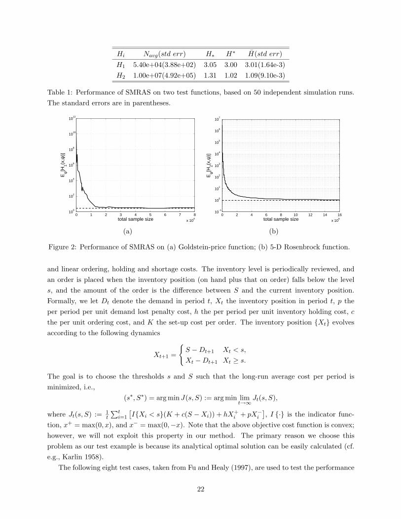
Hi Navg(std err) H∗ H∗ H(std err)
H1 5.40e+04(3.88e+02) 3.05 3.00 3.01(1.64e-3)H2 1.00e+07(4.92e+05) 1.31 1.02 1.09(9.10e-3)
Table 1: Performance of SMRAS on two test functions, based on 50 independent simulation runs.The standard errors are in parentheses.
0 1 2 3 4 5 6 7 8
x 104
100
102
104
106
108
1010
1012
total sample size
Eψ[H
1(x,ψ
)]
0 2 4 6 8 10 12 14 16
x 106
10−1
100
101
102
103
104
105
106
107
Eψ[H
2(x,ψ
)]
total sample size
(a) (b)
Figure 2: Performance of SMRAS on (a) Goldstein-price function; (b) 5-D Rosenbrock function.
and linear ordering, holding and shortage costs. The inventory level is periodically reviewed, andan order is placed when the inventory position (on hand plus that on order) falls below the levels, and the amount of the order is the difference between S and the current inventory position.Formally, we let Dt denote the demand in period t, Xt the inventory position in period t, p theper period per unit demand lost penalty cost, h the per period per unit inventory holding cost, c
the per unit ordering cost, and K the set-up cost per order. The inventory position Xt evolvesaccording to the following dynamics
Xt+1 =
S −Dt+1 Xt < s,
Xt −Dt+1 Xt ≥ s.
The goal is to choose the thresholds s and S such that the long-run average cost per period isminimized, i.e.,
(s∗, S∗) = arg minJ(s, S) := arg min limt→∞Jt(s, S),
where Jt(s, S) := 1t
∑ti=1
[IXi < s(K + c(S −Xi)) + hX+
i + pX−i
], I · is the indicator func-
tion, x+ = max(0, x), and x− = max(0,−x). Note that the above objective cost function is convex;however, we will not exploit this property in our method. The primary reason we choose thisproblem as our test example is because its analytical optimal solution can be easily calculated (cf.e.g., Karlin 1958).
The following eight test cases, taken from Fu and Healy (1997), are used to test the performance
22
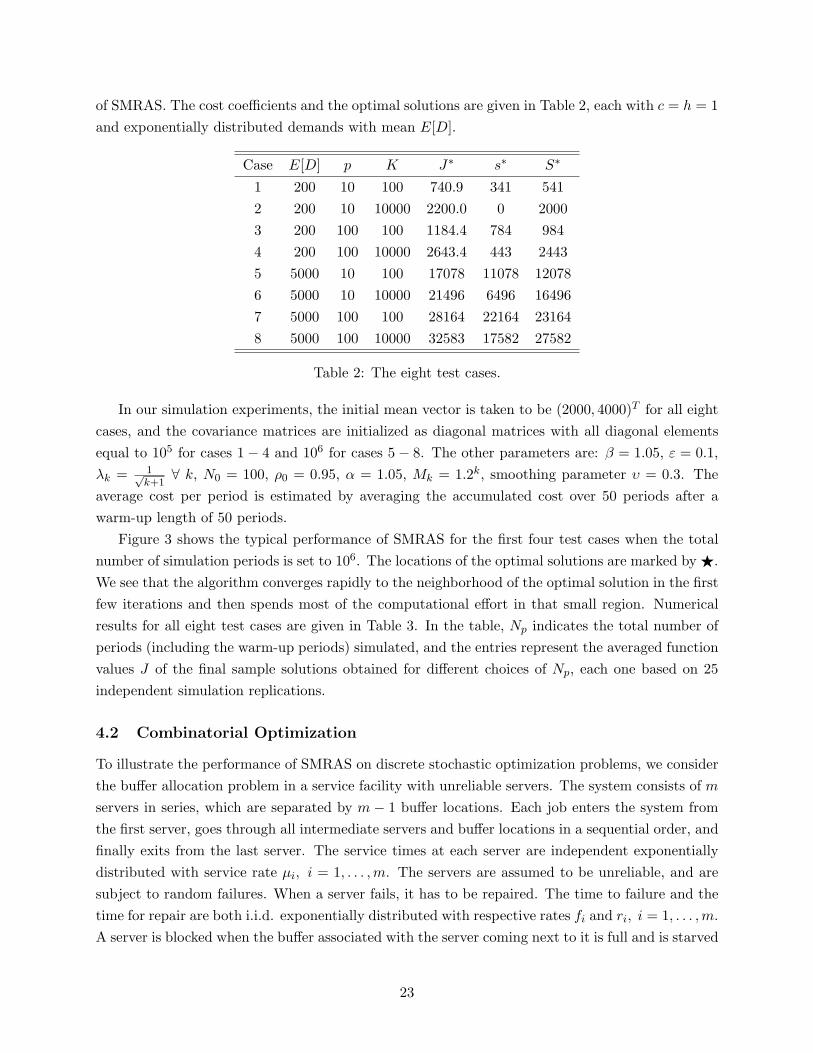
of SMRAS. The cost coefficients and the optimal solutions are given in Table 2, each with c = h = 1and exponentially distributed demands with mean E[D].
Case E[D] p K J∗ s∗ S∗
1 200 10 100 740.9 341 5412 200 10 10000 2200.0 0 20003 200 100 100 1184.4 784 9844 200 100 10000 2643.4 443 24435 5000 10 100 17078 11078 120786 5000 10 10000 21496 6496 164967 5000 100 100 28164 22164 231648 5000 100 10000 32583 17582 27582
Table 2: The eight test cases.
In our simulation experiments, the initial mean vector is taken to be (2000, 4000)T for all eightcases, and the covariance matrices are initialized as diagonal matrices with all diagonal elementsequal to 105 for cases 1− 4 and 106 for cases 5− 8. The other parameters are: β = 1.05, ε = 0.1,λk = 1√
k+1∀ k, N0 = 100, ρ0 = 0.95, α = 1.05, Mk = 1.2k, smoothing parameter υ = 0.3. The
average cost per period is estimated by averaging the accumulated cost over 50 periods after awarm-up length of 50 periods.
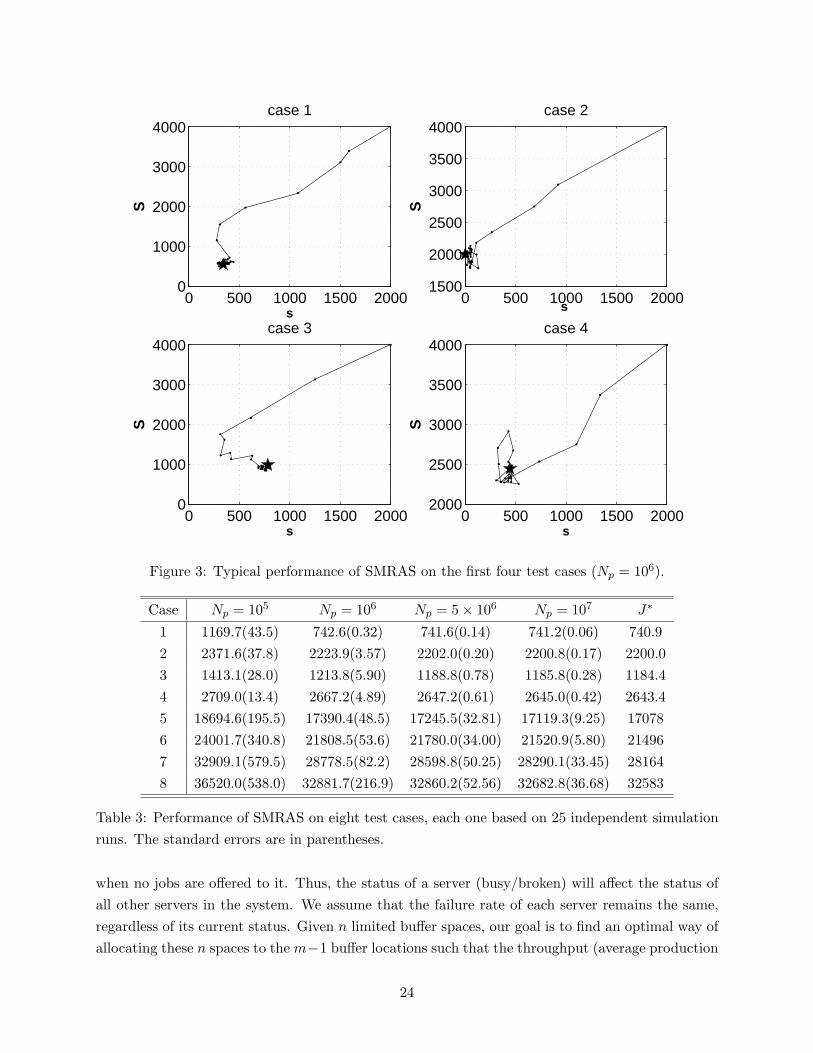
Figure 3 shows the typical performance of SMRAS for the first four test cases when the totalnumber of simulation periods is set to 106. The locations of the optimal solutions are marked by F.We see that the algorithm converges rapidly to the neighborhood of the optimal solution in the firstfew iterations and then spends most of the computational effort in that small region. Numericalresults for all eight test cases are given in Table 3. In the table, Np indicates the total number ofperiods (including the warm-up periods) simulated, and the entries represent the averaged functionvalues J of the final sample solutions obtained for different choices of Np, each one based on 25independent simulation replications.
4.2 Combinatorial Optimization
To illustrate the performance of SMRAS on discrete stochastic optimization problems, we considerthe buffer allocation problem in a service facility with unreliable servers. The system consists of m
servers in series, which are separated by m − 1 buffer locations. Each job enters the system fromthe first server, goes through all intermediate servers and buffer locations in a sequential order, andfinally exits from the last server. The service times at each server are independent exponentiallydistributed with service rate µi, i = 1, . . . , m. The servers are assumed to be unreliable, and aresubject to random failures. When a server fails, it has to be repaired. The time to failure and thetime for repair are both i.i.d. exponentially distributed with respective rates fi and ri, i = 1, . . . , m.A server is blocked when the buffer associated with the server coming next to it is full and is starved
23
0 500 1000 1500 20000
1000
2000
3000
4000S
case 1
s
0 500 1000 1500 20000
1000
2000
3000
4000
s
S
case 3
0 500 1000 1500 20002000
2500
3000
3500
4000
s
S
case 4
0 500 1000 1500 20001500
2000
2500
3000
3500
4000
s
S
case 2
Figure 3: Typical performance of SMRAS on the first four test cases (Np = 106).
Case Np = 105 Np = 106 Np = 5× 10⁶ Np = 107 J∗
1 1169.7(43.5) 742.6(0.32) 741.6(0.14) 741.2(0.06) 740.92 2371.6(37.8) 2223.9(3.57) 2202.0(0.20) 2200.8(0.17) 2200.03 1413.1(28.0) 1213.8(5.90) 1188.8(0.78) 1185.8(0.28) 1184.44 2709.0(13.4) 2667.2(4.89) 2647.2(0.61) 2645.0(0.42) 2643.45 18694.6(195.5) 17390.4(48.5) 17245.5(32.81) 17119.3(9.25) 170786 24001.7(340.8) 21808.5(53.6) 21780.0(34.00) 21520.9(5.80) 214967 32909.1(579.5) 28778.5(82.2) 28598.8(50.25) 28290.1(33.45) 281648 36520.0(538.0) 32881.7(216.9) 32860.2(52.56) 32682.8(36.68) 32583
Table 3: Performance of SMRAS on eight test cases, each one based on 25 independent simulationruns. The standard errors are in parentheses.
when no jobs are offered to it. Thus, the status of a server (busy/broken) will affect the status ofall other servers in the system. We assume that the failure rate of each server remains the same,regardless of its current status. Given n limited buffer spaces, our goal is to find an optimal way ofallocating these n spaces to the m−1 buffer locations such that the throughput (average production
24
rate) is maximized.When applying SMRAS, we have used the same technique as in Allon et al. (2005) to generate
admissible buffer allocations; the basic idea is to choose the probabilistic model as an (n + 1)-by-(m− 1) matrix P , whose (i, j)th entry specifies the probability of allocating i− 1 buffer spaces tothe jth buffer location. Please refer to their paper for a detailed discussion. Once the admissibleallocations are generated, it is straightforward to see that the entries of the matrix P are updatedat the kth iteration as
P k+1i,j =
∑Nkl=1 Sk(Hk(Xk
l ))I(Hk(Xkl ), γk+1)IXk
l,i = j∑Nk
l=1 Sk(Hk(Xkl ))I(Hk(Xk
l ), γk+1),
where Xkl , l = 1, . . . , Nk are the Nk admissible buffer allocations generated, Hk(Xk
l ) is the averagethroughput obtained via simulation when the allocation Xk
l is used, and Xkl,i = j indicates the
event that j buffer spaces are allocated to the ith buffer location (i.e., the ith element of the vectorXk
l is equal to j).For the numerical experiments, we consider two cases: (i) m = 3, n = 1, . . . , 10, µ1 = 1, µ2 =
1.2 µ3 = 1.4, failure rates fi = 0.05 and repair rates ri = 0.5 for all i = 1, 2, 3; (ii) m = 5,n = 1, . . . , 10, µ1 = 1, µ2 = 1.1, µ3 = 1.2, µ4 = 1.3, µ5 = 1.5, fi = 0.05 and ri = 0.5 for alli = 1, . . . , 5.
Apart from their combinatorial nature, an additional difficulty in solving these problems is thatdifferent buffer allocation schemes (samples) have similar performances. Thus, when only noisyobservations are available, it could be very difficult to discern the best allocation from a set ofcandidate allocation schemes. Because of this, in SMRAS we choose the performance function S(·)as an exponential function with a relatively larger base β = 10. The other parameters are as follows:ε = 0.001, λk = 0.01 ∀ k, initial sample size N0 = 10 for case (i) and N0 = 20 for case (ii), ρ = 0.9,α = 1.2, observation allocation rule Mk = (1.5)k, the stopping control parameters τ = 1e − 4 andl = 5, smoothing parameter υ = 0.7, and the initial P 0 is taken to be a uniform matrix with eachcolumn sum equal to one, i.e., P 0
i,j = 1n+1 ∀ i, j. We start all simulation replications with the
system empty. The steady-state throughputs are simulated after 100 warm-up periods, and thenaveraged over the subsequent 900 periods. Note that we have employed the sample reuse procedure(cf. Remark 1) in actual implementation of the algorithm.
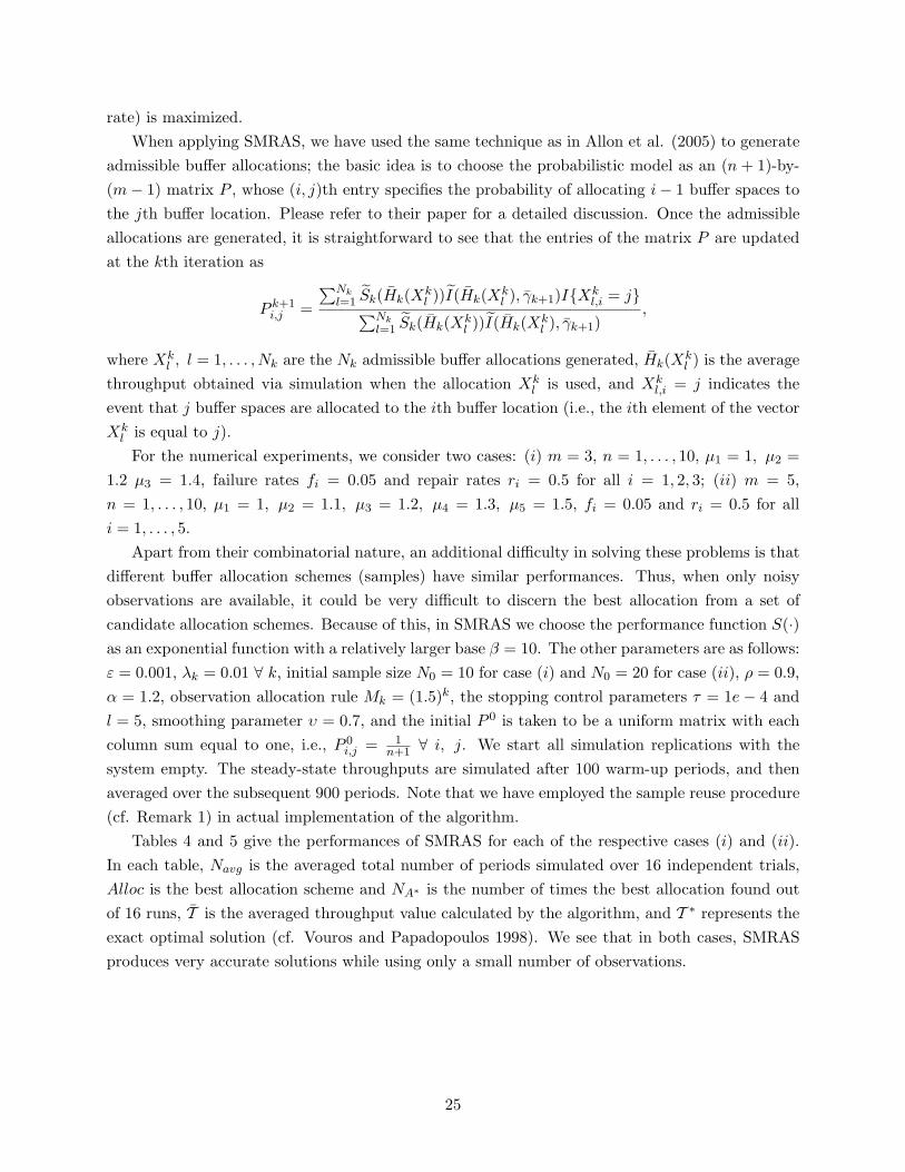
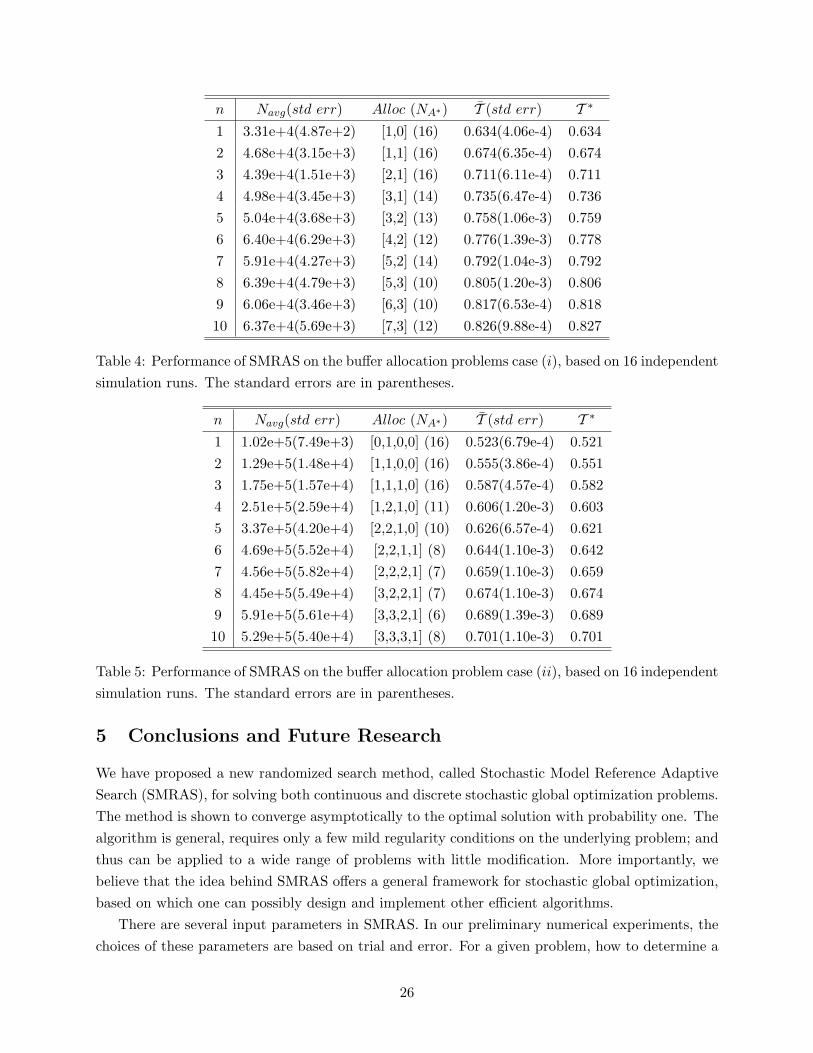
Tables 4 and 5 give the performances of SMRAS for each of the respective cases (i) and (ii).In each table, Navg is the averaged total number of periods simulated over 16 independent trials,Alloc is the best allocation scheme and NA∗ is the number of times the best allocation found outof 16 runs, T is the averaged throughput value calculated by the algorithm, and T ∗ represents theexact optimal solution (cf. Vouros and Papadopoulos 1998). We see that in both cases, SMRASproduces very accurate solutions while using only a small number of observations.
25
n Navg(std err) Alloc (NA∗) T (std err) T ∗1 3.31e+4(4.87e+2) [1,0] (16) 0.634(4.06e-4) 0.6342 4.68e+4(3.15e+3) [1,1] (16) 0.674(6.35e-4) 0.6743 4.39e+4(1.51e+3) [2,1] (16) 0.711(6.11e-4) 0.7114 4.98e+4(3.45e+3) [3,1] (14) 0.735(6.47e-4) 0.7365 5.04e+4(3.68e+3) [3,2] (13) 0.758(1.06e-3) 0.7596 6.40e+4(6.29e+3) [4,2] (12) 0.776(1.39e-3) 0.7787 5.91e+4(4.27e+3) [5,2] (14) 0.792(1.04e-3) 0.7928 6.39e+4(4.79e+3) [5,3] (10) 0.805(1.20e-3) 0.8069 6.06e+4(3.46e+3) [6,3] (10) 0.817(6.53e-4) 0.81810 6.37e+4(5.69e+3) [7,3] (12) 0.826(9.88e-4) 0.827
Table 4: Performance of SMRAS on the buffer allocation problems case (i), based on 16 independentsimulation runs. The standard errors are in parentheses.
n Navg(std err) Alloc (NA∗) T (std err) T ∗1 1.02e+5(7.49e+3) [0,1,0,0] (16) 0.523(6.79e-4) 0.5212 1.29e+5(1.48e+4) [1,1,0,0] (16) 0.555(3.86e-4) 0.5513 1.75e+5(1.57e+4) [1,1,1,0] (16) 0.587(4.57e-4) 0.5824 2.51e+5(2.59e+4) [1,2,1,0] (11) 0.606(1.20e-3) 0.6035 3.37e+5(4.20e+4) [2,2,1,0] (10) 0.626(6.57e-4) 0.6216 4.69e+5(5.52e+4) [2,2,1,1] (8) 0.644(1.10e-3) 0.6427 4.56e+5(5.82e+4) [2,2,2,1] (7) 0.659(1.10e-3) 0.6598 4.45e+5(5.49e+4) [3,2,2,1] (7) 0.674(1.10e-3) 0.6749 5.91e+5(5.61e+4) [3,3,2,1] (6) 0.689(1.39e-3) 0.68910 5.29e+5(5.40e+4) [3,3,3,1] (8) 0.701(1.10e-3) 0.701
Table 5: Performance of SMRAS on the buffer allocation problem case (ii), based on 16 independentsimulation runs. The standard errors are in parentheses.
5 Conclusions and Future Research
We have proposed a new randomized search method, called Stochastic Model Reference AdaptiveSearch (SMRAS), for solving both continuous and discrete stochastic global optimization problems.The method is shown to converge asymptotically to the optimal solution with probability one. Thealgorithm is general, requires only a few mild regularity conditions on the underlying problem; andthus can be applied to a wide range of problems with little modification. More importantly, webelieve that the idea behind SMRAS offers a general framework for stochastic global optimization,based on which one can possibly design and implement other efficient algorithms.
There are several input parameters in SMRAS. In our preliminary numerical experiments, thechoices of these parameters are based on trial and error. For a given problem, how to determine a
26
priori the most appropriate values of these parameters is an open issue. One research topic is tostudy the effects of these parameters on the performance of the method, and possibly design anadaptive scheme to choose these parameters adaptively during the search process.
Our current numerical study with the algorithm shows that the objective function need not beevaluated very accurately during the initial search phase. Instead, it is sufficient to provide thealgorithm with a rough idea where the good solutions are located. This has motivated our researchto use observation allocation rules with adaptive increasing rates during different search phases.For instance, during the initial search phase, we could increase Mk at a linear rate or even keepit at a constant value; and exponential rates will only be used during the later search phase whenmore accurate estimates of the objective function values are required.
Some other research topics that would further enhance of the performance of SMRAS includeincorporating local search techniques in the algorithm and implementing a paralleled version of themethod.
References
G. Allon, D. P. Kroese, T. Raviv, and R. Y. Rubinstein 2005. “Application of the cross-entropymethod to the buffer alloation problem in a simulation-based environment,” Annals of OperationsResearch, Vol. 134, pp. 137-151.
M. H. Alrefaei and S. Andradottir 1995. “A modification of the stochastic ruler method for discretestochastic optimization,” European Journal of Operational Research, Vol. 133, pp. 160-182.
M. H. Alrefaei and S. Andradottir 1999. “A simulated annealing algorithm with constant temper-ature for discrete stochastic optimization,” Management Science, Vol. 45, pp. 748-764.
S. Andradottir 1995. “A method for discrete stochastic optimization,” Management Science, Vol.41, pp. 1946-1961.
P. T. De Boer, D. P. Kroese, S. Mannor, R. Y. Rubinstein 2005. “A tutorial on the cross-entropymethod,” Annals of Operation Research, Vol. 134, pp. 19-67.
M. Dorigo and L. M. Gambardella 1997. “Ant colony system: a cooperative learning approach tothe traveling salesman problem,” IEEE Trans. on Evolutionary Computation, Vol. 1, pp. 53-66.
M. C. Fu and K. J. Healy 1997. “Techniques for simulation optimization: an experimental studyon an (s, S) inventory system,” IIE Transactions, Vol. 29, pp. 191-199.
M. C. Fu 2005. Stochastic gradient estimation. Chapter 19 in Handbooks in Operations Researchand Management Science: Simulation, S.G. Henderson and B.L. Nelson, eds., Elsevier, 2005.
W. J. Gutjahr 2003. “A converging ACO algorithm for stochastic combinatorial optimization,”Proc. SAGA 2003 Stochastic Algorithms: Foundations and Applications, Hatfield (UK), A. Al-brecht, K. Steinhoefl, eds., Springer LNCS 2827 10− 25.
27
W. Hoeffding 1963. “Probability inequalities for sums of bounded random variables,” Journal ofthe American Statistical Association, Vol. 58, pp. 13-30.
L. J. Hong and B. L. Nelson 2005. “Discrete optimization via simulation using COMPASS,”Operations Research, forthcoming.
J. Hu, M. C. Fu, and S. I. Marcus 2005. “A model reference adaptive search algorithm for globaloptimization,” Operations Research, submitted.
R. Y. Rubinstein 1999. “The cross-entropy method for combinatorial and continuous optimization,”Methodology and Computing in Applied Probability, Vol. 2, pp. 127-190.
R. Y. Rubinstein 2001. “Combinatorial optimization, ants and rare events,” Stochastic Optimiza-tion: Algorithms and Applications, 304− 358, S. Uryasev and P. M. Pardalos, eds., Kluwer.
R. Y. Rubinstein and D. P. Kroese 2004. The cross-entropy method: a unified approach to combi-natorial optimization, Monte-Carlo simulation, and machine learning. Springer, New York.
L. Shi and S. Olafsson 2000. “Nested partitions method for stochastic optimization,” Methodologyand Computing in Applied Probability, Vol. 2, pp. 271-291.
G. A. Vouros and H. T. Papadopoulos 1998. “Buffer allocation in unreliable production lines usinga knowledge based system,” Computer & Operations Research, Vol. 25, pp. 1055-1067.
D. Yan and H. Mukai 1992. “Stochastic discrete optimization,” SIAM Journal on Control andOptimization, Vol. 30, pp. 594-612.
M. Zlochin, M. Birattari, N. Meuleau, and M. Dorigo 2001. “Model-based search for combinatorialoptimization,” Annals of Operations Research, Vol. 131, pp. 373-395.
28
Appendix
Proof of Lemma 3.2: For the same reason as discussed in the proof of Lemma 2.1, we onlyneed to consider the case where
x : Hk(x) > γk+1 − ε, x ∈ Xk
1 , . . . , XkNk 6= ∅. Define
Jk(θ) =1
Nk
Nk∑
i=1
Sk(Hk(Xki ))I
(Hk(Xk
i ), γk+1
)ln f(Xk
i , θ), where Sk(Hk(x)) := [S(Hk(x))]k
f(x,θk).
Since f(·, θ) belongs to the NEF, we can write
Jk(θ) =1
Nk
Nk∑
i=1
Sk(Hk(Xki ))I
(Hk(Xk
i ), γk+1
)ln `(Xk
i )
+1
Nk
Nk∑
i=1
Sk(Hk(Xki ))I
(Hk(Xk
i ), γk+1
)θT Γ(Xk
i )
− 1Nk
Nk∑
i=1
Sk(Hk(Xki ))I
(Hk(Xk
i ), γk+1
)ln
∫
x∈XeθT Γ(x)`(x)ν(dx).
Thus the gradient of Jk(θ) with respect to θ can be expressed as
∇θJk(θ) =1
Nk
Nk∑
i=1
Sk(Hk(Xki ))I
(Hk(Xk
i ), γk+1
)Γ(Xk
i )
−∫
eθT Γ(x)Γ(x)`(x)ν(dx)∫eθT Γ(x)`(x)ν(dx)
1Nk
Nk∑
i=1
Sk(Hk(Xki ))I
(Hk(Xk
i ), γk+1
),
where the validity of the interchange of derivative and integral above is guaranteed by AssumptionA6 and the dominated convergence theorem. By setting ∇θJk(θ) = 0, it follows that
1Nk
∑Nki=1 Sk(Hk(Xk
i ))I(Hk(Xk
i ), γk+1
)Γ(Xk
i )1
Nk
∑Nki=1 Sk(Hk(Xk
i ))I(Hk(Xk
i ), γk+1
) =∫
eθT Γ(x)Γ(x)`(x)ν(dx)∫eθT Γ(x)`(x)ν(dx)
,
which implies that Egk+1[Γ(X)] = Eθ [Γ(X)] by the definitions of gk(·) (cf. (4)) and f(·, θ).
Since θk+1 is the optimal solution of the problem
argmaxθ∈Θ
Jk(θ),
we conclude that Egk+1[Γ(X)] = Eθk+1
[Γ(X)] , ∀ k = 0, 1, . . ., by A5.
Proof of Lemma 3.3: Our proof is an extension of Hu et al. (2005). Let Ω1 be the set of allsample paths such that step 3a/3b is visited finitely often, and let Ω2 be the set of sample pathssuch that limk→∞h(x) ≥ γk − ε ⊆ Π. By Lemma 3.1, we have P (Ω1) = 1, and for each ω ∈ Ω1,there exists a finite N (ω) > 0 such that
X†k+1(ω) = X†
k(ω) ∀ k ≥ N (ω),
29
which implies that γk+1(ω) = γk(ω) ∀ k ≥ N (ω). Furthermore, by A1, we have P (Ω2) = 1 andh(x) ≥ γk(ω)− ε ⊆ Π, ∀ k ≥ N (ω) ∀ω ∈ Ω1 ∩ Ω2.
Thus, for each ω ∈ Ω1 ∩ Ω2, it is not difficult to see from equation (6) that gk+1(·) can beexpressed recursively as
gk+1(x) =S(h(x))gk(x)Egk
[S(h(X))], ∀ k > N (ω),
where we have used gk(·) instead of gk(ω)(·) to simplify the notation. It follows that
Egk+1[S(h(X))] =
Egk[S2(h(X))]
Egk[S(h(X))]
≥ Egk[S(h(X))] , ∀ k > N (ω), (10)
which implies that the sequence Egk[h(X)], k = 1, 2, . . . converges (note that Egk
[h(X)] is boundedfrom above by h(x∗)).
Now we show that the limit of the above sequence is S(h(x∗)). To show this, we proceed bycontradiction and assume that
limk→∞
Egk[S(h(X))] = S∗ < S∗ := S(h(x∗)).
Define the set C := x : h(x) ≥ γN (ω) − ε ∩ x : S(h(x)) ≥ S∗+S∗2 ∩ X . Since S(·) is strictly
increasing, its inverse S−1(·) exists, thus C can be formulated as C =x : h(x) ≥ maxγN (ω) −
ε, S−1(S∗+S∗2 ) ∩ X . By A2, C has a strictly positive Lebesgue/discrete measure.
Note that gk+1(·) can be written as
gk+1(x) =k∏
i=N (ω)+1
S(h(x))Egi [S(h(X))]
· gN (ω)+1(x), ∀ k > N (ω).
Since limk→∞S(h(x))
Egk[S(h(X))] = S(h(x))
S∗ > 1, ∀ x ∈ C, we conclude that
lim infk→∞
gk(x) = ∞, ∀ x ∈ C.
We have, by Fatou’s lemma,
1 = lim infk→∞
∫
Xgk+1(x)ν(dx) ≥ lim inf
k→∞
∫
Cgk+1(x)ν(dx) ≥
∫
Clim infk→∞
gk+1(x)ν(dx) = ∞,
which is a contradiction. Hence, it follows that
limk→∞
Egk[S(h(X))] = S∗, ∀ ω ∈ Ω1 ∩ Ω2. (11)
We now bound the difference between Egk+1[Γ(X)] and Γ(x∗). We have
‖Egk+1[Γ(X)]− Γ(x∗)‖ ≤
∫
x∈X‖Γ(x)− Γ(x∗)‖gk+1(x)ν(dx)
=∫
D‖Γ(x)− Γ(x∗)‖gk+1(x)ν(dx), (12)
where D :=x : h(x) ≥ γN (ω) − ε
∩ X is the support of gk+1(x), ∀ k > N (ω).
30
By the assumption on Γ(·) in Definition 3.1, for any given ζ > 0, there exists a δ > 0 such that‖x− x∗‖ ≤ δ implies ‖Γ(x)− Γ(x∗)‖ ≤ ζ. Let Aδ be defined as in A3; then we have from (12)
‖Egk+1[Γ(X)]− Γ(x∗)‖ ≤
∫
Acδ∩D
‖Γ(x)− Γ(x∗)‖gk+1(x)ν(dx) +∫
Aδ∩D‖Γ(x)− Γ(x∗)‖gk+1(x)ν(dx)
≤ ζ +∫
Aδ∩D‖Γ(x)− Γ(x∗)‖gk+1(x)ν(dx), ∀ k > N (ω). (13)
The rest of the proof amounts to showing that the second term in (13) is also bounded. Clearlyby A1, the term ‖Γ(x) − Γ(x∗)‖ is bounded on the set Aδ ∩ D. We only need to find a bound forgk+1(x).
By A3, we havesup
x∈Aδ∩Dh(x) ≤ sup
x∈Aδ
h(x) < h(x∗).
Define Sδ := S∗ − S(supx∈Aδh(x)). And by the monotonicity of S(·), we have Sδ > 0. It is easy to
see thatS(h(x)) ≤ S∗ − Sδ, ∀x ∈ Aδ ∩ D. (14)
From (10) and (11), there exists N (ω) ≥ N (ω) such that for all k ≥ N (ω)
Egk+1[S(h(X))] ≥ S∗ − 1
2Sδ. (15)
Observe that gk+1(x) can be rewritten as
gk+1(x) =k∏
i=N
S(h(x))Egi [S(h(X))]
· gN (x), ∀ k ≥ N (ω).
Thus, it follows from (14) and (15) that
gk+1(x) ≤( S∗ − Sδ
S∗ − 12Sδ
)k−N+1· gN (x), ∀x ∈ Aδ ∩ D, ∀ k ≥ N (ω).
Therefore,
‖Egk+1[Γ(X)]− Γ(x∗)‖ ≤ ζ + sup
x∈Aδ∩D‖Γ(x)− Γ(x∗)‖
∫
Aδ∩Dgk+1(x)ν(dx)
≤ ζ + supx∈Aδ∩D
‖Γ(x)− Γ(x∗)‖( S∗ − Sδ
S∗ − 12Sδ
)k−N+1, ∀ k ≥ N (ω)
≤(1 + sup
x∈Aδ∩D‖Γ(x)− Γ(x∗)‖
)ζ, ∀ k ≥ N (ω),
where N (ω) is given by N (ω) := maxN (ω), dN (ω)− 1 + ln ζ/ ln
(S∗−Sδ
S∗− 12Sδ
)e.
Since ζ is arbitrary, we have
limk→∞
Egk[Γ(X)] = Γ(x∗), ∀ω ∈ Ω1 ∩ Ω2.
And since P (Ω1 ∩ Ω2) = 1, the proof is thus completed.
31

Proof of Proposition 3.1: Again, we consider the sequenceX†
k
generated by SMARS. We
have for any ζ > 0
P(∣∣γk+1 − γk+1
∣∣ ≥ ζ
αk
)= P
(∣∣Hk(X†k+1)− h(X†
k+1)∣∣ ≥ ζ
αk
)
≤⋃
x∈Λk
P(∣∣Hk(x)− h(x)
∣∣ ≥ ζ
αk
)
≤∑
x∈Λk
P(∣∣Hk(x)− h(x)
∣∣ ≥ ζ
αk
)
≤ ∣∣Λk
∣∣ supx∈X
P(∣∣Hk(x)− h(x)
∣∣ ≥ ζ
αk
)
≤ αkN0φ(Mk, ζ/αk) by L1
≤ N0(δ∗)k ∀ k ≥ K by L4 and the definition of φ(·, ·).
Thus ∞∑
k=1
P(∣∣γk+1 − γk+1
∣∣ ≥ ζ
αk
)≤ K + N0
∞∑
k=K(δ∗)k < ∞.
And by Borel-Cantelli lemma,
P(∣∣γk+1 − γk+1)
∣∣ ≥ ζ
αk
i.o.
)= 0.
Let Ω1 be defined as before, and define Ω3 :=ω : αk |γk+1 − γk+1| ≥ ζ i.o.
. Since for each ω ∈ Ω1,
there exists a finite N (ω) > 0 such that γk+1(ω) = γk(ω) ∀ k ≥ N (ω), we have
P(αk
∣∣γk+1 − γk
∣∣ ≥ ζ i.o.)
= P(∣∣γk+1 − γk
∣∣ ≥ ζ
αki.o. ∩ Ω1
)+ P
(∣∣γk+1 − γk
∣∣ ≥ ζ
αki.o. ∩ Ωc
1
)
≤ P (Ω3 ∩ Ω1) + P (Ωc1)
= 0.
And since ζ is arbitrary, the proof is thus completed.
32