Embed Size (px)
Citation preview

A MODULAR REWRITING APPROACH TO
LANGUAGE DESIGN, EVOLUTION AND ANALYSIS
Mark Hills
To cite this version:
Mark Hills. A MODULAR REWRITING APPROACH TO LANGUAGE DESIGN, EVOLU-TION AND ANALYSIS. Software Engineering [cs.SE]. University of Illinois at Urbana Cham-paign, 2009. English. <tel-00535886>
HAL Id: tel-00535886
https://tel.archives-ouvertes.fr/tel-00535886
Submitted on 13 Nov 2010
HAL is a multi-disciplinary open accessarchive for the deposit and dissemination of sci-entific research documents, whether they are pub-lished or not. The documents may come fromteaching and research institutions in France orabroad, or from public or private research centers.
L’archive ouverte pluridisciplinaire HAL, estdestinee au depot et a la diffusion de documentsscientifiques de niveau recherche, publies ou non,emanant des etablissements d’enseignement et derecherche francais ou etrangers, des laboratoirespublics ou prives.

A MODULAR REWRITING APPROACH TO LANGUAGE
DESIGN, EVOLUTION AND ANALYSIS
BY
MARK A. HILLS
DISSERTATION
Submitted in partial fulfillment of the requirements
for the degree of Doctor of Philosophy in Computer Science
in the Graduate College of the
University of Illinois at Urbana-Champaign, 2009
Urbana, Illinois
Doctoral Committee:
Associate Professor Grigore Rosu, Chair and Director of Research
Professor Carl Gunter
Associate Professor Samuel N Kamin
Professor Jose Meseguer
Professor Peter D Mosses, Swansea University

Abstract
Software is becoming a pervasive presence in our lives, powering computing
systems in the home, in businesses, and in safety-critical settings. In response,
languages are being defined with support for new domains and complex compu-
tational abstractions. The need for formal techniques to help better understand
the languages we use, correctly design new language abstractions, and reason
about the behavior and correctness of programs is now more urgent then ever.
In this dissertation we focus on research in programming language semantics
and program analysis, aimed at building and reasoning about programming
languages and applications. In language semantics, we first show how to use
formal techniques during language design, presenting definitional techniques for
object-oriented languages with concurrency features, including the Beta language
and a paradigmatic language called KOOL. Since reuse is important, we then
present a module system for K, a formalism for language definition that takes
advantage of the strengths of rewriting logic and term rewriting techniques.
Although currently specific to K, parts of this module system are also aimed at
other formalisms, with the goal of providing a reuse mechanism for different forms
of modular semantics in the future. Finally, since performance is also important,
we show techniques for improving the executable and analysis performance of
rewriting logic semantics definitions, specifically focused on decisions around the
representation of program values and configurations used in semantics definitions.
The work on performance, with a discussion of analysis performance, provides
a good bridge to the second major topic, program analysis. We present a new
technique aimed at annotation-driven static analysis called policy frameworks. A
policy framework consists of analysis domains, an analysis generic front-end, an
analysis-generic abstract language semantics, and an abstract analysis semantics
that defines the semantics of the domain and the annotation language. After
illustrating the technique using SILF, a simple imperative language, we then
describe a policy framework for C. To provide a real example of using this
framework, we have defined a units of measurement policy for C. This policy
allows both type and code annotations to be added to standard C programs,
which are then used to generate modular analysis tasks checked using the CPF
semantics in Maude.
ii

To Sally.
iii

Acknowledgments
During the time I have been working on my dissertation I have had the good
fortune to work with a number of outstanding people, both at the University of
Illinois at Urbana-Champaign and in the broader research community.
I would first like to acknowledge all the support I’ve received over the years
from my advisor, Grigore Rosu. He has been a friend and a mentor, and his
influence can be found throughout this dissertation. The environment he has
provided in the Formal Systems Laboratory has been challenging (in the best
sense), intellectually stimulating, and fun, as all good research should be. I look
forward to continuing our collaboration in the future.
I would also like to thank the rest of my thesis committee, made up of Carl
Gunter, Sam Kamin, Jose Meseguer, and Peter Mosses. Their experience and
input have been important to improving the quality of this research, with advice
on not just where to focus, but, sometimes even more importantly, on where not
to focus, helping me to avoid going down blind alleys. Also, their time reading,
and rereading, various parts of the thesis, offering criticism and advice, has
helped to make this thesis much better than it otherwise would have been.
Next, I would like to thank my fellow current and former Formal Systems Lab-
mates, Feng Chen, Marcelo d’Amorim, Chucky Ellison, Dongyun Jin, Choongh-
wan Lee, Patrick Meredith, Andrei Popescu, and Traian Serbanuta, with whom
I spent many hours (days? years?) discussing programming languages, rewriting
logic, various semantics frameworks, static analysis, how to pronounce words in
Romanian, and many other topics. They have all made FSL a fun, collaborative,
and always interesting place to do research.
A number of people at the University of Illinois, but outside of my committee
and research group, have also had an impact on this research and, more generally,
my time in graduate school. Thanks to Steven Lauterberg for many interesting
conversations; to Baris Aktemur, for discussions about research, joining me
in fighting various tools on the way to finishing class projects, and getting
involved with me in defining the semantics of Beta, a wonderful language that is,
unfortunately, more widely known than used; and Ralf Sasse, for wide-ranging
discussions on everything from research to (American) football to the incredible
length of German words.
Thanks also to Elsa Gunter, for providing wonderful advise about research
iv

and teaching, for offering interesting courses, and for helping me find parking
in Hyde Park on a Saturday; and to the various support people here in the
department, whose helpfulness and kindness to me and my family have made
the experience here all the better.
Moving beyond UIUC, I would like to thank, in general, the many students
and researchers at other institutions that I have encountered over the last several
years, and specifically, Jonathan Aldrich, Andrew Black, Erik Ernst, Jeremy
Siek, and Carolyn Talcott, who have all given me advise, in formal or informal
settings, during the time I’ve been working on my dissertation.
Finally, I would like to thank my family. My parents, Clinton and Linda Hills,
and my in-laws, Fred and Elaine Longacre, have all encouraged me throughout
this process. My daughter Rebecca was born the same day I was admitted into
the graduate program, and has been a joy to watch as she’s grown during my
time at UIUC. My son Matthew decided to arrive a month early, on the night
of a paper deadline, and, outside of that initial inconsiderate act (your sister
was born on her due date, Matthew...), his sunny disposition has brightened the
house. Of course, none of this would have been possible without my wife Sally,
whose patience, encouragement, help, and love have been indispensible.
The research in this dissertation has been supported in part by NSF grants
CCF-0448501, CNS-0509321 and CNS-0720512, by NASA contract NNL08AA23C,
by the Microsoft/Intel funded Universal Parallel Computing Research Center at
UIUC, and by several Microsoft gifts.
v
Table of Contents
Chapter 1 Introduction . . . . . . . . . . . . . . . . . . . . . . . . 1
1.1 Contributions . . . . . . . . . . . . . . . . . . . . . . . . . . . . . 21.2 An Overall Guide to the Thesis . . . . . . . . . . . . . . . . . . . 41.3 Relationship to Previous Work . . . . . . . . . . . . . . . . . . . 41.4 Related Publications . . . . . . . . . . . . . . . . . . . . . . . . . 5
Chapter 2 Background . . . . . . . . . . . . . . . . . . . . . . . . 7
2.1 Equational Logic . . . . . . . . . . . . . . . . . . . . . . . . . . . 72.2 Term Rewriting . . . . . . . . . . . . . . . . . . . . . . . . . . . . 122.3 Rewriting Logic . . . . . . . . . . . . . . . . . . . . . . . . . . . . 142.4 Rewriting Logic Semantics . . . . . . . . . . . . . . . . . . . . . . 172.5 K . . . . . . . . . . . . . . . . . . . . . . . . . . . . . . . . . . . . 22
Chapter 3 Language Prototyping . . . . . . . . . . . . . . . . . . 31
3.1 Introducing KOOL . . . . . . . . . . . . . . . . . . . . . . . . . . 323.2 Abstract Syntax . . . . . . . . . . . . . . . . . . . . . . . . . . . 353.3 State Infrastructure and Value Representations . . . . . . . . . . 413.4 Dynamic Semantics . . . . . . . . . . . . . . . . . . . . . . . . . . 443.5 Adding Concurrency . . . . . . . . . . . . . . . . . . . . . . . . . 533.6 Other Extensions . . . . . . . . . . . . . . . . . . . . . . . . . . . 573.7 KOOL Implementation . . . . . . . . . . . . . . . . . . . . . . . . 61
Chapter 4 A Prototype of Beta . . . . . . . . . . . . . . . . . . 63
4.1 The Beta Language . . . . . . . . . . . . . . . . . . . . . . . . . . 634.2 Beta Semantics . . . . . . . . . . . . . . . . . . . . . . . . . . . . 644.3 Beta Implementation . . . . . . . . . . . . . . . . . . . . . . . . . 694.4 Extending Beta . . . . . . . . . . . . . . . . . . . . . . . . . . . . 69
Chapter 5 The K Module System . . . . . . . . . . . . . . . . . . 71
5.1 K Modules . . . . . . . . . . . . . . . . . . . . . . . . . . . . . . 735.2 Module Examples . . . . . . . . . . . . . . . . . . . . . . . . . . . 795.3 An Extended Example: Creating Language Extensions . . . . . . 825.4 Translating K Modules to Maude . . . . . . . . . . . . . . . . . . 955.5 The Online Semantics Repository . . . . . . . . . . . . . . . . . . 965.6 Discussion . . . . . . . . . . . . . . . . . . . . . . . . . . . . . . . 100
Chapter 6 Language Design and Performance . . . . . . . . . . 103
6.1 Execution Performance . . . . . . . . . . . . . . . . . . . . . . . . 1036.2 Analysis Performance . . . . . . . . . . . . . . . . . . . . . . . . 114
Chapter 7 Policy Frameworks . . . . . . . . . . . . . . . . . . . 120
7.1 Abstract Analysis Domains . . . . . . . . . . . . . . . . . . . . . 1227.2 The SILF Policy Framework . . . . . . . . . . . . . . . . . . . . . 125
vi

Chapter 8 The C Policy Framework . . . . . . . . . . . . . . . 134
8.1 CPF Frontend and Annotation Support . . . . . . . . . . . . . . 1348.2 Abstract Syntax . . . . . . . . . . . . . . . . . . . . . . . . . . . 1388.3 K Cells . . . . . . . . . . . . . . . . . . . . . . . . . . . . . . . . 1388.4 Abstract Evaluation Semantics . . . . . . . . . . . . . . . . . . . 1408.5 The CPF UNITS Policy . . . . . . . . . . . . . . . . . . . . . . . 1448.6 Case Study: Null Pointer Analysis . . . . . . . . . . . . . . . . . 1518.7 Discussion . . . . . . . . . . . . . . . . . . . . . . . . . . . . . . . 154
Chapter 9 Related Work . . . . . . . . . . . . . . . . . . . . . . 156
9.1 Programming Language Semantics . . . . . . . . . . . . . . . . . 1569.2 Program Analysis . . . . . . . . . . . . . . . . . . . . . . . . . . . 188
Chapter 10 Conclusions and Future Work . . . . . . . . . . . . 192
References . . . . . . . . . . . . . . . . . . . . . . . . . . . . . . . . 195
vii
Chapter 1
Introduction
Software is a pervasive presence in our lives. Computers are now a common
feature in homes and businesses, while smaller computers, known as embedded
systems, are now found in everything from household appliances to phones to
automobiles and airplanes. With the need for software growing, new languages
are being defined to meet new development challenges. These language often
include support for complex abstractions, and are targeted at challenging domains
such as families of configurable software products and ultra-large scale systems
made up of distributed software components. Even in home computing systems,
Internet connections and multi-core processors are now common, making once
more academic concerns, such as concurrency and distributed computing, into
concerns for regular application developers and game designers.
The pervasive nature of computation unfortunately has its downsides: com-
puter failures can now be quite costly. This is often just measured in monetary
costs: the loss of the NASA Mars Climate Orbiter due to a simple (yet hard to
catch) programming error [2] resulted in a loss of 327.6 million dollars between
the cost of the orbiter and associated lander [3]. Some software errors have led
to consequences more serious than just loss of money: errors in the software
used to control the Therac-25 radiation therapy machine [114] led to six known
accidents, causing serious injuries and, in three cases, death.
The research described in this thesis is aimed around a core motivating
concept: with the increased complexity of programming languages and software
systems, along with the pervasive presence of software in everyday devices and
safety-critical systems, the need for formal techniques to help better understand
the languages we use, correctly design new language abstractions, and reason
about the behavior and correctness of programs is more urgent then ever. One
branch of this research is focused on programming language semantics, specifi-
cally on improving the ability to formally design new programming languages
and extend existing languages with new features. The second branch of the
research described herein is focused on program analysis and program verifica-
tion, specifically on using semantics-driven techniques to find errors in programs
and/or show that they are correct in regards to a given specification.
Unfortunately, formal techniques for defining the semantics of a programming
language have not been very successful outside the research community, and
1

often are not used even inside the research community [145, 149]. An overall
goal across both branches of this research is to contribute to changing this, by
providing better ways to define language features, reuse defined features across
languages, and analyze programs based on a given language semantics.
1.1 Contributions
The research described in this thesis makes the following key contributions:
1. This thesis gives the first rewriting logic semantics and K definitions
of a number of complex features found in real programming languages,
including Smalltalk-like primitive operations (used to perform operations
such as arithmetic or value comparisons in pure object-oriented languages
without scalars), Beta-style inner calls, auto-boxing of scalars into objects,
coroutines, and garbage collection. This research is described in detail in
Chapters 3, 4, and 6.
2. Current K tool support requires language feature definitions to be manually
assembled into a single module before use. This thesis introduces a module
system for K, providing a mechanism to build modules containing reusable
language features, and including novel features designed for making def-
initions more concise and for working with different kinds of semantics
(standard dynamic and static semantics, semantics aimed at program
analysis, etc.). The module system also includes additional functionality
for sharing modules between different tools and over the Internet, with a
shared module repository. This research is described further in Chapter 5
3. To improve the flexibility of program analysis frameworks, we introduce
policy frameworks, the first mechanism to define generic, modular analysis
frameworks with a focus on reuse both within a single language and
(without a translation into a shared intermediate language) across multiple
languages. As a proof of concept, we also introduce the C Policy Framework,
including a policy for checking the proper usage of units of measurement,
the UNITS policy. This policy is competitive with existing state of the art
tools for checking for unit safety, with good performance and an annotation
language more expressive than those provided by any other annotation-
based unit checker of which we are aware. It also achieves a large amount of
reuse, with a significant portion of the definition shared with other policies
in CPF and with the units domain shared with policy frameworks for other
languages. Policy frameworks are described in more detail in Chapter 7,
while the C Policy Framework and the UNITS policy are described further
in Chapter 8.
The contributions listed above have primarily been driven by this author,
although all are to some extent collaborative. The basis for this work has been
2

the computation-based style of rewriting logic semantics and K (described more
in Chapter 2), developed by Grigore Rosu. The definition of Beta has been a
joint effort with Barıs Aktemur, while some of the core research directions for
policy frameworks and the UNITS policy were developed in collaboration with
Grigore Rosu and Feng Chen. Work on the module system has involved close
cooperation with Grigore Rosu; Traian Florin Serbanuta who has been working
on the K Tools developed in Maude; and Chucky Ellison, who developed an
initial (non-modular) toolset for working with K and is an active user of the new
module system.
Broader Impact: The broader impact of these contributions is in the following
areas:
1. Research into defining complex language features using K benefits both
language designers and other researchers in language semantics, providing
definitions which can be used directly during language prototyping and for
guidance when defining new, but similar, features.
2. Research into the K module system makes some initial steps towards having
a shared repository of reusable language features, a goal not just for K but
for other styles of semantics as well (such as the work on Component-Based
Semantics, discussed in Chapter 9). It also makes the work on K more
accessible to others, providing, as the repository is loaded, a number of
pre-built and pre-tested features which are ready to be used when building
language definitions.
3. Research on policy frameworks provides a general method for adding
reusable analysis frameworks to languages, hopefully moving the creation
of analysis tools away from highly focused tools that are not reusable or
extensible and allowing semantics-based analysis frameworks to be added
more easily to a language. The work on policy frameworks is also currently
acting as a springboard for work on proving properties of programs in a
modular fashion.
As mentioned above, one goal of this research is to increase the use of formal
techniques in language design. It is hoped that, by providing tools and techniques
which can be used to prototype even complex languages; ways to leverage these
definitions for program analysis; and tool support for working with existing
feature definitions, the research outlined in this thesis will lead to an increased
use of formal techniques (in general) and K (specifically) for language design.
It is also hoped that the work on the module repository, including a standard
exchange format for language feature definition modules and tool support for
both interacting with the repository and combining modules, will also be useful
for modular semantics formalisms other than K, such as MSOS, Action Semantics,
or Monads.
3

1.2 An Overall Guide to the Thesis
Chapter 2 provides a brief introduction to some background material that is
helpful to understanding the remainder of the thesis: term rewriting systems,
equational and rewriting logic, rewriting logic semantics, and K.
Chapters 3, 4, and 5 are focused on language semantics: Chapter 3 discusses
language prototyping in the context of the KOOL language, while Chapter 4
widens this discussion to include features of the Beta programming language.
Chapter 5 then provides details on the K module system, including an online
module repository designed to hold not only K modules, but modules defined in
other formalisms as well.
Chapters 6, 7, and 8 are focused on program analysis. Chapter 6 acts as a
bridge of sorts, tying some of the work on language design in with both execution
and analysis performance. Chapter 7 then introduces the concept of policy
frameworks, using the SILF language as an illustrative example. The C Policy
Framework, built around the same principles as the policy framework for SILF,
but with a much more complex language and a keener focus on performance, is
then described in Chapter 8.
The next chapter, Chapter 9, discusses related work, especially focusing on
work in tool-supported semantics, definitional modularity, and program analysis.
An in-depth comparison of K with other formalisms is not presented, but is itself
the topic of a fair portion of the current K report [167]. The thesis then ends
with conclusions and a discussion of planned and possible future research based
on the topics presented in this thesis, found in Chapter 10. Cited references are
included at the end of the thesis.
1.3 Relationship to Previous Work
The work on rewriting logic semantics and K has similar goals to other work on
language semantics – providing a means to define and reason about programming
languages and their programs. One goal of this research has been to overcome
some of the shortcomings we found in other formalisms, while taking advantage
of the algebraic setting provided by rewriting logic. A specific goal has been
to create modular definitions made up of reusable pieces, a goal shared by a
number of other formalisms, such as MSOS, Action Semantics, Monads, and
(with Montages) Abstract State Machines. This has driven features of K, such as
context transformers (described in Chapter 2), and features of the module system
(described in Chapter 5). A comparison of this work on language prototyping
and modularity with similar work in other formalisms is provided in Chapter 9.
The work on policy frameworks grew out of this work as a method to leverage
the modularity of definitions towards creating reusable analysis frameworks.
Some of the concepts were based on earlier work on using rewriting logic se-
mantics for program analysis, and the ideas are similar to those from other
4
analysis frameworks, such as JML and Frama-C (but with a focus on multiple
programming languages). Checking the safety of programs that use units of
measurement has been a major driver of the work, with a goal of providing
a unit checker better than both our own prior work in the area and work on
competing solutions, such as solutions based on program libraries or on the use
of an analysis tool such as Osprey. Chapter 9 provides a comparison between
policy frameworks and other analysis frameworks, with a special focus just on
units of measurement.
1.4 Related Publications
This section provides a quick overview of this author’s publications, explaining
their relationship to the contents of this thesis.
K: The first appearance of K was in A Rewrite Framework for Language
Definitions and for Generation of Efficient Interpreters [86]. Although K is
used in a number of other papers, its next feature appearance was in Towards a
Module System for K [93]. K is used throughout the thesis, starting in Chapter
2, while the material on the module system is presented, in expanded form, in
Chapter 5. Chapter 5 also presents information on a module repository and a
shared exchange format for language feature modules, both of which are related
to the module system but are new to this thesis.
KOOL and SILF: KOOL, presented in Chapter 3, was first discussed in
An Application of Rewriting Logic to Language Prototyping and Analysis [91].
Around the same time, information on improving the performance of KOOL
for verification, found in Chapter 6, was published in On Formal Analysis
of OO Languages using Rewriting Logic: Designing for Performance [92]. A
number of technical reports, including A Rewrite Logic Approach to Semantic
Definition, Design and Analysis of Object-Oriented Languages [32], KOOL: A
K-based Object-Oriented Language [90], and A Rewriting Based Approach to OO
Language Prototyping and Design [89], further expanded this work. The material
on KOOL in this thesis is based directly on all of these, with the semantics
presented here reformulated to use the latest version of the K notation.
Like K, SILF was first introduced in A Rewrite Framework for Language
Definitions and for Generation of Efficient Interpreters [86]. The material on
SILF is mainly present as background for Chapter 6. KOOL and SILF then made
a joint appearance in Memory Representations in Rewriting Logic Semantics
Definitions [81], which discussed the relationship between different memory
models – including a garbage collector for KOOL – and performance. This
material is also discussed here in Chapter 6.
5

Beta: Beta, discussed in Chapter 4, was first defined using rewriting logic
semantics in An Executable Semantic Definition of the Beta Language using
Rewriting Logic [83]. The presentation here is mainly based on this technical
report, but with rules given using K notation. Chapter 4 also mentions a current
reformulation of the semantics, which has not been presented elsewhere.
Policy Frameworks: Policy frameworks first appeared in a technical report,
Pluggable Policies for C [85]. This work initially focused on a framework for C,
presented here in Chapter 8. A Rewriting Logic Approach to Static Checking
of Units of Measurement in C [84] focused specifically on units of measurement
analysis using CPF: units are used here as an example in Chapters 7 and 8, with
a focus on C in Chapter 8. An earlier approach to units analysis was presented
in Automatic and Precise Dimensional Analysis [38], but does not make a direct
appearance here. The SILF Policy Framework, based on work on both SILF and
the C Policy Framework, is new to this thesis.
6
Chapter 2
Background
This chapter provides an introduction to equational logic, term rewriting, rewrit-
ing logic, rewriting logic semantics, and K. Equational logic, introduced in
Section 2.1, provides a method for reasoning about equalities between terms,
which in our case are used to represent programs and semantic configurations.
Term rewriting, introduced in Section 2.2, represents computations by the pro-
gressive transformation of terms according to term rewriting rules, providing a
method of executing equational logic definitions. Section 2.3 introduces rewriting
logic [125, 122], an extension of equational logic with support for reasoning about
nondeterministic and concurrent computation. Rewriting logic can be used to
define the semantics of sequential and concurrent programming languages, lead-
ing to a form of semantics called rewriting logic semantics [128, 129], introduced
in Section 2.4. Finally, Section 2.5 describes K [167], a method, based on the
work on rewriting logic semantics, for formally defining programming languages.
This introduction focuses on that background needed specifically to understand
the research presented in this thesis; additional information on each of these
topics can be found in the references cited throughout this chapter.
2.1 Equational Logic
Equational logic is a logic for reasoning about equational theories, also called
algebraic specifications [206]. An equational theory is made up of two parts: Σ,
the signature, which defines the syntax provided to form terms; and E, a set of
equations between Σ-terms.
2.1.1 Signatures
Σ contains a set S of sorts, which indicate the types of terms. Sorts can represent
standard mathematical entities, such as Nat, Real, or Set, but can also be used
to define entities used in programming language semantics, such as Expression,
Statement, Value, Program, Environment, or Continuation. Using Maude
[35] syntax, these are defined using the sorts keyword:
sorts Nat Expression Value .
7

If S contains just one sort Σ is referred to as unsorted or single-sorted. Signatures
used to represent languages usually contain multiple sorts, in which case Σ is
a many-sorted signature. It is also possible to include an order relation, <,
between sorts, where, given two sorts s and s′, s < s′ indicates that the terms
of sort s are also terms in s′ – for instance, Nat < Int. This order relation is
a partial order [34, page 33] – it is transitive, but not symmetric. Again using
Maude notation:
sorts Nat Int Rat .
subsort Nat < Int < Rat .
Along with sorts, Σ also contains operations, which provide the syntax used
to form terms. In Maude, operations are defined using the op keyword:
op zero : -> Nat .
op succ : Nat -> Nat .
op plus : Nat Nat -> Nat .
Operations are given a name, like zero or plus, and, following :, a signature
indicating the number of arguments, the sort of each argument, and the result
sort, given after the arrow. Operations require 0 or more arguments, with 0-
argument operators used to represent constants. Above, zero takes no arguments
(making it a constant), succ takes one, and plus takes two. The operators
shown here are defined as prefix operators, meaning the operator will come
before its arguments, given in parentheses. Sample terms over these operators
include the following:
zero
succ(succ(zero))
plus(succ(zero),succ(succ(zero)))
The first term uses the constant zero; the second represents two as the successor
of the successor of zero; and the third represents the addition of one and two.
Operations can also be defined in a mixfix form, which allows the operators
to be used more like standard programming language syntax:
op 0 : -> Nat .
op s_ : Nat -> Nat .
op _+_ : Nat Nat -> Nat .
Argument positions in mixfix operators are indicated by the position of , with
s including a single argument and + including two, one before the + character
and one after. The same terms as given above using prefix operators would be
represented as follows using mixfix operators1:
1It is possible to assign precedences to the defined operators; we ignore that here, usingparentheses to group parts of terms in cases where the meaning would otherwise be unclear tothe reader.
8

0
s s 0
(s 0) + (s s 0)
Using the above as an aid to intuition, we can now give the following
mathematical definition of a signature Σ:
Definition 1 Σ = {S, {Σw,s}(w,s)∈S∗×S , <}, where S is a set of sorts,
{Σw,s}(w,s)∈S∗×S is an S∗ × S-indexed family of sets of operation symbols, and
< is a transitive, irreflexive, and antisymmetric order relation on S.
2.1.2 Algebras
The signature Σ provides the syntax for the equational theory, but the syntax does
not provide a semantics – it assigns no meaning to the terms. The mathematical
meaning, or model, of a signature is provided by Σ-algebras.
Definition 2 Given many-sorted signature Σ, Σ-algebra A is defined by: an S-
indexed family of sets A = {As}s∈S, called the carrier of the algebra; an element
asA ∈ As for each constant a :→ s in Σ; and a function fw,s
A : As1×...×Asn
→
As for each operation f : w → s in Σ (where w = s1...sn and n > 0).
We do not show the definition for algebras over order-sorted signatures here.
They are similar to that shown for many-sorted signatures, with some additional
requirements which ensure that constants present in multiple sorts related by <
represent the same value in all carriers (e.g., 0 has the same meaning as a natural
number, integer, and rational number) and that operations which are redefined
on sorts related by < agree on the result when given the same argument values
(e.g., addition over naturals, over integers, and over rationals should all agree on
the result when given the same natural number arguments).
Term Algebras: A particularly important algebra, referenced later in this
thesis, is the term algebra, TΣ. This algebra contains all well-formed terms
produced over the syntax of Σ. In a programming language context, TΣ contains
all syntactically valid programs in the language whose syntax is defined by Σ.
Using the operations defined earlier for natural numbers, TΣ would include 0, s
0, s s 0, s s s 0, ..., 0 + 0, 0 + (s 0), (s 0) + 0, etc.
2.1.3 Equations
Equations are used to indicate when two terms are equal. An (inadvisable)
example would be to say that the natural numbers 1 and 0 are equal:
eq s 0 = 0 .
9
Equations can include variables, representing arbitrary terms over the sort of the
variable. When, present, variables are considered to be universally quantified over
the equation. The following equation indicates that addition is commutative:
eq X + Y = Y + X .
This assumes that both X and Y are declared to have sort Nat, and would be
written mathematically as2:
(∀X Y ) X + Y = Y + X (2.1)
Note that, with the introduction of variables, given two terms t and t′ it is
not possible to just compare t and t′ syntactically to determine if, using this
equation, t and t′ are equal. For instance, one may want to determine if the
following equality holds:
(s s s 0) + (s 0) =? (s 0) + (s s s 0)
To do so, one must first find a substitution, θ, mapping the variables in the
equation to subterms of t (here (s s s 0) + (s 0)) and t′ (here (s 0) + (s s
s 0)). Using θ, the homomorphic extension of θ to a function from terms to terms3, it is then possible to see if two terms t and t′ are equal under an equation u = u′
by applying θ to both u and u′, θ(u) = θ(u′), and verifying that either θ(u) = t
and θ(u′) = t′ or θ(u) = t′ and θ(u′) = t. In this example, θ(X) = s s s 0,
θ(Y ) = s 0, θ(X + Y ) = (s s s 0) + (s 0), and θ(Y + X) = (s 0) + (s s s 0),
so the two terms t and t′ are shown equal by the commutativity of addition.
Equations can also have conditions, which indicate that the equation only
holds when the conditions are fulfilled. Conditions are specified with the keyword
if in Maude syntax and the symbol ⇐ outside of Maude. For instance:
ceq X + Y = Y if X == 0 .
specifies that 0 is the (left) identity for the addition of natural numbers, and
could also be written (∀X Y ) X + Y = Y ⇐ X == 0.
Using equations it is possible to make one step deductions, but it would not
be possible to show that two terms are equal if establishing equality requires the
use of multiple equations. This is the purpose of the equational logic deduction
system, which consists of the following rules over unconditional equations. Here
t, with or without primes and subscripts, is used to represent arbitrary terms
formed over Σ; while X is a set of variables, instead of a single designated
variable (as it was above):
(∀X)t = t (Reflexivity)
2This style of writing equations, with explicit quantifiers, was first used in [65], and hassince been used elsewhere, including in the context of defining languages [68].
3The simplest way to view this is that θ recurses over the structure of a term, applying θto any variables it finds.
10

(∀X)t = t′
(∀X)t′ = t(Symmetry)
(∀X)t = t′ (∀X)t′ = t′′
(∀X)t = t′′(Transitivity)
(∀X)t1 = t′1 ... (∀X)tn = t′n
(∀X)f(t1, ..., tn) = f(t′1, ..., t′n)
(Congruence)
An additional rule is used specifically for conditional equations, formalizing
the notion mentioned above that the equation applies only when the condition
is true. Given equation (∀X) t = t′ ⇐ u1 = v1 ∧ ... ∧ un = vn, where u1 = v1
through un = vn are the conditions (with ∧ logical and) and X and Y are sets
of variables:
(∀Y )θ(u1) = θ(v1) ... (∀Y )θ(un) = θ(vn)
(∀Y )θ(t) = θ(t′)(Modus Ponens)
A Note on Algebras: As discussed above, the model of a signature Σ is an
algebra, providing sets of values for each sort, a value in these sets for each
constant, and a function for each operation. The models for an equational theory
(Σ, E) are also algebras, with the additional restriction that only those algebras
in which all equations in E hold are models of (Σ, E).
2.1.4 Equational Theories in Maude
Maude captures the concept of an equational theory using a functional module,
declared using the fmod keyword and containing both the signature of the theory
and any equations. Figure 2.1.4 shows an example of a functional module that
defines natural numbers. Nat is declared as a sort. The operators then define
both the constructors (0 and s) for natural numbers and an extra operation
fmod NAT is
sorts Nat .
op 0 : -> Nat .
op s_ : Nat -> Nat .
op _+_ : Nat Nat -> Nat .
vars X Y : Nat .
eq s(X) + Y = s(X + Y) .
eq 0 + X = X .
endfm
Figure 2.1: A Sample Functional Module, in Maude
11

for addition, +. vars defines two variables, X and Y, both representing natural
numbers. Finally, two equations are defined using eq: the first gradually moves
all successors “out”, while the second specifies that 0 is the left identity (but
without using the more cumbersome conditional equation shown above).
2.2 Term Rewriting
Equational logic provides support for defining terms and reasoning about term
equalities. However, it does not provide a method for computing with terms.
This is provided by term rewriting [14].
In term rewriting, a number of rewrite rules are defined. These rules, of the
form l → r, are used to progressively change the term being rewritten. Like
equations in equational logic, rules can contain variables. To determine which
rule to apply next, the rewrite engine uses a process called matching. The rule
matches if a substitution can be found such that, after substituting terms for
the variables in the left hand side of the rule, the left hand side matches the
current term or one of its subterms. Mathematically, given a subterm t′ of term
t (where t could equal t′), rule l → r matches if a substitution θ, from variables
to terms, can be found such that θ(l) = t′. If a match is found, t′ is rewritten to
θ(r). When no more matches can be found, the final term is the result of the
computation. Since term rewriting systems are Turing complete, it is possible
that the computation will not terminate (i.e., that it will always be possible to
apply another rule).
The equations defined in equational logic can be used as term rewriting rules
by orienting them, changing an equation defined as l = r into a rewrite rule
l → r. This can be problematic in some cases. For instance, if equations are
used to define that an operator is commutative, the rewriting process could
diverge, continually swapping the positions of terms without making any progress.
Because of this, Maude (as well as other systems) allows operators to be defined
with attributes that indicate an operator is associative, commutative, and/or
has an identity (such as the empty set in a set formation operation), but only
during matching. This allows the rewrite engine to (for instance) treat an
operator as commutative when deciding which rule to apply, but it prevents
the rewrite engine from applying commutativity as a rule directly. Without
a commutative attribute, an operator would be defined as commutative by
including an additional equation:
eq X + Y = Y + X .
This would yield a rewrite rule which would cause an endless series of “flips”
around the plus:
X + Y → Y + X
12

Using the commutative attribute in Maude, this would instead be defined as:
op _+_ : Nat Nat -> Nat [comm] .
Associativity, commutativity, and identity attributes are used heavily in the
definitions described in this thesis, because they provide a natural way to define
lists and sets (including multisets), both of which are regularly used in formal
language definitions. A list is defined using an associative list formation operator
and an identity, representing the empty list:
op empty : -> List .
op _,_ : List List -> List [assoc id: empty] .
This is also one of the main uses of subsorting in the definitions described in
this thesis, allowing an item of a given sort to be treated as a trivial list (or set)
of one element:
subsort Nat < NatList .
Using an identity provides a way to eliminate corner cases. Without an identity,
an operation to return the head of a list would be defined as follows:
op hd : NatList -> Nat .
eq hd(X) = X .
eq hd(X,Xs) = X .
The first equation is needed for the trivial case, where the list is made up of
just a single item. The second equation handles the more standard case, where
the list includes a head and a tail. Using the identity, the matching process can
always “add” an implicit (empty) tail to the list for matching purposes, allowing
the operation to be defined with just one equation:
op hd : NatList -> Nat .
eq hd(X,Xs) = X .
A set or multiset is instead defined using an associative, commutative set
formation operator. A standard definition of a multiset of natural numbers
would be:
sorts NatSet .
subsort Nat < NatSet .
op nil : -> NatSet .
op _ _ : NatSet NatSet -> NatSet [assoc comm id: nil] .
This definition treats juxtaposition as set formation, and allows the elements in
the set to be rearranged at will for matching purposes. Like in the list example
given above, the use of an identity also eliminates corner cases. For instance, a
membership test for a set, without an identity, would be written as follows:
13

op _in_ : Nat NatSet -> Bool .
eq N in N = true .
eq N in N NS = true .
eq N in M = false [owise] .
eq N in M NS = false [owise] .
Note the use of [owise] here, which says that the given equation applies when
the others do not. This ensures the last two equations only hold when N and M
are not the same number (if N and M are the same, one of the first two equations
would hold instead). Using an identity, the special case, where the set consists
of only one element, can be removed:
op _in_ : Nat NatSet -> Bool .
eq N in N NS = true .
eq N in NS = false [owise] .
A large number of term rewrite engines are currently in use, including
ASF+SDF [192, 193], Elan [21], Maude [35], OBJ [66], and Stratego [199, 24].
Rewriting is also a fundamental part of existing languages, including Tom
[15, 140, 112], which integrates rewriting with Java.
2.3 Rewriting Logic
Using equational logic, it is possible to model many deterministic systems,
creating operations to represent the state of the system and equations to represent
how the system can evolve. Based on the rules of deduction for equational logic,
this means that all system states that are provably equal can be considered to be
the same, or, more accurately, all states that are provably equal are members of
the same equivalence class of terms modulo the equations in E, meaning any one
of the terms in the class can be chosen as a representative for all the other terms.
Switching to the term rewriting perspective, given a starting term t (say (s s
s 0) + (s 0)), the final term t’ (here s s s s 0) conceptually represents the
same entity. This is the same perspective taken in the lambda calculus, where
terms can be grouped into equivalence classes based on α and β equivalence,
with a term then in the same equivalence class as its fully reduced form.
One limitation of this is that it is not possible to represent transitions between
terms that do not lead to equivalent terms. This is the case in systems that
have nondeterminism or actual concurrency, such as Petri nets and programming
languages with threads. For instance, in a Petri net [159, 127], transitions change
the distribution of tokens in the net, potentially preventing other transitions
from firing or allowing new transitions to be active. In a programming language,
updates to shared memory locations in different threads can compete, potentially
changing the final result of a computation based on the order in which the
threads execute.
14
Rewriting logic [125, 122] is an extension of equational logic with support
for reasoning about nondeterminism and (more broadly) concurrency:
Definition 3 A rewrite theory R is a triple R = (Σ, E, R), with (Σ, E) an
equational theory and R a set of labeled rewrite rules l : t→ t′ ⇐ c where l is a
label, t and t′ are terms formed over Σ 4, and c is a condition.
Like equations, rules can include variables and can be conditional. Unlike
equations, rules cannot be read in both directions, which gives them the power
to evolve one term into another which need not be equationally equal to the
first. This can be seen as using rules to move between classes of terms modulo E.
Rules in rewriting logic map to rewrite rules in term rewriting systems directly,
given that they are already oriented.
2.3.1 Rewrite Theories in Maude
Maude captures the concept of a rewrite theory using a system module, declared
using the mod keyword. System modules are extensions of functional modules
that also providing support for rules, declared using the keywords rl (for
unconditional rules) and crl (for conditional rules). An unconditional rule is
declared as:
rl [LABEL] : l => r .
where LABEL (which is optional) provides a name for the rule, and l and r are
the left and right sides of the rule. Note the use of => instead of =; this is because
rules are not equalities, and can only be used for reasoning from left to right.
Conditional rules are declared similarly, but have a condition like that given
with a conditional equation:
crl [LABEL] : l => r if c .
4Technically, t and t′ are both of the same kind, meaning the sorts assigned to t and t′ arerelated, potentially indirectly, by the ordering relation < discussed above.
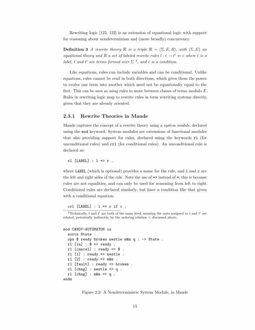
mod CANDY-AUTOMATON is
sorts State .
ops $ ready broken nestle m&m q : -> State .
rl [in] : $ => ready .
rl [cancel] : ready => $ .
rl [1] : ready => nestle .
rl [2] : ready => m&m .
rl [fault] : ready => broken .
rl [chng] : nestle => q .
rl [chng] : m&m => q .
endm
Figure 2.2: A Nondeterministic System Module, in Maude
15
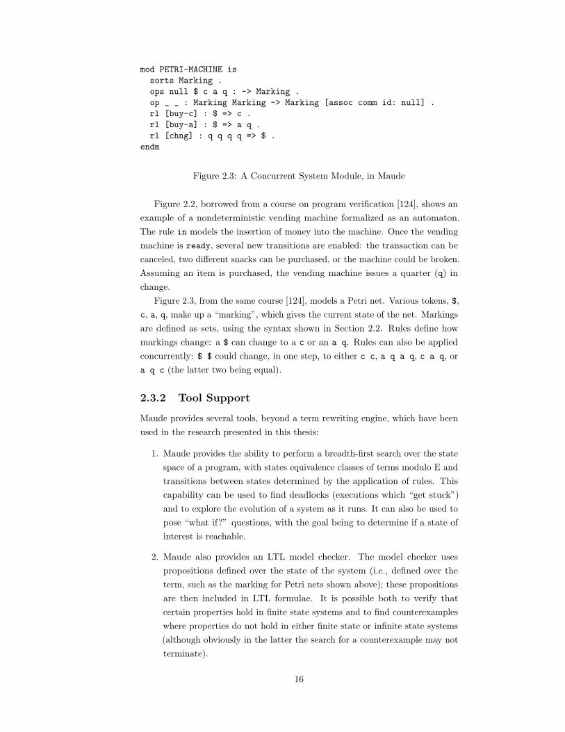
mod PETRI-MACHINE is
sorts Marking .
ops null $ c a q : -> Marking .
op _ _ : Marking Marking -> Marking [assoc comm id: null] .
rl [buy-c] : $ => c .
rl [buy-a] : $ => a q .
rl [chng] : q q q q => $ .
endm
Figure 2.3: A Concurrent System Module, in Maude
Figure 2.2, borrowed from a course on program verification [124], shows an
example of a nondeterministic vending machine formalized as an automaton.
The rule in models the insertion of money into the machine. Once the vending
machine is ready, several new transitions are enabled: the transaction can be
canceled, two different snacks can be purchased, or the machine could be broken.
Assuming an item is purchased, the vending machine issues a quarter (q) in
change.
Figure 2.3, from the same course [124], models a Petri net. Various tokens, $,
c, a, q, make up a “marking”, which gives the current state of the net. Markings
are defined as sets, using the syntax shown in Section 2.2. Rules define how
markings change: a $ can change to a c or an a q. Rules can also be applied
concurrently: $ $ could change, in one step, to either c c, a q a q, c a q, or
a q c (the latter two being equal).
2.3.2 Tool Support
Maude provides several tools, beyond a term rewriting engine, which have been
used in the research presented in this thesis:
1. Maude provides the ability to perform a breadth-first search over the state
space of a program, with states equivalence classes of terms modulo E and
transitions between states determined by the application of rules. This
capability can be used to find deadlocks (executions which “get stuck”)
and to explore the evolution of a system as it runs. It can also be used to
pose “what if?” questions, with the goal being to determine if a state of
interest is reachable.
2. Maude also provides an LTL model checker. The model checker uses
propositions defined over the state of the system (i.e., defined over the
term, such as the marking for Petri nets shown above); these propositions
are then included in LTL formulae. It is possible both to verify that
certain properties hold in finite state systems and to find counterexamples
where properties do not hold in either finite state or infinite state systems
(although obviously in the latter the search for a counterexample may not
terminate).
16

sorts Exp .
subsort Name < Exp .
op _; : Exp -> Stmt .
op Nil : -> Exp .
op if_then_else_fi : Exp Stmt Stmt -> Stmt .
op while_do_od : Exp Stmt -> Stmt .
Figure 2.4: RLS Abstract Syntax Definitions
2.4 Rewriting Logic Semantics
Equational logic has long been seen as a viable formalism for defining the
semantics of sequential programming languages [70, 68]. Rewriting logic extends
this by providing a formalism for defining the semantics of nondeterministic
and concurrent languages, leading to an area of research known as rewriting
logic semantics [128, 129]. One specific style of rewriting logic semantics, which
influenced the development of K (discussed in Section 2.5) and includes some of
the work discussed in this thesis, is computation-based rewriting logic semantics.
2.4.1 Computation-Based Rewriting Logic Semantics
The computation-based style of rewriting logic semantics (hereafter RLS) defines
the semantics of a programming language as a rewrite theory. The definition of
the semantics is given in an operational style, with terms used to represent the
current configuration – the current program and state – and rewriting logic rules
and equations used to represent transitions between configurations.
Sorts and Operations in RLS
The signature Σ contains sorts and operators representing: the abstract syntax
of the defined language; the configuration as a whole, as well as the various
parts that make up the configuration (e.g., an algebraic definition of the concept
of an environment); and the various auxiliary operations used as parts of the
semantics, including the individual operations used in the definitions of various
language features and the concept of a computed value. As a shorthand, this
last category is referred to later as semantic entities. Note that the distinction
between these three groups is arbitrary and made just to ease discussion: the
sort and operator syntax shown above for Maude is used to define all three.
Abstract Syntax: Examples of abstract syntax from the KOOL language,
discussed further in Chapter 3, are shown in Figure 2.4. First, a sorts declaration
defines a new sort, Exp, representing expressions in the abstract syntax for KOOL.
The subsort declaration specifies that terms of sort Name are also considered
to be of sort Exp, similar to a BNF production like Exp ::= Name . Several
operators then declare parts of the abstract syntax. The first, common in many
17

op empty : -> KState .
op _ _ : KState KState -> KState [assoc comm id: empty] .
op cset : ClassSet -> KState .
op env : Env -> KState .
op k : Computation -> KState .
op t : KState -> KState .
Figure 2.5: RLS Configuration Definitions
languages, says that an expression can also be used as a statement, indicated
by following it with a semicolon. The second defines the constant Nil, the null
reference value for KOOL. The third defines a standard conditional, with an
expression and two statements, one for each branch. The last defines a while loop,
again with a condition and then the loop body. Defining the abstract syntax
using mixfix notation provides a way to use notation which closely resembles
the actual language constructs and which can easily be mentally converted into
BNF – words in the operator are tokens, each underscore can be replaced by
the sort it represents to fill in the nonterminals, and the sort after the arrow
could be moved to the front before ::=. For instance, the operator declaration
while do od becomes Stmt ::= while Exp do Stmt od.
Configuration Items: Configuration items are also defined as operators,
and represent the same items used in other styles of semantics, such as environ-
ments, stores, and tables of information about functions, classes, methods, etc.
Configuration operators generally all have the same target sort, but can have
any argument sorts, holding individual pieces of information, arbitrary tuples,
lists, sets, finite maps, and multisets. Several sample configuration items from
KOOL, as well as the general declaration for configurations, are shown in Figure
2.5.
In Figure 2.5, all configuration items are given sort KState. KState itself
is defined as a multiset: putting together two KStates forms a new KState,
and during matching (i.e., when deciding which equations and rules to apply),
individual KState items can be rearranged (comm) and grouped (assoc) as
needed. This provides two advantages: configuration items do not need to be
named in a specific order in equations and rules; and items that are not needed
do not need to be included in the equation or rule, making the semantics more
modular (a point discussed further both in Section 2.5 and Chapter 9). Multisets
also allow the same configuration item to appear multiple times, which is useful
for items (such as threads) that can be repeated and which could (in theory)
have the same contents, but which should not be collapsed into the same item.
Four configuration items are then defined, cset, env, k, and t. cset holds a
set of classes, used in KOOL to keep track of classes that have been defined; env
holds the current environment, defined as a finite map, which maps the names of
18

variables to their locations in memory; and t is used to represent the state local
to an individual thread, defined as a multiset of other configuration items. This
provides a natural way to model the fact that some information is local to (and
present in) each thread, such as the current environment for a method running
in the thread, while some information is global to the entire computation, like
shared memory.
k holds the current computation, and deserves special mention since it is
a key part of the semantics. Computations in k are lists; each item in the list
is referred to as a computation item, each of which represents an individual
task or piece of information in the computation. The head of the list can be
seen as the “next” task, with the tail containing tasks that will be computed
later. Instead of using “,” as the list separator, an arrow, written in text as
-> and mathematically as y, is used instead, hopefully providing some added
intuition: do this (computation item ci1), then that (ci2), then that (ci3), etc,
until finished (cin is finished):
ci1 y ci2 y ci3 y ... y cin
The equations and rules used to define the semantics (discussed below) often
break up computations into smaller pieces, which are then put at the head of
the computation to indicate that they need to be computed first before the
overall computation can continue. Computations in RLS are just first-order
terms, making them easy to manipulate, for instance by saving the current
computation to resume later (for coroutines) or by creating a computation to
act as an exception handler.
The configuration item defined in Figure 2.5 are actually part of a much
larger configuration for KOOL, shown in Figure 2.6 and discussed further in
Chapter 3. Configurations in RLS are often hierarchical, with some parts of the
configuration (such as the current computation, the environment, etc) nested
inside other parts of the configuration (such as individual threads). As mentioned
above, this provides a natural way to duplicate parts of the configuration where
needed. It also provides a way to group related pieces of information and then
refer to them as a unit, instead of having to refer to each piece of information
individually.
Semantic Entities: Finally, semantic entities are defined similarly to abstract
syntax and configuration items. Figure 2.7 shows several examples: iv, which
“injects” integers into the sort Value, indicating that integers are valid values (i.e.,
results of computations) in KOOL; a definition of ObjEnv, or object environments,
used to track mappings from names to locations at each allocated “level” of
an object (this is covered in detail in Chapter 3); and release, a computation
item (as discussed in the context of the k cell above, and represented using sort
ComputationItem) defined as part of the semantics for concurrency in KOOL
19

Config
StringList
ControlEnvironment
StringList
Store
ClassSet
MethodStack ExceptionStack LoopStackComputation
Value Name
cset
mem
output
input
k mstack estacklstack
Nat
nextloc
Thread
env controlcobj
cclass
t*
LockSet
LockTupleSet
busy
holds
NameNat
lbl tid
Nat
nextTid
Threads
threads
Nat
Bool
tc
aflag
Figure 2.6: Concurrent KOOL State Infrastructure
that, when found in the current computation (in k), indicates that a lock is to
be released.
Equations and Rules in RLS
Using the signature discussed above, a number of equations and rules are
given to define the semantics of a language. In general, equations are used to
define deterministic features, with rules defining nondeterministic and concurrent
features.
Figure 2.8 shows several examples of equations used to define the semantics
of KOOL, along with the definitions of the auxiliary operations used in the
equations. The first provides the semantics for the statement E ; (the stmt
operation allows statements to be treated as part of the computation), saying that
this is defined as the result of evaluating the expression E and then discarding
the result. Note that exp(E) is placed “on top of” (i.e., to the left of) discard
in the computation, meaning that it will be evaluated first, with the expectation
that it will produce a value. The second equation provides a semantics for an
expression made up of just the name X: X is looked up to retrieve its current
op iv : Int -> Value .
op [_,_] : Name Env -> ObjEnv .
op release : -> ComputationItem .
Figure 2.7: RLS Semantic Entity Definitions
20

value. The third equation provides the semantics for assignment: when assigning
E to X, E is evaluated, and the resulting value is assigned to X using the assignTo
computation item.
One important point to note with these first three equations is that none
of them mention the k configuration item explicitly: these equations are valid
anywhere the underlying constructs are encountered (note that in the third
equation the semantics state that the value of E will be assigned to X, but the
assignment is done later, after E is evaluated). Other equations, which define
the semantics of constructs that depend on the current configuration, explicitly
mention k to ensure that they only apply when the defined construct is the next
task to evaluate in the computation. This can be seen in the fourth equation,
which defines the semantics of lookup. The environment, Env, is a finite map;
Env[X] is the lookup operation on the map, which should yield a location L in
the store where the value assigned to X is held. The condition does this lookup,
binding the location to L. This is represented using the := syntax, which binds
the term, here just a variable, on the left hand side to the result of reducing
the right hand side to a normal form, i.e., one where no rules or equations
can apply. The equation then checks to see if L is undefined, representing the
case when a name not in the environment is used. If the location is defined,
the value at the location is looked up in the store using the location lookup
(llookup) computation item. This equation should only apply when the lookup
is the next item in the computation to ensure that changes to the state are
properly sequenced, ensuring here that the environment used is the currently
active environment. One more point to note about this equation is the use
of CS, which represents the other contents of configuration item control, a
multiset of control-flow related items (the current computation, information
about exceptions and loops, etc). A way to eliminate the need to mention
op stmt : Stmt -> ComputationItem .
op exp : Exp -> ComputationItem .
op discard : -> ComputationItem .
op lookup : Name -> ComputationItem .
op assignTo : Name -> ComputationItem .
op llookup : Location -> ComputationItem .
eq stmt(E ;) = exp(E) -> discard .
eq exp(X) = lookup(X) .
eq stmt(X <- E ;) = exp(E) -> assignTo(X) .
ceq control(k(lookup(X) -> K) CS) env(Env) =
control(k(llookup(L) -> K) CS) env(Env)
if L := Env[X] /\ L =/= undefined .
Figure 2.8: RLS Semantics with Equations
21

rl threads(t(control(k(stmt(label(X)) -> K) CS) lbl(X’) TS) KS)
=> threads(t(control(k(K) CS) lbl(X) TS) KS) .
crl threads(t(control(k(val(V) -> acquire -> K) CS)
holds(LTS) TS) KS) busy(LS)
=> threads(t(control(k(K) CS)
holds(LTS [lk(V),1]) TS) KS) busy(LS lk(V))
if notin(LS,lk(V)) .
Figure 2.9: RLS Semantics with Rules
such “unused” parts of the configuration added only for matching is part of K,
discussed in Section 2.5.
Figure 2.9 shows the semantics of two concurrency-related features, defined
using rules. The first rule, which is not conditional, defines the semantics of
label statements, which provide a way for the user to give labels in program code
that can then be used when model checking programs. When a label statement
with label X is the next item in the computation, the label associated with the
current thread is changed from X’ (the former value) to X. Here CS, TS, and KS
are all used to represent unreferenced parts of the configuration. Configuration
item t is a multiset with information for one thread, while threads is a multiset
containing all the threads active in a program.
The second rule, which is conditional, defines the semantics for lock acqui-
sition, given in K syntax in Chapter 3, Rule 3.33. Like Java, KOOL acquires
locks on specific values. Here, a lock is being acquired on a value V. The locks
the thread currently holds are in the holds item (LTS), while the locks held
by all threads are part of the busy item (LS). If the lock is not in LS (meaning
it is not held by another thread), it can be acquired, which results in it being
added both to the busy item and to the thread-local holds item. When added
to holds a lock count is also maintained, which is used to model cases where
the same thread acquires multiple locks on the same value, ensuring that the
locked value is released the proper number of times before it is removed from
busy and can be acquired by another thread.
2.5 K
K [167], based on rewriting logic and the work on the computation-based style of
rewriting logic semantics discussed above, is a general technique and notation for
defining deterministic, nondeterministic, and concurrent computation. In this
thesis, the focus is specifically on formal definitions of programming languages,
which was the first application of K. Beyond the prior work on rewriting logic
semantics, K was also influenced by work on abstract state machines (ASMs)
[74], the chemical abstract machine (CHAM) [64], and continuations [184]. K
takes its name from k, the name of the configuration item used to hold the
22

current computation. While there are many similarities between K and the
computation-based style of rewriting logic semantics, there are some significant
differences as well, mainly in providing additional support for modularity and
for writing concise language definitions.
2.5.1 K Configurations
Configurations in K are defined identically to how they are defined using RLS.
In K, each configuration item is referred to as a K cell. The current computation
is still stored inside a k configuration item, or k cell, and it is still possible (as in
the case of threads) to have multiple copies of all cells, including k, if needed
by the semantics. A second standard cell, ⊤, represents the entire configuration
(i.e., the entire term).
2.5.2 K Sorts and Operations
Signatures in K are identical to signatures in RLS with one exception: several
new attributes for operations have been added, used by K to automatically
handle some routine language definition tasks.
The most common of these is strict, which is used on operator definitions
to indicate that the operands must be evaluated first before evaluating the entire
operation. This was done manually before in RLS, leading to a large number of
equations and operators used just to indicate how operands were being evaluated.
A common case is with arithmetic operations, such as addition, where the RLS
definition would be:
op _+_ : Exp Exp -> Exp .
op plus : -> ComputationItem .
eq exp(E + E’) = exp(E,E’) -> plus .
eq val(iv(I),iv(I’)) -> plus -> K = val(iv(I + I’)) -> K .
Here, two operators had to be defined. The first is the abstract syntax for
plus, which would be needed regardless; the second is a placeholder computation
item, added into the computation to indicate that the computation is “waiting”
for the two operands to be evaluated before evaluating the plus. The actual
equations are then shown. The first says that, to evaluate E + E’, one must first
evaluate E and E’, again using the plus computation item to indicate that an
addition will occur once E and E’ are evaluated. The second equation applies
after E and E’ have been evaluated to two integer values, I and I’. In this case,
the value returned is the sum of I and I’.
In K, this can be indicated as:
op _+_ : Exp Exp -> Exp [strict] .
iv(I) + iv(I’) => iv(I + I’) .
23

Behind the scenes, K will generate the intermediate operators to evaluate E
and E’ automatically, putting the values back into the positions of the original
operands. This allows the semantic equation to use a form closer to the original
syntax, instead of having the result values on top of an intermediate computation
item in the computation. In cases where not every argument position should
be strict, a list of natural numbers, indicating the strict positions, can also be
provided. This is the case with a conditional, for instance, where one should
evaluate the condition before choosing which branch is evaluated. For cases
where the evaluation order is important, a variant of strict, seqstrict, can
be used instead, which will enforce a left to right order of evaluation on all strict
argument positions. Finally, note that the semantics given above use a rule
(indicated as in rewriting logic with =>), not an equation as may be expected;
the reason for this is explained next.
2.5.3 K Rules and Equations
A K definition consists of two types of sentences: structural equations and rewrite
rules. Structural equations carry no computational meaning, and, like equational
logic equations, can be used for reasoning both from left to right and from right
to left. When converted into term rewrite rules they are treated the same as
equations in equational logic, evaluating from left to right. One use of structural
equations is to provide definitions for auxiliary operations used in the semantics.
Examples include operations to work with the lists and sets (list length, set
membership, etc) included in the configuration, or operations to pull apart the
abstract syntax to get useful information (the type of a declaration, the number
of pointer “levels” in a C pointer declaration, the branches of a conditional, etc).
Equations used to desugar language syntax are also considered to be structural,
and include transformations such as turning a one-armed conditional into a
two-armed conditional with a default else body.
One special type of structural equation, used with the strict and seqstrict
attributes discussed above, is a heating/cooling rule. In the Chemical Abstract
Machine, computations are represented as molecular soups, with information
stored inside individual molecules. To allow computation, the information inside
each molecule needs to move outside the molecule membrane, where it can
encounter other information and interact. This process is called heating, and in
K is represented by placing operands on top of the computation. In the Chemical
Abstract Machine, the computation then cools, with the new compounds (i.e.,
the results of the computation) going back into molecules where they can no
longer directly interact. The K equivalent is when the computed values are
placed back into the original abstract syntax item, like iv(I) + iv(I’) above.
While it is not necessary to write these rules by hand – one can assume that
they are automatically created by the use of strictness attributes – it is possible
to do so. When written manually, they are given a special notation using the ⇋
24

symbol to separate the two sides of the equation. This is solely to provide added
intuition, and could be represented using two equations instead, one using the
unevaluated form (like a1) and one using the evaluated form (like i1). Examples
of heating and cooling rules include:
a1 + a2 ⇋ a1 y � + a2 (2.2)
i1 + a2 ⇋ a2 y i1 + � (2.3)
if b then s1 else s2 ⇋ b y if � then s1 else s2 (2.4)
K automatically generates special operators, serving the same purpose as the
plus computation item defined manually above, to represent the intermediate
steps being taken in the computation. When an operand is placed on top of the
computation through heating, the operand position is replaced with a �, leading
to operators like � + in equation 2.2, + � in equation 2.3, and if � then else
in equation 2.4. The cooled value would then go back into the position of the
box. Note that the equations in 2.2 and 2.3 show the deterministic version
(seqstrict), since the first operand must evaluate to a value before the second
is evaluated.
Unlike structural equations, rewrite rules represent actual steps of computa-
tion. Examples include:
i1 + i2 → i, where i is the sum of i1 and i2 (2.5)
if true then s1 else s2 → s1 (2.6)
if false then s1 else s2 → s2 (2.7)
Rule 2.5 is the standard addition rule, taking i1 + i2 to the sum of i1 and i2.
Like rules in rewriting logic, K rules represent a one-way transition, allowing
reasoning from left to right only. Rules 2.6 and 2.7 provide the semantics for
the if statement, with the correct path chosen based on whether the condition
evaluates to true or false.
Up to now, the rules have not referenced K cells. The cells are given in K
rules using an XML-like notation, with an opening cell “tag”, like 〈k〉 and a
closing tag like 〈/k〉. The last rule, rule 2.8, shows an example using multiple
cells with this XML-like notation. This is a variant of the KOOL assignment
rule, with variable X being assigned value V . The environment (env) and store
(mem) cells both hold finite maps, represented as a set of pairs, with operations
defined for both to ensure the uniqueness of the first projection of each pair.
As in Figure 2.9, TS and CS are used to match other parts of the thread and
25

control states:
〈t〉 〈control〉 〈k〉 X ← V y K 〈/k〉 CS 〈/control〉 〈env〉 (X, L) Env 〈/env〉 TS 〈/t〉
〈mem〉 (L, V ′) Mem 〈/mem〉 →
〈t〉 〈control〉 〈k〉 K 〈/k〉 CS 〈/control〉 〈env〉 (X, L) Env 〈/env〉 TS 〈/t〉
〈mem〉 (L, V ) Mem 〈/mem〉 (2.8)
At this point, Rule 2.8 looks like an RLS rule, but with the cells given in
an XML-like notation instead of prefix notation. K includes special notation to
help simplify rules and make them more modular. The most important is that
context needed only for matching the configuration structure, including variables
such as CS and TS and cells such as t and control , can be elided:
〈k〉 X ← V y K 〈/k〉 〈env〉 (X,L) Env 〈/env〉
〈mem〉 (L, V ′) Mem 〈/mem〉 →
〈k〉 K 〈/k〉 〈env〉 (X,L) Env 〈/env〉
〈mem〉 (L, V ) Mem 〈/mem〉 (2.9)
This is not just a notational convenience: requiring this extra context makes
the rules less modular, since changes to the layout of the configuration (adding a
new level, moving cells between levels) would require changes to the rule. Since
this information is still needed for matching, it is added back in using context
transformers, which will transform each rule into a rule with a complete matching
context, based on the structure of the configuration. Context transformers are
discussed further below.
Another feature, which is just a notational convenience, is the ability to
replace variables that are given on the left-hand side of a rule but are not
otherwise used (in conditions or on the right-hand side) with an underscore,
similar to functional languages such as OCaml [163, 4]. This is used below to
replace V ′, given in Rule 2.9, with an underscore, since it is not used elsewhere
in the rule:
〈k〉 X ← V y K 〈/k〉 〈env〉 (X,L) Env 〈/env〉
〈mem〉 (L, ) Mem 〈/mem〉 →
〈k〉 K 〈/k〉 〈env〉 (X,L) Env 〈/env〉
〈mem〉 (L, V ) Mem 〈/mem〉 (2.10)
Since matching against lists and sets is used quite often, it is also helpful to
have special notation for both lists and sets. In K, this is indicated by using
“...”, with a “...” at the start or end of a cell indicating a list match (“...” at the
start would indicate that one is matching the tail of the list, while “...” at the
26

end would indicate that one is matching the head), and “...” at both ends of the
cell indicating a set or multiset match5. Rule 2.10 can be transformed to use
this notation, with the result given below in Rule 2.11:
〈k〉 X ← V ...〈/k〉 〈env〉... (X, L) ...〈/env〉
〈mem〉... (L, ) ...〈/mem〉 →
〈k〉 · ...〈/k〉 〈env〉... (X, L) ...〈/env〉
〈mem〉... (L, V ) ...〈/mem〉 (2.11)
In Rule 2.11, the “...” convention allows us to just mention the pair being
used in the environment and store, while eliding the rest of the cell contents. k
is a list, so the convention indicates that we are just matching the head. Since
we are eliminating the head element, and not replacing it with anything else, we
indicate this with ·.
Finally, some of the information in Rule 2.11 is redundant. For instance, the
environment does not change, but must be mentioned on each side of the rule,
since mentioning it just on the left-hand side would be the same as discarding
it. K provides a way to indicate that only certain parts of a term are changed
by a rule to reduce this redundancy. To do this, in the K notation it is possible
to underline the parts of a term that change, and then note the change (i.e.,
the right-hand side) underneath the line (i.e., under the left-hand side). The
arrow between the two sides (→) is also dropped, since it is no longer needed; to
reconstruct the right-hand side of the rule, the “top” of the K rule can be copied
to the right-hand side, with any underlined portions replaced by the subterms
given below the line.
〈k〉 X ← V
·
...〈/k〉 〈env〉... (X, L) ...〈/env〉 〈mem〉... (L,
V
) ...〈/mem〉
(2.12)
Rule 2.12 shows an example where this has been done. In the k cell, the · is
now under X := V , while V is now under . Since both the environment and
the first element (L) of the pair in mem do not change, each only needs to be
written once.
2.5.4 Rules and Equations in K and RLS
The use of rules and equations is slightly different in K and RLS. In RLS, equa-
tions are used to represent deterministic language features, while rules represent
language features that can be affected by nondeterminism and concurrency,
5This is purely a notational convention, to indicate that the match is being performedmodulo both associativity and commutativity; it would be possible to change the notation tojust use one “...”, but this would make the type of match less obvious in the rule.
27
such as memory reads and writes that could lead to data races, or attempts
to acquire locks. Some recent work [129] has instead looked at the use of rules
and equations in terms of computational abstraction, with the ability to move
from a specification with all equations to one with all rules seen as turning
an “abstraction knob” from a more abstract (all equations) to less abstract (all
rules) definition. This allows the language designer to capture the idea of a
computational step more closely, with each rule representing a discreet step (like
a transition in a structural operational semantics definition).
This latter view is the perspective taken in K. Computational steps are
defined as rewrite rules, while other parts of the computation are defined using
structural equations, with the ability to “tune” this based on what should be
considered a step of computation. In mapping K to Maude, structural equations
and rules can be mapped directly to Maude equations and rules, although this
mapping will often be modified based on the planned use of the semantics. For
instance, for model checking, most K rules will be mapped to equations, with
only those rules directly interacting with concurrency mapped to Maude rules.
2.5.5 Context Transformers
To ensure that rules are modular, it should be possible to continue using a rule,
unchanged, when parts of the context (i.e., K cells) not mentioned in the rule
are modified or replaced. Given a specific rule, the easiest case to deal with
is when the part of the configuration matched by a rule remains the same but
the surrounding context changes. This case is handled naturally in both RLS
and K by defining the configuration as an associative, commutative multiset of
configuration items (often referred to a a “soup”). Because the configuration is
commutative, the ordering of the individual items does not matter, meaning it is
not essential to put items in positions and then name them even when not used,
as it would be if the configuration were represented as a tuple. Associativity then
allows arbitrary groupings of items, meaning we don’t have to worry about the
order in which the set is formed (i.e., there is no difference between set 1 (2 3)
and set (1 2) 3, both can just be treated as 1 2 3).
The more challenging case is when the configuration used by a rule is changed.
A common example is when new levels are added to the cell hierarchy. For
instance, when threads are added to a language, thread-specific information is
grouped into a thread cell, often called t, while information that is global to the
computation is left at its current level. Rules that referenced both information
that is now inside the thread cell and global information would then need to
be changed to account for this added level of nesting. An example is Rule 2.8,
the assignment rule, which used the computation (k), environment (env), and
store (mem) cells. When threads are added, the computation and environment
are grouped inside t, but the store is not, since there is only one which is shared
by all threads. In RLS this leads to a revision of the assignment rule, shown
28

below in Rule 2.13.
〈t〉... 〈k〉X := V
·
...〈/k〉 〈env〉... (X, L) ...〈/env〉 ...〈/t〉 〈mem〉... (L,
V
) ...〈/mem〉 (2.13)
Rule 2.13 shows the type of change typically made within a language, but
it is also important that language features, once specified, can be used across
languages, providing a method to build languages more quickly by assembling
them from trusted pieces. This provides an additional challenge, since the
configuration in a different language may be quite different from that used in
the language where the feature was originally defined. In this case, using RLS
rules would often need to be manually changed from one language to another to
accommodate differences in configurations. K solves this problem through the
use of context transformers:
Definition 4 A context transformer, t, is a function which takes as input a K
configuration k and a K sentence (i.e., a K rule or equation) s and generates a
new sentence, s′. For any two cells c and c′ in s, s′ is created by t to include
any cells cn which occur between c and c′ in k. This process, context completion,
allows a correct match against the configuration structure k using s′. In cases
where t is unable to calculate a unique completion for s′, s is said to be ambiguous.
Context completion works using a combination of the information given in
the configuration (such as indications that cells can be repeated), information in
s (any already specified context), and various rules and heuristics (such as using
the shortest path in k between c and c′). Since in general there are many possible
completions, the rules and heuristics are needed to identify a single completion,
which should be the intended completion (i.e., the completion containing the
context that would otherwise have been written by hand). If s is ambiguous, this
means that there are multiple possible completions that comport with the given
rules and heuristics, so additional context information must be added manually
to s before s′ can be generated by t.
Using context transformers, only those portions of the configuration actually
used in a rule need to be mentioned, with other parts of the configuration, needed
only to ensure a valid match, added automatically. For instance, the assignment
rule shown originally in Rule 2.8 can remain as is, without the need to explicitly
add the thread cell as was done for Rule 2.12. This accommodates changes
within a language and changes between languages, under the assumption that
the cell names themselves do not change.
2.5.6 K Notation Changes
Since it was first introduced [86, 32] the K notation has gone through several
iterations, mainly involved with how the cells are represented. At first, K cells
were represented using standard Maude notation – the computation cell would
29

be represented as k(K), with K being the actual computation inside the cell.
This later changed to allow for specific notation for lists and sets inside cells,
replacing the standard opening or closing parentheses with a (left or right)
angle to represent that more information was included “in that direction”,
represented now using “...”. For instance, to match the first element in the
computation, the notation would use k(item >, adapted later to k(| item |>.
A more mathematical notation was then adopted, with the cell label added as
a subscript to the cell, like Litem|〉k [167]. Based on feedback from others, the
current notation uses the XML-like notation presented in this thesis. An attempt
has been made to ensure all semantic rules presented in this thesis that are
written in K, and not Maude, syntax make use of this current notation, but this
change needs to be kept in mind when referencing earlier work.
30

Chapter 3
Language Prototyping
Language design is much more an art than a science. Selecting from the
wide range of available language features, designing new features, and choosing
appropriate syntax are all important tasks which do not have clear ”best” answers.
Sometimes even small decisions in any of these areas can drastically impact the
usability, or feel, of a language.
One method to improve the language design process is language prototyping.
Prototypes provide the same advantages for designing languages as they provide
for designing programs: by actually using the language features being designed,
instead of just seeing them on paper, the designer can gain confidence that
the features work well, or discover early in the process that they do not. Also,
definitions of features in a prototype must include enough detail to allow them
to be used with programs, highlighting areas of the design that appear complete
on paper but are unclear in practice. The ability to use the prototyped features
also provides opportunities to see how different features of the same language
interact, helping to prevent poor feature interactions from making it into a
settled version of the language. Having a method for prototyping languages
that does not require the time and effort involved in modifying a compiler or
interpreter provides additional benefits, allowing the design process to proceed
more rapidly.
Ideally, language prototypes will be formal, providing a clearer definition of
the features being designed than is possible with normal textual descriptions,
such as those found in manuals. Having a formal definition also opens the
process up to the use of formal tools, such as model checkers, state space search
tools, and theorem provers. These not only allow proofs about programs and
properties of the language (the latter referred to as language meta-theory proofs),
but can also provide ways to gain confidence that a language is working as
expected. For instance, using state space search techniques, it may be possible
to show that only expected states can be reached in certain sample programs
when using certain concurrency features in a language. This type of tool support
is especially important with the addition of complex abstraction capabilities
and new concurrency features, both of which make programs and programming
languages more challenging to understand.
The remainder of this chapter illustrates language prototyping using a case
31
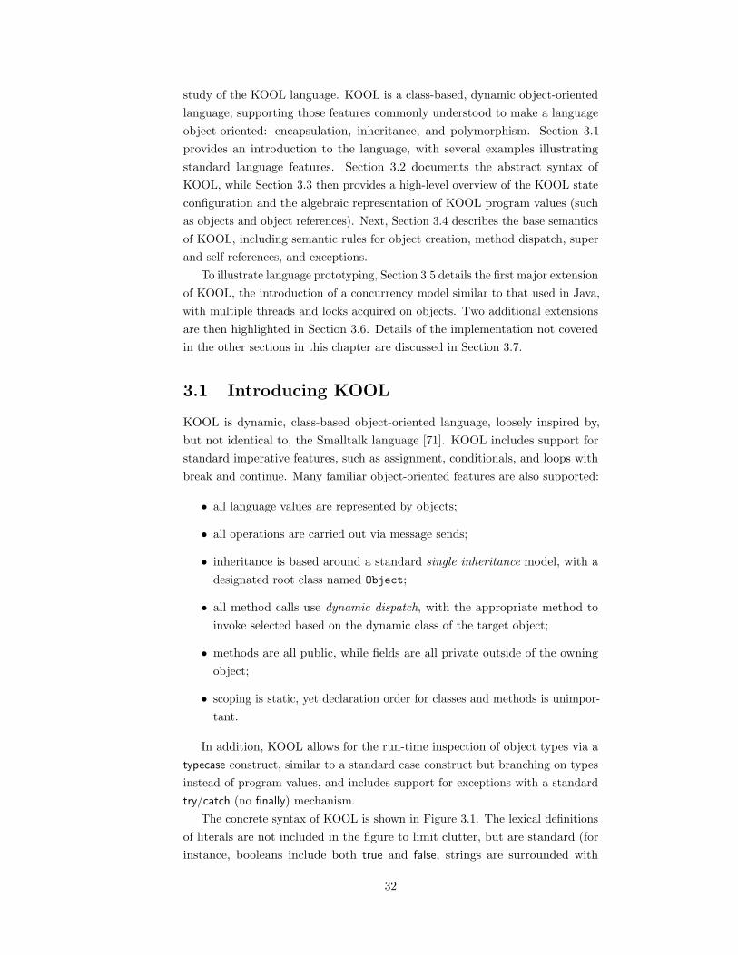
study of the KOOL language. KOOL is a class-based, dynamic object-oriented
language, supporting those features commonly understood to make a language
object-oriented: encapsulation, inheritance, and polymorphism. Section 3.1
provides an introduction to the language, with several examples illustrating
standard language features. Section 3.2 documents the abstract syntax of
KOOL, while Section 3.3 then provides a high-level overview of the KOOL state
configuration and the algebraic representation of KOOL program values (such
as objects and object references). Next, Section 3.4 describes the base semantics
of KOOL, including semantic rules for object creation, method dispatch, super
and self references, and exceptions.
To illustrate language prototyping, Section 3.5 details the first major extension
of KOOL, the introduction of a concurrency model similar to that used in Java,
with multiple threads and locks acquired on objects. Two additional extensions
are then highlighted in Section 3.6. Details of the implementation not covered
in the other sections in this chapter are discussed in Section 3.7.
3.1 Introducing KOOL
KOOL is dynamic, class-based object-oriented language, loosely inspired by,
but not identical to, the Smalltalk language [71]. KOOL includes support for
standard imperative features, such as assignment, conditionals, and loops with
break and continue. Many familiar object-oriented features are also supported:
• all language values are represented by objects;
• all operations are carried out via message sends;
• inheritance is based around a standard single inheritance model, with a
designated root class named Object;
• all method calls use dynamic dispatch, with the appropriate method to
invoke selected based on the dynamic class of the target object;
• methods are all public, while fields are all private outside of the owning
object;
• scoping is static, yet declaration order for classes and methods is unimpor-
tant.
In addition, KOOL allows for the run-time inspection of object types via a
typecase construct, similar to a standard case construct but branching on types
instead of program values, and includes support for exceptions with a standard
try/catch (no finally) mechanism.
The concrete syntax of KOOL is shown in Figure 3.1. The lexical definitions
of literals are not included in the figure to limit clutter, but are standard (for
instance, booleans include both true and false, strings are surrounded with
32

Program P ::= C∗
E
Class C ::= class X is D∗
M∗
end | class X extends X′
is D∗
M∗
end
Decl D ::= var {X,}+
;
Method M ::= method X is D∗
S end | method X ({X′
,}+
) is D∗
S end
Expression E ::= X | I | F | B | Ch | Str | (E) | new X | new X ({E,}+
) |
self | E Xop E′
| E.X(())?| E.X({E,}
+) | super() |
super.X(())?| super.X({E,}
+) | super({E,}
+) | primInvoke({E,}
+)
Statement S ::= E <- E′
; | begin D∗
S end | if E then S (else S′
)?
fi |
try S catch X S end | throw E ; | while E do S od |
for X <- E to E′
do S od | break; | continue; |
return (E)?; | S S
′
| E; | typecase E of Cs+
(else S)?
end
Case Cs ::= case X of S
X ∈ Name, I ∈ Integer, F ∈ Float, B ∈ Boolean, Ch ∈ Char, Str ∈ String,
Xop ∈ Operator Names
Figure 3.1: KOOL Syntax
double quotes, etc). Most message sends are specified in a Java-like syntax;
those representing binary operations can also be used infix (a + b desugars to
a.+(b)), with these infix usages all having the same precedence and associativity.
Finally, semicolons are used as statement terminators, not separators, and are
only needed where the end of a statement may be ambiguous – at the end of
an assignment, for instance, or at the end of each statement inside a branch of
a conditional, but not at the end of the conditional itself, which ends with fi.
One important point is that many standard expressions are not defined as part
of the KOOL syntax, but instead are handled using message sends, such as the
arithmetic, logical, and boolean operations commonly found in programming
languages.
Figure 3.2 shows an example of the typical “Hello World!” program in KOOL.
A program in KOOL is made up of any (0 or more) user defined classes, followed
by an arbitrary KOOL expression, which has access to these classes as well as
classes provided in a standard KOOL prelude. console is a predefined object,
representing the standard input and output streams, with methods to read from
(>>) and write to (<<) the stream1. "Hello World!" is a string, which is actually
an object of class String. When << is invoked with an argument, it will call that
object’s toString method and then return itself, allowing multiple calls to <<
to be chained (such as console << "Value = " << 3). Since calling toString
on a string will just return the string value, this program just writes "Hello
World!" to standard output.
Figure 3.3 shows a slightly more complex example. Here, a new class
Factorial is defined with a method Fact that calculates the factorial of the
1These method names were borrowed from C++.
33
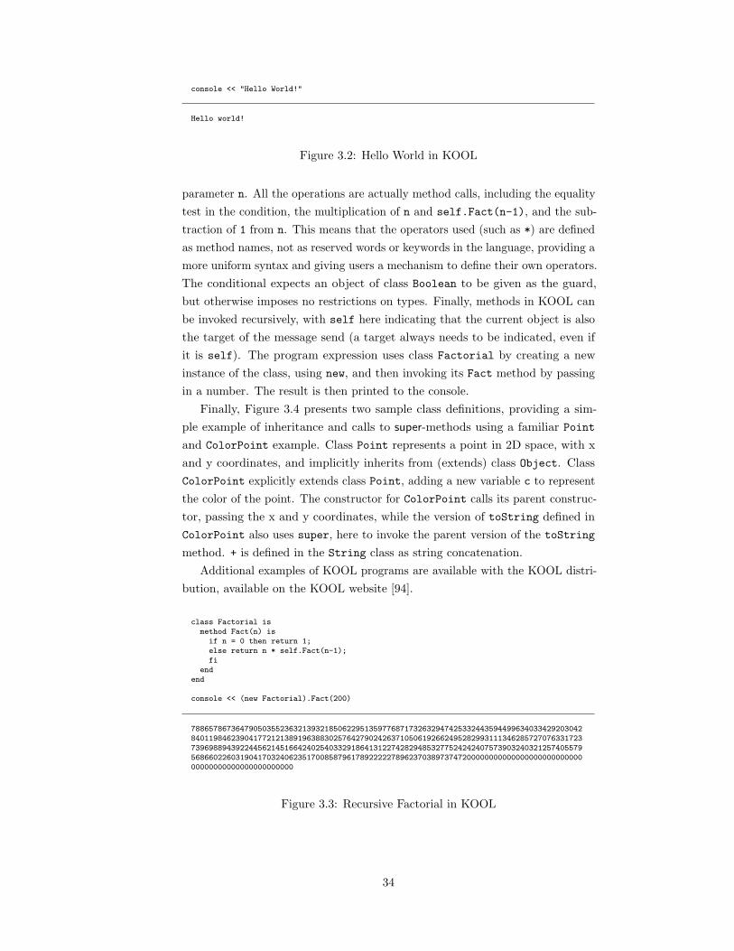
console << "Hello World!"
Hello world!
Figure 3.2: Hello World in KOOL
parameter n. All the operations are actually method calls, including the equality
test in the condition, the multiplication of n and self.Fact(n-1), and the sub-
traction of 1 from n. This means that the operators used (such as *) are defined
as method names, not as reserved words or keywords in the language, providing a
more uniform syntax and giving users a mechanism to define their own operators.
The conditional expects an object of class Boolean to be given as the guard,
but otherwise imposes no restrictions on types. Finally, methods in KOOL can
be invoked recursively, with self here indicating that the current object is also
the target of the message send (a target always needs to be indicated, even if
it is self). The program expression uses class Factorial by creating a new
instance of the class, using new, and then invoking its Fact method by passing
in a number. The result is then printed to the console.
Finally, Figure 3.4 presents two sample class definitions, providing a sim-
ple example of inheritance and calls to super-methods using a familiar Point
and ColorPoint example. Class Point represents a point in 2D space, with x
and y coordinates, and implicitly inherits from (extends) class Object. Class
ColorPoint explicitly extends class Point, adding a new variable c to represent
the color of the point. The constructor for ColorPoint calls its parent construc-
tor, passing the x and y coordinates, while the version of toString defined in
ColorPoint also uses super, here to invoke the parent version of the toString
method. + is defined in the String class as string concatenation.
Additional examples of KOOL programs are available with the KOOL distri-
bution, available on the KOOL website [94].
class Factorial ismethod Fact(n) is
if n = 0 then return 1;else return n * self.Fact(n-1);fi
endend
console << (new Factorial).Fact(200)
788657867364790503552363213932185062295135977687173263294742533244359449963403342920304284011984623904177212138919638830257642790242637105061926624952829931113462857270763317237396988943922445621451664240254033291864131227428294853277524242407573903240321257405579568660226031904170324062351700858796178922222789623703897374720000000000000000000000000000000000000000000000000
Figure 3.3: Recursive Factorial in KOOL
34

class Point isvar x,y;
method Point(inx, iny) isx <- inx;y <- iny;
end
method toString isreturn ("x = " + x.toString() + " and y = "
+ y.toString());end
end
class ColorPoint extends Point isvar c;
method ColorPoint(inx, iny, inc) issuper(inx,iny);c <- inc;
end
method toString isreturn (super.toString() + " and c = " + c.toString());
end
method write isconsole << self;
endend
(new ColorPoint(20,30,5)).write
x = 20 and y = 30 and c = 5
Figure 3.4: Inheritance and Built-ins in KOOL
3.2 Abstract Syntax
The abstract syntax of KOOL closely mirrors the concrete syntax, but in general
does not require as many cases, since in some cases several productions in the
concrete rules can be mapped to a single abstract syntax production. For instance,
binary infix operators are mapped to standard “dot-notation” message sends.
The definitions of abstract syntax shown below are provided using standard
Maude notation.
Names: The abstract syntax for names in KOOL takes advantage of the
Maude QID module, providing a way to represent arbitrary identifier strings
as quoted (i.e., preceded by a single quote, such as ’Boolean) strings in the
semantics. These quoted strings are wrapped in a special operator n, injecting
them into the Name sort. Lists of names, needed for parameter lists in method
definitions and in variable declarations, are also provided, with names in the list
separated by commas.
fmod NAME-SYNTAX is
protecting QID .
sort Name NameList .
subsort Name < NameList .
35

op n : Qid -> Name .
op empty : -> NameList .
op _,_ : NameList NameList -> NameList [assoc id: empty] .
endfm
Scalars: Scalars to represent integers, floating-point numbers, booleans, and
individual characters are also provided in the KOOL abstract syntax. Each
scalar is provided with a K-specific sort (e.g., KInt) into which it is injected.
The underlying representations are those offered by Maude. Strings are not
strictly scalars, but are literals, and so are included here as well for convenience.
fmod SCALARS-SYNTAX is
including INT .
including FLOAT .
including BOOL .
including STRING .
sorts KInt KFloat KBool KChar KString .
op i : Int -> KInt .
op f : Float -> KFloat .
op b : Bool -> KBool .
op c : Char -> KChar .
op s : String -> KString .
endfm
Expressions: Expressions in KOOL include (through subsorting) the prior
definitions of names and scalars. The abstract syntax for expressions also adds
expression lists, used in method calls, and a special expression, Nil, which
represents an object reference assigned to no object.
fmod EXP-SYNTAX is
including NAME-SYNTAX .
including SCALARS-SYNTAX .
sorts Exp ExpList .
subsort Exp < ExpList .
subsort Name KInt KFloat KBool KChar KString < Exp .
subsort NameList < ExpList .
op empty : -> ExpList .
op _,_ : ExpList ExpList -> ExpList [assoc id: empty] .
op Nil : -> Exp .
endfm
Statements: The base sort for statements in KOOL is Stmt. An expression
can be used as a statement by terminating it with a semicolon, represented with
the ; operator definition. A skip; statement is also introduced, representing a
statement that does nothing.
36
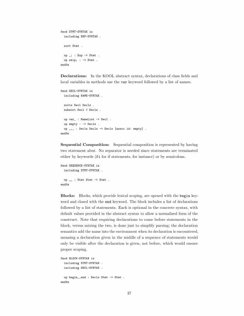
fmod STMT-SYNTAX is
including EXP-SYNTAX .
sort Stmt .
op _; : Exp -> Stmt .
op skip; : -> Stmt .
endfm
Declarations: In the KOOL abstract syntax, declarations of class fields and
local variables in methods use the var keyword followed by a list of names.
fmod DECL-SYNTAX is
including NAME-SYNTAX .
sorts Decl Decls .
subsort Decl < Decls .
op var_ : NameList -> Decl .
op empty : -> Decls .
op _,_ : Decls Decls -> Decls [assoc id: empty] .
endfm
Sequential Composition: Sequential composition is represented by having
two statement abut. No separator is needed since statements are terminated
either by keywords (fi for if statements, for instance) or by semicolons.
fmod SEQUENCE-SYNTAX is
including STMT-SYNTAX .
op __ : Stmt Stmt -> Stmt .
endfm
Blocks: Blocks, which provide lexical scoping, are opened with the begin key-
word and closed with the end keyword. The block includes a list of declarations
followed by a list of statements. Each is optional in the concrete syntax, with
default values provided in the abstract syntax to allow a normalized form of the
construct. Note that requiring declarations to come before statements in the
block, versus mixing the two, is done just to simplify parsing; the declaration
semantics add the name into the environment when its declaration is encountered,
meaning a declaration given in the middle of a sequence of statements would
only be visible after the declaration is given, not before, which would ensure
proper scoping.
fmod BLOCK-SYNTAX is
including STMT-SYNTAX .
including DECL-SYNTAX .
op begin__end : Decls Stmt -> Stmt .
endfm
37
Assignments: Assignment uses <- notation, with the value on the right and
the target on the left.
fmod ASSIGNMENT-SYNTAX is
including EXP-SYNTAX .
including STMT-SYNTAX .
op _<-_; : Exp Exp -> Stmt .
endfm
Conditionals: Conditionals, with and without else branches, are supported in
the abstract syntax. Only one is used in the semantics: a conditional without an
else clause is transformed into a conditional with an else skip; clause. Note
that this could also be done on the translation from concrete to abstract syntax.
fmod CONDITIONAL-SYNTAX is
including EXP-SYNTAX .
including STMT-SYNTAX .
op if_then_else_fi : Exp Stmt Stmt -> Stmt .
op if_then_fi : Exp Stmt -> Stmt .
endfm
Loops: for, while, and do/while loops are all supported in KOOL. KOOL
also allows break and continue statements, which either exit or restart (in the
case of the for loop, after incrementing the loop counter) the current loop.
fmod LOOP-SYNTAX is
including EXP-SYNTAX .
including STMT-SYNTAX .
including NAME-SYNTAX .
op for_<-_to_do_od : Name Exp Exp Stmt -> Stmt .
op while_do_od : Exp Stmt -> Stmt .
op do_while_od : Stmt Exp -> Stmt .
op break‘; : -> Stmt .
op continue‘; : -> Stmt .
endfm
Methods: A method in KOOL uses the method keyword, followed by the
method name, and then a list of method parameters. The method body is
bracketed with is and end, and includes a list of local declarations (optional
in the concrete syntax) and the method statement. The abstract syntax treats
multiple methods as a list, but these are converted into a method set in the
internal representation, since the order of declaration does not matter. Defined
with the method syntax is the abstract syntax for return. A return statement
without an expression is equivalent to returning the nil value.
fmod METHOD-SYNTAX is
including NAME-SYNTAX .
38

including DECL-SYNTAX .
including STMT-SYNTAX .
sorts Method MethodList .
subsort Method < MethodList .
op empty : -> MethodList .
op _,_ : MethodList MethodList -> MethodList [assoc id: empty] .
op method_‘(_‘)is__end : Name NameList Decls Stmt -> Method .
op return‘; : -> Stmt .
op return_; : Exp -> Stmt .
endfm
Classes: Classes in KOOL are given a class name, the name of the extended
class (this is not required in the concrete syntax, but is automatically added in
the abstract syntax – all classes that do not explicitly extend another class extend
Object), declarations of class fields, and a list of class methods. primclass is
used to identify that a class is used to model a primitive value in the language,
which enables support for manipulating this primitive value using the KOOL
primitives functionality.
fmod CLASS-SYNTAX is
including DECL-SYNTAX .
including NAME-SYNTAX .
including METHOD-SYNTAX .
sorts Class Classes .
subsort Class < Classes .
op _,_ : Classes Classes -> Classes [assoc id: empty] .
op empty : -> Classes .
op class_extends_is__end : Name Name Decls MethodList -> Class .
op primclass_extends_is__end : Name Name Decls MethodList -> Class .
endfm
Self: The self keyword represents the current object. It can be used wherever
a reference to the current object is needed, and also must be used when making
method calls where the current object is also the target.
fmod SELF-SYNTAX is
including NAME-SYNTAX .
including EXP-SYNTAX .
op self : -> Exp .
endfm
Super: The super keyword is used when making calls back up the inheritance
hierarchy. The abstract syntax supports two forms of super: the first is used
in regular sends, where super replaces the target object, while the second is
used inside constructors, in the case where an object wants to invoke a parent
constructor.
39
fmod SUPER-SYNTAX is
including NAME-SYNTAX .
including EXP-SYNTAX .
op super._‘(_‘) : Name ExpList -> Exp .
op super‘(_‘) : ExpList -> Exp .
endfm
Message Sends: Message sends are given in a Java-like syntax, with the
target, followed by a dot, followed by the name of the method, with a list of
expressions then given in parentheses to represent the arguments for the call.
All message sends are normalized into this form during the translation from
concrete syntax, including those that use infix operators (like +).
fmod SEND-SYNTAX is
including EXP-SYNTAX .
including NAME-SYNTAX .
including STMT-SYNTAX .
op _._‘(_‘) : Exp Name ExpList -> Exp .
endfm
New: The abstract syntax for new accepts a name, which is the name of a class,
and a list of expressions representing the arguments to the class constructor.
fmod NEW-SYNTAX is
including EXP-SYNTAX .
including NAME-SYNTAX .
op new_‘(_‘) : Name ExpList -> Exp .
endfm
Exceptions: Exceptions use a standard try/catch syntax, similar to that
used in Java. try includes the statements being handled by the exception handler.
catch includes a name, used to represent the exception value when an exception
is thrown, and a statement, which should handle the exception. Exceptions can
be thrown directly by the language semantics, and can also be thrown using the
throw keyword, which will throw the value yielded by the given expression.
fmod EXCEPTION-SYNTAX is
including STMT-SYNTAX .
including EXP-SYNTAX .
op try_catch__end : Stmt Name Stmt -> Stmt .
op throw_; : Exp -> Stmt .
endfm
Typecase: The typecase syntax provides a way to branch to different func-
tionality based on the runtime type of an expression. The typecase keyword
takes an expression, a list of cases, and an optional else case, used when no
40

other case matches. Each case accepts a name, which should be of a class, and
the statement to execute when that case holds.
fmod TYPECASE-SYNTAX is
including NAME-SYNTAX .
including EXP-SYNTAX .
including STMT-SYNTAX .
sorts ElseCase Case Cases .
subsort Case < Cases .
op empty : -> Cases .
op _,_ : Cases Cases -> Cases [assoc id: empty] .
op case_of_ : Name Stmt -> Case .
op typecase_of_end : Exp Cases -> Stmt .
op typecase_of__end : Exp Cases ElseCase -> Stmt .
op else_ : Stmt -> ElseCase .
endfm
Primitives: The primInvoke keyword provides a way to invoke KOOL primi-
tives within a method. The first parameter is the number of the primitive in
the KOOL primitive map; the remaining parameters are the arguments to the
primitive call.
fmod PRIMITIVES-SYNTAX is
including EXP-SYNTAX .
op primInvoke_ : ExpList -> Exp .
endfm
Programs: KOOL programs are made up of a list of classes and an expres-
sion. The abstract syntax uses the operator, abutting the classes and main
expression.
fmod PROGRAM-SYNTAX is
including CLASS-SYNTAX .
including EXP-SYNTAX .
sort Program .
op __ : Classes Exp -> Program .
endfm
3.3 State Infrastructure and Value
Representations
One key design decision for a programming language is to determine the class of
values which can be specified, manipulated, and stored by a language. Another,
necessary for determining a formal definition of the language, is to determine
41

op nil : -> Value .op oref : Location -> Value .
op empty : -> Object .op __ : Object Object -> Object [assoc comm id: empty] .op oenv : ObjEnv -> Object .op myclass : Name -> Object .
op o : Object -> Value .
Figure 3.5: KOOL Value Representations
the structure of the language configuration. These two decisions form a basis
for the language semantics, which will manipulate the language values and will
use various parts of the configuration inside rules. Both value representations
and parts of the KOOL configuration are described below; a description of the
semantics is deferred until Section 3.4.
3.3.1 KOOL Value Representations
Figure 3.5 shows the values available in the KOOL language. Two of the values
are used to represent object references: nil, which represents the case where
there is no valid reference, such as with a variable that has not been assigned
an object value; and oref, or “object reference”, which references a specific
location in the KOOL memory representation. Note that oref is “opaque”:
unlike pointers in C, it is not possible to “look inside” object references, create
them by hand (such as casting a number to a reference), or deallocate them.
This is similar to most object-oriented languages, such as Smalltalk and Java.
Objects are also represented as values, while the object itself is represented
as a multiset of individual object “parts”, also just identified as having sort
Object. This includes an object environment oenv, used to model field scope in
inheritance and described in more detail in Section 3.4, and myclass, used to
hold the name of the dynamic class of an object (i.e., the class used to actually
create the object). The multiset formation operation, , allows these items, or
new items defined in language extensions, to be put together to create an object.
3.3.2 KOOL State Infrastructure
As discussed in Chapter 2, the state is specified as a multiset of K cells, with
each cell holding information needed for the computation, and with the cells
formed into a hierarchy. This hierarchy of cells forms the context used by the K
rules that formally specify the semantics of the various language features being
defined. The layout of the state is determined both by the needs of the language
(as will be shown when KOOL is extended to support concurrency, it must be
possible to group certain cells into threads) and by convenience, allowing cells
to be organized in ways that make the definition more understandable.
The KOOL state is made up of multiple cells with a single explicit layer of
nesting, grouping the components responsible for defining control flow together.
42

State
StringList Control EnvironmentStringList Store ClassSet
MethodStack ExceptionStack LoopStackContinuation
Object Name
cclasscobjcsetmem
envcontroloutput
input
k mstack estacklstack
Nat
nextloc
Figure 3.6: KOOL State Infrastructure
A visual depiction of the state is shown in Figure 3.6.
During program execution, KOOL tracks local names (such as from method
parameters) that are in scope and their current memory locations. This is stored
in env. These memory locations then map to values in mem, with the next
free memory location in nextLoc. KOOL includes a garbage collector, described
in Section 6.1.2. Input and output are stored in the input and output state
components, respectively.
Those state components related directly to execution control are stored
in control. This includes several stacks that are used to quickly recover the
program to a state saved at a prior point in time: the method stack (mstack),
exception stack (estack), and loop stack (lstack). While not strictly necessary,
they save the effort of having to selectively unwind the control context to get
back to the proper context for handling a method return or exception catch,
for instance. Also included is the current computation, or k, which provides an
explicit representation of the current stream of execution and also gives its name
to our definitional approach. More details about the method and exception
stacks are provided in Section 3.4.
Finally, included are several components needed just for the object-oriented
features of the language. cobj contains a reference to the current object context
– the object inside which execution is occurring. Since an object can act as
either its dynamic class or one of its ancestor classes (for instance, in super
calls, or in cases where a method is called that is defined in an ancestor and not
overridden), cclass indicates the current class context as well. The class set (cset)
contains the class definitions available in the program, including user-defined
classes and classes specified in the prelude. The class definitions themselves
contain information structured as sets, with items representing the class name,
parent class name, and sets of methods, among others. Sets are used because of
their flexibility; tuples would need to be changed if more information needs to be
added to the tuple in an extension to the language, while sets do not: new class
items can be added without invalidating the current rules, which only match
those items they need.
43

3.4 Dynamic Semantics
As with any non-trivial language, there are actually a fair number of K-rules
needed to give the semantics of the language. This section examines some of the
more interesting features; the complete definition of the language is available
online [94]. Note that KOOL was defined using an earlier version of K; the
definition given here uses the newest version of the K notation, but may not use
all the newest features.
The semantics for each area of functionality are separated into individual
figures. Of the operators that are used, most are left undefined, since the
definition can be derived easily from the context in which the operator is
used. For instance, an operator op(X) takes a name as a parameter and,
if it is on the computation, is a computation item. Thus, it has signature
op : Name→ ComputationItem.
There are two exceptions to this. First, operators are defined for all syntactic
constructs in the language in the figure in which they are used. This helps make
the leap from the syntax of the language to the semantics. Second, operators are
defined if they have attributes, since there would be no other way to know that
they have the attributes they have been given. The rules make use of context
transformers, described in Section 2.5.5, allowing us to leave out parts of the
configuration used just to match across the hierarchy. All language syntax is
presented in a sans serif font, while semantics are presented in italics.
3.4.1 Common Operations
Figure 3.7 shows some K definitions that are used in the definitions of other
features, the first two being common to many of the languages defined as part
of the RLS work so far in K. The first contextual rule, Rule (3.1), defines how
the value (V ) corresponding to a location (L) is retrieved from memory, when
the lookup operation is the next task in the computation and (L, V ) is a pair
contained in the set representing the memory.
Rule (3.2) has a two-hole context, one identifying the value-to-location-assign
task on top of the computation and the other identifying the pair corresponding
to the location in the store; once matched, the assign task is eliminated (hence
the use of the identity “·”) and the current value at that location is replaced
by the assigned value. Note the use of an underscore for the current value –
similarly to many functional languages, no name is given to this value since it
will not be referred to elsewhere.
The remaining K-rules in Figure 3.7 define several operators typical in OO
programming language definitions, such as ones for locating the parent class, the
fields, or a particular method of a class, or the set of names of classes inherited
by a class; the syntax of these operators is defined at the bottom of Figure 3.7.
Rules (3.3) and (3.4) are self explanatory; information for each class is
represented as a multiset of class items “wrapped” with the constructor cls, with
44

〈k〉lookup(L)V
...〈/k〉 〈mem〉... (L, V ) ...〈/mem〉 (3.1)
〈k〉V y assign(L)·
...〈/k〉 〈mem〉... (L,V
) ...〈/mem〉 (3.2)
parent(C, cls(cname(C) pname(C′) ) )C′
(3.3)
flds(C, cls(cname(C) flds(Xl) ) )Xl
(3.4)
getInheritsSet(Object,CSet’, )CSet’ Object
(3.5)
getInheritsSet( Cparent(C,CSet)
, CSC CS
,CSet) [owise] (3.6)
getMthd(X, C, (cls(cname(C) (mthd(mname(X) MI:MthdItms) ) ) ))(C,mthd(mname(X) MI))
(3.7)
getMthd(X, Cparent(C,CSet)
,CSet) (3.8)
parent : Name× ClassSet→ Name
flds : Name× ClassSet→ NameList
getInheritsSet: Name× ClassSet× ClassSet→ ComputationItem
getMthd : Name×Name× ClassSet→ ComputationItem
Figure 3.7: K Definitions of Common Operators
Rule (3.3) acting as an accessor to retrieve the parent class for class C and Rule
(3.4) retrieving the fields for class C. To get the set of classes inherited by a given
class, we can work our way back through parent classes until we reach the Object
class, the root of the class hierarchy. In Rule (3.6), class name C is added to
the set and C is replaced by C ’s parent. In Rule (3.5), where the root of the
inheritance tree has been reached, Object is added to the set and the set replaces
getInheritsSet on the computation. Thus, the set is built up in an iterative
fashion and then returned. The definition of getMthd is straightforward; since
KOOL does not allow overloaded method names and uses single inheritance, it
is sufficient to check in each class up to the root for a method with the same
name, returning the first found. If no matching method is found, an exception
(not shown here) is thrown.
3.4.2 Program Evaluation
To evaluate a program in KOOL, the program must be inserted into an initial state
on which the rewrite process can be started. The state will then proceed through
a number of transitions until it reaches a final state (assuming it terminates),
which could represent either an error execution, such as one in which an exception
is thrown but not caught, causing the program to crash, or a successful execution,
yielding some final output and no further execution steps. This is modeled using
an eval function, shown in Figure 3.8. Note that the function takes the program
and the program input, and then provides default values for all other state
components. The semantics will process all class definitions in the program
45

eval(Classes E, SL)〈control〉〈k〉E〈/k〉 〈mstack〉·〈/mstack〉 〈estack〉·〈/estack〉 〈lstack〉·〈/lstack〉〈/control〉〈env〉·〈/env〉 〈cobj〉·〈/cobj〉 〈cclass〉·〈/cclass〉 〈mem〉·〈/mem〉 〈nextLoc〉0〈/nextLoc〉
〈cset〉process(Classes)〈/cset〉 〈input〉SL〈/input〉 〈output〉·〈/output〉
(3.9)
Figure 3.8: Program Evaluation
within the cset and execute the program expression. Since there are no features
yet in the language that can introduce nondeterminism, a given program will
always yield the same final state, with the final result in output, if it terminates.
3.4.3 Object Creation
Since all values in KOOL are objects, object creation is one of the core sets
of rules in the semantics. At a high level, several distinct steps need to be
performed:
• Since each class that makes up the object’s type – the current class and all
superclasses up to and including Object – can contain declarations, and
since any of these declarations could be used, depending on the method
invoked and the current scope, a “layer” for each class that makes up the
object needs to be allocated, containing the layer name and name/location
mappings for all instance variables;
• the layers need to be combined into a single object such that lookups occur
correctly; specifically, lookups should start at the correct layer, based on
the static scoping rules for the language;
• the newly created object, with the various layers and information about
its dynamic class, then needs to be returned.
The rules for object creation are shown in Figure 3.9, with a visual example
provided in Figure 3.10. Rule (3.10) handles the new expression. new is provided
a class name (C ) and a possibly empty list of arguments (El) to be provided to
the class constructor. The desired result is that a new object of class C will be
created and the class constructor for C, which must also be named C, will be
invoked on the newly created object. The createObj operation indicates that
we want to create a new object of class C ; this is included in a list with the
arguments El on top of the computation to make sure these are evaluated as
well. The invokeAndReturnObj is beneath these waiting for them to yield a list
of values; invokeAndReturnObj will then cause a method C to be invoked on
the newly-created object with the values resulting from evaluating El passed
as the actual parameters. We want to ensure that the object being created is
returned at the end of this process; how this is handled can be seen in Rule
(3.11), where invokeAndReturnObj is just replaced with an invoke of the same
method, a discard to remove the value returned by the method, and finally the
46

target object, effectively replacing the return value of the method with the target
object. So, this will take the new object, send it the constructor message with
the provided arguments, and return the object, which is what we need. More
details about handling message sends are provided in Section 3.4.4.
The rules that actually create the object start with Rule (3.12). As we create
each layer, we want to allocate space for any field names which become visible
at this layer. By default, this adds the names to the environment. To ensure
we don’t leak names out, or add names in inadvertently, we first want to save
the environment so we can recover it when we are finished and also clear it, so
we start with an empty environment and just include field names. This is done
by putting the environment Env on the computation (when an environment
is encountered at the top of the computation it is recovered) and setting the
env state attribute to ·. Also, the createObj computation item is changed to a
mkObj computation item, which contains two elements: the current layer that is
being built and the object that has been constructed so far. The object, also
represented as a set, is initialized with the dynamic class, which matches the
class name in the new statement, and a default environment for Object, which
is empty since Object has no fields. We set the current layer being built to the
dynamic class of the object, since we need to start with this layer and work up
the inheritance tree towards Object.
Now, we construct the object in an iterative fashion. Rule (3.13) shows the
base case of the recursive creation, which is when we reach class Object. Here,
we just take the current object and return this as the result of mkObj. Rules
(3.14) and (3.15) show how the environment layers are configured for classes other
than Object. In Rule (3.14), for class C, we want to allocate space for all fields
in the class and store them in the environment layer assigned to this class in
the object being created. To allocate space for the fields, the bind computation
new C(El)(createObj(C),El) y invokeAndReturnObj(C)
(3.10)
(O, ) y invokeAndReturnObj(C)invoke(C) y discard y O
(3.11)
〈k〉 createObj(C)mkObj(C,myclass(C) oenv([Object, ·])) y Env
...〈/k〉 〈env〉Env·〈/env〉 (3.12)
mkObj(Object, O)O
(3.13)
〈k〉 ·bind(flds(C,CSet)) y layer
y mkObj(C, ) ...〈/k〉 〈ccls〉CSet〈/ccls〉 (3.14)
〈k〉layer·
y mkObj( Cparent(C,CSet)
, (O oenv(OE ·[C,Env]
))) ...〈/k〉
〈ccls〉CSet〈/ccls〉 〈env〉Env·〈/env〉 (3.15)
new ( ) : Name× ExpressionList→ Expression
Figure 3.9: KOOL Object Creation Rules
47

Figure 3.10: The KOOL Object Creation Process
item is used. This item is defined to take a list of names, add the names to
the environment, and allocate storage for each name. Since there are no values
on top of the bind, each name will be assigned the initial value nil in the store.
flds is used to retrieve the fields of class C, as defined in class set CSet. The
layer computation item then says that a new layer should be formed from the
resulting environment.
The process of forming this layer is shown in Rule (3.15), where the current
environment is added into the object environment (OE ) inside the object as
[C,Env], or the environment layer associated with class C. The environment
is then cleared out, and the process is continued with the parent class of C.
Eventually this will reach Rule (3.13), return the object, call the constructor,
and yield a new, initialized object.
In summary, for each layer, we grab back the fields available in the class for
that layer. We then allocate space for them, and initialize them to nil. Finally, we
save this environment, which just contains the field names and memory locations
for this layer, into the object environment (oenv), tagging them with this layer’s
name, then clear out the environment and continue by adding a layer for the
parent.
Rules (3.3) and (3.4) show the process of getting the parent class and the
fields for a given class and class set, respectively. In Rule (3.3), the class name
is used to match against the parent class name in the set representing the class,
while in Rule (3.4) the class name instead matches against the list of names
representing the fields of the class.
48

An example object creation can be seen in Figure 3.10. The class, ColorPoint,
contains two fields, c and p. It extends class Point, which contains three fields,
x, y, and p. This class extends Object by default, which has no fields. As can
be seen in the Figure, the computation item createObj(ColorPoint) will lead to
the computation item mkObj with the initial class and an initial version of the
object. Each step will then either bind fields from the class or add those fields
as a new layer in the object environment. Note that there are two copies of field
p, one at location L3 and one at location L5. The copy chosen will depend on
the method being executed – a method from class Point will use the copy of p
at L5, while a method from class ColorPoint will use the copy of p at L3. Once
the creation reaches Object, the new object has been created and is returned.
The next step, sending the ColorPoint message with the constructor arguments,
is not shown.
3.4.4 Message Sends
Message sends use dynamic dispatch by default in KOOL. Because of this,
lookups for the correct method to invoke should always start with the dynamic
class of the object, working back up the inheritance tree towards the Object
class. There are two exceptions to this rule. First, with super calls, the correct
instance of the method to call should be found by starting the search in the
parent class of the current class in the execution context (in other words, the
parent class of the class which contains the currently executing method). Second,
with constructor calls, the lookup order is the same, but the method name will
change, since constructor method names match the class name in which they
are defined. The first exception is part of the semantics for super, which are
separate; the second is part of the core send semantics, but is not shown here.
The rules for message sends are shown in Figure 3.11.
The first rule, Rule (3.16), is used to start processing the message send. The
message target, E, and the message parameters, El, are evaluated, with the
name of the message, X, saved in the invoke computation item. In Rule (3.17),
given the result of the evaluation of E and El, the current stream of execution
from the computation (K ), the control state (Ctrl), and the current environment
(Env), object (O’ ), and class (C’ ) are pushed onto the method stack (with
the environment on top of the remaining computation, so it will be recovered
when this computation is run), ensuring that the current execution context can
be quickly restored when the method exits. The computation is changed to
put the value list (Vl) that resulted from evaluating the message parameters
on top of the getMthd computation item, which is on top of a different invoke
computation item that takes no parameters. This indicates that we want to find
the method to invoke, based on the method name, class name, and class set, and
then invoke it with actual arguments Vl. The environment is cleared to ensure
names in the current environment aren’t introduced into the environment of the
49

E.X(El)(E, El) y invoke(X)
(3.16)
〈control〉〈k〉((myclass(C) O), V l) y invoke(X) y KVl y getMthd(X, C,CSet) y invoke
〈/k〉
〈mstack〉 ·(Env y K,Ctrl, O′, C′)
...〈/mstack〉 Ctrl 〈/control〉
〈env〉Env·〈/env〉 〈cobj〉 O′
myclass(C) O〈/cobj〉 〈cclass〉C’
C〈/cclass〉 〈cset〉CSet〈/cset〉 (3.17)
〈k〉Vl y (C,mthd(mparams(Xl) mdecls(Xl′) mbody(K′) MI)) y invokebind(Xl, Xl′) y K′
〈/k〉
〈cclass〉C〈/cclass〉 (3.18)
〈control〉〈k〉return V y
V y K〈/k〉 〈mstack〉(Ctrl, K, O, C)
·...〈/mstack〉
Ctrl〈/control〉
cobj(O
) cclass(C
) (3.19)
. ( ) : Expression×Name× ExpressionList→ Expression
return : Expression→ Statement [strict]
Figure 3.11: Message Send Rules
executing method, the current object is replaced with the object the message
target evaluated to, and the current class is replaced with the dynamic class of
the target object (stored in the myclass attribute of the object), forcing method
lookup to start in the dynamic class.
Rule (3.18) shows the result of finding the method. A pair of the class name
in which the method was found and the method itself are on top of the invoke
computation item. This will be replaced with a bind of the method parameters
and declarations (Xl,Xl’ ), followed by the method body (K’ ). The values in Vl
will then be bound to the names in Xl, with the declarations Xl’ bound to nil,
giving us the proper starting state for executing the method body (by default
declarations are assigned a value of nil until they are assigned into). The class
context is changed to the class, C, in which the method was found.
Rule (3.19) shows the result of reaching the end of a method. All methods are
automatically ended with a “return nil;” statement when they are preprocessed,
so even method bodies without an explicit return will eventually encounter one.
When return is encountered, the return computation item and the rest of the
computation following return are discarded, replaced by the computation on
the method stack. The rest of the control state, the current object, and the
current class are also reset to the values from the method stack. This will set the
execution context back to what it was at the time the message was sent – back
to the context of the invoking object. The value on top of the computation is
left untouched, however, since this will be returned as the result of the message
send.
50

〈control〉〈k〉try S catch X S′ endS y popEStack
y K〈/k〉
〈estack〉 ·(Ctrl,Env, O,C, bind(X) y S′
y Env y K)...〈/estack〉 Ctrl 〈/control〉
env(Env) cobj(O) cclass(C) (3.20)
〈k〉popEStack·
〈/k〉〈estack〉·
...〈/estack〉 (3.21)
〈control〉〈k〉throw V y
V y K〈/k〉
〈estack〉(Ctrl,Env, O,C, K)·
...〈/estack〉Ctrl
〈/control〉
〈env〉Env〈/env〉 〈cobj〉
O〈/cobj〉 〈cclass〉
C〈/cclass〉 (3.22)
op try catch end : Statement×Name× Statement→ Statement
op throw : Expression→ Statement[strict]
Figure 3.12: Exception Handling Rules
3.4.5 Exceptions
KOOL includes a basic exception mechanism similar to that in many other OO
languages, such as Java or C++. Code can be executed in a try block, which
has an associated catch block. When an exception occurs, control is transferred
to the first catch block encountered as the execution stack is unwound. The
exception, represented in KOOL as an object, is bound to a variable associated
with the catch, with different classes of exceptions used for different exception
conditions (nil reference, message not supported, etc.). Along with system-
defined exceptions, custom exception classes can be created, and both can be
thrown using a throw statement. The semantics for exceptions can be seen in
Figure 3.12. One important point is that exceptions are not just added by the
programmer – they are used in the language semantics as well. For instance,
although not shown in the rules for message sends, several possible exceptions
can be raised, including an exception generated when a nil variable is used as a
message target and an exception thrown when a target object does not support
a message (the name and arity must match those in the call). An example where
an exception is thrown by the semantics rules can be seen in Figure 3.17 in
Section 3.5, where an exception is thrown on a lock release when the lock was
not already held.
Rule (3.20) shows the semantics for a try-catch statement. The current control
context (Ctrl), environment (Env), object (O), and class (C ), along with an
exception computation, are all put onto the exception stack. The exception
computation is made up of a binding to the name X from the catch clause,
the statement S’ associated with the catch clause, the current environment
Env (so we recover the current environment and remove the binding of the
51
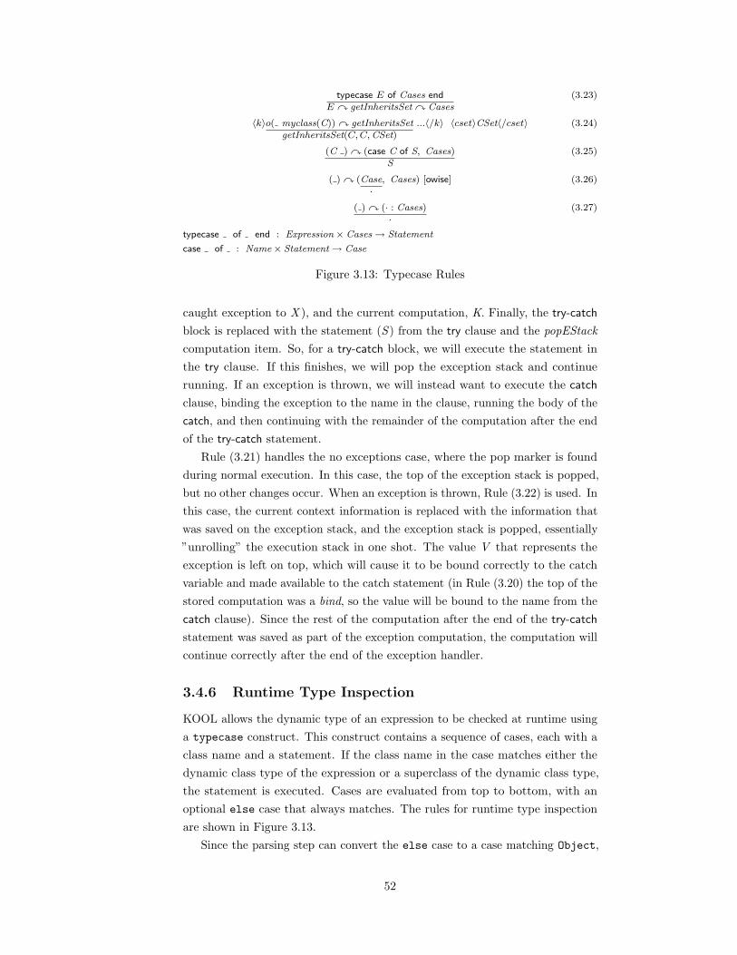
typecase E of Cases endE y getInheritsSet y Cases
(3.23)
〈k〉o( myclass(C)) y getInheritsSetgetInheritsSet(C, C,CSet)
...〈/k〉 〈cset〉CSet〈/cset〉 (3.24)
(C ) y (case C of S, Cases)S
(3.25)
( ) y (Case·
, Cases) [owise] (3.26)
( ) y (· : Cases)·
(3.27)
typecase of end : Expression× Cases→ Statement
case of : Name× Statement→ Case
Figure 3.13: Typecase Rules
caught exception to X ), and the current computation, K. Finally, the try-catch
block is replaced with the statement (S ) from the try clause and the popEStack
computation item. So, for a try-catch block, we will execute the statement in
the try clause. If this finishes, we will pop the exception stack and continue
running. If an exception is thrown, we will instead want to execute the catch
clause, binding the exception to the name in the clause, running the body of the
catch, and then continuing with the remainder of the computation after the end
of the try-catch statement.
Rule (3.21) handles the no exceptions case, where the pop marker is found
during normal execution. In this case, the top of the exception stack is popped,
but no other changes occur. When an exception is thrown, Rule (3.22) is used. In
this case, the current context information is replaced with the information that
was saved on the exception stack, and the exception stack is popped, essentially
”unrolling” the execution stack in one shot. The value V that represents the
exception is left on top, which will cause it to be bound correctly to the catch
variable and made available to the catch statement (in Rule (3.20) the top of the
stored computation was a bind, so the value will be bound to the name from the
catch clause). Since the rest of the computation after the end of the try-catch
statement was saved as part of the exception computation, the computation will
continue correctly after the end of the exception handler.
3.4.6 Runtime Type Inspection
KOOL allows the dynamic type of an expression to be checked at runtime using
a typecase construct. This construct contains a sequence of cases, each with a
class name and a statement. If the class name in the case matches either the
dynamic class type of the expression or a superclass of the dynamic class type,
the statement is executed. Cases are evaluated from top to bottom, with an
optional else case that always matches. The rules for runtime type inspection
are shown in Figure 3.13.
Since the parsing step can convert the else case to a case matching Object,
52
we assume in the semantics that there is no longer a designated else case.
When a typecase is encountered, Rule (3.23) shows that this is replaced with
an evaluation of the expression E, on top of the getInheritsSet computation
item, followed by the Cases that will be checked. When the expression E is
evaluated to an object value, Rule (3.24) shows the start of building the set of
class names that will be used in the check against the cases. The getInheritsSet
computation item is changed to another item with the same name but three
parameters, a class name, a set of class names and a set of classes, with the first
two parameters set to the dynamic class of the expression result, C. The inherits
set is built according to the rules in Figure 3.7.
With the set of classes for the expression calculated, the remaining three
rules, Rules (3.25), (3.26) and (3.27), process the cases. In the first, a matching
case in the set of cases (the rest of the set is ) is found, so the class name set
(C ) and the remainder of the cases list are both discarded, replaced by the
statement S from the matched case. In the second, the case does not match, but
there are cases left in the list, so the current case is removed, allowing the next
to be tried. In the third, there are no cases left in the list, so both the cases
list and the class name set are discarded, allowing control to fall through to
whatever was after the case statement. This provides for the intended semantics
– the statement of the first matching case (if any) will execute, then control will
pick up with the next statement after the end of the typecase.
3.4.7 Primitives
Since all operations are modeled as message sends, there isn’t a native way in
the language to, for instance, add two numbers, or output a string. Yet, at
some point, 5 + 3 actually has to yield 8. This is done using primitives, a
concept similar to that used in Smalltalk. Each class which is used to represent
a primitive value, such as Integer, is declared as a primclass, which adds a
field that stores the primitive value. This field can be accessed by the primitive
operations to either take out the existing primitive value or put a new one in.
For instance, for 5 + 3, primitive operations would take out the value 5 and the
value 3, add them using the system version of integer addition, create a new
Integer object, and put the primitive value 8 into the new object’s primitive
value field. All “system” operations, including input and output, are handled
using primitives, providing the programmer with an object-level view of the
primitive operations.
3.5 Adding Concurrency
The dynamic semantics from Section 3.4 does not support any concurrent
operations – as defined, KOOL is a sequential language, with a single thread
of execution. In this section language prototyping is illustrated by extending
53

Statement S ::= ... | spawn E ; | acquire E ; | release E ;
Figure 3.14: KOOL Syntax Extensions for Concurrency
KOOL with native support for concurrency. There are many different options
for how concurrency can be supported. The model chosen here is simple on
purpose, but still provides enough flexibility to create programs with multiple
concurrent threads and thread synchronization operations.
To support concurrency, a new statement, spawn, is added to the syntax to
allow the creation of new threads. Threads will be able to acquire and release
locks on specific objects (similarly to the basic locking functionality in the Java
language) using acquire and release statements. Finally, the semantics should
correctly model the accesses to shared memory locations, which should compete –
if two threads both assign a value to a shared variable, the resulting value should
be nondeterministic, based on the actual execution order of the threads.
With multiple threads, and thus multiple concurrent streams of execution,
some of the state components will need to be duplicated. This includes any
components which provide context to the current thread of execution: the current
object, the current class, the entire control, and the environment. This allows
each thread to have enough local information to execute without interfering
with the execution of other threads. For instance, threads should not share the
current class, since a message send in one thread would potentially interfere with
a message send in the other if they did. However, some information, such as the
Config
StringList
ControlEnvironment
StringList
Store
ClassSet
MethodStack ExceptionStack LoopStackComputation
Value Name
cset
mem
output
input
k mstack estacklstack
Nat
nextloc
Thread
env controlcobj
cclass
t*
LockSet
LockTupleSet
busy
holds
NameNat
lbl tid
Nat
nextTid
Threads
threads
Nat
Bool
tc
aflag
Figure 3.15: KOOL State Infrastructure, Extended for Concurrency
54

eval(Classes E,SL)newThrd(E, ·, ·, ·) 〈mem〉·〈/mem〉 〈nextLoc〉0〈/nextLoc〉 〈busy〉·〈/busy〉〈cset〉process(Classes)〈/cset〉 〈input〉SL〈/input〉 〈output〉·〈/output〉
(3.28)
〈t〉〈k〉spawn E·
...〈/k〉 〈env〉Env〈/env〉 〈cobj〉O〈/cobj〉 〈cclass〉C〈/cclass〉 ...〈/t〉
·newThrd(E,Env, O, C)
(3.29)
newThrd(E,Env, O, C)〈t〉〈control〉〈k〉E〈/k〉 〈mstack〉·〈/mstack〉 〈estack〉·〈/estack〉 〈lstack〉·〈/lstack〉〈/control〉
〈env〉Env〈/env〉 〈cobj〉O〈/cobj〉 〈cclass〉C〈/cclass〉 〈holds〉·〈/holds〉〈/t〉(3.30)
〈t〉〈k〉·〈/k〉 〈holds〉LTS〈/holds〉 ...〈/t〉·
〈busy〉 LSLS− LTS
〈/busy〉 (3.31)
spawn : Expression→ Statement
acquire : Expression→ Statement [strict]
release : Expression→ Statement [strict]
Figure 3.16: Concurrent KOOL Rules, Part 1
set of classes and the store, will be global to all threads. Figure 3.15 shows the
configuration from Figure 3.6 extended to enable concurrency.
The additional syntax and new rules for the dynamic semantics for concur-
rency in KOOL are shown in Figures 3.14, 3.16, and 3.17. It is important to
note that, even with fairly significant changes to the configuration and to the
language functionality, most of the rules are new – the only changed rule is Rule
(3.28), used for program evaluation, which does change to take account of the
new state infrastructure. This is the concurrent version of Rule (3.9). Rule
(3.28) makes use of the newThrd computation item to create a new execution
thread and set up the starting state appropriately.
The spawn statement creates a new thread based on a provided expression.
The expression is evaluated in the new thread, meaning any exceptions thrown
by the expression when it is evaluated will be handled in the new, not the
spawn’ing, thread. This is a design decision, and has been made to simplify the
semantics; an earlier version of this rule assumed that only method calls could be
spawned, and evaluated all method arguments in the current thread, providing
different exception behavior. Rule (3.29) shows the semantics of spawn. Here,
the expression E in the spawn statement is given to the newThrd item, along
with the current environment(Env), the current object (O), and the current
class(C ). spawn returns no value, so it is just removed from the computation.
Rule (3.30) shows how the new thread is actually created. The passed values
for expression, environment, object, and class are plugged into the proper state
components nested within the new thread. This will start the new thread for
expression E running in the proper environment. When the thread finishes, it
needs to be removed, with any locks it holds being removed from the global busy
lock set. This is illustrated in Rule (3.31).
Along with the ability to create new threads, we also need to be able to
55

acquire and release locks. This is done using the acquire and release statements.
The semantics for acquire is shown in Rules (3.32) and (3.33). In Rule (3.32), a
lock is acquired on an object V that the current thread already holds a lock on.
This just increments the lock count on this object from N to the successor of N.
In Rule (3.33), a lock is acquired on a value V that no thread, including the
current thread, has a lock on. This adds the value V and a lock count of 1 to the
thread’s holds set, while also adding V to the current global lock set LS. The
lock count in holds is necessary to ensure that lock acquires and releases are
balanced – a thread can acquire a lock multiple times, with a recursive method
call for instance, and we need to ensure that a lock is not inadvertently released
too soon.
The semantics for release is shown in Rules (3.34), (3.35), and (3.36). In rule
(3.34), a lock on value V with lock count 1 is released. This removes the lock
from both the local holds set and the global busy set. Rule (3.35) shows what
happens when a lock on value V with lock count greater than 1 is released –
here, the count simply goes from s(N) (the successor of N) to N . Finally, if
there is an attempt to release a lock that the thread does not hold, an exception
should be thrown. This is shown in Rule (3.36), where an attempt to release a
lock on V not held by the thread results in a LockNotHeldEx exception being
thrown.
A sample concurrent program, the thread game, is shown in Figure 3.18. In
this program a new class, ThreadGame, is defined. The constructor for this class
sets field x to the value 1. The Add method then includes an infinite loop that,
during each execution of the loop body, issues a single statement, adding x to x
and assigning the result back to x.
If this program were not concurrent, this would just double the value of x
each time through the loop. However, the Run method spawns two threads, each
of which will execute the Add method. Because there is no synchronization used
to prevent data races, the two threads can easily interfere with one another. In
〈k〉(acquire V·
...〈/k〉 〈holds〉... (V, Ns(N)
) ...〈/holds〉 (3.32)
〈k〉(acquire V·
...〈/k〉 〈holds〉... ·(V, 1)
...〈/holds〉 〈busy〉... LSLS V
...〈/busy〉 if V /∈ LS (3.33)
〈k〉(release V·
...〈/k〉 〈holds〉... (V, 1)·
...〈/holds〉 〈busy〉... V·
...〈/busy〉 (3.34)
〈k〉(release V·
...〈/k〉 〈holds〉... (V, s(N)N
) ...〈/holds〉 (3.35)
〈k〉( release Vthrow new LockNotHeldEx
...〈/k〉 〈holds〉LTS〈/holds〉 [owise] (3.36)
spawn : Expression→ Statement
acquire : Expression→ Statement [strict]
release : Expression→ Statement [strict]
Figure 3.17: Concurrent KOOL Rules, Part 2
56

class ThreadGame is
var x;
method ThreadGame is
x <- 1;
end
method Add is
while true do x <- x + x; od
end
method Run is
spawn(self.Add); spawn(self.Add);
end
end
(new ThreadGame).Run
./runkool examples/ThreadGame.kool -t 10
... term omitted ...
Solution 1 (state 2294)
states: 3381 rewrites: 310427 in 14388ms cpu
SL:[StringList] --> "10"
Figure 3.18: The Thread Game in KOOL
fact, it has been proved that the variable x can take the value of any natural
number greater than 0 [139]. Figure 3.18 also shows a sample run which checks
to see if the value 10 is reachable; this is found after generating 3381 reachable
states.
3.6 Other Extensions
Because of its use in our language research and in teaching, the KOOL system has
been designed to be extensible. This section illustrates two additional extensions
to KOOL: synchronized methods and label statements.
Method M ::= synchronized method X is D∗ S end |
synchronized method X ({X ′,}+ ) is D∗ S end
Statement S ::= X:
Figure 3.19: KOOL Syntax, Additional Extensions
57

method X (Xs) is Ds S end (3.37)
S y nil y return (3.38)
syncmethod X (Xs) is Dls S end (3.39)
self y acquireMthd y S y nil y return (3.40)
V y acquireMthdV y acquire y V y addELock y V y addMLock
(3.41)
Figure 3.20: Synchronized Methods
3.6.1 Synchronized Methods
As shown in Section 3.5, the KOOL language has a fairly simple model of
concurrency based on threads and object locks. synchronized methods, similar
to those in Java, would provide a higher-level abstraction over these locking
primitives. In Java, methods tagged with the synchronized keyword implicitly
lock the object that is the target of the method call, allowing only one thread
to be active in all synchronized methods on a given object at a time. We will
assume the same semantics for KOOL.
The syntax changes to add synchronized methods are minor: the keyword
needs to be added to the method syntax, which then also needs to be reflected
in the Maude-level syntax for KOOL. The extended concrete syntax for methods
is shown in Figure 3.19. The abstract syntax is similar, with a new method
operator, syncmethod:
op syncmethod_‘(_‘)is__end : Name Names Decls Stmt -> Method .
The changes to the semantics are obviously more involved. In KOOL, as in
Java, synchronized methods should work as follows:
• a call to a synchronized method should implicitly acquire a lock on the
message target before the method body is executed;
• a return from a synchronized method should release this lock;
• additional calls to synchronized methods on the same target should be
allowed in the same thread;
• exceptional returns from methods should release any locks implicitly ac-
quired when the method was called.
A quick survey of these requirements shows that adding synchronized
methods will change more than the message send semantics – the semantics for
exceptions will need to change as well, to account for the last requirement.
To handle the first requirement, a new lock can be acquired on the self object
at the start of any synchronized method simply by adding a lock acquisition
to the start of the method body, which can be done when the method definition
58
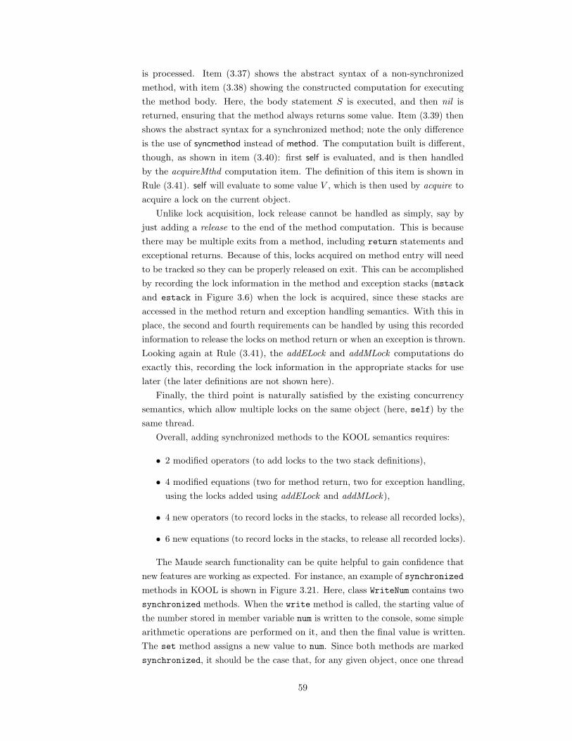
is processed. Item (3.37) shows the abstract syntax of a non-synchronized
method, with item (3.38) showing the constructed computation for executing
the method body. Here, the body statement S is executed, and then nil is
returned, ensuring that the method always returns some value. Item (3.39) then
shows the abstract syntax for a synchronized method; note the only difference
is the use of syncmethod instead of method. The computation built is different,
though, as shown in item (3.40): first self is evaluated, and is then handled
by the acquireMthd computation item. The definition of this item is shown in
Rule (3.41). self will evaluate to some value V , which is then used by acquire to
acquire a lock on the current object.
Unlike lock acquisition, lock release cannot be handled as simply, say by
just adding a release to the end of the method computation. This is because
there may be multiple exits from a method, including return statements and
exceptional returns. Because of this, locks acquired on method entry will need
to be tracked so they can be properly released on exit. This can be accomplished
by recording the lock information in the method and exception stacks (mstack
and estack in Figure 3.6) when the lock is acquired, since these stacks are
accessed in the method return and exception handling semantics. With this in
place, the second and fourth requirements can be handled by using this recorded
information to release the locks on method return or when an exception is thrown.
Looking again at Rule (3.41), the addELock and addMLock computations do
exactly this, recording the lock information in the appropriate stacks for use
later (the later definitions are not shown here).
Finally, the third point is naturally satisfied by the existing concurrency
semantics, which allow multiple locks on the same object (here, self) by the
same thread.
Overall, adding synchronized methods to the KOOL semantics requires:
• 2 modified operators (to add locks to the two stack definitions),
• 4 modified equations (two for method return, two for exception handling,
using the locks added using addELock and addMLock),
• 4 new operators (to record locks in the stacks, to release all recorded locks),
• 6 new equations (to record locks in the stacks, to release all recorded locks).
The Maude search functionality can be quite helpful to gain confidence that
new features are working as expected. For instance, an example of synchronized
methods in KOOL is shown in Figure 3.21. Here, class WriteNum contains two
synchronized methods. When the write method is called, the starting value of
the number stored in member variable num is written to the console, some simple
arithmetic operations are performed on it, and then the final value is written.
The set method assigns a new value to num. Since both methods are marked
synchronized, it should be the case that, for any given object, once one thread
59
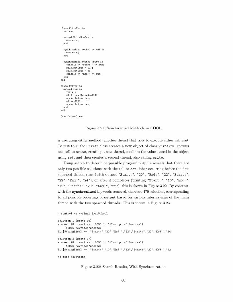
class WriteNum isvar num;
method WriteNum(n) isnum <- n;
end
synchronized method set(n) isnum <- n;
end
synchronized method write isconsole << "Start:" << num;self.set(num + 10);self.set(num - 8);console << "End:" << num;
endend
class Driver ismethod run is
var w1;w1 <- new WriteNum(10);spawn (w1.write);w1.set(20);spawn (w1.write);
endend
(new Driver).run
Figure 3.21: Synchronized Methods in KOOL
is executing either method, another thread that tries to execute either will wait.
To test this, the Driver class creates a new object of class WriteNum, spawns
one call to write, creating a new thread, modifies the value stored in the object
using set, and then creates a second thread, also calling write.
Using search to determine possible program outputs reveals that there are
only two possible solutions, with the call to set either occurring before the first
spawned thread runs (with output "Start:", "20", "End:", "22", "Start:",
"22", "End:", "24"), or after it completes (printing "Start:", "10", "End:",
"12", "Start:", "20", "End:", "22"); this is shown in Figure 3.22. By contrast,
with the synchronized keywords removed, there are 470 solutions, corresponding
to all possible orderings of output based on various interleavings of the main
thread with the two spawned threads. This is shown in Figure 3.23.
> runkool -s --final Sync5.kool
Solution 1 (state 96)
states: 98 rewrites: 10390 in 612ms cpu (612ms real)
(16976 rewrites/second)
SL:[StringList] --> "Start:","20","End:","22","Start:","22","End:","24"
Solution 2 (state 97)
states: 98 rewrites: 10390 in 612ms cpu (612ms real)
(16976 rewrites/second)
SL:[StringList] --> "Start:","10","End:","12","Start:","20","End:","22"
No more solutions.
Figure 3.22: Search Results, With Synchronization
60

> runkool -s --final Sync6.kool
Solution 1 (state 80383)
states: 80853 rewrites: 10112671 in 671633ms cpu (674345ms real)
(15056 rewrites/second)
SL:[StringList] --> "Start:","20","End:","22","Start:","22","End:","24"
...
Solution 470 (state 80852)
states: 80853 rewrites: 10112671 in 671645ms cpu (674360ms real)
(15056 rewrites/second)
SL:[StringList] --> "Start:","10","End:","Start:","20","End:","22","12"
No more solutions.
Figure 3.23: Search Results, Without Synchronization
3.6.2 Labels
To make it easier to write LTL formulae that refer to positions within a program,
label statements have been added to KOOL. A label statement is just an identifier
followed by a colon, such as X:. When a label is encountered, a cell, at the
thread level, that holds the current label is changed, allowing the change to be
captured in a proposition defined as part of KOOL’s model checking support.
This is shown in Figure 3.24, Rule (3.42).
In Maude, this is supported using the following model checking proposition:
op labeled : Nat Name -> Prop .
eq t(tid(N) lbl(X) TS) S |= labeled(N,X) = true .
3.7 KOOL Implementation
KOOL programs are generally run using the runkool script, since running a
KOOL program involves several steps and tools, and since programs can be run
in different modes (execution, search, and model checking, each with various
options). First, the KOOL prelude, a shared set of classes for use in user
programs, is added to the input program. This program is then parsed using
the SDF parser [193], which takes the program text and a syntax definition file
as input. The parser produces a file in ATerm format, an SDF format used
to represent the abstract syntax tree. A pretty printer then converts this into
Maude, using prefix versions of the operators to prevent parsing difficulties.
Finally, Maude is invoked by runkool with the language semantics and the
〈k〉label(X)·
...〈/k〉 〈lbl〉X〈/lbl〉 (3.42)
Figure 3.24: Label Statements
61
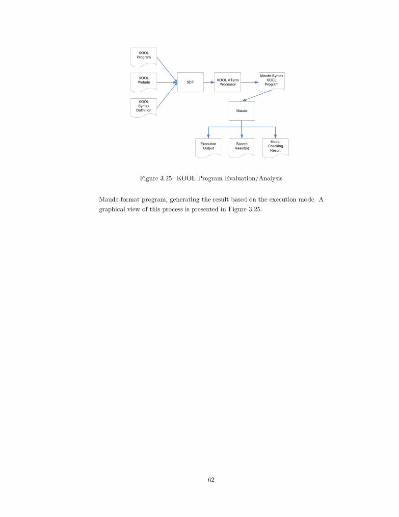
KOOL
Program
KOOL
Prelude SDF
KOOL
Syntax
Definition
KOOL ATerm
Processor
Maude-Syntax
KOOL
Program
Maude
Execution
Output
Search
Result(s)
Model
Checking
Result
Figure 3.25: KOOL Program Evaluation/Analysis
Maude-format program, generating the result based on the execution mode. A
graphical view of this process is presented in Figure 3.25.
62
Chapter 4
A Prototype of Beta
KOOL was designed using prototyping techniques, and was also designed as a
platform for experimenting with language features. To show that the techniques
used for experimenting with the KOOL definition can also be used for program-
ming languages not designed with these techniques in mind, this chapter presents
parts of a definition of the Beta language [121]. At the time this material was
being written the Beta definition was being modified to take advantage of tech-
niques developed over the last few years in K and rewriting logic semantics. The
version presented here is based on an earlier version of the language definition
[83], although the semantic rules show here are presented using the newer K
format. Information about the version currently being developed can be found
online at the FSL Beta language website [82].
4.1 The Beta Language
Beta is an object-oriented language developed as the successor to the Simula 67
language [156]. It is probably best known for two features that set it apart from
more commonly used object-oriented languages, such as C++ and Java:
• Beta has collapsed the concepts of class and method into a single concept,
the pattern. A pattern consists of local variable declarations, input param-
eters (the enter block), output parameters (the exit block), and actions
(the do block). Instances of patterns are created to represent objects,
execute as methods, etc.
• To invoke inherited but overridden functionality, most object-oriented
languages provide a super-call mechanism. Beta does the opposite: method
dispatch always starts at the top of the inheritance hierarchy, and then
heads down the hierarchy towards the actual pattern using inner calls.
This provides a method to enforce behavioral subtyping [117], since a
parent pattern can either choose not to invoke a child pattern, or can at
least ensure that necessary invariants still hold after the child executes.
Both of these features, along with a number of interesting, yet more com-
mon, language features, such as deterministic alternation (i.e., coroutines) and
concurrency, make Beta a challenging language to correctly define.
63

4.2 Beta Semantics
The dynamic semantics of Beta are specified using K, translated into Maude
to provide an environment for program evaluation and analysis. In this section
several of the more interesting features of the definition are presented. The
remainder of the definition is available on the FSL Beta website [82].
4.2.1 Method Dispatch Semantics
Similar to C++, Beta provides both static and dynamic dispatch for invocations
of patterns used like methods. Standard pattern declarations make use of a
colon to separate the name of the pattern from the implementation1:
DisplayReservation:
(#
do Date.Display; Customer.Display; INNER
#);
Virtual patterns use similar notation, with :< indicating that a pattern is being
made virtual in this pattern and all inheriting patterns:
Display:< DisplayReservation
In child patterns that provide a new version of the virtual pattern, the notation
::< is used instead. This first example provides a new version of the Display
pattern, in this case overridden to properly handle displaying train reservations:
DisplayTrainReservation: DisplayReservation
(#
do ReservedTrain.Display;
ReservedCarriage.Display;
ReservedSeat.Display;
INNER
#);
Display::< DisplayTrainReservation
The second example provides a different extension of the basic reservation display
functionality, this time for flights:
DisplayFlightReservation: DisplayReservation
(#
do ReservedFlight.Display;
ReservedSeat.Display;
1The sample code shown in this section is from the book “Object-Oriented Programmingin the BETA Programming Language”, by Madsen, Møller-Pedersen, and Nygaard [121]
64
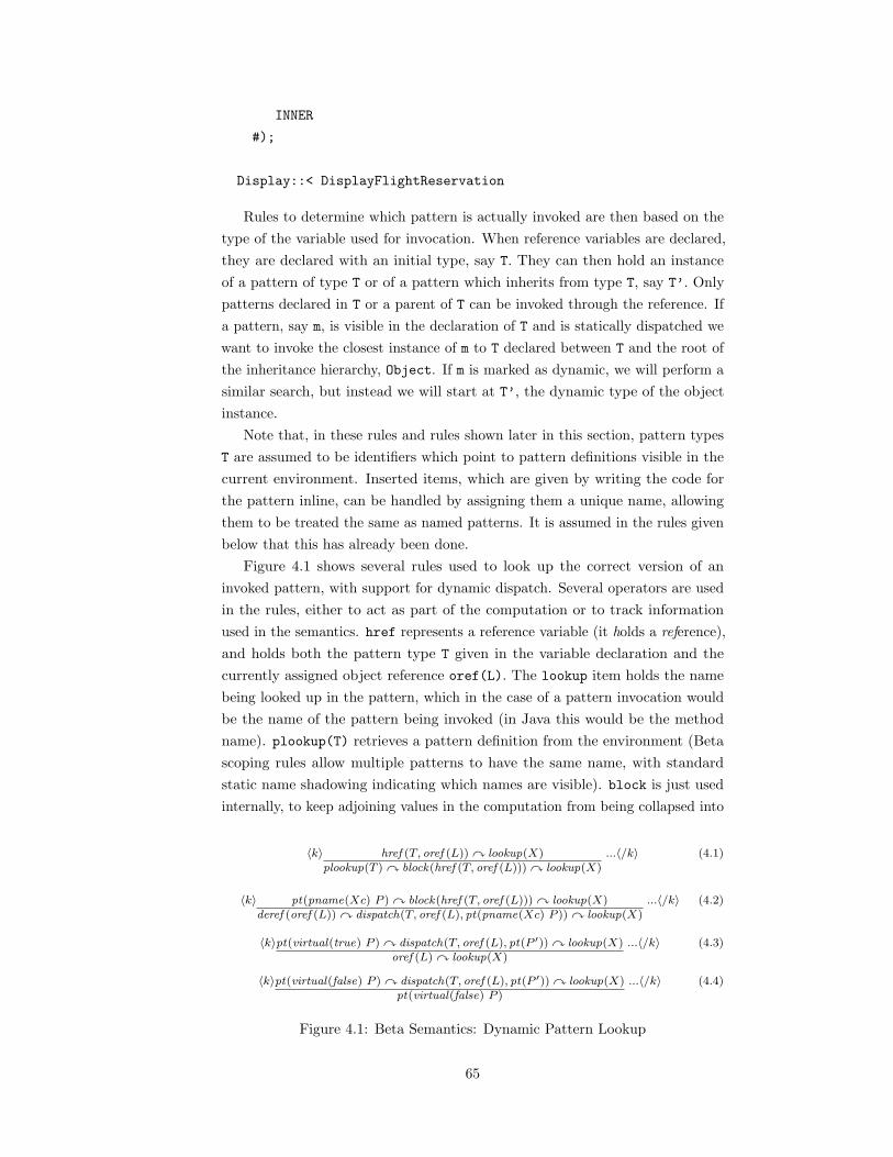
INNER
#);
Display::< DisplayFlightReservation
Rules to determine which pattern is actually invoked are then based on the
type of the variable used for invocation. When reference variables are declared,
they are declared with an initial type, say T. They can then hold an instance
of a pattern of type T or of a pattern which inherits from type T, say T’. Only
patterns declared in T or a parent of T can be invoked through the reference. If
a pattern, say m, is visible in the declaration of T and is statically dispatched we
want to invoke the closest instance of m to T declared between T and the root of
the inheritance hierarchy, Object. If m is marked as dynamic, we will perform a
similar search, but instead we will start at T’, the dynamic type of the object
instance.
Note that, in these rules and rules shown later in this section, pattern types
T are assumed to be identifiers which point to pattern definitions visible in the
current environment. Inserted items, which are given by writing the code for
the pattern inline, can be handled by assigning them a unique name, allowing
them to be treated the same as named patterns. It is assumed in the rules given
below that this has already been done.
Figure 4.1 shows several rules used to look up the correct version of an
invoked pattern, with support for dynamic dispatch. Several operators are used
in the rules, either to act as part of the computation or to track information
used in the semantics. href represents a reference variable (it holds a reference),
and holds both the pattern type T given in the variable declaration and the
currently assigned object reference oref(L). The lookup item holds the name
being looked up in the pattern, which in the case of a pattern invocation would
be the name of the pattern being invoked (in Java this would be the method
name). plookup(T) retrieves a pattern definition from the environment (Beta
scoping rules allow multiple patterns to have the same name, with standard
static name shadowing indicating which names are visible). block is just used
internally, to keep adjoining values in the computation from being collapsed into
〈k〉 href (T, oref (L)) y lookup(X)plookup(T ) y block(href (T, oref (L))) y lookup(X)
...〈/k〉 (4.1)
〈k〉 pt(pname(Xc) P ) y block(href (T, oref (L))) y lookup(X)deref (oref (L)) y dispatch(T, oref (L), pt(pname(Xc) P )) y lookup(X)
...〈/k〉 (4.2)
〈k〉pt(virtual(true) P ) y dispatch(T, oref (L), pt(P ′)) y lookup(X)oref (L) y lookup(X)
...〈/k〉 (4.3)
〈k〉pt(virtual(false) P ) y dispatch(T, oref (L), pt(P ′)) y lookup(X)pt(virtual(false) P )
...〈/k〉 (4.4)
Figure 4.1: Beta Semantics: Dynamic Pattern Lookup
65

a value list. The deref item retrieves the actual object stored at the location
pointed to by oref(L), and dispatch keeps track of the information we need for
pattern dispatch: the type T, the object reference oref(L) we are dispatching
to, and the pattern pt(P’) that defines the type T.
With all this in mind, the rules in Figure 4.1 can now be understood. In Rule
(4.1), when we are looking up a name (say m) via a reference (say with static
type T), we first get back the pattern that defines type T. In Rule (4.2), with the
pattern for T available, we use deref to retrieve the referenced object and store
the information we will need to perform the pattern dispatch later, once the
actual object has been retrieved. A rule not shown here uses the retrieved object
to find the first definition of m at the level of T or above (towards Object).
Rules (4.3) and (4.4) then trigger the correct dispatch. In Rule (4.3), if the
definition of m states that it is virtual, we will again look up m, but this time
we will use the dynamic type of the referenced object, not the static (declared)
type of the reference. In Rule (4.4), where virtual is false, we have already found
the pattern that will be instantiated by this call, so we can just return that. In
both cases, the expectation is that a pattern will be returned, which will be
instantiated to invoke the pattern code.
4.2.2 Pattern Membership Semantics
In Beta, variables can be queried for the pattern they instantiate. This is called
pattern membership and can be used to test (say, in a conditional with multiple
branches) whether an object is an instance of one of several patterns:
(if R##
// TrainReservation## then NTR+1->NTR
// FlightReservation## then NFR+1->NFR
if)
Here, the ## operator is used with variable R to determine its pattern; the
same operator is then used inside the conditional (the Beta conditional, in its
general form, uses a number of cases, each preceded by //) in two branches,
one branch testing to see if R is of pattern type TrainReservation, the other
testing to see if R is of pattern type FlightReservation.
Figure 4.2 shows rules used to retrieve the pattern. Rule (4.5) provides the
initial rule used by the ## operator: given E ##, E is evaluated, and the pattern
used to define E is then retrieved. Rules (4.6) and (4.7) handle the case where
E is an object reference. In Rule (4.6), when an object reference is returned,
the reference is dereferenced to retrieve the actual object. In Rule (4.7), once
this object is retrieved, the object’s myPattern attribute is used to get back the
actual pattern used to define the object. The use of plookup will retrieve the
pattern itself. In Rule (4.8), the lookup resulted directly in a pattern (this would
happen in cases such as FlightReservation ##), in which case that pattern is
returned.
66

〈k〉 E ##E y getPattern
...〈/k〉 (4.5)
〈k〉 oref (L) y getPatternderef (oref (L)) y getPattern
...〈/k〉 (4.6)
〈k〉o(myPattern(T ) ) y getPatternplookup(T )
...〈/k〉 (4.7)
〈k〉pt(P ) y getPatternpt(P )
...〈/k〉 (4.8)
Figure 4.2: Beta Semantics: Pattern Membership
4.2.3 Code as Values Semantics
In Beta it is not only possible to determine the pattern of an expression, it is also
possible to treat patterns as values which can be assigned to pattern variables
and then instantiated like any other pattern. To do this, we can leverage other
parts of the language definition, including definitions for assignment and pattern
membership.
Rule (4.9) provides the base semantics for creating a pattern variable as an
extension of other rules for creating declarations (not shown), which also use the
createDec computation. Given a pattern type T, a new variable using operator
pvar is created. This is similar to href, holding both the declared type of the
pattern variable, which constrains what can be held, and the actual pattern,
initially set to nothing.
Rule (4.10) extends the pattern membership test logic, discussed earlier, with
support for pattern variables. Rule (4.11) then provides an extension to the logic
used to look up a pattern for invocation, allowing pattern variables to be used
in place of explicit pattern names. Finally, Rules (4.12) and (4.13) provide logic
to handle assignments to pattern variables. Rule (4.12) triggers evaluation of
both sides of the assignment (the assignment target is to the right of the arrow),
indicating that this should be an assignment to a pattern variable. Rule (4.13)
then specifies the logic used to assign the pattern: given an existing pattern
variable pvar, and given that E evaluated to pattern P, pattern P is saved inside
〈k〉createDec(##T )pvar(T,nothing)
...〈/k〉 (4.9)
〈k〉pvar(T, V ) y getPatternV
...〈/k〉 (4.10)
〈k〉pvar(T, pt(P )) y lookupForInvokept(P ) y lookupForInvoke
...〈/k〉 (4.11)
〈k〉 E → (X ##)(E, X) y assignToPVar(X) y nothing
...〈/k〉 (4.12)
〈k〉(pt(P ), pvar(T, )) y assignToPVar(X)pvar(T, pt(P )) y assignTo(X)
...〈/k〉 (4.13)
Figure 4.3: Beta Semantics: Code as Values
67

〈t〉 〈k〉 saveAndRecoverStack(V l) y KfrozenState(K,Env ,TS) y assignToLoc(L) y V l y K′
〈/k〉 〈env〉EnvEnv ′
〈/env〉
〈altloc〉LL′
〈/altloc〉 〈altstate〉(K′,Env ′, L′, TS′′, TS′)TS′′
〈/altstate〉 TSTS′
〈/t〉 (4.14)
Figure 4.4: Beta Semantics: Deterministic Alternation
the pvar, which is then assigned back to X.
4.2.4 Deterministic Alternation Semantics
The Beta deterministic alternation functionality allows Beta to support corou-
tines. Instead of using multiple threads, with objects running concurrently,
different objects run inside the same thread, with each object running until it
either finishes its do block or issues a suspend call.
The most interesting part of the alternation semantics deal with suspending
an object and restarting it later. The semantics to do this are shown in Rule
(4.14) in Figure 4.4.
This rule is triggered by a suspend call; a similar equation handles the restart.
When suspended, the current execution stack needs to be saved, and the prior
stack recovered. Several pieces of state information help with this process.
altloc contains the memory location of the variable that holds the alternating
object, which will need to be updated to hold the altered state. altstate
contains the thread state that was current when the alternating execution of this
object was started, which is the state that needs to be recovered to correctly
handle the suspend. Note that it contains similar information to the current
matched context, including its own version of the altstate, allowing nested
alternations to be properly represented.
Now, using these parts of the configuration, the rule takes the current pieces
of state that need to be saved at suspend, including the current computation
(minus the saveAndRecoverStack item), current environment, and other parts
of the thread state; puts these into a frozenState item; and assigns them back
to the location holding the alternating object that is currently executing. Next,
the remainder of the current computation is switched for the saved computation
stored in altstate (suspending also passes back the exit values for the pattern,
hence the need for Vl on top of the computation). At the same time, the rule
recovers the old environment, altloc, and altstate, along with other thread
state information, ensuring that when the computation continues it is back in
the correct state.
68
4.3 Beta Implementation
The version of the Beta semantics [83] described in this chapter uses an encoding
of the Beta syntax directly into Maude notation, using Maude sorts, operations,
and operator precedences. This has the advantage of allowing Beta programs
to be written directly as Maude terms in a Beta-like syntax. However, it is
also limiting in two ways. First, to allow Maude to disambiguate language
constructs that look similar, it is often necessary to either add a large number
of parentheses to programs or modify the syntax, giving different language
constructs distinct syntactical representations. Second, it is not possible to take
actual Beta programs and run them directly in the semantics, since they first
have to be converted to work with the Maude version of the syntax.
The version of the Beta semantics currently being developed instead uses the
Beta metaprogramming capabilities to define a Beta lexer, parser, and pretty-
printer. The pretty-printer generates terms using a Maude-defined abstract
syntax of Beta, transforming the constructs into the prefix versions of the defined
mixfix syntax2. By moving complex parsing outside of Maude, it is possible
to use syntax closer to the actual Beta language when writing rules, while
eliminating the cumbersome process of defining precedences in Maude. It is
also possible to process actual Beta programs directly, making it easier to use
the definition. Outside of these parsing and pretty-printing capabilities, the
remainder of the system in the version currently being developed, including all
semantics and analysis tools, is written in Maude.
4.4 Extending Beta
One goal of the work on language prototyping is to provide an environment where
changes to a language can be implemented quickly, allowing for experimentation
with new language features. As an example, we decided to add super calls to
the Beta language, taking our inspiration from similar work [72] which added
inner calls to a Java-like object system in MzScheme. Since Beta has both
static and virtual pattern dispatch, we have started by just adding this to static
calls, but we believe it would be fairly straight-forward to also add this feature
to dynamic calls. We also have restricted this feature to named patterns only –
it doesn’t seem as useful to allow this with anonymous patterns, since we cannot
use an anonymous pattern as a parent to other patterns.
To add super calls, we first added a new type of pattern, a Java pattern,
which can be the target of a super call. This required adding two syntax
operators: one for pattern declaration, to indicate that the pattern being defined
is a Java-style pattern; and one new expression, super, used the same as in
Java, to initiate a super-call. We then needed to add two operators to the
2It is always possible to use a mixfix operator in prefix form; one advantage of this is thatthe prefix form is easier for Maude to parse, while the mixfix form can still be used whenwriting equations and rules in the semantics
69

semantics as well: a boolean flag, stored as part of the information kept with
patterns, to specify whether the pattern is a Java-style or Beta-style pattern;
and a computation item, used as part of the pattern semantics to appropriately
set this boolean flag on newly created patterns.
In the language semantics, we changed a total of 9 rules and added 9 more.
Of the 9 that were changed:
• 5 were to initialize patterns to not be Java patterns by default, but to act
as standard Beta patterns;
• two were to properly handle building the inner call list used for pattern
invocations;
• one was to trigger pattern invocations to start at Object if the pattern
invocation is not of a Java pattern, i.e. to use standard Beta semantics;
• and one was to flag the Object pattern as a standard (not Java) Beta
pattern.
Of the 9 rules that were added:
• 2 were to enumerate fields in a pattern with the new Java pattern syntax;
• one was to ensure Java patterns are not added to the list for inner calls;
• one was to ensure that a pattern invocation of a Java pattern would start
at that pattern instead of at Object;
• two were to handle super calls;
• and three were to handle setting the Java flag on Java patterns.
Overall, it took roughly 2 hours to add this feature into our prior definition
of Beta. It has not yet been ported forward to the new definition, but plans are
to do so once the language definition is complete. The files with the extended
semantics, with examples with and without super, are available on the rewriting
logic semantics Beta website [82].
70

Chapter 5
The K Module System
One important aspect of formalisms for defining the semantics of programming
languages is modularity. Modularity is generally expressed as the ability to add
new language features, or modify existing features, without having to modify
unrelated semantic rules. For instance, when designing a simple expression
language, one may want to use structural operational semantics (SOS) [162] to
define the semantics of addition1:
e1 → e′1
e1 + e2 → e′1 + e2
(EXP-PLUS-L)
e2 → e′2
n1 + e2 → n1 + e′2(EXP-PLUS-R)
n1 + n2 → n, where n is the sum of n1 and n2 (EXP-PLUS)
Further extending the language, one may want to add variables. One way to
do this is to define an environment, mapping names to values, with rules for
binding values to names (not shown here) and to retrieve the value of a binding:
〈x, ρ〉 → 〈n, ρ〉,where n = ρ(x) (VAR-LOOKUP)
With this change to the language, even though the rules for plus do not actually
reference the environment they are still modified to include it as part of the
configuration. As an example, rule EXP-PLUS-L becomes:
〈e1, ρ〉 → 〈e′1, ρ〉
〈e1 + e2, ρ〉 → 〈e′1 + e2, ρ〉
(EXP-PLUS-L)
To accommodate other language features that require extensions to the
configuration, such as stores (for updatable memory locations) or mappings to
information about classes and methods (in an object-oriented language, especially
one where this information can change as the program runs, such as Self or
Python), similar changes are made to the same language features, even in cases
where they are not used directly in the rules. Alternatively, similar changes
1The same rules are used in Chapter 9
71
may need to be made to add addition expressions to a different language with a
different configuration, even if the different elements of the configuration are not
used in the rules for addition. All these changes are required because SOS is not
modular. Improved support for modularity eliminates the need to make these
changes, offering several advantages:
• Modular definitions of language features allow other parts of a language
to change more easily by allowing existing feature definitions to remain
unchanged in the face of unrelated modifications or additions;
• A modular definition of a language feature can be more easily reused
in the definition of a different language, even one with a much different
configuration;
• Modular definitions are easier to understand, since the rules given for a
language construct only need to include the information needed by the
rule, instead of including extraneous information used in other parts of the
language (such as the store in the rules for plus).
For these reasons, improving modularity of language definitions has been a
focus of research across multiple semantic formalisms. One example is modular
structural operational semantics (MSOS) [144, 146], which solves the problem
shown above by leveraging the labels on rule transitions, not normally used in
SOS definitions of programming languages, to encode configuration elements,
with the ability to elide unused parts of the configuration. This, and other
related work in modularity, is discussed in Chapter 9.
With a tool supported semantics, modularity can also be expressed as the
ability to package language features into discreet reusable units, which can then
be assembled when defining a language. The ability to create reusable language
feature modules requires having a modular semantics, since it should be possible
to plug the same feature into multiple language definitions, even in cases where
(unused) parts of the configuration are different. Additionally, it should be
possible to provide clean interfaces to language features and to different parts of
the configuration, something not required in monolithic definitions, or even in
modular definitions written on paper.
Context transformers, described in Section 2.5, are targeted towards the first
definition of modularity, allowing rules to remain unchanged as new features
are added and as the configuration used to represent the programming language
state is changed. The K module system, described here, is targeted towards the
second, providing a method to package up K definitions into modules which can
be stored in a shared repository and then reused when creating or modifying a
language definition. Section 5.1 provides an overview of the K module system,
introducing the basic constructs used when creating modules. Section 5.2 then
illustrates these concepts in the context of a number of short examples. To show
a more complete application, Section 5.3 provides an example of a complete,
72

albeit simple, kernel of the C language, which is then extended with a new
feature requiring changes to the configuration. Current K tool support uses
Maude; Section 5.4 provides details of the current translation from K modules
into a format usable by the current K implementation. Section 5.5 then discusses
the online semantics module repository, which includes client-side tools, built
around web services technology, and an initial XML document format designed
to allow the open exchange of semantics modules. Finally, Section 5.6 presents a
discussion of some of the challenges and limitations of the material presented
here and in the last two chapters.
5.1 K Modules
The K module system provides a general module format designed to allow the
definition of all features needed in a K language definition: abstract language
syntax, configuration items, semantic rules and equations, and the ultimate
assembly of a language, including the layout of the language configuration.
5.1.1 Module Notation
The module syntax is similar to that used in Maude, but with some simplifications
and some extensions to capture common language definition scenarios. The
notation is described below, grouped into constructs used in the module header
and in the module body.
Module Headers
A module header consists of the name of the module, a number of import, export,
and requires directives (one may include 0 or more of each), and a “wrapper”
around the module body items, starting with begin and ending with endmodule.
An overview of this notation is provided in Figure 5.1.
Module Name: In the K module system, module names are specified with
a full module path, a /-separated list of individual names. Examples of valid
module MODULE/NAME is
imports IMPORTS .
exports EXPORTS .
requires REQUIRES .
version VERSION# .
description "Arbitrary string." .
begin
module body items
endmodule
Figure 5.1: The Module Header
73

names would be INT, EXP/PLUS, and IMP/BEXP/AND. This use of paths provides a
way to logically group modules. For instance, all feature definitions representing
expressions could be given under EXP. Module names are not case sensitive,
although they are traditionally given using upper case alphanumeric characters.
The names are normalized inside the module system, so Exp, exp, and EXP are
all considered to be the same module.
As well as the main module path, a module name may include an optional
tag, indicating the type of module being defined. This tag is user-defined,
although two system-defined tags are also provided, SYNTAX and LANGUAGE.
These indicate that a module defines either the abstract syntax of a language
feature or an entire language, respectively. Examples include EXP/PLUS[SYNTAX]
and KOOL[LANGUAGE].
Imports: An imports clause indicates that a module depends on the defini-
tions provided in the imported module. imports is equivalent to the Maude
including; at this time there is no equivalent to either protecting or extending.
Following the keyword imports, one or more modules may be listed by module
path, each with an optional clause indicating modifications upon import. A
standard example of an imports clause is the following:
imports IMP/CONFIG/ENVIRONMENT .
Tags can also be provided on import paths:
imports IMP/EXP/PLUS[DYNAMIC] .
Imports also provide an optional renaming clause, indicating that names of sorts
or operations are being changed. The syntax for this clause is borrowed directly
from Maude, and has been extended to also allow additions of K attributes, such
as strict, to be defined on an operator on import. This allows an operator to
be initially defined without attributes such as strictness, since different semantics
may want to handle strictness in different ways.
### These represent a comment
### This import would be for a standard dynamic semantics,
### since we want to evaluate the guard but not the branches.
imports FUN/EXP/IF[SYNTAX]
* ( op if_then_else : Exp Exp Exp -> Exp now strict(1) ) .
### This import would be for a static semantics, where we need
### to check all branches.
imports FUN/EXP/IF[SYNTAX]
* ( op if_then_else : Exp Exp Exp -> Exp now strict ) .
74
Exports: An exports clause indicates that a module exports certain sorts,
operators or K cells:
exports sort Env, op _[_] : Env Id -> Loc, cell env(Env) .
If no exports clause is included in the module header, all sorts, operators, and
cells are exported from the module by default. If an exports clause is provided,
any sorts, operators, or cells not listed are considered private to just that module,
providing a method to create (for instance) local sorts and operations that do
not conflict with other sorts and operators in other modules which may share
the same name.
Requires: Using imports, it is possible for a module to include defined features,
including operations, sorts, and cells, given in another module. To defer the
decision of which module to import for these features ,they can instead be
listed in a requires clause. requires indicates that the features are used in
the current module, but that an actual definition will be provided later, inside
another module. For a module with a requires clause to be used in a language
definition, all its requirements must be met by one or more imported modules.
requires sort Env, op _[_] : Env Id -> Loc, cell env(Env) .
Version: The version number is optional, and is currently used only when
interacting with the module repository. The version number is in decimal format,
with up to three digits following the decimal point: numbers like 1, or 1.01 are
valid version numbers, but A3 or 1.1.3 are not.
Description: Like the version number, the description is optional, and is
currently only used with the module repository. The description can contain an
arbitrary string.
Module Bodies
The module body provides definitions of the items used in the syntax, semantics,
and configuration of a language. The various types of module body items that
can be defined are described below.
Sorts, Syntax Sorts, and Sort Aliases: Sort definitions in K modules use
the same syntax as sort definitions in Maude, with the keyword sort (or sorts)
followed by one or more identifiers naming the sort or sorts being defined:
sort Nat .
sorts Value ValueList .
75

To enable proper handling of definitional attributes such as strictness, it is
important that K modules make a distinction between sorts used to represent
abstract syntax and sorts used to represent non-syntax terms. Sorts defined
using sort are the latter; the keyword xsort, along with the variant xsorts,
define the former:
xsort Exp .
xsorts Stmt StmtList .
The K module system allows sort expressions using a number of built-in
sort constructors, including constructors for maps, lists, and sets. Sometimes
it is useful to define that a sort expression represents a specific concept, such
as a list of values or an environment. This makes definitions more readable
and provides better documentation, inside the definition, of the intent of the
semantics designer.
sortalias Env = KMap{Name,Loc} .
sortalias NumList = KList{Num} .
Subsorts: Subsorts are defined in K modules using the same syntax as provided
by Maude, with the < operator used to separate space-separated lists of one or
more sorts.
subsort A B C < D E < F G .
Ops and Syntax Ops: Operators are defined in K modules using syntax that
matches the syntax used in Maude. Like with sorts, it is important for K to be
able to distinguish between operators representing abstract syntax terms and
operators representing other operations in the semantics. This distinction is
made by using xop (with variant xops) for abstract syntax operators, and op
(ops) for the rest.
xop _+_ : Exp Exp -> Exp .
xop _:_?_ : Exp Exp Exp -> Exp .
op _[_] : Env Id -> Location .
Several extended attributes for operators are also supported by the K module
system. This includes strict, seqstrict, renameTo, dissolve, and aux. Other
attributes available in the K Maude syntax are represented by explicit construct
in the module system. For instance, the wrapping attribute, used in definitions
of cells, is instead handled with explicit cell declarations.
Vars and Var Prefixes: The syntax for declaring variables in K modules is
similar to the syntax for declaring variables in Maude. The keyword var (or
vars) is followed by a space-separated list of variable names, with the sort given
after a colon.
76

var N : Nat .
vars X X’ Y : Id .
In place of a sort, a sort alias can be used. Also, it is possible to include sort
expressions using K’s predefined sort constructors2 as the sort of a variable.
sortalias Env = KMap{Name,Loc} .
var Env : Env .
var Mem : KMap{Loc,Value} .
In cases where many variables of the same sort would need to be defined,
variable prefixes can be used instead. Variable prefixes allow the prefix of a
variable name to be defined as being associated with a specific sort; any variable
with this prefix will then be assumed to be of this sort assuming it is not
redefined.
varprefix Env : Env .
vars N Env’ : Nat .
...
eq Env1 Env2 = ...
eq N + Env’ = ...
For instance, given a varprefix stating that all variables that start with
Env are of sort Env, in the code above Env1 and Env2 are both considered to be
of sort Env. Since Env’ is specifically declared to be of sort Nat, it is proper to
use Env’ as a natural number in an equation that references it, such as the final
equation that adds N and Env’.
Rules and Equations: Rules and equations can be written using either a
traditional Maude format or the K contextual format. Maude-style rules and
equations, including conditional variants, look just like standard Maude rules
and equations:
eq s(N) + M = s(N + M) .
ceq check(S SL) = check(S) check(SL)
if SL =/= empty .
rl A B C => X B .
crl S SL || T TL => SL || TL
if equiv(S,T) .
2The main difference between this and the equivalent syntax in Maude for using param-eterized sorts is that the module system automatically imports the correct module with adefinition of the sort and, in the translation into Maude, automatically creates the neededviews. This is discussed further below.
77

K contextual rules use the special keywords keq and krl to define K equations
and K rules, respectively. K rules and equations can both use the contextual,
XML-like syntax provided by K to match across multiple cells in a computation:
keq <k> [[X.F(Xl) ==> Xl -> K]] ...</k>
<mthds>... mthd(F,K) ...</mthds> .
krl <k> [[ X := V ==> .K]] ...</k>
<env>... [X,L] ...</env>
<mem>... [L,[[_ ==> V]]] ...</mem> .
The format of the rules and equations follows the format supported by the
current version of the K tools package. Instead of underlining a part of the term,
as described in Chapter 2, semantic-like brackets ([[ and ]]) are used along
with the ==> arrow to indicate the before and after subterms (the subterms
above and below the line). The other syntax was introduced in Chapter 2 as
part of the K syntax: . represents the unit; represents an unnamed value; and
“...” is used when matching inside lists, sets, and multisets.
Cells: K cells are defined explicitly in K modules using the cell keyword. A
cell definition provides both the name of a cell and the contents:
cell nextLoc : Nat .
cell store : KMap{Location,Value} .
Contexts: Once added, strictness attributes apply to all occurrences of an
operator. Sometimes, however, it makes more sense to apply strictness only
in a certain context, such as when a construct is used with certain sorts. This
functionality is provided using the kcxt keyword, which includes the attributes
to apply to an operator given the context in which it appears. Note that the
variable name, not just the position, can be used in the strict declaration.
kcxt deref(K) := K’ [strict(K)] .
Configurations: To indicate the final configuration that a language will use,
a configuration declaration can be included using the kconf keyword. This
declaration includes the nested K cell structure, with variables indicating the
sorts inside each cell. Cells with an * character, such as <thread*>, can occur
multiple times. The information given in a configuration declaration is used by
the context transformers to automatically adapt any rules and equations to the
final language configuration.
kconf <T> <thread*> <control> <k> K </k> </control> </thread*>
<state> Sigma </state> </T> <result> V </result> .
78

5.2 Module Examples
Using the constructs introduced in Section 5.1, this section provides a number of
examples of different types of modules that can be created. Section 5.3 provides
a complete example using a version of the IMP language.
5.2.1 Semantic Entities
Semantic entities in K definitions include configuration items, such as environ-
ments and stores, and sorts or operations used during computations, such as
computation items and values. A simple example of a semantic entity definition
is provided in the module INT. INT imports two modules, one provided in the
K prelude (identified by the K/ prefix on the path), VALUE and K/INT. It then
makes Int a subsort of Value, indicating that integers are considered values in
a language that imports this module:
module INT is
imports VALUE, K/INT-SORT .
begin
subsort Int < Value .
endmodule
A second example is module ENV. This shows the definition of an environment,
which provides a mapping from names to locations (a store then maps locations
to values; the separation easily allows features like nested scopes and reference
parameters for functions). Like in module INT, existing K prelude definitions
are imported, here because sorts Name and Loc are needed inside the module
body definitions:
module ENV is
imports K/NAME-SORT, K/LOC-SORT .
begin
sortalias Env = KMap{Name,Loc} .
varprefix Env : Env .
cell env : Env .
endmodule
K provides lists, multisets, and maps by default, allowing the definition to
refer to maps from sort Name to sort Loc. The sortalias construct provides a
way to give a more intuitive name to this map – Env – which can then be used
in the remainder of the definition (including in any modules that import ENV).
To simplify definitions that use environments, the varprefix declaration
allows the definition of a variable prefix. In any modules importing this module,
any variables starting with Env and not given explicit definitions (or matching
another, more specific prefix) will automatically be given sort Env (e.g., variables
Env, Env8, Env’, etc.).
79

Finally, the cell definition defines a K cell named env. This cell is given
a sort Env, meaning it will hold items of sort Env (i.e., it will hold mappings
from names to locations). This K cell can be used in parts of the definition that
import this cell, including inside K-style rules and equations and in program
configurations.
5.2.2 Abstract Syntax
Before defining the semantics of language constructs, the abstract syntax of
those constructs needs to be defined. This is done using abstract syntax modules,
which are defined using a tag of [SYNTAX] after the module name. A first
example of an abstract syntax module is the syntax for arithmetic expressions,
shown in module EXP/AEXP[SYNTAX]:
module EXP/AEXP[SYNTAX]
imports EXP[SYNTAX] * ( sort Exp renamed AExp ) .
begin
### xsort AExp . subsort AExp < Exp .
varprefix AE : AExp .
endmodule
One way to define the sort of arithmetic expressions would be to define a
new sort which could be made a subsort of Exp, illustrated in a comment in the
module. Here, to illustrate the use of sort renaming, the sort Exp is renamed to
AExp using a sort renaming directive on the import of module EXP. A var prefix
to refer to arithmetic expressions is then defined, allowing variables starting with
AE to be automatically treated as having sort AExp.
A second abstract syntax module, defining the addition construct, is shown
in module EXP/AEXP/PLUS[SYNTAX]:
module EXP/AEXP/PLUS[SYNTAX]
imports EXP/AEXP[SYNTAX] .
begin
xop _+_ : AExp AExp -> AExp .
endmodule
Syntax is defined using mixfix notation with an algebraic notation similar to
that used in Maude; in this case, the operator is defined using xop to indicate that
it represents part of the abstract syntax for a language. To increase reusability
of the module, it is recommended that each module define only one language
construct, although it is possible to define multiple constructs in the same
module.
80

5.2.3 Semantic Rules
Once the syntax has been defined, the semantics of each construct need to be
defined as well. One explicit goal of the module system is to allow different
semantics to be easily defined for each language construct. For instance, it should
be possible to define a standard dynamic/execution semantics, a static/typing
semantics, and potentially other semantics manipulating different notions of
value (for instance, various notions of abstract value used during analysis). An
initial example of a semantics module is a module to define a standard dynamic
semantics for integer plus:
module EXP/AEXP/PLUS[DYNAMIC]
imports EXP/AEXP/PLUS[SYNTAX] *
(op _+_ now strict, extends + [Int * Int -> Int] ) .
begin
endmodule
Normally a semantics module will implicitly import the related syntax module.
Here, since the import also modifies the attributes on an imported operator,
the syntax module must be explicitly imported. Two attributes are modified.
First, a strict attribute is added to note that the operator is now strict in all
arguments, which will automatically generate the structural heating and cooling
equations. Second, extends is used to automatically “hook” the semantics of
the feature to the builtin definition of integer addition. This completely defines
integer addition in the language, so no rules are needed.
A more typical semantics module will include rules:
module EXP/AEXP/PLUS[STATIC] is
imports EXP/AEXP/PLUS[SYNTAX] with { op _+_ now strict } .
imports TYPES .
begin
vars T T’ : Type .
krl <k>[[int + int ==> int]] ...</k> .
krl <k>[[T + T’ ==> fail]] ...</k> [owise] .
endmodule
This module shows semantics for the same feature, but this time the static
semantics (for type checking) are defined. Like in the dynamic semantics, the
operator for plus is changed to be strict. In this case, though, the values being
manipulated are types, not integers, so we also need to import the types and
use them in the two rules shown, both of which use an ASCII version of the K
notation. Reductions are shown inside semantic-style brackets ([[ and ]]), with
an arrow (==>) dividing the before and after parts of the reduction.
81
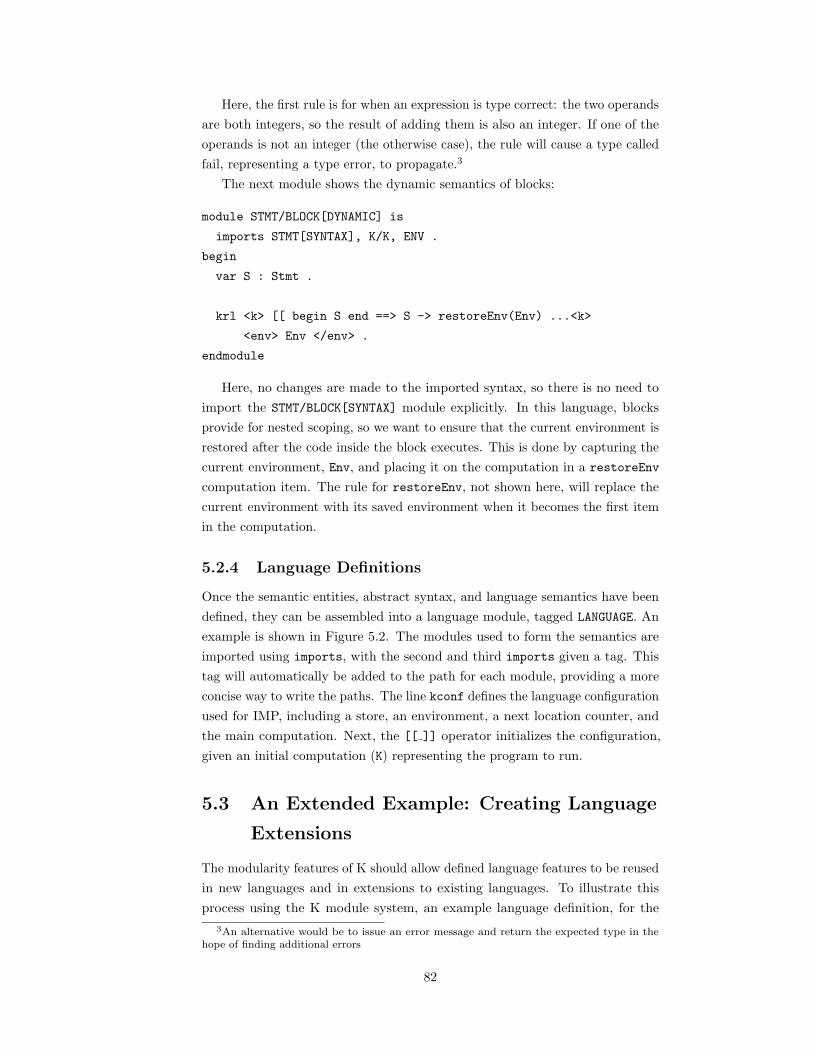
Here, the first rule is for when an expression is type correct: the two operands
are both integers, so the result of adding them is also an integer. If one of the
operands is not an integer (the otherwise case), the rule will cause a type called
fail, representing a type error, to propagate.3
The next module shows the dynamic semantics of blocks:
module STMT/BLOCK[DYNAMIC] is
imports STMT[SYNTAX], K/K, ENV .
begin
var S : Stmt .
krl <k> [[ begin S end ==> S -> restoreEnv(Env) ...<k>
<env> Env </env> .
endmodule
Here, no changes are made to the imported syntax, so there is no need to
import the STMT/BLOCK[SYNTAX] module explicitly. In this language, blocks
provide for nested scoping, so we want to ensure that the current environment is
restored after the code inside the block executes. This is done by capturing the
current environment, Env, and placing it on the computation in a restoreEnv
computation item. The rule for restoreEnv, not shown here, will replace the
current environment with its saved environment when it becomes the first item
in the computation.
5.2.4 Language Definitions
Once the semantic entities, abstract syntax, and language semantics have been
defined, they can be assembled into a language module, tagged LANGUAGE. An
example is shown in Figure 5.2. The modules used to form the semantics are
imported using imports, with the second and third imports given a tag. This
tag will automatically be added to the path for each module, providing a more
concise way to write the paths. The line kconf defines the language configuration
used for IMP, including a store, an environment, a next location counter, and
the main computation. Next, the [[ ]] operator initializes the configuration,
given an initial computation (K) representing the program to run.
5.3 An Extended Example: Creating Language
Extensions
The modularity features of K should allow defined language features to be reused
in new languages and in extensions to existing languages. To illustrate this
process using the K module system, an example language definition, for the
3An alternative would be to issue an error message and return the expected type in thehope of finding additional errors
82

module IMP[LANGUAGE]
imports K/CONFIGURATION, K/K, K/LOCATION,
VALUE, ENV, STORE, INT, BOOL .
imports[SYNTAX] EXP/AEXP/NUM, EXP/BEXP/BOOL .
imports[DYNAMIC] EXP/AEXP/NAME, EXP/AEXP/PLUS,
EXP/BEXP/LESSTHANEQ, EXP/BEXP/NOT, EXP/BEXP/AND,
STMT/SEQUENCE, STMT/ASSIGN, STMT/IFTHENELSE,
STMT/WHILE, STMT/HALT, PGM .
begin
var Store : Store .
var K : K .
var Loc : Location .
kconf <T> <store> Store </store> <env> Env </env>
<k> K </k> <nextLoc> Loc </nextLoc> </T> .
op [[_]] : K -> Configuration .
eq [[ K ]] = <T> <store> empty </store> <env> empty </env>
<k> K </k> <nextLoc> initLoc </nextLoc> .
endmodule
Figure 5.2: Language Definition: IMP
Kernel-C language [170], is shown. This is then extended to support exceptions,
providing a typical example of how a language could be extended.
5.3.1 The Kernel-C Language
A number of modules make up the definition of the abstract syntax, configuration,
and dynamic semantics for Kernel-C. These modules are discussed below.
Configurations
Kernel-C makes use of configuration items, such as Top, provided in the K
prelude. It also uses four configuration items specific to Kernel-C. The first is
the mem cell, created with a sort alias mapping sort Mem to maps from K to K (sort
K is the general sort representing computations, and includes both unevaluated
parts of the computation and computed results). Mem is used to represent the
store:
module KERNELC/CONFIG/MEM is
import K/K .
begin
sortalias Mem = KMap{K,K} .
cell mem: Mem .
endmodule
The ptr cell is defined similarly, and is used to track pointer allocation and
deallocation. Note that we could instead define a general map, KMap, from K to
K, and then define individual cells over this map. Using different sort aliases
provides a way to indicate the type of information held in the cell directly in the
cell definition.
module KERNELC/CONFIG/PTRMAP is
83

import K/K .
begin
sortalias PtrMap = KMap{K,K} .
cell ptr: PtrMap .
endmodule
Environments are also defined similarly, as maps from K to K, and provide
mappings from names in the program to memory locations:
module KERNELC/CONFIG/ENV is
import K/K .
begin
sortalias Env = KMap{K,K} .
cell env: Env .
endmodule
Finally, the out cell, representing output, is defined to just hold a single
output stream (updated with each output operation), also represented as a K:
module KERNELC/CONFIG/OUT is
import K/K .
begin
cell out: K .
endmodule
Abstract Syntax
Kernel-C includes syntax similar to the C language. Expressions, defined in
module KERNELC/EXP[SYNTAX], include generic expressions (arithmetic, boolean,
logical) from the K prelude, as well as strings:
module KERNELC/EXP[SYNTAX] is
import K/GENERIC-EXP-K-SYNTAX .
import K/STRING-K-SYNTAX .
endmodule
The DEREF syntax module defines syntax for pointer dereferencing. Note that
dereferencing is strict, since the expression indicating what is being dereferenced
should be evaluated first:
module KERNELC/EXP/MEM/DEREF[SYNTAX] is
import KERNELC/EXP[SYNTAX] .
begin
xop *_ : Exp -> Exp [strict] .
endmodule
Module MALLOC then provides syntax for the Kernel-C malloc expression,
which is similar to the malloc call found in C. malloc is also strict, with the
expression indicating the amount of storage to allocate:
module KERNELC/EXP/MEM/MALLOC[SYNTAX] is
import KERNELC/EXP[SYNTAX] .
begin
xop malloc‘(_‘) : Exp -> Exp [strict] .
endmodule
84

Also like in C, Kernel-C includes syntax for free’ing allocated memory, with
strict indicating that the expression indicating the target of the free should
be evaluated first:
module KERNELC/EXP/MEM/FREE[SYNTAX] is
import KERNELC/EXP[SYNTAX] .
begin
xop free‘(_‘) : Exp -> Exp [strict] .
endmodule
Like C, Kernel-C includes a ternary expression. The first position is strict,
since it needs to be evaluated first to determine whether to evaluate the second
or third expression next:
module KERNELC/EXP/TERNARY[SYNTAX] is
import KERNELC/EXP[SYNTAX] .
begin
xop _?_:_ : Exp Exp Exp -> Exp [strict(1)] .
endmodule
The syntax for boolean not is also renamed, this time equationally, turningit into a ternary expression. This ensures that separate semantics do not needto be given for not (hence the aux attribute):
module KERNELC/EXP/BOOL/NOT[SYNTAX] is
import KERNELC/EXP[SYNTAX] .
import KERNELC/EXP/TERNARY[SYNTAX] .
begin
var E : Exp .
xop !_ : Exp -> Exp [aux] .
eq ! E = E ? 0 : 1 .
endmodule
Assignment is defined as strict in the second argument, ensuring that the
value to assign is computed before the assignment. As will be seen later, it is
not strict in the first argument since behavior varies based on which language
construct is being assigned into:
module KERNELC/EXP/ASSIGN[SYNTAX] is
import KERNELC/EXP[SYNTAX] .
begin
xop _:=_ : Exp Exp -> Exp [strict(2)] .
endmodule
The syntax for and, like that for not, is equationally transformed to use the
ternary operator:
module KERNELC/EXP/BOOL/AND[SYNTAX] is
import KERNELC/EXP[SYNTAX] .
import KERNELC/EXP/TERNARY[SYNTAX] .
begin
vars E E’ : Exp .
xop _&&_ : Exp Exp -> Exp [aux] .
eq E && E’ = E ? E’ : 0 .
endmodule
85

The syntax for or is transformed in the same way, again allowing a semantics
to be given by translation:
module KERNELC/EXP/BOOL/OR[SYNTAX] is
import KERNELC/EXP[SYNTAX] .
import KERNELC/EXP/TERNARY[SYNTAX] .
begin
vars E E’ : Exp .
xop _||_ : Exp Exp -> Exp [aux] .
eq E || E’ = E ? 1 : E’ .
endmodule
The syntax given for printf is reminiscent of that used in C for printing
integers. Note that only one integer can be printed at a time:
module KERNELC/EXP/PRINTF[SYNTAX] is
import KERNELC/EXP[SYNTAX] .
begin
xop printf‘("%d"‘,_‘) : Exp -> Exp [strict] .
endmodule
The null keyword is introduced so that it can be used in memory operations.
Like in many C implementations, null is treated identically to 0:
module KERNELC/EXP/NULL[SYNTAX] is
import KERNELC/EXP[SYNTAX] .
begin
xop null : -> Exp [aux] .
eq null = 0 .
endmodule
After defining the syntax of expressions, the syntax for Kernel-C statements
is given. Module STMT defines both statements and lists of statements, with a
renameTo attribute indicating that lists of statements are turned into computa-
tions automatically:
module KERNELC/STMT[SYNTAX] is
begin
xsorts Stmt StmtList .
subsort Stmt < StmtList .
xop __ : StmtList StmtList -> StmtList [renameTo _->_] .
endmodule
Expressions can be made into statements by following them with a semicolon:
module KERNELC/STMT/EXPSTMT[SYNTAX] is
import KERNELC/EXP[SYNTAX] .
import KERNELC/STMT[SYNTAX] .
begin
xop _; : Exp -> Stmt [strict] .
endmodule
An empty statement, represented by just a semicolon, is also available, like in
C. It is renamed to the K identity, meaning it has the same semantics as doing
nothing:
86

module KERNELC/STMT/EMPTY[SYNTAX] is
import KERNELC/STMT[SYNTAX] .
begin
xop ; : -> Stmt [renameTo .K] .
endmodule
Two forms of blocks are provided, one with statements and an empty block.
Currently Kernel-C does not provide nested scopes, so a block is automatically
turned into a regular statement, in effect discarding the block brackets:
module KERNELC/STMT/BLOCK[SYNTAX] is
import KERNELC/STMT[SYNTAX] .
begin
xop ‘{_‘} : StmtList -> Stmt [renameTo _] .
xop ‘{‘} : -> Stmt [renameTo .K] .
endmodule
Conditionals are defined to support both one-armed and two-armed varieties.
An equation automatically converts a one-armed conditional into a two-armed
conditional with an empty block, which is why the first (one-armed) version
is marked as aux (no equations should be generated for it, since it will be
transformed anyway). The if statement is then strict in the first argument,
ensuring the guard is evaluated before a branch is selected:
module KERNELC/STMT/IF[SYNTAX] is
import KERNELC/EXP[SYNTAX] .
import KERNELC/STMT[SYNTAX] .
begin
var E : Exp . var St : Stmt .
xop if‘(_‘)_ : Exp Stmt -> Stmt [aux] .
xop if‘(_‘)_else_ : Exp Stmt Stmt -> Stmt [strict (1)] .
eq if(E) St = if (E) St else {} .
endmodule
The while loop in Kernel-C looks the same as the equivalent C construct:
module KERNELC/STMT/LOOP/WHILE[SYNTAX] is
import KERNELC/EXP[SYNTAX] .
import KERNELC/STMT[SYNTAX] .
begin
xop while‘(_‘)_ : Exp Stmt -> Stmt .
endmodule
Finally, with all the other syntax defined, it is possible to define programs.
Given in a form that looks very close to a simple C program, programs take a list
of statements. The extraneous syntax is discarded, leaving just this statement
list to execute:
module KERNELC/PGM[SYNTAX] is
import KERNELC/STMT[SYNTAX] .
begin
xsort Pgm .
xop #include<stdio.h>‘#include<stdlib.h>‘void‘main‘(void‘)‘{_‘} :
StmtList -> Pgm [renameTo _] .
endmodule
87

5.3.2 Semantics
While defining the syntax of Kernel-C a number of constructs where transformed
into other constructs, using either the renameTo attribute or using equations.
Because of this, fewer semantic definitions are needed, with one definition often
providing semantics for multiple (syntax-level) language features. Some semantic
definitions are also given in the K prelude – these are brought in in module
KERNELC/EXP[DYNAMIC] by importing module K/GENERIC-EXP-SEMANTICS:
module KERNELC/EXP[DYNAMIC] is
import K/GENERIC-EXP-SEMANTICS .
endmodule
The semantics for booleans automatically transforms them into numbers,
similar to the semantics for operations that work with “booleans” in C (booleans
in quotes, because C has no real booleans):
module KERNELC/EXP/BOOL[DYNAMIC] is
import KERNELC/EXP[DYNAMIC] .
begin
eq #(true) = #(1) .
eq #(false) = #(0) .
endmodule
The semantics for dereferencing use several K constructs. The context
definition enforces strictness in assignment for the first operand when it is a
dereferencing operation; the two keq definitions then give the semantics both
for a lookup through a pointer and an assignment through a pointer:
module KERNELC/EXP/MEM/DEREF[DYNAMIC] is
import KERNELC/EXP[DYNAMIC] .
import KERNELC/CONFIG/MEM .
import KCONFIG/CONFIG .
begin
vars K1 K2 : K .
var N : Nat .
vars V V’ : KResult .
kcxt * K1 := K2 [strict(K1)] .
krl <k> [[* #(N) ==> V]] ...</k>
<mem>... #(N) |-> V ...</mem> .
krl <k> [[* #(N) := V ==> V]] ...</k>
<mem>... #(N) |-> [[V’ ==> V]] ...</mem> .
endmodule
The malloc semantics handle memory allocation, returning the new memory
location and performing the proper bookkeeping in the pointer map stored in cell
ptr. Note the use of K/FRESH-ITEM{K} below: this is a parameterized module
from the K prelude (hence the prefix of K/), with the parameter the sort K:
module KERNELC/EXP/MEM/MALLOC[DYNAMIC] is
88

import KERNELC/EXP[DYNAMIC] .
import KERNELC/CONFIG/MEM .
import KERNELC/CONFIG/PTRMAP .
import KCONFIG/CONFIG .
import K/FRESH-ITEM{K} .
begin
vars N N’ : Nat . var NV : NatVar .
op alloc : Nat Nat -> PtrMap .
eq alloc(N, 0) = .empty .
eq alloc(N, s(N’)) = (#(N) |-> #(0)) &’ alloc(N + 1, N’) .
krl <k> [[ malloc(#(N)) ==> #(N’)]] ...</k>
<ptr>... [[.empty ==> (#(N’) |-> #(N))]] ...</ptr>
<nextItem> [[item(N’) ==> item(N’) + N]] </nextItem>
<mem>... [[.empty ==> alloc(N’, N)]] ...</mem> .
endmodule
Using free does the opposite, using this earlier bookkeeping information to
properly clean up allocated storage:
module KERNELC/EXP/MEM/FREE[DYNAMIC] is
import KERNELC/EXP[DYNAMIC] .
import KCONFIG/CONFIG .
import KERNELC/CONFIG/MEM .
import KERNELC/CONFIG/PTRMAP .
begin
vars N N’ : Nat .
var V : KResult .
var Mem : Mem .
op void : -> KResult .
op freeMem : PtrMap Nat Nat -> PtrMap .
eq freeMem(Mem, N, 0) = Mem .
eq freeMem((Mem &’ (#(N) |-> V)), N, s(N’)) = freeMem(Mem,N + 1,N’) .
krl <k> [[free(#(N)) ==> void]] ...</k>
<ptr>... [[#(N) |-> #(N’) ==> .empty]] ...</ptr>
<mem> [[Mem ==> freeMem(Mem, N, N’)]] </mem> .
endmodule
The ternary expression works the same as in C. The first expression is
evaluated to a numeric value. If this value is not 0, it represents the true case,
and the second expression is evaluated. If this value is 0, it represents the false
case, and the third expression is evaluated:
module KERNELC/EXP/TERNARY[DYNAMIC] is
import KERNELC/EXP[DYNAMIC] .
begin
vars K1 K2 : K .
var I : Int .
eq (#(0)) ? K1 : K2 = K2 .
ceq (#(I)) ? K1 : K2 = K1 if I neq 0 .
endmodule
89

Assignment works as expected; since this assignment does not involve deref-
erencing, the value can be stored directly in the environment, with storage to
memory limited to those cases where the value can be updated through a pointer:
module KERNELC/EXP/ASSIGN[DYNAMIC] is
import KERNELC/EXP[DYNAMIC] .
import KERNELC/CONFIG/ENV .
import KCONFIG/CONFIG .
begin
var X : Name .
var V : KResult .
var Env : Env .
krl <k> [[X := V ==> V]] ...</k>
<env> [[Env ==> Env[X <- V]]] </env> .
endmodule
Non-pointer lookups retrieve the value stored in the environment using
assignment:
module KERNELC/EXP/LOOKUP[DYNAMIC] is
import KERNELC/EXP[DYNAMIC] .
import KERNELC/CONFIG/ENV .
import KCONFIG/CONFIG .
begin
var X : Name .
var V : KResult .
krl <k> [[X ==> V]] ...</k>
<env>... X |-> V ...</env> .
endmodule
The printf expression uses the given value to update the contents of the
stream stored in cell out:
module KERNELC/EXP/PRINTF[DYNAMIC] is
import KERNELC/EXP[DYNAMIC] .
import KCONFIG/CONFIG .
import KERNELC/CONFIG/OUT .
begin
var I : Int .
var S : String .
op stream : String -> K .
krl <k> [[printf("%d",#(I)) ==> void]] ...</k>
<out> [[stream(S) ==> stream(S + string(I,10)+ " ")]] </out> .
endmodule
The base semantics for statements import the base expression semantics,
which they rely on:
module KERNELC/STMT[DYNAMIC] is
import KERNELC/EXP[DYNAMIC] .
endmodule
90

Expression statements can then be treated essentially as no-ops, once the
expression is evaluated (which is automatic because of the strictness annotation
on the ; operator). The value is not used, so it is just discarded:
module KERNELC/STMT/EXPSTMT[DYNAMIC] is
import KERNELC/STMT[DYNAMIC] .
begin
var V : KResult .
eq V ; = .K .
endmodule
The if semantics also rely on strictness, with one rule each for the situation
where the condition is false (i.e., 0) and where the condition is true (i.e., not 0):
module KERNELC/STMT/IF[DYNAMIC] is
import KERNELC/STMT[DYNAMIC] .
begin
vars K1 K2 : K .
var I : Int .
eq if (#(0)) K1 else K2 = K2 .
ceq if (#(I)) K1 else K2 = K1 if I neq 0 .
endmodule
While loops are given a semantics in a standard way, with a translation into
an equivalent conditional that first checks the while guard and then, if true,
executes the body and then schedules the loop for another iteration:
module KERNELC/STMT/LOOP/WHILE[DYNAMIC] is
import KERNELC/STMT[DYNAMIC] .
import KERNELC/STMT/IF[DYNAMIC] .
begin
vars K1 K2 : K .
keq <k> [[while (K1) K2 ==> if (K1) (K2 -> while(K1) K2) else .K]] ...</k> .
endmodule
5.3.3 Language Definition
Using the already-defined modules, the language can be constructed. Dynamic
semantics modules are imported, as well as syntax modules that are not imported
by the dynamic semantics (remember, syntax modules are automatically imported
into other modules with the same name, sans tag). The configuration is then
created – it is not really needed here, since all cells are at the same level, but
will come in handy later, and also provides good documentation. Finally, a run
operation is provided, which, given an initial computation, will correctly set up
the configuration so program execution can start:
module KERNELC/STANDARD[LANGUAGE] is
import[DYNAMIC]
91

KERNELC/EXP/BOOL, KERNELC/EXP/MEM/DEREF, KERNELC/EXP/MEM/MALLOC,
KERNELC/EXP/MEM/FREE, KERNELC/EXP/TERNARY, KERNELC/EXP/ASSIGN,
KERNELC/EXP/LOOKUP, KERNELC/EXP/PRINTF, KERNELC/STMT/EXPSTMT,
KERNELC/STMT/IF, KERNELC/STMT/LOOP/WHILE .
import[SYNTAX]
KERNELC/EXP/TERNARY, KERNELC/EXP/BOOL/NOT, KERNELC/EXP/BOOL/AND,
KERNELC/EXP/BOOL/OR, KERNELC/EXP/NULL, KERNELC/STMT/EMPTY,
KERNELC/STMT/BLOCK, KERNELC/PGM .
begin
var P : Pgm .
var K : K .
var Env : Env .
var Mem : Mem .
var Ptr : PtrMap .
var I : Item .
var S : K .
kconf <T> <k> K </k> <env> Env </env> <mem> Mem </mem>
<ptr> Ptr </ptr> <nextItem> I </nextItem>
<out> S </out> </T> .
op run : Pgm -> Config .
eq run(P)
= <T>
<k> mkK(P) </k> <env> .empty </env>
<mem> .empty </mem> <ptr> .empty </ptr>
<nextItem> item(1) </nextItem>
<out> stream("") </out>
</T> .
endmodule
5.3.4 Adding Exceptions to Kernel-C
The exceptions extension to Kernel-C provides a simple exceptions mechanism,
with a try/catch block similar to that used in Java and a throw statement
that triggers an exception. The first step to adding exceptions is to define the
configuration needed for exceptions, as well as some operators that work with
the exception state:
module KERNELC/CONFIG/EXCEPTIONS is
import KERNELC/CONFIG/ENV .
import K/K .
begin
sortalias ExStack = KList{K} .
cell es : ExStack .
vars K K’ : K .
var ES : ExStack .
op removeHandler : -> K .
krl <k> [[ removeHandler ==> .K ]] ...</k>
<es> [[ K, ES ==> ES ]] </es> .
92

op addHandler : K -> K .
krl <k> [[ addHandler(K) ==> .K ]] ...</k>
<es> [[ ES ==> K, ES ]] </es> .
op handleException : -> K .
krl <k> [[ handleException -> K’ ==> K ]] </k>
<es> [[ K, ES ==> ES ]] </es> .
endmodule
A new sort alias, ExStack, is declared. An exception stack is a list of
computations (Ks) treated as a stack. A new cell, es, is also defined; this cell will
be used in the semantics to hold the stack. Using this new sort alias and cell,
three operators are then defined, along with semantic equations. removeHandler
is used to remove the top exception handler from the stack without actually
triggering the handler; handleException does the same, but it does trigger
the exception handler, replacing the current computation (K’) with the handler
computation. addHandler adds the handler onto the stack.
It is now possible to define the syntax and semantics for exceptions. The
syntax for try/catch provides two statements: the code being handled, and the
handler for when exceptions are thrown. try/catch is itself also a statement:
module KERNELC/STMT/TRYCATCH[SYNTAX] is
import KERNELC/STMT[SYNTAX] .
begin
xop try_catch_; : Stmt Stmt -> Stmt .
endmodule
The semantics use the addHandler and removeHandler operators defined
above. When a try/catch block is encountered, the semantics are defined to
add a handler to the stack. This handler will run the computation in the catch
block and will then pick up with whatever computation is after the try/catch
construct. The code inside the try is then run after the handler is added. After
this, the removeHandler item will remove the added handler; this will only be
run if the handler is not triggered by an exception.
module KERNELC/STMT/TRYCATCH[DYNAMIC] is
import KERNELC/STMT[DYNAMIC] .
import KERNELC/CONFIG/EXCEPTIONS .
begin
vars K K’ K’’ : K .
krl <k> [[ try K catch K’ ; ==>
addHandler(K’ -> K’’) -> K -> removeHandler ]]
-> K’’ </k>
endmodule
The syntax for throw defines it as a statement. Unlike in Java, it does not
actually throw a value, so it is not given an expression to evaluate:
module KERNELC/STMT/THROW[SYNTAX] is
import KERNELC/STMT[SYNTAX] .
93

begin
xop throw; : -> Stmt .
endmodule
Finally, semantics are given to throw. A throw will trigger the exception
handler using the handleException item:
module KERNELC/STMT/THROW[DYNAMIC] is
import KERNELC/STMT[DYNAMIC] .
import KERNELC/CONFIG/EXCEPTIONS .
begin
krl <k> [[ throw; ==> handleException ]] ... </k>
endmodule
The new features are added by creating a new language version with imports
for the new modules. Note that none of the old modules needed to change. Here
we add the exception stack to the configuration, and we also add an additional
level of grouping, with the k and es cells added under another cell, control
(which we assume, for this example, is imported from the prelude, but could
easily be added manually). The use of context transformers allows the existing
rules that use k and other cells to continue to function unchanged.
module KERNELC/WEXCEPTIONS[LANGUAGE] is
import[DYNAMIC]
KERNELC/EXP/BOOL, KERNELC/EXP/MEM/DEREF, KERNELC/EXP/MEM/MALLOC,
KERNELC/EXP/MEM/FREE, KERNELC/EXP/TERNARY, KERNELC/EXP/ASSIGN,
KERNELC/EXP/LOOKUP, KERNELC/EXP/PRINTF, KERNELC/STMT/EXPSTMT,
KERNELC/STMT/IF, KERNELC/STMT/LOOP/WHILE, KERNELC/STMT/TRYCATCH,
KERNELC/STMT/THROW .
import[SYNTAX]
KERNELC/EXP/TERNARY, KERNELC/EXP/BOOL/NOT, KERNELC/EXP/BOOL/AND,
KERNELC/EXP/BOOL/OR, KERNELC/EXP/NULL, KERNELC/STMT/EMPTY,
KERNELC/STMT/BLOCK, KERNELC/PGM .
begin
var P : Pgm .
var K : K .
var Env : Env .
var Mem : Mem .
var Ptr : PtrMap .
var I : Item .
var S : K .
var ES : ExStack .
kconf <T> <ctrl> <k> K </k> <es> ES </es> </control>
<env> Env </env> <mem> Mem </mem>
<ptr> Ptr </ptr> <nextItem> I </nextItem>
<out> S </out> </T> .
op run : Pgm -> Config .
eq run(P)
= <T>
<control> <k> mkK(P) </k> <es> .empty </es> </control>
<env> .empty </env> <mem> .empty </mem>
<ptr> .empty </ptr> <nextItem> item(1) </nextItem>
94
<out> stream("") </out>
</T> .
endmodule
5.4 Translating K Modules to Maude
K module definitions are translated into a K Maude format supported by the
current release of the K tools, which is then translated to Maude. This section
focused on the first part of this translation; the second is part of ongoing work,
but is not part of the work on the module system. The K Maude format used
in the K tools is not modular, allowing either one module, with the entire
language definition, or three, one for syntax, one for the configuration, and one
for semantics. Because of this, one of the main tasks of the translation is to
“flatten” the information given in the K modules into a non-modular form.
Standard Features: Many of the constructs in the module system are already
valid in the K tools format, and require no translation. This includes subsorts
and operator definitions. Other constructs have very lightweight translations:
syntax ops are translated into regular ops with the same names, signatures, etc.
One current limitation of the module system tools support is that, because the
parsing is currently deferred until the K tools form of the semantics is presented
to Maude, several features that rely on parsing are not yet fully supported. This
includes altering of attributes on imports, some renamings, and some uses of
exports and requires.
Features Requiring Significant Translation: The remaining features are
handled as follows:
• Each sort is defined in its own module, with that module then imported into
the module that initially defined the sort. A view is created automatically
for each sort from TRIV to the sort module, mapping Elt to the sort.
• Each sort alias is defined in its own module, using import renamings to
map the original name for the sort (e.g., Map{K,K}) to the alias name (e.g.,
Mem).
• Syntax sorts, syntax operators, and subsorts using the syntax sorts are all
generated into the syntax module: the sorts are added to the module as
imports, while the operators and subsorts are added as actual operator
and subsort definitions.
• Cells are translated into operators in the configuration module, with a
special attribute on each operator describing the cell contents.
• Other items are translated into a single semantics module. Variables and
variable prefixes are used to decorate variables in rules and equations with
95
sort information, and are not otherwise included in the final generated
module. Variable prefixes are used based on reachability, to ensure that
only imported (directly or indirectly) prefixes can be used. Configurations
and contexts (with variable sort decoration) are also brought over directly.
Semantic sorts and sort aliases are handled identically to syntax sorts and
sort aliases.
Module Headers: Exports clauses that do not mention syntax items (the
standard case – generally one does not hide abstract syntax, but instead hides
special operators or sorts used inside other modules) are modeled by moving the
module contents to a second module. The original module then imports this
second module, renaming all private operators, sorts, and cells. This does not
prevent use of these private constructs, but protects against inadvertent use or
duplication, which is the goal of the exports feature.
Imports are converted directly into Maude-style including directives, with
any special prefixes (e.g., the K on K/INT-SYNTAX) removed first. These import
paths are collected based on which modules are reachable, ensuring all needed
imports are given in the proper three modules while not either importing modules
that have been translated away or that only contain information used by another
of the three modules (e.g., the syntax does not import all the semantics).
5.5 The Online Semantics Repository
One goal of the K module system is to allow modules to easily be shared and
reused. To help support this goal an online repository of semantics modules
is being developed. At this point, a basic version of the repository, targeted
specifically at K modules, has been developed. It is expected that further work
on this repository will include closer tool integration and the ability to support
additional module formats, such as standard rewriting logic semantics modules
and MSOS modules.
5.5.1 The Repository Backend
The repository currently uses a database to store information about each module.
Each module record is assigned a unique identifier, and also contains information
such as: module name; module version; a description of the module; when the
module was last updated, and by whom; the type of semantics inside the module;
the modules required for this module to work properly; and the features defined
by this module. The current main purpose of the backend is to store and provide
data for the module exchange format, described below, but in the future tools
may directly access the database to work with the modules in the repository.
96

5.5.2 An XML Format for Module Exchange
To enable the exchange of semantic modules between K tool support and the
module repository, and with an eye towards future interfacing with other tools
or other module formats, an initial definition of a shared format for exchanging
semantic modules has been defined. The XML Schema definition for this format
can be found in Figure 5.3.
An XML document containing a semantic module definition is made up of
the overall definition, a list of other required modules, and a list of features
provided by this module. Figure 5.4 focuses on the overall definition. It includes
the module name, a module namespace, providing a way to group modules by
provider, and a version number for the module. Also included are several fields
indicating when the module was last modified (lastModifiedOn), and by whom
(lastModifiedBy); the type of semantics (semanticsType), such as K or MSOS;
and a description of the module.
The requirements of the module, currently in field requirements, are given
in terms of required modules. Each required module is of type RequiredModule,
the definition of which is given in Figure 5.5. The information for the module
requirement includes a path, which is made up of the namespace followed by the
module name, and a required version. Currently the required version must be
an exact match; a possible future modification is to allow additional information,
either with version numbering patterns or comparison operations (ranges, version
greater than the given number, etc).
Individual features, of type Feature, are given inside the features tag. The
format for features is shown in Figure 5.6. A feature description is made up of a
feature name, a feature description, a numeric feature type, and the feature
contents. The meaning of these fields is dependent on the style of semantics.
In K, the name and description provide optional descriptive information, the
contents is the actual K text, and the type indicates the type of feature being
given, with different numbers for syntactic operators, k rules, etc.
Figure 5.7 provides an example of a module that defines both the abstract
syntax and semantics for addition. The name of the module is Exp/AExp/Plus,
and it is part of namespace FSL. The version number is set to 1.0, and the
semantics type to K. Two modules are listed as requirements, both in the FSL
namespace, and both at version 1.0 as well. Also, two features are defined. The
first is a syntax operator, the second a K rule for addition. The name and
description are arbitrary, while the types indicate the type of feature (6 is a
syntax operator, 14 a K rule).
5.5.3 Client-Side Tool Support
Client-side tool support is based around a command line tool that communi-
cates with the repository using web services. Currently, several operations are
supported:
97
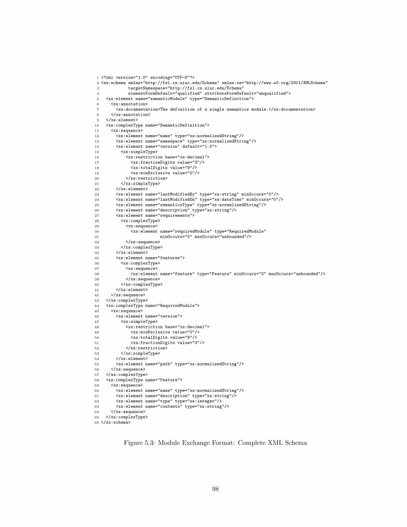
1 <?xml version="1.0" encoding="UTF-8"?>2 <xs:schema xmlns="http://fsl.cs.uiuc.edu/Schema" xmlns:xs="http://www.w3.org/2001/XMLSchema"3 targetNamespace="http://fsl.cs.uiuc.edu/Schema"4 elementFormDefault="qualified" attributeFormDefault="unqualified">5 <xs:element name="semanticModule" type="SemanticDefinition">6 <xs:annotation>7 <xs:documentation>The definition of a single semantics module.</xs:documentation>8 </xs:annotation>9 </xs:element>
10 <xs:complexType name="SemanticDefinition">11 <xs:sequence>12 <xs:element name="name" type="xs:normalizedString"/>13 <xs:element name="namespace" type="xs:normalizedString"/>14 <xs:element name="version" default="1.0">15 <xs:simpleType>16 <xs:restriction base="xs:decimal">17 <xs:fractionDigits value="3"/>18 <xs:totalDigits value="9"/>19 <xs:minExclusive value="0"/>20 </xs:restriction>21 </xs:simpleType>22 </xs:element>23 <xs:element name="lastModifiedBy" type="xs:string" minOccurs="0"/>24 <xs:element name="lastModifiedOn" type="xs:dateTime" minOccurs="0"/>25 <xs:element name="semanticsType" type="xs:normalizedString"/>26 <xs:element name="description" type="xs:string"/>27 <xs:element name="requirements">28 <xs:complexType>29 <xs:sequence>30 <xs:element name="requiredModule" type="RequiredModule"31 minOccurs="0" maxOccurs="unbounded"/>32 </xs:sequence>33 </xs:complexType>34 </xs:element>35 <xs:element name="features">36 <xs:complexType>37 <xs:sequence>38 <xs:element name="feature" type="Feature" minOccurs="0" maxOccurs="unbounded"/>39 </xs:sequence>40 </xs:complexType>41 </xs:element>42 </xs:sequence>43 </xs:complexType>44 <xs:complexType name="RequiredModule">45 <xs:sequence>46 <xs:element name="version">47 <xs:simpleType>48 <xs:restriction base="xs:decimal">49 <xs:minExclusive value="0"/>50 <xs:totalDigits value="9"/>51 <xs:fractionDigits value="3"/>52 </xs:restriction>53 </xs:simpleType>54 </xs:element>55 <xs:element name="path" type="xs:normalizedString"/>56 </xs:sequence>57 </xs:complexType>58 <xs:complexType name="Feature">59 <xs:sequence>60 <xs:element name="name" type="xs:normalizedString"/>61 <xs:element name="description" type="xs:string"/>62 <xs:element name="type" type="xs:integer"/>63 <xs:element name="contents" type="xs:string"/>64 </xs:sequence>65 </xs:complexType>66 </xs:schema>
Figure 5.3: Module Exchange Format: Complete XML Schema
98
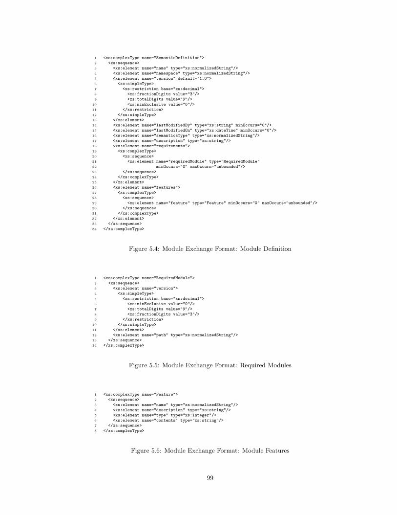
1 <xs:complexType name="SemanticDefinition">2 <xs:sequence>3 <xs:element name="name" type="xs:normalizedString"/>4 <xs:element name="namespace" type="xs:normalizedString"/>5 <xs:element name="version" default="1.0">6 <xs:simpleType>7 <xs:restriction base="xs:decimal">8 <xs:fractionDigits value="3"/>9 <xs:totalDigits value="9"/>
10 <xs:minExclusive value="0"/>11 </xs:restriction>12 </xs:simpleType>13 </xs:element>14 <xs:element name="lastModifiedBy" type="xs:string" minOccurs="0"/>15 <xs:element name="lastModifiedOn" type="xs:dateTime" minOccurs="0"/>16 <xs:element name="semanticsType" type="xs:normalizedString"/>17 <xs:element name="description" type="xs:string"/>18 <xs:element name="requirements">19 <xs:complexType>20 <xs:sequence>21 <xs:element name="requiredModule" type="RequiredModule"22 minOccurs="0" maxOccurs="unbounded"/>23 </xs:sequence>24 </xs:complexType>25 </xs:element>26 <xs:element name="features">27 <xs:complexType>28 <xs:sequence>29 <xs:element name="feature" type="Feature" minOccurs="0" maxOccurs="unbounded"/>30 </xs:sequence>31 </xs:complexType>32 </xs:element>33 </xs:sequence>34 </xs:complexType>
Figure 5.4: Module Exchange Format: Module Definition
1 <xs:complexType name="RequiredModule">2 <xs:sequence>3 <xs:element name="version">4 <xs:simpleType>5 <xs:restriction base="xs:decimal">6 <xs:minExclusive value="0"/>7 <xs:totalDigits value="9"/>8 <xs:fractionDigits value="3"/>9 </xs:restriction>
10 </xs:simpleType>11 </xs:element>12 <xs:element name="path" type="xs:normalizedString"/>13 </xs:sequence>14 </xs:complexType>
Figure 5.5: Module Exchange Format: Required Modules
1 <xs:complexType name="Feature">2 <xs:sequence>3 <xs:element name="name" type="xs:normalizedString"/>4 <xs:element name="description" type="xs:string"/>5 <xs:element name="type" type="xs:integer"/>6 <xs:element name="contents" type="xs:string"/>7 </xs:sequence>8 </xs:complexType>
Figure 5.6: Module Exchange Format: Module Features
99

• retrieve a list of the modules contained in the repository;
• retrieve a specific module from the repository;
• retrieve a specific module from the repository, including all modules tran-
sitively required by the module.
Modules are currently inserted by generating SQL directly from the modtool
command-line interface to the module system, which is also used to perform
translations from modules in the module system into the Maude K tool format.
One future task is to make the repository open for outside updates, which will
require proper security support to ensure that only authorized users can modify
repository contents.
5.6 Discussion
Chapters 3, 4, and 5 presented methods and tools for the modular definition of
language features, including (in this chapter) a module system to allow the reuse
of these features. This section discusses some of the limitations of this work; a
comparison with other related work is provided in Chapter 9.
First, some language features seem to be inherently non-modular. While it is
possible to define these features using K, it may still be necessary to either alter
one or more imported modules (not recommended) or create new versions of
1 <?xml version="1.0" encoding="UTF-8"?>2 <semanticModule xmlns="http://fsl.cs.uiuc.edu/Schema"3 xmlns:xsi="http://www.w3.org/2001/XMLSchema-instance"4 xsi:schemaLocation="http://fsl.cs.uiuc.edu/Schema/Semantics.xsd">5 <name>Exp/AExp/Plus</name>6 <namespace>FSL</namespace>7 <version>1.0</version>8 <semanticsType>K</semanticsType>9 <description>Syntax and semantics of integer addition.</description>
10 <requirements>11 <requiredModule>12 <version>1.0</version>13 <path>FSL::K/Builtins/Data/Integer</path>14 </requiredModule>15 <requiredModule>16 <version>1.0</version>17 <path>FSL::K/Builtins/Configs/K</path>18 </requiredModule>19 </requirements>20 <features>21 <feature>22 <name>Syntax</name>23 <description>Abstract syntax for plus.</description>24 <type>6</type>25 <contents>xop _+_ : AExp AExp -> AExp [strict] .</contents>26 </feature>27 <feature>28 <name>Semantics</name>29 <description>Dynamic semantics for plus.</description>30 <type>14</type>31 <contents>krl <k> [[ I1 + I2 ==> int+(I1,I2) ]]...</k> .</contents>32 </feature>33 </features>34 </semanticModule>
Figure 5.7: Module Exchange Format: Example Module
100

some modules that are specific to the feature being defined. One example of this,
presented in Chapter 3, was synchronized methods. Because locks need to be
properly tracked at method entry and exit, defining synchronized methods also
required changing the definition of exceptions, ensuring that any locks acquired
on entry to a synchronized method are released as the stack frame is unrolled.
Another example would be a Java-like finally clause on an exception handler,
which impacts the semantics of method return and loop break and continue as
well. For instance, if an exception handler is provided in the body of a loop, a
break statement given inside the try block would trigger the finally clause.
In both of these cases, this means the semantics of other features need to change
when the new feature is introduced.
Second, while the K module system is quite flexible, the downside of this is
that the module system does not provide support for good definitional style. In
other words, it allows one to write modules that are not in fact modular, packing
a number of features into a single module. While we believe that this is essential,
to allow the user the freedom to define modules in a style with which the user is
comfortable, it would be useful to allow the enforcement of good style in cases
where the intent is to later share the modules with others.
Third, the support in the K module system of Maude attributes, such as the
format and prec attributes, can tie K modules defined using the module system
closely to Maude. For instance, the prec attribute could be added to the DEREF
abstract syntax shown above to allow for the proper parsing of programs given
as Maude terms:
module KERNELC/EXP/MEM/DEREF[SYNTAX] is
import KERNELC/EXP[SYNTAX] .
begin
xop *_ : Exp -> Exp [strict prec 25] .
endmodule
Or, the format attribute could be used in the abstract syntax for MALLOC to
provide proper formatting (spacing, newlines, colors, etc) of the operator when
it is output in Maude:
module KERNELC/EXP/MEM/MALLOC[SYNTAX] is
import KERNELC/EXP[SYNTAX] .
begin
xop malloc‘(_‘) : Exp -> Exp [format (g b o b o) strict] .
endmodule
Since it is not required that one use these attributes, it is still possible to
write modules for features which can then be reused in different languages (for
instance, languages where the precedence is different). However, it is currently
necessary to use these attributes if one wishes to provide programs directly as
Maude terms, instead of writing a language front-end which will generate an
abstract syntax for the program in a Maude-friendly form (such as is done in both
KOOL and Beta). One possible solution is to add a layer in the transformation
101

from K modules to a target platform, such as Maude, that allows transformations
– the addition of attributes, etc – to be performed on the individual items in a
module body.
102

Chapter 6
Language Design and
Performance
Many methods of defining languages are based solely on paper definitions,
potentially with tool support to help properly typeset rules in the semantics.
For such formalisms performance is not even a consideration. However with
executable specifications, performance can be critical, especially when using the
definitions in practical situations, such as during language prototyping or program
analysis. This chapter discusses research on improving the performance of K
definitions implemented using Maude. Section 6.1 focuses mainly on execution
performance, illustrating how changes in the memory representations used by
language definitions can speed up certain programs. Section 6.2 then shifts this
focus to analysis performance, showing how changes to the KOOL language,
discussed in Chapter 3, can both make analysis faster and allow larger programs
to be analyzed. This chapter serves as a bridge between the earlier chapters,
which have focused on language semantics, and the later chapters, which focus
more directly on program analysis.
The definitions of syntax and semantics in this chapter are shown using
Maude syntax, instead of directly in K syntax. All equations and rules use the
K definitional style in Maude.
6.1 Execution Performance
Because of the executability of the semantic rules used in K definitions, changes
to the definitions of language features and the semantic configuration can have
a large impact on performance. One temptation is to modify features in the
language directly, trying a number of permutations to determine which perform
best. While this may be acceptable in certain circumstances, in other cases it
may lead to definitions of language features that either no longer really define the
feature correctly (for instance, by restricting behavior to improve performance,
at the cost of eliminating behaviors allowed by the language) or are too complex,
sacrificing simplicity and understandability for speed.
One promising direction is to change, not the rules defining the semantics of
language features, but those defining the surrounding configuration. Since the
configuration is seen as an abstraction inside the language rules, changes to the
configuration can occur without requiring changes to the semantics of language
103

Integer Numbers N ::= (+|-)?(0..9)+
Declarations D ::= var I | var I[N ]
Expressions E ::= N | E + E | E - E | E * E | E / E | E % E | - E |
E < E | E <= E | E > E | E >= E | E = E | E != E |
E and E | E or E | not E | N | I(El) | I[E] | I | read
Expression Lists El ::= E (, E)∗
| nil
Statements S ::= I := E | I[E] := E | if E then S fi | if E then S else S fi |
for I := E to E do S od | while E do S od | S; S | D |
I(El) | return E | write E
Function Declarations FD ::= function I(Il) begin S end
Identifiers I ::= (a− zA− Z)(a− zA− Z0− 9)∗
Identifier Lists Il ::= I (, I)∗
| void
Programs Pgm ::= S? FD+
Figure 6.1: Syntax for SILF
constructs. Beyond this, configurations are often reused between languages,
allowing improvements to be directly leveraged inside other definitions. This
section describes changes to two languages, SILF [86] and KOOL, both at the
level of the memory representation in the configuration. Section 6.1.1 shows the
first memory representation change, introducing a stacked memory model to
SILF; performance comparisons show the benefit of this model, while comparisons
with the prior version show that few changes to the semantics are needed. After
this, Section 6.1.2 shows the second change, the addition of a basic mark-sweep
garbage collector to KOOL, including discussions of performance and reusability.
6.1.1 SILF and Stacked Memory
SILF, the Simple Imperative Language with Functions, is a basic imperative
language with many core imperative features: functions, global variables, loops,
conditionals, and arrays. Programs are made up of a series of variable and
function declarations, with a designated function named main serving as the
entry point to the program. The syntax of SILF is shown in Figure 6.1, while a
sample program, which computes the factorial of 200 recursively, is shown in
function factorial(n)
begin
if n = 0 then
return 1
else
return n * factorial(n - 1)
fi
end
function main(void)
begin
write factorial(200)
end
Figure 6.2: Recursive Factorial, SILF
104

Figure 6.2.
The SILF Memory Model
In SILF, memory is allocated automatically for global and local variables and
arrays, including for the formal parameters used in function calls. Users are not
able to allocate additional storage with operations like new or function calls like
C’s malloc, and are not able to create pointers/references or capture variable
addresses. SILF includes a simple memory model, where memory is represented
as a set of Location × Value pairs, referred to as StoreCells; the entire set
is just called the Store 1. This, or something very similar, is the standard
model used in a number of languages defined using K or the computation-based
definitional style2:
sorts StoreCell Store .
subsort StoreCell < Store .
op [_,_] : Location Value -> StoreCell .
op nil : -> Store .
op __ : Store Store -> Store [assoc comm id: nil] .
The main advantage of this model is that memory operations are simple to
define; memory update and lookup can be performed just using matching within
the Store, as shown here for variable lookup:
eq k(exp(X) -> K) env(Env [X,L])
= k(lookupLoc(L) -> K) env(Env [X,L]) .
eq k(lookupLoc(L) -> K) store(Mem [L,V])
= k(val(V) -> K) store(Mem [L,V]) .
Here, exp(X) means there is an expression X, a variable name; matching
is used to find the location of X, L, in the current environment, a set of Name
× Location pairs. This triggers the lookup of location L using operation
lookupLoc. When this operation is processed, matching is performed against
the store, returning the value V stored at location L.
This model has a major disadvantage, though: old locations are never
removed from the store, even when they become unreachable, which happens
quite often (formals become unreachable after each function return, for instance).
As memory grows, it takes longer to match against the store, slowing execution
performance.
1In SILF, a StoreCell is actually called a <Location><Value>, which has an associated<Location><Value>Set representing the Store. The terminology is changed here to make itsimpler to read and type.
2Newer definitions often use the built-in MAP module instead; this is used by KOOL, forinstance, as described in Section 6.1.2.
105

Stacked Memories
As mentioned above, it is not possible in SILF to dynamically allocate memory or
take the addresses of variables. This prevents addresses from escaping a function,
since there is no way to return a pointer to something inside the function; because
of this, it should be possible to discard all memory allocated for the function call
when the function returns3. A conceptually simple way to do this is to change
from a flat memory to a stack of memories, with the memory for the current
function on top and the global memory on the bottom. Memories can still be
treated as sets of StoreCells, but each set can be much smaller, containing just
the cells allocated in the current function, and each set can easily be discarded
simply by popping the stack at function return. Following this reasoning, the
memory model for SILF can be changed appropriately:
sort StackFrame Stack .
subsort StackFrame < Stack .
op [_,_] : Nat Store -> StackFrame .
op nil : -> Stack .
op _,_ : Stack Stack -> Stack [assoc id: nil] .
Here, each element of the stack is referred to by the name StackFrame, a fa-
miliar term meant to show the intuition behind the technique. Each StackFrame
is actually a pair, a Store and a natural number representing the first location
in the frame; attempts to access a lower numbered location need to check in
earlier frames, here the bottom frame, since SILF’s scoping only allows access to
local or global names and does not allow nested functions. These StackFrames
are assembled into Stacks, with the head of the list as the top element of the
stack and the last element of the list the global frame.
Location lookup is now slightly more involved:
op stackLookup : Location Stack -> Value .
op lvsLookup : Location Store -> Value .
eq k(lookupLoc(L) -> K) store(ST)
= k(val(stackLookup(L,ST)) -> K) store(ST) .
ceq stackLookup(loc(N),([Nb,Mem], ST))
= lvsLookup(loc(N),Mem)
if N >= Nb .
ceq stackLookup(loc(N),([Nb,Mem], ST, [Nb’,Mem’]))
= lvsLookup(loc(N),Mem’)
if N < Nb .
eq lvsLookup(L,([L,V] Mem)) = V .
3This seems restrictive, but is actually standard for stack-allocated memory in imperativeor object-oriented languages without address capture, such as Java or Pascal. Heap-allocatedmemory could not be similarly discarded.
106

Standard (Flat) Memory Model Stacked Memory ModelTest Case Time (sec) Time (sec)factorial 3.711 0.747factorial2 1664.280 11.245ifactorial 1.047 0.978ifactorial2 43.861 15.441fibonacci 29.014 1.939
qsort 111.623 15.374ssort 21.557 14.657
Single 3.40 GHz Pentium 4, 2 GB RAM, OpenSuSE 10.2, kernel 2.6.18.8-0.7-default, Maude 2.3.
Times and rewrites per second averaged over three runs of each test.
Figure 6.3: SILF: Comparing Memory Model Performance
Now, location lookup just triggers stackLookup, which has two equations
representing the two cases mentioned above. If the location number N is at least
Nb, the smallest location in the stack, the location should be in the current stack
frame. If the location number is smaller than Nb, it must be the location of a
global variable, which should be in the frame at the bottom of the stack. Both
cases then use a helper, lvsLookup, to find location L inside the store in the
appropriate frame, using matching to find the matching StoreCell and retrieve
the value.
Evaluation
To evaluate the effectiveness of the stacked memory model versus the standard
flat memory model, seven test cases were executed in SILF under both models.
The test cases implemented several standard recursive and iterative algorithms,
with the intent being to not bias the tests in favor of either recursive or iterative
styles of programming. The test cases were:
• factorial, recursively calculating the factorial for 20, 40, ..., 180, 200;
• factorial2, same as factorial, but for 1 ... 200;
• ifactorial, an iterative version of factorial;
• ifactorial2, an iterative version of factorial2;
• fibonacci, a recursive algorithm computing the fibonacci numbers from 1
to 15;
• qsort, a quick sort of two arrays of 100 elements;
• ssort, a selection sort of two arrays of 100 elements.
In all cases, the total execution time, total number of rewrites, and rewrites per
second were recorded. The performance results are shown in Figures 6.3 and 6.4.
The results indicate that the stacked memory model provides improved
performance over the flat memory model in many different programs, including
all those tested here. Based on the total rewrites it is clear that the stacked
107

Standard (Flat) Memory Model Stacked Memory ModelTest Case Total Rewrites Rewrites/sec Total Rewrites Rewrites/secfactorial 72158 20162 82173 135148factorial2 1321592 792 1505902 135593ifactorial 65755 71780 83520 99422ifactorial2 1204799 27676 1530809 100048fibonacci 221932 7699 248870 138150
qsort 835552 7511 1087874 72071ssort 751352 35114 1047118 72304
Figure 6.4: SILF: Memory Model Rewrites
model in some sense does more work, which is needed to maintain the stack and
look up memory locations at different levels. It is also clear, though, that it does
the work much more quickly, shown in the Rewrites/sec column, illustrating the
benefit to matching performance of keeping the store small. The cost for making
the change is fairly low, as well, since changing to the stacked memory model
requires few changes to SILF. Beyond adding new sorts and operations to model
having stacks of memory frames, it was only necessary to change 6 existing SILF
equations – specifically, those equations already dealing with memory, or with
function calls and returns.
6.1.2 KOOL and Garbage Collection
The KOOL memory representation is structured similarly to the default repre-
sentation used by SILF, with two differences. First, instead of defining the store
explicitly, it is defined using the built-in MAP module. Second, instead of just
mapping locations to values, the stores maps locations to a sort ValueTuple,
which contains the value as one of its projections:
protecting MAP{Location,ValueTuple} *
(sort Map{Location,ValueTuple} to Store) .
op [_,_,_] : Value Nat Nat -> ValueTuple .
Lookups and updates then use the MAP-provided functionality, supplemented
with some additional operations for adding more than one mapping to the Store
at once and for extracting the value from the tuple.
Since KOOL is multi-threaded, memory accesses to shared locations can
compete. In work on analysis performance [92] described in Section 6.2, memory
was segregated into memory pools, with a shared pool for locations accessible
from multiple threads and a non-shared pool for locations accessible from only
one thread. Currently, this is represented instead as one memory pool, with the
first Nat flag in the ValueTuple indicating whether the location is shared. Based
on the setting of this flag, rules or equations are used to access or update values
in the store. The logic for location lookup is shown below; similar equations and
rules for location assignment are not shown. Here, L is a location in memory,
N and M are natural numbers, V is a value, Mem is the store, and CS, TS, and KS
108

represent other parts of the state that are not needed directly in the equations
and rules:
op llookup : Location -> ComputationItem .
op slookup : Location -> ComputationItem .
op isShared : Store Location -> Bool .
op getValue : Store Location -> Value .
eq isShared(_‘,_(L |-> [V,1,N], Mem), L) = true .
eq isShared(Mem, L) = false [owise] .
ceq getValue(Mem,L) = V if [V,N,M] := Mem[L] .
ceq threads(t(control(k(llookup(L) -> K) CS) TS) KS) mem(Mem)
= threads(t(control(k(val(getValue(Mem,L)) -> K) CS) TS) KS) mem(Mem)
if not isShared(Mem,L) .
ceq threads(t(control(k(llookup(L) -> K) CS) TS) KS) mem(Mem)
= threads(t(control(k(slookup(L) -> K) CS) TS) KS) mem(Mem)
if isShared(Mem,L) .
rl threads(t(control(k(slookup(L) -> K) CS) TS) KS) mem(Mem)
=> threads(t(control(k(val(getValue(Mem,L)) -> K) CS) TS) KS) mem(Mem) .
The first two equations define the isShared operation, which returns true
when L is marked as shared (i.e., accessible by multiple threads) in Mem. The
third defines getValue, used for extracting the value at location L from the value
tuple stored in Mem. Following these definitions, the remaining two equations and
one rule define the actual process of retrieving the value at location L from the
store. In the first equation, L is not shared, so the value can be retrieved from
Mem directly using getValue. In the second equation, L is shared; this causes
lookup to switch over to a shared lookup operation. The rule then defines this
shared lookup; the definition is identical to that for unshared locations, except
in this case a rule is used, indicating that this could represent a race condition.
This model shares the same disadvantage as the original SILF model – old
locations are never removed from the store, even when they become unreachable.
And, since KOOL is a pure object-oriented language (boxing is not used here),
locations become unreachable constantly. An expression such as 1 + 2 + 3 is
syntactic sugar for (1.+(2)).+(3). New objects are created for the numbers 1, 2,
3, 3 again, and 6, with all but the last just temporaries that immediately become
garbage. Unlike in SILF, a simple solution like stack frames cannot be used to
remove unreachable objects, since often references to objects will be returned as
method results. Without more sophisticated analysis, such as escape analysis
[158, 19], it must be assumed that any objects created in a method could escape,
meaning they cannot just be discarded on method exit.
Overall, the constant expansion of memory, the lack of obvious ways to
reduce the memory size, and the performance decrease related to using a larger
memory can make it difficult to run even some fairly small programs just using
109
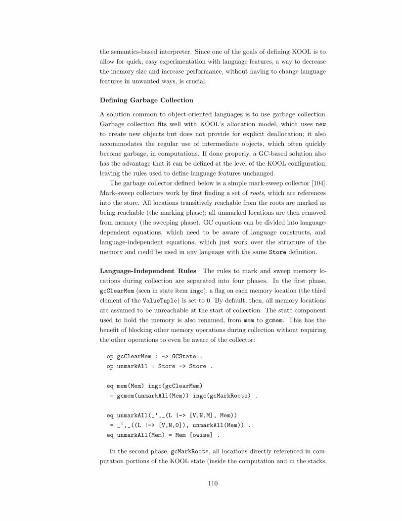
the semantics-based interpreter. Since one of the goals of defining KOOL is to
allow for quick, easy experimentation with language features, a way to decrease
the memory size and increase performance, without having to change language
features in unwanted ways, is crucial.
Defining Garbage Collection
A solution common to object-oriented languages is to use garbage collection.
Garbage collection fits well with KOOL’s allocation model, which uses new
to create new objects but does not provide for explicit deallocation; it also
accommodates the regular use of intermediate objects, which often quickly
become garbage, in computations. If done properly, a GC-based solution also
has the advantage that it can be defined at the level of the KOOL configuration,
leaving the rules used to define language features unchanged.
The garbage collector defined below is a simple mark-sweep collector [104].
Mark-sweep collectors work by first finding a set of roots, which are references
into the store. All locations transitively reachable from the roots are marked as
being reachable (the marking phase); all unmarked locations are then removed
from memory (the sweeping phase). GC equations can be divided into language-
dependent equations, which need to be aware of language constructs, and
language-independent equations, which just work over the structure of the
memory and could be used in any language with the same Store definition.
Language-Independent Rules The rules to mark and sweep memory lo-
cations during collection are separated into four phases. In the first phase,
gcClearMem (seen in state item ingc), a flag on each memory location (the third
element of the ValueTuple) is set to 0. By default, then, all memory locations
are assumed to be unreachable at the start of collection. The state component
used to hold the memory is also renamed, from mem to gcmem. This has the
benefit of blocking other memory operations during collection without requiring
the other operations to even be aware of the collector:
op gcClearMem : -> GCState .
op unmarkAll : Store -> Store .
eq mem(Mem) ingc(gcClearMem)
= gcmem(unmarkAll(Mem)) ingc(gcMarkRoots) .
eq unmarkAll(_‘,_(L |-> [V,N,M], Mem))
= _‘,_((L |-> [V,N,0]), unmarkAll(Mem)) .
eq unmarkAll(Mem) = Mem [owise] .
In the second phase, gcMarkRoots, all locations directly referenced in com-
putation portions of the KOOL state (inside the computation and in the stacks,
110

for instance, but not in the memory) are found using KStateLocs, one of the
language-dependent portions of the collector. Each of these root locations, stored
in LS, is then marked by setting the third element of the ValueTuple at that
location to 1:
op gcMarkRoots : -> GCState .
op markLocsInSet : Store LocationSet -> Store .
op mark : Store Location -> Store .
ceq threads(KS) ingc(gcMarkRoots ) gcmem(Mem )
= threads(KS) ingc(gcMarkTrans(LS)) gcmem(markLocsInSet(Mem,LS))
if LS := KStateLocs(KS) .
eq markLocsInSet(Mem, (L LS)) = markLocsInSet(mark(Mem,L), LS) .
eq markLocsInSet(Mem, emptyLS) = Mem .
eq mark(_‘,_(L |-> [V,N,M], Mem), L) = _‘,_(L |-> [V,N,1], Mem) .
Next, the third phase, gcMarkTrans, determines the locations reachable
transitively through the root locations. It works using both the iterate and
unmarkedOnly operations; the first determines the set of locations reachable in
one step from a given set of locations (if an object at location L holds references
to objects at locations L1 and L2, L1 and L2 would be reachable in one step,
but not any locations referenced by the objects at L1 or L2), while the second
filters this to only include locations that have not already been marked. At each
iteration the locations found are marked and the process continues from just
these newly-marked locations, ensuring that the traversal eventually terminates
when no new, unmarked locations are found:
op gcMarkTrans : LocationSet -> GCState .
op iterate : LocationSet Store -> LocationSet .
op unmarkedOnly : LocationSet Store -> LocationSet .
ceq threads(KS) ingc(gcMarkTrans(LS) ) gcmem(Mem )
= threads(KS) ingc(gcMarkTrans(LS’)) gcmem(Mem’)
if LS’ := iterate(LS,Mem) /\ LS’ =/= emptyLS /\
Mem’ := markLocsInSet(Mem,LS’) .
eq threads(KS) ingc(gcMarkTrans(LS)) gcmem(Mem)
= threads(KS) ingc(gcSweep ) gcmem(Mem) [owise] .
eq iterate(L LS, Mem)
= unmarkedOnly(ListToSet(valLocs(getValue(Mem,L))),Mem)
iterate(LS, Mem) .
eq iterate(emptyLS,Mem) = emptyLS .
Finally, the fourth phase, gcSweep, uses the removeUnmarked operation to
discard all memory locations not marked during the sweep performed in steps
111

two and three. It also moves the store back into mem, so other parts of the
semantics can again see the store:
op gcSweep : -> GCState .
eq ingc(gcSweep) gcmem(Mem )
= ingc(noGC(0)) mem(removeUnmarked(Mem)) .
Language-Dependent Equations Language-dependent equations are used
to gather the set of roots from the computation and any other parts of the
state (such as stacks) that may contain them. Traversal of the state is initiated
using KStateLocs, which returns a set of all locations found in a given state.
KStateLocs is defined inductively over the various state components, with other
operations specifically designed to deal with computations, computation items,
stacks, and other state components. Examples of the equations used to find the
locations inside the method stack and the computation are shown below:
op KStateLocs : KState -> LocationSet .
eq KStateLocs(mstack(MSTL) CS) = MStackLocs(MSTL) KStateLocs(CS) .
op MStackLocs : MStackTupleList -> LocationSet .
eq MStackLocs ([K,CS,Env,oref(L),Xc], MSTL)
= KLocs(K) KStateLocs(CS) ListToSet(envLocs(Env))
ListToSet(valLocs(oref(L))) MStackLocs(MSTL) .
eq MStackLocs(empty) = emptyLS .
op KLocs : Computation -> LocationSet .
eq KStateLocs(k(K) CS) = KLocs(K) KStateLocs(CS) .
eq KLocs(llookup(L) -> K) = L KLocs(K) .
KLocs deserves special comment, since it is the main operation that needs
to be modified to account for new language features. KLocs is defined for each
computation item in the language that may hold locations. This means that,
when new computation items which can contain locations are added, the collector
must be updated properly. A method of automatically transforming a theory
into one with garbage collection would eliminate this potential source of errors,
but has not yet been investigated.
Along with the equations used to find the roots, additional equations are used
to find any locations referenced by a value (for instance, the locations referenced
in the fields of an object). These equations are then used when finding the
set of locations reachable transitively from the root locations. In this case, it
was possible to reuse equations developed in earlier work [92] that were used to
find all locations reachable from a starting location so they could be marked as
shared.
Triggering Garbage Collection Garbage collection is triggered using the
triggerGC computation item:
112

op triggerGC : Nat -> ComputationItem .
This allows the language designer to decide how aggressive the collection
policy should be. Currently, triggerGC has been added to the three equations
in the memory operations that are used to allocate storage; no equations used
to define KOOL language features have been modified. The Nat included in
triggerGC contains the number of allocated locations. This is then used by the
collector to decide when to begin collecting:
ceq threads(t(control(k(triggerGC(N) -> K) CS) TS) KS) ingc(GC)
= threads(t(control(k(K) CS) TS) KS) ingc(GC)
if runningGC(GC) .
ceq threads(t(control(k(triggerGC(N) -> K) CS) TS) KS)
ingc(noGC(N’)) gccount(GN)
= threads(t(control(k(K) CS) TS) KS)
ingc(gcClearMem) gccount(s(GN))
if (N + N’) >= 1000 .
ceq threads(t(control(k(triggerGC(N) -> K) CS) TS) KS)
ingc(noGC(N’))
= threads(t(control(k(K) CS) TS) KS) ingc(noGC(N + N’))
if (N + N’) < 1000 .
The first equation just discards the trigger if the collector is already active.
The second initiates collection when 1000 or more allocations have occurred 4 –
N being the number of new allocations, N’ being the number already reported
with prior triggerGCs. The last equation increments the number of reported
allocations stored in noGC by the number of new allocations when the sum is
less than 1000.
Evaluation To evaluate the effectiveness of the garbage collector, five test
cases were executed in KOOL, both with the collector enabled and disabled.
Along with three numerical test cases, two test cases were added that were
designed to generate a large amount of garbage. The test cases were:
• factorial, recursively calculating the factorial for 20, 40, ..., 180, 200;
• ifactorial, an iterative version of factorial;
• fibonacci, a recursive algorithm computing the fibonacci numbers from 1
to 15;
41000 was chosen after some experimentation, but further experimentation could show thata different number would be better. It may also be the case that there is no ideal number –hence the prevalence of collectors with generational policies, with each generation collected atdifferent intervals.
113

GC Disabled GC EnabledTest Case Time Final Store Size Time Final Store Size Collectionsfactorial 103.060 22193 119.987 300 22ifactorial 97.100 21103 116.811 106 21fibonacci 401.334 76915 399.785 935 76addnums NA NA 516.023 946 93garbage 259.500 32013 147.211 20 32
Single 3.40 GHz Pentium 4, 2 GB RAM, OpenSuSE 10.2, kernel 2.6.18.8-0.7-default, Maude 2.3.
Times averaged over three runs of each test. All times are in seconds.
Figure 6.5: KOOL: GC Performance
• addnums, which sums the numbers 1...100, 1...200, ..., 1...1000;
• garbage, which defines a class that holds an integer and then creates a
temporary object of this class (which quickly becomes garbage) for the
numbers 1...2000.
In all cases, the total execution time was recorded. Also recorded were the
final size of the store and (in the cases where garbage collection was enabled)
the number of collections that occurred. The performance results are shown in
Figure 6.5.
At this point, results are mixed. The factorial and ifactorial tests do
not appear to benefit from garbage collection – in both cases the collector slows
performance down, even though it obviously shrinks the size of the store. The
result for fibonacci shows little difference in execution time, although again
the store is much smaller. In these three test cases, the cost of collecting either
is higher than the benefit (factorial, ifactorial) or roughly equal to the
benefit (fibonacci). However, in the final two test cases, addnums and garbage,
garbage collection obviously helps. Without GC, addnums crashes; garbage
completes in both, but is much faster with collection enabled.
One goal in developing the collector is to be able to reuse it in other languages.
Based on the current design in KOOL, this should be straight-forward. The only
part of the collector that is language-specific is the operations and equations
used to determine the set of root locations. The other parts of the collector
definition are language-independent, and can be reused directly in any language
that uses a similar (computation-based) definitional style.
6.2 Analysis Performance
The ability to model check and search programs using language definitions in
rewriting logic is very closely tied to the performance of the definition. There
are two general classes of performance improvement: improvements that impact
execution speed, and improvements that impact analysis speed, which may even
slightly reduce typical execution speed. Two examples of improvements are
presented here, both of which have appeared in various forms in programming
114

languages but not, to our knowledge, in other rewriting logic language specifica-
tions. First, auto-boxing is introduced to the language. This allows operations
on scalar types, which are represented in KOOL as objects, to be performed
directly on the underlying values for many operations (standard arithmetic oper-
ations, for instance), while still allowing method calls to be used on an object
representation of the scalar where needed. Although mainly useful in dynamic
languages like KOOL, this technique can also be used to perform automatic
coercions between scalar and object types in statically-typed languages. Second,
memory is segregated into two pools, a shared and an unshared pool. Rules are
used when accessing or modifying memory in the shared pool, since these changes
could lead to data races, while equations are used for equivalent operations on
the unshared pool. This follows the intuition that changes to unshared memory
locations in a thread cannot cause races. This change may or may not improve
execution performance, but has a dramatic impact on analysis performance.
6.2.1 Auto-boxing
In KOOL, all values, including those typically represented as scalars in languages
like Java, are objects. This means that a number like 5 is represented as an
object, and an expression like 5 + 7 is represented as a method call. Primitive
operations are defined which extract the primitive values ”hidden” in the objects
(i.e. the actual number 5, versus the object that represents it), perform the
operation on these primitive values, and create a new object representing the
result. This provides a ”pure” object-oriented model, but requires additional
overhead, including additional accesses to memory to retrieve the primitive values
and create the new object for the result. Since memory accesses are modeled
as rules in the definition, this also increases model checking and search time by
increasing the number of states that need to be checked.
To improve performance, auto-boxing can be added to KOOL. This allows
values such as 5 to be represented as scalars – i.e. directly as the primitive
values. A number of operations can then be performed directly on the primitive
representation, without having to go through the additional steps described
above. For numbers, this includes arithmetic and logical operations, which
are some of the most common operations applied to these values. Operations
which cannot be performed directly can still be treated as message sends; the
scalar value is automatically converted to an object representing the same value,
which can then act as a message target to handle the method. Since boxing can
occur automatically, by default values, including those generated as the result of
primitive operations, are left un-boxed, in scalar form. This all happens behind
the scenes, allowing KOOL programs to remain unchanged.
An example of the rule changes to enable auto-boxing is found in Figure 6.6.
The first equation is without auto-boxing. Here, when a floating point number F
is encountered, a new floating point object of class Float is created to represent
115

eq k(exp(f(F)) -> K) = k(newPrimFloat(primFloat(F)) -> K) .----------------------------------------------------------------------------------
eq k(exp(f(F)) -> K) = k(val(fv(F)) -> K) .eq k(val(fv(F),fv(F’)) -> toInvoke(n(’+)) -> K) = k(val(fv(F + F’)) -> K) .eq k(val(fv(F),Vl) -> toInvoke(Xm) -> K) =
k(newPrimFloat(primFloat(F)) -> boxWList(Vl) -> toInvoke(Xm) -> K) [owise] .
Figure 6.6: Example Definition Changes, Auto-boxing
F using newPrimFloat. Any operations on this object, such as adding two floats,
will involve a message send. The next three rules are with auto-boxing enabled.
In the second equation, instead of creating a new object for F, we return a scalar
value. The third equation shows an example of an intercepted method call.
When a method is called, the target and all arguments are evaluated, with the
method name held in the toInvoke computation item. Here, + has been invoked
with a target and argument that both evaluate to scalar float values, so we will
use the built-in float + operation instead of requiring a method call. In the fourth
equation, the boxing step is shown – here, a method outside of those handled
directly on scalars has been called with the floating-point scalar value as the
target, in which case a new object will be created just like in the first equation
([owise] will ensure that we will try this as a last resort). Once created, the
new object, and the values being sent as arguments (held in boxWList), will be
used to perform a standard method call.
Auto-boxing has a significant impact on performance. Figure 6.8 shows the
updated figures for verification times with this change in place. Not only is
this faster than the solution without auto-boxing in all cases, but it is now also
possible to verify deadlock freedom for up to 5 philosophers, which was not
possible with the prior definition.
6.2.2 Memory Pools
Memory in the KOOL definition is represented using a single global store for
an entire program. This is fairly efficient for normal execution, but for model
checking and search this can be more expensive than needed. This is because all
interactions with the store must use rules, since multiple threads could compete
to access the same memory location at the same time. However, many memory
accesses don’t compete – for instance, when a new thread is started by spawning
a method call, the method’s instance variables are only seen by this new thread,
not by the thread that spawned it. What is needed, then, is a modification to the
definition that will allow rules to be used where they are needed – for memory
accesses that could compete – while allowing equations to be used for the rest.
To do this, memory in KOOL can be split into two pools: a shared memory
pool, containing all memory accessible by more than one thread at some point
during execution, and a non-shared memory pool, containing memory that is
known to be accessed by at most one thread. To add this to the definition,
an additional global state component is added to represent the shared memory
116

pool, and the appropriate rules are modified to perform memory operations
against the proper memory pool5. Correctly moving memory locations between
the pools does require care, however, since accidentally leaving memory in the
non-shared pool could cause errors during verification.
The strategy we take to move locations to the shared pool is a conservative
one: any memory location that could be accessed by more than one thread,
regardless of whether this actually happens during execution, will be moved into
the shared pool. There are two scenarios to consider. In the first, the spawn
statement executes a message send. In this scenario, locations accessible through
the message target (an object), as well as locations accessible through the actual
parameters of the call, are all moved into the shared pool. Note that accessible
here is transitive – an object passed as a parameter may contain references to
other objects, all of which could be reached through the containing object. In
many cases this will be more conservative than necessary; however, there are
many situations, such as multiple spawns of message sends on the same object,
and spawns of message sends on self, where this will be needed. The second
scenario is where the spawn statement is used to spawn a new thread containing
an arbitrary expression. Here, all locations accessible in the current environment
need to be moved to the shared pool, including those for instance variables
and those accessible through self. This covers all cases, including those with
message sends embedded in larger expressions (since the target is in scope, either
directly or through another object reference, it will be moved to the shared
pool).
This strategy leads to a specific style of programming that should improve
verification performance: message sends, not arbitrary expressions, should be
spawned, and needed information should be passed in the spawn statement to
the target, instead of set through setters or in the constructor. This is because
the object-level member variables will be shared, while instance variables and
formal parameters will not. This brings up a subtle but important distinction –
the objects referenced by the formal parameters will be shared, but not the pa-
rameters themselves, which are local to the method, meaning that no verification
performance penalty is paid until the code needs to ”look inside” the referenced
objects. Looking inside does not include retrieving a referenced object for use in
a lock acquisition statement (however, acquisition itself is a rule).
Figure 6.7 shows one of the two rules changed to support the memory pools
(the other, for assignment, is similar), as well as part of the location reassignment
logic. The first rule, which is the original lookup rule, retrieves a value V from
a location L in memory Mem. The location must exist, which accounts for the
condition – if L does not exist, looking up the current value with Mem[L] will
return undefined. CS and TS match the rest of the control and thread states,
5Note that, although this work follows the work on execution performance in this Chapter,it actually was performed at an earlier point in time, and thus uses an older model, withseparate pools, instead of a model with a shared “bit” set on the memory location, as isdiscussed in the work on garbage collection in Section 6.1
117

crl t(control(k(llookup(L) -> K) CS) TS) mem(Mem) =>t(control(k(val(V) -> K) CS) TS) mem(Mem) if V := Mem[L] /\ V =/= undefined .
--------------------------------------------------------------------------------------------ceq t(control(k(llookup(L) -> K) CS) TS) mem(Mem) =
t(control(k(val(V) -> K) CS) TS) mem(Mem) if V := Mem[L] /\ V =/= undefined .
crl t(control(k(llookup(L) -> K) CS) TS) smem(Mem) =>t(control(k(val(V) -> K) CS) TS) smem(Mem) if V := Mem[L] /\ V =/= undefined .
ceq t(control(k(reassign(L,Ll) -> K) CS) TS) mem(Mem) smem(SMem) =t(control(k(reassign(Ll,Ll’) -> K) CS) TS) mem(unset(Mem,L)) smem(SMem[L <- V])
if V := Mem[L] /\ V =/= undefined /\ Ll’ := valLocs(V) .
ceq t(control(k(reassign(L,Ll) -> K) CS) TS) mem(Mem) smem(SMem) =t(control(k(reassign(Ll) -> K) CS) TS) mem(Mem) smem(SMem)
if V := SMem[L] /\ V =/= undefined .
eq k(reassign(empty) -> K) = k(K) .
Figure 6.7: Example Definition Changes, Memory Pools
respectively. The second and third equation and rule replace this first to support
the shared and unshared memory pools. The second is now an equation, since
the memory under consideration is not shared. The third is a rule, since the
memory is shared. This shared pool is represented with a new part of the
state, smem. The last three equations represent the reassignment of memory
locations from the unshared to the shared pool, triggered on thread creation and
assignment to shared memory locations. In the first, the location L and its value
are in the unshared pool, and are moved to the shared pool. If the value is an
object, all locations it holds references to are also added to the list of locations
that must be processed. The second represents the case where the location is
already in the shared pool. In this case, nothing is done with the location. The
third equation applies only when all locations have been processed, indicating
we should continue with the computation (with K).
This strategy could be improved with additional bookkeeping. For instance,
no information on which threads share which locations is currently tracked. Track-
ing this information could potentially allow a finer-grained sharing mechanism,
and could also allow memory to be un-shared when threads terminate. However,
even with the current strategy, we still see some significant improvements in
verification performance. These can be seen in Figure 6.9. Note that, in every
Ph No Optimizations Auto-boxingStates Counter DeadFree States Counter DeadFree
2 61 0.645 NA 35 0.64 0.7983 1747 0.723 NA 244 0.694 3.6104 47737 1.132 NA 1857 1.074 40.2795 NA 6.036 NA 14378 4.975 501.7496 NA 68.332 NA 111679 49.076 NA7 NA 895.366 NA 867888 555.791 NA8 NA NA NA NA NA NA
Single 3.40 GHz Pentium 4, 2 GB RAM, OpenSuSE 10.1, kernel 2.6.16.27-0.6-smp, Maude 2.2.
Times in seconds, Ph is philosopher count, Counter is time to generate counter-example, DeadFree
is time to verify the program is deadlock free, state count based on Maude search results, NA
means the process either crashed or was abandoned after consuming most system memory.
Figure 6.8: Dining Philosophers Verification Times
118
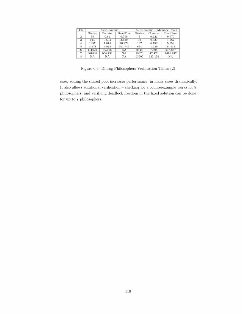
Ph Auto-boxing Auto-boxing + Memory PoolsStates Counter DeadFree States Counter DeadFree
2 35 0.64 0.798 7 0.621 0.6703 244 0.694 3.610 30 0.637 1.2874 1857 1.074 40.279 137 0.782 5.6595 14378 4.975 501.749 634 1.629 34.4156 111679 49.076 NA 2943 7.395 218.8377 867888 555.791 NA 13670 47.428 1478.7478 NA NA NA 63505 325.151 NA
Figure 6.9: Dining Philosophers Verification Times (2)
case, adding the shared pool increases performance, in many cases dramatically.
It also allows additional verification – checking for a counterexample works for 8
philosophers, and verifying deadlock freedom in the fixed solution can be done
for up to 7 philosophers.
119

Chapter 7
Policy Frameworks
Programs compute by manipulating explicit data, like integers, objects, functions,
or strings, a process captured by dynamic semantics techniques like those shown
in Chapters 3. and 4. However, program data may also have implicit properties
which cannot be represented in the underlying programming language. For
example, most languages have no way to indicate if a variable has been initialized,
or if a pointer is never null. Some languages leave types implicit, providing no
syntax to indicate types of variables or parameters.
Domain-specific examples are also common. A compelling example, commonly
used in scientific computing applications, is units of measurement, where program
values and variables are assumed to have specific units at specific points in
the program or along specific execution paths. An example from security is
information flow, where program data may have implicit security levels.
These implicit properties of program data give rise to implicit policies, or
rules about how this information can be manipulated. For instance, one may
require that variables be initialized on all paths before being read, or that only
non-null pointers can be assigned to other non-null pointers. Languages with
no explicit types generally still place type restrictions on operations such as
arithmetic, where only values representing numbers can be used. Programs that
use units of measurement must adhere to a number of rules, such as requiring
two operands in an addition or comparison operation to have the same unit, or
treating the result of a multiplication operation as having a unit equal to the
product of the units of the operands (e.g., given meter and second, the resulting
unit would be meter second). Applications concerned with information flow
need to ensure that computations do not violate security requirements.
Because these properties are hard to check by hand, a number of techniques
have been developed to make such implicit properties explicit and thus checkable
using program analysis techniques. For instance, attached types [131] have
been introduced in Eiffel to indicate when references can be null, while various
static analysis and type inference techniques have been applied to dynamically
typed languages such as Self [30, 6] to discover type information needed for
optimization.
Here, we focus on another common technique, the use of program annota-
tions, either given by “decorating” program constructs (types, variables, function
120

names, etc.) with type-like information (type annotations); or by including addi-
tional information in special language constructs (function preconditions, assert
statements, etc.) or special comments in the source code (code annotations).
Many systems that use annotations are designed with specific analysis domains in
mind; those that are more general often support either type or code annotations,
but not both, or provide limited capabilities to adapt to new domains. This chap-
ter presents a semantics-driven solution designed to overcome these limitations,
policy frameworks. A policy framework is built around a language front-end and
a core abstract rewriting logic or K semantics. The language semantics can be
purpose built for analysis, but is often built by modifying an existing static or
dynamic semantics of the language, abstracting concepts like value and modifying
semantic rules so they work appropriately for static analysis (for instance, if
the existing semantics defines standard execution behavior, the semantics used
for analysis would be modified to take both branches of a conditional, tracking
information along each).
Both the language front-end and the created core semantics are policy-generic,
treating type and code annotations as black boxes. Individual analysis domains,
such as units of measurement, then provide type and code annotations for the
domain, as well as giving an algebraic definition of the domain data. These
domains are both policy and, quite often, language generic, allowing them to
be reused across different policy frameworks. Finally, individual policies are
created as extensions to the policy framework, reusing inherited functionality,
importing specific analysis domains, extending the provided annotation systems,
and providing policy-specific semantics for language and annotation features.
Section 7.1 introduces analysis domains, providing examples both of domains
specific to a given programming language (like type systems) and more general
domains usable across multiple languages (like units of measurement). Section
7.2 then describes a policy frameworks for SILF, an imperative language also
Language
Semantics
Language Policy
Framework Core
Semantics
Domain1 Domain2 ... Domainn
Policy1 Policy2 ... Policyn
Figure 7.1: Multiple Polices in One Framework
121

Language1
Semantics
Language1 Policy
Framework Core
Semantics
Domain1
Policy1,1
Language2
Semantics
Language2 Policy
Framework Core
Semantics
Policy2,1
Figure 7.2: Domain Reuse Across Frameworks
used in Chapter 6. In Section 7.2, two policies for SILF are presented, one
for types (since SILF has no explicit types) and one for units of measurement.
This illustrates reuse within a single policy framework, with multiple policies
reusing the core framework functionality and inheriting multiple domains of
analysis, a concept illustrated graphically in Figure 7.1 (as mentioned earlier, the
policy framework core semantics may be based on an actual static or dynamic
semantics for the language, but this is optional, and there is currently no way
to automatically generate the policy semantics from an existing semantics).
This chapter presents only some of the highlights of the policy; the complete
specification for the SILF Policy Framework is provided online [88].
Looking forward, Chapter 8 will describe the C Policy Framework, or CPF,
illustrating that the policy frameworks concept can be applied to real, widely-
used languages. CPF will also support a policy for units of measurement using
the same analysis domain used for SILF. This illustrates the reuse of analysis
domains across policy frameworks, a concept illustrated graphically in Figure
7.2 (the same note applies here as applied in Figure 7.1).
7.1 Abstract Analysis Domains
Each analysis is based around an abstract analysis domain that indicates the
values manipulated by the analysis. One domain can be used across multiple
analysis policies and also across multiple policy frameworks. This section presents
two analysis domains. The first, for types, is specific to the SILF language,
providing a standard statically-checkable type system. The second, for units,
is reusable across languages, providing a domain whose values are units of
measurement. This domain is reused in Chapter 8 as part of the C Policy
Framework UNITS policy.
122

fmod TYPES is
including TYPE-ANNOTATION-HELPERS *
( sort PolicyExp to TypeExp, sort PolicyVal to Type ) .
including SILF-HELPING-OPS *
( sort PolicyExp to TypeExp, sort PolicyVal to Type ) .
sort BaseType .
subsort BaseType < Type .
ops $int $bool : -> BaseType .
op $notype : -> Type .
op $array : BaseType -> Type .
endfm
Figure 7.3: Types Domain in Maude, for SILF
7.1.1 Types
The core policy support, shared across all languages with a policy framework,
includes two sorts: PolicyVal and PolicyExp. These sorts represent generic
policy values – the abstract values manipulated by a policy – and policy expres-
sions, which are the logical formulae given in code annotations. Each policy
is expected to define the actual values and expressions usable in the policy by
adding operators which target these sorts.
Figure 7.3 shows the domain of types used in the SILF type checking policy, de-
fined in Maude. Two modules are imported: TYPE-ANNOTATION-HELPERS, which
provides operators for working with type annotations; and SILF-HELPING-OPS,
which provides operators for working with the SILF configuration. Both modules
map PolicyVal and PolicyExp to sort names more appropriate for the policy:
PolicyExp to TypeExp, PolicyVal to Type.
Using these imported sorts, several additional operators are defined. SILF
provides both integers and booleans. A new sort, BaseType, is created with
two constructors, $int and $bool, representing these basic types. BaseType
is a subsort of Type, allowing terms of sort BaseType to also be used as types
(i.e., as policy values). The type $notype is given to represent situations where
no type is given in a SILF program (for instance, on an unannotated variable
declaration) – this is needed because types are not required in the language
syntax. Finally, since SILF support arrays, a type for arrays, $array, is also
defined. $array takes a base type as a parameter, meaning it is possible to form
arrays of integers or booleans, but not of $notype or other array types.
7.1.2 Units of Measurement
Figure 7.4 shows the basic axiomatization of the units domain, used in the
units of measurement checking policies for both SILF and C. Like with the
types domain, shown above, the units domain renames sorts PolicyExp and
PolicyVal, given them names more appropriate to the domain: UnitExp and
Unit. A new sort, BaseUnit, is also introduced and made a subsort of Unit.
123

fmod UNITS is
protecting RAT .
including TYPE-ANNOTATION *
( sort PolicyExp to UnitExp, sort PolicyVal to Unit ) .
sorts BaseUnit .
subsort BaseUnit < Unit .
ops $noUnit $fail $cons : -> BaseUnit .
op _^_ : BaseUnit Rat -> BaseUnit [prec 10] .
op __ : BaseUnit BaseUnit -> BaseUnit [assoc comm prec 15] .
op _^_ : Unit Rat -> Unit [ditto] .
op __ : Unit Unit -> Unit [ditto] .
op NUnit : Nat -> BaseUnit .
vars U U’ : Unit . vars N M : Rat .
eq U $noUnit = U .
eq U $fail = $fail .
eq U $cons = U .
eq $fail ^ N = $fail .
eq $noUnit ^ N = $noUnit .
eq $cons ^ N = $cons .
eq U ^ 0 = $noUnit .
eq U ^ 1 = U .
eq U U = U ^ 2 .
eq U (U ^ N) = U ^ (N + 1) .
eq (U ^ N) (U ^ M) = U ^ (N + M) .
eq (U U’) ^ N = (U ^ N) (U’ ^ N) .
eq (U ^ N) ^ M = U ^ (N * M) .
endfm
Figure 7.4: Units Domain
The rest of the module shown in Figure 7.4 defines a number of operators, used
to construct units, and equations, used to determine when two units are equal.
Several “pseudo-units” are defined as base units: $noUnit, $fail, and $cons.
$noUnit represents values with no assigned unit (for instance, loop counters
iterating through an array); $fail represents a unit error, and is used as the
result of an invalid computation; and $cons represents the unit of a constant,
allowing constants to be used in standard calculations without explicitly declaring
a unit. The next four operators define ways to build units: a unit (or base unit)
can be raised to a rational power, and the product of two units, represented
by placing the units together, is also a unit. Finally, the NUnit operator allows
for the creation of unique “fresh” units, providing a way to generate units in
situations where the actual unit is unknown, such as with unannotated function
parameters. The use of globally unique units cuts down on spurious warnings,
allowing operations like multiplication, which do not require the units to be the
same, to be performed safely even on unknown units.
The equations then are used to normalize units and determine when two
units are equal. For instance, eq (U ^ N) (U ^ M) = U ^ (N + M) states
that, given two units U ^ N and U ^ M, the product of these units is the same
as U ^ (N + M).
Figure 7.5 then shows a number of actual units, built on the unit axiomatiza-
124

fmod BASIC-UNITS is
protecting UNITS .
*** Length.
ops $meter $m : -> BaseUnit .
*** Mass.
ops $kilogram $kg : -> BaseUnit .
*** Time.
ops $second $s : -> BaseUnit .
*** Electric current.
ops $ampere $A : -> BaseUnit .
*** Thermodynamic temperature.
ops $kelvin $K : -> BaseUnit .
*** Amount of substance.
ops $mole $mol : -> BaseUnit .
*** Luminous intensity.
ops $candela $cd : -> BaseUnit .
endfm
fmod DERIVED-UNITS is
including BASIC-UNITS .
*** Frequency
ops $hertz $Hz : -> BaseUnit .
eq $hertz = $s ^ -1 .
*** Force
ops $newton $N : -> BaseUnit .
eq $newton = $m $kg $s ^ -2 .
*** Pressure, stress
ops $pascal $Pa : -> BaseUnit .
eq $pascal = $m ^ -1 $kg $s ^ -2 .
*** Magnetic flux density
ops $tesla $T : -> BaseUnit .
eq $tesla = $kg $s ^ -2 $A ^ -1 .
*** Catalytic activity
ops $katal $kat : -> BaseUnit .
eq $katal = $s ^ -1 $mol .
endfm
Figure 7.5: Units Domain, Part 2
tion given in Figure 7.4. Module BASIC-UNITS shows short and long forms of the
basic units for each of the seven base dimensions that make up the International
System of Units (SI) [5]. Equations, not shown, equate each form, allowing either
to be used in annotations. Module DERIVED-UNITS then shows several examples
of units derived from these base units, along with equations which equate each
derived unit with the actual base units the derived unit represents.
7.2 The SILF Policy Framework
The SILF language was introduced in Chapter 6, with the concrete syntax
shown in Figure 6.1. SILF provides a conceptually simple language in which to
introduce the concept of policy framework, with enough complexities (global
variables, function calls, arrays) to highlight challenges but without some of the
difficulties of a language like C (function pointers, pointer arithmetic, aliasing,
unions, etc).
7.2.1 Adding a Policy Framework to SILF
To create policies in SILF, the first step is to add the shared parts of a policy
framework: an annotation-generic front-end and a core semantics.
SILF Policy Framework Front-end
The front-end for the SILF Policy Framework (SILF-PF) is an extended version
of the existing SILF parser. Since SILF is a language that we have designed,
125

Declarations D ::= ... | var TI | var TI[N ]
Statements S ::= ... | for I := E to E IVl do S od | while E IVl do S od |
assert(I): ann; | assume(I): ann;
Function Declarations FD ::= function TI(TIl) PPl begin S end
Typed Identifiers TI ::= I | tann I | tvar I
Typed Identifier Lists TIl ::= TI (, T I)∗
| void
Invariants IV ::= inv(I): ann; | invariant(I): ann;
Invariant Lists IVl ::= IV ∗
PrePosts PP ::= pre(I): ann; | precond(I): ann; | post(I): ann; |
postcond(I): ann; | mod(I): ann; | modifies(I): ann;
PrePost Lists PPl ::= PP∗
Figure 7.6: Extended Policy Syntax for SILF
the language is extended directly to support policy frameworks, versus adding
policy annotations through comments given in program source. The original
syntax for SILF was given in Figure 6.1 in Chapter 6; Figure 7.6 shows just the
modifications to this syntax made to enable policy frameworks.
Type annotations are identifiers with a leading $, like $int or $meter, and
are represented in the BNF with tann. tvar represents a type variable, given
with similar syntax: $$, instead of just $, like $$X. These are added in the syntax
with Typed Identifiers, which also includes unannotated identifiers, and are then
allowed in the productions for both variable and function declarations.
Code annotations are added by extending the language with new constructs
for invariants on loops (for both while and for loops), assume and assert
statements, and, in function declarations, function contracts with preconditions,
postconditions, and modifies (which identifies the globals changed by a function).
The syntax for each of these is given in the BNF: PrePosts for function contracts
(with short and long forms for preconditions, postconditions, and modifies),
Invariants for loop invariants, and extensions to the statement syntax for assumes
and asserts. The code annotation. an arbitrary string, is itself represented with
ann, and is actually parsed by the policy.
Each code annotation includes a policy tag, identifying the policy associated
with the annotation language used in the annotation. This policy tag is just an
identifier, given using I, and is given before the annotation, like in pre(I).
SILF Core Policy Semantics
The core semantics includes the original SILF abstract syntax, extended with the
new type and code annotation constructs mentioned above, and the configuration
(i.e., K cells). The original dynamic semantics can be viewed as a special policy
which ignores the additional constructs, with evaluation over a concrete, versus
abstract, domain. Extensions for policies include modules providing: basic logical
connectives; pretty printing capabilities for generating error messages; support
for type annotation variables with limited forms of polymorphism; additional K
cells for analysis information; and operators for working with these extensions.
126

〈k〉 X := E(X, E) y checkAssign(X, E)
...〈/k〉 (7.3)
〈k〉 X[E] := E′
(X, E, E′) y checkArrayAssign(X, E, E′)...〈/k〉 (7.4)
〈k〉 if E then Dt St else Df Sf fiE y checkIfGuard(E) y if (E, Dt y St y Env , Df y Sf y Env)
...〈/k〉
〈env〉Env〈/env〉 (7.5)
Figure 7.7: SILF Abstract Statement Semantics
K’s modularity allows new cells to be added without requiring changes to existing
rules, making it easy to extend the state with new analysis information, such as
line numbers (cell currLn), a copy of the environment current at function entry
(cell old), and error messages generated by the analysis (cell log).
Placeholders: In addition to the extensions mentioned above, each SILF
language feature is given a default generic semantics, which can then be extended
as needed by individual policies. In some cases this semantics just provides
support for part of a computation, expecting the policy to provide the other
rules. For instance, addition expressions use the following generic rule:
E + E′ → (E,E′) y plus(E + E′) (7.1)
This rule says that, to process an expression like E + E′, first evaluate E and
E′. To remember what to do with the results, the rule uses a new operator plus,
like what was described in Chapter 2. plus takes an expression, here the original
expression (E + E′), which is kept solely in case it is needed to help generate an
error message using a syntax pretty printer. In some other cases, the generic
semantics provides specific hooks that are to be given meaning by policies. The
rule for evaluating a number expression is:
N → defaultIntVal (7.2)
Different policies can then give different definitions for defaultIntVal, such as
$int for a types policy or $cons (for constant) for a units policy. All analysis
rules for handling standard SILF expressions (arithmetic, logical, and boolean
operations) use similar techniques, deferring decisions about correctness to the
actual policy.
Statement Handling: Statements in the policy framework for SILF are given
a generic semantics, again often with hooks to policy-specific functionality.
Figure 7.7 provides several examples of semantic rules for statements. Rule
(7.3) is the generic rule for assignments. To check an assignment, the semantics
127

function TX (TXs) PPl begin Dl Sl end (7.6)
checkRetType(TX ) y checkSigTypes(TXs) y Dl y saveRetType(TX ) y Sl y dropRetType(7.7)
checkCall(TX ,TXs) y getRetTypeForCall(TX ) (7.8)
checkRetType(TX ) y checkSigTypes(TXs) y applyPM (PPl) y checkPoint y Dl y
saveRetType(TX ) y savePostConds(PPl) y Sl y dropRetType y dropPostConds(7.9)
checkAndBindCall(TX ,TXs) y checkPreConds(PPl) y applyHavoc(PPl) y
getRetValForCall(TX ,PPl) (7.10)
Figure 7.8: SILF Abstract Function Computations
first evaluates X and E. The computation item checkAssign then checks, in a
policy-specific manner, whether the value of E can be assigned to X, based on the
value of X. Rule (7.4) is similar, but also evaluates the array index expression,
and then uses computation item checkArrayAssign to ensure the assignment
meets all requirements for the policy. The final rule shown, Rule (7.5), shows the
generic semantics for a conditional. The conditional guard, E, is evaluated first;
the computation item checkIfGuard will then check the value in a policy-specific
manner. Next, computations are built into the if computation item for both
branches, ensuring that declarations and statements are both processed and that
the environment is reset to the environment active before the branch to properly
handle scoping.
Handling Functions: In the SILF dynamic semantics, a SILF program is
processed by storing a computation for each function in a function table, fenv,
and then invoking the main function’s computation (which can, in turn, invoke
other functions in the table). In the policy semantics, all functions should be
checked, which can be accomplished by invoking each in turn and evaluating
each using the policy semantics. Function calls should not actually result in a
transfer of control to another function. A second function table, ftenv, stores
information about the function which can instead be used to check each call site.
In summary, fenv and ftenv each have one entry per function; each entry in fenv
is run once for each function f , to analyze the function; this analysis will trigger
entries for each function f ′ in ftenv to be run once for each call to f ′ in f .
Figure 7.8 shows the abstract syntax for a function (in (7.6)) and the compu-
tations built for analysis that are stored as the function semantics in fenv and
ftenv. The function consists of a potentially type annotated function name (TX ),
potentially type annotated function parameters (TXs), code annotations (PPl),
and then the function declarations (Dl) and statements (Sl). The computations
128

are placed in the k cell as part of the analysis step, running the function for
analysis, and referencing the parts of the function listed above (i.e., when a
computation references TXs, this is the TXs from the function). The first two
computations, the first present in fenv as the analysis semantics for the function,
the second present in ftenv for analyzing individual call sites, are for policies
without code annotations; the second two, involving the same cells, are for
policies with code annotations.
In the first computation (7.7), checkRetType checks the return type annota-
tions in a policy specific manner (the type checking policy defined below just
verifies an annotation is given, for instance). checkSigTypes does the same with
the formal parameters, while saveRetType retrieves the return type annotations
and saves them in the state, allowing them to be checked at any return statements
inside the function body. Dl, a declaration list, is evaluated to process any
local declarations in the function, while Sl is processed to evaluate the function
body. At the end of function processing, dropRetType removes the return type
annotations from the state.
The third computation (7.9) is very similar, with checkRetType, checkSig-
Types, saveRetType, and dropRetType all playing the same roles as in the first
computation. applyPM, given a list of code annotations PPl, is used to apply
the preconditions and modifies clauses for this policy. This occurs after type
annotations are checked but before any declarations are processed in the function.
Preconditions will assume facts given in their policy expressions, while modifies
will unlock any listed global variables (which are all locked on function entry)
so they can be changed inside the function. checkPoint will then capture the
current state as the old state, so it can be referenced in other annotations. Next,
savePostConds saves any postconditions in the state, similarly to how return type
annotations are saved; this way they can be referenced during the processing
of return statements, to ensure that, at function return, they hold. Finally,
dropPostConds removes saved postcondition information when function analysis
is done.
The second (7.8) and fourth (7.10) computations are much simpler. Both
assume that a list of policy values, representing actual arguments to the function
call, is provided. checkCall will then compare each provided value with the value
of the formal parameter, looking for errors. Additional checking is also performed,
such as verifying the correct number of arguments is given. checkAndBindCall is
similar, but it will also bind policy values to the formal parameters, since they
may be accessed in annotations. checkPreConds verifies that preconditions hold
at call sites, while applyHavoc will clear any globals mentioned in a modifies
clause, since the globals are assumed to hold a random value after the function
call. Finally, getRetTypeForCall and getRetValForCall both retrieve the return
value for the call, with the latter also taking any postconditions (with assignments
to @result, representing the return value of the function) into account.
129
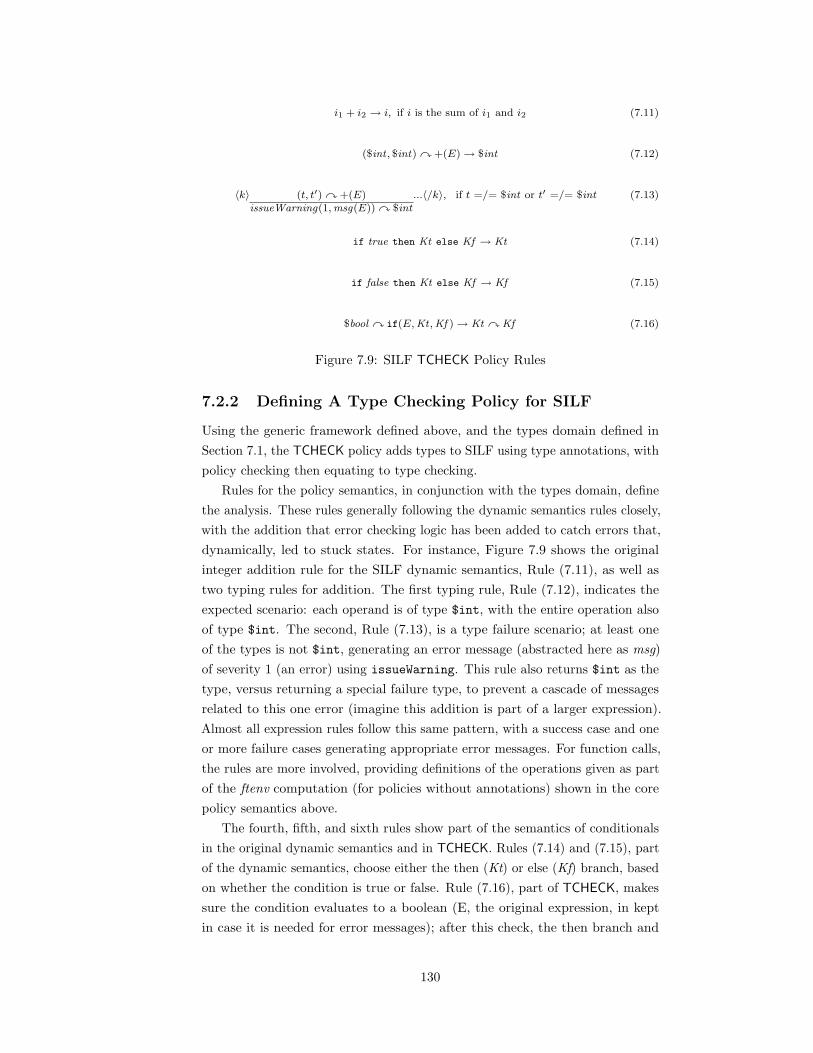
i1 + i2 → i, if i is the sum of i1 and i2 (7.11)
($int , $int) y +(E)→ $int (7.12)
〈k〉 (t, t′) y +(E)issueWarning(1,msg(E)) y $int
...〈/k〉, if t =/= $int or t′ =/= $int (7.13)
if true then Kt else Kf → Kt (7.14)
if false then Kt else Kf → Kf (7.15)
$bool y if(E,Kt ,Kf )→ Kt y Kf (7.16)
Figure 7.9: SILF TCHECK Policy Rules
7.2.2 Defining A Type Checking Policy for SILF
Using the generic framework defined above, and the types domain defined in
Section 7.1, the TCHECK policy adds types to SILF using type annotations, with
policy checking then equating to type checking.
Rules for the policy semantics, in conjunction with the types domain, define
the analysis. These rules generally following the dynamic semantics rules closely,
with the addition that error checking logic has been added to catch errors that,
dynamically, led to stuck states. For instance, Figure 7.9 shows the original
integer addition rule for the SILF dynamic semantics, Rule (7.11), as well as
two typing rules for addition. The first typing rule, Rule (7.12), indicates the
expected scenario: each operand is of type $int, with the entire operation also
of type $int. The second, Rule (7.13), is a type failure scenario; at least one
of the types is not $int, generating an error message (abstracted here as msg)
of severity 1 (an error) using issueWarning. This rule also returns $int as the
type, versus returning a special failure type, to prevent a cascade of messages
related to this one error (imagine this addition is part of a larger expression).
Almost all expression rules follow this same pattern, with a success case and one
or more failure cases generating appropriate error messages. For function calls,
the rules are more involved, providing definitions of the operations given as part
of the ftenv computation (for policies without annotations) shown in the core
policy semantics above.
The fourth, fifth, and sixth rules show part of the semantics of conditionals
in the original dynamic semantics and in TCHECK. Rules (7.14) and (7.15), part
of the dynamic semantics, choose either the then (Kt) or else (Kf) branch, based
on whether the condition is true or false. Rule (7.16), part of TCHECK, makes
sure the condition evaluates to a boolean (E, the original expression, in kept
in case it is needed for error messages); after this check, the then branch and
130

the else branch are both checked. Rules for other statements are very similar,
checking to ensure that arguments are of the correct type (for loops expect
integers as the index start and end, for instance) and then checking the body of
the statement.
Figure 7.10 shows an example run of the TCHECK policy. A program with
type errors is shown in the top portion of the figure, with the generated error
messages shown below. Policies define extensions to the default pretty printer
operations to print their own type annotations, such as $int in the second and
third error messages.
7.2.3 Defining a Units Policy for SILF
Again starting with the core semantics, the SILF-PF UNITS policy is designed
to check for unit safety in SILF programs. A program is considered unit safe
if it properly follows a number of unit rules, such as only adding values with
matching units. These rules are codified in the UNITS policy semantics. The
rules in UNITS use units as policy values, similarly to the way that TCHECK
used types. The domain of units was presented in Section 7.1.
In many cases units can be treated the same as types, with similar semantic
rules to those already shown for TCHECK. Figure 7.11 shows several UNITS
rules. The first, Rule (7.17), is for addition, where, if both units match, the
result is the same unit; Rule (7.18) is an error case for addition, where the units
don’t match and the second unit isn’t a constant (which can be converted to
any unit).
Rule (7.19) is a rule for multiplication, where the resulting unit is the product
of the operand units. The fourth rule, Rule (7.20), is a rule for less-than, similar
1 function $int f($int x)
2 begin
3 return x + 1;
4 end
5 function $int main(void)
6 begin
7 var $int x;
8 x := 3;
9 x := f(x);
10 x := f(x,x);
11 if x then write 1; else write 2; fi
12 if (x < 5) then write 1; else write false; fi
13 end
Type checking found errors:
ERROR on line 10: Type failure: too many
arguments provided in call to function f.
ERROR on line 11: Type failure: expression x
should have type $bool, but has type $int.
ERROR on line 12: Type failure: write expression
false has type $bool, expected type $int.
Figure 7.10: Type Checking using TCHECK
131

(u, u) y +(E)→ u (7.17)
〈k〉 (u, u′) y +(E)issueWarning(1,msg(E)) y $fail
...〈/k〉, if u =/= u′ and u′ =/= $cons (7.18)
(u, u′) y ∗(E)→ uu′ (7.19)
(u, u) y< (E)→ $noUnit (7.20)
V y if(E,Kt ,Kf )→ Kt y Kf (7.21)
〈k〉(u, u′) y checkAssign(X, E)·
...〈/k〉, if u == u′ or u′ == $cons (7.22)
〈k〉(u, u′) y checkAssign(X, E)issueWarning(1,msg(X, E))
...〈/k〉, if u =/= u′ and u′ =/= $cons (7.23)
Figure 7.11: SILF UNITS Policy Rules
to addition but returning $noUnit, since booleans do not have associated units
(the error rule is similar to that for addition and is not shown).
Rules (7.21), (7.22), and (7.23) are rules for statements. Rule (7.21) handles
conditionals, and is similar to Rule (7.16) in the TCHECK policy, except there
is no need to check the value computed by the guard – any errors found in the
guard expression will have already been reported, and the guard is not expected
to have a specific unit (a more stringent requirement would be to enforce that
the guard has no unit, but that is not done here). Rules (7.22) and (7.23) then
show the regular and error cases for assignment. In Rule (7.22), the assignment
is safe if the value being assigned either has the same unit or is a constant; in
Rule (7.23), this condition does not hold, so an error message is issued.
An example run of a UNITS policy analysis is shown in Figure 7.12. Function
id returns whatever it is given, making it polymorphic on the input unit. The
errors on line 10 are standard arithmetic unit errors, while the error on line 13
is triggered by a conflict in the type of y and the postcondition of id.
Note that invariants have not come up in either policy. Up until now, they
have not been needed. If the units assigned to a variable can change over time,
for instance in each iteration of a loop, an invariant becomes essential. Since
invariants are used in CPF, their discussion is deferred until Chapter 8.
132

1 function id(x)
2 post(UNITS): @unit(@result) = @unit(x);
3 begin
4 return x;
5 end
6 function main(void)
7 begin
8 var $m x;
9 var $f y;
10 x := x + y;
11 x := id(x);
12 y := id(y);
13 y := id(x);
14 end
Unit errors found:
ERROR on line 10: Assigning incompatible unit
to explicitly annotated variable: x has
unit $meter,(x + y) has unit $fail
ERROR on line 10: Unit failure, attempting to
add incompatible units: (x + y),$meter,$feet
ERROR on line 13: Assigning incompatible unit
to explicitly annotated variable: y has
unit $feet, (id(x)) has unit $meter //
Figure 7.12: Unit Checking using UNITS
133

Chapter 8
The C Policy Framework
The C Policy Framework is an application of the Policy Frameworks concept,
described in Chapter 7, to the C language. Section 8.1 describes the CPF
frontend and annotation support, including a description of the process used to
inline annotations in C code and generate function-level analysis tasks. Examples
from the C abstract syntax used by CPF are then given in Section 8.2, while
Section 8.3 describes the K cells used in the CPF analysis configuration. The
policy-generic semantics are described in Section 8.4, with a special focus on the
analysis semantics given C statements. Two policies are then presented. The
first, the UNITS policy, is the CPF-equivalent of the UNITS policy for SILF
shown in Chapter 7, and is shown in Section 8.5. Section 8.6 then shows a
simple memory policy for guarding again null dereferences of C pointers. Finally,
Section 8.7 presents a discussion of some of the challenges and limitations of the
policy frameworks approach and the C Policy Framework.
8.1 CPF Frontend and Annotation Support
CPF supports both type and code annotations. Code annotations are provided
as comments added to the original C source. CPF annotations are differenti-
ated from standard comments with an @: /*@ for traditional “C-style” com-
ments, //@ for line comments. Supported annotations include: precondition
(pre), postcondition (post), and modifies (mod) in function headers; assume,
assert, and invariant in function bodies; and tinvariant (type invariant) on
structures and unions. Annotations also include the name of the policy, allowing
different annotations to be added for different policies; annotations with policy
ALL, or no policy, apply to all policies.
As a motivating example, Figure 8.1 shows an example of a simple function
1 #include <stdlib.h>
2 int * f(int x) {
3 int *p;
4 p = (int*)malloc(sizeof(int));
5 *p = x;
6 return p;
7 }
Figure 8.1: A Potential Pointer Error
134

1 double sqrt(double x);
2
3 double lb2kg(double w) {
4 return (10 * w / 22);
5 }
6
7 double e2s(double e, double w) {
8 return sqrt(2 * e / w);
9 }
10
11 int main() {
12 double pw = 5; double e = 2560;
13 double speed = e2s(e,lb2kg(pw));
14 }
Figure 8.2: Implicit Units
that allocates a new integer pointer, assigns it the value of x, and then returns
the pointer. Although the intention is that this function should return a non-null
pointer, there is no way to indicate this. In fact the function violates this intent,
since malloc may return a null pointer (also causing a potential error on line 5).
Another example is provided in Figure 8.2. This time the example is a
fragment of a scientific application manipulating values with associated units of
measurement. Without any direct way to represent the units, even with a short
code fragment it is not clear that this code is unit safe.
Figure 8.3, an annotated version of Figure 8.1, shows an example of a CPF
type annotation. Type annotations can be added wherever types are used in the
program: on variables, function headers, structure definitions, casts, etc. Here, a
$notnull annotation is added to the function type to indicate that the function
should always return a definitely not null pointer, a fact that can be used when
analyzing clients of this function.
Examples of CPF code annotations, including pre, post, and assume, are
shown in Figure 8.4, an annotated versions of the program fragment shown in
Figure 8.2. Type annotations are also used, since they can be mixed in the same
program. The figure shows examples of annotations (such as $kg and $lb) used
to identify the units associated with various program values.
Once the source code has been annotated, it is parsed to allow annotations
(in both styles) to be read and analysis tasks, one per function, to be generated.
Parsing takes place in two phases. First, a simple transformation is applied to
move annotations from comments or types into language syntax, producing a
1 #include <stdlib.h>
2 int * $notnull f(int x) {
3 int *p;
4 p = (int*)malloc(sizeof(int));
5 *p = x;
6 return p;
7 }
Figure 8.3: Adding Pointer Annotations
135

1 //@ post(UNITS): @unit(@result) ^ 2 = @unit(x)
2 //@ modifies: @nothing
3 double sqrt(double x);
4
5 //@ pre(UNITS): @unit(w) = $lb
6 //@ modifies: @nothing
7 double $kg lb2kg(double w) {
8 return (($kg) (10 * w / 22));
9 }
10
11 //@ post(UNITS): @unit(@result) ^ 2 = @unit(e) (@unit(w) ^ -1)
12 //@ modifies: @nothing
13 double e2s(double e, double w) {
14 return sqrt(2 * e / w);
15 }
16
17 int main() {
18 double $lb pw = 5; double e = 2560;
19 /*@ assume(UNITS): @unit(e) = $kg $m ^ 2 $s ^ -2 */
20 double speed = e2s(e, lb2kg(pw));
21 }
Figure 8.4: Unit Annotations
program using a CPF-extended C syntax that directly supports annotations.
The second phase takes this modified version of the source, preprocesses it
using a standard C preprocessor, then parses the preprocessed source using a
modified version of the CIL parser for C [154], generating an internal, AST-like
representation of the code. This internal representation knows about the CPF
extensions, but does not know about the policy-specific annotation languages
used in the annotations, allowing the parser to remain policy generic.
After parsing, two custom CIL passes prepare the code for policy analy-
sis. The first simplifies function call sites and return statements by moving
all computation before the call or return. The second replaces call sites with
CPF statements to enforce the annotation semantics: assert for precondi-
tions, assume for postconditions, and havoc, which assigns a random value,
for modifies. Annotations on function headers are moved to the start of the
function body, with preconditions becoming assumes and modifies becoming
unlocks, which allows formal parameters and globals, locked against changes by
default, to be modified. Postconditions become asserts at each return state-
ment. Individual analysis tasks for each function are then generated in a format
readable by Maude.
An example analysis task, for function e2s in Figure 8.4, is shown in Figure 8.5.
It starts with 5 declarations, including for formal parameters and temporaries
added by CIL; an empty unlock (because of an empty modifies clause); a
checkpoint to save the starting state; and then the function body, including a
call to sqrt (the location of the call is marked in case it is needed by the policy).
sqrt has no precondition; it has an empty modifies, leading to an empty
havoc, and its postcondition (see Figure 8.4) generates the assume. Finally,
136

1 #CPFLine 13 decl(double, did(nf(’e)))
2 decl(double, did(nf(’w)))
3 decl(double, did(n(’tmp)))
4 decl(double, did(nt(’__cil_tmp4)))
5 decl(double, did(nt(’__cil_tmp5))) {
6 #CPFLine 14 #CPFUnlock(n(’UNITS),@nothing);
7 #CPFLine 14 #CPFCheckpoint
8 #CPFLine 14 (nt(’__cil_tmp4) =
9 ((i(2) * nf(’e)) / nf(’w))) ;
10 #CPFLine 14 #CPFCall("sqrt")
11 #CPFLine 14 #CPFHavoc(n(’UNITS),@nothing);
12 #CPFLine 14 #CPFAssume(n(’UNITS),
13 unit(n(’tmp)) ^ 2 =
14 unit(nt(’__cil_tmp4))); {
15 #CPFLine 14 (nt(’__cil_tmp5) = n(’tmp)) ; {
16 #CPFLine 14 #CPFIAssert(n(’UNITS),
17 unit(crrnt(nt(’__cil_tmp5))) ^ 2 =
18 unit(nf(’e)) unit(nf(’w)) ^ -1);
19 #CPFLine 14 return nt(’__cil_tmp5) ;}}}
Figure 8.5: Generated Code for Analysis
an assert1 is inserted before the return, verifying that the unit of the value
to be returned matches the annotation given for the postcondition. #CPFLine
directives keep track of the current line, used in error messages.
Running CPF The general process used to process analysis tasks with CPF
is shown in Figure 8.6. First, an annotated source file is processed by the
annotation processor and parser; this process generates multiple analysis tasks,
one for each function defined in the source file. These analysis tasks, along
with the policy to be checked, are then handed to Maude; the core and policy
semantics are read first, with the analysis tasks, encoded as Maude terms, then
each evaluated. When this process terminates, the results generated by policy
checking are displayed to the user. Messages logged during analysis include a
number representing the severity of the message (i.e., 1 for error, 2 for warning,
etc.), and can be filtered appropriately, allowing a policy to define a severity for
1CPFIAssert, used here, is like a normal assert, but is executed in the starting environmentcaptured when the state is checkpointed. crrnt is then used to access the current, not thestarting, environment. Another option would be to make crrnt the default and instead providean operation like old to access the initial state.
Annotated C
Source
Annotation
Processor/
Parser
Maude
Policy
Checking
ResultsAnalysis
Tasks
Core
Framework
SemanticsPolicy
Semantics
Figure 8.6: Framework Execution Model
137

1 op _+_ : Exp Exp -> Exp .
2 op if__else_ : Exp Stmt Stmt -> Stmt .
3 op return_; : Exp -> Stmt .
4 op assume_; : PolicyExp -> Stmt .
5 op @unit : Exp -> Unit .
Figure 8.7: CPF C Abstract Syntax
each issued warning.
8.2 Abstract Syntax
An extended abstract syntax of C is defined as part of the policy framework to
allow semantic rules and equations (hence referred to as just rules unless the
distinction is important) to be written over a syntax as close to native C syntax
as possible. Syntactic categories, such as expressions and statements, are defined
as sorts, with operations defined for each syntactic construct, generally using
mixfix notation, which allows a style of definition accessible to those familiar
with notations such as BNF. Syntactic constructs include abstract forms of
standard C language constructs and constructs added by CIL during analysis
task generation, including: new statements for assume and assert annotations;
representations of abstract values, such as the unit values shown in Figures 7.4
and 7.5; and syntax for expressions used inside annotations, such as the @unit
annotation shown in Figure 8.4. In addition, a number of “helper” operations
written to work with the abstract syntax have been defined, to perform tasks
such as checking whether an identifier represents a formal parameter or whether
a declaration of a variable is of a structure type.
Figure 8.7 shows several examples of the CPF C abstract syntax with the
extensions mentioned above. The first operation defines the + operator as
taking two expressions (one for each underscore) and yielding an expression; the
second and third similarly define the if (including an else clause) and return
statements. The fourth is for the assume statement, added to programs during
CIL processing to represent assume annotations. Finally, the fifth is the @unit
operation, part of the UNITS policy, used inside annotations to get or set the
unit associated with a C object (a memory region that can be read or written).
8.3 K Cells
CPF includes the definition of a generic computation used by the semantic
rules to keep track of information needed by or produced during analysis. A
number of individual K cells make up this computation, including: the abstract
computation, k; the current environment, env; the environment on function
entry, origenv, used in annotations generated for postconditions or where the
138

State
OutputSet
Env
Computation
out
k
Nat
nextloc
env
EnvSet
envs
Nat
currLn
Env
origenv
StructMap
GotoMapstructMap
gotoMap
Figure 8.8: Framework Configuration
annotation requests the old value of an expression; a set of all environments, envs,
the need for which is explained below; out, containing output messages generated
during policy checking; nextLoc, holding the next (abstract) memory location
to allocate; currLn, the current line number from the original source program;
structMap, containing definitions of all structures and unions used by the function
being analyzed; and gotoMap, used when processing goto statements to keep
track of jump destinations. Individual policies can extend this with information
needed by the policy semantics. Rules will then change the information in one or
more of these cells as analysis proceeds, such as by adding new mappings from
names to values in env or modifying the abstract computation in k. A graphical
representation of the CPF configuration is shown in Figure 8.8.
Environments CPF statements and expressions are each evaluated in the
context of an environment, the definition of which is shown in Figure 8.9. An
individual entry in the environment contains an identifier (set to a default
value for C objects that are not associated with a distinct identifier, such as
list->next->x), an abstract location, an abstract value, and EnvItem, which
is a set of additional environment information which can be extended to meet
the needs of a specific policy. The concept of Value is also policy-specific, and
can represent individual values or collections of values (lists, sets, etc.). These
individual entries are combined into a set to make up the program environment,
with operators and structural equations provided to retrieve the value at a
specific name or location.
CPF statements then each return a set of environments as a result of execution,
with each environment in the set being the result of execution along a distinct
control flow path (i.e., the branches of a conditional, the cases of a switch,
paths created using goto, etc.). Merging the different environments in the set
is then done in a policy-specific manner. For instance, some policies may want
to combine returned values, for instance by using ⊤ and ⊥ to represent over
or under-determined values; others may want to track a set of possible values,
139
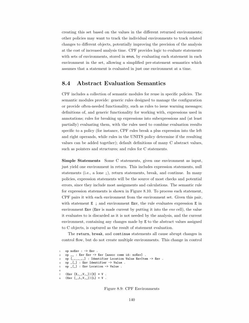
creating this set based on the values in the different returned environments;
other policies may want to track the individual environments to track related
changes to different objects, potentially improving the precision of the analysis
at the cost of increased analysis time. CPF provides logic to evaluate statements
with sets of environments, stored in envs, by evaluating each statement in each
environment in the set, allowing a simplified per-statement semantics which
assumes that a statement is evaluated in just one environment at a time.
8.4 Abstract Evaluation Semantics
CPF includes a collection of semantic modules for reuse in specific policies. The
semantic modules provide: generic rules designed to manage the configuration
or provide often-needed functionality, such as rules to issue warning messages;
definitions of, and generic functionality for working with, expressions used in
annotations; rules for breaking up expressions into subexpressions and (at least
partially) evaluating them, with the rules used to combine evaluation results
specific to a policy (for instance, CPF rules break a plus expression into the left
and right operands, while rules in the UNITS policy determine if the resulting
values can be added together); default definitions of many C abstract values,
such as pointers and structures; and rules for C statements.
Simple Statements Some C statements, given one environment as input,
just yield one environment in return. This includes expression statements, null
statements (i.e., a lone ;), return statements, break, and continue. In many
policies, expression statements will be the source of most checks and potential
errors, since they include most assignments and calculations. The semantic rule
for expression statements is shown in Figure 8.10. To process each statement,
CPF pairs it with each environment from the environment set. Given this pair,
with statement E ; and environment Env, the rule evaluates expression E in
environment Env (Env is made current by putting it into the env cell), the value
it evaluates to is discarded as it is not needed by the analysis, and the current
environment, containing any changes made by E to the abstract values assigned
to C objects, is captured as the result of statement evaluation.
The return, break, and continue statements all cause abrupt changes in
control flow, but do not create multiple environments. This change in control
1 op noEnv : -> Env .
2 op __ : Env Env -> Env [assoc comm id: noEnv] .
3 op [_,_,_,_] : Identifier Location Value EnvItem -> Env .
4 op _[_] : Env Identifier -> Value .
5 op _[_] : Env Location -> Value .
6
7 (Env [X,_,V,_])[X] = V .
8 (Env [_,L,V,_])[L] = V .
Figure 8.9: CPF Environments
140

〈k〉 (E; ,Env)E y discard y captureEnv
...〈/k〉 ·〈env〉Env〈/env〉
(8.1)
Figure 8.10: CPF Expression Statement Semantics
〈k〉 (break;,Env)lk(Env , ′break)
...〈/k〉 (8.2)
〈k〉 (return E;,Env)E y discard y captureLockEnv(′return)
...〈/k〉 ·〈env〉Env〈/env〉
(8.3)
〈k〉 switch(empty,Env)envUnlock(′break, (Env |ES))
...〈/k〉 〈envs〉ES〈/envs〉·
(8.4)
Figure 8.11: CPF Break and Return Semantics
flow is modeled using an environment lock: the environment is locked against
changes until it is unlocked by another semantic rule, such as (for break) the
end of a switch or while statement, or (for return) the end of the function
body. Figure 8.11 shows the semantics of break and return E, with the rules
for continue and return (with no expression) being almost identical. In Rule
(8.2), break causes the environment to be locked with label ’break using the
lk operation. In Rule (8.3), return E; first evaluates expression E, with the
resulting environment then captured and locked using the captureLockEnv
computation item. The final rule, Rule (8.4), shows an example of environment
unlocking: when a switch statement has no more cases, indicated using empty,
any environments locked with break are then unlocked, since they would again
be “active” after the switch, with this set of unlocked environments being the
result of the switch computation.
Complex Statements Other C statements, given one environment as input,
can generate multiple environments due to multiple branches and nested state-
ments. This includes conditionals, loops, the switch statement, and the goto
statement. Figure 8.12 shows the semantics of the conditional. In Rule (8.5), E
is evaluated, while S and S’, the branch bodies, are saved for later using the if
computation item. When E has been evaluated, in Rule (8.6) the then branch of
〈k〉 (if (E) S else S′, Env)E y discard y if (S, S′)
...〈/k〉 ·〈env〉Env〈/env〉
(8.5)
〈k〉 if (S, S′)S y else(S′, Env)
...〈/k〉 〈env〉Env〈/env〉·
·〈envs〉Env〈/envs〉
(8.6)
〈k〉 else(S′, Env)S′
y mergeEnvs(ES)...〈/k〉 〈envs〉 ES
Env〈/envs〉 (8.7)
Figure 8.12: CPF Conditional Semantics
141

〈k〉 while (E) Swhile[E, S] y repeat(while[E, S], ES, 2)
...〈/k〉 〈envs〉ES〈/envs〉 (8.8)
〈k〉 (while[E, S], Env)E y discard y while(S) y restoreTemps(Env)
...〈/k〉 ·〈env〉Env〈/env〉
(8.9)
〈k〉 while(S)S y putEnvSetInK (Env)
...〈/k〉 〈env〉Env〈/env〉·
·〈envs〉Env〈/envs〉
(8.10)
〈k〉repeat(while[E, S], ES, N)·
...〈/k〉
〈envs〉 ESenvUnlock(′continue, envUnlock(′break, ES))
〈/envs〉 (8.11)
〈k〉 repeat(while[E, S], ES, s(N))while[E, S] y repeat(while[E, S], ES|ES′), N)
...〈/k〉
〈envs〉 ES′
envUnlock(′continue(ES|ES′)〈/envs〉 if ES 6= ES′ (8.12)
〈k〉repeat(while[E, S], ES, 0)issueWarning(1, msg)
...〈/k〉
〈envs〉 ES′
envUnlock(′continue, envUnlock(′break, (ES|ES′)))〈/envs〉 if ES 6= ES′ (8.13)
Figure 8.13: CPF Loop Semantics
the conditional is evaluated in the environment available after the evaluation of
E. This environment is also saved with the else branch in the else computation
item, since the else body will also be evaluated in this environment. Note that
the current environment is moved from the env to the envs cell; this is because
the statement-handling logic always starts in an environment set, executing
the statement in each environment. Once the then branch finishes the else
computation item will be evaluated using Rule (8.7); the set of environments,
ES, generated by the then branch is saved using the mergeEnvs computation
item, which will take the set of environments ES and the set generated by the
else branch and merge them as the overall result of executing the conditional.
The semantics of switch are similar, except there are an arbitrary number of
branches. Each branch will begin evaluation in the environment available after
the switch expression is evaluated, plus in any environments that “fall through”
from an earlier branch. This takes advantage of the environment locking capa-
bility described above; environments locked on ’break will not be used in later
branches, but will then be unlocked at the end of the switch.
Figure 8.13 shows the rules for the semantics of while (CIL changes all loops
to while loops). In Rule (8.8), the loop expression (E), loop body (S), and
current set of environments (ES) are all saved using the repeat computation
item, to be iterated twice (once for any initialization done in the loop body,
once to check convergence). Rule (8.9) then shows evaluation of the while[E,S]
statement, which evaluates E and then, in Rule (8.10), evaluates S in the resulting
environment (this environment is also saved, since it would be the loop result in
142

cases where E evaluates to 0 in an actual execution). The last three rules then
define how the loop is repeated. In Rule (8.11), the resulting set of environments
is the same as the starting set, meaning the loop converged, so the program
continues. In Rule (8.12), the environment sets differ; with at least one iteration
left, the loop is repeated using the old and new sets of environments (| is the
set formation operator), with any environments locked by a continue statement
unlocked. In Rule (8.13), there are no iterations left and the environment set
has not yet converged, so a warning is issued (with msg standing in for the
actual warning message), indicating that the analysis may not be sound due
to potential missing mappings to abstract values in the environment. This
handles common cases, where the loop values stabilize quickly (for instance,
where objects with one value are assigned another in the loop body, stabilizing
by the second iteration), without needing an actual loop invariant, while still
allowing programmers to add one using annotations in cases where it is needed.
The goto semantics make use of the gotoMap cell, a map from labels to
a tuple of information, including the computation from the point of the label
forwards, environments active at the time the label is jumped to or encountered
during evaluation, and environments that have already been checked. To evaluate
the goto, the set of environments active at each label are accumulated during
evaluation of the function body. At the end of the function, each entry in the
goto map, for each label, is checked to see if any active environments have not
yet been checked. If so, the semantics will “jump” to that part of the code and
evaluate it with the unchecked environments. Like the while loop, this will by
default be done at the most twice, with the values either stabilizing or diverging.
In the latter case, a similar warning is generated for the same reason. The rules
for the goto semantics can be found with all CPF rules in the downloadable
CPF semantics [87].
CPF-Specific and Other C Statements CPF adds several statements to
the C language used during analysis. This includes assert, assume, invariant,
and a number of directives used to provide additional information to the semantics,
such as #CPFLine for line numbers (used in error messages) and #CPFWarn for
warning messages generated by CIL, such as when CIL cannot determine which
function is being called through a function pointer. The semantics of assert,
assume, and invariant are at least partially left to each policy to define, since
the expressions used in each are defined as part of the annotation language
for the policy. Other C statements, not discussed above, include C statement
sequences, where each statement is evaluated in turn, using the environment
set resulting from evaluating the first statement as the input to evaluating the
second statement; and blocks, which are evaluated by evaluating the body of
the block. There is no need to model scope for blocks, since CIL moves all
declarations to the start of the function body, renaming variables if needed to
maintain scope.
143

8.5 The CPF UNITS Policy
The units of measurement policy, UNITS, is used to analyze programs for unit
safety violations, i.e. for C expressions that use units in unsafe ways, such as
adding two incompatible units. UNITS uses values from the abstract units
domain, defined in Figures 7.4 and 7.5, and uses an annotation language based
on the defaults provided with CPF, extended with an operator @unit, which sets
(for assume) or calculates (for assert) the unit assigned to an expression. Type
annotations allow all predefined units, including those with rational exponents,
to be used, and also allow type variables to be used to indicate relationships
among unknown units.
8.5.1 Unit Analysis
Analysis starts by generating one analysis task for each function, a process
discussed above in Section 8.1. Once these tasks have been generated, each is
checked using the CPF + UNITS semantics in Maude. Checking is accomplished
using abstract execution over the units domain, with expressions manipulating
values representing units, pointers, structures, etc. Statements are executed
similarly to a concrete semantics, except that all paths in branching statements
are taken, and looping statements are executed at most a fixed number of times.
Assertions and assumptions written in the CPF + UNITS assertion language
are also checked as the program is executed, using annotation language-specific
semantic rules. An important point here is that units used in these annotations
are not restricted just to ground terms; @unit(E) can be used to get the unit of
any C expression, and unit expressions can be put together in complex ways,
such as saying the unit of a variable, squared, is equal to the product of the
units of two other variables.
Declarations
The CPF + UNITS rules for handling declarations provide an initial abstract
representation of memory for the global variables, formal parameters, and local
variables of a function. Different allocators are used for each C object type,
properly structuring the memory for later use in abstract C statement and
expression execution. For instance, the allocator for scalars associates a unit
with the scalar, while the allocator for pointers associates a reference to a memory
location with the pointer. Structures and unions are represented as maps from
names to other locations, so a structure s with field x would be represented
as a map from x to the location holding the abstract value of x. Allocation is
recursive; structure allocation also allocates structure fields, while allocation
of arrays and pointers allocates the base type of the array or pointer as well.
Currently, unions are represented like structures. One challenging but common
case to represent is structures which contain pointers to other structures. It is
144
not possible to allocate the entire memory representation up front, since this
could be (in theory, at least) infinite. Pointers inside structures are instead
created with an allocation trigger, which will allocate the pointer’s target on
the first attempt to access it. This allows the memory representation to grow
sensibly, modeling just what is needed to perform the unit safety analysis.
Initial values are given to local variables using a combination of assertions
(from the annotations) and assignments. For instance, an assertion may indicate
that variable x has unit $meter; a declaration like int y = x; would then
associate $meter with y as well. Initial units for formal parameters and global
variables are based just on the function preconditions. If a precondition or
assignment does not indicate the initial unit of a variable, it is assigned a globally
unique unit, which will ensure it is used correctly in expressions (described below).
Once initial values have been assigned to formal and global parameters, a locking
process locks certain memory locations to make sure they cannot be changed in
ways that are not reflected in the annotations. For instance, it is not possible to
write a new unit through a pointer given as a formal parameter. This ensures
that changes visible outside the function but not included in the preconditions
and postconditions are prevented, allowing checking to be truly modular. It is
possible to override this locking behavior using the modifies clause, which will
ensure the proper behavior (setting modified memory to unknown values) for
callers.
Statements
During abstract execution, different units can be assigned to the same C object
on different execution paths through the function body. For instance, the code
example in Figure 8.14 assigns initial units to x and y before a conditional
statement, and then assigns new units in the true branch of the conditional (not
changing the units if the conditional is not entered). To model this path-sensitive
aspect of unit assignment, a set of environments is used, with each environment
in the set representing one distinct assignment of units to C objects. Statements
in CPF + UNITS are then treated as “environment transformers” which, when
given an environment, can generate a new environment set as a result. Starting
with the first statement in the function body, each statement is executed once
for each environment in the set; each such execution yields a new environment
set, with the union of these environment sets then taken as the overall result of
executing the statement. Executing each statement in a single environment at a
time allows the semantics to be simpler, with a closer relationship to a concrete
semantics of C.
Several statements in C represent just straight-line code. Executing these in
CPF + UNITS with one input environment yields a set with just one output
environment. These include expression statements, break statements, continue
statements, return statements, and the assert and assume statements added
145

int x,y,z; //@ assume: unit(x) = unit(y) = m
if (b) {
y = 3; //@ assume: unit(y) = f
x = y;
}
z = x + y;
Figure 8.14: Path-Sensitive Unit Assignment
to model the assert and assume annotations. Expressions can never “split”
the environment: any expressions that can do so (ternary operator, short-
circuit evaluation) are transformed first in CIL into equivalent expressions using
statements and temporaries. Other statements in C can cause environment
splitting in the CPF + UNITS semantics, where the statement can possibly
return a set of environments containing multiple distinct environments. These
include conditionals, loops (CIL transforms all loops into while loops, so for
and do-while loops do not need to be modeled), switch statements, and goto
statements. In these cases, given a single input environment, an environment set
of arbitrary size could be returned.
In the case of if and switch statements, the environments generated by
each branch are merged together at the end of the statement. For an if,
a set of environments can be generated for each branch, which could also
contain conditionals, loops, etc. For a switch, each case can generate a set of
environments; also, if there is a path through a case that does not break, the
environments generated along that path fall-through to the following case.
Loops and gotos require more complex handling. For both, the body of the
construct (in the case of a goto, the code after the target label) is analyzed
twice: the first pass discovers changes that can occur when first evaluating the
construct, while the second discovers changes that occur between iterations.
If convergence is not achieved, a warning message is printed, indicating that
there may be an error. In cases where units do not change, convergence occurs
immediately, and no error is reported. Loops repeat just the loop body and the
loop test. Gotos take advantage of the semantics approach used in the CPF,
where computations can be saved and restored. In standard language definitions,
this feature can be used to model language features such as continuations or
exceptions; here, it is used to save the computation from the point of the label,
which can then be replayed, with different environments, repeatedly.
Again looking at Figure 8.14, the use of environment sets adds some additional
expressive power. Here, since x and y are both changed in the same way on the
same path, when they are added and assigned to z CPF + UNITS can determine
that both either have unit m or unit f. If, instead of environment sets, sets of
units were assigned to x and y, both could be either m or f, and combinations
where x is one and y the other would yield a false positive. Unfortunately, there
is also a cost to this feature – certain pathological situations can cause the
146

1 int main(int argc, char* argv[]) {
2 int x; //@ assume(UNITS): @unit(x) = $m
3 int y; //@ assume(UNITS): @unit(y) = $m
4 int n = 0;
5 //@ invariant(UNITS): @unit(x) = @unit(y)
6 while (n < 10) {
7 x *= x;
8 y *= y;
9 }
10 y = x + y;
11 return 1;
12 }
Figure 8.15: Loop Invariants
environment set to expand exponentially, such as programs with deeply nested
chains of conditionals that modify units differently along each branch. This
rarely occurs, though, since while values change often in the concrete domain
they change rarely in the abstract domain – it is more common to assign a new
number to a variable than a new unit. Also, while our approach provides greater
flexibility and generality, it is possible to maintain a discipline that either treats
units as types, disallowing changes once a unit is assigned, or that otherwise
considers such cases to be unit failures, ensuring that at most one environment
is created and avoiding problems with environment set expansion (although
this can come at the cost of generating more false positives). In cases where
the set does grow, our approach is to set a high-water mark on the size of the
environment set; any time the size of the set goes beyond this mark, enough
environments are discarded to stay under it and an error message is generated,
indicating that the analysis results are unsound.
Loop Invariants
One way to attempt to force loop stabilization is to use a loop invariant. In
CPF, invariants work similarly to other systems with invariants: an invariant is
checked at the start of the loop to ensure it holds, and is then checked at the end
of the loop to ensure it is reestablished along all branches inside the loop. In the
UNITS policy, the invariant also assigns fresh units to any C objects mentioned
in the invariants. These are assigned after the loop exists, with assignment done
in such a way that equalities dictated by the invariant continue to hold.
Figure 8.15 provides a simple example of a loop with an invariant. Without
the invariant, the loop would fail to stabilize, as the units assigned to both x and
y change during each iteration. Given that both start with the same unit, the
invariant does hold: the unit of x is equal to the unit of y before the loop starts
and after each iteration. Once the loop completes, a new fresh unit is assigned
to y, since the final unit of y is unknown. The model the fact that the invariant
held at the end of the loop, the same unit is assigned to x. Because of this, the
assignment to y on line 10 is correct, even if the specific unit is unknown.
In the example in Figure 8.16, while the invariant is correct, it needs to
147

1 int main(int argc, char* argv[]) {
2 int x; //@ assume(UNITS): @unit(x) = $m
3 int y; //@ assume(UNITS): @unit(y) = $m
4 int z; //@ assume(UNITS): @unit(z) = $m
5 int n = 0;
6 //@ invariant(UNITS): @unit(x) = @unit(y)
7 while (n < 10) {
8 x *= x;
9 y *= y;
10 z *= z;
11 }
12 y = x + y;
13 return 1;
14 }
Figure 8.16: Loop Invariants, Incomplete Invariant
be strengthened to include z in order to allow the loop to stabilize, since z is
changed at each iteration. As is, an error is reported, indicating that the loop
does not stabilize and the remaining analysis may be unsound.
Expressions
To evaluate expressions in CPF + UNITS the semantic rules need to properly
modify, combine, and propagate abstract values representing units and C objects
(pointers, structures, etc). Expressions, along with assert statements, are also
the point where unit safety violations are discovered, so semantics for expressions
which can produce failures need to ensure that the failures are properly handled.
Figure 8.17 includes rules for a representative set of expressions, illustrating how
abstract values are propagated and failures are detected.
Rule (8.14) models the multiplication operation. Here, given two unit values
U and U’, the result is their product, U U’. Rules (8.15) and (8.16), for addition,
are structured similarly, but must also check that the combination of the units is
correct. This is done using compatible: if one unit is $cons, or both units match,
they are compatible, but otherwise they are not. Rule (8.15) represents the case
where the units are compatible and thus can be added, with the merge operation
deciding on the new unit to be returned (merge ensures that, if one unit is $cons,
that unit is not returned as the resulting value). Rule (8.16) represents the case
where the units are incompatible, which will generate an error message and yield
$fail are the resulting unit. Rule (8.17) shows how the greater-than relational
operation is handled, and is similar to the rules for addition: to compare two
values they must have the same unit. However, the returned unit is $noUnit,
since it doesn’t make sense to assign a unit to the result of the comparison.
Rule (8.18) is used for assignment. The lvalue evaluates to an lvp, or location-
value pair, with the location and current value of the object being assigned into.
The value of the right-hand expression is assigned over the current value to the
same location using assign. While this works for units, it also works for other
C entities, such as the representations for pointers and structures. Rule (8.19)
then shows the semantics of +=, which is a combination of the rules for + and
148

〈k〉U ∗ U ′
U U ′
...〈/k〉 (8.14)
〈k〉 U + U ′
merge(U, U ′)...〈/k〉 if compatible(U, U ′) (8.15)
〈k〉 U + U ′
issueWarning(1,msg(+)) y $fail...〈/k〉 if compatible(U, U ′) == false (8.16)
〈k〉U > U ′
$noUnit...〈/k〉 if compatible(U, U ′) (8.17)
〈k〉 lvp(L, V ) = V ′
V ′y assign(L)
...〈/k〉 (8.18)
〈k〉 lvp(L, U)+ = U ′
merge(U, U ′) y assign(L)...〈/k〉if compatible(U, U ′) (8.19)
〈k〉 ∗(ptr(L′))llookup(L′)
...〈/k〉 (8.20)
〈k〉(struct(X′, (sfield(X, L′) ))).Xllookup(L′)
...〈/k〉 (8.21)
Figure 8.17: Units Expression Rules, in C
assignment, performing both the compatability check and the assignment to
the location of the lvalue. In this case, the values should be units, since it is
necessary to compare them to verify the operation is safe (in general, for many
of these rules alternate rules are needed for pointers, to take account of pointer
arithmetic).
Finally, rules (8.20) and (8.21) show how some aspects of pointers and
structures are handled. A pointer is represented as a location – a pointer to
location L has the value ptr(L). On dereference, the location held in the pointer
is looked up to retrieve its value. A structure is represented as a tuple containing
the name of the structure type, a set of structure fields, and additional declaration
information not used in the rule. When field X is looked up in a structure using
dot notation, the location of X is retrieved and then looked up to bring back the
value.
8.5.2 Minimizing Annotations
Techniques similar to those used in the earlier work on C-UNITS [168] are used
to minimize the number of annotations needed in a program. This includes the
use of default “fresh” unit values, which provide default, incompatible units in
cases where no specific unit is enforced (addition of two fresh units would fail, for
instance); support for loops that stabilize quickly without the requirement to add
loop invariants; a rich annotation language which can be used to make complex
149

Total Time Average Per FunctionTest LOC x100 x400 x4000 x100 x400 x4000
straight 25 6.39 23.00 229.80 0.06 0.06 0.06ann 27 8.62 31.27 307.54 0.09 0.08 0.08
nosplit 69 12.71 46.08 467.89 0.13 0.12 0.12split 69 27.40 106.55 1095.34 0.27 0.27 0.27
Times in seconds. All times averaged over three runs of each test. LOC (lines of code) are per
function, with 100, 400, or 4000 identical functions in a source file.
Figure 8.18: CPF + UNITS Performance
assumptions involving multiple C objects; the ability to use constants with
values of any unit; and the flow of units from values on assignment, allowing the
reuse of temporaries without the need to annotate the change. Other techniques,
involving improvements in the handling of common loop scenarios, are the subject
of future research.
8.5.3 Evaluation
Evaluation was performed using two sets of experiments. All tests were per-
formed on the same computer, a Pentium 4 3.40 GHz with 2 GB RAM running
Gentoo Linux and Maude 2.3. In the first, the focus was on performance,
ensuring that using a per-function analysis would scale well as desired. The
results are shown in Figure 8.18. Here, each test performs a series of numerical
calculations: straight includes straight-line code; ann includes the same code as
straight with a number of added unit annotations; nosplit includes a number
of nested conditionals that change units on variables uniformly, leaving just one
environment; and split includes nested conditionals that change variable units
non-uniformly in different branches, yielding eight different environments in
which statements will need to be evaluated. LOC gives the lines of code count,
derived using the CCCC tool [118], for each function, with the same function
repeated 100, 400, or 4000 times.
As shown in Figure 8.18, performance scales almost linearly: quadrupling
the number of functions to check roughly quadruples the total processing time.
Per-function processing time is small, making CPF + UNITS a realistic option
for checking individual functions during development, something not possible
in some other solutions (such as C-UNITS) that require the entire program
be checked at once. Splitting environments increases the execution time, but
not prohibitively: with eight environments, the time per function to process
split is roughly double, not eight times, that to process nosplit, which has
just one environment. Finally, processing annotations in the units annotation
language seems to add little overhead; annotations are treated as statements
during processing, so in some sense just add additional “hidden” lines of code.
The second set of experiments compares against some of the same exam-
150
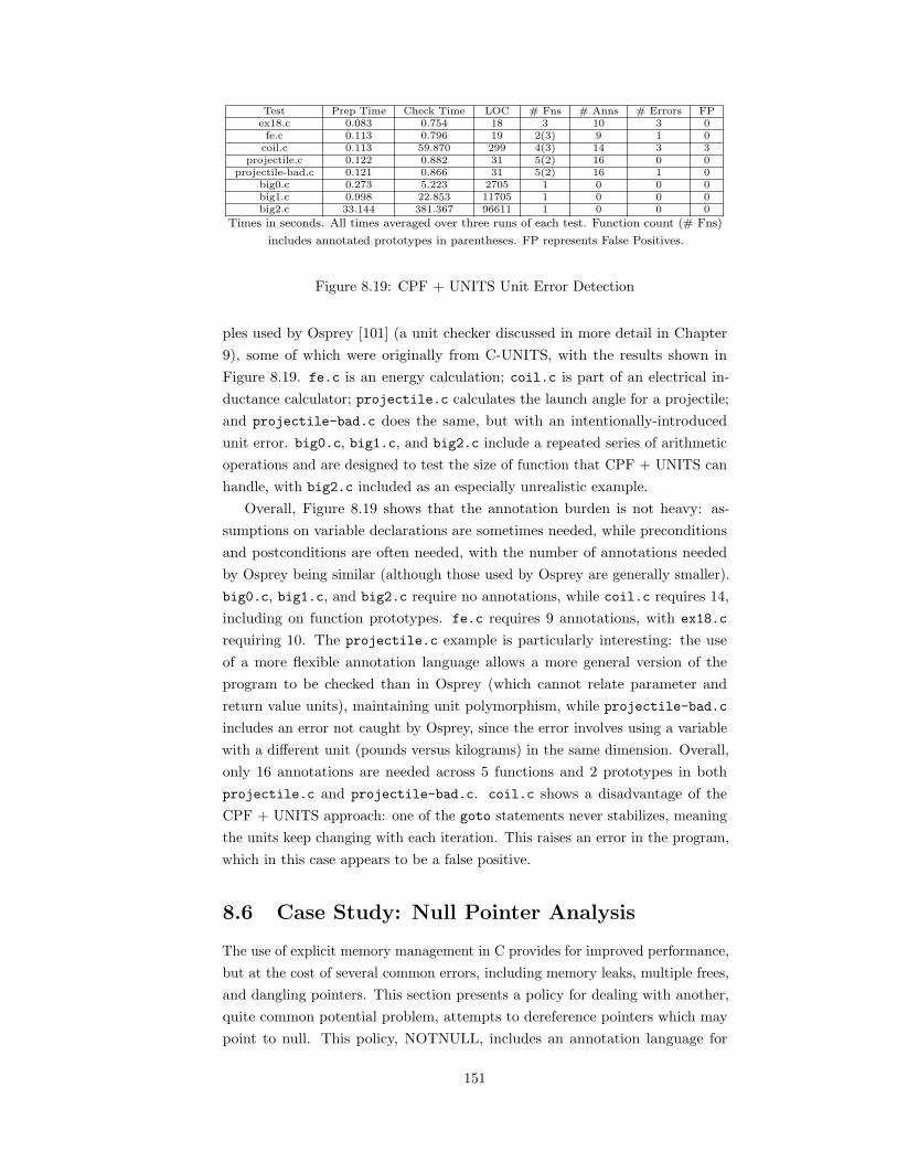
Test Prep Time Check Time LOC # Fns # Anns # Errors FPex18.c 0.083 0.754 18 3 10 3 0fe.c 0.113 0.796 19 2(3) 9 1 0
coil.c 0.113 59.870 299 4(3) 14 3 3projectile.c 0.122 0.882 31 5(2) 16 0 0
projectile-bad.c 0.121 0.866 31 5(2) 16 1 0big0.c 0.273 5.223 2705 1 0 0 0big1.c 0.998 22.853 11705 1 0 0 0big2.c 33.144 381.367 96611 1 0 0 0
Times in seconds. All times averaged over three runs of each test. Function count (# Fns)
includes annotated prototypes in parentheses. FP represents False Positives.
Figure 8.19: CPF + UNITS Unit Error Detection
ples used by Osprey [101] (a unit checker discussed in more detail in Chapter
9), some of which were originally from C-UNITS, with the results shown in
Figure 8.19. fe.c is an energy calculation; coil.c is part of an electrical in-
ductance calculator; projectile.c calculates the launch angle for a projectile;
and projectile-bad.c does the same, but with an intentionally-introduced
unit error. big0.c, big1.c, and big2.c include a repeated series of arithmetic
operations and are designed to test the size of function that CPF + UNITS can
handle, with big2.c included as an especially unrealistic example.
Overall, Figure 8.19 shows that the annotation burden is not heavy: as-
sumptions on variable declarations are sometimes needed, while preconditions
and postconditions are often needed, with the number of annotations needed
by Osprey being similar (although those used by Osprey are generally smaller).
big0.c, big1.c, and big2.c require no annotations, while coil.c requires 14,
including on function prototypes. fe.c requires 9 annotations, with ex18.c
requiring 10. The projectile.c example is particularly interesting: the use
of a more flexible annotation language allows a more general version of the
program to be checked than in Osprey (which cannot relate parameter and
return value units), maintaining unit polymorphism, while projectile-bad.c
includes an error not caught by Osprey, since the error involves using a variable
with a different unit (pounds versus kilograms) in the same dimension. Overall,
only 16 annotations are needed across 5 functions and 2 prototypes in both
projectile.c and projectile-bad.c. coil.c shows a disadvantage of the
CPF + UNITS approach: one of the goto statements never stabilizes, meaning
the units keep changing with each iteration. This raises an error in the program,
which in this case appears to be a false positive.
8.6 Case Study: Null Pointer Analysis
The use of explicit memory management in C provides for improved performance,
but at the cost of several common errors, including memory leaks, multiple frees,
and dangling pointers. This section presents a policy for dealing with another,
quite common potential problem, attempts to dereference pointers which may
point to null. This policy, NOTNULL, includes an annotation language for
151

Value V ::= $undefined | $defined V T
ValueType V T ::= $zero | $other | ptr L
Location L ::= $null | $notnull N
Figure 8.20: Not Null Policy: Policy Domain
specifying the “nullness” of pointers passed as function parameters and returned
as function results. The policy presented here is part of a larger policy, inspired
by the LCLint tool [49], that is currently under development.
The NOTNULL policy uses the default abstract values provided by CPF for
C objects such as pointers and structures. Scalars, which are not distinguished
by the policy, are all represented using a single abstract value, $scalar (an
exception is that 0 is recognized in some situations, since it serves as NULL in
C). For pointers that are null (i.e., that may be assigned null), a special memory
location, nullLoc, is used. Pointers that are not null (i.e., that must point to a
non-null memory location, albeit one that may contain garbage) point to actual,
non-null locations in the CPF C memory model. Two type annotations, $null
and $notnull, are provided to allow developers to encode this information,
with unannotated pointers considered $null. Annotation @nullity provides
additional support for stating or checking null properties of pointers and can be
used with logical connectives to form more complex expressions.
Given these abstract value and annotation definitions, the next step is to
define the policy semantics used during analysis. NOTNULL includes semantics
for expressions and for two kinds of statements: conditionals and loops. Also
included are semantics for pointer allocation, to ensure that null and notnull
pointers are initialized correctly. Some of the expression rules for pointer
dereferencing and assignment are shown in Figure 8.21. The dereferencing
〈k〉 ∗(ptr(L))llookup(L)
...〈/k〉 if L 6= nullLoc (8.22)
〈k〉 ∗(ptr(nullLoc))issueWarning(1, msg1,Env) y $fail
...〈/k〉 〈env〉Env〈/env〉 (8.23)
〈k〉 (ptr(nullLoc)) → XissueWarning(1, msg2,Env) y $fail
...〈/k〉 〈env〉Env〈/env〉 (8.24)
assignAllowed(ptr(nullLoc), L, (Env[ , L, , dsl(DSL) dcl(D) ])) = false
if isPointerDeclarator(D) and DSLContainsTAnn(DSL)
and @cpf (N) := getDSLTAnn(DSL) and isNNNotNull(NN) (8.25)
Figure 8.21: Not Null Policy: Pointer Dereferencing and Assignment
152

int *p = NULL;
if (p) {
... *p = 5; ... /* Should not cause a warning */
}
*p = 10; /* Should cause a warning */
Figure 8.22: Not Null Policy: Avoiding False Positives
operator, *, is strict, causing E in *E to be evaluated using heating and cooling
rules. Once E is evaluated, one of Rules (8.22) and (8.23) could apply. Rule
(8.22) handles the case where E evaluates to a pointer to location L, where
L is not nullLoc; in this case, we then look up the value at location L using
operation llookup. Rule (8.23) handles the case where the program attempts
to dereference a null pointer, and yields an error, issued using issueWarning,
with msg1 standing in for the issued warning message. Rule (8.24) defines this
same rule for pointers to structures, where field X is being accessed using the
-> operator (like p->x). Both failure cases return a special $fail value, which
is then propagated through other expressions without causing additional error
messages to be generated. Finally, Rule (8.25) is used during assignment to
determine if an assignment is allowed. This rule represents the failure case: when
assigning a value that is a null pointer, if the location being assigned to (L) is
declared to be a pointer (isPointerDeclarator), and if the declaration includes
a type annotation (DSLContainsTAnn, for declaration specifier list contains
type annotation), and if that annotation is $notnull (isNNNotNull), reject the
assignment. This catches attempts to assign null pointers to objects annotated
as not null.
For declarations, the pointer allocation semantics take account of the an-
notations on the pointer declaration, allocating storage for pointers annotated
as $notnull and assigning ptr(nullLoc) to pointers either not annotated or
specifically annotated as $null. The statement semantics for conditionals and
loops are also specialized for NOTNULL, specifically to account for specific
checks against null in the conditional or loop expression. If the expression is a
check to ensure that a pointer is not null, we can assume that it is not null in
the then branch or loop body, but that it is null in the else branch, eliminating
common false positives. An example code fragment is shown in Figure 8.22.
Here, the assignment of 5 to *p should not cause a warning to be issued, since
the user explicitly checks that p is not null, while the assignment of 10 to *p
should still cause a warning.
To allow for this scenario, the conditional logic is overridden, with specific
checks for different expression “patterns” common in null checking – the use
of just the pointer, like in if(p), or the use of a comparison against NULL, like
if(p != NULL) or if(NULL != p). In both patterns, the conditional body will
only be entered when the pointer is not null, so it is possible to assume this at
153

#include <stdlib.h>
int f($notnull int *v) {
int x,*p;
int $notnull *q;
p = (int*)malloc(sizeof(int));
q = v;
q = p;
*p = 5;
if (NULL != p) {
*p = 10;
x = *p;
free(p);
}
return x;
Figure 8.23: NotNull Example
the start of the body. Similar logic works for loops and if statements with else
branches. Note that we should not try to do the opposite, and assume a known
not null pointer is null after a check like if(!p), since this could lead to a false
positive.
Figure 8.23 shows an example of using the NOTNULL policy, with Figure
8.24 showing the analysis results. Function f takes a single parameter, an integer
pointer declared to be $notnull, and then declares three variables, an integer
x, a (potentially null) integer pointer p, and a $notnull integer pointer q. p is
allocated on line 5 using a call to malloc; since malloc returns null when no
memory is available, p could still point to null. Line 6 shows a correct assignment,
of one $notnull pointer to another. Line 7 generates an error, though, since it
could set q to null. Line 8 also generates an error, since p may still be null when
it is dereferenced. Line 9 contains an explicit check to see if p is null; since the
body is only executed when p is not null, we can assume this at the start of the
body, which is why lines 10 and 11 do not generate error messages.
8.7 Discussion
Chapters 7 and 8 presented policy frameworks, including an extended description
of the C Policy Framework. This section discusses some of the limitations of this
work; a comparison with other related work is provided in Chapter 9.
First, while the analysis semantics used as part of the policy framework are
often based on an existing semantics of the language, there is no automatic way
to either generate the analysis semantics or verify that the analysis semantics are
ERROR on line 7(1): Attempting to assign possibly null pointer to another
pointer annotated as definitely not null.
ERROR on line 8(1): Attempt to dereference possibly null pointer.
Figure 8.24: NotNull Sample Run
154

correct with regards to either the static or dynamic semantics of the language.
Work on this, in the context of generating environments for program verification
based on a dynamic semantics of the language, is ongoing.
Second, currently the focus has been on reuse of definitions of language
features across multiple policies within a language, instead of across policy
frameworks for different languages. This is in contrast to analysis domains,
which are intended to be reusable both across languages and across different
policies. The work on the module system is designed to support language feature
modules for analysis semantics as well, so we believe that it will be easier to
construct the language-specific parts of a policy framework from reusable pieces.
However, this area still needs further work.
Third, while the use of Maude provides many advantages, it can be an
unfamiliar platform for developing analysis policies for many potential users,
both in terms of the semantic techniques being used and the underlying (rewrite-
based) platform. One potential solution is to develop a layer on top of Maude for
developing analysis rules, with an automatic translation into Maude generating
the analysis semantics. This would still require some knowledge of Maude in
cases where something does not work as expected, but could provide a friendlier
environment both for those that are defining policies and for those reviewing
the policies to understand the analysis being performed.
155

Chapter 9
Related Work
Programming language semantics has been an active area of research since at
least the 1960s, with a number of different formalisms, including supporting
tools and techniques, defined between then and now. The first section in this
chapter, Section 9.1, compares a number of these formalisms with K. To maintain
focus, the formalisms presented here have been selected based either on their
popularity, on being especially relevant to the design goals of K and the work
presented in this thesis, or both. We especially focus on modularity, one of the
motivations for K and a driver for much of the work outlined in prior chapters;
tool support is also discussed briefly, with short evaluations and comparisons of
a number of popular tools built to work with language definitions.
Section 9.2 then focuses on program analysis, especially in the context of
systems that use either type or code annotations. The exception to this is a
comparison between the CPF UNITS policy and units analyses devised in other
frameworks, including solutions that make use of annotations, APIs for unit
manipulation, and language features specifically targeted at units (or features
which can easily be retargeted towards units). This provides related work and
comparative information both for the concept of policy frameworks as a whole,
and for one specific instantiation of a policy framework, the CPF UNITS policy,
that has driven much of the work on policy frameworks.
9.1 Programming Language Semantics
A number of techniques for defining the semantics of a programming language
have been developed over the years. The two most popular styles of semantics
for defining language features (instead of for verifying properties of programs)
have been operational semantics and denotational semantics. Various specific
instances of these styles are discussed below, including: structural operational
semantics, natural semantics, modular structural operational semantics, the
Scott-Strachey style of denotational semantics, and monadic semantics.
Although operational and denotational styles have been the most popular,
other semantics techniques, such as action semantics, rewriting logic seman-
tics, and abstract state machines, have also been used to define programming
languages. These are also discussed further below, along with a new style of
156

semantic definition, component-based semantics, that provides a way of struc-
turing modular language definitions to improve the reuse of individual language
features.
For each form of semantics discussed in this section, an attempt has been made
to provide enough information to motivate the comparison with K and to provide
intuition as to where tool support would be most helpful. For those interested in
learning more about the techniques discussed here, specific references that provide
more detailed explanations are cited as part of the discussion. Good overviews,
covering multiple semantic techniques, can be found elsewhere [176, 145, 155],
including detailed comparisons between these methods and both rewriting logic
semantics [172] and K [167].
9.1.1 Rewriting Logic Semantics
Rewriting logic, introduced in Chapter 2, provides a powerful computational logic
for representing deterministic, nondeterministic, and concurrent computation. As
a reminder, theories in rewriting logic are represented as triples R = (Σ, E, R),
made up of a signature Σ, a set of equations E, and a set of rules R. The
signature defines both the sorts of data in the theory, such as natural numbers
and strings, as well as the operations over that data (e.g., integer multiplication,
string concatenation)1. The equations, in conjunction with the rules of deduction
for equational logic, indicate which terms constructed over the signature are
provably equal. Rules, in conjunction with the rules of deduction for rewriting
logic, then determine transitions between equivalence classes of provably equal
terms, providing a way to indicate computational steps that do not lead to equal
states – for instance, in concurrent systems where the final result of a computation
is dependent not just on the actions taken by the various concurrently executing
parts of a system but also on the order in which the different parts actually
execute (including systems where two or more parts can execute at the same
time).
By creating the appropriate sorts, operations, equations, and rules, it is
possible to use rewriting logic to define various well-known models of concur-
rency [125, Chapter 5], such as Petri nets [159, 127], CHAM’s [64], and CCS
[132, 197]. Beyond this, it is also possible to define the semantics of program-
ming languages, including both standard sequential features of the language
(conditionals, comparison expressions) and concurrency features (threads, fu-
tures, synchronization). This area, dubbed rewriting logic semantics (or RLS)
[128, 129], encompasses much of the work in this thesis, including the creation of
formal language definitions for language prototyping and the use of an abstract
language semantics to define program analyses.
While much of the work on defining realistic languages has been focused on K
and its precursor, computation-based or continuation-based semantics, rewriting
1Additional information, such as an order relation over sorts for order-sorted signatures,may also be included in the signature; see Chapter 2 for more details.
157

logic semantics does not impose a specific definitional style. This has led to
a number of styles being developed over the years, including several based on
existing semantic formalisms, such as structural operational semantics or action
semantics. The remainder of this section focuses on these additional styles:
providing an overview of some related work, especially in areas relevant to the
other work on language semantics documented in this Chapter; discussing tool
support; and providing a comparison with the work on K.
Operational Semantics, Denotational Semantics, and the
Abstraction Dial
From the beginning [125], the connection of rewriting logic with operational
styles of language semantics, such as structural operational semantics (SOS)
[162] (described further below), has been recognized. Rules in an SOS definition
can be encoded naturally as conditional rules in rewriting logic. For instance, a
standard rule for addition in a language with state would be the following:
〈e1, ρ〉 → 〈e′1, ρ′〉
〈e1 + e2, ρ〉 → 〈e′1 + e2, ρ
′〉(EXP-PLUS-L)
Here, to add two numeric expressions, e1 and e2, one step of computation is
taken, changing e1 to e′1. e′1 could be a number, n, signifying that e1 has been
completely evaluated, or it could still be an expression with additional evaluation
steps remaining (for instance, if e1 is (2+(3+4)), one step of computation would
reduce this to (2 + 7)). Assuming the language being defined has side effects, ρ
changes to ρ′ to capture any changes to the state caused by the evaluation of e1.
The Maude version of this SOS rule would be:
crl < e1 + e2 , s > => < e1’ + e2 , s’ >
if < e1 , s > => < e1’ , s’ > .
Here, given the same initial expression, e1 + e2 is evaluated to e1’ + e2, with
s changing to s’ to capture any side effects caused by the evaluation of e1. One
difference between this rule and the SOS rule given above is that e1 can evaluate
directly to a number n even when the evaluation of e1 requires the application
of multiple steps in an SOS definition. Instead of needing to come back “to
the top” of the term being reduced each time, these additional steps can take
place inside the transition from < e1, s > to < e1’, s’ >. This is because
the rewrite relation is transitive, allowing multiple rewrite steps to be taken in
the transition from < e1, s > (it will be shown how this difference is remedied
below).
Rewriting logic also has a clear relationship with denotational semantics. By
encoding a sequential programming language as an equational theory (i.e., a
rewriting logic theory with no rewrite rules, R = (Σ, E, ∅)), such a language can
be given an algebraic denotational semantics [129], the preferred method being
158
through the use of initial algebra semantics [70]. In initial algebra semantics,
programs are represented as algebraic terms, which are members of (from Chapter
2) the term algebra TΣ. TΣ is initial in the class of all Σ-algebras, meaning there
is a unique homomorphism from TΣ to any other Σ-algebra. This homomorphism
can be seen as the meaning, or program evaluation, function, taking the syntax
of the program to its denotation, a value in one of the carriers of the target
algebra. In the case of equational logic, the denotation is actually an equivalence
class, made up of all terms which can be shown to be provably equal using the
stated axioms, given as equations, and the rules of equational deduction (given in
Chapter 2). For programs that terminate, the final value (i.e., 3) of the program
will be one of the terms contained in the equivalence class including the initial
program. A program is thus considered equivalent to its denotation.
For languages with nondeterminism, including concurrency, standard deno-
tational definitions use the concept of powerdomains [161, 177], which provide
a powerset-like construct for domains, capturing the fact that a program can
produce different answers based on differing underlying orders of execution. RLS
also supports a form of denotational semantics for languages with nondetermin-
ism using the initial model semantics of rewriting logic [125]. Given a rewriting
logic theory R = (Σ, E, R), the model of a program is given in the form of
a category. The objects of this category are members of TΣ/E , equivalence
classes of terms in TΣ formed using the equations E and the rules of equational
deduction. The morphisms of the category are also equivalence classes of terms,
but in this case proof terms based on the defined rewrite rules R, the rewriting
logic rules of logical deduction, and several additional axioms [125].
The fact that rewriting logic can naturally give both an operational and a
denotational semantics to the same language provides a way to unify both styles
of semantics within a single framework. One key to this is the ability to adjust
the level of abstractness of a language definition by using what has been termed
an abstraction dial [128, 129]. This dial works by adjusting the balance between
equations and rules in a language definition, with each program state defined as
an equivalence class of terms modulo the equations in the definition, and with
transitions between states defined using rules.
At one end of the dial, the highest, most abstract setting, the semantics of
a sequential language can be defined solely using equations. These equations
are generally confluent but, for most programming languages, not terminating,
since certain language features (infinite loops, recursive function calls, etc) may
cause programs to diverge. In this highly abstract semantics, a program P , all
configurations reached while evaluating P , and (for programs that terminate)
the final result of P are all part of the same equivalence class. As was discussed
above, this provides an algebraic denotational semantics for the language.
At the other end of the dial, the lowest, least abstract setting, it is possible
to provide a very concrete, fine-grained semantics by defining language features
159
solely with rules2. In this case, the individual computational steps defined by the
semantics lead to distinct configurations. This provides a traditional operational
view of the semantics, such as that given using structural operational semantics,
while still providing an initial model semantics for the language.
For most realistic languages, the proper setting is somewhere between the
two extremes. Most languages, such as Java, are mostly sequential, with many
of the language features definable using equations. However, most realistic
languages also have nondeterministic or concurrent language features, such as
thread synchronization or accesses to shared memory locations, which need to
be defined using rules.
This ability to turn the abstraction dial by adjusting the balance between
equations and rules can be leveraged to improve uses of the semantics. One
example is for program verification. Here, the semantics should be as abstract
as possible, reducing the size of the state space that then needs to be verified.
However, the semantics cannot be too abstract, since it is important to be
able to distinguish states which violate the properties being verified from those
that do not. Generally this leads to a definition like that mentioned above,
with the sequential features of a language defined using equations and the
nondeterministic or concurrent features of a language defined using rules. The
ability to distinguish different possible concurrent executions of a program then
provides a way to detect typical concurrency errors, such as deadlocks and
data races. An example showing the importance of the distinction between
rules and equations for verification was presented in Chapter 6 in the work on
shared memory pools for KOOL, where the ability to determine which memory
locations were local to a thread, with access modeled with equations, and which
memory locations where shared between threads, with access modeled using
rules, provided a significant decrease in the size of the state space, leading both
to faster verification times and to the ability to verify more complex programs.
Adjusting the abstraction dial also provides a method to model the computa-
tional granularity of a semantics. In a course-grained semantics, like the initial
algebra semantics, the initial program and the denotation of the program are
both in the same equivalence class, with the details of the computational steps
taken to reach the result of executing the program intentionally abstracted away.
In a fine-grained semantics, like a structural operational semantics, each step is
made intentionally distinct, providing a very concrete view of the computational
process used to reach a result. Adjusting the dial to intermediate settings pro-
vides a way to focus on specific parts of the semantics. One example was provided
above, with sequential features defined using equations and nondeterministic
features defined using rules. As a second example, one could provide a more
abstract definition of expressions, defining the semantics equationally, while
providing a more concrete semantics of control flow statements by defining them
2Even in this case, quite often auxiliary operations, such as those used to manipulate theconfiguration, are still defined using equations.
160
with rules. This gives the language designer a clear way to indicate what is
meant by a computational step.
However, one challenge in this is that straightforward encodings into rewriting
logic of other styles of semantics, such as structural operational semantics, do
not necessarily maintain the same computational granularity as the original
languages definitions. This was shown above in the discussion of operational
semantics, where the single rule for addition expressions given in rewriting logic
could trigger multiple computational steps (because of transitivity) instead of
just the one step taken in the SOS version of the rule. With reflexivity, a
rewriting logic rule could also take no computational steps, again not matching
the one taken by an SOS rule.
Research in this area has shown that is it possible to match the computational
granularity of a number of operational styles, including structural operational
semantics [126, 23, 172], natural semantics [172], modular structural operational
semantics [126, 23, 172], and reduction semantics [172] (i.e., context reduction).
For SOS and MSOS, this can be done by using special operators to control
reduction, ensuring that only one step can be taken at a time. The first proposed
solution [126, 23] made use of three types of configurations, shown below 3:
op <_,_> : Program Record -> Conf [ctor] .
op {_,_} : [Program] [Record] -> [Conf] [ctor] .
op [_,_] : [Program] [Record] -> [Conf] [ctor] .
The first, <_,_>, is the standard SOS-like configuration, used in the example
above. A rule starting and ending in this type of configuration is then used to
perform each step:
crl [step] : < P, R > => < P’, R’ > if { P, R } => [ P’, R’ ] .
In this rule, called step, a configuration containing a program P and a record
(state) R takes a step by first forming a new configuration with the same program
and record but with the second configuration operator, like { P, R }. The rules
in the semantics defining language features are then defined to use configurations
of this second form on the left hand side of the rule. When one of these rules
makes a computational step, the result is then stored inside a configuration
formed using the third configuration operator, like [ P’, R’ ]. The step rule
makes use of the values stored in this third kind of configuration, placing them
back into a configuration of the first form as the result of the step. The rewriting
logic rule for evaluating the left operand in an addition expression, revised to
use this format, would be:
crl { e1 + e2 , s } => [ e1’ + e2 , s’ ]
if { e1 , s } => [ e1’ , s’ ] .
3The brackets around the sort names in the second and third operators indicate that theseoperators works over kinds, instead of sorts, which can be seen here as error terms. The ctor
attribute indicates that these operators are constructors, used as building blocks to constructthe term being reduced.
161

The use of these three configuration operators allows the definition in rewrit-
ing logic to match the SOS definition by limiting the use of both transitivity
and reflexivity. With no rules defined to transition from configurations of the
form [ P , R ], transitivity is no longer an issue – additional rules cannot
automatically be applied. Also, since each step must go from a configuration of
the form { P , R } to a configuration of the form [ P’ , R’ ], reflexivity is
no longer an issue – changing from the second to the third form of configuration
can only occur when a step of computation is taken in a rule.
A later solution to this same problem [172], instead of using different configura-
tion operators to control rewriting, uses an operator that applies to configurations,
defined as:
op ._ : Config -> Config .
This operator, when applied to a configuration, allows the configuration to take
one step. This provides some additional flexibility, since it is then possible to
indicate that multiple steps should be taken by using the operator more than
once. For instance, given configuration C, . . C would indicate that two steps
should be taken. The solutions are otherwise equivalent. The same rule for
addition as was shown above, using this operator, would be:
crl . < e1 + e2 , s > => < e1’ + e2 , s’ >
if . < e1 , s > => < e1’ , s’ > .
It is important to note that the use of rewriting logic does not eliminate
the limitations of these various styles of semantics, discussed further below.
For instance, encoding SOS using rewriting logic still enforces an interleaving
semantics on concurrent computations, while encoding natural semantics using
rewriting logic does not remove the limitations that natural semantics has in
representing nondeterministic or diverging computations.
Modular Language Definitions
One important point not addressed in the above-mentioned work on rewriting
logic semantics is modularity – the ability to define each feature once and for all,
isolating it from changes caused by other features and allowing it to be reused
in different contexts. Inspired by the work on modular structural operational
semantics, also designed to meet this challenge, a modular definitional style
for rewriting logic semantics was created [126, 23]. This style has several key
features which lead to modular definitions, features which have some overlap
with those provided by K.
The first key feature is the use of record inheritance. The program configura-
tion is represented as a pair containing the current program and the program
state, called Record:
op <_,_> : Program Record -> Conf .
162
Record is an extensible record structure made up of a number of Fields, each
of which includes an Index (the name of the field) and a Component (the data
stored in the field), and where each Index is unique4:
fmod RECORD is
sorts Index Component Field Record .
subsort Field < Record .
op null : -> Record .
op _,_ : Record Record -> Record [assoc comm id: null] .
op _:_ : Index Component -> Field .
endfm
Any rules or equations (hereafter just rules unless the distinction is important) in
the language semantics that reference the Record include an additional variable,
PR, representing any parts of the record not mentioned in the rule.
The definition of Record as a set of fields, and the inclusion of PR in rules
that mention the record, both allow for record extensions as new features are
added without requiring one to revisit the definitions of existing rules. This is
because the PR variable present in the rules will automatically match any fields
not mentioned explicitly; the only rules that need to mention the fields explicitly
are those rules that access or update the information in the fields.
The second key feature is the use of abstract interfaces. Any sorts used to
represent key syntactic or semantic entities, such as statements or environments,
are defined abstractly, with a well defined interface (of operations) but no
concrete instances. The language definition maps entities to these abstract sorts
either through subsorting, making the concrete sort a subsort of the abstract
sort, or through coercions, defining an operator taking the concrete sort into the
abstract sort. This provides the same advantages as interfaces in languages such
as Java: the other rules deal with entities at the level of the interface, making
no commitments to the concrete representation, which can then be tailored to
the needs of the definition.
The third key feature is the use of certain rule formats which maintain
modularity. Rules should be of the form:
〈f(t1, ..., tn), u〉 → 〈t′, u′〉 if C
where f is a language feature, u and u′ are record expressions (including the
variable PR for the unmentioned part of the record), and t1...tn and t′ are terms
used in the semantics. In these rules, u, u′, and C should only mention basic
record syntax and operations defined as part of the abstract interfaces discussed
above. This allows the concrete representations to continue changing without
4The definition of Record presented here is slightly simplified: the uniqueness of each Index
is enforced in the actual definition by making a distinction between PreRecords and Records,and enforcing that only PreRecords with no duplicated Indexes are Records.
163

changing the rules, which would not be possible if rules mentioned the concrete
representations directly.
Using these techniques, a semantics-preserving translation from MSOS into
a modular rewriting logic semantics was defined [126]. This has been used in
the definition of a number of languages and in the creation of a tool for working
with MSOS definitions, the Maude MSOS tool [29]. This is discussed further
below with related work on MSOS.
Program Analysis and Verification
Along with definitions of the dynamic semantics of programming languages,
rewriting logic semantics has been used extensively for program analysis and
verification. One significant part of this work has involved the development of the
JavaFAN tool [51, 54]. JavaFAN includes two language definitions, one for the
Java language and one for Java bytecodes. It then leverages the tools provided
by Maude, including the breadth-first search capability and the LTL model
checker, to verify Java programs at both the source and bytecode levels. The
distinction between equations and rules is key for verification, since transitions
caused by features defined equationally do not increase the size of the state
space. By carefully choosing which features are defined using rules, and thus
keeping the state space as small as possible, JavaFAN achieved performance
competitive with purpose-build verification tools such as Java PathFinder [78].
Similar techniques have been used for some of the work described in this thesis,
including the work on improving the performance of model checking pure object
oriented languages [92] discussed in Chapter 6. Some additional work on reducing
the state space of concurrent systems defined using rewriting logic [52, 53] may
help to increase performance further, but it is not clear how easy it would be to
apply the techniques to K-style language definitions.
Another branch of the work on program analysis and verification has leveraged
techniques similar to those used in CPF, with analysis treated as program
execution over an abstract domain. A comparison of CPF with C-UNITS
[168], a tool developed using rewriting logic semantics for checking the unit (of
measurement) safety of C programs, is provided in Section 9.2.
Language Prototyping
The work on rewriting logic semantics has led to the definitions of a number of
other languages as rewriting logic theories. Included in this work are definitions
of: the ABEL hardware description language [106]; the BC calculator language
[23]; CCS [198, 23], a calculus for defining and reasoning about concurrent
systems; CIAO [182], the Calculus of Imperative Active Objects; Creol [102], an
experimental OO language for distributed objects; E-LOTOS [196], a specification
language; MSR [28, 180], a language for specifying cryptographic protocols; Orc
[10, 11], a language for the orchestration of distributed computations; PLAN
164

[181, 182], the Programming Language for Active Networks; PLEXIL [43, 164],
the Plan Execution Interchange Language, developed by NASA to support
autonomous spacecraft operations; and the π-calculus [186].
Along with definitions of languages, rewriting logic has provided an envi-
ronment for developing tools to work with definitions in different formalisms.
The Maude MSOS Tool [29] provides support for creating MSOS definitions
of language features which are then translated into rewriting logic; the Maude
Action Tool [40] provides similar support for definitions using action semantics.
Both of these tools are described further below in the sections on MSOS and
Action Semantics, respectively.
Some work, outside of that already mentioned above, has focused specifically
on the modularity of language definitions. For instance, work on defining Eden
[79], a parallel variant of Haskell, has focused on modularity in both the degree
of parallelism allowed and the scheduling algorithm chosen to select processes
for execution, allowing easy experimentation with these aspects of the language.
Comparison: As discussed above, rewriting logic semantics does not enforce a
particular definitional style, but instead supports a number of different styles,
including the continuation-based style that resulted in the development of K.
Because of this, comparisons on issues like the modularity of a definition or
the ability to support specific features must be based on the strengths and
weaknesses of the chosen formalism. For instance, a definition created using
an encoding of SOS into rewriting logic will have the same lack of modularity
as an SOS definition defined in another tool or on paper. Maude is used as
the underlying platform for the work discussed in this section, so ultimately K
(currently translated to Maude) and the other language definitions share the
same interpreter, breadth-first search, and model checking capabilities.
One area that does provide a point of comparison is modularity. One of
the motivations in the design of K was to improve the modularity of language
definitions. The work cited above on creating modular language definitions
[126, 23], introduced in 2004, takes a similar approach (referred to below as “the
RLS approach”) to that used in K, first used as part of the work on continuation-
based semantics in 2003 [166]. One distinction between the two approaches is
that, in the RLS approach, the current program is kept separate from the rest
of the program state, while in K it is just another state component, the k cell.
A second is that, in the RLS approach, the state is a flat record, while in K it is
often a hierarchy, with information grouped into different levels based on the
needs of the definition. While not explicitly disallowed in the RLS approach,
support for something similar to context transformers would be needed to allow
this hierarchical representation (to support changes in the hierarchy) while still
allowing language features to be defined once and for all. Finally, in the RLS
approach each state component can appear only once, while in K cells can be
repeated. The ability of K to nest configuration items, including the current
165

control context, inside other items, and to replicate configuration items, provides
a natural model for defining concurrent language features: each concurrent
thread of execution is in its own cell, with its own copy of state components such
as environments and locks held by the thread. The RLS approach seemingly
would require similar support to be added to define such features. A challenge
with both approaches is that modularity requires some discipline in the creation
of definitions, requiring either an experienced (with either K or RLS techniques)
language designer or careful planning.
Other differences between K and RLS can, for the purposes of this thesis, be
treated as mainly notational, with differences in the K notation then desugared
into standard RLS notation. Some of these features were added to handle
common language definition tasks that were often encountered while writing
RLS definitions in continuation-based style. One example is the use of the
contextual, K-style rules (and equations), where changes to a term are indicated
explicitly by underlining the parts of the term that change. One reason for this
notation was that it was often cumbersome to includes unchanged parts of the
term on both sides of the rule, with these unchanged parts often making up a
substantial part of the term, thus obscuring the important part of the rule – the
part of the term actually being changed.
Tool Support: Maude has been used as the main tool in the work on rewriting
logic semantics and K. A number of tools have been developed in Maude for
working with other styles of language definition, including the Maude MSOS
tool and the Maude Action Tool, both mentioned below. There is an ongoing
effort to create a Full Maude version of the K module system, similar to the
work on the Maude MSOS tool, as well as to extend support for working with K
definitions in Maude.
9.1.2 Operational Semantics
K takes an operational approach to defining programming languages, with rules
indicating transitions between configurations. This is the same approach taken
in two popular styles of operational semantics: structural operational semantics
[162], also referred to as small step semantics or transition semantics; and natural
semantics (NS) [105], also referred to as big step semantics.
In SOS, configurations include the program and, if needed, the program
state. The program state includes information such as the environment, the
store, definitions of classes and methods, etc. Semantic rules, of the form cl−→ c′,
are given to define the language semantics; c and c′ are configurations and l is an
optional label. The rules are defined to capture individual steps of computation,
such as a step of evaluation of a single operand in an arithmetic operation. As
an example, the rules for addition in a simple expression language without state
are shown below:
166
e1 → e′1
e1 + e2 → e′1 + e2
(EXP-PLUS-L)
e2 → e′2
n1 + e2 → n1 + e′2(EXP-PLUS-R)
n1 + n2 → n, where n is the sum of n1 and n2 (EXP-PLUS)
Note that the left operand, e1, is evaluated first, until it evaluates to a number,
n1. Once e1 evaluates to n1, e2 is evaluated to n2, enforcing a left to right
order of evaluation. Once both operands have been fully evaluated their sum is
computed, yielding n, the sum of n1 and n2.
In natural semantics [105], configurations are similar to SOS configurations.
However, the rules, instead of capturing an individual computational step, are
designed to completely evaluate the language feature being defined. An equivalent
rule to the above, given for natural semantics, is shown below:
e1 ⇓ n1 e2 ⇓ n2 n = n1 + n2
e1 + e2 ⇓ n(EXP-PLUS)
As in the SOS example, e1 evaluates to n1 and e2 evaluates to n2, with n then
calculated as the value of n1 + n2.
Comparison: SOS and NS both have several advantages over K. First, language
definitions given in either can be fairly mechanically turned into language
interpreters. This is especially true of NS, where the semantics can be represented
using recursive function calls and pattern matching. The natural model for K
interpreters, as term rewrite systems in Maude (or other systems that support
both associative and commutative matching), generally has slower performance,
which is one of the motivations behind still early work on generating high
performance interpreters and compilers from K definitions [86].
Second, SOS and NS both also tend to stay closer to the abstract syntax
of a language, providing a close mapping between syntax and semantics. K
definitions quite often introduce intermediate operations to represent different
steps of computation, which, if not done carefully, can make definitions harder
to understand. This has been remedied somewhat in K by using strictness
attributes, allowing a number of the rules used to evaluate individual operands
of a language construct to be generated automatically.
Third, although some work on using a K semantics as the basis for formal
proofs of both programs and programming language meta-theory has begun
[47, 170, 169], work on using operational techniques for these proofs is currently
more advanced, with a wider array of related work and techniques that can be
referenced by practitioners.
167

K also has several advantages over both SOS and NS. First, neither SOS nor
NS are modular, with changes to the configuration requiring changes to all rules
in the semantics, even those rules that just propagate the added configuration
items. For instance, if the simple expression language used in the SOS rules
shown above is extended with an environment to support the use of variables,
one would generally change the rules as follows:
〈e1, ρ〉 → 〈e′1, ρ〉
〈e1 + e2, ρ〉 → 〈e′1 + e2, ρ〉
(EXP-PLUS-L)
〈e2, ρ〉 → 〈e′2, ρ〉
〈n1 + e2, ρ〉 → 〈n1 + e′2, ρ〉(EXP-PLUS-R)
〈n1 + n2, ρ〉 → 〈n, ρ〉 where n = n1 + n2 (EXP-PLUS)
Unfortunately, the rules are not changed just when going from a semantics with
no program state to one with program state. Instead, rules are continually
adapted to include new state components, even if these components are not used
in the rules (as they were not above). This makes it much harder to use SOS
or NS to give a semantics to large languages, where it would be advantageous
to build the semantics in pieces. It also makes both frameworks poor choices
for language prototyping or for developing reusable language feature definitions,
since both would require the rules to be adapted (maybe repeatedly) to match
changes to the configuration.
Second, K supports a richer model of concurrency than either SOS or NS. SOS
supports an interleaving semantics, where a concurrent execution is represented as
multiple sequential executions, each of which is one of the possible interleavings of
computational steps that could be taken by the concurrently-executing processes.
The model supported by NS is simpler: given that each rule in the semantics is
atomic, taking the language construct to its value in one “big step”, only one
of the concurrent paths is chosen, with interleaving not allowed (e.g., given a
number of threads, each thread would run to completion before the next could
start, with no communication between the two allowed except when one yields a
result that another then uses).
Some research has tried to work around this by adding a trace relation to
natural semantics [134]. This allows some concurrent features to be captured,
with a main thread that computes a value and worker threads that can com-
municate with the main thread asynchronously, influencing the final computed
value. However, this model is still limited: interleavings are lost, since only the
computed value is deemed important, not the process used to compute this value;
worker threads cannot communicate with one another; and it is still difficult
to represent situations such as divergence and deadlock (especially of the main
thread). Because of this, concurrent languages defined in natural semantics
168

“escape” to some other form of semantics when defining the concurrency fea-
tures [13, 187]. The author is unaware of any real concurrent languages defined
completely using natural semantics.
In contrast to both SOS and NS, K supports true concurrency [138, 137, 125],
which allows defining semantic rules where multiple concurrent processes take
computational steps at the same time. This provides a semantics closer to the
actual behavior of programming languages than an interleaving-based semantics,
especially with the increasing use of multi-core, parallel, and distributed systems
that have actual concurrency, instead of just systems where concurrency is
simulated (for instance, by thread scheduling).
Third, both SOS and NS have difficulty representing language features that
involve complex control flow. Features like exceptions generally require either
modifying the configuration or passing program values representing the control
flow event (like a thrown value), with special versions of rules needed to either
check this flag or propagate this event; some features, like continuations, have no
natural definition in either SOS or NS, but instead require defining the semantics
of both the language and at least part of the evaluation mechanism (i.e., defining
a runtime that supports continuations, versus defining the language directly).
This has led to the use of conventions in actual language definitions, such as those
used in the definition of Standard ML to handle exceptions [133]. By contrast,
these features can be modeled easily in K because of the explicit representation
of the current computation as a term, which allows computations to be stored,
restored later, or constructed as necessary.
Tool Support: A classic example of a semantics-based language environment
is Centaur [22], an ambitious project which allowed languages to be defined
formally, with the formal definition then used to generate a suite of graphical
language-support tools. Language semantics were defined using natural semantics
in a Prolog-like language named TYPOL; this TYPOL definition was then
converted into Prolog, allowing programs to be evaluated in the semantics using
logical reasoning. Centaur inherits the benefits and faults of natural semantics,
including the lack of modularity, making it difficult to create reusable definitions
of language features. One goal of our work on K is to create tools like those
provided by Centaur; the K tool support currently focuses on program execution
and analysis, instead of generating tools, such as editors and debuggers, which
would be useful for language designers and language users.
Two other tools used for operational definitions are LETOS [77] and RML
[160]. LETOS provides a lightweight language development environment for
operational semantics definitions in a literate style reminiscent of literate Haskell,
with LATEX formatted documentation and specially demarcated blocks contain-
ing language definition rules. These rules can be translated to allow program
execution in either Miranda or Haskell. LETOS can also be used for denota-
tional definitions, but with reduced functionality, mainly losing the ability to
169

visualize rule application. RML is focused mainly on compiling natural seman-
tics definitions to generate efficient implementations, but lacks features such
as visualization of rule application available in some other tools. Both tools
again inherit the limitations of their formalisms, but both also provide an ability
currently lacking in K: the ability to generate interpreters in languages which
can then be compiled for performance.
The Ott system [173] is described as a meta-language and tool designed
to support the “working semanticist”. The meta-language allows definitions
of languages to be specified as inductive relations, with special support for
binding and substitution. Tool support includes the ability to include LATEX
documentation in definitions, check definitions to ensure they are consistent (in
the words of the authors, to “sanity-check” the definitions), and generate language
definitions and proof tasks for a number of commonly-used theorem provers: Coq,
HOL, Isabelle, and Twelf. Ott has been used to define a handful of languages
and language calculi, including a significant subset of OCaml and the Lightweight
Java Module System [185]. Ott’s strongest aspect is its focus on theorem proving;
the lack of executability, and the reliance on non-modular language definition
techniques, would make it difficult to use as a language design environment
and would make it hard to reuse parts of language definitions, something that
could be quite useful in a theorem proving context. With these limitations, it
is unclear how easy it will be to define an entire language in Ott or to extend
existing language definitions as languages evolve over time.
Reduction Semantics
Reduction semantics [57] was designed to provide better support for defining
control-intensive features in (especially imperative, but also functional) program-
ming languages [56]. This is done by defining reduction contexts, which are
places in a program where computation can occur; and reduction rules, which
determine steps of program evaluation. Support for control-intensive features is
provided by allowing the rules to access not just the part of the program inside
the reduction context “hole” (i.e., the redex), but also the surrounding context
of the computation, which can be saved, modified, or replaced as needed. The
ability to manipulate the computational context, and the focus on reducing terms
in a context, gives rise to two other common names for this style of semantics:
context reduction, and context-sensitive term rewriting.
Comparison: Context reduction maintains some of the same advantages of SOS
over K, such as the close relationship between the syntax and semantics, while
also providing improved support for defining control-intensive features. Work on
using context reduction for language meta-theory proofs, such as proofs of type
soundness, is also more advanced [207] than the equivalent research using K [47].
Finally, the ability to abstract the context in which a rule applies provides some
170
of the same modularity benefits as the use of matching over multisets in K or
the use of labeled configuration items in MSOS (discussed below), insulating
rules from changes not related to the referenced parts of the configuration.
At the same time, context reduction also has some limitations, both compared
to other operational styles and to K. First, the execution model for context
reduction definitions is quite complex, with the system needing to find a redex
at each step, requiring the entire term tree to be searched. Certain techniques,
such as refocusing [39], help to alleviate this, but only work in restricted cases.
For instance, refocusing requires that the unique decomposition property holds,
which states that any non-value term t can be uniquely decomposed as t = C[r],
where C is the context and r is a potential redex. However, this property only
holds in deterministic languages, since it states that there is only one part of
the program that can be evaluated (i.e., run) at any one point in time.
Second, reduction semantics only supports an interleaving semantics for
defining concurrent language features, giving it a more limited concurrency
model than the true concurrency model supported by K and rewriting logic.
Finally, although the representation of context provides some modularity, changes
in context, such as adding new context “groupings” to represent threads, would
still require changes to rules that referenced the prior context layout. This limits
the ability to reuse defined language features and to extend existing languages
with new language features, operations directly supported using the modularity
features (context transformers, the module system) of K.
Tool Support: PLT-Redex [123] is a graphical environment, built on top of
PLT-Scheme and the DrScheme interface, that allows for the development of
language definitions using context reduction. PLT-Redex includes several useful
features which have served as an inspiration as we have designed tool support
for K, including the ability to visualize reduction steps graphically, design test
suites for semantic features, and generate some forms of documentation for the
semantics.
However, PLT-Redex does have some limitations which could make it difficult
to develop and experiment with large language definitions. One important
limitation is performance: language definitions run very slowly, and often have
a large resource footprint. This can make running even small programs very
time consuming. Part of this is due to the lack of definitional constructs, like
sets, commonly used in K definitions (all lookups become list lookups in PLT-
Redex). Another is that language definitions make use of Scheme, requiring an
understanding of the Scheme semantics to get a full, formal understanding of
the semantics being defined, a problem similar to that mentioned below with
semantics-based interpreters5. On the other hand, PLT-Redex has found a
5PLT-Redex could actually be considered to be a semantics-based interpreter, but, since itprovides a number of constructs for language definition that sit on top of Scheme, it is usefulto look at it separately.
171

number of applications in language design, spawning a local workshop and a
book [55] with a number of case studies.
Modular Structural Operational Semantics
Although SOS definitions have many benefits, one of the key problems, mentioned
above, is that the definitions are not modular, making it difficult to initially
construct and then maintain definitions of realistic programming languages. One
attempt to solve this problem is Modular Structural Operational Semantics
[144, 146], or MSOS. The key difference between MSOS and SOS is in the
use of labels on rules. In SOS, labels are generally not used in definitions of
programming language features, but are instead used for giving semantics to
other systems, such as process calculi. This has been exploited in MSOS [147]
by using the rarely used labels to hold all information from the configuration
except for the current program. Using certain notational conventions, it is then
possible to define rules that only refer to the parts of the state, given in the rule
label, that they need, with the others elided. This ability to not mention parts
of the state that are not used is key to ensuring modularity – as long as only the
unused part of the state changes, the rules given in the semantics do not need to
change.
For example, the following rules give the MSOS definition of the plus expres-
sion, given above for both SOS (with and without state) and NS (just without
state):
e1{...}−−−→ e′1
e1 + e2{...}−−−→ e′1 + e2
(EXP-PLUS-L)
e2{...}−−−→ e′2
n1 + e2{...}−−−→ n1 + e′2
(EXP-PLUS-R)
n1 + n2{–}−−→ n, where n = n1 + n2 (EXP-PLUS)
Again, note that most of the information in the configuration is gone (or,
more accurately, hidden in the label)– these rules now look very close to those
given originally in SOS for a language with no state. The “...” over each arrow
represents unmentioned parts of the state, with “...” representing the same state
both above and below the line dividing the premise and conclusion of the rule.
This can be read as “if the transition from e1 to e′1 (for instance) makes some
change in the state, then the transition from e1 + e2 to e′1 + e2 makes the same
change in the state”. Because individual parts of the state are not named, and
because changes to this state are still propagated, the state itself can change
(say, when adding environments or updatable stores with assignment expressions)
without requiring any changes to these rules.
172

In cases where the state should not be changed by a rule, it is possible to
note this using “–”, instead of ..., over the arrow. Technically, this makes the
label unobservable, so the rule can make no changes to the state that would be
visible elsewhere. Using “–” is obligatory for axioms, to ensure that they do not
allow arbitrary changes to the state. It is also possible to use “–” for rules with
premises, which can be important in some contexts (such as for some proofs),
but which could also limit reuse of the rule, as it could no longer propagate
changes to the state not mentioned directly in the rule. An example with “–” is
shown above in the axiom given for plus expressions.
When the state is needed, the state components in the label are treated
similarly to components of an ML-like record, allowing them to be accessed by
name. A rule for name lookup could be:
x{Env=env ,–}−−−−−−−−−→ env(x) (LOOKUP)
To represent changes from the initial information in the state, components of
the state can be given with a prime, representing the state at the end of the rule.
For instance, a rule in an imperative language for assignment, where the state
contains an environment (mapping names to locations) and a store (mapping
locations to values) would be:
x := v{Env=env ,Store=mem,Store′=mem[env(x)←v],–}−−−−−−−−−−−−−−−−−−−−−−−−−−−−−−−−−→ skip (ASSIGN)
where mem[env(x) ← v] is the original value of mem but with the value at
location env(x) replaced with v.
One shortcoming of MSOS is that the rules, with configurations given on
labels, look more complex, or at least unfamiliar, to those familiar with standard
SOS rules. This has been addressed in Implicitly-Modular SOS (I-MSOS) [153],
which allows the use of the more familiar SOS notation when defining rules.
I-MSOS rules are then automatically translated into MSOS rules, providing both
the simplicity of SOS and the added modularity of MSOS. An example, drawn
from a recent paper [152], provides an example of the rules used to evaluate a
let construct:
ρ ⊢ E → E′
D → D′
(let D in E)→ (let D′ in E)(LET-DECL)
ρ[ρ1] ⊢ E → E′
ρ ⊢ (let ρ1 in E)→ (let ρ1 in E′)(LET-EXP)
(let ρ1 in V )→ V (LET-FINAL)
The shading in the definition of the relation specifies which parts of the
definition represent the state (ρ ⊢) versus which parts represent the syntax
173

(E → E′). It also provides the information needed to transform the rules into
equivalent MSOS rules. Note that, of the three rules, only the second mentions
ρ, making it implicit in the other two.
Comparison: MSOS and I-MSOS are both extensions of SOS targeting SOS’s
modularity problems. Thus, they maintain the advantages of SOS over K
(except, perhaps, in program proofs and language meta-proofs, where MSOS and
I-MSOS have not been as widely used), while also addressing one of the major
disadvantages, modularity. MSOS and I-MSOS provide the same modularity as
K with context transformers, allowing rules to continue being used unchanged
as a language evolves, and also allowing rules to be reused across languages.
Since MSOS and I-MSOS (from here just MSOS, unless the distinction is im-
portant) are built on top of SOS, they also share some of the same disadvantages.
MSOS uses an interleaving semantics, versus the true concurrency model used
in K, and continues to have some of the same challenges in defining control-flow
intensive features, especially call/cc. It is, however, now much easier to add
support for configuration “flags”, such as a flag indicating that a halt command
has executed, since only the top-level rule (such as statement sequencing) and
the rule that sets the flag need to be aware of this.
A final distinction is that the configuration itself is much more dynamic in K
than in MSOS: it is possible to rename cells or add new cells in rules where, to
the authors knowledge, it is not possible to do something similar in MSOS. While
not essential in many programming languages, this can be useful in the definition
of certain features. For instance, CPF, described in Chapter 8, regularly adds
and removes cells during program analysis, based on the needs of the rules in the
analysis semantics. As another example, KOOL, described in Chapter 3, renames
the cell holding the store during garbage collection (described in Chapter 6),
indicating that none of the rules that match the store can apply. This makes
it easier to guarantee that the mutator and the collector do not conflict. Also,
most concurrent languages defined in K create new cells to represent new threads
(and their contents). This dynamism comes with a potential cost: verifying
the correctness of both language features and programs in defined languages
may be harder with a dynamic configuration, and would make formalization
using standard techniques (such as giving the configuration as a tuple) more
challenging.
Tool Support: There have also been several tool support platforms introduced
for MSOS during its development. One method of executing MSOS definitions
that has been explored is to use Prolog [148], with evaluation then based on
Prolog reasoning. Another alternative, the Maude MSOS tool [29], is an extension
to Maude built using Full Maude [44, 35]. The Maude MSOS tool allows MSOS-
specific Maude modules to be defined using MSDF, the modular SOS definition
174

formalism. These modules are then automatically translated into standard
rewriting logic system modules using a semantics-preserving transformation [126]
from MSOS to rewriting logic, allowing MSOS rules to be used for program
execution and analysis. The K module system provides similar functionality,
leveraging the K tool kit to provide a translation into Maude while also providing
an additional layer of abstraction, allowing use of a friendlier syntax for defining
modules as well as syntactic sugar for a number of common scenarios, sort
aliasing and variable prefixes being just two examples. This additional layer
of abstraction has proven quite handy in working around some of the parsing
restrictions in Maude: for instance, because of the way that rules and equations
are parsed, variable prefixes are quite challenging to add directly into the Full
Maude version of the module system that is currently being built, something
the author unfortunately discovered in the middle of the implementation.
The Maude MSOS tool not only supports standard monolithic definitions,
but also supports the new component-based style of definition. This definitional
style, along with other work on tool support for MSOS (which also supports this
style), is discussed below.
9.1.3 Denotational Semantics
In denotational semantics, the semantics of a language construct is given as
a function which maps the construct to its denotation, a mathematical value
that provides the meaning of the construct. In the Scott-Strachey approach to
denotational semantics [183, 171, 141], semantic functions map each language
construct to a value in a Scott domain [73], formed using both primitive values
(e.g., natural numbers) and constructs such as function spaces, products, and
sums. The semantics are compositional, meaning that the semantics of a feature
is defined in terms of the semantics of its subfeatures.
As mentioned above, K takes a more operational approach to language
semantics. However, K definitions also have a clear denotational semantics. Like
definitions in rewriting logic semantics, K definitions with only equations have
an initial algebra semantics, while K definitions with rules have an initial model
semantics. Further details are provided earlier in this chapter, in the comparison
between rewriting logic semantics and denotational semantics.
Comparison: The standard techniques for denotational semantics provide
several advantages. The close link between denotational semantics and functional
languages, especially pure functional languages such as Haskell, provides a natural
way to “implement” denotational definitions, while also allowing techniques
developed for semantics (like monads, discussed below) to filter into standard
practice in the functional language community. The abstraction gained from using
denotational definitions has also proven to be valuable for better understanding
and reasoning about programs and programming language definitions. This can
be seen in work such as the LOOP project [100, 188], which used a denotational
175
definition of the JavaCard version of Java as a basis for verifying the correctness
of JavaCard applications. Finally, the use of lambda notation in the definitions
of languages provides a standard base language for describing and comparing
language features.
There are also some disadvantages to these techniques which are addressed
by K using the underlying algebraic denotational semantics and initial model
semantics of rewriting logic. Initial algebra semantics provides a more natural
mapping from the abstract syntax of a program to the semantics, without a
need to encode language semantics into potentially complex lambda terms. Also,
the first-order nature of the definitions can occasionally provide more insight,
since operations provided by the semantics are not given in terms of features of
the underlying notation which may themselves have complex definitions (such
as variable binding and substitution)6. Finally, rewriting logic provides better
support for reasoning about and representing concurrency, without the need to
use constructs such as powerdomains (for which, to this author’s knowledge,
there are still several competing definitions).
Monads
A well-known limitation of denotation semantics is that, like the definitions of
language features in structural operational semantics, denotational definitions of
language features are not modular [141]. The use of traditional lambda notation
to define the semantics imposes the same restrictions found in pure functional
languages: any state, such as (in semantics definitions) environments, stores,
etc, needs to be threaded through the defining functions. When new language
features are added that require extensions to the configuration, all existing rules
need to be modified, even those that do not use the new parts of the configuration,
to ensure the entire configuration is propagated.
One proposed solution for improving the modularity of denotational defi-
nitions is monads [135, 136]. Although quite different from the solution used
in MSOS, there are also some similarities. In MSOS, configuration items are
given as part of the labels on transitions, providing what can be viewed as an
extensible record structure for storing configuration information. Using monads,
this configuration information is instead stored inside a monad which represents
a computation. The semantic functions return computations, not values, allowing
computations to be threaded through the semantic rules. At the same time,
the monad itself is treated like an abstract data type, with an interface that
knows about the configuration items stored inside and exposes them through a
defined (functional) interface. In essence, instead of threading the configuration
through the functions in pieces, it is automatically carried inside the computation,
allowing rules that know about the monad to be defined without then needing
6Note that this could be seen as a disadvantage by some, since this can require moreformalization effort.
176
to be changed when the internals of the monad change (assuming the interface
does not also change).
Although introduced as a method to modularize denotational definitions,
monads were popularized when first applied in a more practical setting: represent-
ing state in purely functional programming languages such as Haskell, especially
in the context of language interpreters and compilers [200, 201]. This initial
work provided a way to localize stateful operations, but did not provide an easy
way to either combine different features or “plug in” features without changing
the surrounding code. Subsequent work, [111, 103, 179, 116, 115], while often
maintaining a focus on interpreters, also focused on methods of programmatically
combining monads using monad transformers, ensuring that the resulting monad
(the combination of the input monads) preserved the required mathematical
properties. The result of one line of this work is Modular Monadic Semantics
[115], which structures the semantics of a language by defining them in terms of
a number of predefined monads that provide common language building blocks
(stores, continuations, etc).
Another line of work has focused more on the theory surrounding monads,
although it has also (in many cases) maintained a practical focus, with imple-
mentations of the concepts provided in functional languages such as Scheme,
Haskell, or Gopher. This includes work on language development environments
such as Semantic Lego [48], which focused on combining monads for different
language features using a concept called stratification, allowing monads to be
combined by “building them up” in the desired order, instead of “lifting” them
through other monads with monad transformers. Even with stratification finding
general-purpose ways to combine monads has still been problematic; some recent
work has focused on defining the combination of two monads as their coproduct
[119], which appears to work in most cases except for continuations, which are
problematic for many of the proposed methods.
Finally, along with some of the work mentioned above [115], some additional
work on monads has focused on issues that are more specific to compilers
[76, 174, 175], such as the need to divide compilation up into different stages
(represented by a monad for each stage).
Comparison: Monadic semantics provides a structuring mechanism for denota-
tional semantics, so it shares many of the same benefits and limitations with
standard denotational semantics definitions. The main distinction is that monads
provide a way to make languages more modular, with individual features designed
around monads that contain the needed state. Monads have also been highly
successful as a method for structuring functional programs, leading to a number
of techniques for building language interpreters, using monads, in functional
programming languages (especially Haskell and its variants and Scheme).
In comparison with K, there are also several limitations of monadic semantics.
The main limitation, outside of those already mentioned for denotational seman-
177

tics, is that there is no truly modular way to combine different monads using
monad transformers. In some cases, there is no automatic way to meaningfully
combine modules. Instead, transformers sometimes must be written by hand,
ensuring that the correct monad laws hold (especially problematic, as usual, are
continuations). Monad composition is also order dependent, meaning that a
different semantics could be given to a language based on the order in which the
underlying monads are combined. Since the number of transformer application
orderings is quadratic in the number of monads being combined, this can quickly
grow unwieldy in large language definitions. It also seems likely that, in some
cases, it would not be possible to find an ordering that would satisfy all the
needs of the language.
These problems are dealt with in K by using one global transformation
over all the rules in the language once the rules are chosen and the language
configuration is assembled, versus using a series of individual transformations
as the language is built. This transformation should be able to build only one
proper configuration; if it can build more that one, the rules are ambiguous, and
the user is tasked with fixing the rules to ensure a unique final configuration can
be found.
Tool Support: Most of the work discussed above was conducted in the context
of creating modular interpreters, leading to several tools designed for this purpose.
Some of the most notable include: interpreters based on pseudo-monads, written
in Haskell [179]; monadic interpreters and compilers, written in Gopher (and, in
the latter case, targeting Standard ML) [116, 115]; monadic interpreters written
using Scheme [48]; and compilers built with explicit compiler stages, represented
as monads [76, 174, 175].
An advantage of these tools over the current tool support for K is the use of
more typical functional languages for implementations, which provides a more
familiar environment and features such as compilation. A disadvantage, already
mentioned above, is that the specification of the semantics of one language
using another can mask the actual complexity of certain language features, and
can require the language designer to understand both the defined and defining
languages to fully understand the language definition. Otherwise, the benefits
and limitations are as described above.
9.1.4 Action Semantics
Action semantics [142] was defined with the goal of “allow[ing] useful semantic
descriptions of realistic programming languages” [142, page xv]. It includes
several major differences from standard operational and denotational styles of
semantics, while still maintaining some of the signature features (definitions
are given using an operational style, but are also compositional and map to
denotations, albeit not given as values in Scott domains).
178

First, instead of using lambda notation (like denotational definitions), which
can become quite complicated as language definitions become larger, more com-
plex, and more realistic, action semantics uses action notation. Action notation
defines a number of primitive actions (that perform computation) and action
combinators (that combine smaller computations into larger computations), as
well as methods for defining data and yielders, entities that can be evaluated to
yield data. Although formally defined, action notation uses English instead of
mathematical notation, making language definitions more readable.
Second, action semantics has improved support for modularity over standard
operational and denotational semantics, giving it capabilities which appear
similar to those of monads. Items in the configuration are modified by actions
but propagate, for the most part, behind the scenes, using special actions to (for
instance) allocate and update storage cells. Actions are separated into facets,
each of which deals with a different kind of information (transient data, bindings,
control flow, etc)7. Parts of a definition that work on one facet then do not need
to worry about changes to other aspects of the definition. Much like MSOS,
monads, or K, this protects definitions of language features from changes in
unused parts of the state, allowing languages to evolve or features to be reused
in other languages.
Third, action semantics includes improved support for concurrency over
what is provided with denotational semantics [143]. This includes constructs to
represent nondeterministic choices in the semantics (including from intentionally
underdefined language features) as well as an asynchronous model of concurrency
and distribution similar to that found in Actors [7]. This model supports true
concurrency, with different agents making progress at overlapping times.
Originally action semantics was defined using a non-standard variant of
SOS. The current definition instead uses MSOS, providing a cleaner underlying
semantics and an opportunity to more easily extend action notation with new
constructs if needed. Alternative definitions have been based around monads
(described below as modular monadic action semantics) and ASMs (with an
implementation using a tool and technique called Montages, presented below as
part of the discussion around ASMs).
More recent work on action semantics has focused on defining languages
using a number of small (per-feature) modules. This work is discussed below
under component-based semantics.
Comparison: Conceptually, there are some similarities between action se-
mantics and K. In K, computations are driven by a number of provided and
user-defined operators which work on the computation and other parts of the
configuration. Action notation provides a similar language for action semantics,
with semantics defined in terms of actions instead of K operations. In both K and
7Some actions cover more than one facet.
179

action semantics there is no need to reference unused parts of the configuration,
and both support true concurrency.
One difference between action semantics and K involves the use of kernel and
derived operations. In K, the semantics of both kernel and derived operations
is given in K notation, and, although a boundary between the two could be
maintained, in practice it is not. In action semantics, kernel operations are defined
directly in the underlying (now MSOS) semantics, while derived operations are
defined in terms of other already-defined action semantics operations. This
makes the boundary between the two more distinct.
Both approaches have disadvantages and advantages. In action semantics, it
is harder to add new features not supported by the notation, since one needs to
“escape” to MSOS to do this. However, the focus on defining new operations in
terms of existing operations aids in understanding and reusing defined features
and in comparing different definitions. In K, the ability to easily add new
operations provides a straightforward way to support new language features, but
the unwise use of this support can lead to redundant and harder to understand
feature definitions. One purpose of the K module system is to provide a more
direct way to reuse already defined features, introducing more discipline into the
process of K language design.
Beyond this there are several other interesting points of comparison. First, in
action semantics, the division of semantic features into different facets provides
a separation of concerns in the semantics that does not exist in K and would be
beneficial. Second, like in MSOS, it is not possible to define the semantics of
call/cc in action semantics without defining the language semantics to also include
the semantics of the underlying runtime. Third, action semantics supports some
forms of concurrency – specifically, concurrency that can be modeled as agents
communicating using asynchronous messages – but not others, including standard
threading models with shared memory and threads that can be interrupted and
resume execution later. K can naturally define these features.
Tools: ASD [195], the Action Semantic Description tools, provides an environ-
ment for working with action semantics descriptions. Included are tools for
parsing descriptions, syntax-directed editing, checking for well-formedness, and
transforming programs into equivalent programs using action notation in place
of the original language constructs. ASD is written using the ASF+SDF Meta-
Environment [192], with ASD definitions translated into equivalent ASF+SDF
constructs. ASD does not appear to support running programs using action
notation, but instead is focused on working with language definitions. This is
similar to the work on the K module system, although ASD supports features we
are still adding (such as improved well-formedness checking of definitions, which
is only partial at this point since much of the parsing of rules and equations is
performed in Maude).
Another tool, the Maude Action Tool [40], is an action semantics-driven
180
interpreter. It accepts a description of a language, defined in action semantics,
and a program in the described language. The language description is translated
from action notation into Maude notation, which is then used to “desugar” the
input program into an equivalent program using action notation in place of
the syntax of the language. Another transformation is used to transform the
underlying MSOS semantics of action semantics into an equivalent rewriting
logic theory (a system module). Using this rewriting logic theory, the desugared
programs can then be executed in Maude. It would also be possible to apply
Maude’s analysis and verification features (model checking, state space search),
although it is not clear if this has yet been tried. This translation is similar in
approach to the current K tools, although in K, instead of desugaring a program
into semantic constructs, the semantics are built over the abstract language
syntax.
There are several other notable tools for working with or interpreting programs
using action semantics definitions. One [12] uses Montages [113] (discussed below
with ASMs) to define the underlying semantics of action semantics, providing a
semantics-based interpreter for running, debugging, and visualizing programs.
Another tool, the Action Environment [191, 189, 190], is discussed below in
the section on component-based semantics. Finally, Modular Monadic Action
Semantics [203], which uses monads to implement the base semantics of action
semantics and provides a monadic interpreter, is discussed later in this section.
Action semantics has also been a popular target for research on semantics-
driven compiler generation. One example is OASIS [157], which takes a semantic
description written in Scheme and generates a Perl-based compiler, which then
generates executable code for SPARC processors. Another is Actress [25], which
generates an action semantics-based compiler that then compiles source programs
into C. Work on generating high-performance interpreters and compilers using
K definitions is still in early stages of development [86].
Modular Monadic Action Semantics
One limitation of the initial version of action semantics [142] was that the
underlying semantics were based on a non-modular SOS definition, making it
challenging to extend action semantics with new facets or new basic constructs.
Another was that the theory for reasoning about programming languages defined
using action semantics, as well as reasoning about programs based on an action
semantics of the underlying language, had not been (and, to the author’s
knowledge, still has not been) a focus of the research, making this kind of
reasoning challenging.
One solution to this problem was to replace the underlying operational (SOS)
definition of action semantics with a Modular Monadic Semantics (as discussed
above), leading to a version of action semantics called Modular Monadic Action
Semantics [202, 203]. The move to an underlying monadic semantics served
181
two goals: first, it provided a modular base for defining extensions to action
semantics; and second, it opened definitions up to modular reasoning techniques
developed as part of the work on denotational semantics in general and monadic
semantics in particular.
Comparison: MMAS provides some advantages over the original version of
action semantics, both by making it easier to extend and (potentially) easier to
reason about. An example extension involves adding support for continuations,
a feature not supported in action semantics (at least without changing the
nature of the definition to account for features of the language runtime). At the
same time, this support comes at the cost of limiting the ability to represent
nondeterminism and parallelism, something available in action semantics but
problematic in monadic semantics.
With the new modular semantics underlying action semantics (through the
use of MSOS), it appears that the first advantage, making it easier to extend
action semantics, no longer holds. It is still not possible to define continuations,
but other extensions should be possible. The second advantage, making language
definitions and programs in the defined languages easier to reason about, may
still hold, but the author is unaware of any work taking advantage of MMAS
definitions for these purposes.
In comparison to K, MMAS does remove one disadvantage of action semantics,
the inability to add features such as call/cc, but again only at the cost of
weakening support for concurrency. Other advantages and disadvantages are the
same as those given above directly for action semantics.
9.1.5 Component-Based Semantics
Component-based semantics [151, 152], referred to previously as constructive
semantics [149], is a style of language definition that builds upon other modular
formalisms, such as MSOS and action semantics. The main goal of component-
based semantics is to define individual language features as reusable components,
which can then be assembled (given proper tool support) into a complete language.
A challenge is that most language features are initially defined in the context
of a specific language, making it hard to reuse features in other languages that,
even with the same semantics, may have a different syntax.
Component-based semantics approaches this problem by separating the
concrete and abstract syntax, mapping the concrete language constructs to a
number of language-independent abstract constructs (referred to in earlier work
by the same authors as Basic Abstract Syntax [99]). Abstract constructs are
defined over a number of sorts representing language constructs (like in K), with
typical sorts like Cmd for command or Exp for expression. Examples of abstract
constructs include seq, which sequences a list of commands; bind, which binds
a value to an identifier; and lookup, which retrieves the value bound to an
182

identifier [151]. The following example, taken from a recent paper [151], shows a
mapping from a while construct that allows loop breaks to the related abstract
constructs:
CmdJwhile E CK = catch(cond-loop(ExpJEK,CmdJCK),
abs(eq(breaking), skip)) (9.1)
CmdJbreakK = throw(breaking) (9.2)
Rule 9.1 translates a while command, with loop expression E and body
C, into the cond-loop construct. This construct is surrounded by a catch
construct, indicating that the loop may terminate abruptly; this is handled using
the breaking handler, which does nothing (skips). Rule 9.2 then shows the
semantics of break, which throws breaking.
The work on component-based semantics grew out of work on creating
modular language definitions using both action semantics and MSOS. For action
semantics, this work started with an initial module system for defining action
semantics modules [41]. Each module is made up of a syntax and a semantics
section, with the syntax section containing abstract syntax and the semantics
section containing the action semantics definition of the language construct.
Each module is focused on a specific feature, with more complex modules then
built by either combining or extending other modules, eventually forming a
language definition
This work was then extended [42] to provide more structure to the modules,
specifying three kinds of modules: semantic functions modules, declaring the
names and types of semantic functions (similarly to declaring an operation in
Maude); semantic equations modules, equivalent to the modules in the earlier
work, providing the syntax and semantics of a single language feature; and
semantic entities modules, providing action notation and auxiliary semantic
entities. As in the earlier work, modules are built by either extending or
combining existing modules.
This work was done directly using ASF+SDF, but managing the large number
of modules created was problematic. Because of this, a new formalism for creating
action semantics descriptions of single constructs, ASDF, was created [98]. This,
along with tool support designed for working with ASDF (discussed below), has
been used to define the semantics of Core ML [99].
Comparison: The definitional approach developed for component-based seman-
tics should work for any semantic formalism which is sufficiently modular. At
this point the main focus has been on using either action semantics of MSOS,
but we believe that K would be an appropriate choice as well, since it provides
the modularity needed for the component-based semantics technique to work.
183

The closest comparison, then, isn’t with K, but with the work on the K
module system described in this thesis. It should be possible to use the K module
system to support a component-based style, but that has not been done yet –
instead, definitions make use of the abstract syntax of the language being defined.
This limits reuse of defined language features to scenarios where, in the new
language, the feature will have not only the same semantics but the same syntax
as well. It also makes it more difficult to identify features which are shared by
multiple languages, since differences in the syntax could “hide” this. Finally,
the use of abstract constructs provides guidance about the appropriate size of a
feature definition (i.e., one definition per module), which is recommended but
not required by the module system.
However, component-based semantics also has some limitations. One is that
the use of a translation from concrete constructs to abstract constructs may make
it harder to understand a single language, even if it makes it easier to understand
and compare multiple languages, since the features would be defined in a syntax
further removed from that of the language. This translation can also make it
harder to debug definitions, something that comes up quite often while defining
complex languages, since errors can occur at both the semantics level and the
translation level, and since it is necessary to run the translation “in reverse”
to determine which language construct is the source of the problem. Finally,
the use of one abstract construct per feature is realistic when defining just the
standard static (types) and dynamic (execution) semantics of a program, but
when semantics are also defined for program analysis and verification purposes,
like in the work on Policy Frameworks discussed in Chapters 7 and 8, this
requirement would cause a proliferation of names, and would also make it harder
to define semantics as extensions to pre-existing named hooks (essentially, an
abstract construct in the component-based semantics terminology), with the
hook given different meanings by different analysis policies.
Tool Support: The Action Environment [191, 189, 190] supports the use of
action semantics and the ASDF formalism for defining programming language
features. ASDF definitions are translated to ASF+SDF, which also allows con-
structing a mapping from the concrete syntax of a language to its representation
using abstract constructs. Tools provided as part of the Action Environment
include variants of the ASF+SDF tools, available through the use of the Meta-
Environment, as well as a type checker for action semantics functions and an
action semantics interpreter. Tool support for working with ASDF definitions is
more advanced than the current support for working with K definitions, although
this is an area being actively worked on.
The Maude MSOS tool, described above, provided support for creating
component-based MSOS definitions and executing them in Maude. It has also
been shown that OBJ [66] can be used as a platform for experimenting with the
component-based style of action semantics [150].
184

9.1.6 Other Semantic Techniques
A variety of other techniques for giving semantics to programming languages
have been designed over the years. Included below are several that are especially
relevant to K and to the work described in this thesis, but are not as popular
as the operational and denotational techniques mentioned above. This includes
Abstract State Machines; other manifestations of rewriting logic semantics;
semantics-based interpreters; semantics of deterministic languages based just on
the use of equational logic; and definitions of languages in theorem provers.
ASMs
Abstract State Machines (ASMs) [96, 178, 20] can be regarded to some extent
as a “simplified programming language” with programs consisting of one loop
that may contain a large number of potentially nested conditional assignments.
More complex constructs can then be built atop this basic core, providing a
higher-level language that can be used when creating definitions. ASMs can
encode any computation and have a rigorous semantics, so any programming
language can be defined as an ASM, giving it a semantics. This has been shown
by defining non-trivial languages [96], such as Java [178] and C [75], with the
Java definition including features such as concurrency and exceptions.
One limitation in the basic ASM language is that support for modular
definitions of language features is limited. For instance, the definition for Java
separates the languages into named macros based on groupings of features
(expressions dealing with threads, expressions dealing with exceptions, etc),
joining these together into blocks of rules which are executed based on which
language feature is being evaluated. Some modularity is provided by treating the
program state like a number of global variables, since this means the state does
not need to be explicitly propagated or mentioned in rules that do not use it.
However, this may also cause modularity problems – defining a global variable
for the environment would be problematic in languages with threads, where a
program could have multiple active environments at once, one in each thread.
One way to extend this support for modular definitions is through the use of
the Montages [113] framework, which combines graphical depictions of language
constructs with static and dynamic semantics notation. Montages also provides
a framework for executing programs directly in the semantics. It works by
using the control-flow information of a program to “stitch together” the various
montages that represent each feature, creating a Montages version of the CFG
that will indicate what to run at each step.
Comparison: Since ASMs are executable, languages defined using ASM tech-
niques can also be executable, depending on proper tool support. Available tools
include ASM Gopher and AsmL [97]. There does not appear to be a common
set of higher-level constructs, targeted at multiple ASM tools, which have been
185
developed to support language design, making the process of designing a language
using ASMs seem more “low level” than in other formalisms (including MSOS
and K).
One of the main uses of abstract state machines has been verification, and
at this point the work on verification is more advanced than similar work using
K. This includes programming languages-related work on certifying compiler
back-ends [208] and verifying runtime properties of .NET code [17]. Some work
on model checking ASM definitions has also been done [204, 205], although it is
unclear if this work would scale to model checking programs in programming
languages defined using ASM techniques.
Specifically for Montages, one limitation (which does not seem fundamental)
is that it is not possible to define more than a single static and a single dynamic
semantics, making it more challenging to define alternate semantics, such as
semantics aimed at program analysis. Another limitation is that Montages uses
concrete, versus abstract, syntax, requiring the underlying Montages technology
to focus inordinately on compiler-like analysis to correctly “connect” the various
Montages in order to properly represent programs in a language. The focus in K
and most other formalisms on using abstract syntax instead eliminates the need
for this type of analysis, but at the cost of requiring a translation from concrete
to abstract syntax.
Semantics-Based Interpreters
In many cases the semantics of a language is defined inside another language by
defining a semantics-based interpreter. Many examples of this were given above,
especially in the context of monads, where most of the published work has been
accompanied by language interpreters written in Haskell, Gopher, or Scheme.
The work on K and (more generally) rewriting logic semantics could also be cast
in this light, with interpreters based on term rewrite systems derived from the
equations and rules used in the definition.
One interesting application of these techniques is in teaching language design
and language semantics. Interesting work in defining semantics-based interpreters
for teaching includes work on using Scheme to define language interpreters [61]
and using Prolog to explore various styles of semantics [176], including SOS,
natural semantics, denotational semantics, and action semantics.
Comparison: In both cases, one strength of the approaches, shared by similar
techniques using rewriting logic semantics and K [165], is that the semantics are
executable, providing more feedback to students and making the task of language
design feel more like the task of programming. On the downside, one drawback
of using full programming languages, like Scheme, is that some of the details of
language design can get hidden inside the language: designing language features
of the defined language in terms of (especially complex) features of the defining
186
language may conceal the true complexity of a feature instead of making the
definition clear.
Term Rewriting and Equational Logic
Among the approaches based on term rewriting and related techniques, the
first extensive study on defining a programming language equationally [68],
was performed using OBJ [66] to execute the language specifications via term
rewriting. This is similar to work on defining deterministic sequential languages
using rewriting logic semantics, and influenced some of the early work on using
RLS techniques to teach programming language design [165].
The ASF+SDF Meta-Environment [192], a successor to Centaur, has focused
on program analysis, programming language semantics, and program renovation.
The Meta-Environment includes a number of tools designed specifically for work-
ing with language definitions, including parsers, pretty printers, and libraries
of syntax specifications. Some work has focused specifically on language proto-
typing [194], with motivations similar to our own. Of special note is the ability
to compile definitions to improve performance [193], an important ability for
generating realistic interpreters and analysis tools. Use of the Meta-Environment
does not impose a specific semantics style (such as SOS), but instead provides a
platform where definitions in various styles can be used.
Comparison: The work discussed here does not focus on a new style of seman-
tics; instead, it focuses on providing tools that can be used to create language
definitions, either for pedagogical purposes, for program verification and analysis,
or for language design. The work on using equational logic to define language
semantics for imperative programs can be seen as a precursor to the work on
rewriting logic semantics and K, which both extend it to support more mod-
ular definitions and concurrency. Comparing K with the Meta-Environment,
ASF+SDF provides better tool support for language definition (but not neces-
sarily for verification), including the ability to compile definitions, and a larger
library of predefined features. On the other hand, the ability in K to use commu-
tative as well as associative matching (ASF is limited to associative matching)
provides additional flexibility in defining language features (parts of the configu-
ration can be matched more easily, without regard to order, while unused parts
do not need to be mentioned at all), further enhanced by the use of context
transformers to automatically modify rules and equations to match the current
configuration. We believe this added flexibility allows more modular language
definitions to be created while still using algebraic definitional techniques.
Theorem Provers
By being both a (functional) programming language and a theorem prover, ACL2
[107] provides an environment that allows the definition and formal analysis of
187

programming languages. As part of the work on language definition with ACL2,
the operational semantics of a substantial subset of the Java Virtual Machine
(JVM) has been defined [107]. Similar work has been carried out using other
theorem provers. Definitions can be executable, although sometimes only under
certain assumptions (functions may need to be total to be usable for theorem
proving purposes as well, for instance).
Comparison: While ACL2 gains additional power through the support of the
underlying theorem prover, this also makes it more challenging for more “typical”
language designers to use as an environment for language prototyping. Also,
since ACL2 is inherently sequential, to support concurrency the semantics need
to include a formal representation of a thread scheduler, something not required
in K. Finally, the use of standard operational techniques for creating language
definitions limits modularity, requiring changes throughout the definition when
new features are added that modify the configuration. Similar restrictions
are present in other theorem provers as well, which generally base language
definitions around either standard operational or denotational techniques.
9.2 Program Analysis
The work on policy frameworks, discussed in Chapters 7 and 8, focuses on
support for annotation-driven analysis, which is the focus here as well. Because
the domain of units of measurement has provided a goal for much of our work
on analysis, a section devoted just to related work on units, including systems
that do not use annotations, is also provided.
9.2.1 Analysis Tools and Frameworks
A number of different tools and techniques have been developed around the use
of annotations for program analysis. The earliest precursor to the work presented
here was developed as a prototype to check the unit safety of programs written
in BC [33], and was policy and language specific. An extension to this work,
C-UNITS [168], is closer in style to CPF, using annotations to check unit safety
for a limited subset of C. However, C-UNITS is not extensible, offering no clear
way to either support other analysis domains or cover unsupported features of C.
JML [27], the Java Modeling Language, provides support for a wide variety
of annotations and a number of different analysis tools, including those used
for runtime and static analysis. Spec# [16] extends the C# language with
support for a number of annotations, with checking performed by generating
verification tasks for theorem provers. Both JML and Spec# are language specific
(Spec# is actually its own language) and would require potentially cumbersome
axiomatizations of analysis domains such as units (for instance, by defining units
in first-order logic). However, both provide richer support for proving properties
188

about programs that is currently available in the work on policy frameworks,
and both have seen extensive use (especially JML, which has been used in a
number of different verification tools).
Eiffel [130] uses a design by contract approach to software development,
including direct language support for annotations such as preconditions (require)
and postconditions (ensure). This support is obviously language specific, but
because of this is very well integrated into the language.
Specifically for C, a number of annotation-based systems have been developed.
LCLint [50, 49], now Splint, uses program annotations to detect potential errors
in C programs, and provides limited abilities to add new annotations by allowing
attributes and constraints to be defined for various C language objects. Splint
is faster than CPF, but CPF provides a more flexible (and easily extensible)
annotation language. Caduceus [58, 59] provides an annotation language similar
to JML, but usable in multiple languages (currently C and Java); programs are
verified by transforming them into a simpler language, called Why, which is then
further processed to generate proof tasks for various theorem provers. While the
annotation languages defined in policy frameworks are more easily extended, the
reduction of annotations and language constructs in multiple languages into a
single core language provides a level of reuse worth investigating in more detail
for policy frameworks, which give an analysis semantics for each language.
Another solution for C is Frama-C [1], which provides an extensible analysis
framework, with various analyses built in OCaml as “plugins” to the core Frama-
C tool. Frama-C uses the ACSL annotation language [18], which is based on
the annotation language used in Caduceus, and which can also be extended to
support new logical concepts. Frama-C has many similarities to CPF, including
the use of CIL, but (like in many of the above systems) the requirement to
formalize extensions in first order logic makes it harder to use Frama-C for
verification of domain-specific properties such as units.
More domain-specific systems include VCC [36], for verification of concurrent
C programs, and HAVOC [31], aimed at programs, such as device drivers, that
perform low-level memory manipulation. Both of these systems are targeted at
specific domains, and it is not obvious how to extend them to other domains
or languages. CQUAL [60] provides support for user-defined type annotations,
referred to as type qualifiers, and has the added benefit of being able to infer
many qualifiers; however, in CQUAL it is hard to natively support some complex
domains, such as units, which (as discussed below) leads to the use of more
complex solutions.
The analysis techniques used in policy frameworks have many similarities to
abstract interpretation [37]. In fact, the analysis could be seen as an abstract
interpretation, especially (in the case of units) over an enriched concrete domain
(enriched enough to allow sensible abstraction and concretization functions to be
given). An interesting goal of future research would be to investigate this link
further.
189

9.2.2 Units of Measurement
Related work on unit safety tends to fall into one of three categories: library-
based solutions, where libraries which manipulate units are added to a language;
language and type system extensions, where new language syntax or typing rules
are added to support unit checking in a type checking context; and annotation-
based solutions, where user-provided annotations assist in unit checking.
Library-based solutions have been proposed for several languages, including
Ada [80, 120], Eiffel [108], and C++ [26]. The Mission Data Systems team at
NASA’s JPL developed a significant library, written in C++, which includes several
hundred classes representing typical units, like MeterSecond, with appropriately
typed methods for arithmetic operations. An obvious disadvantage of such an
explicit approach is that the units supported by the library are fixed: adding
new units requires extending the library with new classes and potentially adding
or modifying existing methods to ensure the new classes are properly supported.
Solutions based around language and type system extensions work by in-
troducing units into the type system and potentially into the language syntax,
allowing expressions to be checked for unit correctness by a compiler or inter-
preter using extended type checking algorithms. MetaGen [9], an extension of
the MixGen [8] extension of Java, provides language features which allow the
specification of dimension and unit information for object-oriented programs.
Other approaches making use of language and type system extensions have
targeted ML [110, 109], Pascal [62, 95], and Ada [63]. One major limitation of
these types of systems is that users are often not willing to move to a custom
version of a language, but must stay with the original, even if the custom version
has some important benefits. This is one of the reasons that CPF has focused
on allowing annotations to be added in comments, where they can be ignored by
standard C compilers.
A newer tool, Osprey [101], also uses a typed approach to checking unit
safety, allowing type annotations in C programs (such as $meter int) using a
modified version of CQUAL. These annotations can then be checked using a
combination of several tools, including the annotation processor, a constraint
solver, a union/find engine, and a Gaussian elimination engine (the latter two
used to reduce the number of different constraints and properly handle the Osprey
representation of unit types as matrices). One limitation of Osprey is that there
is no way to express relationships between the units of function parameters and
return values, something possible with a richer annotation language:
//@ post(UNITS): unit(@result)^2 = unit(x)
double f(double x) { ... }
Instead, this type of relationship has to be added by hand-editing files
generated during processing. Osprey also checks dimensions (i.e., length), not
units (i.e., meters or feet), instead converting all units in a single dimension
190

into a canonical unit. This can mask potential errors: for instance, it is not an
error to pass a variable declared with unit meter to a function expecting feet.
On the other hand, Osprey includes functionality to check explicit conversions
for correctness, catching common conversion errors such as using the wrong
conversion factor.
Annotation-based systems for unit safety include the work on C-UNITS [168],
and BC [33], both mentioned above. The CPF UNITS policy was inspired by
the work on C-UNITS, and takes a similar approach, with a focus on using
abstract semantics and annotations. However, CPF UNITS has extended this
approach in three significant ways. First, it has been designed to be modular:
the abstract semantics of C have been completely redefined using concepts
developed over the last several years as part of the rewriting logic semantics
project and the work on K. As described in Chapter 8, the semantics are divided
into core modules, shared by all CPF policies, and units modules, specific to
CPF UNITS. This allows improvements in the core modules to be shared by all
policies, simplifies the unit checking logic, and greatly improves the ease with
which the semantics can be understood and modified. Second, CPF UNITS has
been designed to cover a much larger portion of C. C-UNITS was designed as a
prototype, and left out a number of important C features, with minimal or no
support for structures, pointers, casts, switch/case statements, gotos, or recursive
function calls. Support for expressions was also limited, with the main focus on
commonly-used expressions, and more complex memory scenarios (structures
with pointers, arrays of pointers, etc) were ignored. CPF UNITS supports all
these features, and makes use of a more advanced parser to handle a larger class
of C programs. Finally, CPF UNITS has been designed to be more scalable.
While C-UNITS requires a complete program for analysis, the CPF UNITS
policy analyzes individual functions, leading to smaller individual verification
tasks.
191

Chapter 10
Conclusions and Future
Work
As discussed in Chapter 1, software is now a pervasive part of our lives. Computer
programs handle bank transactions, calculate driving directions, and control small
embedded systems present in phones, cars, airplanes, and household appliances.
While formal techniques provide a firm mathematical basis for understanding
these programs, and the languages used to create them, they often are considered
too cumbersome to use. It is thus important to have formal, yet flexible, tools
and modeling techniques, which ideally should be easily understood yet powerful
enough to tackle realistic problems.
Chapter 2 presented background on techniques that we believe meet these
goals: term rewriting, rewriting logic semantics, and K. Term rewriting provides
an easily understood yet powerful model of computation; rewriting logic semantics
and K provide the flexibility needed to formally model languages with complex
features. Of special interest are features for complex control flow and concurrency,
both of which have traditionally caused problems for formal semantics techniques,
but both of which are important in real programming languages.
Chapters 3 and 4 showed how these techniques can be used for programming
language design. Chapter 3 showed an approach to language design based
around language prototyping, taking advantage of the flexibility of the underlying
semantics to provide an environment for creating new language features and
immediately testing them on real programs. Although the KOOL language was
used to provide a motivating example, these techniques can also be applied to
other languages, something shown in Chapter 4 by applying these techniques to
the Beta programming language.
One point not addressed in Chapters 3 and 4 was the ability to package
features into reusable units. This was addressed in Chapter 5, which presented
the K module system. The module system provides important functionality
for K, allowing definitions to be spread over multiple modules, combined into
complete languages, and reused in the definitions of new languages. It also
provides important tool support, including the ability to generate modules for
the K tool support developed in Maude and to retrieve modules from a shared
online module repository.
Another point not addressed in these earlier chapters is performance. With
executable specifications and a prototyping approach to language design, perfor-
192

mance can become quite important. Performance is also important for program
analysis, ensuring that analysis results are computed quickly. Chapter 6 ad-
dressed performance in the contexts of both program evaluation and program
analysis, with a special focus on definitions of memory and the representation of
program values in a pure object-oriented language.
This led directly into program analysis, which provides another way to
leverage created language definitions. Chapter 7 described the concept of policy
frameworks, presenting an example using the SILF language. To show that this
concept is not limited to simple, purpose-built languages, Chapter 8 presented
the C Policy Framework, or CPF, which applied the policy frameworks concept
to C. Two policies, one for memory safety and one for units of measurement,
were presented as part of the work on CPF. These policies illustrated how the
framework could be extended to handle a new analysis domain. The units of
measurement policy also showed that it is possible to create analysis tools to
outperform competitor tools in some areas (flexibility of annotation language,
ability to find errors) while remaining competitive in others (performance).
Future Work Along with the work already described there is much future
work yet remaining. For language prototyping, improving tool support, defining
new languages, and defining complex language constructs, all parts of the current
research, should be continued. For policy frameworks, extending the concept to
new languages and new domains, as well as extending existing tools to handle
more complex requirements (e.g., some aliasing requirements in C), are both
areas of possible research, as is focusing more on using the policy frameworks
infrastructure to facilitate verification using third-party theorem provers. The
links between policy frameworks and abstract interpretation, as well as the
ability to transform language constructs into an intermediate language for policy
analysis (similar to the Caduceus system mentioned in Chapter 9), are also
interesting ideas that should be investigated.
The research on modularity is the newest at this point. The module system
for K is still relatively young, so it is important to apply it to many real programs,
using the feedback from this process to improve the system further. Other work,
more focused on tool support, is needed to improve up-front parsing of modules
(needed for front-end tools, like plugins for Eclipse or NetBeans), visualization of
modules and module operations, and interaction with the module repository. At
the same time, a version of the module system built around an extension of Full
Maude is currently being developed, providing an alternative for people more
familiar with working directly in that environment. As the repository is intended
to support formalisms beyond K, it is also important to extend work on the
repository and the XML module exchange format to comfortably handle other
formalisms, allowing (for instance) for MSOS modules, RLS modules, Action
Semantics modules, etc to take advantage of the repository for module reuse.
At a more foundational level, it is important to develop a clearer understand-
193

ing of the theoretical underpinnings of the module system. The current planned
approach is to base this formalism around institutions [67], an approach taken
previously to formalize modules with information hiding [69] (a requirement for
the K module system) and to formalize the Maude module system [46, 45].
194

References
[1] Frama-C. http://frama-c.cea.fr.
[2] Mars Climate Orbiter. http://mars.jpl.nasa.gov/msp98/orbiter.
[3] Mars Climate Orbiter, Wikipedia. http://en.wikipedia.org/wiki/
Mars_Climate_Orbiter.
[4] Objective Caml. http://caml.inria.fr/ocaml/index.en.html.
[5] The NIST Reference on Constants, Units, and Uncertainty.http://physics.nist.gov/cuu/Units/.
[6] O. Agesen, J. Palsberg, and M. I. Schwartzbach. Type Inference of SELF:Analysis of Objects with Dynamic and Multiple Inheritance. Software, Practiceand Experience, 25(9):975–995, 1995.
[7] G. Agha. Actors. MIT Press, 1986.
[8] E. Allen, J. Bannet, and R. Cartwright. A First-Class Approach to Genericity.In Proceedings of OOPSLA’03, pages 96–114. ACM Press, 2003.
[9] E. Allen, D. Chase, V. Luchangco, J.-W. Maessen, and J. Guy L. Steele. Object-Oriented Units of Measurement. In Proceedings of OOPSLA’04, pages 384–403.ACM Press, 2004.
[10] M. AlTurki and J. Meseguer. Real-Time Rewriting Semantics of Orc. InProceedings of PPDP’07, pages 131–142. ACM Press, 2007.
[11] M. AlTurki and J. Meseguer. Reduction Semantics and Formal Analysis of OrcPrograms. In Proceedings of WWV’07, volume 200 of ENTCS, pages 25–41.Elsevier, 2008.
[12] M. Anlauff, S. Chakraborty, P. W. Kutter, A. Pierantonio, and L. Thiele. Gener-ating an action notation environment from Montages descriptions. InternationalJournal on Software Tools for Technology Transfer, 3(4):431–455, 2001.
[13] I. Attali, D. Caromel, S. O. Ehmety, and S. Lippi. Semantic-Based Visualizationfor Parallel Object-Oriented Programming. In Proceedings of OOPSLA’96, pages421–440, 453–456. ACM Press, 1996.
[14] F. Baader and T. Nipkow. Term Rewriting and All That. Cambridge UniversityPress, 1999.
[15] E. Balland, P. Brauner, R. Kopetz, P.-E. Moreau, and A. Reilles. Tom: Piggy-backing Rewriting on Java. In Proceedings of RTA’07, volume 4533 of LNCS,pages 36–47. Springer, 2007.
[16] M. Barnett, K. R. M. Leino, and W. Schulte. The Spec# Programming System:An Overview. In Proceedings of CASSIS’04, volume 3362 of LNCS, pages 49–69.Springer, 2005.
195
[17] M. Barnett and W. Schulte. Contracts, Components, and their Runtime Verifi-cation on the .NET Platform. Technical Report MSR-TR-2002-38, MicrosoftResearch, 2002.
[18] P. Baudin, J.-C. Filliatre, C. Marche, B. Monate, Y. Moy, and V. Prevosto.ACSL: ANSI/ISO C Specification Language. 2008.
[19] B. Blanchet. Escape Analysis for Object-Oriented Languages: Application toJava. In Proceedings of OOPSLA’99, pages 20–34. ACM Press, 1999.
[20] E. Borger and R. Stark. Abstract State Machines: A Method For High-LevelSystem Design and Analysis. Springer, 2003.
[21] P. Borovansky, C. Kirchner, H. Kirchner, P.-E. Moreau, and C. Ringeissen. AnOverview of ELAN. In Proceedings of WRLA’98, volume 15 of ENTCS, 1998.
[22] P. Borras, D. Clement, T. Despeyroux, J. Incerpi, G. Kahn, B. Lang, andV. Pascual. CENTAUR: the system. In Proceedings of SDE 3, pages 14–24.ACM Press, 1988.
[23] C. Braga and J. Meseguer. Modular Rewriting Semantics in Practice. InProceedings of WRLA’04, volume 117 of ENTCS, pages 393–416. Elsevier, 2005.
[24] M. Bravenboer, K. T. Kalleberg, R. Vermaas, and E. Visser. Stratego/XT0.17. A language and toolset for program transformation. Science of ComputerProgramming.
[25] D. F. Brown, H. Moura, and D. A. Watt. Actress: An Action Semantics DirectedCompiler Generator. In Proceedings of CC’92, volume 641 of LNCS, pages95–109. Springer, 1992.
[26] W. E. Brown. Applied Template Metaprogramming in SIUNITS: the Library ofUnit-Based Computation, 2001.
[27] L. Burdy, Y. Cheon, D. R. Cok, M. D. Ernst, J. Kiniry, G. T. Leavens, K. R. M.Leino, and E. Poll. An overview of JML tools and applications. In Proceedingsof FMICS’03, volume 80 of ENTCS, pages 75–91, 2003.
[28] I. Cervesato and M.-O. Stehr. Representing the MSR Cryptoprotocol Specifica-tion Language in an Extension of Rewriting Logic with Dependent Types. InProceedings of WRLA’04, volume 117 of ENTCS. Elsevier, 2004.
[29] F. Chalub and C. Braga. Maude MSOS Tool. In Proceedings of WRLA’06,volume 176 of ENTCS, pages 133–146. Elsevier, 2007.
[30] C. Chambers and D. Ungar. Making Pure Object-Oriented Languages Practical.In Proceedings of OOPSLA’91, pages 1–15. ACM Press, 1991.
[31] S. Chatterjee, S. K. Lahiri, S. Qadeer, and Z. Rakamaric. A ReachabilityPredicate for Analyzing Low-Level Software. In Proceedings of TACAS’07,volume 4424 of LNCS, pages 19–33. Springer, 2007.
[32] F. Chen, M. Hills, and G. Rosu. A Rewrite Logic Approach to SemanticDefinition, Design and Analysis of Object-Oriented Languages. Technical ReportUIUCDCS-R-2006-2702, Department of Computer Science, University of Illinoisat Urbana-Champaign, 2006.
[33] F. Chen, G. Rosu, and R. P. Venkatesan. Rule-Based Analysis of DimensionalSafety. In Proceedings of RTA’03, volume 2706 of LNCS, pages 197–207. Springer,2003.
[34] M. Clavel, F. Duran, S. Eker, P. Lincoln, N. Martı-Oliet, J. Meseguer, andC. Talcott. Maude Manual (Version 2.4). SRI International, Menlo Park, CA,October 2008. Revised February 2009.
196
[35] M. Clavel, F. Duran, S. Eker, P. Lincoln, N. Martı-Oliet, J. Meseguer, and C. L.Talcott, editors. All About Maude - A High-Performance Logical Framework,How to Specify, Program and Verify Systems in Rewriting Logic, volume 4350 ofLNCS. Springer, 2007.
[36] E. Cohen, M. Moskal, W. Schulte, and S. Tobies. A Practical VerificationMethodology for Concurrent Programs. 2008.
[37] P. Cousot and R. Cousot. Abstract Interpretation: A Unified Lattice Model forStatic Analysis of Programs by Construction or Approximation of Fixpoints. InProceedings of POPL’77, pages 238–252. ACM Press, 1977.
[38] M. d’Amorim, M. Hills, F. Chen, and G. Rosu. Automatic and Precise Di-mensional Analysis. Technical Report UIUCDCS-R-2005-2668, Department ofComputer Science, University of Illinois at Urbana-Champaign, 2005.
[39] O. Danvy and L. R. Nielsen. Refocusing in Reduction Semantics. TechnicalReport RS-04-26, BRICS, 2004.
[40] C. de O. Braga, E. H. Haeusler, J. Meseguer, and P. D. Mosses. MaudeAction Tool: Using Reflection to Map Action Semantics to Rewriting Logic. InProceedings of AMAST’00, volume 1816 of LNCS, pages 407–421. Springer, 2000.
[41] K.-G. Doh and P. D. Mosses. Composing Programming Languages by CombiningAction-Semantics Modules. In Proceedings of LDTA’01, volume 44 of ENTCS,2001.
[42] K.-G. Doh and P. D. Mosses. Composing programming languages by combiningaction-semantics modules. Science of Computer Programming, 47(1):3–36, 2003.
[43] G. Dowek, C. Munoz, and C. Rocha. Rewriting Logic Semantics of a PlanExecution Language. In Proceedings of SOS’09. ENTCS, 2009. To appear.
[44] F. Duran and J. Meseguer. The Maude specification of Full Maude. Technicalreport, Computer Science Laboratory, SRI International, February 1999.
[45] F. Duran and J. Meseguer. Structured theories and institutions. TheoreticalComputer Science, 309(1-3):357–380, 2003.
[46] F. Duran and J. Meseguer. Maude’s module algebra. Science of ComputerProgramming, 66(2):125–153, 2007.
[47] C. Ellison, T. F. Serbanuta, and G. Rosu. A Rewriting Logic Approach to TypeInference. In Proceedings of WADT ’08, volume 5486 of LNCS, pages 135–151.Springer, 2008.
[48] D. A. Espinosa. Semantic Lego. PhD thesis, 1995.
[49] D. Evans. Static Detection of Dynamic Memory Errors. In Proceedings ofPLDI’96, pages 44–53. ACM Press, 1996.
[50] D. Evans, J. V. Guttag, J. J. Horning, and Y. M. Tan. LCLint: A Tool for UsingSpecifications to Check Code. In Proceedings of FSE’94, pages 87–96. ACMPress, 1994.
[51] A. Farzan, F. Chen, J. Meseguer, and G. Rosu. Formal Analysis of Java Programsin JavaFAN. In Proceedings of CAV’04, volume 3114 of LNCS, pages 501–505.Springer, 2004.
[52] A. Farzan and J. Meseguer. State Space Reduction of Rewrite Theories UsingInvisible Transitions. In Proceedings of AMAST’06, volume 4019 of LNCS, pages142–157. Springer, 2006.
197

[53] A. Farzan and J. Meseguer. Partial Order Reduction for Rewriting Semantics ofProgramming Languages. In Proceedings of WRLA’06, volume 176, pages 61–78,2007.
[54] A. Farzan, J. Meseguer, and G. Rosu. Formal JVM Code Analysis in JavaFAN.In Proceedings of AMAST’04, volume 3116 of LNCS, pages 132–147, 2004.
[55] M. Felleisen, R. B. Findler, and M. Flatt. Semantics Engineering with PLTRedex. MIT Press, 2009.
[56] M. Felleisen and D. P. Friedman. Control Operators, the SECD machine, andthe λ-calculus. In M. Wirsing, editor, Formal Descriptions of ProgrammingConcepts III, Proc. IFIP TC2 Working Conference, pages 193–217, Amsterdam,1986. North-Holland.
[57] M. Felleisen and R. Hieb. A Revised Report on the Syntactic Theories ofSequential Control and State. Theoretical Computer Science, 103(2):235–271,1992.
[58] J.-C. Filliatre and C. Marche. Multi-prover Verification of C Programs. InProceedings of ICFEM’04, volume 3308 of LNCS, pages 15–29. Springer, 2004.
[59] J.-C. Filliatre and C. Marche. The Why/Krakatoa/Caduceus Platform forDeductive Program Verification. In Proceedings of CAV’07, volume 4590 ofLNCS, pages 173–177. Springer, 2007.
[60] J. S. Foster, M. Fahndrich, and A. Aiken. A Theory of Type Qualifiers. InProceedings of PLDI’99, pages 192–203. ACM Press, 1999.
[61] D. P. Friedman, M. Wand, and C. T. Haynes. Essentials of ProgrammingLanguages. MIT Press, 2nd edition, 2001.
[62] N. H. Gehani. Units of Measure as a Data Attribute. Computer Languages,2(3):93–111, 1977.
[63] N. H. Gehani. Ada’s Derived Types and Units of Measure. Software Practiceand Experience, 15(6):555–569, 1985.
[64] Gerard Berry and Gerard Boudol. The Chemical Abstract Machine. In Proceed-ings of POPL’90, pages 81–94. ACM Press, 1990.
[65] J. Goguen and J. Meseguer. Completeness of many-sorted equational logic.Houston Journal of Mathematics, 11(3):307–334, 1985.
[66] J. Goguen, T. Winkler, J. Meseguer, K. Futatsugi, and J.-P. Jouannaud. Intro-ducing OBJ. In Software Engineering with OBJ: algebraic specification in action.Kluwer, 2000.
[67] J. A. Goguen and R. M. Burstall. Institutions: Abstract Model Theory forSpecification and Programming. Journal of the ACM, 39(1):95–146, 1992.
[68] J. A. Goguen and G. Malcolm. Algebraic Semantics of Imperative Programs.”MIT Press”, 1996.
[69] J. A. Goguen and G. Rosu. Composing Hidden Information Modules overInclusive Institutions. In Essays in Memory of Ole-Johan Dahl, volume 2635 ofLNCS, pages 96–123. Springer, 2004.
[70] J. A. Goguen, J. W. Thatcher, E. G. Wagner, and J. Wright. Initial AlgebraSemantics and Continuous Algebras. Journal of the ACM, 24(1):68–95, ”January”1977.
[71] A. Goldberg and D. Robson. Smalltalk-80: the language and its implementation.Addison-Wesley Longman Publishing Co., Inc., Boston, MA, USA, 1983.
198
[72] D. S. Goldberg, R. B. Findler, and M. Flatt. Super and Inner: Together at Last!In Proceedings of OOPSLA’04, pages 116–129. ACM Press, 2004.
[73] C. A. Gunter and D. S. Scott. Semantic domains. In Handbook of TheoreticalComputer Science, Volume B: Formal Models and Semantics, pages 633–674.Elsevier, 1990.
[74] Y. Gurevich. Evolving Algebras 1993: Lipari Guide. In Specification andValidation Methods, pages 9–36. Oxford University Press, 1995.
[75] Y. Gurevich and J. K. Huggins. The Semantics of the C Programming Language.In Proceedings of CSL’92, volume 702 of LNCS, pages 274–308. Springer, 1992.
[76] W. L. Harrison and S. N. Kamin. Modular Compilers Based on Monad Trans-formers. In Proceedings ICCL’98, pages 122–131, 1998.
[77] P. H. Hartel. LETOS - A Lightweight Execution Tool for Operational Semantics.Software – Practice and Experience, 29(15):1379–1416, 1999.
[78] K. Havelund. Java PathFinder, A Translator from Java to Promela. In D. Dams,R. Gerth, S. Leue, and M. Massink, editors, SPIN, volume 1680 of LNCS, page152. Springer, 1999.
[79] M. Hidalgo-Herrero, A. Verdejo, and Y. Ortega-Mallen. Using Maude andIts Strategies for Defining a Framework for Analyzing Eden Semantics. InProceedings of WRS’06, volume 174 of ENTCS, pages 119–137. Elsevier, 2007.
[80] P. N. Hilfinger. An Ada Package for Dimensional Analysis. ACM Transactionson Programming Languages and Systems, 10(2):189–203, 1988.
[81] M. Hills. Memory Representations in Rewriting Logic Semantics Definitions. InProceedings of WRLA’08, volume 238(3) of ENTCS, pages 155–172. Elsevier,2009.
[82] M. Hills, T. B. Aktemur, and G. Rosu. FSL Beta Language Website. http:
//fsl.cs.uiuc.edu/semantics/beta.
[83] M. Hills, T. B. Aktemur, and G. Rosu. An Executable Semantic Definition of theBeta Language using Rewriting Logic. Technical Report UIUCDCS-R-2005-2650,Department of Computer Science, University of Illinois at Urbana-Champaign,2005.
[84] M. Hills, F. Chen, and G. Rosu. A Rewriting Logic Approach to Static Checkingof Units of Measurement in C. In Proceedings of RULE’08. Elsevier, 2008. ToAppear.
[85] M. Hills, F. Chen, and G. Rosu. Pluggable Policies for C. Technical ReportUIUCDCS-R-2008-2931, Department of Computer Science, University of Illinoisat Urbana-Champaign, 2008.
[86] M. Hills, T. F. Serbanuta, and G. Rosu. A Rewrite Framework for Language Def-initions and for Generation of Efficient Interpreters. In Proceedings of WRLA’06,volume 176 of ENTCS, pages 215–231. Elsevier, 2007.
[87] M. Hills and G. Rosu. C Policy Framework. http://fsl.cs.uiuc.edu/cpf.
[88] M. Hills and G. Rosu. SILF Policy Framework. http://fsl.cs.uiuc.edu/
index.php/SILF_Policy_Framework.
[89] M. Hills and G. Rosu. A Rewriting Based Approach to OO Language Prototypingand Design. Technical Report UIUCDCS-R-2006-2786, University of Illinois atUrbana-Champaign, 2006.
199

[90] M. Hills and G. Rosu. KOOL: A K-based Object-Oriented Language. TechnicalReport UIUCDCS-R-2006-2779, University of Illinois at Urbana-Champaign,2006.
[91] M. Hills and G. Rosu. KOOL: An Application of Rewriting Logic to LanguagePrototyping and Analysis. In Proceedings of RTA’07, volume 4533 of LNCS,pages 246–256. Springer, 2007.
[92] M. Hills and G. Rosu. On Formal Analysis of OO Languages using RewritingLogic: Designing for Performance. In Proceedings of FMOODS’07, volume 4468of LNCS, pages 107–121. Springer, 2007.
[93] M. Hills and G. Rosu. Towards a Module System for K. In Proceedings ofWADT’08, volume 5486 of LNCS, pages 187–205. Springer, 2009.
[94] M. Hills and G. Rosu. KOOL Language Homepage. http://fsl.cs.uiuc.edu/
KOOL.
[95] R. T. House. A Proposal for an Extended Form of Type Checking of Expressions.The Computer Journal, 26(4):366–374, 1983.
[96] J. Huggins. Abstract State Machines: Language Definitions. http://www.eecs.
umich.edu/gasm/subjects/proglang.html.
[97] J. Huggins. Abstract State Machines: Tools. http://www.eecs.umich.edu/
gasm/tools.html.
[98] J. Iversen. Formalisms and tools supporting Constructive Action Semantics. PhDthesis, University of Aarhus, 2005.
[99] J. Iversen and P. D. Mosses. Constructive Action Semantics for Core ML. IEEProceedings - Software, 152(2):79–98, 2005.
[100] B. Jacobs, J. van den Berg, M. Huisman, and M. van Berkum. Reasoningabout Java Classes (Preliminary Report). In Proceedings of OOPSLA’98, pages329–340. ACM Press, 1998.
[101] L. Jiang and Z. Su. Osprey: A Practical Type System for Validating DimensionalUnit Correctness of C Programs. In Proceedings of ICSE’06, pages 262–271.ACM Press, 2006.
[102] E. B. Johnsen, O. Owe, and E. W. Axelsen. A Run-Time Environment for Con-current Objects With Asynchronous Method Calls. In Proceedings of WRLA’04,volume 117 of ENTCS. Elsevier, 2004.
[103] M. P. Jones and L. Duponcheel. Composing monads. Technical ReportYALEU/DCS/RR-1004, Yale, December 1993.
[104] R. Jones and R. Lins. Garbage Collection: Algorithms for Automatic DynamicMemory Management. John Wiley & Sons, Inc., New York, NY, USA, 1996.
[105] G. Kahn. Natural Semantics. In Proceedings of STACS’87, volume 247 of LNCS,pages 22–39. Springer, 1987.
[106] M. Katelman and J. Meseguer. A Rewriting Semantics for ABEL with Ap-plications to Hardware/Software Co-Design and Analysis. In Proceedings ofWRLA’06, volume 176 of ENTCS, pages 47–60. Elsevier, 2007.
[107] M. Kaufmann, P. Manolios, and J. S. Moore. Computer-Aided Reasoning: ACL2Case Studies. Kluwer Academic Press, 2000.
[108] M. Keller. EiffelUnits, 2002. http://se.inf.ethz.ch/projects/markus_
keller/EiffelUnits.html.
200

[109] A. J. Kennedy. Relational Parametricity and Units of Measure. In Proceedingsof POPL’97. ACM Press, 1997.
[110] A. J. Kennedy. Programming Languages and Dimensions. PhD thesis, St.Catherine’s College, University of Cambridge, November 1995.
[111] D. J. King and P. Wadler. Combining Monads. In Proceedings of FunctionalProgramming’92, Workshops in Computing, pages 134–143. Springer, 1992.
[112] C. Kirchner, P.-E. Moreau, and A. Reilles. Formal Validation of Pattern MatchingCode. In Proceedings of PPDP’05, pages 187–197. ACM Press, 2005.
[113] P. W. Kutter and A. Pierantonio. Montages Specifications of Realistic Program-ming Languages. J. UCS, 3(5):416–442, 1997.
[114] N. G. Leveson. An Investigation of the Therac-25 Accidents. IEEE Computer,26:18–41, 1993.
[115] S. Liang and P. Hudak. Modular Denotational Semantics for Compiler Con-struction. In Proceedings of ESOP’96, volume 1058 of LNCS, pages 219–234.Springer, 1996.
[116] S. Liang, P. Hudak, and M. P. Jones. Monad Transformers and ModularInterpreters. In Proceedings of POPL’95, pages 333–343. ACM Press, 1995.
[117] B. H. Liskov and J. M. Wing. A Behavioral Notion of Subtyping. ACMTransactions on Programming Languages and Systems, 16(6):1811–1841, 1994.
[118] T. Littlefair. C and C++ Code Counter. http://sourceforge.net/projects/
cccc.
[119] C. Luth and N. Ghani. Composing Monads Using Coproducts. In Proceedingsof ICFP’02, pages 133–144. ACM Press, 2002.
[120] G. W. Macpherson. A Reusable Ada Package for Scientific Dimensional Integrity.ACM SIGAda Letters, XVI(3):56–63, 1996.
[121] O. L. Madsen, B. Møller-Pedersen, and K. Nygaard. Object-Oriented Program-ming in the BETA Programming Language. Addison-Wesley, 1993.
[122] N. Martı-Oliet and J. Meseguer. Rewriting logic: roadmap and bibliography.Theoretical Computer Science, 285:121–154, 2002.
[123] J. Matthews, R. B. Findler, M. Flatt, and M. Felleisen. A Visual Environmentfor Developing Context-Sensitive Term Rewriting Systems. In Proceedings ofRTA’04, volume 3091 of LNCS, pages 301–311. Springer, 2004.
[124] J. Meseguer. Lecture Notes from Program Verification (CS476). Dept. of Com-puter Science, UIUC, 2008.
[125] J. Meseguer. Conditional rewriting logic as a unified model of concurrency.Theoretical Computer Science, 96(1):73–155, 1992.
[126] J. Meseguer and C. Braga. Modular Rewriting Semantics of ProgrammingLanguages. In Proceedings of AMAST’04, volume 3116 of LNCS, pages 364–378.Springer, 2004.
[127] J. Meseguer and U. Montanari. Petri Nets Are Monoids: A New AlgebraicFoundation for Net Theory. In Proceedings of LICS’88, pages 155–164. IEEE,1988.
[128] J. Meseguer and G. Rosu. Rewriting Logic Semantics: From Language Specifica-tions to Formal Analysis Tools . In Proceedings of IJCAR’04, volume 3097 ofLNAI, pages 1–44. Springer, 2004.
201
[129] J. Meseguer and G. Rosu. The rewriting logic semantics project. TheoreticalComputer Science, 373(3):213–237, 2007. Also appeared in SOS ’05, volume156(1) of ENTCS, pages 27–56, 2006.
[130] B. Meyer. Eiffel: A Language and Environment for Software Engineering. Journalof Systems and Software, 8(3):199–246, 1988.
[131] B. Meyer. Attached Types and Their Application to Three Open Problems ofObject-Oriented Programming. In Proceedings of ECOOP’05, volume 3586 ofLNCS, pages 1–32. Springer, 2005.
[132] R. Milner. A Calculus of Communicating Systems, volume 92 of LNCS. Springer,1980.
[133] R. Milner, M. Tofte, and D. Macqueen. The Definition of Standard ML. MITPress, 1997.
[134] K. Mitchell. Concurrency in a Natural Semantics. Technical Report ECS-LFCS-94-311, LFCS, Department of Computer Science, University of Edinburgh,1994.
[135] E. Moggi. An Abstract View of Programming Languages. Technical ReportECS-LFCS-90-113, Edinburgh University, Department of Computer Science,June 1989.
[136] E. Moggi. Notions of Computation and Monads. Information and Computation,93(1):55–92, 1991.
[137] U. Montanari. True Concurrency: Theory and Practice. In Proceedings ofMPC’92, volume 669 of LNCS, pages 14–17. Springer, 1992.
[138] U. Montanari and F. Rossi. True Concurrency in Concurrent Constraint Pro-gramming. In Proceedings of ISLP’91, pages 694–713. MIT Press, 1991.
[139] J. S. Moore. http://www.cs.utexas.edu/users/moore/publications/
thread-game.html.
[140] P.-E. Moreau, C. Ringeissen, and M. Vittek. A Pattern Matching Compiler forMultiple Target Languages. In Proceedings of CC’03, volume 2622 of LNCS,pages 61–76. Springer, 2003.
[141] P. D. Mosses. Denotational semantics. In Handbook of Theoretical ComputerScience, Volume B: Formal Models and Semantics, pages 575–631. Elsevier, 1990.
[142] P. D. Mosses. Action Semantics. Number 26 in Cambridge Tracts in TheoreticalComputer Science. Cambridge University Press, 1992.
[143] P. D. Mosses. On the Action Semantics of Concurrent Programming Languages.In REX Workshop, volume 666 of LNCS, pages 398–424. Springer, 1992.
[144] P. D. Mosses. Foundations of Modular SOS. In Proceedings of MFCS’99, volume1672 of LNCS, pages 70–80. Springer, 1999.
[145] P. D. Mosses. The Varieties of Programming Language Semantics. In Proceed-ings of Ershov Memorial Conference’01, volume 2244 of LNCS, pages 165–190.Springer, 2001.
[146] P. D. Mosses. Pragmatics of Modular SOS. In Proceedings of AMAST’02, volume2422 of LNCS, pages 21–40. Springer, 2002.
[147] P. D. Mosses. Exploiting labels in Structural Operational Semantics. In Proceed-ings of SAC’04, pages 1476–1481. ACM Press, 2004.
202

[148] P. D. Mosses. Modular structural operational semantics. Journal of Logic andAlgebraic Programming, 60-61:195–228, 2004.
[149] P. D. Mosses. A Constructive Approach to Language Definition. Journal ofUniversal Computer Science, 11(7):1117–1134, 2005.
[150] P. D. Mosses. Constructive Action Semantics in OBJ. In Algebra, Meaning, andComputation, Essays Dedicated to Joseph A. Goguen on the Occasion of His65th Birthday, volume 4060 of LNCS, pages 281–295. Springer, 2006.
[151] P. D. Mosses. Component-Based Description of Programming Languages. In Vi-sions of Computer Science, Proceedings of BCS International Academic ResearchConference 2008, pages 275–286. BCS, 2008.
[152] P. D. Mosses. Component-Based Semantics. In Proceedings of SAVCBS’09, pages3–10. ACM Press, 2009.
[153] P. D. Mosses and M. J. New. Implicit Propagation in Structural OperationalSemantics. In Proceedings of SOS’08, volume 229.4 of ENTCS, pages 49–66.Elsevier, 2008.
[154] G. C. Necula, S. McPeak, S. P. Rahul, and W. Weimer. CIL: Intermediate Lan-guage and Tools for Analysis and Transformation of C Programs. In Proceedingsof CC’02, volume 2304 of LNCS, pages 213–228. Springer, 2002.
[155] H. R. Nielson and F. Nielson. Semantics with Applications: An Appertizer.Springer, 2006.
[156] K. Nygaard and O.-J. Dahl. Simula 67. In R. Wexelblat, editor, History ofProgramming Languages. Addison-Wesley, 1981.
[157] P. Ørbæk. OASIS: An Optimizing Action-Based Compiler Generator. In Pro-ceedings of CC’94, volume 786 of LNCS, pages 1–15. Springer, 1994.
[158] Y. G. Park and B. Goldberg. Escape Analysis on Lists. In Proceedings ofPLDI’92, pages 116–127. ACM Press, 1992.
[159] C. A. Petri. Concepts of net theory. In Mathematical Foundations of Com-puter Science, pages 137–146. Mathematical Institute of the Slovak Academy ofSciences, 1973.
[160] M. Pettersson. Compiling Natural Semantics, volume 1549 of LNCS. Springer,1999.
[161] G. D. Plotkin. A Powerdomain Construction. SIAM Journal on Computing,5(3):452–487, 1976.
[162] G. D. Plotkin. A structural approach to operational semantics. Journal of Logicand Algebraic Programming, 60-61:17–139, July-December 2004.
[163] D. Remy and J. Vouillon. Objective ML: A Simple Object-Oriented Extensionof ML. In Proceedings of POPL’97, pages 40–53. ACM Press, 1997.
[164] C. Rocha, C. Munoz, and H. Cadavid. A Graphical Environment for theSemantic Validation of a Plan Execution Language. In Proceedings of The ThirdIEEE International Conference on Space Mission Challenges for InformationTechnology, pages 201–207. IEEE Computer Society, 2009.
[165] G. Rosu. Lecture notes of course on Programming Language Design. Dept. ofComputer Science, UIUC, 2006. http://fsl.cs.uiuc.edu/index.php/CS422.
[166] G. Rosu. CS322, Fall 2003 - Programming Language Design: Lecture Notes. Tech-nical Report UIUCDCS-R-2003-2897, University of Illinois at Urbana-Champaign,Department of Computer Science, 2003.
203
[167] G. Rosu. K: A Rewriting-Based Framework for Computations – Preliminaryversion. Technical Report Department of Computer Science UIUCDCS-R-2007-2926, University of Illinois at Urbana-Champaign, 2007.
[168] G. Rosu and F. Chen. Certifying Measurement Unit Safety Policy. In Proceedingsof ASE’03, pages 304 – 309. IEEE, 2003.
[169] G. Rosu, C. Ellison, and W. Schulte. From Rewriting Logic Executable Semanticsto Matching Logic Program Verification. Technical report, University of Illinois,July 2009.
[170] G. Rosu, W. Schulte, and T. F. Serbanuta. Runtime Verification of C MemorySafety. In Proceedings of RV’09, volume 5779 of LNCS, 2009. To appear.
[171] D. A. Schmidt. Denotational Semantics: A Methodology for Language Develop-ment. Allyn and Bacon, Boston, MA, 1986.
[172] T. F. Serbanuta, G. Rosu, and J. Meseguer. A Rewriting Logic Approach toOperational Semantics. Information and Computation, 207:305–340, 2009.
[173] P. Sewell, F. Z. Nardelli, S. Owens, G. Peskine, T. Ridge, S. Sarkar, and R. Strnisa.Ott: Effective Tool Support for the Working Semanticist. In Proceedings ofICFP’07, pages 1–12. ACM Press, 2007.
[174] T. Sheard and Z. Benaissa. From Interpreter to Compiler Using Staging andMonads. 1998.
[175] T. Sheard, Z. Benaissa, and E. Pasalic. DSL Implementation using Staging andMonads. In Proceedings of DSL’99, pages 81–94, 1999.
[176] K. Slonneger and B. L. Kurtz. Formal Syntax and Semantics of ProgrammingLanguages: A Laboratory-Based Approach. Addison-Wesley, 1995.
[177] M. B. Smyth. Powerdomains. In Proceedings of MFCS’76, volume 45 of LNCS,pages 537–543. Springer, 1976.
[178] R. Stark, J. Schmid, and E. Borger. JavaTMand the JavaTMVirtual Machine:Definition, Verification, Validation. Springer, 2001.
[179] G. L. Steele. Building Interpreters by Composing Monads. In Proceedings ofPOPL’94, pages 472–492. ACM Press, 1994.
[180] M.-O. Stehr, I. Cervesato, and S. Reich. An Execution Environment for the MSRCryptoprotocol Specification Language. http://formal.cs.uiuc.edu/stehr/
msr.html.
[181] M.-O. Stehr and C. Talcott. PLAN in Maude: Specifying an active networkprogramming language. In Proceedings of WRLA’02, volume 117 of ENTCS.Elsevier, 2002.
[182] M.-O. Stehr and C. L. Talcott. Practical techniques for language design andprototyping. In J. L. Fiadeiro, U. Montanari, and M. Wirsing, editors, AbstractsCollection of the Dagstuhl Seminar 05081 on Foundations of Global Computing.February 20 – 25, 2005. Schloss Dagstuhl, Wadern, Germany, 2005.
[183] J. E. Stoy. Denotational Semantics: The Scott-Strachey Approach to Program-ming Language Theory. MIT Press, 1977.
[184] C. Strachey and C. P. Wadsworth. Continuations: A Mathematical Semantics forHandling Full Jumps. Higher-Order and Symbolic Computation, 13(1/2):135–152,2000.
204

[185] R. Strnisa, P. Sewell, and M. Parkinson. The Java Module System: Core Designand Semantic Definition. In Proceedings of OOPSLA ’07, pages 499–514. ACMPress, 2007.
[186] P. Thati, K. Sen, and N. Martı-Oliet. An Executable Specification of Asyn-chronous Pi-Calculus Semantics and May Testing in Maude 2.0. In Proceedingsof WRLA’02, volume 117 of ENTCS. Elsevier, 2002.
[187] A. P. Tolmach and S. Antoy. A monadic semantics for core Curry. In Proceedingsof WFLP’03, volume 86 of ENTCS. Elsevier, 2003.
[188] J. van den Berg and B. Jacobs. The LOOP Compiler for Java and JML. InProceedings of TACAS’01, volume 2031 of LNCS, pages 299–312. Springer, 2001.
[189] M. van den Brand, J. Iversen, and P. D. Mosses. An Action Environment. InProceedings of LDTA’04, volume 110 of ENTCS, pages 149–168, 2004.
[190] M. van den Brand, J. Iversen, and P. D. Mosses. The Action Environment:Tool Demonstration. In Proceedings of LDTA’04, volume 110 of ENTCS, pages177–180, 2004.
[191] M. van den Brand, J. Iversen, and P. D. Mosses. An Action Environment. Scienceof Computer Programming, 61(3):245–264, 2006.
[192] M. van den Brand, A. van Deursen, J. Heering, H. A. de Jong, M. de Jonge,T. Kuipers, P. Klint, L. Moonen, P. A. Olivier, J. Scheerder, J. J. Vinju, E. Visser,and J. Visser. The ASF+SDF Meta-environment: A Component-Based LanguageDevelopment Environment. In Proceedings of CC’01, volume 2027 of LNCS,pages 365–370. Springer, 2001.
[193] M. G. J. van den Brand, J. Heering, P. Klint, and P. A. Olivier. Compilinglanguage definitions: the ASF+SDF compiler. ACM TOPLAS, 24(4):334–368,2002.
[194] A. van Deursen, J. Heering, and P. Klint, editors. Language Prototyping: AnAlgebraic Specification Approach, volume 5 of AMAST Series in Computing.World Scientific, 1996.
[195] A. van Deursen and P. D. Mosses. ASD: The Action Semantic Description Tools.In Proceedings of AMAST’96, volume 1101 of LNCS, pages 579–582. Springer,1996.
[196] A. Verdejo. Maude como marco semantico ejecutable. PhD thesis, Facultad deInformatica, Universidad Complutense, Madrid, Spain, 2003.
[197] A. Verdejo and N. Martı-Oliet. Implementing CCS in Maude 2. In Proceedingsof WRLA’02, volume 71 of ENTCS, pages 282–300, 2002.
[198] A. Verdejo and N. Martı-Oliet. Implementing CCS in Maude 2. In Proceedingsof WRLA’02, volume 117 of ENTCS. Elsevier, 2002.
[199] E. Visser. Program Transformation with Stratego/XT: Rules, Strategies, Tools,and Systems in Stratego/XT 0.9. In Domain-Specific Program Generation,volume 3016 of LNCS, pages 216–238. Springer, 2003.
[200] P. Wadler. Comprehending Monads. In LISP and Functional Programming,pages 61–78, 1990.
[201] P. Wadler. The Essence of Functional Programming. In Proceedings of POPL’92,pages 1–14. ACM Press, 1992.
[202] K. Wansbrough. A Modular Monadic Action Semantics. Master’s thesis, Univer-sity of Auckland, 1997.
205
[203] K. Wansbrough and J. Hamer. A Modular Monadic Action Semantics. InProceedings of DSL’97. USENIX, 1997.
[204] K. Winter. Model Checking for Abstract State Machines. Journal of UniversalComputer Science, 3(5):689–701, 1997.
[205] K. Winter. Model Checking Abstract State Machines. PhD thesis, TechnicalUniversity of Berlin, 2001.
[206] M. Wirsing. Algebraic Specification. In Handbook of Theoretical ComputerScience, Volume B: Formal Models and Sematics, pages 675–788. Elsevier, 1990.
[207] A. K. Wright and M. Felleisen. A Syntactic Approach to Type Soundness.Information and Computation, 115(1):38–94, 1994.
[208] W. Zimmerman and T. Gaul. On the Construction of Correct Compiler Back-Ends: An ASM Approach. Journal of Universal Computer Science, 3(5):504–567,1997.
206