A Monge property for the d-dimensional transportation problem · A Monge property for the d-dimensional transportation ... the French mathematician Gaspard Monge, ... The d-dimensional

DISCRETE APPLIED

Discrete Applied Mathematics 58 (1995) 97- 109 MATHEMATICS

A Monge property for the d-dimensional transportation problem

Wolfgang W. Bein”**, Peter Bruckerb, James K. Park’* I, Pramod K. Pathakd

a Computer Science Program, The University of Texas at Dallas, Richardson, TX 75083. USA b Fachbereich Mathematik/Informatik, Universitiit Osnabriick, D-49069 Osnabriick, Germany

‘Algorithms and Discrete Mathematics Department (Org. 14231, Sandia National Laboratories,

Albuquerque, NM 87185, USA d Department of Mathematics and Statistics, University of New Mexico, Albuquerque, NM 87131, USA

Received 7 January 1992; revised 17 July 1992

Abstract

In 1963, Hoffman gave necessary and sufficient conditions under which a family of O(mn)- time greedy algorithms solves the classical two-dimensional transportation problem with m sources and n sinks. One member of this family, an algorithm based on the “northwest corner rule”, is of particular interest, as its running time is easily reduced to 0 (m + n). When restricted to this algorithm, Hoffman’s result can be expressed as follows: the northwest-comer-rule greedy algorithm solves the two-dimensional transportation problem for all source and supply vectors if and only if the problem’s cost array C = fc[i,j]) possesses what is known as the (two-dimensional) Monge property, which requires c[i,, jJ + c[i,, j,] < c[i,, j,] + c[i,, jJ for iI < i2 and j, c j2. This paper generalizes this last result to a higher dimensional variant of the transportation problem. We show that the natural extension of the northwest-comer-rule greedy algorithm solves an instance of the d-dimensional transportation problem if and only if the problem’s cost array possesses a d-dimensional Monge property recently proposed by Aggarwal and Park in the context of their study of monotone arrays. We also give several new examples of cost arrays with this d-dimensional Monge property.

1. Introduction

The transportation problem (also known as the Hitchcock problem) is a classical

and very general minimum-cost flow problem. In linear-programming terms, we are

given an m-entry supply vector A = {u[tJ}, an n-entry demand vector B = {bb] }, and

an m x n cost array C = {c[i, j]}, such that the entries of A and B are all positive and

*Corresponding author. 1 This work was supported by the US Department of Energy under Contract DE-ACO4-76DFQO789.

0166-218X/95/$09.50 0 1995-Elsevier Science B.V. All rights reserved SSDI 0166-218X(93)E0121-E

98 W. W. Bein et al. / Discrete Applied Mathematics 58 (1995) 97-109

and we want to choose an m x n variable array X = {x[i, j]} in

minimize C c[i, j]x[i, j] i, i

subject to c x[Z, j] = a[11 for 1 < I < m,

Cx[i,J]=b[J] for l<J<n,

x[i, jl 2 0 forl<i<mandl<j<n.

(The array X is called a solution for the problem, and a solution X satisfying the problem’s constraints is called a feasible solution.)

The transportation problem has been the subject of much study over the last fifty years. One reason for this interest is the transportation problem’s close relation to the (capacitated) minimum-cost flow problem. Not only is the transportation problem easily reduced to the minimum-cost flow problem, but it is also possible to reduce the minimum-cost flow problem to the transportation problem, as shown by Wagner

PO1 * The fastest algorithm currently known for the general transportation problem, due

to Orlin [19], runs in O(mn’ log n + n2 log’ n) time (where we assume without loss of generality that m < n). However, under certain circumstances, the transportation problem can be solved significantly faster, in O(mn) or even O(m + n) time. These circumstances were first studied by Hoffman [15]; he identified necessary and sufficient conditions under which a family of O(mn)-time greedy algorithms solves the transportation problem with m sources and n sinks. One member of this family, an algorithm based on the “northwest corner rule”, is of particular interest, as its running time is easily reduced to O(m + n). This algorithm assigns values to the variables in lexicographical order, greedily making each value as large as possible. Only a small fraction of the cost array’s mn entries need be examined, which makes the algorithm especially useful when the cost array is given not as an explicit list of mn entries but rather in some compact implicit form. Hoffman’s work implies that this northwest-corner-rule greedy algorithm solves the transportation problem if and only if the underlying cost array satisfies

clM11 + cCLj21 d cCi&l + cCh,jJ (1)

for all rows il and i2 such that 1 < ii -C i2 < m and all columns jr and j, such that l<j,<j,dn.

The above property is commonly known as the Monge property.2 It is named after the French mathematician Gaspard Monge, who in the eighteenth century exploited

‘Some researchers - see Burkard [lo] and CechILrov$ and Szab6 [ll], for example - call (1) the strong Mange property in order to distinguish it from another weaker property of square (i.e., n x n) arrays that is also sometimes called the Monge property. This other Monge property characterizes the class of assign-

ment problems that are solved by the identity permutation; it requires c[i, i] + c[j, k] < c[i, k] + c[j, i] for

alli,j,andksuchthatl<i<j,k<n.

W. W. Bein et al. J Discrete Applied Mathematics 58 (1995) 97-109 99

this property in solving certain problems involving the transportation of earth [18]. The Monge property was rediscovered in 1963 by Hoffman (who gave the property its name) and has recently drawn renewed interest in such diverse areas as coding theory [S, 16, 211, computational biology [12, 171, operations research [4], computational geometry [l, 2, 31, statistics [13], and the theory of greedy algorithms [6, 71.

The classical two-dimensional transportation problem has a natural generalization to higher dimensions. The d-dimensional transportation problem’s inputs are d supply-demand vectors Ai, . . . , Ad, where the kth vector Ak = {&[i]) has nk entries, and an n, xnz x ... x r$, COSt array C = {c[&, i2, . . ..id]}. such that the entrieS Of Al,

A 2, . . ., Ad are all positive and Ci al [i] = ‘& a2 [i] = ... = xi @[il. The problem’s objective is then to choose an n1 x nz x ... x ud variable array X = {x[ir, iZ, . . . . id]} in order to

minimize 1 c[il, i2, . .., id] x[il, i2, . . . , id] i,,i, ,..., id

subject to 1 x[i,, iz, . . . . &]=&[I] forl<k<dandl<I<&, il,i,,...,id s.f. i, = I

44, i2 , . . . , id] 2 0 for all il, i2, . . ., id.

One of the origins of the d-dimensional transportation problem is the following problem from statistics. We are given d (not necessarily distinct) populations from which a sample is to be drawn. This sample will be a d-tuple of units, one from each population. We are also given a probability distribution for each population which specifies the probability of selection for each population unit. Finally, we are given a cost for each possible sample. Given these inputs, we want to find an assignment of joint probabilities to the samples such that these joint probabilities are consistent with the individual probability distributions for each population, and at the same time the expected cost of a sample is minimized. This problem arises in the integration of surveys and in controlled selection [13]. It is not hard to see that this problem of assigning joint probabilities is equivalent to the d-dimensional transportation problem; the probability distributions of the populations correspond to the supply-demand vectors A 1, . . . , Ad, the samples’ costs correspond to the cost array C, and the joint probabilities correspond to the variable array X.

Using linear programming, the d-dimensional transportation problem can be solved in time polynomial in nI,“= 1 nk, the size of the problem’s input. In this paper, we identify conditions under which an O(d xi n&time greedy algorithm solves the d-

dimensional transportation problem. Specifically, we show that the natural greedy algorithm solves an instance of the d-dimensional transportation problem if and only if the transportation problem’s cost array has a d-dimensional Monge property recently proposed by Aggarwal and Park [2,3]. They studied this property because of certain monotonicity properties it implies. Our primary contribution is proving that Aggarwal and Park’s notion of a d-dimensional Monge array is the “right” generalization of Hoffman’s notion of a two-dimensional Monge array, at least insofar as the


transportation problem is concerned. This paper broadens the results obtained by Bein et al. [S], who identified a smaller class of cost arrays that allow the d- dimensional transportation problem to be solved in a greedy fashion.

Note that if the cost array associated with an instance of the d-dimensional transportation problem is given in some compact implicit form, so that the problem’s input has size O(Cf,i nk) rather than @(Hi=, nk), then any algorithm examining every entry of the cost array at least once requires time exponential in the problem’s input size. However, the greedy algorithm runs in O(d C := 1 nk) time, which is still polynomial in the input size.

The remainder of this paper is organized as follows. Section 2 presents the property characterizing the class of d-dimensional Monge arrays. We also identify several additional properties of such arrays and argue that the class of d-dimensional Monge arrays is quite rich. In particular, we show that Monge arrays are closely related to the large class of distribution arrays. Section 3 reviews Hoffman’s result for the classical transportation problem, and then Section 4 describes our if-and-only-if result for the d-dimensional transportation problem. Finally, Section 5 gives a few concluding remarks.

2. A higher dimensional Monge property

This section defines the class of d-dimensional Monge arrays. We also present several useful properties of such arrays and give several examples.

Definition 2.1. For d > 2, an n, x n2 x ... x nd d-dimensional array C =

{CCL i2, . . . . id]} has the Mange property if for all entries c[il, i2, . . . , id] and

cCjbj2 , . . . ) jd], we have

CC%, s2, --*> sd] + cCtl, cl, --.,td] < c[il, iZy...,idl + c[j19j2,~~~,jd]~

where for 1 < k < d, Sk = min { ik, jk} and tk = max { ik, jk).

Note that the above definition is consistent with the two-dimensional Monge property. We will call an array a Monge array if it possesses the Monge property.

The following lemma, due to Aggarwal and Park, gives an equivalent definition for the class of d-dimensional Monge arrays.

Lemma 2.2 (Aggarwal and Park [2, 33). An nl x n2 x ... x nd d-dimensional array C = {c[il, i2 , . . . , id] } is Monge if and only if every two-dimensional plane of C is Monge.

Aggarwal and Park were interested in d-dimensional Monge arrays because these arrays possess the following monotonicity property. For d 2 2, let C =

(CCL i2 , . . ..id]} denote an nl x n2 x “‘nd array, and let f2(Z1), . . ..fd(Zl) denote the

W. W. Bein et al. J Discrete Applied Mathematics 58 (1995) 97-109 101

second through dth coordinates of the minimum entry in the (d - I)-dimensional plane consisting of those entries whose first coordinate is I,, so that

~Cl~,fi(Zl),...,fa(r,)l = min cCII, k, . . . . &I. i,, . . . . id

(If the plane corresponding to I1 contains multiple minima, we chose the first of the minima ordered lexicographically by their second through dth coordinates.) If C is Monge, then for all I1 and .J1 satisfying 1 < I1 < J1 < nl, we clearly must have fk(Zl) <&(J1) for all k in the range 2 < k < d.

The set of d-dimensional Monge arrays is quite rich. One broad class of Monge arrays is motivated from statistics.

Definition 2.3. For d 2 2, an nl x n2 x ... x nd d-dimensional array C =

{cL%, i2, . . . . id]} iS a distribution array if

44, i2 ?-pidl =I 1 cl p[&9...9~d]

1, 2,” , d

s.t. 1 < l, 4 i, for ldkdd

where PCL 4, . . . , Id] < 0 for all 11, 12, . . . , ida3

Theorem 2.4. Every distribution array is a Monge array.

Proof. Consider d-tuples (iI, i2, . . . , id), (jl, j,, . . ..jd). (sl, s2, . . . , sd), and (tl, t2, . . . . td), as in Definition 2.1. Let Z = {(I 1, I 2, . . . , WI 1 G Ik < ik for 1 < k < d}. Similarly, define J, S, and T for (jl, j,, .,., jd), (sl, s2, . . . . sd), and (tl, t2, . . . . td), respectively. Clearly, S = Z n J and T 3 Z u J. Moreover, if we define

F(Z) = 1 p[h, 129 . . ..ld]

(4, L...,I,JEI

(and similarly, F(J), F(S), and F(T)), we find

c[i,, i2, . . . . id] + cbbj2 ,...,jd] = F(z)+ F(J)

= F(Z n J) + F(Z u J)

2 F(S) + F(T)

= CC%, s2, ***, sdl + c[tl, t2, .-.,tdl,

as we needed to show. Cl

As for the converse, not all Monge arrays are distribution arrays. However,

two-dimensional Monge arrays and distribution arrays are closely related, as outlined in the following.

3 Distribution arrays are usually defined with nonnegative p[I1, 12, . . . . I,,]; however, it is more natural to work with nonpositive p[&, I*, . . . . Id] when considering with Monge arrays.


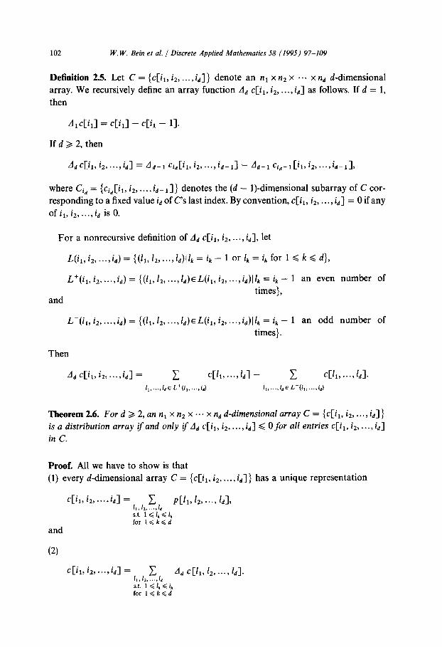
Definition 2.5. Let C = {c[i,, iz, . . . . id]} denote an nl x nz x ..* x nd d-dimensional array. We recursively define an array function Ad c[i,, iz, . . . . id] as follows. If d = 1,

then

AIc[iI] = c[iJ - c[i, - 11.

If d 2 2, then

Ad c[i,, iz, . ..) id] = Ad- 1 Cid[il, iz, . . . . id- J - Ad- 1 Ci,- 1 [ii, iz, . . ..id-ll.

where Ci, = {ci,[il, iz,...,id-r ]} denotes the (d - 1)-dimensional subarray of C cor-

responding to a fixed value id of c’s last index. By convention, c[i,, iz, . . . , id] = 0 if any of iI, il, . . . . id is 0.

For a nonrecursive definition of Ad c[iI, iz, . . . . id], let

L(iI, i2, . . . . id) = {(h, 12, . . . . ld)lh = ik - 1 or Ik = ik for 1 < k < d),

L+(&, iz , . ..) id) = {(iI, 12, . . . . kd)EL(il, izj . . . . id)1 lk = ik - 1 an even number of

and times),

L-(iI, iz, . . . . id) = {(l,, lz, . . . . ld)EL(il, iz, . . . . id)llk = ik - 1 an odd number of times}.

Then

Ad C[il, i2, . . ..id] = c c[l,, *..,ld] - c c&, .-.,ld].

1, ,..., IdEL+(iI ,..., id) I, ,.._, IdEL-(iI ,..., id)

Theorem2.6. Ford>,2,annIxn2x-.. x nd d-dimensional array C = {c[i,, i2, . . . . id]}

is a distribution array if and only if Ad c[iI, i2 , . . . . id] < ofor all entries c[il, i2, . . . . id]

in C.

Proof. All we have to show is that (1) every d-dimensional array C = {c[il, i2,. .., id] } has a unique representation

44, i2 >...yid] = I 1 ; I p[ll, 12, . . . . IdI, 1.2. *d

and

s.t. 1 4 Ik d i, for 1 $ k d d

(2)

c[il, i& . . ..id] = c 11,L...,ll

Ad ‘$11, 12, -.a, Id].

s.t. 1 $ I, Q ik for l<k<d

W. W. Bein et al. / Discrete Applied Mathematics 58 (1995) 97-109 103

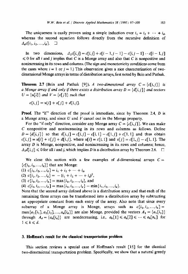
The uniqueness is easily proven using a simple induction over ii + iz + ... + i,,,

whereas the second equation follows directly from the recursive definition of Adc[iI, iz, . . . . id]. 0

In two dimensions, dzc[i,j] = c[i,j] + c[i - 1,j - l] - c[i,j - l] - c[i - l,j] < 0 for all i and j implies that C is a Monge array and also that C is nonpositive and

nonincreasing in its rows and columns. (The sign and monotonicity conditions come from the cases where i = 1 or j = 1.) This observation gives a nice characterization of two- dimensional Monge arrays in terms of distribution arrays, first noted by Bein and Pathak.

Theorem 2.7 (Bein and Pathak [9]). A two-dimensional array C = {c[i,j]} is

a Monge array if and only if there exists a distribution array D = {d[i, j] } and vectors

U = (u[i] > and V = (v[j] > such that

c[i, j] = u[i] + u[j] + d[i, j].

Proof. The “if” direction of the proof is immediate, since by Theorem 2.4, D is a Monge array, and since U and V cancel out in the Monge property.

For the “if only” direction, consider any Monge array C = (c[i, j] >. We can make C nonpositive and nonincreasing in its rows and columns as follows. Define D = {d[i,j]} so that d[i,j] = c[i,j] - c[i, l] - c[l,j] + ccl, l] and thus obtain c[i, j] = u[i] + v[j] + d[i, j], where u[i] = c[i, l] and v[j] = c[l,f - ccl, 11. The array D is Monge, nonpositive, and nonincreasing in its rows and columns; hence, Atd[i, j] < 0 for all i and j, which implies D is a distribution array by Theorem 2.6. cl

We close this section with a few examples of d-dimensional arrays C =

{cl%, iz, . . . . id]} that are Monge:

(I) cC&, iz, . . ., id] = iI + iz + a.. + id,

(2) cL 4, . . . . id] = - (iI + i2 + ... + id)‘,

(3) CL, i2 , . . . . id] = maxIi,, i2, . . . . id}, and (4) c[iI, i2, . . . . id] = max(il, i2, . . . . id} - min{ iI, i2, . . . . id). Note that the second array defined above is a distribution array and that each of the remaining three arrays can be transformed into a distribution array by subtracting an appropriate constant from each entry of the array. Also note that since every subarray of a Monge array is Monge, arrays such as c[i,, i2,. .., id] =

max(at Cd, a2Ci21, . . . . ad[id]} are also Monge, provided the vectors Ai = {aI[iI]}

through Ad = {a,,[iJ} are nondecreasing, i.e., ak[l] < ak[2] < ..a G ak[nJ for l<k<d.

3. Hoffman’s result for the classical transportation problem

This section reviews a special case of Hoffman’s result [15] for the classical two-dimensional transportation problem. Specifically, we show that a natural greedy

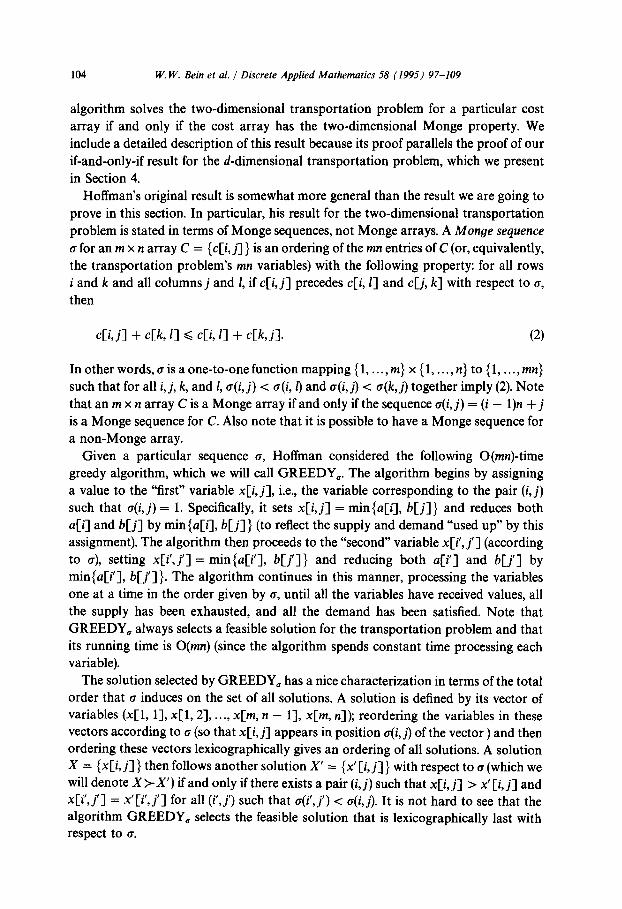
104 W. W. Bein et al. J Discrete Applied Mathematics 58 (1995) 97-109

algorithm solves the two-dimensional transportation problem for a particular cost array if and only if the cost array has the two-dimensional Monge property. We include a detailed description of this result because its proof parallels the proof of our if-and-only-if result for the d-dimensional transportation problem, which we present in Section 4.

Hoffman’s original result is somewhat more general than the result we are going to prove in this section. In particular, his result for the two-dimensional transportation problem is stated in terms of Monge sequences, not Monge arrays. A Monge sequence o for an m x n array C = {c[i, j] } is an ordering of the mn entries of C (or, equivalently, the transportation problem’s mn variables) with the following property: for all rows i and k and all columns j and 1, if c[i, j] precedes c[i, I] and c[j, k] with respect to 6, then

c[i, j] + c[k, 11 G c[i, 11 + c[k, j]. (2)

In other words, c is a one-to-one function mapping { 1, . . . , m} x { 1, . . . , n> to { 1, . . . , mn}

such that for all i, j, k, and I, a(i, j) < o(i, 1) and o(i, j) < a(k, j) together imply (2). Note that an m x n array C is a Monge array if and only if the sequence a(i, j) = (i - 1)n + j is a Monge sequence for C. Also note that it is possible to have a Monge sequence for

a non-Monge array. Given a particular sequence g, Hoffman considered the following O(mn)-time

greedy algorithm, which we will call GREEDY,. The algorithm begins by assigning a value to the “first” variable x[i, j], i.e., the variable corresponding to the pair (i, j) such that o(i, j) = 1. Specifically, it sets x[i, j] = min{a[i], b[j]} and reduces both a[i] and b[j] by min{a[i], 6[j]} (to reflect the supply and demand “used up” by this assignment). The algorithm then proceeds to the “second” variable x[i’, j’] (according to a), setting x[i’,j’] = min(a[i’], b[j’]} and reducing both a[?] and b[j’] by min{u[i’], b[j’]}. The algorithm continues in this manner, processing the variables one at a time in the order given by 0, until all the variables have received values, all the supply has been exhausted, and all the demand has been satisfied. Note that GREEDY,, always selects a feasible solution for the transportation problem and that its running time is O(mn) (since the algorithm spends constant time processing each variable).

The solution selected by GREEDY, has a nice characterization in terms of the total order that c induces on the set of all solutions. A solution is defined by its vector of variables (x[ 1, 11, x[ 1,2], . . ., x[m, n - 11, x[m, n]); reordering the variables in these vectors according to e (so that x[i, j] appears in position o(i, j) of the vector ) and then ordering these vectors lexicographically gives an ordering of all solutions. A solution X = {x[i, j]} then follows another solution X’ = {x’[i, j]} with respect to u (which we will denote X>X’) if and only if there exists a pair (i, j) such that x[i, j] > x’[i, j] and x[i’, j’] = x’[i’, j’] for all (i’, j’) such that o(i’, j’) < o(i, j). It is not hard to see that the algorithm GREEDY, selects the feasible solution that is lexicographically last with respect to 0.

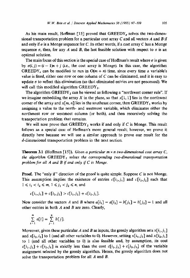
W.W. Bein et al. J Discrete Applied Mathematics 58 (1995) 97-109 105

As his main result, Hoffman [15] proved that GREEDY, solves the two-dimensional transportation problem for a particular cost array C and all vectors A and B if and only if 0 is a Monge sequence for C. In other words, if a cost array C has a Monge sequence o, then, for any A and B, the last feasible solution with respect to g is an optimal solution.

The main focus of this section is the special case of Hoffman’s result where Q is given by r+, j) = (i - 1)n + j (i.e., the cost array is Monge). In this case, the algorithm GREEDY, can be modified to run in O(m + n) time, since every time a variable’s value is fixed, either one row or one column of C can be eliminated, and it is easy to update d to reflect this elimination (so that eliminated entries are not processed). We will call this modified algorithm GREEDY2.

The algorithm GREEDY Z can be viewed as following a “northwest corner rule”. If we imagine embedding the array X in the plane, so that x[l, l] lies in the northwest corner of the array and x[m, n] lies in the southeast corner, then GREEDY2 works by assigning a value to the north- and westmost variable, which eliminates either the northmost row or westmost column (or both), and then recursively solving the transportation problem that remains.

We will now prove that GREEDY2 works if and only if C is Monge. This result follows as a special case of Hoffman’s more general result; however, we prove it directly here because we will use a similar approach to prove our result for the d-dimensional transportation problem in the next section.

Theorem 3.1 (Hoffman [15]). Given a particular m x n two-dimensional cost array C, the algorithm GREEDY2 solves the corresponding two-dimensional transportation problem for all A and B if and only if C is Monge.

Proof. The “only if” direction of the proof is quite simple. Suppose C is not Monge. This assumption implies the existence of entries c[il, jJ and c[iz, jzJ such that 1 < il < i2 < m, 1 < j, < j, d n, and

cC4,jJ + cCi2,j21 > cCi&l + cCb,jJ.

Now consider the vectors A and B where a[&] = a[&] = b[ j,] = b[ j,] = 1 and all other entries in both A and B are zero. Clearly,

iil @I = i Kd. j=l

Moreover, given these particular A and B as inputs, the greedy algorithm sets x[iI,j,] and x[iZ, i2] to 1 (and all other variables to 0). However, setting x[i1,j2] and x [i3, j,] to 1 (and all other variables to 0) is also feasible and, by assumption, its cost c[il, j,] + c[iz, j,] is strictly less than the cost c[il, j,] + c[iz,j,] of the variable assignment selected by the greedy algorithm. Hence, the greedy algorithm does not solve the transportation problem for all A and B.


For the “if” direction of the proof, suppose the lexicographically last feasible solution X is not optimal, and let X’ denote the lexicographically last solution that is optimal. By assumption, c(X) > c(X’) and X>X’. Now consider the lexicographically first variable x[i,f to which X and X’ assign different values. Since X follows X’ in the lexicographic ordering of solutions, we must have x[i, j] > x’[i, j]. Thus, in order to insure that the supply a[i] and the demand b[j] are both satisfied, X’ must assign nonzero values to at least two distinct variables x’[i, s] and x’[T, j] such that i < T < m and j < s < n. However, since C is Monge, we have

CM + 41, sl < c[i, s] + c[r, j].

Thus, reducing x’[i, s] and x’[r, j] by E = min{x’[i, s], x’[r, j]} and increasing x’[i, j] and x’[r, s] by this same E gives a new feasible solution X” such that c(X”) < c(X) and X”>X’. The existence of X” contradicts our assumption that X’ is the lexicographi- tally last optimal solution. 0

4. Our result for the d-dimensional transportation problem

In this section, we present our if-and-only-if result for the d-dimensional transportation problem.

We begin by defining our greedy algorithm. This algorithm, which we will call GREEDY,,, is the natural extension of the northwest-corner-rule greedy algorithm GREEDY2 described in the previous section. Our algorithm begins by setting x[l, 1, . ..) l] = min{al[l], az[l], . . . . a,,[l]}. We then reduce each of ui[l],

ml, **-, ad11 by min {adll, eC11, . . . . u,,[l]}. At least one of ui[l], uz[l], . . ..a.,[11 is thereby reduced to 0, which means we are done with the corresponding (d - l)- dimensional subarray of X. In other words, at least one of the problem’s dimensions

ni, n2,..., nd has been reduced by 1. The smaller transportation problem that remains can then be solved recursively.

The algorithm GREEDYd again selects the lexicographically last feasible solution, and its running time is 0(&r, + n, + 3.. + nd)), since each variable assignment takes O(d) time and reduces at least one of the problem’s dimensions by 1.

Theorem 4.1. Given a particular n, x n2 x “. x nd d-dimensional cost array C, the algorithm GREED Yd solves the corresponding d-dimensional transportation problem for

ull AI, A23 . . ., Ad ifund only if C is Monge.

Proof. The “only if” direction of the proof is again quite simple. Suppose C is not Monge. This assumption implies the existence of entries c[iI, i2, . . ., id] and

cCjhj2 , . . . , jd] such that


where Sk = min {ik, jk} and tk = max{ik, jk} for 1 < k < d. Note that the d-tuples (iI, i2, . . . . id), (jl,j2, . ..,j,), (sl, s2, . . . , sd), and (tr, t2,. . . , td) must be distinct. Now consider the vectors AI, AZ, . . . , Ad where for 1 < k < d, we have uk[ik] = 1 and a&,&] = 1 if ik # jk and &[ik] = 2 if ik = jk, and all other entries in Al, AZ, . . . , A,, are zero. Clearly,

i$l al[i] = f a2[i] = *.- = i=l

igl ud[il.

Moreover, given these particular Al, A2, . . . , Ad as inputs, the greedy algorithm sets

xcsr, s2, ***, sd] and x[t,, t2, . . . . td] to 1 (and all other variables to 0). However, the solution setting x[il, i2, . . . . id] and x[jr, j2 , . . ..j.] to 1 (and all other variables to 0) is also feasible, and, by assumption, its cost c[ir, i2, . . . , id] + c[ jr, j,, . . . ) jd] is strictly less than the COSt c[s1,s2,...,sd] -t c[tI,t2,..., td] of the solution selected by the greedy algorithm. Hence, the greedy algorithm does not solve the transportation problem for all Al, A2, . . . . A,,.

For the “if” direction of the proof, suppose the lexicographically last feasible solution X is not optimal, and let X’ denote the lexicographically last solution that is optimal. By assumption, c(X) > c(X’) and X>X’. Now consider the lexicographically first variable x[i,, it, . . . , id] to which X and X’ assign different values. Since X follows X’ in the lexicographic ordering of solutions, we must have x[i,, i2, . . . . id] > x’[il, i2, . . . . id]. Thus, in order to insure that the q[iJ, u2[i2], . . . . a&] are all satisfied, X’ must assign nonzero values to d variables

x’CjLjL . . ..$I

x’ Kk . . . , $1

x’Cjdl,jdz, . . ..A1

suchthatfor1~k~dand1~1~d,j~~i,,andfor1~k~d,j~=ik.Aildofthe d-tuples (j:, ji , . . . , ji) need not be distinct, but there must exist at least two of them, say

(jV,,jV,, . . . , j$ and (jy, j;, . . . . jr), neither of which dominates the other (i.e., there exist k and I such that j,U < j,W and jy > jr). However, since C is Monge, we have

CC%, s2, ..a, sd] + c[tl, t2 ? ..-,td] < c[j”,,ji , . . ..A1 + 4jYA . . ..jYl.

where sk = min{ j,V, jr} and tk = max{je, jr} for 1 < k < d. Furthermore, since neither of the d-tuples (jO,, jV,, . . . . ji) and (jy, jr, . . . . j,W) dominates the other, the d-tuples

(% s 2, . . ..sd) and 01, t2, ***, td) must be distinct from (jV,, j”,, . . . . j$ and (jy, jy, . . . . jr). Thus, reducing x’[jy, jV,, . . . . ji] and x’Ey, j;, . . . . j,W] by

E = min(x’[jy,jp ,..., ji], x’[jy,jy, . . . . jr])

and inCreaSing x'[s~,s~,...,~~] and X'[t,, TV,..., td] by this same E gives a new feasible

solution X” such that c(X”) < c(X’) and X”>X’. The existence of X” contradicts our assumption that X’ is the lexicographically last optimal solution. 0


5. Concluding remarks

We conclude with two remarks: (1) Closely related to the d-dimensional transportation problem is the d-dimen-

sional assignment (or matching) problem. The assignment problem is a transportation problem where (a) all the dimensions have equal size (i.e., uk = n for 1 < k < d),

(b) all the supply-demands are 1 (i.e., &[ik] = 1 for 1 < k < d and 1 < ik < n), and (c) the variables x[ii, il, . . . , id] are restricted to be integers.

For d 2 3, the general d-dimensional assignment problem is NP-hard (see [14], for example). However, if the assignment problem’s cost array is Monge, then the solution given by

x[ii, iz, . . ..&I = i

1 if i1 = iZ = . . . = id,

0 otherwise

must be optimal, as our greedy algorithm will always produce this solution. (2) In this paper, we have focused on generalizing the Monge-array formulation of

Hoffman’s work. A natural question to ask is whether Hoffman’s notion of a Monge sequence also generalizes to higher dimensions. We believe that it does, though the property defining a d-dimensional Monge sequence seems to be a bit more complic- ated than the property defining a d-dimensional Monge array. (Specifically, the Monge-sequence property relates 2d entries of the cost array, while the Monge-array property relates only 4 entries.) However, we have not pursued this line of investiga- tion, as the natural Monge-sequence greedy algorithm takes O(n”) time to solve an n x n x a-. x n d-dimensional transportation problem, making the Monge-sequence case of somewhat less interest than the Monge-array case, where the greedy algorithm runs in 0(d2n) time.

References

[l] A. Aggarwal, M.M. Klawe, S. Moran, P.W. Shor and R. Wilber, Geometric applications of a matrix-

121

c31

M

PI

searching algorithm, Algorithmica 2 (1987) 195208. ._

A. Aggarwal and J.K. Park, Parallel searching in multidimensional monotone arrays, Research Report RC 14826, IBM T.J. Watson Research Center, Yorktown Heights, NY (1989); Submitted to J. Algorithms; Portions of this paper appear in Proceedings of the 29th Annual IEEE Symposium on Foundations of Computer Science (1988) 497-512. A. Aggarwal and J.K. Park, Sequential searching in multidimensional monotone arrays, Research Report RC 15128, IBM T.J. Watson Research Center, Yorktown Heights, NY (1989); Submitted to J. Algorithms; Portions of this paper appear in Proceedings of the 29th Annual IEEE Symposium on Foundations of Computer Science (1988) 497-512. A. Aggarwal and J.K. Park, Improved algorithms for economic lot-size problems, Oper. Res., to appear; An earlier version of this paper appears as Research Report RC 15626, IBM T.J. Watson Research Center, Yorktown Heights, NY (1990). M.J. Atallah, S.R. Kosaraju, L.L. Larmore, G. Miller and S. Teng, Constructing trees in parallel, in: Proceedings of the 1st Annual ACM Symposium on Parallel Algorithms and Architectures (1989) 421431.


[6] W.W. Bein, Netflows, polymatroids, and greedy structures, PhD thesis, Universitat Osnabrtick, Osnabriick (1986).

[7] W.W. Bein, P. Brucker and A.J. Hoffman, Series parallel composition of greedy linear programming problems, Research Report RC 17834, IBM T.J. Watson Research Center, Yorktown Heights, NY (1992); Submitted to Math. Programming.

[8] W.W. Bein, P. Brucker and P.K. Pathak, Monge properties in higher dimensions, Technical Report CS90-11, Department of Computer Science, University of New Mexico, Albuquerque, NM (1990).

[9] W.W. Bein and P.K. Pathak, A characterization of the Monge property, Technical Report CS90-10, Department of Computer Science, University of New Mexico, Albuquerque, NM (1990).

[lo] R.E. Burkard, Assignment problems: Recent solution methods and applications. in: A. Prekopa, J. Szelezsan and B. Straxicky, eds., System Modelling and Optimization: Proceedings of 12th IFIP Conference, Budapest, Hungary, September 26, 1985, Lecture Notes in Control and Information Sciences 84 (Springer, New York, 1986) 153-169.

[11] K. Cechlarova and P. Sxabo, On the Monge property of matrices, Discrete Math. 81(1990) 123-128. [12] D. Eppstein, Z. Gal& R. Giancarlo and G.F. Italiano, Sparse dynamic programming, in: Proceedings

of the 1st Annual ACM-SIAM Symposium on Discrete Algorithms (1990) 513-522. [13] M. Fahimi and P.K. Pathak, Applications of a size reduction technique for transportation problems

in sampling, in: Proceedings of the First International Symposium on Optimization and Statistics, Aligarh, India (1989).

[14] M.R. Garey and D.S. Johnson, Computers and Intractability: A Guide to the Theory of NP- Completeness (Freeman, San Francisco, CA, 1979).

[ 151 A.J. Hoffman, On simple linear programming problems, in: V. Klee, ed., Convexity: Proceedings of the Seventh Symposium in Pure Mathematics of the AMS, Proceedings of Symposia in Pure Mathemat- ics 7 (American Mathematical Society, Providence, RI, 1963) 317-327.

[16] L.L. Larmore and T.M. Przytycka, Parallel construction of trees with optimal weighted path length, in: Proceedings of the 3rd Annual ACM Symposium on Parallel Algorithms and Architectures (1991) 71-80.

[17] L.L. Larmore and B. Schieber, On-line dynamic programming with applications to the prediction of RNA secondary structure, J. Algorithms 12 (1991) 49&515.

[18] G. Monge, Mtmoire sur la thtorie des deblais et des remblais, in: Histoire de l’Acadbmie Royale des Sciences, Annee M. DCCLXXXI, avec les Memoires de Mathematique et de Physique, pour la m&me An&e, Tires des Registres de cette Academic (L’Imprimerie Royale, Paris, 1784) 666704.

[19] J.B. Orlin, A faster strongly polynomial minimum cost flow algorithm, Oper. Res., to appear; An earlier version of this paper appears in Proceedings of the 20th Annual ACM Symposium on Theory of Computing (1988) 377-387.

[ZO] H.M. Wagner, On a class ofcapacitated transportation problems, Management Sci. 5 (1959) 304318. [21] F.F. Yao, Efficient dynamic programming using quadrangle inequalities, in: Proceedings of the 12th

Annual ACM Symposium on Theory of Computing (1980) 429-435.

Documents

A Monge property for the d-dimensional transportation problem · A Monge property for the d-dimensional transportation ... the French mathematician Gaspard Monge, ... The d-dimensional