A Monte Carlo model for estimating tornado impacts

METEOROLOGICAL APPLICATIONSMeteorol. Appl. (2016)Published online in Wiley Online Library(wileyonlinelibrary.com) DOI: 10.1002/met.1552

A Monte Carlo model for estimating tornado impacts

Stephen M. Strader,* Thomas J. Pingel and Walker S. AshleyMeteorology Program, Department of Geography, Northern Illinois University, DeKalb, IL, USA

ABSTRACT: Determining the likelihood and severity of tornado disasters requires an understanding of the dynamicrelationship between tornado risk and vulnerability. As population increases in the future, it is likely that tornado disasterfrequency and magnitude will amplify. This study presents the Tornado Impact Monte Carlo (TorMC) model, which simulatestornado events atop a user-defined spatial domain to estimate the possible impact on people, the built-environment or otherpotentially vulnerable assets. Using a Monte Carlo approach, the model employs a variety of sampling techniques on observedtornado data to provide greater insight into the tornado disaster potential for a location. Simulations based on 10 000 years ofsignificant tornado events for the relatively high-risk states of Alabama, Illinois and Oklahoma are conducted to demonstratethe model processes, and its reliability and applicability. These simulations are combined with a fine-scale (100 m), residentialbuilt-environment cost surface to illustrate the probability of housing unit impact thresholds for a contemporary year. Sampleresults demonstrate the ability of the model to depict successfully tornado risk, residential built-environment exposure andthe probability of disaster. Additional outcomes emphasize the importance of developing versatile tools that capture betterthe tornado risk and vulnerability attributes in order to provide precise estimates of disaster potential. Such tools can provideemergency managers, planners, insurers and decision makers a means to advance mitigation, resilience and sustainabilitystrategies.

KEY WORDS tornado; Monte Carlo; impacts; exposure; risk; disaster

Received 11 September 2015; Revised 3 December 2015; Accepted 11 December 2015

1. Introduction

Over the last 80 years, the frequency and magnitude ofweather-related disasters and losses have been increasing(Bouwer, 2011; Smith and Katz, 2013). The attributionof the underlying cause for the observed amplification inweather-related disaster frequency and magnitude is a con-tentious topic (Pielke, 2005; Bouwer, 2011; Huggel et al., 2013;Kunkel et al., 2013). However, at the most fundamental levelit involves the juxtaposition of a hazard event (e.g. risk of atornado) with people and their assets (e.g. vulnerability of acertain segment of the populace, housing, critical infrastructure,to a tornado) that determines disaster potential, consequence andseverity. To date, there has been limited research determininghow risk and vulnerability interact to shape tornado disastercharacteristics. Even less attention has been paid to developingtools and methodologies to examine the dynamic relationshipbetween tornado risk and vulnerability.

In the present research, tornado risk is defined as the spatiotem-poral probability of tornado occurrence, or hazard, of a certainmagnitude, whereas tornado vulnerability is represented by abasic physical exposure metric (e.g. the number of individuals,households or some other tangible asset potentially affected by atornado). While vulnerability includes other components – suchas adaptive capacity (i.e. coping, or adapting, to a hazard) andsensitivity (i.e. degree to which a system is impacted by a haz-ard), these components and their interactions are often very

* Correspondence: S. M. Strader, Meteorology Program, Department ofGeography, Northern Illinois University, Davis Hall, Rm. 118, DeKalb,IL 60115, USA. E-mail: [email protected]

complex and difficult to quantify at a high resolution across alarge spatiotemporal domain (Cutter et al., 2009; Morss et al.,2011). For this reason, this study focuses on a quantifiable andwell-measured variable, the housing unit (HU), to exemplifyaspects and utility of the model.

The initial goal of this research is to present a tool that exam-ines the interaction of tornado risk and vulnerability to mea-sure tornado disaster frequency, magnitude and disaster poten-tial better, whether from a historical or future perspective. Thedescribed Tornado Impact Monte Carlo (TorMC) model simu-lates years of tornado events atop a geographical region whileassessing their impacts, or costs, on the underlying physical vul-nerability landscape. To demonstrate the utility and efficacy ofthe TorMC model, 10 000 years of significant (≥Enhanced FujitaScale 2 magnitude or EF2+) tornadoes were simulated for thestates of Alabama, Illinois and Oklahoma to estimate the num-ber of HUs affected by each path in an hypothetical contemporaryyear. Simulation results as well as model sensitivity and reliabil-ity are highlighted through a number of statistical and graphicalprocedures.

2. Background

As populations continue to grow, the increased placement of peo-ple and their assets in physically vulnerable locations is leadingto greater disaster potential (Changnon et al., 2000; Nicholls andSmall, 2002; Burkett and Davidson, 2012; Ashley et al., 2014;Ashley and Strader, 2015; Strader and Ashley, 2015). Recentstudies have sought to examine tornado risk and vulnerability(namely, the exposure component) by using geographic infor-mation systems (GIS). Over the last decade, advancements inGIS capabilities and affiliated datasets have permitted studies to

© 2016 Royal Meteorological Society

S.M. Strader et al.

superimpose tornado events or their likeness atop exposure land-scapes to analyse potential tornado impacts and losses on popu-lations (Rae and Stefkovich, 2000; Wurman et al., 2007; Ashleyet al., 2014; Rosencrants and Ashley, 2015). Recent research hasalso coupled Monte Carlo (MC) simulation methods with thetornado hazard to provide greater insight into tornado incidence(Meyer et al., 2002) and impacts on policyholders (Daneshvaranand Morden, 2007). MC simulation is a computational modellingtechnique that employs repeated random sampling to obtain thedistribution of an unknown probabilistic entity (Mooney, 1997).This technique is distinguished from other types of computa-tional models because of two unique characteristics, iteration andrandomness. The ability of MC simulations to provide proba-bilistic rather than deterministic solutions yields greater value tostakeholders and those with a vested interest as it provides moreinformation about likely ‘best case’ and ‘worst case’ outcomes.

In the last 2 decades, MC simulations were employed in thefield of hazard sciences to examine the effects and consequencesof relatively rare, yet high-impact, geophysical events (Meyeret al., 2002; Rahman et al., 2002; Apel et al., 2004; Daneshvaranand Morden, 2007). In the hazards research community, MC sim-ulations have often been employed to acquire probability distri-butions (Meyer et al., 2002), return intervals or periods (Rahmanet al., 2002; Daneshvaran and Morden, 2007) and/or probabilityof exceedence (POE) measures of extreme events (Apel et al.,2004). More recently, models employing MC simulation tech-niques were developed in the reinsurance and catastrophe mod-elling fields (e.g. Aon Impact Forecasting, Swiss Re, Gen Re).However, most of these models are proprietary and unavailableto researchers. To date, only two available studies (Meyer et al.,2002; Daneshvaran and Morden, 2007) have applied MC simu-lation techniques to the tornado hazard. The MC simulation ina study by Meyer et al. (2002) used random sampling from sta-tistical distributions of tornado characteristics (i.e. occurrence,number of tornadoes, path length and width, magnitude) to modelsolely significant tornado occurrence in the conterminous UnitedStates. In the study by Daneshvaran and Morden (2007), the AonImpact Forecasting Monte Carlo model is highlighted. They usedMC methods to simulate tornado occurrence probabilities andreturn periods as well as potential losses for their policyholdersin the United States.

3. TorMC model design

There are ∼65 years of functional tornado data, with muchof the data subject to inaccuracy and bias (e.g. Brooks et al.,2003; Doswell, 2007). Even when controlling for these dataissues and non-meteorological biases, small sample size remainsa paramount issue for research studying the climatology ofthese relatively rare events (Doswell, 2007). MC simulationspaired with tornado hazards (i.e. the TorMC model) do notpresent more accurate or realistic measures of tornado risk andclimatology because their inputs remain bounded by the envelopeof observed events; rather, they provide a larger ‘snapshot’ or‘window’ of tornado event outcomes based on historical data.It is entirely plausible that, given the small sample size ofobserved tornado data, extremes, or ‘tails’ of the distribution,event attribute values (e.g. length, width, magnitude, count) havenot been captured adequately over the last 65 years. Tornadoevents and their characteristics could be occurring potentiallyin patterns for thousands of years or more (Meyer et al., 2002;Doswell, 2007). In addition, previous research examining thedisaster consequences for a location have been constrained by

the number of tornado paths employed and the tornado pathplacement. The major advantage of the TorMC model is that itpermits the estimation of regional disaster probability throughtens of thousands of simulated tornado events in contrast to only ahandful of outcomes. Thus, the TorMC model provides an overallbetter grasp of large-scale tornado risk and potential tornadoimpact variability.

The TorMC model comprises four general steps: (1) studyregion and model parameter definition; (2) tornado footprint cre-ation; (3) tornado cost assessment, and (4) output production(Figure 1). The TorMC model was designed to be highly modular(Petersen, 2012) in order to provide a user with as many simu-lation options as possible. Model parameter choices are selectedprior to executing the program and allow the user to control thetype of output generated by the TorMC model. Model parame-ters, steps, considerations and caveats are discussed hereafter.

3.1. Study region

The first step of the model process begins with the users defininga study domain on which they want to perform the MC sim-ulation. The TorMC model is compatible with a study area ofany shape or size (e.g. conterminous United States, state, countyor custom) in shapefile (.shp) format. As illustrated by previ-ous studies employing tornado MC methods (Meyer et al., 2002;Daneshvaran and Morden, 2007), the study area size should be80 km2 or greater. This area corresponds to the Storm PredictionCenter’s (SPC) probability forecasts that signify the chance ofsevere weather within 40 km of any point in the United States(Brooks et al., 2003). Domains smaller than 80 km2 may resultin an underestimation of tornado occurrence within the regiondue to the limited observed tornado record and small samplesize (∼59 000 events in the conterminous United States (Doswell,2007)).

Edge effects occur in models that sample lines with startingpoints, preferred azimuths and ending points that fall outsidea domain (e.g. TorMC model simulated tornado paths). As themajority of tornadoes in the United States move from southwestto northeast (Suckling and Ashley, 2006), an under-sampling oftornadoes is apparent in a user-selected region’s south and westsides (Figure 2). This edge effect is removed or corrected forin the TorMC model by adding a simple 100 km buffer to thestudy area and thereafter sampling all events within the buffer. Aclipping routine, which is discussed in a forthcoming section, islater used in the model to reclaim the user’s original domain.

3.2. Tornado counts

The TorMC model attempts to simulate tornado eventsby using historical data acquired from the SPC SVRGIS(http://www.spc.noaa.gov/gis/svrgis/) data. Although there aremany issues with the observed tornado data (e.g. width (Brooks,2004; Strader et al., 2015a); reporting bias (Brooks et al., 2003;Doswell et al., 2005; Anderson et al., 2007); counts (Brookset al., 2003; Verbout et al., 2006; Tippett et al., 2015)), thesedata are the only accessible source of extensive tornado eventinformation. The SVRGIS tornado shapefile, which contains theobserved tornado record, is integrated into the TorMC model.This permits the sampling of historical event lengths, widths,years, starting locations, ending locations and magnitudes.

The number of simulated tornadoes is based on the observedSVRGIS tornado data within the user-provided study region byrandomly selecting an annual tornado count from a given yearin the historical data (1950–2014) using a bootstrap (Efron and

© 2016 Royal Meteorological Society Meteorol. Appl. (2016)


Figure 1. Tornado Impact Monte Carlo (TorMC) model flow chart. Rhombus shapes indicate model input parameters, squares represent modelprocesses, rounded-corner rectangles denote simulation decisions or choices and the oval highlights the model output or ending process.

Tibshirani, 1994), or random sampling with replacement, tech-nique. Although the SVRGIS data contain information as farback as 1950, annual tornado counts from 1950 to 1953 areoften removed because they are considerably less complete andare of a lower quality than those from 1954 to 2014 (Agee andChilds, 2014). These abnormal counts are attributed to differentsources of tornado event information (i.e. U.S. Nuclear Regula-tory Commission; Grazulis, 1993) prior to the establishment ofthe National Severe Storms Forecast Center in 1952. Althoughit is preferable to remove 1950–1953 from the considered data,the user does have the capability to randomly sample randomlythe annual tornado counts (adjusted or unadjusted) and theirattributes from any available SVRGIS temporal range as well asother sources of data (e.g. Grazulis, 1993) that fit the SVRGISformat.

The TorMC model does not determine an exact number oftornadoes to produce; rather, it simulates years of tornado events.For instance, the model user may want to generate 10 000 years oftornado events atop a particular study region. The TorMC modelwould then randomly sample or select an annual tornado countfrom a single SVRGIS data year (1954–2014) within the studyregion. This randomly chosen count would then represent thetotal number of tornadoes the model will generate during the firstyear of simulation. In this case, the process would be repeated

9999 more times, with replacement, until each simulation yearcontains a total number of tornadoes to create. The benefit ofsimulating tornadoes during a given year is to capture better theinherent year-to-year variability in annual tornado occurrencesacross a study region.

3.3. Tornado magnitudes

Next, the user must also decide what magnitude of tornadoes tosimulate. The user can choose to generate a single magnitude(i.e. EF0, EF1 etc.) tornado class or a range of tornado magni-tudes (e.g. (EF0+), significant (EF2+) and violent (EF4+)). TheTorMC model acknowledges but makes no attempt to correctfor the known bias towards higher tornado intensity ratings priorto 1970 (Verbout et al., 2006; Thorne and Vose, 2010; Edwardset al., 2013). Future TorMC versions will accommodate andrectify any known tornado magnitude or intensity rating biases.Nevertheless, tornado occurrences are progressively rarer asmagnitude increases; the TorMC model accounts for this varia-tion by modifying the total number of tornadoes to construct in aparticular simulation year. For instance, if the user wants to gen-erate 10 000 years of violent tornadoes across the studied region,only those observed tornado events that are within the studyregion and meet the user-defined magnitude criteria (EF4+)


S.M. Strader et al.

Figure 2. Point density map representing tornado ending points (longitude, latitude) from a 10 000 year Tornado Impact Monte Carlo (TorMC)simulation for the state of Alabama. (a) Illustrates the non-corrected edge effects, while (b) highlights the corrected edge effects from the buffer-clip

(inflation–deflation) procedure.

will be considered in the randomly sampled SVRGIS year. Thisprocess ensures that there will not be under- or over-samplingof tornadoes at a given magnitude, while an approximate rep-resentation (based on observed record) of tornado counts bymagnitude will be created for all TorMC model simulation years.

Once the TorMC model selects a random SVRGIS year andits associated observed tornado count, it then develops a sec-ond bootstrap sample to select a particular magnitude of tor-nado to simulate. This sampling process is then repeated untilthe desired total number of simulation years is reached. Boot-strap re-sampling captures the potential variability in tornadomagnitudes in a year while also taking the relative percentageof all events of a given magnitude into account. For example,if a user chooses to generate significant tornado paths atop thestudy region from 1954 to 2014, the model will randomly selecta year’s significant annual tornado path count as the total numberof paths to generate in the first simulation year. In this randomlychosen year, there may be 50 (30 EF2, 15 EF3, 4 EF4 and 1 EF5)significant tornadoes within the study region. The model wouldthen randomly select one tornado magnitude, record it, place itback into the empirical data and repeat the process 49 more timesuntil it captures a list of 50 tornado magnitudes for that simula-tion year. In this case, the user can expect the model to generatemore EF2 than EF5 magnitude events simply based on their prob-ability of occurrence.

3.4. Tornado lengths and azimuths

Initially, the azimuths of all tornado paths within the regionallyfiltered SVRGIS data are calculated. An azimuth is then chosenrandomly from the data based on the previously selected tornadomagnitude within the study region. Because tornado azimuthsare not random and have a climatological tendency to travel inparticular directions in the conterminous United States (Sucklingand Ashley, 2006), this process captures the character of tornadopath azimuths within the study region. The procedure ensures

that a simulated tornado of a given magnitude would have itsazimuth correspond to that of an observed tornado with thesame magnitude in the study region. The tornado path lengthis also selected using this method by pairing simulated tornadolengths with observed tornado lengths within the same magnitudeclass. The model can also employ random sampling from modeldistributions (e.g. Weibull) and their fits from the observed dataas opposed to sampling directly from the historical observed data.

3.5. Tornado widths

Similar to Meyer et al. (2002) and Brooks (2004), simulated tor-nado path widths are determined by bootstrap sampling from aWeibull distribution fit on the observed tornado width data bytornado damage rating or magnitude in the study region. TheWeibull distribution was chosen because it is non-negative andalways positively skewed (Brooks, 2004). The primary advan-tage of using a statistical distribution (as opposed to bootstraptechniques) to model tornado path widths is that the Weibull dis-tribution characterizes actual tornado widths better by EF scalemagnitude compared with observed widths while at the sametime reducing the effects of abrupt and apparent step functions inthe historical tornado width data caused by systematic changes inevent-recording practices. For instance, 1950–1994 tornado pathwidths were denoted by the mean path width and transitioned toreported maximum path widths by 1995 (Brooks, 2004; Ageeand Childs, 2014; Strader et al., 2015a). A second modificationin tornado reporting practices occurred in 2007 with the imple-mentation of the EF scale. Although unrelated to tornado pathwidth reporting practices, this change to the EF scale in 2007 hasproduced, as a whole, wider tornado path widths. The reasonsfor this increase in tornado widths post EF-scale implementationare not known. To apply this modelling option, the TorMC modelrequires the user to provide a comma-separated values parameterfile containing the alpha (shape) and beta (scale) parameters bytornado magnitude that the model calls upon to generate random



Figure 3. Shows 10 000 randomly generated longitude and latitude points on the surface of the earth. (a) Indicates the clustering of points near thepoles, which results from simple uniform random generation, while (b) illustrates the spatially correct random points.

tornado widths. The model also accommodates the simulation oftornado path widths using random sampling with replacement ifthe user prefers this technique.

3.6. Tornado placement

The first tornado initiation option randomly generates latitudeand longitude co-ordinates within the study region that serveas the touchdown locations for each simulated tornado. If ran-dom points are being generated on a spherical surface they willhave a tendency to cluster near the poles due to converging(non-parallel) lines of longitude (Weisstein, 2002a; Figure 3).However, the TorMC model corrects for any spatial bias that mayarise during this step by employing an algorithm that randomlycreates latitude and longitude co-ordinates within the study area(Weisstein, 2002a). An equal tornado touchdown likelihood inthe study region may be sufficient for relatively small geograph-ical areas (e.g. regional) but potentially problematic on largerscales (e.g. conterminous United States) due to climatologicaldifferences in tornado occurrences within the United States (e.g.Dixon et al., 2011; Farney and Dixon, 2014; Tippett et al., 2015).Given this issue, the second tornado start location creation optionconsiders the potential variation in tornado touchdown probabil-ity in a study region. This method requires the user to provide atornado touchdown probability raster surface (e.g. cf. figure 4 inBrooks et al., 2003) on which the start locations will be spatiallyweighted. The second methodology is suitable at all geographi-cal spatial scales and provides a greater advantage in increasinglylarger, user-defined study regions. The tornado event simulationportion of the TorMC model concludes with the creation of tor-nado footprint polygons (i.e. maximum areal extent of tornadicwinds or tornado length multiplied by width) with the spatialextent and orientation controlled by the simulated path lengths,widths and azimuths.

3.7. Cost extraction

The cost extraction portion of the model begins with the secondstep in the edge correction process by clipping spatially the

tornado polygons using the original, user-defined study region.The next step employs the user-provided raster cost surfaceto assess the tornado impact. Prior to running the model, theuser must provide the raster cost surface on which the TorMCmodel will calculate zonal statistics (i.e. the summarization ofgeospatial raster datasets based on vector geometries) using thegenerated tornado footprint polygons. The model accommodatesany type of raster cost surface (continuous or categorical) aslong as the user defines a cost field within the raster. The zonalstatistics portion of the model permits a variety of statisticalcalculation options (e.g. mean, sum). If the user provides araster cost surface of gridded population, a sum statistic optioncomputes a zonal statistic representing the total number of peopleaffected by each tornado path.

The user has the option to apply different types ofcost-extraction techniques – e.g. ‘centroid within’ and ‘inter-sect’ (Figure 4). These methods affect the zonal statisticscalculation for each tornado footprint. The centroid withinextraction method calculates zonal statistics solely for thoseraster cells where the tornado footprint intersects the centroidof the cell, while the intersect extraction technique includes allthe raster cells that are touched by a tornado footprint in thezonal statistics calculation. Although not a part of this TorMCiteration, the ‘completely within’ and ‘areal weight’ techniquesprovide additional means of cost extraction. The completelywithin method includes all raster cells that are contained withinthe bounds of the tornado footprint. The areal weight (AW)method (Schlossberg, 2003; Balk et al., 2005; SEDAC, 2015;Ashley et al., 2014) provides a more accurate measure of tor-nado costs, especially for those grid cells along the edges of thetornado footprint. Where a tornado footprint transects portionsof grid cells, cost tallies (e.g. HUs) are adjusted based on theareal fraction of the grid cells affected (Figure 4). For example, ifa tornado path bisects a grid cell representing 100 HUs, then thetotal number of HUs impacted by the tornado in that grid cell is50 (i.e. 0.50 × 100 HU = 50 HUs). This process is then repeatedfor all grid cells that the tornado footprint traverses. Eachcost-extraction technique is heavily influenced by the spatial


S.M. Strader et al.

Figure 4. Illustration of centroid within, intersect, completely within and areal weighted (AW) cost-extraction techniques. The grid cells representthe cost surface with black dots comprising the centroid of each cell, and the non-shaded rectangle signifies a potential tornado footprint. Shadedgrid cells indicate those that would be included in the tornado cost calculation during each type of cost-extraction method (after Schlossberg, 2003).

resolution, or cell size, of the raster cost surface. For instance, araster surface with low spatial resolution in combination with thecentroid method would result in an underestimation of tornadocosts. In general, a raster with a high spatial resolution will leadto superior estimates of impact.

3.8. Model output

The TorMC model yields both .shp and .csv files representingthe TorMC geo-dataframe with various simulation data fields.Fields generated include unique tornado field identifier (FID),projected footprint polygon geometry, starting latitude andlongitude, ending latitude and longitude, path length (km) andwidth (km), azimuth (∘), magnitude (0–5), simulation year andzonal statistics.

4. TorMC model application

4.1. Model performance

To illustrate the model’s reliability and performance, a simula-tion based on 10 000 years of significant tornadoes across thestate of Oklahoma was conducted initially. Significant tornadoeswere simulated as they have been responsible for 98.8% of alltornado fatalities and a majority of tornado damage since 1950(Ashley, 2007; Simmons and Sutter, 2007). In addition, signifi-cant tornado event frequency has remained consistent since 1950,while non-significant tornado event frequency has risen substan-tially due to non-meteorological influences (e.g. Doswell, 2007).

Oklahoma is a suitable candidate for examining model perfor-mance due to its elevated significant tornado risk and relativelylarge population centres exposed to this risk (e.g. Oklahoma Cityand Tulsa). After testing a variety of simulation lengths, 10 000years was a period of record that produced functional, yet com-putationally efficient, output. The 10 000 year significant tornadosimulation was coupled with a gridded, fine-scale (100 m) resi-dential built-environment cost surface, representing HUs acrossOklahoma in the year 2010. The HU cost surface is derivedfrom the Spatially Explicit Regional Growth Model (SERGoM;Theobald, 2005), which employs a variety of geospatial data suchas water bodies, protected areas, Census block population, roaddensity, etc., to determine HU density at the 100 m scale in theconterminous United States. SERGoM data accuracy and relia-bility were measured using a hindcast technique, with the modeloutput comparable to Census data (Theobald, 2005).

Tornado counts from 1954 to 2014 were considered, whiletornado widths were modelled using the Weibull parameters out-lined by Brooks (2004). Tornado lengths, azimuths and magni-tudes were selected using a bootstrap sampling technique on theobserved tornado data. For the present study, a random tornadotouchdown probability coupled with the intersect cost-extractionmethod was used although it may remove any potential climato-logical patterns of tornado occurrence and attributes. However, apotential benefit in using this tornado placement technique is thatit avoids tornado reporting bias that may be, in part, due to pop-ulation density (e.g. Doswell et al., 2005). This bias is evidentwhen comparing observed significant tornadoes (Figure 5(a))to the randomly chosen 61 simulation years (Figure 5(b)). In



Figure 5. (a) Observed SVRGIS significant (EF2+) tornado footprints from 1954 to 2014 (dark black lines) with the SERGoM total number ofhousing units (HU) per ha in 2010 for the state of Oklahoma. (b) Same as in panel (a) but with a random 61 years of simulated significant tornadofootprints. (c) Same as in panel (a) except for the TorMC’s 10 highest annual HU impact years. The period of 61 years was selected because that was

the temporal range of observed historical events used in the Tornado Impact Monte Carlo (TorMC) simulations.

this case, clustering of significant tornado footprints around theOklahoma City metropolitan area is apparent in the observedhistorical tornado data, while the TorMC-simulated footprintplacement illustrates a random pattern.

Over the 10 000 year simulation, the TorMC model gener-ated 116 045 significant tornadoes, with 73.8% EF2, 20.6% EF3,5.1% EF4 and 0.6% EF5 tornadoes (Table 1). The simulated per-centages of tornadoes by EF magnitude are similar to those from

Oklahoma’s observed record from 1954 to 2014 (i.e. 71.6% EF2,21.2% EF3, 6.3% EF4 and 0.9% EF5). The model produced amean (median) of 11.6 (10) significant tornadoes per year overthe 10 000 year simulation with a violent tornado occurring every1.5 years (Table 2). This represents a 66% chance a violent tor-nado will traverse Oklahoma in a given simulation year. A ran-dom sample of 61 years was chosen from the 10 000 year sim-ulation (sample period) and compared to the observed tornado


S.M. Strader et al.

Table 1. Significant and violent tornado attributes from the 10 000 year TorMC model simulation for the state of Oklahoma. Tornado EF magnitude,count, mean annual count, mean length, mean width, mean azimuth are denoted.

Magnitude Count Mean annual count Mean length (km) Mean width (m) Mean azimuth (∘)

EF2 85 645 8.56 12.01 122.44 66.89EF3 23 846 2.38 25.64 262.45 66.08EF4 5919 0.59 51.19 457.40 67.21EF5 635 0.06 63.87 551.45 67.58EF2+ (Significant) 116 045 11.60 17.09 170.64 66.74EF4+ (Violent) 6554 0.66 52.42 466.51 67.25

Table 2. TorMC model results from a 10 000 year simulation of significant tornadoes atop the state of Oklahoma. Tornado event EF magnitude,return period, annual occurrence probability, the mean number of HUs affected by a given tornado and the mean number of HUs impacted by all

tornadoes in a simulation year are indicated.

Magnitudea Return period (years) Annual occurrence probability Mean tornado impact (HU) Mean annual impact (HU)

EF2 0.12 8.56 24.53 210.07EF3 0.42 2.38 73.62 175.56EF4 1.69 0.59 205.84 121.84EF5 15.75 0.06 306.76 19.48EF2+ (Significant) 0.09 11.60 45.41 526.94EF4+ (Violent) 1.53 0.66 215.62 141.32

aGiven the distribution of tornadic winds within a footprint, only a small percentage of the total HUs affected by the tornado footprints are subject to significant or violenttornado wind speeds (e.g. Strader et al., 2015a).

data of 1954–2014 (observed period). Comparisons between thesample and observed record revealed a consistent median numberof significant tornadoes per year (11), while the mean number ofsignificant events per year was 14.6 and 12.1 for the observed andsample periods, respectively. The statistical difference betweenthe randomly sampled 61 simulated years and observed years isattributed to the year-to-year variability of simulated significanttornado counts. The percentages of tornadoes by EF magnitudefor the observed (71.6% EF2; 21.2% EF3; 6.3% EF4; 0.9% EF5)and sampled (73.2% EF2; 21.0% EF3; 4.3% EF4; 1.5% EF5)periods are also similar, revealing that the TorMC model datamirrors the observed data.

The 10 000 year Oklahoma simulation generated mean signif-icant tornado length and width of 17.1 km and 170.6 m, respec-tively (Table 1). Compared to the observed data, and as illustratedin Brooks (2004) and Strader et al. (2015a), tornado length andwidth typically increase as EF magnitude escalates. Mean tor-nado lengths for significant tornadoes ranged from 12 km (EF2)to 63.9 km (EF5), while mean tornado widths varied from 122.4m (EF2) to 551.5 m (EF5). All mean simulated tornado lengthsby EF magnitude are within 5 km of the corresponding empiri-cally sampled data. Mean simulated tornado path widths by EFmagnitude are all within 5 m of the Brooks (2004) mean mod-elled tornado widths by EF magnitude (cf. figure 2 in Brooks,2004). Simulated tornado azimuths closely resemble those ofthe sample observed tornado data with the mean simulated pathazimuth for all significant tornado paths at 66.7∘ (slightly westof southwest to east-northeast), which aligns with the observedazimuths found in the south central U.S. region (cf. figure 5 inSuckling and Ashley, 2006).

Using the 2010 SERGoM cost surface, the mean (median)number of HUs affected by a single significant tornado foot-print is 45.4 (2.2) (Table 2). Mean HU impacts are much largerthan median impacts because of the rare and ‘extreme’ distribu-tion nature of the TorMC model POE curves (Figure 6). As amajority of tornadoes do not traverse developed landscapes (e.g.people and HUs), mean HU impacts are influenced much moreby high-end (POE < 0.1) simulation years compared with the

median. Because of this, the median HU impacts are a more desir-able central tendency metric.

Similar to the TorMC model length and width results, as the EFscale magnitude increases, the mean number of HUs impactedby a tornado footprint is amplified. Violent tornado footprintsaffected a mean (median) of 215.6 (25.1) HUs per tornado foot-print. Because violent tornadoes are, on average, longer-trackedand wider, they often affect an exponentially greater number ofHUs compared with non-violent tornadoes. In fact, ranking thetornado footprints by the number of HUs they affected revealsthat 20 out of the top 25 individual tornado impact values orig-inated from violent events. However, aggregating or groupingthe individual tornado footprint costs to an annual sum indi-cates that significant tornadoes affect a greater number of HUson average (mean and median) over a given simulation year com-pared with violent tornadoes (Table 2). This is attributed to themore frequent occurrence of EF2 and EF3 tornadoes comparedwith EF4 and EF5 tornadoes. While tornado length and widthplay an important role in individual tornado impacts, the annualnumber of HUs affected is influenced more heavily by signifi-cant tornado frequency. For instance, TorMC-modelled signifi-cant events affected a mean of 526.9 HUs per simulation year,whereas violent footprints affected a mean of 141.32 HUs persimulation year. It should be noted that although this TorMCsimulation example employs significant tornadoes as a measureof tornado exposure, regions of greater rural land concentration(Oklahoma) can lead to an underestimation in tornado inten-sity (e.g. Doswell et al., 2009) and/or counts (e.g. Brooks et al.,2003). This is attributed primarily to the lack of people to wit-ness and report a tornado event as well as an absence of damageindicators necessary for estimating tornadic winds in rural areas(Doswell et al., 2009).

Statistical measures, such as POE curves, are often used togauge the likelihood of hazard occurrence by intensity or mag-nitude. A POE curve of the annual HU impacts for the state ofOklahoma in 2010 reveals that the mean (median) annual num-ber of HUs impacted by significant tornadoes is 526.9 (183.7)(Figure 6). The difference between the mean and median values



suggests that the mean is influenced heavily by the simulationyears where significant tornadoes affected a large number ofHUs. The maximum annual number of HUs impacted for the10 000 year simulation was 35 922. During this hypothetical year,a 2.6 km wide, 38.6 km long EF4 tornado traversed the Okla-homa City metropolitan area, affecting over 34 884 HUs. Thisparticular simulated tornado contained a total footprint area of100.36 km2, which is over four times the impact size of the2013 Newcastle-Moore EF5 tornado footprint (23.6 km2). It alsoimpacted nine times as many HUs as the 2013 Newcastle-Mooretornado (3829 HUs). As expected, simulation years where asignificant or violent tornado footprint traversed highly popu-lated areas resulted in a large number of annual HUs affected(Figure 5(c)). The standard deviation of the annual number ofHUs impacted for all 10 000 simulation years is 1130.2, and theco-efficient of variation is 214.5%, suggesting that the yearlyimpact sums are also highly variable.

4.2. Comparison of Alabama, Illinois and Oklahoma POEMeasures

To demonstrate model cost-extraction performance further, POEcurves for two additional states (Alabama and Illinois) were cre-ated using the same TorMC model parameters as the Oklahomasimulation (Figure 6). These states were chosen because of theirrelatively high tornado risk and differing exposure character. Thisprovides the opportunity to examine how changes in risk andexposure manifest in tornado disaster potential for different geo-graphical regions. Oklahoma is situated in the heart of what iscolloquially known as Tornado Alley (cf. Brooks et al., 2003;Dixon et al., 2011), where significant tornado occurrence riskis high (Smith et al., 2012; Tippett et al., 2015), and popula-tion density is clustered mostly within a few metropolitan areas.Alabama has a high significant tornado risk (Coleman and Dixon,2014) with elevated tornado exposure due to a relatively highpopulation density compared with Oklahoma. Illinois featuresa mixture of the disaster constituents found in the other statesamples, with a large population density and moderate-to-highsignificant tornado risk. The three POE curves represent theTorMC-simulated annual number of HUs impacted by signifi-cant tornado footprints per 1000 km2 using a 2010 SERGoM HUcost surface (Figure 6). The POE curves are normalized by theirindividual state areas (km2) to control for differences in state size.

The POE curves highlight the effects of tornado exposure (HUdensity and distribution) and risk (significant tornado frequency,length, width, magnitude, etc.) on annual impact probabilities.Oklahoma contained the greatest number of simulated signif-icant events due to its higher significant tornado occurrencecompared with Illinois and Alabama (Table 3; Figure 7). Addi-tional annual HU impact statistics such as the median, 25th per-centile, 75th percentile, mean, standard deviation and maximumannual number of HUs affected by significant tornadoes captureunderlying differences in state tornado risk and vulnerability aswell as the relative contributions of each constituent to disas-ter potential. Comparing the three states, Oklahoma contains thelargest number of simulated tornadoes, while Alabama encom-passes the highest mean annual simulated EF2+ footprint area.However, upon examining each state’s mean annual number ofHUs impacted per 1000 km2, Illinois has the greatest (10.4) meanannual HU impact, followed by Alabama (7.16) and Oklahoma(2.93). This result suggests that although some of the dissimi-larities in annual HUs affected in each state can be attributed todifferent tornado frequency and footprint risks (i.e. EF2+ tor-nadoes have affected 108.3 km2 per year on average (mean) in

Figure 6. (a) Probability of exceedance (POE) curve comprising a10 000 year simulation of the annual number of housing units (HUs)affected by significant tornadoes throughout the state of Oklahoma. (b)Same as in panel (a) but Oklahoma (solid line), Illinois (dashed line) andAlabama (dot line) POE curves represent the annual number of affectedHUs normalized by state area (1000 km2). (c) Same as in panel (b) butzoomed in to highlight 20 or less annual number of HUs impacted by

tornadoes.

Alabama from 1954 to 2014 compared with Oklahoma (101.3km2) and Illinois (42.5 km2)), a majority of the disparity in thetornado annual impacts in Alabama, Illinois and Oklahoma canbe attributed largely to the overall number of 2010 HUs that areexposed to simulated significant tornado events in each state. Forinstance, Illinois contains more HUs (4 132 154) than Oklahoma(1 903 946) and Alabama (2 293 091) because of the very large


S.M. Strader et al.

Table 3. The annual number of affected housing units (HUs) normalized by state (Alabama, Illinois and Oklahoma) area (1000 km2) for 10 000TorMC model simulations using the 2010 SERGoM HU cost surface.

State Normalized EF2+ count 25th Percentile Median 75th Percentile Mean Standard deviation Maximum

Alabama 643 1.14 3.48 8.57 7.16 12.40 445.53Illinois 600 0.64 2.73 9.33 10.40 25.89 590.97Oklahoma 641 0.29 1.02 3.04 2.93 6.26 198.42

The number of simulated significant tornadoes normalized by state area (tornadoes per 1000 km2) as well as the 25th percentile, median, 75th percentile, mean, standarddeviation and maximum annual number of HUs affected per 1000 km2 are represented.

Figure 7. Panels (a)–(c) illustrate the percentage of total state developable area by land use (LU) classification (rural (>16.18 hectares (ha) per HU);exurban (0.8–16.18 ha per HU); suburban (0.1–0.8 ha per HU); and urban (<0.1 ha per HU); Theobald, 2005; cf. Table 4)). The size of each circle

is scaled by the total developed land area in each individual state.

and densely populated Chicago metropolitan area in addition toa number of other smaller metropolitan regions. Breaking downthe total number of HUs by land use (LU) classification revealsthat Illinois contains ∼2.2 million HUs more than Oklahoma andAlabama in the urban and suburban LU classification (Table 4).The annual HU impact POE curves are largely influenced bywhether a state contains a highly populated metropolitan areawith a large number of HUs. As illustrated by the Illinois curve(Figure 6), a region encompassing a location with a large num-ber of HUs has a tendency to ‘pull’ the POE curve tail towardsgreater magnitude impact values. This results in more variability(i.e. higher standard deviation) in the annual significant tornadoimpact values. Those regions with relatively fewer HUs cause thePOE curve to ‘decay’ much more quickly, effectively shifting thetail of the POE curve towards lower magnitude impact values.

The differences in the mean annual HU impacts of Alabama,Illinois and Oklahoma can be explained largely by the varia-tion in the total number of HUs in each state and whether thestate contains a highly populated metropolitan area dominatedby urban and suburban LU. However, the 25th and 50th (median)percentiles of the POE curves indicate how rural and exurbanLU influence the tornado disaster potential (Tables 3 and 4;Figure 6). Although Illinois has the greatest mean annual HUimpacts compared with the other two states, Alabama has thehighest (3.48) median annual HU impacts. As exemplified inFigure 6(c), the POE curve associated with Alabama outpacesthe Oklahoma and Illinois curves until approximately 6.5 annualHUs are impacted per 1000 km2 when the Illinois curve sur-passes the Alabama curve. This effect can be attributed to thedifference in the Illinois and Alabama rural and exurban LU or,more generally, how the HUs are distributed across all LU classes(Table 4). A large majority (91.6%) of Illinois HUs are under theurban and suburban LU classification, while only 8.4% are sit-uated in rural or exurban development. However, 31.5% of the

total HUs in Alabama is classified as rural or exurban devel-opment type, suggesting that the spatial pattern of Alabama’sresidential built-environment is much more dispersed than thatof Illinois (Figure 6). Evidence of this pattern is also illustratedwhen investigating the percentage of total developed area inrelation to the percentage of total HUs by LU classification.Alabama, Illinois and Oklahoma all contain approximately thesame percentages (96–99%) of rural and exurban LU area, butAlabama has approximately 30% of its total 97% rural–exurbandevelopment in the exurban classification compared with Illi-nois (10.2%) and Oklahoma (10.7%). The net effect of thisdifference manifests in the total number of HUs in the exur-ban LU classification for each state; Alabama has 32 000 and41 000 more HUs in exurban LU than Illinois and Oklahoma,respectively.

Overall, the comparison of the Alabama, Illinois and Okla-homa POE curves show how tornado risk plays a minor role inannual HU impacts, while disaster severity and frequency is moreoften controlled by exposure, or physical vulnerability, attributes.More specifically, the magnitude of total population and HUs, aswell as how it is distributed in geographical space, determine thetornado hazard consequences and the disaster magnitude.

4.3. Incorporating and measuring spatiotemporal changes intornado risk and exposure

Subsequent iterations and applications of the TorMC model willencourage stakeholders to assess how tornado disaster poten-tial has changed or may evolve in the future given the continualdevelopment and potential changes in environments supportiveof tornadoes. By supplying the TorMC model with a risk surfaceweighted by future potential shifts in severe weather environ-ments (e.g. Trapp et al., 2007; Diffenbaugh et al., 2013; Gensiniand Mote, 2014, 2015) and/or those researchers examining future



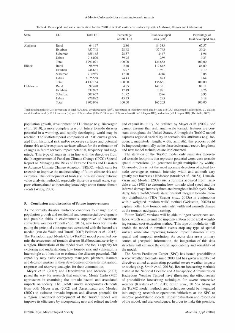
Table 4. Developed land use classification for the 2010 SERGoM raster cost surface by state (Alabama, Illinois and Oklahoma).

State LU Total HU Percentageof total HU

Total developedarea (km2)

Percentage oftotal developed area

Alabama Rural 64 197 2.80 84 383 67.57Exurban 657 708 28.68 37 763 30.24Suburban 655 165 28.57 2447 1.96Urban 916 020 39.95 289 0.23Total 2 293 091 100.00 124 882 100.00

Illinois Rural 98 969 2.40 117 642 86.09Exurban 246 661 5.97 13 931 10.19Suburban 710 965 17.20 4216 3.08Urban 3 075 558 74.43 873 0.64Total 4 132 154 100.00 136 661 100.00

Oklahoma Rural 92 420 4.85 147 321 88.11Exurban 332 987 17.49 17 991 10.76Suburban 607 657 31.92 1596 0.95Urban 870 882 45.73 295 0.18Total 1 903 946 100.00 167 203 100.00

Total housing units (HUs), percentage of total HUs, total developed area (km2), percentage of total developed area by land use (LU)-developed classification. LU classesare defined as rural (>16.18 hectares (ha) per HU); exurban (0.8–16.18 ha per HU); suburban (0.1–0.8 ha per HU); and urban (<0.1 ha per HU) (Theobald, 2005).

population growth, development or LU change (e.g. Bierwagenet al., 2010), a more complete grasp of future tornado disasterpotential in a warming, and rapidly developing, world may bereached. The spatiotemporal comparison of POE curves gener-ated from historical risk and/or exposure surfaces and potentialfuture risk and/or exposure surfaces allows for the estimation ofchanges in future tornado impact potential, frequency and mag-nitude. This type of analysis is in line with the directives fromthe Intergovernmental Panel on Climate Change (IPCC) SpecialReport on Managing the Risks of Extreme Events and Disastersto Advance Climate Change Adaption (SREX), which calls forresearch to improve the understanding of future climate risk andextremes. The development of tools (i.e. non-stationary extremevalue analysis methods), especially those on a small scale, sup-ports efforts aimed at increasing knowledge about future climateevents (Wilby, 2007).

5. Conclusion and discussion of future improvements

As the tornado disaster landscape continues to change due topopulation growth and residential and commercial developmentand possible shifts in environments supportive of hazardousconvective weather (Tippett et al., 2015), new tools for investi-gating the potential consequences associated with the hazard areneeded (van de Walle and Turoff, 2007; Pelletier et al., 2015).The Tornado Impact Monte Carlo (TorMC) model presented per-mits the assessment of tornado disaster likelihood and severity ina region. Illustrations of the model reveal the tool’s capacity forexploring and understanding how tornado risk and vulnerabilityintermingle at a location to estimate the disaster potential. Thiscapability may assist emergency managers, planners, insurersand decision makers in their development of disaster mitigation,response and recovery strategies for their communities.

Meyer et al. (2002) and Daneshvaran and Morden (2007)paved the way for research that employed Monte Carlo (MC)approaches in examining the tornado hazard and associatedimpacts on society. The TorMC model incorporates elementsfrom both Meyer et al. (2002) and Daneshvaran and Morden(2007) to estimate tornado impacts and disaster potential fora region. Continued development of the TorMC model willimprove its efficiency by incorporating new and refined methods

and expand its utility. As outlined by Meyer et al. (2002), onecannot assume that real, small-scale tornado features are con-stant throughout the United States. Although the TorMC modelcaptures regional variability in tornado risk attributes (e.g. fre-quency, magnitude, length, width, azimuth), this process couldbe improved potentially as the observed tornado record lengthensand new model techniques are implemented.

The iteration of the TorMC model only simulates theoreti-cal tornado footprints that represent potential worst-case tornadospatial dimensions (i.e. generated length multiplied by width).Obviously, this is not the most accurate depiction of actual tor-nado coverage as tornado intensity, width and azimuth varygreatly as it traverses a landscape (Strader et al., 2015a). Danesh-varan and Morden (2007) use a formula acquired from Twis-dale et al. (1981) to determine how tornado wind speed and theinferred damage intensity fluctuate throughout its life cycle. Sim-ilarly, future TorMC model iterations will integrate tornado inten-sity distributions (TID) (Strader et al., 2015a) in conjunctionwith a weighted ‘random walk’ method (Weisstein, 2002b) tocapture better how tornado intensity, width and azimuth changeas the tornado navigates a setting.

Future TorMC versions will be able to ingest vector cost sur-faces, which will permit the implementation of the areal weight-ing tornado cost-extraction method. This type of modularity willenable the model to simulate events atop any type of spatialsurface while also improving tornado impact estimates at anyspatial and temporal resolution. As vector data are a primarysource of geospatial information, the integration of this datastructure will enhance the overall applicability and versatility ofthe model.

The Storm Prediction Center (SPC) has issued probabilisticsevere weather forecasts since 2000 and has given a number ofdirectives aimed at estimating potential severe weather impactson society (e.g. Smith et al., 2015a). Recent forecasting methodstested at the National Oceanic and Atmospheric AdministrationHazardous Weather Testbed have illustrated the effectivenessof probabilistic forecasting techniques for severe convectiveweather (Karstens et al., 2015; Smith et al., 2015b). Many ofthe TorMC model methods and techniques could be integratedinto ongoing research-to-operations initiatives at the SPC toimprove probabilistic societal impact estimation and resolutionof the model, and user confidence. In order to make this possible,


S.M. Strader et al.

improving the functionality and accuracy of the TorMC modelfor shorter than annual time periods (i.e. seasonal, monthly,weekly and daily) is needed. Such processes will require bothsubjective user (e.g. forecaster) input and testing as well asthe continued advancement in research, employing numericalforecast guidance (e.g. proxy severe weather reports usingthe National Center for Environmental Prediction’s (NCEP)High-Resolution Rapid Refresh (HRRR) model; Trapp et al.,2011; Gensini and Mote, 2014) to approximate fine-scale, local,severe weather occurrences.

The TorMC model has a number of potential applicationsbeyond this initial investigation. The methods and techniquesused in the development of this model could be expanded to avariety of other geophysical hazards such as severe non-tornadicwind, hail, tropical cyclones, flooding, volcanic eruptions, earth-quakes, to improve the overall understanding of how these haz-ards interact with and impact society. Because of this applicabil-ity, future work regarding the TorMC model choices and impli-cations will be illustrated through a user guide or manual. Thismanual will enable users to apply the TorMC model in their ownresearch efficiently.

Models employing similar computational strategies to theTorMC may spur disaster mitigation and response strategieson the local, state and national scales. The adaption, improve-ment and enforcement of land-planning policies could increasethe resilience while reducing the hazard risk (e.g. Mann et al.,2014; IPCC, 2014). For example, the implementation of tornadosafe rooms or tornado shelters and adaption of building codesmay enhance tornado survivability and decrease disaster conse-quences in tornado-prone areas (Simmons and Sutter, 2007; Pre-vatt et al., 2012; Simmons et al., 2015). Restricting new devel-opment near uncertain and dynamic floodplains (Patterson andDoyle, 2009), seismically and volcanically active areas (Straderet al., 2015b), locations prone to wildfires (Bryant and Wester-ling, 2014; Mann et al., 2014), regions subject to tropical cyclonehazards and sea-level rise (Pielke et al., 2008; Maloney and Pre-ston, 2014) may reduce disaster losses. As decision makers,emergency managers and land use (LU) planners actively incor-porate disaster potential into their policies and strategies andinvest in those strategies, hazard impacts could be decreased andpotential disasters averted.

Acknowledgements

The authors would like to thank the anonymous reviewers whosesuggestions improved the manuscript significantly. They alsothank Dr. Andrew Krmenec and Mr. Alex Haberlie for theircomments and suggestions on earlier versions of this modeland manuscript. Lastly, the authors wish to thank Dr. DavidChangnon and the Meteorology Program/Geography Depart-ment Research Fund for supporting this research.

References

Agee E, Childs S. 2014. Adjustments in tornado counts, F-scale intensity,and path width for assessing significant tornado destruction. J. Appl.Meteorol. Climatol. 53(6): 1494–1505.

Anderson C, Wikle C, Zhou Q, Royle J. 2007. Population influenceson tornado reports in the United States. Weather Forecast. 22(3):571–579.

Apel H, Thieken A, Merz B, Blöschl G. 2004. Flood risk assessment andassociated uncertainty. Nat. Hazards Earth Syst. Sci. 4(2): 295–308.

Ashley W. 2007. Spatial and temporal analysis of tornado fatalities inthe United States: 1880–2005. Weather Forecast. 22: 1214–1228.

Ashley W, Strader S. 2015. Recipe for disaster: how the dynamic ingredi-ents of risk and exposure are changing the tornado disaster landscape.Bull. Am. Meteorol. Soc. DOI: 10.1175/BAMS-D-15-00150.1.

Ashley W, Strader S, Rosencrants T, Krmenec A. 2014. Spatiotemporalchanges in tornado hazard exposure: the case of the expanding bull’seye effect in Chicago, IL. Weather Clim. Soc. 6: 175–193.

Balk D, Brickman M, Anderson B, Pozzi F, Yetman G. 2005. Map-ping global urban and rural population distributions: Estimates offuture global population distribution to 2015. Center for Interna-tional Earth Science Information Network, Socioeconomic Data andApplications Center, Columbia University, 77 pp. http://sedac.ciesin.columbia.edu/gpw/docs/GISn.24_web_gpwAnnex.pdf (accessed 5May 2015).

Bierwagen B, Theobald D, Pyke C, Choate A, Groth P, Thomas J,et al. 2010. National housing and impervious surface scenarios forintegrated climate impact assessments. Proc. Natl. Acad. Sci. U. S. A.107(49): 20887–20892.

Bouwer L. 2011. Have disaster losses increased due to anthropogenicclimate change? Bull. Am. Meteorol. Soc. 92: 39–46.

Brooks H. 2004. On the relationship of tornado path length and width tointensity. Weather Forecast. 19: 310–319.

Brooks H, Doswell C III, Kay M. 2003. Climatological estimates of localdaily tornado probability. Weather Forecast. 18: 626–640.

Bryant B, Westerling A. 2014. Scenarios for future wildfire risk inCalifornia: links between changing demography, land use, climate,and wildfire. Environmetrics 25: 454–471.

Burkett V, Davidson M. 2012. Coastal impacts, adaptation and vul-nerability: a technical input to the 2012 National Climate Assess-ment. Cooperative Report to the 2013 National Climate Assessment,Island Press Washington, DC; 150 pp.

Changnon S, Pielke R Jr, Changnon D, Sylves R, Pulwarty R. 2000.Human factors explain the increased losses from weather and climateextremes. Bull. Am. Meteorol. Soc. 81: 437–442.

Coleman T, Dixon P. 2014. An objective analysis of tornado risk in theUnited States. Weather Forecast. 29(2): 366–376.

Cutter SL, Emrich CT, Webb JJ, Morath D. 2009. Social vulnerabilityto climate variability hazards: a review of the literature. Final Reportto Oxfam America. University of South Carolina, Columbia, SC;44 pp.

Daneshvaran S, Morden R. 2007. Tornado risk analysis in the UnitedStates. J. Risk Finance 8(2): 97–111.

Diffenbaugh N, Scherer M, Trapp R. 2013. Robust increases in severethunderstorm environments in response to greenhouse forcing. Proc.Natl. Acad. Sci. U. S. A. 110: 16361–16366.

Dixon P, Mercer A, Choi J, Allen J. 2011. Tornado risk analysis: isDixie Alley an extension of tornado alley? Bull. Am. Meteorol. Soc.92: 433–441.

Doswell C III. 2007. Small sample size and data quality issues illustratedusing tornado occurrence data. Electron. J. Severe Storms Meteorol.2(5): 1–16.

Doswell C III, Brooks H, Kay M. 2005. Climatological estimates ofdaily local nontornadic severe thunderstorm probability for the UnitedStates. Weather Forcast. 20: 577–595.

Doswell CA III, Brooks HE, Dotzek N. 2009. On the implementation ofthe Enhanced Fujita Scale in the USA. Atmos. Res. 93: 554–563

Edwards R, LaDue J, Ferree J, Scharfenberg K, Maier C, CoulbourneL. 2013. Tornado intensity estimation: past, present, and future. Bull.Am. Meteorol. Soc. 94(5): 641–653.

Efron B, Tibshirani R. 1994. An Introduction to the Bootstrap. CRCPress: Boca Raton, FL.

Farney T, Dixon P. 2014. Variability of tornado climatology across thecontinental United States. Int. J. Climatol. 35(10): 2993–3006.

Gensini V, Mote T. 2014. Estimations of hazardous convective weatherin the United States using dynamical downscaling. J. Clim. 27:6581–6598.

Gensini V, Mote T. 2015. Downscaled estimates of late 21st centurysevere weather from CCSM3. Clim. Change 129: 307–321.

Grazulis T. 1993. Significant Tornadoes, 1680–1991. EnvironmentalFilms: St. Johnsbury, VT; 1326 pp.

Huggel C, Stone D, Auffhammer M, Hansen G. 2013. Loss and damageattribution. Nat. Clim. Change 3: 694–696.

IPCC. 2014. Climate change 2014: mitigation of climate change.Contribution of Working Group III to the Fifth Assessment.Report of the Intergovernmental Panel on Climate Change. IPCC.http://www.ipcc.ch/report/ar5/syr/ (accessed 1 June 2015)

Karstens C, Stumpf G, Ling C, Hua L, Kingfield D, Smith T, et al.2015. Evaluation of a probabilistic forecasting methodology for severeconvective weather in the 2014 hazardous weather testbed. WeatherForecast. 3: 1551–1570, DOI: 10.1175/WAF-D-14-00163.1.



Kunkel K, Karl T, Brooks H, Kossin J, Lawrimore J, Arndt D, et al.2013. Monitoring and understanding trends in extreme storms: stateof knowledge. Bull. Am. Meteorol. Soc. 94(4): 499–514.

Maloney M, Preston B. 2014. A geospatial dataset for U.S. hurricanestorm surge and sea-level rise vulnerability: development and casestudy applications. Clim. Risk Manage. 2: 26–41.

Mann M, Berck P, Moritz M, Batllori E, Baldwin J, Gately C, et al. 2014.Modeling residential development in California from 2000 to 2050:integrating wildfire risk, wildland and agricultural encroachment.Land Use Policy 41: 438–452.

Meyer C, Brooks H, Kay M. 2002. A hazard model for tornado occur-rence in the United States. Extended Abstracts, In American Mete-orological Society 13th Symposium on Global Change and ClimateVariations, January 13–17, Orlando, FL.

Mooney C. 1997. Monte Carlo Simulation, Vol. 116. Sage Publications:Thousand Oaks, CA.

Morss R, Wilhelmi O, Meehl G, Dilling L. 2011. Improving societaloutcomes of extreme weather in a changing climate: an integratedperspective. Ann. Rev. Environ. Resour. 36: 1–25.

Nicholls RJ, Small C. 2002. Improved estimates of coastal populationand exposure to hazards released. Eos Trans. AGU 83: 301–305.

Patterson L, Doyle M. 2009. Assessing effectiveness of national floodpolicy through spatiotemporal monitoring of socioeconomic exposure.J. Am. Water Resour. Assoc. 45: 237–252.

Pelletier J, Murray B, Pierce J, Bierman P, Breshears D, Crosby B, et al.2015. Forecasting the response of Earth’s surface to future climaticand land-use changes: a review of methods and research needs. Earth’sFuture 3: 220–251.

Petersen A. 2012. Simulating Nature: A Philosophical Study ofComputer-Simulation Uncertainties and Their Role in ClimateScience and Policy Advice. CRC Press: London, UK.

Pielke R Jr. 2005. Attribution of disaster losses. Science 311:1615–1616.

Pielke R Jr, Gratz J, Landsea C, Collins D, Saunders M, Musulin R. 2008.Normalized hurricane damage in the United States: 1900–2005. Nat.Hazards Rev. 9: 29–42.

Prevatt D, van de Lindt J, Back E, Graettinger A, Pei S, Coulbourne W,et al. 2012. Making the case for improved structural design: tornadooutbreaks of 2011. Leadership Manage. Eng. 12: 254–270.

Rae S, Stefkovich J. 2000. The tornado damage risk assessment pre-dicting the impact of a big outbreak in Dallas–Fort Worth, Texas.Extended Abstracts. In 20th Conference on Severe Local Storms.American Meteorological Society, Orlando, FL.

Rahman A, Weinmann P, Hoang T, Laurenson E. 2002. Monte Carlosimulation of flood frequency curves from rainfall. J. Hydrol. 256(3):196–210.

Rosencrants T, Ashley W. 2015. Spatiotemporal analysis of tornadoexposure in five U.S. metropolitan areas. Nat. Hazards 78: 121–140.

Schlossberg M. 2003. GIS, the US Census and neighbourhood scaleanalysis. Plan. Practice Res. 18: 213–217.

SEDAC. 2015. U.S. Census grids. Socioeconomic Data and ApplicationsCenter, Columbia University. http://sedac.ciesin.columbia.edu/usgrid/(accessed 15 June 2015)

Simmons K, Kovacs P, Kopp G. 2015. Tornado damage mitigation: ben-efit/cost analysis of enhanced building codes in Oklahoma. WeatherClim. Soc. 7: 169–178, DOI: 10.1175/WCAS-D-14-00032.1.

Simmons K, Sutter D. 2007. Tornado shelters and the housing market.Constr. Manage. Econ. 25: 1119–1126.

Smith B, Dean A, Thompson R, Leitman, E, Grams, J. 2015b. Devel-opmental work at the Storm Prediction Center in pursuit of tornadicsupercell probability and tornado Intensity estimation using a severesupercell dataset. In 2015 NWA Meeting, 17–22 October 2015, Okla-homa City, OK.

Smith A, Katz R. 2013. US billion-dollar weather and climate disas-ters: data sources, trends, accuracy and biases. Nat. Hazards 7(2):387–410.

Smith B, Thompson R, Dean A, Marsh P. 2015a. Diagnosing the condi-tional probability of tornado damage rating using environmental andradar attributes. Weather Forecast. 30: 914–932.

Smith B, Thompson R, Grams J, Broyles C, Brooks H. 2012. Convectivemodes for significant severe thunderstorms in the contiguous UnitedStates. Part I: storm classification and climatology. Weather Forecast.27(5): 1114–1135.

Strader S, Ashley W. 2015. The expanding bull’s eye effect. Weatherwise68(5): 23–29.

Strader S, Ashley W, Irizarry A, Hall S. 2015a. A climatology of tornadointensity assessments. Meteorol. Appl. 22: 1365–1392.

Strader S, Ashley W, Walker J. 2015b. Changes in volcanic hazardexposure in the Northwest USA from 1940 to 2100. Nat. Hazards 77:1365–1392.

Suckling P, Ashley W. 2006. Spatial and temporal characteristics oftornado path direction. Prof. Geogr. 58: 20–38.

Theobald D. 2005. Landscape patterns of exurban growth in theUSA from 1980 to 2020. Ecol. Soc. 10(32). http://www.tetonwyo.org/compplan/LDRUpdate/RuralAreas/Additional%20Resources/Theobald2005.pdf (accessed 2 February 2015)

Thorne P, Vose R. 2010. Reanalysis suitable for characterizing long-termtrends: are they really achievable? Bull. Am. Meteorol. Soc. 91:353–361.

Tippett M, Allen J, Gensini V, Brooks H. 2015. Climate and hazardousconvective weather. Curr. Clim. Change Rep. 1(2): 60–73.

Trapp R, Diffenbaugh N, Brooks H, Baldwin M, Robinson E, Pal J. 2007.Changes in severe thunderstorm environment frequency during the21st century caused by anthropogenically enhanced global radiativeforcing. Proc. Natl. Acad. Sci. U. S. A. 104: 19719–19723.

Trapp R, Robinson E, Baldwin M, Diffenbaugh N, Schwedler B.2011. Regional climate of hazardous convective weather throughhigh-resolution dynamical downscaling. Clim. Dyn. 37: 677–688.

Twisdale L, Dunn W, Davis T, Horie Y. 1981. Tornado missile simula-tion and design methodology. EPRI NP-2005, EPRI: Palo Alto, CA.

Van de Walle B, Turoff M. 2007. Emergency response informationsystems: emerging trends and technologies. Commun. ACM 50(3):29–31.

Verbout S, Brooks H, Leslie L, Schultz D. 2006. Evolution of the U.S.Tornado database: 1954–2003. Weather Forecast. 21: 86–93.

Weisstein E. 2002a. Sphere point picking. MathWorld – a Wolfram webresource. http://mathworld.wolfram.com/SpherePointPicking.html(accessed 21 May 2015).

Weisstein E. 2002b. Random walk – 1-dimensional. MathWorld – aWolfram web resource. http://mathworld.wolfram.com/RandomWalk1-Dimensional.html (accessed 21 May 2015).

Wilby R. 2007. A review of climate change impacts on the built environ-ment. Built Environ. 33(1): 31–45.

Wurman J, Robinson P, Alexander C, Richardson Y. 2007. Low-levelwinds in tornadoes and potential catastrophic tornado impacts in urbanareas. Bull. Am. Meteorol. Soc. 88(1): 31–46.


Documents

A Monte Carlo model for estimating tornado impacts