1

A Multi-core High Performance ComputingFramework for Probabilistic Solutions of

Distribution SystemsTao Cui, Student Member, IEEE, Franz Franchetti, Member, IEEE

Abstract—Multi-core CPUs with multiple levels of parallelismand deep memory hierarchies have become the mainstreamcomputing platform. In this paper we developed a generallyapplicable high performance computing framework for MonteCarlo simulation (MCS) type applications in distribution sys-tems, taking advantage of performance-enhancing features ofmulti-core CPUs. The application in this paper is to solve theprobabilistic load flow (PLF) in real time, in order to cope withthe uncertainties caused by the integration of renewable energyresources. By applying various performance optimizations andmulti-level parallelization, the optimized MCS solver is able toachieve more than 50% of a CPU’s theoretical peak performanceand the performance is scalable with the hardware parallelism.We tested the MCS solver on the IEEE 37-bus test feeder usinga new Intel Sandy Bridge multi-core CPU. The optimized MCSsolver is able to solve millions of load flow cases within a second,enabling the real-time Monte Carlo solution of the PLF.

Index Terms—Distribution systems, high performance comput-ing, Monte Carlo simulation, probabilistic load flow, renewableenergy integration.

I. INTRODUCTION

The integration of renewable energy resources such as

wind and solar energy in distribution systems introduces

significant uncertainties. A fast and generally applicable com-

puting framework that can assess system states in real time

considering the impact of such large uncertainties would be

an important tool for the reliable operation of distribution

systems. In this paper, we developed a multi-core high perfor-

mance computing framework for fast Monte Carlo simulation

(MCS) of distribution networks, with focus on leveraging the

capabilities of modern multicore CPUs. The target application

is to solve the distribution system probabilistic load flows

(PLF) in real time, in order to monitor and assess the system

states given the probabilistic properties of the uncertainties.

The probabilistic load flow (PLF) models the uncertainties

as input random variables (RV) with probabilistic density

functions (PDF). Based on load flow equations, it computes

the output states as random variables with PDFs [1] [2]. The

solution methods for PLF generally fall into two categories: the

analytical methods and MCS based methods. Most analytical

methods are trying to compute the output RVs by simplifying

power system models or probabilistic models [2] [3] [4] [5].

However, due to the simplification, analytical methods may not

be able to handle uncertainties with large variance or systems

This work was supported by NSF through awards 0931978 and 0702386.T. Cui and F. Franchetti are with the Department of Electrical and Computer

Engineering, Carnegie Mellon University, Pittsburgh, PA, 15213 USA. e-mail:{tcui,franzf}@ece.cmu.edu

with large non-linearity. MCS is a general framework extensi-

ble for many statistical applications including solving PLF. It

samples the input RVs and solves load flow for each sample

using the accurate system model without simplifications, and

then estimates the output RVs using all result samples. The

accuracy and convergence of MCS are guaranteed by the Law

of Large Number [6]. Therefore, the MCS solutions are often

used as accuracy references for most PLF researches and

applications [2] [4] [7]. In order to obtain accurate results,

the MCS needs to solve a large number of load flows, due to

the computational burden, MCS methods are often believed to

be prohibitive and infeasible for real-time applications.

The performance capabilities of modern computing plat-

forms have been growing rapidly in last several decades

at a roughly exponential rate [8] [9]. The new mainstream

multi-core CPUs and graphics cards (GPUs) enable us to

build inexpensive systems with computational power similar

to supercomputers about a decade ago [8]. However, it is

very difficult to fully utilize the hardware computing power

for specific application. It requires the knowledge from both

application domain and computer architecture domain and

extensive program optimization.

Contribution. In [10], we presented an initial version of

a high performance solver for distribution system load flow

on multi-core CPUs. In this paper, we extended the work

in [10] by applying more aggressive algorithm level and

source code level optimization. Further, we demonstrate that

code optimization techniques on multi-core CPUs can yield

a significant speedup and make MCS possible and practical

for certain real-time applications. By applying various code

optimization techniques and multilevel parallelization, for the

MCS type applications, our optimized load flow solver is able

to achieve more than 50% of a CPU’s theoretical peak per-

formance. This translates into about 50x speedup comparing

to the best compiler-optimized baseline code on a quad-core

CPU. The performance is also scalable with the hardware’s

parallel capabilities (multiple cores and SIMD vector width).

We further implemented a task-decomposition based threading

structure for real-time MCS based PLF application including

parallel random number generator, load flow solver, PDF

estimation and visualization.

Synopsis. The paper is organized as follows: Multicore

CPUs and PLF approaches are reviewed in Section II. Perfor-

mance optimization methods are described in Section III. In

Section IV, we report the performance results of the optimized

solver on IEEE 4-bus system (expanded to 8192 buses) and

IEEE 37-bus system, the numeric results of the PLF solver are

in Section V.

2

II. MULTICORE PLATFORM AND PLF APPROACHES

A. Multi-core Computing Platform

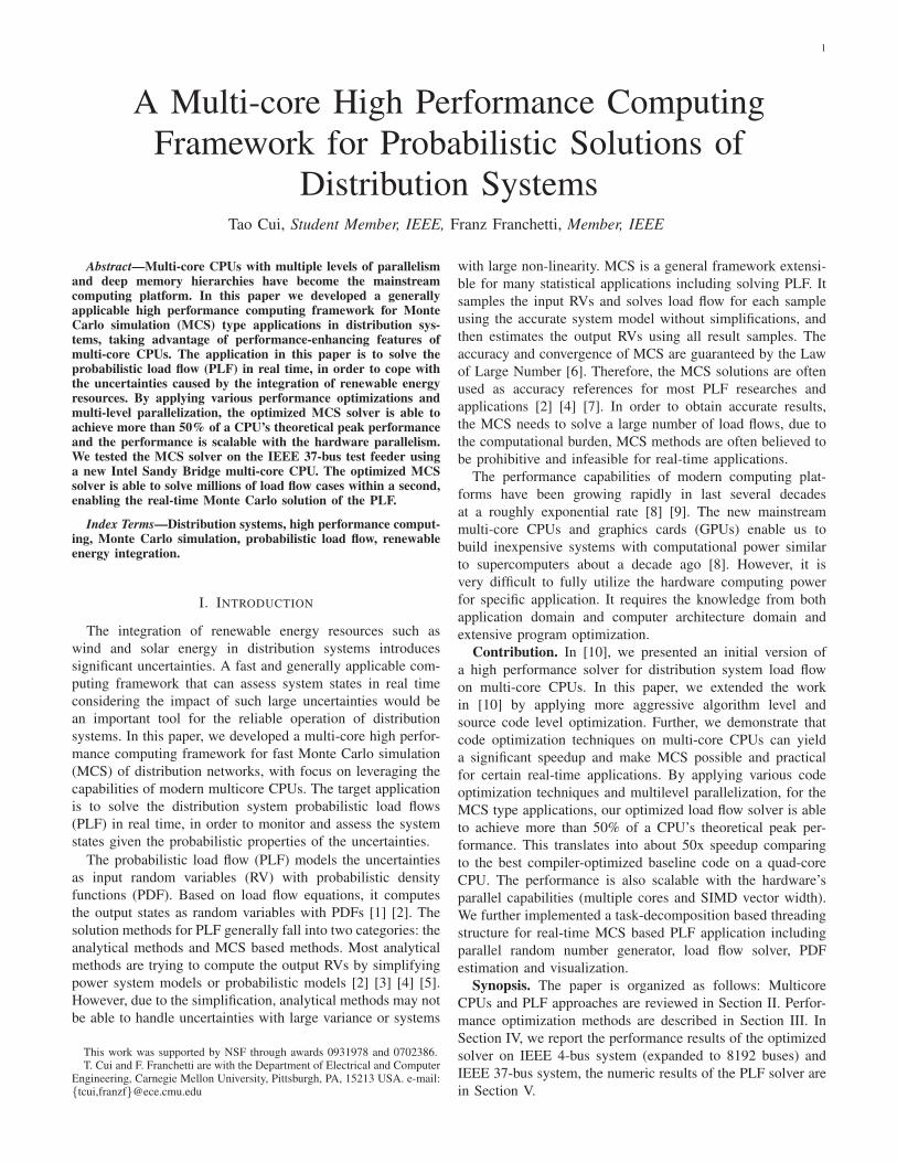
Fig. 1 shows the structure of the 6-core Intel Xeon X5680

CPU in 2010. Its theoretical peak performance is 162 Gflop/s

(1 Gflop/s = 109 floating point operations per second) [11].

This single chip desktop CPU has similar peak performance

as the fastest supercomputer (Fujitsu NWT, 236 Gflop/s) in

1995 and the 500th fastest supercomputer (Cray T3E1200, 139

Gflop/s) in 2001 [8]. However, as the computer architecture

becomes much more complicated, to fully exact performance

from the hardware architecture is very difficult. It requires

knowledge and effort from both the application domain and

the computer architecture domain, including algorithm level

optimization, data structure optimization, utilization of special

instructions, and multi-threading. The specific numerical ap-

plication needs to be carefully redesigned and tuned to fit into

the hardware. For the MCS solver, we mainly look into the

following aspects:

Main Memory (>8GB)

Multi−core CPU

L3 (12MB)

L2 (256KB) L2 (256KB) L2 (256KB) L2 (256KB) L2 (256KB)L2 (256KB)

L1 (32KB) L1 (32KB) L1 (32KB) L1 (32KB) L1 (32KB) L1 (32KB)

Core #0 Core #1 Core #2 Core #3 Core #4 Core #5

PU #0

PU #1

PU #2

PU #3

PU #4

PU #5

PU #6

PU #7

PU #8

PU #9

PU #10

PU #11

Fig. 1. Xeon X5680 CPU system structure: 6 physical cores

Memory hierarchy including multiple levels of caches. The

cache is a small but fast memory that automatically keeps

and manages copies of the most recently used and the most

adjacent data from the main memory locations in order to

bridge the speed gap between fast processor and slow main

memories. There could be multiple levels of caches: in Fig. 1,

X5680 has 3 level caches (L1,L2 and L3), the cache levels that

are closer to CPU cores are faster in speed but smaller in size.

An optimized data storage and access pattern is important to

utilize the cache functions to increase the performance.

Multiple levels of parallelism have become the major

driving force for the hardware performance. We are looking

into following aspects that are explicitly available for the

software: 1) Single Instruction Multiple Data (SIMD) uses

special instructions and registers to perform same operation on

multiple data at the same time. 2) Multithreading on multiple

CPU cores enables multiple threads to be executed simul-

taneously and independently. The MCS can be a well fitted

program model for such parallel instructions and structures.

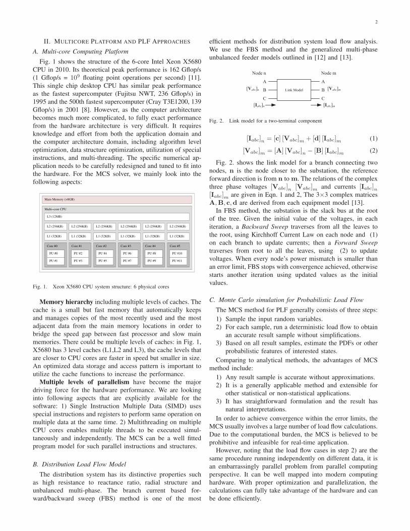
B. Distribution Load Flow Model

The distribution system has its distinctive properties such

as high resistance to reactance ratio, radial structure and

unbalanced multi-phase. The branch current based for-

ward/backward sweep (FBS) method is one of the most

efficient methods for distribution system load flow analysis.

We use the FBS method and the generalized multi-phase

unbalanced feeder models outlined in [12] and [13].

Link Model

Node n Node m

A

B

C

A

B

C

[Vabc]n [Vabc]m

[Iabc]m[Iabc]n

Fig. 2. Link model for a two-terminal component

[Iabc]n = [c] [Vabc]m + [d] [Iabc]m (1)

[Vabc]m = [A] [Vabc]n − [B] [Iabc]m (2)

Fig. 2. shows the link model for a branch connecting two

nodes, n is the node closer to the substation, the reference

forward direction is from n to m. The relations of the complex

three phase voltages [Vabc]n [Vabc]m and currents [Iabc]n[Iabc]m are given in Eqn. 1 and 2, The 3×3 complex matrices

A,B, c,d are derived from each equipment model [13].

In FBS method, the substation is the slack bus at the root

of the tree. Given the initial value of the voltages, in each

iteration, a Backward Sweep traverses from all the leaves to

the root, using Kirchhoff Current Law on each node and (1)

on each branch to update currents; then a Forward Sweeptraverses from root to all the leaves, using (2) to update

voltages. When every node’s power mismatch is smaller than

an error limit, FBS stops with convergence achieved, otherwise

starts another iteration using updated values as the initial

values.

C. Monte Carlo simulation for Probabilistic Load Flow

The MCS method for PLF generally consists of three steps:

1) Sample the input random variables.

2) For each sample, run a deterministic load flow to obtain

an accurate result sample without simplifications.

3) Based on all result samples, estimate the PDFs or other

probabilistic features of interested states.

Comparing to analytical methods, the advantages of MCS

method include:

1) Any result sample is accurate without approximations.

2) It is a generally applicable method and extensible for

other statistical or non-statistical applications.

3) It has straightforward formulation and the result has

natural interpretations.

In order to achieve convergence within the error limits, the

MCS usually involves a large number of load flow calculations.

Due to the computational burden, the MCS is believed to be

prohibitive and infeasible for real-time application.

However, noting that the load flow cases in step 2) are the

same procedure running independently on different data, it is

an embarrassingly parallel problem from parallel computing

perspective. It can be well mapped into modern computing

hardware. With proper optimization and parallelization, the

calculations can fully take advantage of the hardware and can

be done efficiently.

3

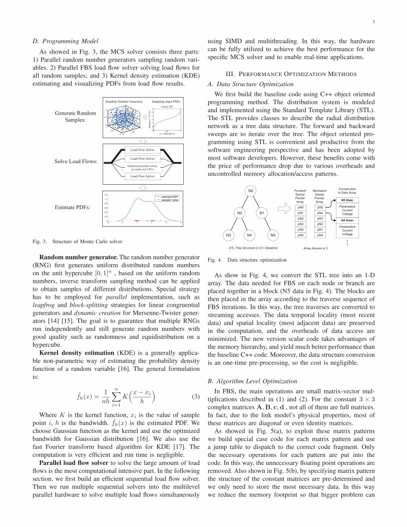
D. Programming Model

As showed in Fig. 3, the MCS solver consists three parts:

1) Parallel random number generators sampling random vari-

ables. 2) Parallel FBS load flow solver solving load flows for

all random samples; and 3) Kernel density estimation (KDE)

estimating and visualizing PDFs from load flow results.

-10 -5 0 5 10 150

0.02

0.04

0.06

0.08

0.1

0.12

estimated PDFsamples' value

Load Flow Solver

Load Flow Solver

Load Flow Solver

00.5

1

0

0.5

10

0.5

1

Generate Random Samples:

Solve Load Flows:

Estimate PDFs:

Optimized parallel solvers on multi-core CPUs

Random Number Generator Sampling input PDFs

......

......

0 0.5 1-3

-2

-1

0

1

2

3Inverse CDF

Sam

ple

X =

F-1

(U)

U ~ Uniform[0,1]

Fig. 3. Structure of Monte Carlo solver

Random number generator. The random number generator

(RNG) first generates uniform distributed random numbers

on the unit hypercube [0, 1]n , based on the uniform random

numbers, inverse transform sampling method can be applied

to obtain samples of different distributions. Special strategy

has to be employed for parallel implementation, such as

leapfrog and block-splitting strategies for linear congruential

generators and dynamic creation for Mersenne-Twister gener-

ators [14] [15]. The goal is to guarantee that multiple RNGs

run independently and still generate random numbers with

good quality such as randomness and equidistribution on a

hypercube.

Kernel density estimation (KDE) is a generally applica-

ble non-parametric way of estimating the probability density

function of a random variable [16]. The general formulation

is:

fh(x) =1

nh

n∑i=1

K(x− xi

h

)(3)

Where K is the kernel function, xi is the value of sample

point i, h is the bandwidth. fh(x) is the estimated PDF. We

choose Gaussian function as the kernel and use the optimized

bandwidth for Gaussian distribution [16]. We also use the

fast Fourier transform based algorithm for KDE [17]. The

computation is very efficient and run time is negligible.

Parallel load flow solver to solve the large amount of load

flows is the most computational intensive part. In the following

section, we first build an efficient sequential load flow solver.

Then we run multiple sequential solvers into the multilevel

parallel hardware to solve multiple load flows simultaneously

using SIMD and multithreading. In this way, the hardware

can be fully utilized to achieve the best performance for the

specific MCS solver and to enable real-time applications.

III. PERFORMANCE OPTIMIZATION METHODS

A. Data Structure Optimization

We first build the baseline code using C++ object oriented

programming method. The distribution system is modeled

and implemented using the Standard Template Library (STL).

The STL provides classes to describe the radial distribution

network as a tree data structure. The forward and backward

sweeps are to iterate over the tree. The object oriented pro-

gramming using STL is convenient and productive from the

software engineering perspective and has been adopted by

most software developers. However, these benefits come with

the price of performance drop due to various overheads and

uncontrolled memory allocation/access patterns.

N0

N2 N1

N3 N4 N5

pN0

pN1

pN2

pN3

pN4

Forward SweepPointer Array

pN5

pN5

pN4

pN3

pN2

pN1

Backward SweepPointer Array

pN0

STL Tree Structure in C++ Baseline Array Access in C

N5 Data:

ParametersCurrentVoltage

N4 Data:

ParametersCurrentVoltage

Consecutive in Data Array

...

Fig. 4. Data structure optimization

As show in Fig. 4, we convert the STL tree into an 1-D

array. The data needed for FBS on each node or branch are

placed together in a block (N5 data in Fig. 4). The blocks are

then placed in the array according to the traverse sequence of

FBS iterations. In this way, the tree traverses are converted to

streaming accesses. The data temporal locality (most recent

data) and spatial locality (most adjacent data) are preserved

in the computation, and the overheads of data access are

minimized. The new version scalar code takes advantages of

the memory hierarchy, and yield much better performance than

the baseline C++ code. Moreover, the data structure conversion

is an one-time pre-processing, so the cost is negligible.

B. Algorithm Level Optimization

In FBS, the main operations are small matrix-vector mul-

tiplications described in (1) and (2). For the constant 3 × 3complex matrices A,B, c,d , not all of them are full matrices.

In fact, due to the link model’s physical properties, most of

these matrices are diagonal or even identity matrices.

As showed in Fig. 5(a), to exploit these matrix patterns

we build special case code for each matrix pattern and use

a jump table to dispatch to the correct code fragment. Only

the necessary operations for each pattern are put into the

code. In this way, the unnecessary floating point operations are

removed. Also shown in Fig. 5(b), by specifying matrix pattern

the structure of the constant matrices are pre-determined and

we only need to store the most necessary data. In this way

we reduce the memory footprint so that bigger problem can

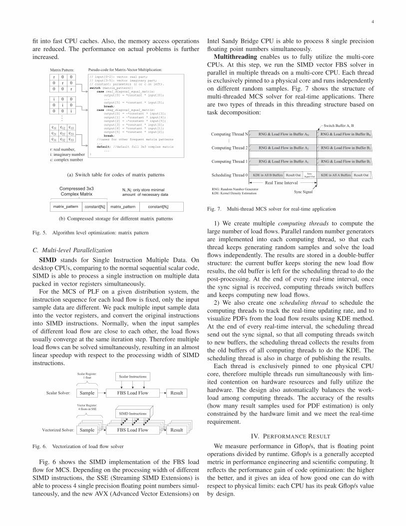
4

fit into fast CPU caches. Also, the memory access operations

are reduced. The performance on actual problems is further

increased.

// input[0~2]: vector real part; // input[3~5]: vector imaginary part;// constant: parameters (r or c on left).switch (matrix_pattern){

case real_diagonal_equal_matrix:output[0] = *constant * input[0];... output[5] = *constant * input[5];break;

case imag_diagonal_equal_matrix:output[0] = -*constant * input[3];output[1] = -*constant * input[4];output[2] = -*constant * input[5];output[3] = *constant * input[0];output[4] = *constant * input[1];output[5] = *constant * input[2];break;

//cases for other frequent matrix patterns...default: //default full 3x3 complex matrix

...}

r 0 00 r 00 0 r

i 0 00 i 00 0 i

c11 c12 c13

c21 c22 c23

c31 c32 c33

r: real number, i: imaginary numberc: complex number

...

Matrix Pattern: Pseudo-code for Matrix-Vector Multiplication:

(a) Switch table for codes of matrix patterns

matrix_pattern

Compressed 3x3 Complex Matrix

constant[Ni] constant[Nj]matrix_pattern

Ni ,Nj: only store minimal amount of necessary data

(b) Compressed storage for different matrix patterns

Fig. 5. Algorithm level optimization: matrix pattern

C. Multi-level ParallelizationSIMD stands for Single Instruction Multiple Data. On

desktop CPUs, comparing to the normal sequential scalar code,

SIMD is able to process a single instruction on multiple data

packed in vector registers simultaneously.For the MCS of PLF on a given distribution system, the

instruction sequence for each load flow is fixed, only the input

sample data are different. We pack multiple input sample data

into the vector registers, and convert the original instructions

into SIMD instructions. Normally, when the input samples

of different load flow are close to each other, the load flows

usually converge at the same iteration step. Therefore multiple

load flows can be solved simultaneously, resulting in an almost

linear speedup with respect to the processing width of SIMD

instructions.

Sample FBS Load Flow Result

Sample FBS Load Flow Result

SIMD Instructions

Scalar Instructions

Scalar Solver:

Vectorized Solver:

Vector Register: 4 floats in SSE

Scalar Register:1 float

Fig. 6. Vectorization of load flow solver

Fig. 6 shows the SIMD implementation of the FBS load

flow for MCS. Depending on the processing width of different

SIMD instructions, the SSE (Streaming SIMD Extensions) is

able to process 4 single precision floating point numbers simul-

taneously, and the new AVX (Advanced Vector Extensions) on

Intel Sandy Bridge CPU is able to process 8 single precision

floating point numbers simultaneously.

Multithreading enables us to fully utilize the multi-core

CPUs. At this step, we run the SIMD vector FBS solver in

parallel in multiple threads on a multi-core CPU. Each thread

is exclusively pinned to a physical core and runs independently

on different random samples. Fig. 7 shows the structure of

multi-threaded MCS solver for real-time applications. There

are two types of threads in this threading structure based on

task decomposition:

RNG & Load Flow in Buffer AN

RNG & Load Flow in Buffer A2

RNG & Load Flow in Buffer A1

Real Time Interval

Scheduling Thread 0

Computing Thread 2

Computing Thread 1

Computing Thread N

Sync Signal

KDE in All B Buffers Result Out

RNG & Load Flow in Buffer BN

RNG & Load Flow in Buffer B2

RNG & Load Flow in Buffer B1

Sync Signal Out

Switch Buffer A, B

KDE in All A Buffers Result Out

RNG: Random Number GeneratorKDE: Kernel Density Estimation

...

Fig. 7. Multi-thread MCS solver for real-time application

1) We create multiple computing threads to compute the

large number of load flows. Parallel random number generators

are implemented into each computing thread, so that each

thread keeps generating random samples and solve the load

flows independently. The results are stored in a double-buffer

structure: the current buffer keeps storing the new load flow

results, the old buffer is left for the scheduling thread to do the

post-processing. At the end of every real-time interval, once

the sync signal is received, computing threads switch buffers

and keeps computing new load flows.

2) We also create one scheduling thread to schedule the

computing threads to track the real-time updating rate, and to

visualize PDFs from the load flow results using KDE method.

At the end of every real-time interval, the scheduling thread

send out the sync signal, so that all computing threads switch

to new buffers, the scheduling thread collects the results from

the old buffers of all computing threads to do the KDE. The

scheduling thread is also in charge of publishing the results.

Each thread is exclusively pinned to one physical CPU

core, therefore multiple threads run simultaneously with lim-

ited contention on hardware resources and fully utilize the

hardware. The design also automatically balances the work-

load among computing threads. The accuracy of the results

(how many result samples used for PDF estimation) is only

constrained by the hardware limit and we meet the real-time

requirement.

IV. PERFORMANCE RESULT

We measure performance in Gflop/s, that is floating point

operations divided by runtime. Gflop/s is a generally accepted

metric in performance engineering and scientific computing. It

reflects the performance gain of code optimization: the higher

the better, and it gives an idea of how good one can do with

respect to physical limits: each CPU has its peak Gflop/s value

by design.

5

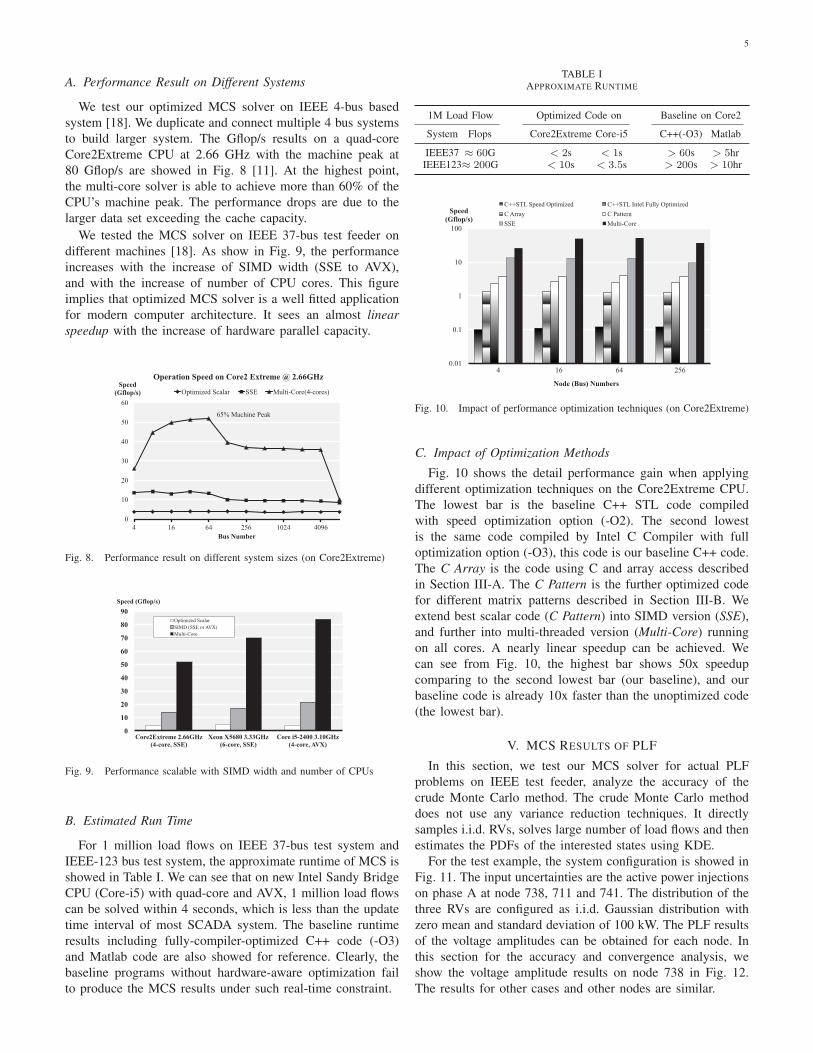
A. Performance Result on Different Systems

We test our optimized MCS solver on IEEE 4-bus based

system [18]. We duplicate and connect multiple 4 bus systems

to build larger system. The Gflop/s results on a quad-core

Core2Extreme CPU at 2.66 GHz with the machine peak at

80 Gflop/s are showed in Fig. 8 [11]. At the highest point,

the multi-core solver is able to achieve more than 60% of the

CPU’s machine peak. The performance drops are due to the

larger data set exceeding the cache capacity.

We tested the MCS solver on IEEE 37-bus test feeder on

different machines [18]. As show in Fig. 9, the performance

increases with the increase of SIMD width (SSE to AVX),

and with the increase of number of CPU cores. This figure

implies that optimized MCS solver is a well fitted application

for modern computer architecture. It sees an almost linearspeedup with the increase of hardware parallel capacity.

0

10

20

30

40

50

60

4 16 64 256 1024 4096

Speed (Gflop/s)

Bus Number

Operation Speed on Core2 Extreme @ 2.66GHz

Optimized Scalar SSE Multi-Core(4-cores)

65% Machine Peak

Fig. 8. Performance result on different system sizes (on Core2Extreme)

0

10

20

30

40

50

60

70

80

90

Core2Extreme 2.66GHz (4-core, SSE)

Xeon X5680 3.33GHz (6-core, SSE)

Core i5-2400 3.10GHz (4-core, AVX)

Speed (Gflop/s)

Optimized Scalar SIMD (SSE or AVX) Multi-Core

Fig. 9. Performance scalable with SIMD width and number of CPUs

B. Estimated Run Time

For 1 million load flows on IEEE 37-bus test system and

IEEE-123 bus test system, the approximate runtime of MCS is

showed in Table I. We can see that on new Intel Sandy Bridge

CPU (Core-i5) with quad-core and AVX, 1 million load flows

can be solved within 4 seconds, which is less than the update

time interval of most SCADA system. The baseline runtime

results including fully-compiler-optimized C++ code (-O3)

and Matlab code are also showed for reference. Clearly, the

baseline programs without hardware-aware optimization fail

to produce the MCS results under such real-time constraint.

TABLE IAPPROXIMATE RUNTIME

1M Load Flow Optimized Code on Baseline on Core2

System Flops Core2Extreme Core-i5 C++(-O3) Matlab

IEEE37 ≈ 60G < 2s < 1s > 60s > 5hrIEEE123≈ 200G < 10s < 3.5s > 200s > 10hr

0.01

0.1

1

10

100

4 16 64 256

Speed (Gflop/s)

C++STL Speed Optimized C++STL Intel Fully Optimized C Array C Pattern SSE Multi-Core

Node (Bus) Numbers

Fig. 10. Impact of performance optimization techniques (on Core2Extreme)

C. Impact of Optimization Methods

Fig. 10 shows the detail performance gain when applying

different optimization techniques on the Core2Extreme CPU.

The lowest bar is the baseline C++ STL code compiled

with speed optimization option (-O2). The second lowest

is the same code compiled by Intel C Compiler with full

optimization option (-O3), this code is our baseline C++ code.

The C Array is the code using C and array access described

in Section III-A. The C Pattern is the further optimized code

for different matrix patterns described in Section III-B. We

extend best scalar code (C Pattern) into SIMD version (SSE),

and further into multi-threaded version (Multi-Core) running

on all cores. A nearly linear speedup can be achieved. We

can see from Fig. 10, the highest bar shows 50x speedup

comparing to the second lowest bar (our baseline), and our

baseline code is already 10x faster than the unoptimized code

(the lowest bar).

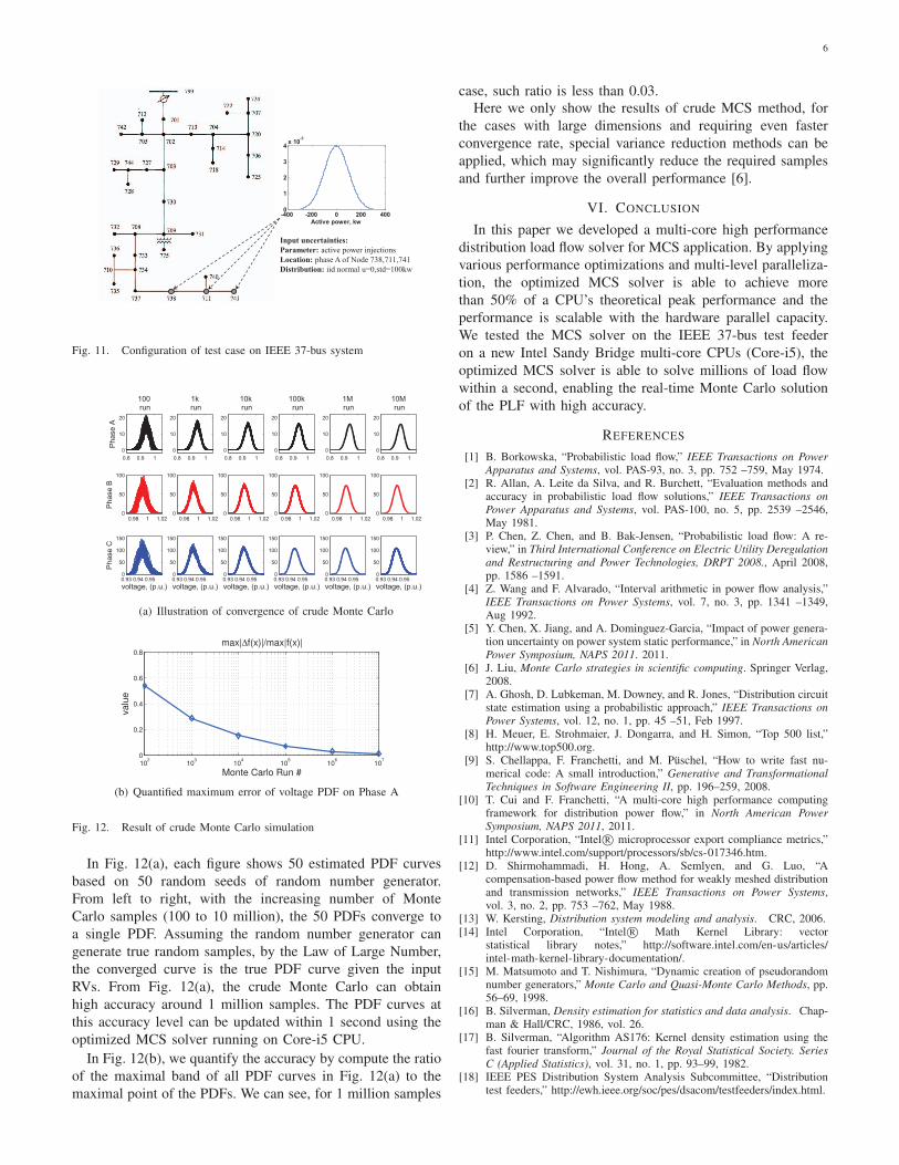
V. MCS RESULTS OF PLF

In this section, we test our MCS solver for actual PLF

problems on IEEE test feeder, analyze the accuracy of the

crude Monte Carlo method. The crude Monte Carlo method

does not use any variance reduction techniques. It directly

samples i.i.d. RVs, solves large number of load flows and then

estimates the PDFs of the interested states using KDE.

For the test example, the system configuration is showed in

Fig. 11. The input uncertainties are the active power injections

on phase A at node 738, 711 and 741. The distribution of the

three RVs are configured as i.i.d. Gaussian distribution with

zero mean and standard deviation of 100 kW. The PLF results

of the voltage amplitudes can be obtained for each node. In

this section for the accuracy and convergence analysis, we

show the voltage amplitude results on node 738 in Fig. 12.

The results for other cases and other nodes are similar.

6

-400 -200 0 200 4000

1

2

3

4 x 10-3

Active power, kw

Input uncertainties: Parameter: active power injectionsLocation: phase A of Node 738,711,741Distribution: iid normal u=0,std=100kw

Fig. 11. Configuration of test case on IEEE 37-bus system

0.8 0.9 10

10

20

100 run

Pha

se A

0.98 1 1.020

50

100

Pha

se B

0.93 0.94 0.950

50

100

150

Pha

se C

voltage, (p.u.)

0.8 0.9 10

10

20

1k run

0.98 1 1.020

50

100

0.93 0.94 0.950

50

100

150

voltage, (p.u.)

0.8 0.9 10

10

20

10k run

0.98 1 1.020

50

100

0.93 0.94 0.950

50

100

150

voltage, (p.u.)

0.8 0.9 10

10

20

100k run

0.98 1 1.020

50

100

0.93 0.94 0.950

50

100

150

voltage, (p.u.)

0.8 0.9 10

10

20

1M run

0.98 1 1.020

50

100

0.93 0.94 0.950

50

100

150

voltage, (p.u.)

0.8 0.9 10

10

20

10M run

0.98 1 1.020

50

100

0.93 0.94 0.950

50

100

150

voltage, (p.u.)

(a) Illustration of convergence of crude Monte Carlo

102

103

104

105

106

107

0

0.2

0.4

0.6

0.8

Monte Carlo Run #

max|Δf(x)|/max|f(x)|

valu

e

(b) Quantified maximum error of voltage PDF on Phase A

Fig. 12. Result of crude Monte Carlo simulation

In Fig. 12(a), each figure shows 50 estimated PDF curves

based on 50 random seeds of random number generator.

From left to right, with the increasing number of Monte

Carlo samples (100 to 10 million), the 50 PDFs converge to

a single PDF. Assuming the random number generator can

generate true random samples, by the Law of Large Number,

the converged curve is the true PDF curve given the input

RVs. From Fig. 12(a), the crude Monte Carlo can obtain

high accuracy around 1 million samples. The PDF curves at

this accuracy level can be updated within 1 second using the

optimized MCS solver running on Core-i5 CPU.

In Fig. 12(b), we quantify the accuracy by compute the ratio

of the maximal band of all PDF curves in Fig. 12(a) to the

maximal point of the PDFs. We can see, for 1 million samples

case, such ratio is less than 0.03.Here we only show the results of crude MCS method, for

the cases with large dimensions and requiring even faster

convergence rate, special variance reduction methods can be

applied, which may significantly reduce the required samples

and further improve the overall performance [6].

VI. CONCLUSION

In this paper we developed a multi-core high performance

distribution load flow solver for MCS application. By applying

various performance optimizations and multi-level paralleliza-

tion, the optimized MCS solver is able to achieve more

than 50% of a CPU’s theoretical peak performance and the

performance is scalable with the hardware parallel capacity.

We tested the MCS solver on the IEEE 37-bus test feeder

on a new Intel Sandy Bridge multi-core CPUs (Core-i5), the

optimized MCS solver is able to solve millions of load flow

within a second, enabling the real-time Monte Carlo solution

of the PLF with high accuracy.

REFERENCES

[1] B. Borkowska, “Probabilistic load flow,” IEEE Transactions on PowerApparatus and Systems, vol. PAS-93, no. 3, pp. 752 –759, May 1974.

[2] R. Allan, A. Leite da Silva, and R. Burchett, “Evaluation methods andaccuracy in probabilistic load flow solutions,” IEEE Transactions onPower Apparatus and Systems, vol. PAS-100, no. 5, pp. 2539 –2546,May 1981.

[3] P. Chen, Z. Chen, and B. Bak-Jensen, “Probabilistic load flow: A re-view,” in Third International Conference on Electric Utility Deregulationand Restructuring and Power Technologies, DRPT 2008., April 2008,pp. 1586 –1591.

[4] Z. Wang and F. Alvarado, “Interval arithmetic in power flow analysis,”IEEE Transactions on Power Systems, vol. 7, no. 3, pp. 1341 –1349,Aug 1992.

[5] Y. Chen, X. Jiang, and A. Dominguez-Garcia, “Impact of power genera-tion uncertainty on power system static performance,” in North AmericanPower Symposium, NAPS 2011. 2011.

[6] J. Liu, Monte Carlo strategies in scientific computing. Springer Verlag,2008.

[7] A. Ghosh, D. Lubkeman, M. Downey, and R. Jones, “Distribution circuitstate estimation using a probabilistic approach,” IEEE Transactions onPower Systems, vol. 12, no. 1, pp. 45 –51, Feb 1997.

[8] H. Meuer, E. Strohmaier, J. Dongarra, and H. Simon, “Top 500 list,”http://www.top500.org.

[9] S. Chellappa, F. Franchetti, and M. Puschel, “How to write fast nu-merical code: A small introduction,” Generative and TransformationalTechniques in Software Engineering II, pp. 196–259, 2008.

[10] T. Cui and F. Franchetti, “A multi-core high performance computingframework for distribution power flow,” in North American PowerSymposium, NAPS 2011, 2011.

[11] Intel Corporation, “Intel R© microprocessor export compliance metrics,”http://www.intel.com/support/processors/sb/cs-017346.htm.

[12] D. Shirmohammadi, H. Hong, A. Semlyen, and G. Luo, “Acompensation-based power flow method for weakly meshed distributionand transmission networks,” IEEE Transactions on Power Systems,vol. 3, no. 2, pp. 753 –762, May 1988.

[13] W. Kersting, Distribution system modeling and analysis. CRC, 2006.[14] Intel Corporation, “Intel R© Math Kernel Library: vector

statistical library notes,” http://software.intel.com/en-us/articles/intel-math-kernel-library-documentation/.

[15] M. Matsumoto and T. Nishimura, “Dynamic creation of pseudorandomnumber generators,” Monte Carlo and Quasi-Monte Carlo Methods, pp.56–69, 1998.

[16] B. Silverman, Density estimation for statistics and data analysis. Chap-man & Hall/CRC, 1986, vol. 26.

[17] B. Silverman, “Algorithm AS176: Kernel density estimation using thefast fourier transform,” Journal of the Royal Statistical Society. SeriesC (Applied Statistics), vol. 31, no. 1, pp. 93–99, 1982.

[18] IEEE PES Distribution System Analysis Subcommittee, “Distributiontest feeders,” http://ewh.ieee.org/soc/pes/dsacom/testfeeders/index.html.