A multi-layer land surface energy budget model for ...pubman.mpdl.mpg.de/pubman/item/escidoc:2538667:7/... · forced with the same micro-meteorological data (Jiménez et al.,2011)

Geosci. Model Dev., 9, 223–245, 2016

www.geosci-model-dev.net/9/223/2016/

doi:10.5194/gmd-9-223-2016

© Author(s) 2016. CC Attribution 3.0 License.

A multi-layer land surface energy budget model for implicit

coupling with global atmospheric simulations

J. Ryder1, J. Polcher2, P. Peylin1, C. Ottlé1, Y. Chen1, E. van Gorsel3, V. Haverd3, M. J. McGrath1, K. Naudts1,

J. Otto1,a, A. Valade1, and S. Luyssaert1

1Laboratoire des Sciences du Climat et de l’Environnement, LSCE/IPSL, CEA-CNRS-UVSQ, Université Paris-Saclay,

91191 Gif-sur-Yvette, France2Laboratoire de Météorologie Dynamique (LMD, CNRS), Ecole Polytechnique, 91128 Palaiseau, France3CSIRO Oceans & Atmosphere Flagship, 2 Wilf Crane Cr., Yarralumla, ACT 2600, Australiaanow at: Climate Service Center 2.0, Helmholtz-Zentrum Geesthacht, Hamburg, Germany

Correspondence to: J. Ryder ([email protected])

Received: 9 October 2014 – Published in Geosci. Model Dev. Discuss.: 8 December 2014

Revised: 7 November 2015 – Accepted: 11 November 2015 – Published: 25 January 2016

Abstract. In Earth system modelling, a description of the en-

ergy budget of the vegetated surface layer is fundamental as

it determines the meteorological conditions in the planetary

boundary layer and as such contributes to the atmospheric

conditions and its circulation. The energy budget in most

Earth system models has been based on a big-leaf approach,

with averaging schemes that represent in-canopy processes.

Furthermore, to be stable, that is to say, over large time steps

and without large iterations, a surface layer model should

be capable of implicit coupling to the atmospheric model.

Surface models with large time steps, however, have difficul-

ties in reproducing consistently the energy balance in field

observations. Here we outline a newly developed numerical

model for energy budget simulation, as a component of the

land surface model ORCHIDEE-CAN (Organising Carbon

and Hydrology In Dynamic Ecosystems – CANopy). This

new model implements techniques from single-site canopy

models in a practical way. It includes representation of in-

canopy transport, a multi-layer long-wave radiation bud-

get, height-specific calculation of aerodynamic and stomatal

conductance, and interaction with the bare-soil flux within

the canopy space. Significantly, it avoids iterations over the

height of the canopy and so maintains implicit coupling to

the atmospheric model LMDz (Laboratoire de Météorologie

Dynamique Zoomed model). As a first test, the model is eval-

uated against data from both an intensive measurement cam-

paign and longer-term eddy-covariance measurements for the

intensively studied Eucalyptus stand at Tumbarumba, Aus-

tralia. The model performs well in replicating both diurnal

and annual cycles of energy and water fluxes, as well as the

vertical gradients of temperature and of sensible heat fluxes.

1 Introduction

Earth system models are the most advanced tools to predict

future climate (Bonan, 2008). These models represent the in-

teractions between the atmosphere and the surface beneath,

with the surface formalised as a combination of open oceans,

sea-ice, and land. For land, a description of the energy bud-

get of the vegetated surface layer is fundamental as it deter-

mines the meteorological conditions in the planetary bound-

ary layer and, as such, contributes to the atmospheric condi-

tions and its circulation.

The vegetated surface layer of the Earth is subject to in-

coming and outgoing fluxes of energy, namely atmospheric

sensible heat (H , Wm−2), latent heat (λE, Wm−2), short-

wave radiation from the sun (RSW, Wm−2), long-wave ra-

diation (RLW, Wm−2) emitted from other radiative sources

such as clouds and atmospheric compounds, and soil heat ex-

change with the subsurface (Jsoil, Wm−2). The sum of these

fluxes is equal to the amount of energy that is stored or re-

leased from the surface layer over a given time period1t (s).

So, for a surface of overall heat capacity Cp (J K−1 m−2) the

Published by Copernicus Publications on behalf of the European Geosciences Union.

224 J. Ryder et al.: A multi-layer land surface energy budget model

temperature change over time, 1T , is described as

Cp1T

1t= RLW+RSW−H − λE+ Jsoil. (1)

The sign convention used here makes all upward fluxes

positive. So a positive sensible or latent heat flux from the

surface cools the ground. Likewise a positive radiation flux

towards the surface warms the ground.

One key concept in modelling the energy budget of the

surface Eq. (1) is the way in which the surface layer is de-

fined. In many cases the surface layer describes both the soil

cover and the vegetation above it as a uniform block. Such

an approach is known as a big leaf model, because the en-

tirety of the volume of the trees or crops and the understorey,

as well as the surface layer, are simulated in one entity, to

produce fluxes parametrised from field measurements. In the

model under study, ORCHIDEE-CAN (Organising Carbon

and Hydrology In Dynamic Ecosystems – CANopy) (Naudts

et al., 2015), the land surface is effectively simulated as an

infinitesimal surface layer – a conceptual construct of zero

thickness. As demonstrated in the original paper describing

this model, such an approach, whilst reducing the canopy to

simple components, was nevertheless able to simulate sur-

face fluxes to an acceptable degree of accuracy for the sites

that were evaluated as the original SECHIBA (Schematic of

Hydrological Exchange at the Biosphere to Atmosphere In-

terface) model (Schulz et al., 2001) and later as a component

of the original ORCHIDEE model (Krinner et al., 2005), the

basis of ORCHIDEE-CAN (revision 2966).

The proof that existing land to surface simulations may

now be inadequate comes from inter-comparison studies,

such as Pitman et al. (2009), which evaluated the response of

such models to land use change scenarios. That study found

a marked lack of consistency between the models, an obser-

vation they attributed to a combination of the varying imple-

mentation of land cover change (LCC) maps, the representa-

tion of crop phenology, the parametrisation of albedo, and the

representation of evapotranspiration for different land cover

types. Regarding the latter two issues, the models they ex-

amined did not simulate in a transparent, comparable man-

ner the changes in albedo and evapotranspiration as a result

of changes in vegetation cover, such as from forest to crop-

land. It was not possible to provide a definitive description of

the response of latent heat flux to land cover change across

the seven models under study, because there was substantial

difference in the mechanisms, which describe the evapora-

tive response to the net radiation change across the conducted

simulations.

Furthermore, the latent and sensible heat fluxes from of-

fline land surface models were reported to depend very

strongly on the process-based parametrisation, even when

forced with the same micro-meteorological data (Jiménez

et al., 2011). The structure of land surface models, it has

been suggested (Schlosser and Gao, 2010), may be more im-

portant than the input data in simulating evapotranspiration.

Hence, improvements to the soil–surface–atmosphere inter-

action (Seneviratne et al., 2010), and to the hydrology (Bal-

samo et al., 2009), are considered essential for better simulat-

ing evapotranspiration. We can, therefore, assert that refine-

ments in the numerical schemes of land surface models rep-

resent a logical approach to the further constraint of global

energy and water budgets.

Large-scale validation has revealed that the big-leaf ap-

proach has difficulties in reproducing fluxes of sensible

and latent heat (Jiménez et al., 2011; Pitman et al., 2009;

de Noblet-Ducoudré et al., 2012) for a wide range of

vegetated surfaces. This lack of modelling capability is

thought to be due to the big-leaf approach not represent-

ing the vertical canopy structures in detail and thus not

simulating factors such as radiation partition, separation of

height classes, turbulent transport within the vegetation, and

canopy–atmosphere interactions – all of which are crucial

factors in the improved determination of sensible and latent

heat-flux estimates (Baldocchi and Wilson, 2001; Ogée et al.,

2003; Bonan et al., 2014), as well as the presence of an under-

storey, or mixed canopies, as is proposed by Dolman (1993).

Furthermore, a model that is able to determine the tempera-

tures of elements throughout the canopy profile will provide

for a more useful comparison with remote sensing devices,

for which the “remotely sensed surface temperature” (Zhao

and Qualls, 2005, 2006) also depends on the viewing angle.

This gap in modelling capability provides the motivation

for developing and testing a new, multi-layer, version of the

energy budget simulation based on Eq. (1). A multi-layer ap-

proach is expected to model more subtle but important dif-

ferences in the energy budget in relation to multi-layer veg-

etation types such as forests, grasses and crops. Through the

simulation of more than one canopy layer, the model could

simulate the energy budget of different plant types in two or

more layers such as that found in savannah, grassland, wood

species, and agro-forestry systems (Verhoef and Allen, 2000;

Saux-Picart et al., 2009)

Where stand-alone surface models have few computa-

tional constraints, the typical applications of an Earth sys-

tem model (ESM) require global simulations at a spatial res-

olution of 2◦× 2◦ or a higher spatial resolution for century

long timescales. Such applications come with a high compu-

tational demand that must be provided for by using a numer-

ical scheme that can run stably over longer time steps (∼ 15

to 30 min), and that can solve a coupled or interdependent set

of equations without iterations. In numerics, such a scheme is

known as an implicit solution, and requires that all equations

in the coupled systems are linearised. Given that ORCHIDEE

is the land surface model of the IPSL (Institute Pierre Simon

Laplace) ESM, the newly developed multi-layer model was

specifically designed in a numerically implicit way.

Geosci. Model Dev., 9, 223–245, 2016 www.geosci-model-dev.net/9/223/2016/

J. Ryder et al.: A multi-layer land surface energy budget model 225

2 Model requirements

Several alternative approaches to the big-leaf model have

been developed. These alternatives share the search for a

more detailed representation of some of the interactions be-

tween the heat and radiation fluxes and the surface layer. Fol-

lowing Baldocchi and Wilson (2001), the range and evolution

of such models includes

1. the big-leaf model (e.g. Penman and Schofield, 1951);

2. the big-leaf with dual sources (e.g. Shuttleworth and

Wallace, 1985);

3. two-layer models, which split the canopy from the soil

layer (e.g. Dolman, 1993; Verhoef and Allen, 2000; Ya-

mazaki et al., 1992);

4. three-layer models, which split the canopy from the soil

layer, and simulate the canopy as a separate understorey

and overstorey (e.g. Saux-Picart et al., 2009);

5. one-dimensional multi-layer models (e.g. Baldocchi

and Wilson, 2001);

6. three-dimensional models that consist of an array of

plants and canopy elements (e.g. Sinoquet et al., 2001).

For coupling to an atmospheric model (see below), and

thus running at a global scale, simplicity, robustness, general-

ity, and computational speed need to be balanced. We, there-

fore, propose a one-dimensional multi-layer model combined

with a detailed description of the three-dimensional canopy

characteristics. We aim for a multi-layer canopy model that

– simulates processes that are sufficiently well understood

at a canopy level such that they can be parametrised at

the global scale through (semi-)mechanistic, rather than

empirical, techniques, e.g. the description of stomatal

conductance (Ball et al., 1987; Medlyn et al., 2011),

and the partition of radiation in transmitted, reflected,

and absorbed radiation at different canopy levels (Pinty

et al., 2006; McGrath et al., 2016);

– simulates the exposure of each section of the canopy,

and the soil layer, to both shortwave and long-wave

radiation, and simulate in-canopy gradients, separat-

ing between soil-surface–atmosphere and vegetation–

atmosphere interactions;

– simulates non-standard canopy set-ups, for instance

combining different species in the same vertical struc-

ture, e.g. herbaceous structures under trees, as explored

by Dolman (1993); Verhoef and Allen (2000); Saux-

Picart et al. (2009);

– describes directly the interaction between the soil sur-

face and the sub-canopy using an assigned soil resis-

tance rather than a soil-canopy amalgamation;

– is flexible, i.e. sufficiently stable to be run over fifty lay-

ers or over just two;

– avoids introducing numerics that would require iterative

solutions.

Where the first five requirements relate to the process de-

scription of the multi-layer model, the last requirement is im-

posed by the need to couple ORCHIDEE to an atmospheric

model. Generally, coupling an implicit scheme will be more

stable than an explicit scheme, which means that it can be

run over longer time steps. Furthermore, the approach is ro-

bust: for example, if there is an instability in the land sur-

face model, it will tend to be dampened in subsequent time

steps, rather than diverge progressively. For this work, the

model needs to be designed to be run over time steps as long

as 30 min in order to match the time steps of the IPSL at-

mospheric model LMDz (Laboratoire de Météorologie Dy-

namique Zoomed model), to which it is coupled, and there-

fore to conserve processing time. However, the mathemat-

ics of an implicit scheme have to be linearised and is thus

by necessity rigidly and carefully designed. As discussed

in Polcher et al. (1998) and subsequently in (Best et al.,

2004), the use of implicit coupling was widespread in models

when the land surface was a simple bucket model, but as the

land surface schemes have increased in complexity, explicit

schemes have, for most models, been used instead, because

complex explicit schemes are more straightforward to derive

than implicit schemes. As they demonstrate, there is never-

theless a framework for simulating all land surface fluxes and

processes (up to a height of, say, 50 m, so including above-

canopy physics) in a tiled non-bucket surface model coupled,

using an implicit scheme, to an atmospheric model.

3 Model description

We here summarise the key components of the new implicit

multi-layer energy budget model. The important innovation,

compared to existing multi-layer canopy models that work at

the local scale (e.g. Baldocchi, 1988; Ogée et al., 2003), is

that we will solve the problems implicitly; i.e. all variables

are described in terms of the next time step. The notation

used here is listed in full in Table 1, and is chosen to com-

plement the description of the LMDz coupling scheme, as is

described in Polcher et al. (1998). A complete version of the

derivation of the numerical scheme is provided in the Sup-

plement.

We propose to regard the canopy as a network of poten-

tials and resistances, as shown in Fig. 1, a variation of which

was first proposed in Waggoner et al. (1969). At each level

in the network, we have the state variable potentials: the

temperature of the atmosphere at that level, the atmospheric

humidity, and the leaf level temperature. We include in the

network fluxes of latent heat and sensible heat between the

www.geosci-model-dev.net/9/223/2016/ Geosci. Model Dev., 9, 223–245, 2016


Table 1. Symbolic notation used throughout the manuscript.

Symbol Description

a1,a2, . . .a5 coefficients for canopy turbulence

Aq,i ,Bq,i ,Cq,i ,Dq,i components for substituted Eq. (ii)

AT ,i ,BT ,i ,CT ,i ,DT ,i components for substituted Eq. (i)

A′i,B′i,C′i,D′i,E′i

matrix substitutions (from the alternative derivation)

Cairp specific heat capacity of air (J (kg K)−1)

Dh,air thermal diffusivity of air (cm2 s−1)

Dh,H2O molecular diffusivity of water vapour (cm2 s−1)

dl characteristic leaf length (m)

Ei ,Fi ,Gi components for substituted Eq. (iii)

Gleaf(µ) leaf orientation function

H enthalpy of a system, in thermodynamics (J)

Hi ,λEi sensible and latent heat flux at level i, respectively (W m−2)

Htot,λEtot total sensible heat and latent heat flux at canopy top, respectively (W m−2)

=(`) effect of canopy structure on the passage of LW radiation

Jsoil heat flux from the sub-soil (W m−2)

ki diffusivity coefficient for level i (m2 s−1)

k∗i

modified diffusivity coefficient for level i (m2 s−1)

ksurf diffusivity coefficient for the surface level (m2 s−1)

`i cumulative Leaf Area Index, working up to level i (m2 s−1)

Nu Nusselt number (−)

p the pressure of system (Pa)

pssurf surface static energy (J kg−1)

Pr Prandtl number (−)

Rb,i ,R′b,i

boundary-layer resistance at level i for heat and water vapour, respectively (s m−1)

Rs,i stomatal resistance at level i (s m−1)

Ri ,R′i

total flux resistances at level i for sensible and latent heat flux, respectively (s m−1)

RLW,i ,RSW,i long-wave and shortwave radiation received by level i, respectively (W m−2)

Rnf Lagrangian near-field correction factor (−)

Re Reynold’s number (−)

qai

atmospheric-specific humidity at level i (kg kg−1)

qleaf,i leaf-specific humidity at level i (kg kg−1)

qTleafsat saturated-specific humidity of leaf at level at i (kg kg−1)

qt specific humidity (kg kg−1)

Sh Sherwood number (−)

T ai

atmospheric temperature at level i (K)

Tsurf surface temperature (K)

TL Lagrangian timescale (s)

Tleaf,i leaf temperature at level i (K)

T t ,T t+1 temperature at the present and next time step respectively (K)

ut+1i

vector to represent state variables (from the alternative derivation)

U internal energy of a system, in thermodynamics (J)

V volume of a system, in thermodynamics (m3)

Wnf transport near-field weighting factor (–)

X1, X2 . . .X5 abbreviations in lower boundary condition derivation

Y1, Y2 . . .Y5 abbreviations in lower boundary condition derivation

αLWi,j

an element of the LW radiation transfer matrix (–)

αi abbreviation in the leaf vapour pressure assumption

βi abbreviation in the leaf vapour pressure assumption

1Ai difference in area of vegetation level i (m2)

1hi thickness of level i (m)



Table 1. Continued.

Symbol Description

1Vi difference in volume of vegetation level i (m3)

1zi difference in height between potential at level i and level i+ 1 (m)

1ℵsurf LW radiation that is absorbed at level i (W m−2)

1ℵi LW radiation that is absorbed at level i (W m−2)

1ℵabove LW radiation that is absorbed above the canopy (W m−2)

εi emissivity fraction at level i (−)

µ kinematic viscosity of air (cm2 s−1)

ρv,ρa vegetation and atmospheric density, respectively (kg m−3)

η1 non-implicit part of LW radiation transfer matrix component (−)

η2 implicit part of LW radiation component (−)

η3 multilevel albedo derived SW radiation component (−)

θi leaf layer heat capacity at level i (J (kg K)−1)

θ0 heat capacity of the infinitesimal surface layer (J (K m2)−1)

λ latent heat of vapourisation (J kg−1)

ξ1, ξ2, ξ3, ξ4 abbreviations for surface boundary-layer conditions

σ Stefan–Boltzmann constant (5.67× 10−8 W m−2 K−4)

σw standard deviation in vertical velocity (m s−1)

τ Lagrangian emission lifetime (s)

φt+1H

,φt+1λE

sensible and latent heat flux, respectively, from the infinitesimal surface layer (W m−2)

ψabsi

absorbed albedo component fraction at level i

ψcollidedi

fraction corresponding to collided SW light in level i (–)

ψuncollidedi

fraction corresponding to uncollided SW light in level i (–)

�1, �2 . . .�8 abbreviations for surface boundary-layer conditions (–)

ωi leaf interception coefficient at level i (−)

leaves at each level and the atmosphere, and vertically be-

tween each canopy level. The soil surface interacts with the

lowest canopy level, and uppermost canopy level interacts

with the atmosphere. We also consider the absorption and re-

flection of radiation by each vegetation layer and by the sur-

face (SW and LW) and emission of radiation (LW only). This

represents the classic multi-layer canopy model formulation,

with a network of resistances that simulate the connection be-

tween the soil surface temperature and humidity, and fluxes

passing through the canopy to the atmosphere.

The analogy is the circuit diagram approach, for which

Ta and qa represent the atmospheric potentials of tempera-

ture and specific humidity at different heights, and H and

λE are the sensible and latent heat fluxes that act as currents

for these potentials. At each level within the vegetation, Ta

and qa interact with the leaf level temperature and humidity

TL and qL through the resistances Ri (for resistance to sensi-

ble heat flux) and R′i (for resistance to latent heat flux). The

change in leaf level temperature is determined by the energy

balance at each level. The modelling approach formalises the

following constraints and assumptions.

3.1 Leaf vapour pressure assumption

We assume that the air within leaf level cavities is completely

saturated. This means that the vapour pressure of the leaf

can be calculated as the saturated vapour pressure at that leaf

temperature (Monteith and Unsworth, 2008). Therefore, the

change in pressure within the leaf is assumed proportional to

the difference in temperature between the present time step

and the next one, multiplied by the rate of change in satu-

rated pressure against temperature. The symbolic notation of

the subsequent equations is fully explained in Table 1.

q0 ≡ qt+1leaf,i = q

T tleaf,i

sat +∂qsat

∂T|T tleaf,i

(T t+1leaf,i − T

tleaf,i) (2)

=∂qsat

∂T|T tleaf,i

(T t+1leaf,i)

+

(qT tleaf,i

sat − T tleaf,i

∂qsat

∂T|T tleaf,i

)(3)

= αiTt+1leaf,i +βi , (4)

where αi and βi are regarded as constants for each partic-

ular level and time step; therefore, αi =∂qsat

∂T|T tleaf,i

and βi =(qT tleaf,i

sat − T tleaf,i∂qsat

∂T|T tleaf,i

).

To find a solution we still need to find an expression for

the terms qT tleaf,i

sat and∂qsat

∂T|T tleaf,i

in αi and βi above. Using

the empirical approximation of Tetens (e.g. Monteith and

Unsworth, 2008, Sect. 2.1) and the specific humidity vapour

pressure relationship, we can describe the saturation vapour

pressure to within 1 Pa up to a temperature of about 35 ◦C.



So the specific humidity of the leaf follows a relationship to

the leaf temperature that is described by a saturation curve.

3.2 Derivation of the leaf layer resistances (Ri and R′i)

The variablesRi andR′i represent, in our circuit diagram ana-

logue, resistances to the sensible and latent heat flux, respec-

tively. The resistance to the sensible heat flux is equal to the

boundary-layer resistance, Rb,i , of the leaf surface:

Ri = Rb,i . (5)

For sensible heat flux, Rb,i is calculated as (e.g. Monteith

and Unsworth, 2008)

Rb,i =dl

Dh,air ·Nu(6)

for which Dh,air is the thermal diffusivity of air and dl is the

characteristic leaf length. The Nusselt number, Nu, is calcu-

lated as in Grace and Wilson (1976), for which

Nu= 0.66Re0.5Pr0.33, (7)

where Pr is the Prandtl number (which is 0.70 for air), and

Re is the Reynolds number, for which

Re =dlu

µ, (8)

where µ is the kinematic viscosity of air (i.e. 0.15 cm2 s−1),

dl is again the characteristic dimension of the leaf, and u is

the wind speed at the level i in question.

The resistance to latent heat flux is calculated as the sum

of the boundary-layer resistance (which is calculated slightly

differently) and the leaf stomatal resistance:

R′i = R′

b,i +Rs,i . (9)

In this case we use the following expression (e.g. Monteith

and Unsworth, 2008)

R′b,i =dl

Dh,H2OSh(10)

in which Dh,H2O is the molecular diffusivity of water vapour

and Sh is the Sherwood number, which for laminar flow is

Sh= 0.66Re0.5Sc0.33, (11)

and for turbulent flow is

Sh= 0.03Re0.8Sc0.33, (12)

for which Sc is the Schmidt number (which is 0.63 for wa-

ter; Grace and Wilson, 1976). The transition from laminar to

turbulent flow takes place in the model when the Reynolds

number exceeds a value of 8000 (Baldocchi, 1988).

The stomatal conductance, gs,i is calculated according to

the Ball–Berry approximation, per level i. In summary

gs,i = LAIi

(g0+

a1Ahs

Cs

), (13)

where g0 is the residual stomata conductance, A the assimi-

lation rate, hs the relative humidity at the leaf surface and Cs

the concentration of CO2 at the leaf surface.

The description here is related to that of the standard OR-

CHIDEE model (e.g. LSCE/IPSL, 2012, Sect. 2.1), for which

the gs that is used to determine the energy budget is calcu-

lated as an amalgamated value, over the sum of all levels i.

However, in this new energy budget description we keep sep-

arate the gs for each level i, and use the inverse of this con-

ductance value to determine the resistance that is Rs,i . Fur-

thermore, the amount of water that is supplied to the plant

and transported through the plant is calculated (Naudts et al.,

2015). In times of drought, the water supply term may be

lower than the theoretical latent flux that can be emitted for

a certain gs, using Eq. (29). In these cases, the gs term at leaf

level is restricted to that corresponding to the supply term

limited latent heat flux at the level in question.

3.3 Leaf interaction with precipitation

Both soil interactions and leaf level evaporation components

are parametrised using the same interception and evapora-

tion coefficients as are used in the existing ORCHIDEE

model (Krinner et al., 2005; LSCE/IPSL, 2012), extended

by ORCHIDEE-CAN. Notably, ORCHIDEE-CAN assumes

horizontal clumping of plant species, and hence canopy gaps,

as opposed to the uniform medium that is applied in the

original ORCHIDEE. A portion of rainfall is intercepted by

the vegetation (i.e. a canopy interception reservoir), as deter-

mined by the total canopy leaf area index (LAI) and by the

plant functional type (PFT), where it will be subject to evap-

oration as standing water. The rest falls on the soil surface,

and is treated in the same way as that for soil water in the

existing model.

3.4 The leaf energy balance equation for each layer

For vegetation, we assume the energy balance is satisfied for

each layer. We extend Eq. (1) in order to describe a vegetation

layer of volume 1Vi , area 1Ai , and thickness 1hi :

dViθiρvdTleaf,i

dt= (RSW,i +RLW,i −Hi +−λEi)1Ai . (14)

All terms are defined in Table 1. The specific heat of each

vegetation layer (θi) is assumed equal to that of water, and

is modulated according to the leaf area density (m2 m−3) at

that level. Since the fluxes in the model are described per

square metre, 1Ai may be represented by the plant area

density (PAD; m2 m−3) for that layer, where plant denotes

leaves, stems, grasses or any other vegetation included in



optical LAI measurements. Note that LAI, which has units

of m2 m−2, is a value that describes the integration over the

whole of the canopy profile of PAD (which is applied per me-

tre of height, hence the dimension m2 m−3). Canopy layers

that do not contain foliage may be accounted for at a level

by assigning that Ri = R′

i =∞ for that level (i.e. an open

circuit).

Rewriting Eq. (14) in terms of the state variables and resis-

tances that are shown in Fig. 1 means that Ri is the resistance

to sensible heat flux and R′i the resistance to latent heat flux.

Dividing both sides of the equation by 1Vi , the volume of

the vegetation layer (equal to 1hi multiplied by 1Ai), ex-

presses the sensible and latent heat fluxes between the leaf

and the atmosphere as

(a)θiρvdTleaf,i

dt=(

RSW,i +RLW(tot),i −Cairp ρa

(Tleaf,i − Ta,i)

Ri

−λρa

(qleaf,i − qa,i)

R′i

)(1

1hi

). (15)

Note that this is the first of three key equations that are la-

belled (a), (b) or (c) on the left hand side, throughout.

3.5 Vertical transport within a column

The transport equation between each of the vegetation layer

segments may be described as

∂(ρχ)

∂t+ div(ρχu)= div(0grad(χ))+ Sχ , (16)

where div is the operator that calculates the divergence of the

vector field, χ is the property under question, ρ is the fluid

density, u is the horizontal wind speed vector, Sχ is the con-

centration for the property in question, and 0 is a parameter

that will in this case be the diffusion coefficient k(z).

To derive from this expression the conservation of scalars

equation, as might be applied to vertical air columns, we pro-

ceed according to the finite volume method, as used in the

FRAME (Fine Resolution Atmospheric Multi-pollutant Ex-

change; Singles et al., 1998) model and as outlined in Vieno

(2006) and derived from Press (1992). The final equation is

specific to a one-dimensional model, and therefore does not

include a term of the influence of horizontal wind. The result-

ing expression is sufficiently flexible to allow for variation in

the height of each layer, but we preserve vegetation layers of

equal height here for simplicity:

dχ

dt1V =

∂

∂z

(k(z)

∂χ

∂z

)1V + S(z)1V, (17)

=−∂

∂z(F (z))1V + S(z)1V, (18)

where F is the vertical flux density, and z represents coordi-

nates in the vertical and x coordinates in the stream-wise di-

rection. χ may represent the concentration of any constituent

that may include water vapour or heat, but also gas or aerosol

phase concentration of particular species. S represents the

source density of that constituent (in this case the fluxes of

latent and sensible heat from the vegetation layer), and the

transport k(z) term represents the vertical transport between

each layer.

In the equation above, we substitute the flux-gradient rela-

tionship according to the expression:

F(z)=−k(z)∂χ

∂z. (19)

This approach allows future applications to include a sup-

plementary term to simulate emissions or deposition of gas

or aerosol-based species using the same technique.

The transport terms, per level i in the vertically discretised

form, are calculated using the one-dimensional second-order

closure model of Massman and Weil (1999), which makes

use of the LAI profile of the stand. More details are outlined

in that paper, but the in-canopy wind speed is dependent on

CDeff, the effective phyto-element canopy drag coefficient.

This is defined according to Wohlfahrt and Cernusca (2002):

CDeff = a−LAD/a2

1 + a−LAD/a4

3 + a5, (20)

where LAD is the leaf area density and a1, a3, and a5 are

parameters to be defined.

This second-order closure model also provides profiles of

σw, the standard deviation in vertical velocity and TL, the

Lagrangian timescale within the canopy. The term TL is de-

fined as in the model of Raupach (1989a) and represents the

time, since emission, at which a flux transitions from the

near field (emitted equally in all directions, and not subject to

eddy diffusivity), and the far field (which is subject to normal

eddy diffusivity and gradient influences). The eddy diffusiv-

ity ki(z) is then derived in the far field using the expressions

from Raupach (1989b):

ki = σ2w,iTL,i . (21)

However, the simulation of near-field transport requires

ideally a Lagrangian solution (Raupach, 1989a). As that is

not directly possible in this implicit solution, we instead

adopt a method developed by Makar et al. (1999) (and later

Stroud et al., 2005 and Wolfe and Thornton, 2011) for the

transport of chemistry species in canopies for which a near-

field correction factor Rnf is introduced to the far-field so-

lution, which is based on the ratio between the Lagrangian

timescale TL and τ , which represents the time since emis-

sion for a theoretical near-field diffusing cloud of a canopy

source as defined in Raupach (1989a), which (unlike for the

far-field) acts as point source travelling uniformly in all di-

rections. Rnf appears to depend on canopy structure and on

venting (Stroud et al., 2005), but has yet to be adequately

described.

To obtain a satisfactory match for the profiles here, we ap-

ply a weighting factor Wnf, based on the friction velocity u∗(Chen et al., 2016).



λE1

λE2

λEi

H1

H2

Hi

Rn R’n

Ri R’i

R2 R’2

Ta,i

Ta,2

Ta,1

qa,i

qa,2

qa,1

RLW,i + RSW,i

RLW,i + RSW,i

(RLW + RSW)SurfΦHR1 R’1

(RLW + RSW)1

Tleaf,1 qleaf,1

Δz1

Δzsurf

Δz2

Δzi

soil zone

level i

level 2

level 1Δh1

Δh2

Δhi

Δhn

level n

infinitesimal surface level

ΔA

ΔV

RLW,n + RSW,n λEnHn

Ta,n qa,n

Ta, above qa, above

ΦλE

Jsoil

k1

k2

ki

kn

ksurf

Δzn

Tleaf,2 qleaf,2

Tleaf,3 qleaf,3

Tleaf,n qleaf,n

Tleaf,surf qleaf,surf

Infinitesimalsurface level

Soil zone

Figure 1. Resistance analogue for a multi-layer canopy approximation of n levels, to which the energy balance applies at each level. Refer

to Table 1 for interpretation of the symbols.

There is thus a modified expression for ki , with Rnf acting

effectively as a tuning coefficient for the near-field transport:

k∗i = Rnf(τ )σ2w,iTL,i . (22)

The necessity to account for the near-field transport ef-

fect in canopies, remains a question under discussion (Mc-

Naughton and van den Hurk, 1995; Wolfe and Thornton,

2011).

3.5.1 Fluxes of sensible and latent heat between the

canopy layers

We re-write the expression for scalar conservation (Eq. 16,

above), as applied to canopies, as a pair of expressions for

the fluxes of sensible and latent heat; therefore, comparing

with Eq. 16, χ ≡ T or q, F ≡ H or λE, and S ≡ (the source

sensible or latent heat flux at each vegetation layer). Neither

the sensible or latent heat-flux profile is constant over the

height of the canopy. The rate of change of Ta,i (the temper-

ature of the atmosphere surrounding the leaf at level i) and

qa,i (the specific humidity of the atmosphere surrounding the

leaf at level i) are proportional to the rate of change of the re-

spective fluxes with height and the source of heat fluxes from

the leaf at that level:

(b)Cairp ρa

dTa,i

dt1Vi =−

∂Ha,i

∂z1Vi

+

(Tleaf,i − Ta,i

Ri

)(Cairp ρa

1hi

)1Vi . (23)

We now assume the flux-gradient relation and therefore write

Eq. (19) according to sensible heat flux at level i:

Ha,i =−(ρaCairp )k

∗

i

∂Ta,i

∂z, (24)

which is substituted in Eq. (23)

(b)dTa,i

dt1Vi =

∂2(k∗i Ta,i)

∂z21Vi

+

(Tleaf,i − Ta,i

Ri

)(1

1hi

)1Vi, (25)

and following the same approach for the expression for latent

heat flux at level i, λEa,i :

(λE)a,i =−(λρa)k∗

i

∂qa,i

∂z, (26)

which is, again, substituted in Eq. (23):

(c) λρa

dqa,i

dt1Vi =−

d(λE)a,i

dz1Vi

+

(qL,i − qa,i

R′i

)(λρa

1hi

)1Vi (27)

=−d(λE)a,i

dz1Vi

+

((αTleaf,i +βi)− qa,i

R′i

)(λρa

1hi

)1Vi , (28)



(c)dqa,i

dt1Vi =

∂2(k∗i qa,i)

∂z21Vi

+

((αTleaf,i +βi)− qa,i

R′i

)(

1

1hi1Vi

). (29)

We have now defined the three key equations in the model.

– Eq. (a) balances the energy budget at each canopy air

level.

– Eq. (b) balances heat fluxes vertically between each

vegetation level and horizontally between each vegeta-

tion level and the surrounding air.

– Eq. (c) balances humidity fluxes in the same sense as for

Eq. (b).

The equations must be solved simultaneously, whilst at the

same time satisfying the constraints of an implicit scheme.

3.5.2 Write equations in implicit format

The difference between explicit and implicit schemes is that

an explicit scheme will calculate each value of the variable

(i.e. temperature and humidity) at the next time step entirely

in terms of values from the present time step. An implicit

scheme requires the solution of equations that couple to-

gether values at the next time step. The basic differencing

scheme for implicit equations is described by Richtmyer and

Morton (1967). In that work, they introduce the method with

an example equation

ut+1= B(1t,1x,1y)ut , (30)

where B denotes a linear finite difference operator, 1t , 1x,

1y are increments in the respective co-ordinates and ut , ut+1

are the solutions at respectively steps t and t + 1.

It is therefore assumed that B depends on the size of the

increments1t ,1x,1y and that, once known, it may be used

to derive ut+1 from ut . So if B can be determined we can use

this relationship to calculate the next value in the temporal

sequence. However, we necessarily need to know the initial

value in the sequence (i.e. u0). This means that it is an initial

value problem. Now, the equivalent of Eq. (30), in the context

of a column model, such as LMDz, takes the form:

Xi = CXi +D

Xi Xi−1. (31)

This describes the state variable X (for example tempera-

ture) at level i, in relation to the value at level i− 1. CXi and

DXi are coupling coefficients that are derived in that scheme.

In this particular example, the value ofWi at time t is defined

in terms of Xi−1 at the same time step.

To maintain the implicit coupling between the atmospheric

model (i.e. LMDz) and the land surface model (i.e. OR-

CHIDEE), we need to express the relationships that are out-

lined above in terms of a linear relationship between the

present time step t and the next time step t + 1. We there-

fore re-write equations (a), (b), and (c) in implicit form (i.e.

in terms of the next time step, which is t+1), as explained in

the following subsections.

3.5.3 Implicit form of the energy balance equation

We substitute the expressions for leaf level vapour pressure

Eq. (4) to the energy balance equation (15), which we rewrite

in implicit form:

(a)θiρv(T t+1

leaf,i − Tt

leaf,i)

1t=

(1

1hi

)(−Cair

p ρa

(T t+1leaf,i − T

t+1a,i )

Ri

−λρa

(αiTt+1

leaf,i +βi − qt+1a,i )

R′i(32)

+η1Tt+1

leaf,i + η2+ η3RdownSW

). (33)

3.5.4 Implicit form of the sensible heat-flux equation

We differentiate Eq. (25) according to the finite volume

method Eq. (17), and divide by 1Vi :

(b)T t+1

a,i − Tt

a,i

1t= k∗i

(T t+1a,i+1− T

t+1a,i

1zi1hi

)

− k∗i−1

(T t+1

a,i − Tt+1a,i−1

1zi−11hi

)(34)

+

(1

1hi

)(T t+1

leaf,i − Tt+1

a,i )

Ri. (35)

3.5.5 Implicit form of the latent heat-flux equation

We differentiate Eq. (29) according to the finite volume

method Eq. (17), and divide by 1Vi :

(c)q t+1

a,i − qta,i

1t= k∗i

(q t+1a,i+1− q

t+1a,i

1zi1hi

)

− k∗i−1

(q t+1

a,i − qt+1a,i−1

1zi−11hi

)(36)

+

(1

1hi

)(αiT

t+1leaf,i +βi − q

t+1a,i )

R′i. (37)

3.5.6 Solution by induction

These equations are solved by deducing a solution based

on the form of the variables in Eqs. (32), (34), and (36)

above. The coefficients within this solution can then be de-

termined,with respect to the boundary conditions, by substi-

tution. This is solution by induction. With respect to Eq. (34),



we wish to express T t+1a,i in terms of values further down the

column, to allow the equation to be solved by moving up the

column, as in Richtmyer and Morton (1967). There is also an

alternative method to solve these equations also derived from

that text, which we describe in the Supplement. In order to

solve by implicit means, we make the assumption (later to be

proved by induction) that

(i) T t+1a,i = AT ,iT

t+1a,i−1+BT ,i +CT ,iT

t+1leaf,i +DT ,iq

t+1a,i−1, (38)

(ii) q t+1a,i = Aq,iq

t+1a,i−1+Bq,i +Cq,iT

t+1leaf,i +Dq,iT

t+1a,i−1. (39)

We then also re-write these expressions in terms of the val-

ues of the next level:

(i) T t+1a,i+1 =AT ,i+1T

t+1a,i +BT ,i+1

+CT ,i+1Tt+1

leaf,i+1+DT ,i+1qt+1a,i , (40)

(ii) q t+1a,i+1 =Aq,i+1q

t+1a,i +Bq,i+1

+Cq,i+1Tt+1leaf,i+1+Dq,i+1T

t+1a,i , (41)

where AT ,i , BT ,i , CT ,i , DT ,i , Aq,i , Bq,i , Cq,i , and Dq,i are

constants for that particular level and time step and are,

as yet, unknown, but will be derived. We thus substitute

Eqs. (38) and (40) into Eq. (34) to eliminate Tt+1. Symmet-

rically, we substitute Eqs. (39) and (41) into Eq. (36) to elim-

inate qt+1.

For the vegetation layer, we conduct a similar procedure,

in which the leaf level temperature is described as follows

(where Ei , Fi , and Gi are known assumed constants for the

level and time step in question):

(iii) T t+1leaf,i = Eiq

t+1a,i−1+FiT

t+1a,i−1+Gi . (42)

Now the coefficients AT ,i , BT ,i , CT ,i , DT ,i , Aq,i , Bq,i ,

Cq,i , and Dq,i can be described in terms of the coefficients

from the level above and the potentials (i.e. T and q) at the

previous time step, which we can in turn determine by means

of the boundary conditions. So we have a set of coefficients

that may be determined for each time step, and we have the

means to determine TS (and qS via the saturation assump-

tion). We thus have a process to calculate the temperature

and humidity profiles for each time step by systematically

calculating each of the coefficients from the top of the col-

umn (the downwards sweep) then calculating the initial value

(the surface temperature and humidity) and finally calculat-

ing each Ta, qa, and Tleaf by working up the column (the up-

wards sweep). The term T t+1leaf,i can also be described in terms

of the variables at the level below by T t+1leaf,i+1 using Eq. (iii)

and its terms Ei , Fi , and Gi .

Table 2. Input coefficients at the top layer of the model, where

AT ,n,BT ,n . . . , etc. are the respective coefficients at the top of the

surface model and AT ,atmos, BT ,atmos are the coefficients at the

lowest level of the atmospheric model.

Stand-alone model Coupled model

AT ,n = 0 AT ,n = AT ,atmos

BT ,n = BT ,input BT ,n = BT ,atmos

CT ,n = 0 CT ,n = 0

DT ,n = 0 DT ,n = 0

Aq,n = 0 Aq,n = Aq,atmos

Bq,n = Bq,input Bq,n = Bq,atmos

Cq,n = 0 Cq,n = 0

Dq,n = 0 Dq,n = 0

3.6 The boundary conditions

3.6.1 The upper boundary conditions

In stand-alone simulations, the top level variables AT ,n,

CT ,n, DT ,n and Aq,n, Cq,n, Dq,n are set to zero, and BT ,nand Bq,n are set to the input temperature and specific humid-

ity, respectively, for the relevant time step (as in Best et al.,

2004). In coupled simulations, AT ,n, BT ,n and Bq,n, Cq,n are

taken from the respective values at the lowest level of the

atmospheric model. Table 2 summarises the boundary condi-

tions for both the coupled and un-coupled simulations.

3.6.2 The lower boundary condition

We need to solve the lowest level transport equations sep-

arately, using an approach that accounts for the additional

effects of radiation emitted, absorbed, and reflected from the

vegetation layers:

T t+1S =

T tS +1tθ0(η2,S+ η3,SR

downSW + ξ1+ ξ3− Jsoil)

(1− 1tθ0(ξ2+ ξ4+ η1,S))

, (43)

where η1,S , η2,S , and η3,S are components of the radiation

scheme, and ξ1, ξ2, ξ3, and ξ4 are components of the surface

flux (where φH = ξ1+ ξ2Tt+1

S and φLE = ξ3+ ξ4Tt+1

S ; refer

to Sect. S3.2 of the Supplement).

The interaction with the soil temperature is by means of

the soil flux term Jsoil. Beneath the soil surface layer, there is

a seven layer thermal soil model simulating energy transport

and storage in the soil (Hourdin, 1992), which is unchanged

from the standard version of ORCHIDEE.

3.7 Radiation scheme

The radiation approach is the application of the long-wave ra-

diation transfer matrix (LRTM) (Gu, 1988; Gu et al., 1999),

as applied in Ogée et al. (2003). This approach separates the

calculation of the radiation distribution completely from the



implicit expression. Instead, a single source term for long-

wave radiation is added at each level. This means that the

distribution of radiation is no longer completely explicit (i.e.

an explicit scheme makes use of information only from the

present and not the next time step). However, an advantage

of the approach is that it accounts for a higher order of re-

flections from adjacent levels than the single order that is as-

sumed in the process above.

The components for long-wave radiation are abbreviated

as

RLW,i = η1,iTt+1leaf,i + η2,i, (44)

The shortwave radiation component is abbreviated as

RSW,i = η3,iRdownSW , (45)

where η1,i , η2,i , and η3,i are components of the radiation

scheme. η1,i accounts for the components relating to emis-

sion and absorption of LW radiation from the vegetation at

level i (i.e. the implicit parts of the long-wave scheme relat-

ing to the level i) and η2,i the components relating to radi-

ation from vegetation at all other levels incident on the veg-

etation at level i (i.e. the non-implicit part of the long-wave

scheme), as well as explicit parts from the level i.

η3,i is the component of the SW radiation scheme – it

describes the fraction of the total downwelling shortwave

light that is absorbed at each layer, including over multi-

ple forward- and back-reflections, as simulated by the multi-

layer albedo scheme (McGrath et al., 2016). The fraction

of original downwelling SW radiation that is ultimately re-

flected from the surface and from the vegetation cover back

to the canopy can then be calculated using this information.

4 Model set-up and simulations

4.1 Selected site and observations

Given the desired capability of the multi-layer model to sim-

ulate complex within-canopy interactions, we selected a test

site with an open canopy. This is because open canopies may

be expected to be more complex in terms of their interac-

tions with the overlying atmosphere. In addition, long-term

data measurements of the atmospheric fluxes had to be avail-

able in order to validate the performance of the model across

years and seasons, and within-canopy measurements were

required in order to validate the capacity of the model to

simulate within-canopy fluxes. One site that fulfilled these

requirements was the long-term measurement site at Tum-

barumba in south-eastern inland Australia (35.6◦ S, 148.2◦ E,

elevation ∼ 1200 m) which is included in the global Fluxnet

network (Baldocchi et al., 2001). The measurement site is a

Eucalyptus delegatensis canopy, a tall, temperate evergreen

species (∼ 40 m). With an LAI of ∼ 2.4, the canopy is de-

scribed as moderately open (Ozflux, 2013).

4.2 Forcing and model comparison data

As a test of stability over a long-term run, the model

was forced (i.e. run offline, independently from the atmo-

spheric model) using above-canopy measurements. The forc-

ing data that were used in this simulation was derived from

the long-term Fluxnet measurements for the years 2002 to

2007, specifically above-canopy measurements of long-wave

and shortwave radiation, temperature, humidity, wind speed,

rainfall, and snowfall. The first 4 years of data, from 2002 to

2005, were used as a spin-up to charge the soil to its typi-

cal water content for the main simulation. The biomass from

the spin-up was overwritten by the observed leaf biomass to

impose the observed LAI profile. Soil carbon is not required

in this study, which justify the short spin-up time. The years

2006 and 2007 were then used as the main part of the run.

Although the shortwave radiation was recorded at the field

site in upwelling and downwelling components (using a set

of directional radiometers), the long-wave radiation was not.

As a consequence, the outgoing long wave was calculated

using the recorded above-canopy temperature by the Stefan–

Boltzmann law with an emissivity factor of 0.96 (a standard

technique for estimating this variable; e.g. Park et al., 2008).

This value is then subtracted from the net radiation, together

with the two shortwave components, to obtain an estimation

of the downwelling long-wave radiation with which to force

the model.

For the validation of the within-canopy processes, more

detailed measurement data were required. For the same site

there exists data from an intensive campaign of measure-

ments made during November 2006 (Austral summer), de-

scribed by Haverd et al. (2009). Within the canopy, profiles

of temperature and potential temperature were recorded over

the 30-day period and, for a number of days (7–14 Novem-

ber), sonic anemometers were used to measure wind speed

and sensible heat flux in the vertical profile at eight heights

as well. Measurements were also made over the 30-day pe-

riod of the soil heat flux and the soil water content. These

within-canopy data were used for validation of the modelled

output, but the same above-canopy long-term data (i.e. the

Fluxnet data) were used in the forcing file in all cases. No fur-

ther measurements were collected specifically for this publi-

cation. The measurement data (i.e. the data both from the

1-month intensive campaign and the long-term Fluxnet mea-

surements at the same site; Ozflux, 2013) were prepared as

an ORCHIDEE forcing file, according to the criteria for gap-

filling missing data (Vuichard and Papale, 2015).

4.3 Model set-up

The multi-layer module that is described in this paper only

calculates the energy budget. Its code was therefore inte-

grated in the enhanced model ORCHIDEE-CAN (revision

2966), and relies on that larger model for input–output op-

erations of drivers and simulations, as well as the calcula-



tion of soil hydrology, soil heat fluxes, and photosynthesis

(see Table 3 for other input). A more detailed description of

how these processes are implemented in ORCHIDEE-CAN

is provided in Naudts et al. (2015).

The ORCHIDEE-CAN model is capable of simulating the

canopy vegetation structure prognostically, and these prog-

nostic vegetation stands have now been linked to the multi-

layer energy budget calculations. In these tests, a vegetation

profile was prescribed, in order to obtain a simulation as

close as possible to the observed conditions. That is to say,

the stand height to canopy radius ratios of the trees across

several size classes in ORCHIDEE-CAN were prescribed

over the course of the spin-up phase to an approximation of

the Tumbarumba LAD profile. The assigned height to radius

profiles are provided in Table 3. LAD is an estimate of the

sum of the surface area of all leaves growing on a given land

area (e.g. per m2) over a metre of height. It is effectively LAI

(m2 per m2) per canopy levels, and thus has units of m2 per

level of the canopy. As there were no LAD profiles available

for the field site at the time of measurement, data from Lovell

et al. (2012) for the Tumbatower profile, as depicted in Fig. 3

of that publication, were used as a template. The profile was

scaled according to the measured site LAI of 2.4, resulting

in the profile shown in Fig. 2. As no gap-forming or stand

replacement disturbances have been recorded at the site, the

vertical distribution of foliage was assumed unchanged over

the period between the different measurement campaigns.

Several tuning coefficients were applied to constrain the

model, which are listed in Table 3. A combination of manual

and automated tuning was used to tune the model as closely

as possible to the measurement data. The key tuning coeffi-

cients were Rb, fac, a tuning coefficient for the leaf boundary-

layer resistance, Rs, fac, a coefficient for the stomatal resis-

tance, andRnf, the near-field correction factor to the modified

eddy diffusivity coefficient K∗i , the coefficients a1, a3, and

a5, corresponding to the definition Cdeff from Eq. (20), and

�, a correction factor for the total LAI to allow for canopy

gaps. A more detailed guide to the model tuning is provided

in Chen et al. (2016).

5 Results

Although the aim of this study is to check the performance

of our multi-layer energy budget model against site-level ob-

servations, it should be noted that site-level energy fluxes

come with their own limitations that result in a so-called clo-

sure gap. The closure gap is reflected in a mismatch between

the net radiation and the fluxes of latent, sensible and soil

heat. For the observations used in this study, the closure gap

was ∼ 37 W m−2 (7.5 % of total fluxes) during the day and

4 W m−2 (4.6 %) during the night. Underestimation of the

data and mismatches exceeding the closure gap likely indi-

cate a shortcoming in the model.

0.00 0.08 0.16 0.24 0.32 0.40 0.48 0.56 0.64

Leaf area density (m /m2 3)

0.0

0.2

0.4

0.6

0.8

1.0

Hei

ghta

bove

grou

nd(z

/h

c)

Figure 2. Simulated leaf area density profile corresponding to the

forest canopy at the Tumbarumba site used in this study.

At a fundamental level, energy budget models distribute

the net radiation between sensible, latent, and soil heat fluxes.

Evaluation of these component fluxes becomes only mean-

ingful when the model reproduces the net radiation (Fig. 3).

Note that through its dependency on leaf temperature the cal-

culation of the long-wave component of net radiation de-

pends on the sensible, latent, and soil heat fluxes. Taken

as a whole, there is a very good correlation between the

observation-driven and model-driven net long-wave radia-

tion (r2= 0.96). However, when the data are separated into

night-time and daytime, as shown, a clear cycle is revealed,

for which the model overestimates daytime radiation and un-

derestimates radiation at night. This discrepancy is likely a

result of actual daytime heat storage in the soil being under-

estimated in the model. A portion of the upwelling long-wave

radiation is sourced from temperature changes in fluxes from

the soil model, and the rest from vegetation. So if the daytime

surface layer temperature is underestimated by the model, we

expect reduced net long-wave predicted radiation, compared

to that which is measured, and vice versa for the night-time

scenario. The use of above-canopy air temperature, instead

of radiative temperature (which was not measured) may also

contribute to inaccuracies in the predicted long-wave radia-

tion.



Table 3. Parameters and tuning coefficients used in the model for simulation described in this work.

Symbol (as here) Description Code ref. Initial value Tuned value(s) Reference example

a1, a2, a3, a4, a5 coefficients for CDeff a_1 6.140 6.140 Wohlfahrt and Cer-

nusca (2002)

a_2 0.001 0.001 “ ”

a_3 0.452 0.360 “ ”

a_4 1.876 −0.081 “ ”

a_5 0.065 0.028 “ ”

a6, a7 coefficients for CDeff a_6 10.0 20.0 Chen et al. (2016)

a_7 0.1 0.4 “ ”

circ_class_dist circ. class dtbn. circ_class_dist 1, 1, 1 6, 2, 4 Naudts et al. (2015)

circ_height_ratio circ. height ratio circ_height_ratio 1, 1, 1 0.6, 0.9, 1.0 Naudts et al. (2015)

mveg leaf mass (leaf_tks·rho_veg) 0.21 kg m−2 0.14 kg m−2 Nobel (2005),

Sect. 7.1

number of levels number of levels nlvls 30 15, 8 or 5 this paper

Rb,fac tuning coeff. for Rb,i br_fac 1.0 0.857 this paper

Rs,fac tuning coeff. for Rs,i sr_fac 1.0 2.426 this paper

Gleaf leaf orientation coeff. bigk_lw 0.5 (uniform leaf dist.) 0.75 Gu et al. (1999)

250 300 350 400 450 500

M easured upwelling LW (derived from above-canopy temperature) (W/m2)

250

300

350

400

450

500

M o

delle

dup

wel

ling

LW(W

/m2)

r2: 0.96m: 1.05c: -17.00

Line of best fit D aytime N ight-time

diurnal averages

Figure 3. Correlation of observed upwelling long-wave radiation

(derived from the measured above-canopy temperature) and the up-

welling long-wave radiation that is simulated by ORCHIDEE-CAN.

Night-time data (corresponding to a downwelling shortwave radia-

tion of< 10 Wm−2) are plotted in black, and daytime data are plot-

ted in orange.

In terms of the current parametrisation, and for the site

under study, the annual cycles for both sensible and latent

heat are well simulated (Fig. 4a and c). In addition, no clear

systematic bias was observed between summer and winter

(Fig. 4b and d). But, as shown, there is an overall systematic

bias of+12.7 W m−2 for sensible heat and+10.7 W m−2 for

latent heat flux, when averaged over the whole year. Such a

bias represents ∼ 23 % of sensible heat and ∼ 15 % of latent

heat fluxes.

The analysis proceeded by further increasing the temporal

resolution and testing the capacity of the model to reproduce

diurnal flux cycles. The model overestimates the diurnal peak

in sensible heat flux, whilst the latent heat flux is underes-

timated by a slightly larger magnitude (Fig. 5b). The diur-

nal pattern of the model biases persists in all four seasons

(Fig. S1a–d in the Supplement). We see that the maximum

mean discrepancy between measured and modelled sensible

heat-flux ranges from+95 to−84 W m−2 (Fig. 5b) and latent

heat flux from−49 to 43 W m−2 (Fig. 5d). Over the course of

the year, the difference is largest in the autumn and smallest

in the summer (Fig. S2a–d). However, from the net radia-

tion (i.e. the sum of downwelling minus upwelling for long

wave and shortwave) we can see that there is a discrepancy

between measured and modelled that acts to offset in part the

discrepancy observed in the flux plots (Fig. 5a–f).

Long-term measurements from above the forest and data

from a short intensive field campaign were jointly used to

evaluate model performance at different levels within the

canopy. As was the case for the annual cycle, the sinusoidal

cycles resulting from the diurnal pattern in solar angle are



day of the year�50

0

50

100

150

200

S en

sibl

ehe

atflu

x(W

/m2)

(a) M easured daily meanM odelled daily meanM easured moving averageM odelled moving average

day of the year

�150

�100

�50

0

50

100

150

�S

ensi

ble

heat

flux

(W/m

2)

(b) ( M eas. - M od.) D aily mean( M eas. - M od.) M oving average( M eas. - M od.) O verall mean

0 50 100 150 200 250 300 350

D ay of the year

�50

0

50

100

150

200

L at

ent

heat

flux

(W/m

2)

(c)

0 50 100 150 200 250 300 350

D ay of the year

�150

�100

�50

0

50

100

150

�L

aten

the

atflu

x(W

/m2)

(d)

diurnal averages

Figure 4. Daily mean for measured (circles) and modelled (triangles) over a year-long run for (a) sensible heat flux; (b) difference between

measured and modelled sensible heat flux; (c) latent heat flux; and (d) difference between measured and modelled latent heat flux; 1 in every

5 data points is shown, for clarity. Thick lines show the respective 20-day moving average for each data set. Graphs (b) and (d) also show

the overall mean of individual data points.

well matched (Fig. 6a–d). Sensible heat flux was measured

below and above the canopy and the model was able to sim-

ulate the trend of the gradient, though inexactly (Fig. 6a,

b). Latent heat flux at an equivalent height of 2 m was not

recorded (Fig. 6c). However, the match in magnitude of

the measured data is not accurately simulated hour by hour

(Fig. 6e).

Using the current parameters, there is a discrepancy be-

tween the measured and the modelled temperature gradi-

ents within the canopy (Fig. 7). It should be noted that

the mean values are strongly determined by a few extreme

hours (not shown). As such the model is capable of simu-

lating the majority of the time steps but fails to reproduce

the more extreme observations (not shown). During the day-

time, the strong negative gradient in the measured output is

only partly reflected in the modelled slopes. At night-time,

there is a clear positive gradient for the measured data, which

is matched by the model. These profiles demonstrate that

the trend of in-canopy gradients can be replicated by the

parametrisation of the model.

The version of the model used in these tests so far is com-

posed of 30 levels, with 10 levels in the understorey, 10 in

the canopy vegetation profile, and 10 between the top of the

canopy and the lowest layer of the boundary-layer model,

in order to provide a high-resolution simulation and a test

of the stability of the scheme. However, a canopy simula-

tion of such detail might be overly complex for a canopy

model that is to be coupled to an atmospheric simulation, in

terms of additional run time required. To provide an evalua-

tion of the difference in fluxes that were predicted by a model

of lower resolution, the same tests were conducted with the

model composed of 30, 15, 8, and 5 levels, overall, within

which there are an equal number of empty levels below and

above sections containing 10, 5, 2, and a single vegetation

layer, respectively (note that in all cases the vegetation levels

are simulated separately from the surface soil level, treated



�200

0

200

400

600

800

Sens

ible

hea

t flux

(W/m

2)

(a) MeasuredModelled

local time

�600

�400

�200

0

200

400

600 (b) � (Meas. - Mod.)

�200

0

200

400

600

Late

nt h

eat

flux(

W/m

2)

(c)

local time

�400

�200

0

200

400(d)

00:00 04:00 08:00 12:00 16:00 20:00

Local time

�1000

�800

�600

�400

�200

0

200

400

Net

radi

atio

n(W

/m2

)

(e)

00:00 04:00 08:00 12:00 16:00 20:00

Local time

�600

�400

�200

0

200

400

600 (f)

Figure 5. Hourly means for measured (circles) and modelled (triangles) for (a) sensible heat flux; (b) difference between measured and

modelled sensible heat flux, as calculated over the period of 2006; 1 in every 10 days is plotted for clarity; (c) and (d): as above for latent

heat flux; (e) and (f): as above for net radiation. Continuous lines show the overall mean.

separately in each case, and represent a separate layer) (cf.

Dolman, 1993).

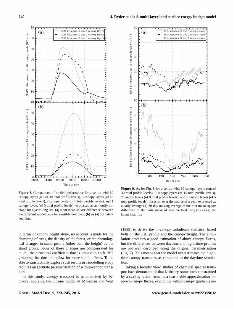
Tests were conducted for both hourly mean (Fig. 8) and

daily mean (Fig. 9), both calculated over the course of a year,

and for a moving average. These plots show the root mean

square (RMS) error between the original set-up and the mod-

ified number of levels. Figure 8 shows that there is already a

significant difference between the calculated hourly sensible

heat flux for the version of the model with 10 canopy layers

(30 total profile layers) and 5 canopy layers (15 total pro-

file layers), that reaches a peak of 28 W m−2, but that the

discrepancy is substantially larger for the 2 canopy layer (8

total levels) and a single canopy layer (5 total levels) cases.

In the case of the latent heat flux (Fig. 8b), the discrepancy

is most marked for the single canopy layer case, with a peak

difference of 60 W m−2. Considering the daily averages, for

sensible heat flux the difference between the different model

set-ups is always below 25 W m−2 (Fig. 9a) in all cases. For

latent heat flux, there is more considerable divergence, up to

42 W m−2, for the single canopy later set-up (Fig. 9b).

6 Discussion

The proposed model is able to simulate fluxes of sensible and

latent heat above the canopy over a long-term period, as has

been shown by simulation of conditions at a Fluxnet site on

a long-term, annual scale (Figs. 4 and 5), and over a con-

centrated, week-long period (Fig. 6). Although these figures

show a discrepancy between measured and modelled fluxes,

we see from Fig. 5 that the modelled overestimate of sensi-

ble heat flux is offset by an underestimation of latent heat flux

and of net radiation. In the study of land–atmosphere inter-

actions, the multi-layer model functions to a standard com-

parable to single-layer models, but calculates in more detail

in-canopy transport, the sources and sinks of heat, and pro-

files of temperature and specific humidity profiles. An earlier

iterative model applied to the same site (Haverd et al., 2009)

found differences of the order of 50 W m−2 at maximum for

the mean daily average latent and sensible above canopy heat

fluxes.



timestep (30 minutes)

0

200

400

600

Hab

ove

cano

py(W

/m

2) (a) T op of canopy mod.

T op of canopy meas.


0

200

400

600

Hat

2m(W

/m

2)

(b)


0

200

400

600

�E

abov

eca

nopy

(W/m

2) (c)


0

200

400

600

�E

at2m

(W/m

2)

(d)

6 7 8 9 10 11 12

D ate in November 2006 (tick denotes midnight local time)

�600

�400

�200

0

200

400

600

�F l

ux(m

eas.

-mod

.) (e) S ens. heat flux (difference meas. - mod.) L at. heat flux (difference meas. - mod.)

Figure 6. Short-term simulated and observed energy fluxes: (a) sensible heat fluxes at a height of 50 m; (b) as (a) for latent heat flux; (c)

measured and modelled sensible heat flux at 2 m above the ground; (d) modelled latent heat flux at 2 m above the ground (measurements not

available); (e) difference in measured and modelled sensible and latent heat flux at a height of 50 m.

The innovation of this model is the capacity to simulate

the behaviour of fluxes within the canopy, and the separa-

tion of the soil-level temperature from the temperature of

the vegetation levels. Uniquely for a canopy model, this is

achieved without iterations, as the mathematics has been de-

rived to use the same implicit coupling technique as the ex-

isting surface–atmosphere coupling applied in ORCHIDEE–

LMDz (Polcher et al., 1998; Best et al., 2004), but now over

the height of the canopy. This also means that the model is

scalable without impacting heavily on runtimes. For large-

scale applications, performance within the canopy must be

further constrained through comparison with intensive in-

canopy field campaigns from diverse ecosystems.

6.1 Simulation of aerodynamic resistance

In this study, the aerodynamic coefficient that is used in

single-layer models was replaced by an eddy diffusivity pro-



�3.5 �3.0 �2.5 �2.0 �1.5 �1.0 �0.5 0.0 0.50.0

0.2

0.4

0.6

0.8

1.0

1.2

1.4

Hei

ghta

bove

grou

nd

(z/h

) c

(a) Period 0h00 - 6h00

�0.5 0.0 0.5 1.0 1.5 2.0 2.5 3.0 3.5

(b)

Period 6h00 - 12h00

MeasuredtemperatureprofileModelledtemperatureprofile

�0.5 0.0 0.5 1.0 1.5 2.0 2.5 3.0 3.5� Temperature (K)

0.0

0.2

0.4

0.6

0.8

1.0

1.2

1.4

Hei

ghta

bove

grou

nd(z

/h ) c

(c) Period 12h00 - 18h00

�3.5 �3.0 �2.5 �2.0 �1.5 �1.0 �0.5 0.0 0.5� Temperature (K)

(d) Period 18h00 - 0h00

Figure 7. Vertical within-canopy temperature profiles for four 6 h periods corresponding to the same time period as in Fig. 6. Mean modelled

temperature profiles (blue) within the canopy against the measured temperature profiles (red) for the local time periods: (a) 00:00–06:00; (b)

06:00–12:00; (c) 12:00–18:00, and (d) 18:00–00:00 LT, both expressed as a difference from the temperature at the top of canopy.

file, the purpose of which is twofold: (i) to develop a transport

coefficient that is based on the vertical canopy profile, and

(ii) to more accurately represent the in-canopy gradients of

temperature and specific humidity. In this way, it was hoped

to contribute to a model that can better allow for such fea-

tures as vertical canopy gaps (i.e. trunk space between a well

separated under and overstorey), horizontal gaps, transport

and chemistry between different sections of the canopy, tree

growth and the mix of different kinds of vegetation in the

same surface layer simulation (e.g. Dolman, 1993). To be

able to do this, a height-based transport closure model was

used to simulate within-canopy transport.

The transport closure model used here can be compared

to the previous single-layer approach within ORCHIDEE.

In that approach, aerodynamic interaction between the land

surface and the atmosphere is parametrised by the atmo-

spheric resistance Ra and the architectural resistance R0. Ra

is typically calculated through consideration of the rough-

ness height of the canopy (i.e. small for flat surfaces, large

for uneven tall surfaces), which in turn is parametrised in sur-

face layer models by canopy height (e.g. LSCE/IPSL, 2012);

however, LAI can display a better correlation with roughness

length (a critical parameter) than it does to canopy height

(Beringer et al., 2005). In parametrising the roughness length



0

10

20

30

40

50

60

70RM

Sdi

ffere

nce

from

10ca

nopy

leve

ls(W

/m2 )

(a) Diff. between 10 and 5 canopy layersDiff. between 10 and 2 canopy layersDiff. between 10 and 1 canopy layers

00:00 04:00 08:00 12:00 16:00 20:00Time of day

0

10

20

30

40

50

60

70

RMS

diffe

renc

efr

om10

cano

pyle

vels

(W/m

2 )

(b)

Figure 8. Comparison of model performance for a set-up with 10

canopy layers (out of 30 total profile levels), 5 canopy layers (of 15

total profile levels), 2 canopy levels (of 8 total profile levels), and 1

canopy levels (of 5 total profile levels), expressed as an hourly av-

erage for a year-long run. (a) Root mean square difference between

the different model runs for sensible heat flux; (b) as (a) for latent

heat flux

in terms of canopy height alone, no account is made for the

clumping of trees, the density of the forest, or the phenolog-

ical changes in stand profile (other than the height) as the

stand grows. Some of these changes are compensated for

in R0, the structural coefficient that is unique to each PFT

grouping, but does not allow for more subtle effects. To be

able to satisfactorily explore such results in a modelling study

requires an accurate parametrisation of within-canopy trans-

port.

In this study, canopy transport is parametrised by K-

theory, applying the closure model of Massman and Weil

0

10

20

30

40

50

RMS

diffe

renc

efr

om10

cano

pyle

vels

(W/m

2 )

(a) Diff. between 10 and 5 canopy layersDiff. between 10 and 2 canopy layersDiff. between 10 and 1 canopy layers

0 60 120 180 240 300 360Day of year

0

10

20

30

40

50

RMS

diffe

renc

efr

om10

cano

pyle

vels

(W/m

2 )

(b)

Figure 9. As for Fig. 8 for a set-up with 10 canopy layers (out of

30 total profile levels), 5 canopy layers (of 15 total profile levels),

2 canopy levels (of 8 total profile levels), and 1 canopy levels (of 5

total profile levels), for a run over the course of a year, expressed as

a daily average (a) 20-day moving average of the root mean square

difference of the daily mean of sensible heat flux; (b) as (a) for

latent heat flux

(1999) to derive the in-canopy turbulence statistics, based

both on the LAI profile and the canopy height. The simu-

lation produces a good estimation of above-canopy fluxes,

but the differences between daytime and night-time profiles

are not well described using the original parametrisation

(Fig. 7). This means that the model overestimates the night-

time canopy transport, as compared to the daytime simula-

tion.

Taking a broader view, studies of chemical species trans-

port have demonstrated that K-theory, sometimes constrained

by a scaling factor, remains a reasonable approximation for

above-canopy fluxes, even if the within-canopy gradients are



not entirely correct (Gao et al., 1989; Dolman and Wallace,

1991; Makar et al., 1999; Wolfe and Thornton, 2011). The

justification for such a scaling factor seems to vary in terms

of the form of the canopy structure, likely related to canopy

openness (McNaughton and van den Hurk, 1995; Stroud

et al., 2005). Here, too, we find that a scaling factor is nec-

essary to match the gradient fluxes though the scaling factor

required varies according to the time of day. We now also

parametrise the effective phyto-element canopy drag coeffi-

cient, CDeff, in order to obtain a more accurate simulation.

For a completely satisfactory resolution of this issue, it will

be necessary to derive a method to reformulate the method

of Raupach (1989a, b) in an implicit form, which lies outside

the scope of this paper.

6.2 Simulation of energy partition throughout canopy

and soil surface

Trees in a spruce forest have been reported to account for 50–

60 % of the latent heat flux; moisture in the soil itself would

have a reduced impact due to soil shading (Baldocchi et al.,

2000). Another study found that the fraction of radiation that

reaches the soil ranges from 0.05 (forest) to 0.12 (tundra)

(Beringer et al., 2005). The same study found that the latent

heat flux correlates most closely with the leaf-level vapour

pressure deficit – that is to say the difference between the leaf

level saturation vapour pressure and the actual vapour pres-

sure of the outside air, rather than between air water vapour

pressure and the saturation vapour pressure at the soil level.

Since a single-layer canopy model regards both the canopy

and soil surface as the same entity, the aforementioned sub-

tleties will inevitably be lost in the modelling. Although, the

partition of energy between soil surface and vegetation is site

dependent – a well-hydrated site would behave differently to

one in an arid region – it is effects such as these that a more

realistic energy budget scheme should be able to simulate.

Being able to simulate separately the vegetation allows for

the partitioning of fluxes between the vegetation and the soil.

For example, from the measurements (Fig. 6a and b), we see

that approximately 50 % of the sensible heat that is measured

above the canopy is sourced not from the soil surface, but

from the overlying vegetation, as this is the difference be-

tween the measured flux at 1 m and that above the canopy.

The model simulated approximately 70 % of the sensible heat

being sourced from the soil. Hence, the model overestimates

the measured contribution from the soil. There is no equiva-

lent measurement at 1m for the latent heat flux, but the model

calculates that approximately 50 % of the latent heat flux is

sourced from the vegetation rather than the soil surface.

This model also simulates leaf temperature that may be

verified by leaf level measurements, where such measure-

ments exist (Helliker and Richter, 2008). Such a compari-

son would require additional developments (as is discussed

in the following section) because leaf temperature measure-

ments strongly depend on the approach that is used.

7 Outlook

This document lays out the framework for the model design,

but it allows for the further implementation of many features

in site-level to global-scale scenarios:

– As the method calculates leaf temperature and in-

canopy radiation, it will be possible to simulate the ex-

plicit emission by leaves of certain common biogenic

volatile organic compounds (BVOCs), such as isoprene

and monoterpene (Guenther et al., 1995, 2006). As the

method calculates in-canopy gradients of temperature,

specific humidity, and radiation, it is possible to sim-

ulate more accurately chemical reactions that depend

on these factors such as the NOx and O3 cycle within

and above canopies (Walton et al., 1997) and the forma-

tion and size distribution of aerosol interactions (Atkin-

son and Arey, 2003; Nemitz et al., 2004a, b; Ehn et al.,

2014), which may act as cloud condensation nuclei and

thus again feedback into radiation absorption interac-

tions at the atmospheric component of a coupled model

such as LMDz–ORCHIDEE.

– Separate computation of vegetation and soil tempera-

tures, which can be very different, and then estimate the

directional whole canopy temperature as measured by

remote sensing sensors. It may then be possible to as-

similate this variable from remote sensing products in

order to better constrain the energy budget.

– Recent research in ecology demonstrates further the

need to better understand canopy microclimates, and in

particular gradients of state variables such as temper-

ature and specific humidity, and radiation penetration.

For example, temperature gradients in the rainforest ex-

ert a key influence on the habitat choices of frogs, and

changes to such a microclimate threaten their survival

(Scheffers et al., 2013). In a similar vein, microclimate

affects in canopies can act as a buffer to changes in the

climate overall (i.e. the macro-climate) in terms of the

survival of species in the sub-canopy (Defraeye et al.,

2014). Therefore structural forest changes, such as for-

est thinning, will reduce buffer lag effect, but it is only

with well-designed canopy models that an informed

prediction of the long-term consequences of land man-

agement policies can be made.

8 Conclusions

A new numerical model for ORCHIDEE-CAN (revision

2966) has been developed that enables the simulation of

vertical canopy profiles of temperature and moisture us-

ing a non-iterative implicit scheme. This means that the

new model may also be used when coupled to an atmo-

spheric model, without compromising computer run-time.



Initial tests demonstrated that the model runs stably, balances

the energy budget at all levels, and provides a good simu-

lation of the measured field data, both on short timescales

of a few days, and over the course of a year. As demon-

strated, the model structure allows for coupling/linking to a

more physical-based albedo scheme (Pinty et al., 2006; Mc-

Grath et al., 2016; Naudts et al., 2015) and the implementa-

tion of a vertically discretised stomatal conductance scheme.

Reducing the vertical discretisation of the canopy from 10

layers to 5, 2, and 1 layer increased the root mean square er-

ror (RMSE) between the model and the observations for λE

and H and thus demonstrates the overall benefits of intro-

ducing a multi-layer energy budget scheme. The multi-layer

energy budget model component outlined here may be used

to simulate canopies in more detail and variety. It also offers

the potential to integrate with other parts of ORCHIDEE for

enhanced simulation of CO2 transport, emission of volatile

organic compounds (VOCs) and leaf-scale plant hydraulics.

The Supplement related to this article is available online

at doi:10.5194/gmd-9-223-2016-supplement.

Author contributions. J. Ryder and J. Polcher developed the nu-

merical scheme. Y. Chen and J. Ryder developed the parametrisa-

tion scheme. J. Ryder, J. Polcher, C. Ottlé, P. Peylin, and S. Luys-

saert designed the study, and J. Ryder and S. Luyssaert wrote

the manuscript with contributions from all co-authors. Y. Chen,

M. J. McGrath, J. Otto, K. Naudts, S. Luyssaert, and A. Valade

helped J. Ryder with integrating the multi-layer energy budget

model within ORCHIDEE-CAN. E. van Gorsel and V. Haverd pro-

vided field observations for the Tumbarumba site.

Acknowledgements. J. Ryder, Y. Chen, M. J. McGrath, J. Otto,

K. Naudts, and S. Luyssaert were funded through ERC starting

grant 242564 (DOFOCO), and A. Valade was funded through

ADEME (BiCaFF). ESA CCI Landcover also supported this

work. The study benefited from an STSM (COST, TERRABITES

ES0805) offered to J. Ryder. We thank the three anonymous review-

ers for their very helpful observations and suggestions. The authors

would like to thank A. Boone for sharing his numerical scheme

of an implicit coupling of snowpack and atmosphere tempera-

ture. Plots were produced using matplotlib software (Hunter, 2007).

Edited by: D. Lawrence

References

Atkinson, R. and Arey, J.: Gas-phase tropospheric chemistry of bio-

genic volatile organic compounds: a review, Atmos. Environ., 37,

197–219, doi:10.1016/S1352-2310(03)00391-1, 2003.

Baldocchi, D. D.: A multi-layer model for estimating sulfur dioxide

deposition to a deciduous oak forest canopy, Atmos. Environ.

(1967), 22, 869–884, doi:10.1016/0004-6981(88)90264-8, 1988.

Baldocchi, D. D. and Wilson, K.: Modeling CO2 and wa-

ter vapor exchange of a temperate broadleaved forest across

hourly to decadal time scales, Ecol. Model., 142, 155–184,

doi:10.1016/S0304-3800(01)00287-3, 2001.

Baldocchi, D. D., Law, B. E., and Anthoni, P. M.: On measuring and

modeling energy fluxes above the floor of a homogeneous and

heterogeneous conifer forest, Agr. Forest Meteorol., 102, 187–

206, doi:10.1016/S0168-1923(00)00098-8, 2000.

Baldocchi, D. D., Falge, E., Gu, L., Olson, R., Hollinger, D. Y.,

Running, S., Anthoni, P., Bernhofer, C., Davis, K., and Evans, R.:

FLUXNET: A new tool to study the temporal and spatial variabil-

ity of ecosystem-scale carbon dioxide, water vapor, and energy

flux densities., Bull. Am. Meteorol. Soc., 82, 2415–2434, 2001.

Ball, J. T., Woodrow, T., and Berry, J.: A model predicting stomatal

conductance and its contribution to the control of photosynthesis

under different environmental conditions, in: Proceedings of the

7th International Congress on Photosynthesis, 221–224, 1987.

Balsamo, G., Beljaars, A., Scipal, K., Viterbo, P., van den Hurk,

B., Hirschi, M., and Betts, A. K.: A revised hydrology for the

ECMWF model: verification from field site to terrestrial water

storage and impact in the integrated forecast system, J. Hydrom-

eteorol., 10, 623–643, doi:10.1175/2008JHM1068.1, 2009.

Beringer, J., Chapin, F. S., Thompson, C. C., and Mcguire, A. D.:

Surface energy exchanges along a tundra-forest transition and

feedbacks to climate, Agr. Forest Meteorol., 131, 143–161,

doi:10.1016/j.agrformet.2005.05.006, 2005.

Best, M. J., Beljaars, A. C. M., Polcher, J., and Viterbo, P.: A pro-

posed structure for coupling tiled surfaces with the planetary

boundary layer, J. Hydrometeorol., 5, 1271–1278, 2004.

Bonan, G. B.: Forests and climate change: forcings, feedbacks,

and the climate benefits of forests, Science, 320, 1444–1449,

doi:10.1126/science.1155121, 2008.

Bonan, G. B., Williams, M., Fisher, R. A., and Oleson, K. W.:

Modeling stomatal conductance in the earth system: linking

leaf water-use efficiency and water transport along the soil–

plant–atmosphere continuum, Geosci. Model Dev., 7, 2193–

2222, doi:10.5194/gmd-7-2193-2014, 2014.

Chen, Y., Ryder, J., Polcher, J., Peylin, P., Ottlé, C., Mcgrath, M.,

Naudts, K., Otto, J., Valade, A., Launiainen, S., Vesala, T., Black,

A., Ogee, J., Loustau, D., Moors, E., Longdoz, B., Foken, T.,

Knohl, A., Tiedemann, F., Aubinet, M., Heinesh, B., Juang, J.-

Y., van Gorsel, E., Haverd, V., and Luyssaert, S.: Calibration and

validation a new large scale multi-layer energy budget scheme in

ORCHIDEE-CAN, in preparation, 2016.

Defraeye, T., Derome, D., Verboven, P., Carmeliet, J., and Nico-

lai, B.: Cross-scale modelling of transpiration from stom-

ata via the leaf boundary layer, Ann. Botany, 114, 711–723,

doi:10.1093/aob/mct313, 2014.

de Noblet-Ducoudré, N., Boisier, J.-P., Pitman, A., Bonan, G. B.,

Brovkin, V., Cruz, F., Delire, C., Gayler, V., van den Hurk, B. J.

J. M., Lawrence, P. J., van der Molen, M. K., Müller, C., Reick,

C. H., Strengers, B. J., and Voldoire, A.: Determining robust im-


http://dx.doi.org/10.5194/gmd-9-223-2016-supplement

http://dx.doi.org/10.1016/S1352-2310(03)00391-1

http://dx.doi.org/10.1016/0004-6981(88)90264-8

http://dx.doi.org/10.1016/S0304-3800(01)00287-3

http://dx.doi.org/10.1016/S0168-1923(00)00098-8

http://dx.doi.org/10.1175/2008JHM1068.1

http://dx.doi.org/10.1016/j.agrformet.2005.05.006

http://dx.doi.org/10.1126/science.1155121

http://dx.doi.org/10.5194/gmd-7-2193-2014

http://dx.doi.org/10.1093/aob/mct313


pacts of land-use-induced land cover changes on surface climate

over North America and Eurasia: Results from the first set of LU-

CID experiments, J. Climate, 25, 3261–3281, doi:10.1175/JCLI-

D-11-00338.1, 2012.

Dolman, A. J.: A multiple-source land surface energy balance

model for use in general circulation models, Agr. Forest Mete-

orol., 65, 21–45, doi:10.1016/0168-1923(93)90036-H, 1993.

Dolman, A. J. and Wallace, J.: Lagrangian and K-theory approaches

in modelling evaporation from sparse canopies, Q. J. Roy. Mete-

orol. Soc., 117, 1325–1340, 1991.

Ehn, M., Thornton, J. A., Kleist, E., Sipilä, M., Junninen, H., Pulli-

nen, I., Springer, M., Rubach, F., Tillmann, R., Lee, B., Lopez-

Hilfiker, F., Andres, S., Acir, I.-H., Rissanen, M., Jokinen, T.,

Schobesberger, S., Kangasluoma, J., Kontkanen, J., Nieminen,

T., Kurtén, T., Nielsen, L. B., Jø rgensen, S., Kjaergaard, H. G.,

Canagaratna, M., Maso, M. D., Berndt, T., Petäjä, T., Wahner,

A., Kerminen, V.-M., Kulmala, M., Worsnop, D. R., Wildt, J.,

and Mentel, T. F.: A large source of low-volatility secondary or-

ganic aerosol, Nature, 506, 476–479, doi:10.1038/nature13032,

2014.

Gao, W., Shaw, R. H., and Paw, K. T.: Observation of organized

structure in turbulent flow within and above a forest canopy,

Bound.-Lay. Meteorol., 47, 349–377, 1989.

Grace, J. and Wilson, J.: The Boundary Layer over a Populus Leaf,

J. Experiment. Botany, 27, 231–241, doi:10.1093/jxb/27.2.231,

1976.

Gu, L.: Modeling biophysical exchanges and micro-meteorology

in soil-vegetation-atmosphere continuum – Results from a two-

story boreal aspen forest, PhD Thesis, University of Virginia,

Charlotsville, Virginia, 265 pp., 1988.

Gu, L., Shugart, H. H., Fuentes, J. D., Black, T. A., and Shewchuk,

S. R.: Micrometeorology, biophysical exchanges and NEE de-

composition in a two-storey boreal forest – development and

test of an integrated model, Agr. Forest Meteorol., 94, 123–148,

1999.

Guenther, A., Karl, T., Harley, P., Wiedinmyer, C., Palmer, P. I.,

and Geron, C.: Estimates of global terrestrial isoprene emissions

using MEGAN (Model of Emissions of Gases and Aerosols from

Nature), Atmos. Chem. Phys., 6, 3181–3210, doi:10.5194/acp-6-

3181-2006, 2006.

Guenther, A. B., Nicholas, C., Fall, R., Klinger, L., Mckay, W. A.,

and Scholes, B.: A global model of natural volatile organic com-

pound emissions, J. Geophys. Res., 100, 8873–8892, 1995.

Haverd, V., Leuning, R., Griffith, D., Gorsel, E., and Cuntz, M.: The

turbulent Lagrangian time scale in forest canopies constrained by

fluxes, concentrations and source distributions, Bound.-Lay. Me-

teorol., 130, 209–228, doi:10.1007/s10546-008-9344-4, 2009.

Helliker, B. R. and Richter, S. L.: Subtropical to boreal con-

vergence of tree-leaf temperatures, Nature, 454, 511–514,

doi:10.1038/nature07031, 2008.

Hourdin, F.: Etude et simulation numérique de la circulation

générale des atmosphères planétaires, PhD thesis, Laboratoire de

Météorologie Dynamique, 1992.

Hunter, J. D.: Matplotlib: A 2D graphics environment, Comput. Sci.

Eng., 9, 90–95, 2007.

Jiménez, C., Prigent, C., Mueller, B., Seneviratne, S. I., Mc-

Cabe, M. F., Wood, E. F., Rossow, W. B., Balsamo, G., Betts,

A. K., Dirmeyer, P. A., Fisher, J. B., Jung, M., Kanamitsu,

M., Reichle, R. H., Reichstein, M., Rodell, M., Sheffield, J.,

Tu, K., and Wang, K.: Global intercomparison of 12 land

surface heat flux estimates, J. Geophys. Res., 116, D02102,

doi:10.1029/2010JD014545, 2011.

Krinner, G., Viovy, N., de Noblet-Ducoudré, N., Ogee, J., Polcher,

J., Friedlingstein, P., Ciais, P., Sitch, S., and Prentice, I. C.:

A dynamic global vegetation model for studies of the coupled

atmosphere-biosphere system, Global Biogeochem. Cy., 19, 1–

33, doi:10.1029/2003GB002199, 2005.

Lovell, J., Haverd, V., Jupp, D., and Newnham, G.: The Canopy

Semi-analytic Pgap And Radiative Transfer (CanSPART) model:

Validation using ground based lidar, Agr. Forest Meteorol., 158–

159, 1–12, doi:10.1016/j.agrformet.2012.01.020, 2012.

LSCE/IPSL: ORCHIDEE documentation, available at: forge.ipsl.

jussieu.fr/orchidee/wiki/Documentation (last access: 16 Decem-

ber 2015), 2012.

Makar, P. A., Fuentes, J. D., Wang, D., Staebler, R. M., and Wiebe,

H. A.: Chemical processing of biogenic hydrocarbons within and

above a temperate deciduous forest, J. Geophys. Res., 104, 3581–

3603, doi:10.1029/1998JD100065, 1999.

Massman, W. J. and Weil, J. C.: An analytical one-dimensional

second-order closure model of turbulence statistics and the la-

grangian time scale within and above plant canopies of arbitrary

structure, Bound.-Lay. Meteorol., 91, 81–107, 1999.

McGrath, M. J., Pinty, B., Ryder, J., Otto, J., and Luyssaert, S.: A

multilevel canopy radiative transfer scheme based on a domain-

averaged structure factor, in preparation, 2016.

McNaughton, K. G. and van den Hurk, B. J. J. M.: A ’Lagrangian’

revision of the resistors in the two-layer model for calculating

the energy budget of a plant canopy, Bound.-Lay. Meteorol., 74,

261–288, 1995.

Medlyn, B. E., Duursma, R. A., Eamus, D., Ellsworth, D. S., Pren-

tice, I. C., Barton, C. V. M., Crous, K. Y., De Angelis, P., Free-

man, M., and Wingate, L.: Reconciling the optimal and empiri-

cal approaches to modelling stomatal conductance, Glob. Change

Biol., 17, 2134–2144, doi:10.1111/j.1365-2486.2010.02375.x,

2011.

Monteith, J. and Unsworth, M. H.: Principles of Environmental

Physics, Elsevier, ISBN 0125051034, 9780125051033, 2008.

Naudts, K., Ryder, J., McGrath, M. J., Otto, J., Chen, Y., Valade,

A., Bellasen, V., Berhongaray, G., Bönisch, G., Campioli, M.,

Ghattas, J., De Groote, T., Haverd, V., Kattge, J., MacBean,

N., Maignan, F., Merilä, P., Penuelas, J., Peylin, P., Pinty, B.,

Pretzsch, H., Schulze, E. D., Solyga, D., Vuichard, N., Yan, Y.,

and Luyssaert, S.: A vertically discretised canopy description for

ORCHIDEE (SVN r2290) and the modifications to the energy,

water and carbon fluxes, Geosci. Model Dev., 8, 2035–2065,

doi:10.5194/gmd-8-2035-2015, 2015.

Nemitz, E., Sutton, M. A., Wyers, G. P., and Jongejan, P. A. C.:

Gas-particle interactions above a Dutch heathland: I. Surface

exchange fluxes of NH3, SO2, HNO3 and HCl, Atmos. Chem.

Phys., 4, 989–1005, doi:10.5194/acp-4-989-2004, 2004a.

Nemitz, E., Sutton, M. A., Wyers, G. P., Otjes, R. P., Mennen, M.

G., van Putten, E. M., and Gallagher, M. W.: Gas-particle inter-

actions above a Dutch heathland: II. Concentrations and surface

exchange fluxes of atmospheric particles, Atmos. Chem. Phys.,

4, 1007–1024, doi:10.5194/acp-4-1007-2004, 2004b.

Nobel, P. S.: Physiochemical and environmental plant physiology,

Elsevier, 3rd Edn., 2005.


http://dx.doi.org/10.1175/JCLI-D-11-00338.1

http://dx.doi.org/10.1175/JCLI-D-11-00338.1

http://dx.doi.org/10.1016/0168-1923(93)90036-H

http://dx.doi.org/10.1038/nature13032

http://dx.doi.org/10.1093/jxb/27.2.231

http://dx.doi.org/10.5194/acp-6-3181-2006


http://dx.doi.org/10.1007/s10546-008-9344-4

http://dx.doi.org/10.1038/nature07031

http://dx.doi.org/10.1029/2010JD014545

http://dx.doi.org/10.1029/2003GB002199


forge.ipsl.jussieu.fr/orchidee/wiki/Documentation

forge.ipsl.jussieu.fr/orchidee/wiki/Documentation

http://dx.doi.org/10.1029/1998JD100065

http://dx.doi.org/10.1111/j.1365-2486.2010.02375.x

http://dx.doi.org/10.5194/gmd-8-2035-2015




Ogée, J., Brunet, Y., Loustau, D., Berbigier, P., and Delzon,

S.: MuSICA, a CO2, water and energy multilayer, multi-

leaf pine forest model: evaluation from hourly to yearly time

scales and sensitivity analysis, Glob. Change Biol., 9, 697–717,

doi:10.1046/j.1365-2486.2003.00628.x, 2003.

Ozflux: Description of Tumbarumba monitoring station, available

at: www.ozflux.org.au/monitoringsites/tumbarumba (last access:

16 December 2015), 2013.

Park, G.-H., Gao, X., and Sorooshian, S.: Estimation of surface

longwave radiation components from ground-based historical

net radiation and weather data, J. Geophys. Res., 113, D04207,

doi:10.1029/2007JD008903, 2008.

Penman, H. L. and Schofield, R. K.: Some physical aspects of as-

similation and transpiration, Symp. Soc. Exp. Biol., 5, 115–129,

1951.

Pinty, B., Lavergne, T., Dickinson, R. E., Widlowski, J.-L., Go-

bron, N., and Verstraete, M. M.: Simplifying the interac-

tion of land surfaces with radiation for relating remote sens-

ing products to climate models, J. Geophys. Res., 111, 1–20,

doi:10.1029/2005JD005952,

Pitman, A. J., de Noblet-Ducoudré, N., Cruz, F. T., Davin, E. L.,

Bonan, G. B., Brovkin, V., Claussen, M., Delire, C., Ganzeveld,

L., Gayler, V., van den Hurk, B. J. J. M., Lawrence, P. J.,

van der Molen, M. K., Müller, C., Reick, C. H., Seneviratne,

S. I., Strengers, B. J., and Voldoire, A.: Uncertainties in climate

responses to past land cover change: First results from the LU-

CID intercomparison study, Geophys. Res. Lett., 36, L14814,

doi:10.1029/2009GL039076, 2009.

Polcher, J., McAvaney, B., Viterbo, P., Gaertner, M., Hahmann, A.,

Mahfouf, J.-F., Noilhan, J., Phillips, T., Pitman, A. J., Schlosser,

C., Schulz, J.-P., Timbal, B., Verseghy, D. L., and Xue, Y.: A

proposal for a general interface between land surface schemes

and general circulation models, Global Planet. Change, 19, 261–

276, 1998.

Press, W. H.: Numerical recipes in Fortran 77, 2nd Edn., Cambridge

University Press, 1992.

Raupach, M. R.: Applying Lagrangian fluid mechanics to infer

scalar source distributions from concentration profiles in plant

canopies, Agr. Forest Meteorol., 47, 85–108, 1989a.

Raupach, M. R.: A practical Lagrangian method for relat-

ing scalar concentrations to source distributions in vegeta-

tion canopies, Quarterly J. Roy. Meteorol. Soc., 115, 609–632,

doi:10.1256/smsqj.48709, 1989b.

Richtmyer, R. D. and Morton, K. W.: Difference Methods for

Initial-Value Problems, 2nd Edn., Wiley-Interscience, 1967.

Saux-Picart, S., Ottlé, C., Perrier, A., Decharme, B., Coudert,

B., Zribi, M., Boulain, N., Cappelaere, B., and Ramier, D.:

SEtHyS_Savannah: A multiple source land surface model ap-

plied to Sahelian landscapes, Agr. Forest Meteorol., 149, 1421–

1432, doi:10.1016/j.agrformet.2009.03.013, 2009.

Scheffers, B. R., Phillips, B. L., Laurance, W. F., Sodhi, N. S., Dies-

mos, A., Williams, E., and Williams, S. E.: Increasing arboreality

with altitude: a novel biogeographic dimension, Proc. Roy. Soc.

B, 280, 1–9, doi:10.1098/rspb.2013.1581, 2013.

Schlosser, C. A. and Gao, X.: Assessing Evapotranspiration

Estimates from the Second Global Soil Wetness Project

(GSWP-2) Simulations, J. Hydrometeorol., 11, 880–897,

doi:10.1175/2010JHM1203.1, 2010.

Schulz, J.-P., Dümenil, L., and Polcher, J.: On the Land Surface–

Atmosphere Coupling and Its Impact in a Single-Column Atmo-

spheric Model, Journal of Applied Meteorology, 40, 642–663,

doi:10.1175/1520-0450(2001)040<0642:OTLSAC>2.0.CO;2,

2001.

Seneviratne, S. I., Corti, T., Davin, E. L., Hirschi, M.,

Jaeger, E. B., Lehner, I., Orlowsky, B., and Teuling,

A. J.: Investigating soil moisture–climate interactions in a

changing climate: A review, Earth-Sci. Rev., 99, 125–161,

doi:10.1016/j.earscirev.2010.02.004, 2010.

Shuttleworth, W. J. and Wallace, J. S.: Evaporation from sparse

crops – an energy combination theory, Q. J. Roy. Meteorol. Soc.,

111, 839–855, doi:10.1256/smsqj.46909, 1985.

Singles, R., Sutton, M., and Weston, K.: A multi-layer model

to describe the atmospheric transport and deposition of

ammonia in Great Britain, Atmos. Environ., 32, 393–399,

doi:10.1016/S1352-2310(97)83467-X, 1998.

Sinoquet, H., Le Roux, X., Adam, B., Ameglio, T., and Daudet,

F. A.: RATP: a model for simulating the spatial distribution

of radiation absorption, transpiration and photosynthesis within

canopies: application to an isolated tree crown, Plant Cell

Environ., 24, 395–406, doi:10.1046/j.1365-3040.2001.00694.x,

2001.

Stroud, C., Makar, P. A., Karl, T., Guenther, A. B., Geron, C.,

Turnipseed, A., Nemitz, E. G., Baker, B., Potosnak, M. J., and

Fuentes, J. D.: Role of canopy-scale photochemistry in modify-

ing biogenic-atmosphere exchange of reactive terpene species:

Results from the CELTIC field study, J. Geophys. Res., 110, 1–

14, doi:10.1029/2005JD005775, 2005.

Verhoef, A. and Allen, S. J.: A SVAT scheme describing en-

ergy and CO2 fluxes for multi-component vegetation: calibration

and test for a Sahelian savannah, Ecol. Model., 127, 245–267,

doi:10.1016/S0304-3800(99)00213-6, 2000.

Vieno, M.: The use of an atmospheric chemistry-transport model

(FRAME) over the UK and the development of its numerical and

physical schemes, PhD thesis, University of Edinburgh, 2006.

Vuichard, N. and Papale, D.: Filling the gaps in meteorological con-

tinuous data measured at FLUXNET sites with ERA-Interim re-

analysis, Earth Syst. Sci. Data, 7, 157–171, doi:10.5194/essd-7-

157-2015, 2015.

Waggoner, P. E., Furnival, G. M., and Reifsnyder, W. E.: Simulation

of the microclimate in a forest, Forest Sci., 15, 37–45, 1969.

Walton, S., Gallagher, M. W., and Duyzer, J. H.: Use of a de-

tailed model to study the exchange of NOx and O3 above and

below a deciduous canopy, Atmos. Environ., 31, 2915–2931,

doi:10.1016/S1352-2310(97)00126-X, 1997.

Wohlfahrt, G. and Cernusca, A.: Momentum transfer by a moun-

tain meadow canopy: a simulation analysis based on Massman’s

(1997) model, Bound.-Lay. Meteorol., 103, 391–407, 2002.

Wolfe, G. M. and Thornton, J. A.: The Chemistry of Atmosphere-

Forest Exchange (CAFE) Model – Part 1: Model descrip-

tion and characterization, Atmos. Chem. Phys., 11, 77–101,

doi:10.5194/acp-11-77-2011, 2011.

Yamazaki, T., Kondo, J., and Watanabe, T.: A heat-balance model

with a canopy of one or two layers and its application to field

experiments, J. Appl. Meteorol., 31, 86–103, 1992.


http://dx.doi.org/10.1046/j.1365-2486.2003.00628.x

www.ozflux.org.au/monitoringsites/tumbarumba

http://dx.doi.org/10.1029/2007JD008903

http://dx.doi.org/10.1029/2005JD005952

http://dx.doi.org/10.1029/2009GL039076

http://dx.doi.org/10.1256/smsqj.48709


http://dx.doi.org/10.1098/rspb.2013.1581

http://dx.doi.org/10.1175/2010JHM1203.1

http://dx.doi.org/10.1175/1520-0450(2001)040<0642:OTLSAC>2.0.CO;2

http://dx.doi.org/10.1016/j.earscirev.2010.02.004

http://dx.doi.org/10.1256/smsqj.46909

http://dx.doi.org/10.1016/S1352-2310(97)83467-X

http://dx.doi.org/10.1046/j.1365-3040.2001.00694.x

http://dx.doi.org/10.1029/2005JD005775

http://dx.doi.org/10.1016/S0304-3800(99)00213-6

http://dx.doi.org/10.5194/essd-7-157-2015

http://dx.doi.org/10.5194/essd-7-157-2015

http://dx.doi.org/10.1016/S1352-2310(97)00126-X



Zhao, W. and Qualls, R. J.: A multiple-layer canopy scatter-

ing model to simulate shortwave radiation distribution within

a homogeneous plant canopy, Water Resour. Res., 41, 1–16,

doi:10.1029/2005WR004016, 2005.

Zhao, W. and Qualls, R. J.: Modeling of long-wave and net ra-

diation energy distribution within a homogeneous plant canopy

via multiple scattering processes, Water Resour. Res., 42, 1–13,

doi:10.1029/2005WR004581, 2006.


http://dx.doi.org/10.1029/2005WR004016

http://dx.doi.org/10.1029/2005WR004581

Documents

A multi-layer land surface energy budget model for ...pubman.mpdl.mpg.de/pubman/item/escidoc:2538667:7/... · forced with the same micro-meteorological data (Jiménez et al.,2011)