A MULTI-LEVEL MIXED-EFFECTS MODEL FOR INDIVIDUAL

The Pennsylvania State University

The Graduate School

A MULTI-LEVEL MIXED-EFFECTS MODEL

FOR INDIVIDUAL PARTICIPANT DATA META-ANALYSIS

A Dissertation in

Biostatistics

by

Ying Zhang

Ó 2019 Ying Zhang

Submitted in Partial Fulfillment

of the Requirements

for the Degree of

Doctor of Philosophy

August 2019

The dissertation of Ying Zhang was reviewed and approved* by the following:

Vernon M. Chinchilli Distinguished Professor and Chair, Department of Public Health Sciences Professor of Statistics Dissertation Advisor Chair of Committee

Lan Kong Professor, Department of Public Health Sciences

David T. Mauger Professor, Department of Public Health Sciences

Christopher N. Sciamanna Professor and Vice Chair for Research Affairs, Department of Medicine Professor, Department of Public Health Sciences

Arthur Berg Associate Professor of Public Health Sciences Head of Biostatistics PhD Program

*Signatures are on file in the Graduate School

iii

ABSTRACT

Individual participant data (IPD) meta-analysis that combines and analyzes raw data from

multiple studies is considered to be more powerful and flexible compared with meta-analysis based

on summary statistics. A one-stage meta-analysis method based on IPD models all studies

simultaneously, accounting for the clustering of participants within each study. We propose a

statistical model that is a combination of a mixed-effect model and a multi-level model such that

the new model (1) contains fixed and random effects at each level, such as participant and study,

and (2) allows each study to have different lengths of follow-ups and different sets of covariates

for adjustment. The model is firstly developed for data with continuous outcomes, and then

extended to outcomes from an exponential family, such as binary, categorical, count outcomes, etc.

We conducted simulation studies to compare the proposed model with other meta-analysis methods

in 40 simulation scenarios with continuous and binary outcomes, respectively. We applied the

proposed model to three randomized studies from the National Heart, Lung, and Blood Institute to

evaluate the effect of reducing sodium intake on blood pressure control. The simulation studies

indicate the proposed model properly estimates the variability of data and maintains around 95%

coverage probability, while other meta-analytic methods tended to underestimate the variation and

suffered insufficient coverage probability when heterogeneity increases and sample size decreases.

The proposed one-stage model for IPD meta-analysis provides more flexibility than two-stage

methods and fixed-effects methods. It can properly account for the variability of the data and

provide reasonable pooled estimations, especially when a large amount of heterogeneity exists

across studies.

Keywords: meta-analysis; individual participant data; longitudinal data; mixed-effects model;

multi-level model; exponential family outcome

iv

TABLE OF CONTENTS

LIST OF FIGURES............................................................................................................. vi

LIST OF TABLES .............................................................................................................. vii

ACKNOWLEDGEMENTS ................................................................................................. viii

Chapter 1 Introduction........................................................................................................ 1

Chapter 2 Literature Review ............................................................................................... 3

2.1 Two-Stage IPD Meta-Analysis Methods ................................................................ 3 2.2 One-Stage IPD Meta-Analysis Methods ................................................................. 4 2.3 Methods for Different Outcomes and Longitudinal Data......................................... 4

Chapter 3 The One-Stage Multi-Level Mixed-Effects Model for IPD Meta-Analysis with Continuous Outcomes .................................................................................................. 6

3.1 Methods ................................................................................................................. 6 3.1.1 Model Introduction ...................................................................................... 6 3.1.2 Maximum Likelihood (ML) Estimation ....................................................... 9 3.1.3 Restricted Maximum Likelihood (REML) Estimation .................................. 16

3.2 Statistical Inference ................................................................................................ 22 3.2.1 Inference for Fixed Effects β ....................................................................... 22 3.2.2 Prediction of Random Effects γ#$ ................................................................. 25

3.3 Simulation Study ................................................................................................... 25 3.3.1 Simulation Design ....................................................................................... 25 3.3.2 Simulation Results ....................................................................................... 30 3.3.3 Supplemental Simulation Study ................................................................... 35

3.4 Real Data Application ............................................................................................ 37 3.4.1 Example Data - Blood Pressure Studies ....................................................... 37 3.4.1 Results ........................................................................................................ 39

Chapter 4 The One-Stage Multi-Level Mixed-Effects Model for IPD Meta-Analysis with Outcomes from An Exponential Family ....................................................................... 43

4.1 Methods ................................................................................................................. 43 4.1.1 Model Introduction ...................................................................................... 43 4.1.2 Quasi-likelihood Methods ............................................................................ 46 4.1.3 Laplace’s Method ........................................................................................ 52 4.1.3 Gaussian Quadrature.................................................................................... 55 4.1.4 Simulated Maximum Likelihood .................................................................. 58 4.1.4 Expectation-Maximization (EM) algorithm .................................................. 59

4.2 Inference for Fixed Effects β .................................................................................. 61 4.3 Simulation Study ................................................................................................... 62

4.3.1 Simulation Design ....................................................................................... 62

v

4.3.2 Simulation Results ....................................................................................... 66 4.4 Real Data Application ............................................................................................ 70

4.4.1 Example Data - Blood Pressure Studies ....................................................... 70 4.4.2 Results ........................................................................................................ 72

Chapter 5 Summary and Future Work................................................................................. 77

Appendix A Chapter 3 ........................................................................................................ 81

A.1 Simulation Study ................................................................................................... 81 A.2 Real Data Application ........................................................................................... 99

Appendix B Chapter 4 ........................................................................................................ 102

B.1 Simulation Study ................................................................................................... 102 B.2 Real Data Application ........................................................................................... 121

Bibliography ....................................................................................................................... 127

vi

LIST OF FIGURES

Figure 3-1: 3-level and 4-level Simulated Data Structure ..................................................... 26

Figure 3-2: Simulation results for the 3-level data structure with common covariates. .......... 31

Figure 3-3: Simulation results for the 3-level data structure with distinct covariates. ............ 32

Figure 3-4: Simulation results for the 4-level data structure with common covariates. .......... 34

Figure 3-5: Simulation results for the 4-level data structure with distinct covariates. ............ 34

Figure 3-6: Individual and pooled estimates with outcome, the change of SBP..................... 39

Figure 3-7: Meta-analysis methods comparison with outcomes, the change of SBP. ............. 40

Figure 3-8: Individual and pooled estimates with outcome, the change of DBP. ................... 41

Figure 3-9: Meta-analysis methods comparison with outcomes, the change of DBP. ............ 41

Figure 4-1: Simulation results for 3-level data structure with common covariates................. 67

Figure 4-2: Simulation results for 4-level data structure with common covariates................. 68

Figure 4-3: Simulation results for 3-level data structure with distinct covariates. .................. 69

Figure 4-4: Simulation results for 4-level data structure with distinct covariates. .................. 70

Figure 4-5: Individual estimates and pooled estimates with the binary SBP outcome............ 73

Figure 4-6: Meta-analysis methods comparison with the binary SBP outcome. .................... 73

Figure 4-7: Individual estimates and pooled estimates with the binary DBP outcome. .......... 74

Figure 4-8: Meta-analysis methods comparison with the binary DBP outcome. .................... 74

Figure 4-9: Individual estimates and pooled estimates with the ordinal SBP outcome. ......... 75

Figure 4-10: Meta-analysis methods comparison with the ordinal SBP outcome. ................. 76

Figure 4-11: Individual estimates and pooled estimates with the ordinal DBP outcome. ....... 76

Figure 4-12: Meta-analysis methods comparison with the ordinal DBP outcome. ................. 76

vii

LIST OF TABLES

Table 3-1: Sample size design in the simulation study with continuous outcomes. ............... 28

Table 3-2: Model specifications of the four test models. ...................................................... 30

Table 3-3: Model specifications of the supplemental simulation study. ................................ 35

Table 3-4: Results for the supplemental simulation study. .................................................... 36

Table 3-5: Study information summary of the NHLBI studies.............................................. 37

Table 3-6: Model fitting with NHLBI studies. ..................................................................... 38

Table 4-1: Sample size design in the simulation study with binary outcomes. ...................... 64

Table 4-2: Study information summary of the NHLBI studies.............................................. 71

Table 4-3: Model fitting with NHLBI studies. ..................................................................... 72

viii

ACKNOWLEDGEMENTS

I would like to sincerely express my appreciation to my dissertation advisor, Professor

Vernon M. Chinchilli, for his persistent support to my dissertation research in the past four years.

I am very grateful for his tremendous guidance, patience, inspiration, and knowledge. I would

also like to thank my committee members Professor Lan Kong, Professor David T. Mauger and

Professor Christopher N. Sciamanna for their valuable suggestions and comments all the way

through my dissertation research. I would like to thank the National Heart, Lung, and Blood

Institute for providing the data access to support this research work.

In addition, I would like to thank all the faculty members in the Department of Public

Health Sciences at The Pennsylvania State University for their support during my coursework and

dissertation research. I would like to thank my friends and classmates for their companionship

and encouragement. I would also like to thank my advisors during my master program education,

Dr. Xiaofei Wang at Duke University, and Dr. Herbert Pang at The University of Hong Kong.

Last but not the least, I would like to thank my parents for their unconditional love and

support all the time in my life.

Chapter 1

Introduction

Meta-analysis aims to combine and analyze multiple related studies to address a common

research question. Synthesizing information from related studies helps in improving the statistical

power in estimating parameters of interest, i.e., effect size, and thus helps researchers to reach more

accurate conclusions (Borenstein et al., 2011). Traditional meta-analysis usually aggregates study-

level summary statistics, such as the estimated effect size and its standard error, from publications

or study authors, and then estimates a weighted average value of these statistics based on a fixed-

effects model or a random-effects model. A fixed-effects model assumes all studies in the meta-

analysis share a common true effect, while a random-effects model assumes that the true effect of

each study is sampled from a distribution of these true effects, and thus a random-effects model

can accommodate between-study heterogeneity. With aggregate data, we are unable to investigate

the interaction effect between effect size and study-level covariates when estimating the weighted

average effect size, and we need to rely on another analysis technique, meta-regression, to explore

the modification effects of study-level covariates.

Individual participant data (IPD) meta-analysis, an alternative method to aggregate data

meta-analysis, was proposed and has become increasingly popular since 1990. Riley et al. (2010)

state that the application of IPD meta-analysis has increased very quickly, with an average of 49

applications per year after 2005. IPD contains the data recorded for each participant in a study,

which is a concept contrary to aggregate data. In an IPD meta-analysis, raw data from each study

are collected, synthesized and analyzed directly, preserving the clustering of participants within a

study. Many potential advantages of IPD meta-analysis over aggregate data meta-analysis have

been demonstrated (Riley et al., 2008; Riley et al., 2010). Firstly, IPD meta-analysis provides

2

higher statistical power with expanded sample size, and can avoid ecological bias and publication

bias caused by aggregate data meta-analysis. Aggregate data sometimes are poorly reported or

derived differently across studies, so the across-study relationships may differ from within-study

relationships. Also, aggregate data collected from published studies are likely to contain only

statistically significant results, which may result in publication bias. With IPD, these issues can be

avoided so that IPD meta-analysis can provide more consistent results. Secondly, more

sophisticated statistical methods for meta-analysis can be applied using IPD. Various approaches

have been developed for IPD meta-analysis, primarily including one-stage methods and two-stage

methods. Moreover, a modification effect of patient-level covariates on effect size can be modeled

and investigated simultaneously when estimating the synthesized effect size. Lastly, with raw data

from all studies, IPD meta-analysis guarantees consistent data checking and data cleaning across

studies, and provides more opportunities to address different research questions.

IPD meta-analysis has been shown to have several potential advantages over aggregate

meta-analysis, but corresponding methods for repeated measurements with modelling on source-

specific variances or for other types of outcomes are limited. Hierarchy is an inherent characteristic

of the meta-analysis data structure. For example, a meta-analysis usually involves multiple studies,

with participants within each study and sometimes multiple measurements within each participant.

Therefore, an optimal utilization of participant-level data should integrate information from each

hierarchical level, but it is often ignored in most meta-analysis research endeavors. In addition,

meta-analysis methods for longitudinal IPD for other outcome types are also of interest, such as

outcomes from an exponential family and time-to-event outcomes. All these issues stimulate the

motivation to develop statistical models for longitudinal IPD that can incorporate different types of

outcomes, and utilize the hierarchical feature of meta-analysis data.

3

Chapter 2

Literature Review

Most implementation methods for IPD meta-analysis can be categorized as two-stage or

one-stage methods. Both types of methods will be described in the next two sections. In addition,

the type of outcomes and the type of data may also vary in practice, and the methods that should

be adopted in different situations are different. The current methods for different type of

outcomes and longitudinal will be reviewed in section 2.3.

2.1 Two-Stage IPD Meta-Analysis Methods

There is a general model framework for the two-stage methods (Riley et al., 2015). Let 𝜃&'

be the effect size estimate for the 𝑘)* study, such that we can specify the general model as

𝜃&'~𝑁-𝜃', 𝑆'01

𝜃'~𝑁(𝜇, 𝜎0) (2.1)

where 𝜃&' follows a normal distribution with mean 𝜃' and variance 𝑆'0 for study 𝑘, and 𝜃' follows

another normal distribution with mean 𝜇 and variance 𝜎0 . 𝑆'0 represents within-study variance,

while 𝜎0 represents between-study variance. Model (1) is a random-effects model, and when 𝜎0 is

0, model (2.1) reduces to a fixed-effects model. Based on IPD, 𝜃&' and 𝑆6'0 for each study are

estimated in the first stage, and relevant covariates can be incorporated. The second stage is to

obtain an estimate of 𝜇 based on 𝜃&' and 𝑆6'0 through model (2.1).

4

2.2 One-Stage IPD Meta-Analysis Methods

For one-stage approaches, the IPD from all studies are modelled simultaneously,

accounting for the clustering of participants within each study. Consider 𝑦'8 as the continuous

outcome for the 𝑙)* participant within the 𝑘)* study. Then a general linear mixed-effects model

framework is specified as

𝑦'8 = 𝒙'8< 𝜷 + 𝒛'8< 𝜸'8 + 𝜀'8 (2.2)

where 𝒙'8 is a 𝑝 × 1 vector of the design effects for 𝜷, a 𝑝 × 1 vector of the parameters for fixed

effects, 𝒛'8 is a 𝑞 × 1 vector of the design effects for the random effects, 𝜸'8 is a 𝑞 × 1 vector of

the parameters for random effects, and 𝜀'8 is the random error term. The model is specified to

accommodate fixed effects and/or random effects, and any relevant covariates. Some parameters

in 𝜷 may be of study interest, such as the effect size parameter 𝜇 in model (2.1). The one-stage and

two-stage methods have been discussed further in Higgins et al. (2001), Riley et al. (2008), Mathew

et al. (2010), and Riley et al. (2015).

2.3 Methods for Different Outcomes and Longitudinal Data

Besides continuous outcomes, researchers sometimes are interested in treatment effects on

other outcomes, such as binary, ordinal, and time-to-event survival outcomes. For binary outcomes,

Turner et al. (2000) introduced a multi-level model framework to synthesize aggregate data and

IPD when IPD are not available in certain studies, and the authors discussed the differences of

inference methods in IPD and aggregate settings. For ordinal outcomes, Whitehead et al. (2001)

proposed a Bayesian proportional odds model framework. For a time-to-event outcome, there are

several articles that discussed and compared one-stage and two-stage methods, or fixed-effects and

5

random-effects models (Smith et al., 2005; Simmonds et al., 2013; Bowden et al., 2011; Simonds

et al., 2011; Rondeau et al., 2008).

In clinical studies, participants sometimes are followed for a period of time, and the

measurements of outcome on one participant may be collected at multiple time points. The data

with repeated measurements, or so-called longitudinal data, are common in clinical research

studies. The key to analyzing repeated measurement data is to appropriately incorporate the

correlation among repeated observations. With longitudinal IPD or aggregate data from multiple

studies, multivariate meta-analysis should be adopted. Jones et al. (2009) discussed the

implementation of multivariate meta-analysis based on longitudinal IPD. In the article, repeated

measurement time points were treated as a factor or as a continuous variable. For either approach

with a continuous outcome, one-stage or two-stage methods can be applied, and both types of

methods were compared. The specification of the covariance structure of the residual error allows

for the correlation between repeated observations on the same participant. However, the article

focuses on fixed-effects models, and models the variances altogether, which has the drawback of

being unable to distinguish the sources of variance. Another article from Trikalinos et al. (2012)

applied multivariate meta-analysis to aggregate data, using both fixed-effects and random-effects

models, treating time points as a factor.

Chapter 3

The One-Stage Multi-Level Mixed-Effects Model for IPD Meta-Analysis with Continuous Outcomes

This section will introduce the proposed model for IPD meta-analysis with continuous

outcomes, which adopts the features of a mixed-effects model and a multi-level model. The

proposed model can be applied to longitudinal or repeated measurement data, and will have the

capability to incorporate both fixed and random effects from each hierarchical level. Section 3.1

will introduce the model for continuous outcomes; section 3.2 will present the statistical inference

for fixed-effects and variance-covariance parameters; section 3.3 will describe the simulation study

conducted to evaluate the propose model; and section 3.4 will introduce the real data application

of the proposed model.

3.1 Methods

3.1.1 Model Introduction

For a continuous outcome variable, we propose a statistical model that is a combination of

a linear mixed-effects model (LMM) and a multi-level model that contains (a) fixed effects and

random effects for the longitudinal data from each participant within a study, and (b) fixed effects

and random effects for each study. The studies may be (a) observational studies or (b) randomized

interventional trials.

Let 𝑌'8(𝑡) denote the continuous outcome variable measured at time 𝑡 for the 𝑙)*

participant within the 𝑘)* study, 𝑘 = 1, 2, … , 𝐾 and 𝑙 = 1, 2, … , 𝑛' . Then

7

𝑌'8(𝑡) = 𝒙L,'8< (𝑡)𝜷L' + 𝒙M,'8< (𝑡)𝜷M + 𝒛'8< (𝑡)𝜸'8 + 𝜀'8(𝑡) + 𝒙'∗<𝜷∗

+ 𝒛'∗<𝜸'∗ + 𝜀'∗ (3.1)

where

• 𝒙L,'8(𝑡) is a participant-level, unique fixed-effects, 𝑟L' × 1vector of design effects and

covariates at time 𝑡for the 𝑙)* participant within the 𝑘)* study

• 𝜷L' is a participant-level, unique fixed-effects 𝑟L' × 1 vector of parameters for the 𝑘)*

study

• 𝒙M,'8(𝑡) is a participant-level, common fixed-effects, 𝑟M × 1vector of design effects and


• 𝜷M is a participant-level, common fixed-effects 𝑟M × 1 vector of parameters

• 𝒛'8(𝑡) is a participant-level, random-effects 𝑠' × 1vector of design effects and covariates

at time 𝑡 for the 𝑙)* participant within the 𝑘)* study

• 𝜸'8 is a participant-level, random-effects 𝑠' × 1 vector of parameters for the 𝑙)*

participant within the 𝑘)* study

• 𝜀'8(𝑡) is a participant-level, random error term at time 𝑡 for the 𝑙)* participant within the

𝑘)* study

• 𝒙'∗ is a study-level, fixed-effects, 𝑟∗ × 1vector of design effects and covariates for the 𝑘)*

study

• 𝜷∗ is a study-level, fixed-effects, 𝑟∗ × 1 vector of parameters

• 𝒛'∗ is a study-level, random-effects 𝑠∗ × 1vector of design effects and covariates for the

𝑘)* study

• 𝜸'∗ is a study-level, random-effects 𝑠∗ × 1 vector of parameters for the 𝑘)* study

• 𝜀'∗is a study-level, random error term for the 𝑘)* study

With respect to distributional assumptions,

8

• the 𝜸'8’s are independent with 𝜸'8~𝑁RS(𝟎, 𝚪'), where 𝚪' is a positive definite matrix

• 𝜺'8 = W𝜀'8(𝑡'8X)𝜀'8(𝑡'80) …𝜀'8-𝑡'8YZ[1\<~𝑁YZ[(𝟎, 𝚺'8),and the 𝜺'8 ’s are independent,

where 𝚺'8 is a positive definite matrix and a function of a parameter vector 𝝃

• the 𝜸'∗ ’s are independent with 𝜸'∗ ~𝑁_∗(𝟎, 𝚪∗), where 𝚪∗ is a positive definite matrix

• the 𝜀'∗’s are independent with 𝜀'∗~𝑁(0, 𝜎∗0)

• the 𝜸'8’s, the 𝜺'8’s, the 𝜸'∗ ’s, and the 𝜀'∗’s are mutually independent

We can rewrite model (3.1) for the 𝑙)* participant within the 𝑘)* study as

𝒀'8 = W𝑿L,'8 𝑿M,'8 𝟏YZ[×X𝒙'∗<\ d

𝜷L'𝜷M𝜷∗

e + W𝒁'8 𝟏YZ[×X𝒛'∗<\ g𝜸'8𝜸'∗h

+ (𝜺'8 + 𝟏YZ[×X𝜀'∗)

(3.2)

or

i𝑌'8(𝑡X)⋮

𝑌'8-𝑡YZ[1k

YZ[×X

= i𝒙L,'8< (𝑡X)

⋮𝒙L,'8< -𝑡YZ[1

𝒙M,'8< (𝑡X) 𝒙'∗<

⋮ ⋮𝒙M,'8< -𝑡YZ[1 𝒙'∗<

k

YZ[×(lmZnlonl∗)

d𝜷L'𝜷M𝜷∗

e(lmZnlonl∗)×X

+i𝒛'8< (𝑡X) 𝒛'∗<⋮ ⋮

𝒛'8< -𝑡YZ[1 𝒛'∗<k

YZ[×(_Zn_∗)

g𝜸'8𝜸'∗h(_Zn_∗)×X

+ i

𝜺'8(𝑡X) + 𝜀'∗⋮

𝜺'8-𝑡YZ[1 + 𝜀'∗k

YZ[×X

(3.3)

where 𝒀'8 = W𝑌'8(𝑡X)𝑌'8(𝑡0)…𝑌'8-𝑡YZ[1\<, 𝑿L,'8 = W𝒙L,'8< (𝑡X)𝒙L,'8< (𝑡0)…𝒙L,'8< -𝑡YZ[1\

<,

𝑿M,'8 = W𝒙M,'8< (𝑡X)𝒙M,'8< (𝑡0)…𝒙M,'8< -𝑡YZ[1\<, 𝒁'8 = W𝒛'8< (𝑡X)𝒛'8< (𝑡0)…𝒛'8< -𝑡YZ[1\

<, and 𝟏L×p is a

𝑢 × 𝑣 matrix of unit values.

The distributional assumptions lead to the following expressions for the expectation

vectors, the variance matrices, and the covariance matrices:

9

𝐸(𝒀'8) = W𝑿L,'8 𝑿M,'8 𝟏YZ[×X𝒙'∗<\ d

𝜷L'𝜷M𝜷∗

e (3.4)

𝑉𝑎𝑟(𝒀'8) = W𝒁'8 𝟏YZ[×X𝒛'∗<\ g

𝚪' 𝟎𝟎 𝚪∗

h v𝒁'8<

𝒛'∗ 𝟏X×YZ[w

+ -𝚺'8 + 𝜎∗0𝟏YZ[×YZ[1

= 𝒁'8𝚪'𝒁'8< + 𝚺'8 + (𝒛'∗<𝚪∗𝒛'∗ + 𝜎∗0)𝟏YZ[×YZ[ (3.5)

𝐶𝑜𝑣(𝒀'8, 𝒀'z) = 𝐶𝑜𝑣𝜸[𝐸(𝒀'8|𝜸), 𝐸(𝒀'z|𝜸)] + 𝐸𝜸[𝐶𝑜𝑣(𝒀'8|𝜸,𝒀'z|𝜸)]

= -𝒛'∗<𝚪∗𝒛'∗ 1𝟏YZ[×YZ~ + 𝜎∗0𝟏YZ[×YZ~

= (𝒛'∗<𝚪∗𝒛'∗ +𝜎∗0)𝟏YZ[×YZ~

(3.6)

𝐶𝑜𝑣(𝒀'8, 𝒀'�z) = 𝐶𝑜𝑣𝜸[𝐸(𝒀'8|𝜸), 𝐸(𝒀'�z|𝜸)]

+ 𝐸𝜸[𝐶𝑜𝑣(𝒀'8|𝜸,𝒀'�z|𝜸)] = 0 (3.7)

with 𝑘, 𝑘� = 1, 2, … , 𝐾, 𝑙 = 1, 2, … , 𝑛' and 𝑚 = 1, 2,… , 𝑛'�.

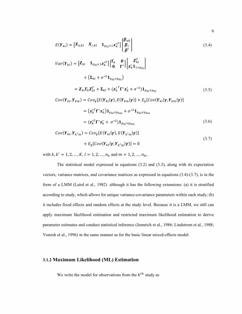
The statistical model expressed in equations (3.2) and (3.3), along with its expectation

vectors, variance matrices, and covariance matrices as expressed in equations (3.4)-(3.7), is in the

form of a LMM (Laird et al., 1982) although it has the following extensions: (a) it is stratified

according to study, which allows for unique variance-covariance parameters within each study; (b)

it includes fixed effects and random effects at the study level. Because it is a LMM, we still can

apply maximum likelihood estimation and restricted maximum likelihood estimation to derive

parameter estimates and conduct statistical inference (Jennrich et al., 1986; Lindstrom et al., 1988;

Vonesh et al., 1996) in the same manner as for the basic linear mixed-effects model.

3.1.2 Maximum Likelihood (ML) Estimation

We write the model for observations from the 𝑘)* study as

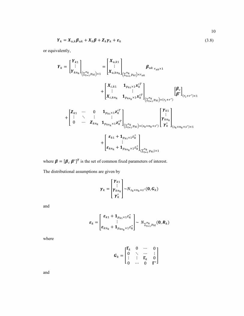
10

𝒀' = 𝑿L,'𝜷L' + 𝑿'𝜷 + 𝒁'𝜸' + 𝜺' (3.8)

or equivalently,

𝒀' = d𝒀'X⋮

𝒀'�Ze�∑ YZ[

�Z[�� ×X

= i𝑿L,'X⋮

𝑿L,'�Zk

�∑ YZ[�Z[�� ×lmZ

𝜷L'lmZ×X

+i𝑿M,'X 𝟏YZ�×X𝒙'

∗<

⋮ ⋮𝑿M,'�Z 𝟏YZ�Z×X𝒙'

∗<k

�∑ YZ[�Z[�� ×(lonl∗)

�𝜷M𝜷∗�(lonl∗)×X

+i𝒁'X ⋯ 0⋮ ⋱ ⋮0 ⋯ 𝒁'�Z

𝟏YZ�×X𝒛'

∗<

⋮𝟏YZ�Z×X𝒛'

∗<k

�∑ YZ[�Z[�� ×(_Z×�Zn_∗)

�

𝜸'X⋮

𝜸'�Z𝜸'∗

�

(_Z×�Zn_∗)×X

+i𝜺'X + 𝟏YZ�×X𝜀'

∗

⋮𝜺'�Z + 𝟏YZ�Z×X𝜀'

∗k

(∑ YZ[�Z[�� )×X

where 𝜷 = [𝜷M𝜷∗]𝑻 is the set of common fixed parameters of interest.

The distributional assumptions are given by

𝜸' = �

𝜸'X⋮

𝜸'�Z𝜸'∗

�~𝑁_Z×�Zn_∗(𝟎,𝑮')

and

𝜺' = i

𝜺'X + 𝟏YZ�×X𝜀'∗

⋮𝜺'�Z + 𝟏YZ�Z×X𝜀'

∗k~𝑁∑ YZ[

�Z[��

(𝟎, 𝑹')

where

𝑮' = i

𝚪' 0 ⋯0 ⋱ ⋯⋮0

⋮⋯

𝚪'0

0⋮0𝚪∗k

and

11

𝑹' = i

𝚺'X + 𝜎∗0𝟏YZ�×YZ� ⋯ 𝜎∗0𝟏YZ�×YZ�Z⋮ ⋱ ⋮

𝜎∗0𝟏YZ�Z×YZ� ⋯ 𝚺'�Z + 𝜎∗0𝟏YZ�Z×YZ�Z

k

Therefore, the covariance matrix of 𝒀' is

𝐶𝑜𝑣(𝒀') = 𝒁'𝑮'𝒁'< + 𝑹' = 𝚺'(𝝃)

The likelihood function 𝐿 for the data, 𝒀 = (𝒀X, 𝒀0, …, 𝒀�), is constructed as

𝐿(𝜷LX, … , 𝜷L�, 𝜷, 𝝃|𝒀) =� 𝑁(𝒀'; 𝑿L,'𝜷L' + 𝑿'𝜷, 𝚺'(𝝃))

�

'�X (3.9)

Here 𝜷 is a (𝑟M + 𝑟∗) × 1 vector of unknown regression parameters for common fixed effects

across 𝐾 studies and 𝝃 is a 𝑞 × 1 vector of unknown covariance parameters for random effects and

residual matrices. Taking the natural logarithm of 𝐿, the log-likelihood 𝑙 is

𝑙(𝜷LX, … , 𝜷L�, 𝜷, 𝝃|𝒀) = log �� 𝑁�𝒀'; 𝑿L,'𝜷L' + 𝑿'𝜷, 𝚺'(𝝃)�

�

'�X�

= 𝐶𝑜𝑛𝑠𝑡𝑎𝑛𝑡 −12� log|𝚺'|

�

'�X−12� -𝒀' − 𝑿L,'𝜷L' − 𝑿'𝜷1

<𝚺'�X(𝒀' − 𝑿L,'𝜷L' − 𝑿'𝜷)

�

'�X

The score vector 𝑺 is defined as

𝑺 =

⎣⎢⎢⎢⎡𝑺𝜷m�⋮

𝑺𝜷m£𝑺𝜷𝑺𝝃 ⎦

⎥⎥⎥⎤

=

⎣⎢⎢⎢⎢⎢⎢⎢⎢⎡𝜕𝑙𝜕𝜷LX⋮𝜕𝑙

𝜕𝜷L�𝜕𝑙𝜕𝜷𝜕𝑙𝜕𝝃 ⎦

⎥⎥⎥⎥⎥⎥⎥⎥⎤

where

𝑺𝜷mZ =

𝜕𝑙𝜕𝜷L'

= 𝑿L,'< 𝚺'�X-𝒀' − 𝑿L,'𝜷L' − 𝑿'𝜷1 = 𝑿L,'< 𝚺'�X𝒆'

𝑺𝜷 =

𝜕𝑙𝜕𝜷

=� 𝑿'<�

'�X𝚺'�X-𝒀' − 𝑿L,'𝜷L' − 𝑿'𝜷1 =� 𝑿'<

�

'�X𝚺'�X𝒆'

12

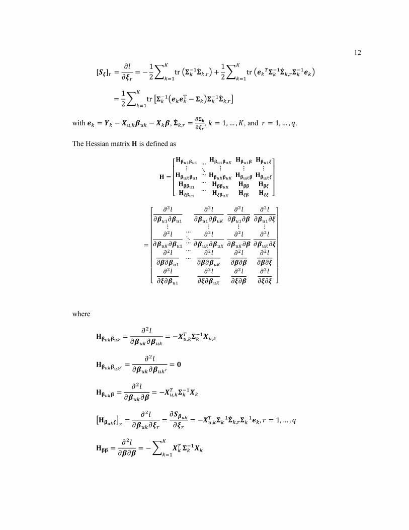
[𝑺𝝃]l =

𝜕𝑙𝜕𝝃l

= −12� tr-𝚺'�X�̇�',l1

�

'�X+12� tr-𝒆'<𝚺'�X�̇�',l𝚺'�X𝒆'1

�

'�X

=12� trW𝚺'�X-𝒆'𝒆'¬ − 𝚺'1𝚺'�X�̇�',l\

�

'�X

with 𝒆' = 𝒀' − 𝑿L,'𝜷L' − 𝑿'𝜷, �̇�',l =𝚺𝒌𝝃¯

, 𝑘 = 1,… , 𝐾, and 𝑟 = 1,… , 𝑞.

The Hessian matrix 𝐇 is defined as

𝐇 =

⎣⎢⎢⎢⎡𝐇𝛃m�𝛃m�

⋮𝐇𝛃m£𝛃m�𝐇𝛃𝛃m�𝐇𝝃𝛃m�

…⋱………

𝐇𝛃m�𝛃m£⋮

𝐇𝛃m£𝛃m£𝐇𝛃𝛃m£𝐇𝝃𝛃m£

𝐇𝛃m�𝛃⋮

𝐇𝛃m£𝛃𝐇𝛃𝛃𝐇𝝃𝛃

𝐇𝛃m�𝝃⋮

𝐇𝛃m£𝝃𝐇𝛃𝝃𝐇𝝃𝝃 ⎦

⎥⎥⎥⎤

=

⎣⎢⎢⎢⎢⎢⎢⎢⎢⎡ 𝜕0𝑙𝜕𝜷LX𝜕𝜷LX

⋮𝜕0𝑙

𝜕𝜷L�𝜕𝜷LX𝜕0𝑙

𝜕𝜷𝜕𝜷LX𝜕0𝑙

𝜕𝝃𝜕𝜷LX

…⋱………

𝜕0𝑙𝜕𝜷LX𝜕𝜷L�

⋮𝜕0𝑙

𝜕𝜷L�𝜕𝜷L�𝜕0𝑙

𝜕𝜷𝜕𝜷L�𝜕0𝑙

𝜕𝝃𝜕𝜷L�

𝜕0𝑙𝜕𝜷LX𝜕𝜷

⋮𝜕0𝑙

𝜕𝜷L�𝜕𝜷𝜕0𝑙𝜕𝜷𝜕𝜷𝜕0𝑙𝜕𝝃𝜕𝜷

𝜕0𝑙𝜕𝜷LX𝜕𝝃

⋮𝜕0𝑙

𝜕𝜷L�𝜕𝝃𝜕0𝑙𝜕𝜷𝜕𝝃𝜕0𝑙𝜕𝝃𝜕𝝃 ⎦

⎥⎥⎥⎥⎥⎥⎥⎥⎤

where

𝐇𝛃mZ𝛃mZ =

𝜕0𝑙𝜕𝜷L'𝜕𝜷L'

= −𝑿L,'< 𝚺'�X𝑿L,'

𝐇𝛃mZ𝛃mZ� =

𝜕0𝑙𝜕𝜷L'𝜕𝜷L'�

= 𝟎

𝐇𝛃mZ𝛃 =

𝜕0𝑙𝜕𝜷L'𝜕𝜷

= −𝑿L,'< 𝚺'�X𝑿'

W𝐇𝛃mZ𝝃\l =

𝜕0𝑙𝜕𝜷L'𝜕𝝃l

=𝜕𝑺𝜷mZ𝜕𝝃l

= −𝑿L,'< 𝚺'�X�̇�',l𝚺'�X𝒆', 𝑟 = 1,… , 𝑞

𝐇𝛃𝛃 =

𝜕0𝑙𝜕𝜷𝜕𝜷

= −� 𝑿'<�

'�X𝚺'�𝟏𝑿'

13

W𝐇𝛃𝝃\l =

𝜕0𝑙𝜕𝜷𝜕𝝃l

=𝜕𝑺𝜷𝜕𝝃l

= −� 𝑿'<�

'�X𝚺'�X�̇�',l𝚺'�X𝒆'

W𝐇𝝃𝝃\l_ = −12� trW– 𝚺'�X�̇�',l𝚺'�X�̇�',_ + 𝚺'�X�̈�',l_\

�

'�X

−12� trW−𝒆'<-−𝚺'�X-�̇�',l𝚺'�X�̇�',_ − �̈�',l_

�

'�X

+ �̇�',_𝚺'�X�̇�',l1𝚺'�X1𝒆'\

=12� trW𝚺'�X�̇�',l𝚺'�X�̇�',_ − 𝚺'�X�̈�',l_

�

'�X

− 𝚺'�X�̇�',l𝚺'�X�̇�',_𝚺'�X𝒆'𝒆'< + 𝚺'�X�̈�',l_𝚺'�X𝒆'𝒆'<

− 𝚺'�X�̇�',_𝚺'�X�̇�',l𝒆'𝒆'<\

=12� trW𝚺'�X-𝒆'𝒆'¬ − 𝚺'1𝚺'�X�̈�',l_\

�

'�X

−12� trW𝚺'�X�̇�',l𝚺'�X-2𝒆'𝒆'¬ − 𝚺'1𝚺'�X�̇�',_\

�

'�X

where �̈�',l_ =´𝚺𝒌𝝃¯𝝃µ

, 𝑘� = 1,… , 𝐾, 𝑘 ≠ 𝑘�, and 𝑟, 𝑠 = 1,… , 𝑞.

Solve 𝜷𝒖𝒌, 𝜷 and 𝝃 Using Newton-Raphson and Fisher Scoring Algorithms

The Newton-Raphson algorithm is an iterative procedure that computes new parameter

values �̧�L' , �̧�, and 𝝃¹ from current values 𝜷L' , 𝜷, and 𝝃 using

⎣⎢⎢⎡�̧�LX⋮�̧�𝝃¹ ⎦⎥⎥⎤= �

𝜷LX⋮𝜷𝝃

� − i𝐇𝛃m�𝛃m� ⋯ 𝐇𝛃m�𝝃

⋮ ⋱ ⋮𝐇𝝃𝛃m� ⋯ 𝐇𝝃𝝃

k

�X

⎣⎢⎢⎡𝑺𝜷m�⋮𝑺𝜷𝑺𝝃 ⎦

⎥⎥⎤

The Fisher scoring algorithm replaces the Hessian matrix by its expectation.

E-𝐇𝛃mZ𝛃mZ1 = 𝐇𝛃mZ𝛃mZ = −𝑿L,'< 𝚺'�X𝑿L,'

14

E(𝐇𝛃mZ𝛃mZ�) = 𝟎

E-𝐇𝛃mZ𝛃1 = 𝐇𝛃mZ𝛃 = −𝑿L,'< 𝚺'�X𝑿'

E(𝐇𝛃mZ𝝃) = 𝟎

E-𝐇𝛃𝛃1 = 𝐇𝛃𝛃 = −� 𝑿'<

�

'�X𝚺'�X𝑿'

E-𝐇𝝃𝛃1 = E-𝐇𝛃𝛏1 = 𝟎

E �W𝐇𝛏𝛏\𝒓𝒔� =X0∑ trW𝚺'�X(𝚺' − 𝚺')𝚺'�X�̈�',l_\�'�X −

X0∑ trW𝚺'�X�̇�',l𝚺'�X(2𝚺' − 𝚺')𝚺'�X�̇�',_\�'�X = − X

0∑ trW𝚺'�X�̇�',l𝚺'�X�̇�',_\�'�X

Because E(𝐇𝛃mZ𝝃) = 𝟎 and E-𝐇𝛃𝛏1 = 𝟎 , the updates of (�̧�L', �̧�) and 𝝃¹ based on the Fisher

scoring algorithm can be separated. The new values (�̧�L', �̧�) are obtained through:

i�̧�LX⋮�̧�k = d

𝜷LX⋮𝜷e − i

E(𝐇𝛃m�𝛃m�) ⋯ E(𝐇𝛃m�𝛃)⋮ ⋱ ⋮

E(𝐇𝛃𝛃m�) ⋯ E(𝐇𝛃𝛃)k

�X

d𝑺𝜷m�⋮𝑺𝜷

e (3.10)

The new values 𝝃¹ are then obtained through:

𝝃¹ = 𝝃 − E-𝐇𝛏𝛏1�𝟏𝑺𝝃(�̧�L', �̧�)

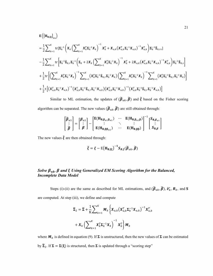
Solve 𝜷𝒖𝒌, 𝜷 and 𝝃 Using Generalized EM Scoring Algorithm for the Balanced, Incomplete Data Model

The generalized EM Scoring Algorithm is suitable for the balanced, but incomplete, data

model. If the variance-covariance matrix for a complete set of measurements on any study

participant is large and some participants display missing data in the balanced design, then this

algorithm has advantages over the Newton-Raphson and Fisher scoring methods.

The steps of this algorithm are as follows:

(i) (𝜷L', 𝜷) is updated via (�̧�L', �̧�) given in equation (3.10).

15

(ii) Let

𝒆'∗ = �𝒆'𝒆'n�~𝑁(𝟎,𝚺 = �𝚺'XX 𝚺'X0

𝚺'0X 𝚺'00�)

where 𝒆'∗ represents complete data for the 𝑘th study using sub-vectors 𝒆' = 𝒀' −

𝑿L,'𝜷L' − 𝑿'𝜷 as observed data and 𝒆'n as unobserved data. 𝚺 is partitioned

correspondingly.

Let 𝐸(𝒆'∗ |𝒆') = 𝒆¿'∗ , 𝐶𝑜𝑣(𝒆'∗ |𝒆') = 𝑷'. Then they can be calculated as

𝒆¿'∗ = �𝐸(𝒆')

𝐸(𝒆'n|𝒆')� = �

𝒆'𝚺'0X𝚺'XX�X 𝒆'

� = � 𝐈𝚺'0X𝚺'XX�X � 𝒆' = 𝑴'𝒆' (3.11)

𝑷' = �𝟎 𝟎𝟎 𝚺'00 − 𝚺'0X𝚺'XX�X 𝚺'X0

�

(iii) If 𝚺 is unstructured, then the new values �̧� are estimated as

�̧� =

1𝐾� (𝒆¿'∗ 𝒆¿'∗

< + 𝑷')�

'�X

If 𝚺 = 𝚺(𝛏) is structured, then 𝚺 is updated through a “scoring step”

𝛏¹ = 𝛏 − E-𝐇𝛏𝛏1�𝟏𝐬

where

[𝐬]l =12tr[𝚺�X-�̧� − 𝚺1𝚺�X�̇�l]

and

WE(𝐇𝛏𝛏)\l_ = −12tr[𝚺�X�̇�l𝚺�X�̇�_]

𝑟, 𝑠 = 1,… , 𝑞.

(iv) Let ℎ(𝝃) = − log|𝚺(𝝃)| − tr[𝚺�X(𝝃)�̧�]. To guarantee that the likelihood is increasing at

each step, check to see if ℎ-𝝃¹1 > ℎ(𝝃). If ℎ(𝝃) is not increased, then use partial stepping

to increase it (i.e., replace E-𝐇𝛏𝛏1�𝟏𝐬 by (E-𝐇𝛏𝛏1

�𝟏𝐬)/𝟐 until ℎ-𝝃¹1 > ℎ(𝝃)).

16

3.1.3 Restricted Maximum Likelihood (REML) Estimation

In ML estimation, the estimate of 𝝃 depends on the form of design matrices 𝑿L,' and 𝑿',

and incorrect specifications of 𝑿L,' and 𝑿' may result in an inconsistent estimate of 𝝃. Restricted

maximum likelihood (REML) estimation can be adopted to address this issue, which is based on

the likelihood function of transformed outcome data 𝒀∗. If we stack observations from all 𝐾 studies

together, we can have

d𝒀X⋮𝒀�e = i

𝑿L,X ⋯ 0⋮ ⋱ ⋮0 ⋯ 𝑿L,�

𝑿X⋮𝑿�k �

𝜷LX⋮

𝜷L�𝜷

� + d𝒁X ⋯ 0⋮ ⋱ ⋮0 ⋯ 𝒁�

e d𝜸X⋮𝜸�e + d

𝜺X⋮𝜺�e

or equivalently,

𝒀 = 𝑿𝜷È + 𝒁𝜸+ 𝜺

The transformed outcome data is constructed as 𝒀∗ = 𝑩<𝒀 such that the distribution of 𝒀∗

does not depend on the form of 𝑿. One choice of 𝑩 is based on the decomposition of ordinary least

square residuals, such that

𝑩𝑩< = 𝐈 − 𝑿(𝑿<𝑿)�X𝑿<

𝑩<𝑩 = 𝐈∗

cov-𝑩<𝒀, 𝜷Ì1 = 𝟎

where 𝑩 is a (∑ ∑ 𝑝'8�Z8�X

�'�X ) × 𝑞 matrix, 𝐈 is the (∑ ∑ 𝑝'8

�Z8�X

�'�X ) × (∑ ∑ 𝑝'8

�Z8�X

�'�X ) identity

matrix, 𝐈∗ is the 𝑞 × 𝑞 identity matrix, and 𝜷Ì = (𝜷ÍLX, … , 𝜷ÍL�, 𝜷Í) is the generalized least square

estimator of 𝜷È.

REML estimation leads to a consistent estimate of 𝝃 and it has the advantage that its

estimate of 𝝃 has less statistical bias than the ML estimate. The restricted log-likelihood function

𝑙Î is constructed as the log-likelihood function of 𝒀∗, and since

17

𝑙Î-𝜷ÍLX, … ,𝜷ÍL�,𝜷Í, 𝝃Ï𝒀1 = 𝑙(𝜷LX,… ,𝜷L�,𝜷, 𝝃|𝒀∗) ∝𝑙(𝜷LX,… , 𝜷L�,𝜷, 𝝃|𝒀)

𝑙-𝜷LX,… ,𝜷L�,𝜷, 𝝃Ï𝜷ÍLX,… , 𝜷ÍL�,𝜷Í1,

we can obtain

𝑙Î-𝜷ÍLX, … , 𝜷ÍL�, 𝜷Í, 𝝃Ï𝒀1

= 𝑙-𝜷ÍLX, … , 𝜷ÍL�, 𝜷Í, 𝝃|𝒀1 −12log Ñ� 𝑿'<𝚺'�X𝑿'

�

'�XÑ

−12� logÏ𝑿L,'< 𝚺'�X𝑿L,'Ï

�

'�X


�

'�X

−12� -𝒀' − 𝑿L,'𝜷ÍL'(𝝃) − 𝑿'𝜷Í(𝝃)1

<𝚺'�X(𝒀'

�

'�X

− 𝑿L,'𝜷ÍL'(𝝃) − 𝑿'𝜷Í(𝝃)) −12log Ñ� 𝑿'<𝚺'�X𝑿'

�

'�XÑ

−12� logÏ𝑿L,'< 𝚺'�X𝑿L,'Ï

�

'�X (3.12)

The REML estimates of 𝝃, 𝜷ÍL'(𝝃), and 𝜷Í(𝝃) may also be calculated by redefining 𝑙Î as a function

of 𝝃, 𝜷L' , and 𝜷. Therefore, the redefined 𝑙Î will be

𝑙Î(𝜷LX, … , 𝜷L�, 𝜷, 𝝃|𝒀)


�

'�X

−12� -𝒀' − 𝑿L,'𝜷L' − 𝑿'𝜷1

<𝚺'�X(𝒀' − 𝑿L,'𝜷L' − 𝑿'𝜷)

�

'�X

−12log Ñ� 𝑿'<𝚺'�X𝑿'

�

'�XÑ −

12� logÏ𝑿L,'< 𝚺'�X𝑿L,'Ï

�

'�X

The score vector 𝑺𝑹 is defined as

18

𝑺𝑹 =

⎣⎢⎢⎢⎡𝑺𝑹,𝜷m�⋮

𝑺𝑹,𝜷m£𝑺𝑹,𝜷𝑺𝑹,𝝃 ⎦

⎥⎥⎥⎤

=

⎣⎢⎢⎢⎢⎢⎢⎢⎢⎡𝜕𝑙Î𝜕𝜷LX⋮𝜕𝑙Î𝜕𝜷L�𝜕𝑙Î𝜕𝜷𝜕𝑙Î𝜕𝝃 ⎦

⎥⎥⎥⎥⎥⎥⎥⎥⎤

where

𝑺𝑹,𝜷mZ =

𝜕𝑙Î𝜕𝜷L'

= 𝑿L,'< 𝚺'�X-𝒀' − 𝑿L,'𝜷L' − 𝑿'𝜷1 = 𝑿L,'< 𝚺'�X𝒆' = 𝑺𝜷mZ

𝑺𝑹,𝜷 =

𝜕𝑙Î𝜕𝜷

=� 𝑿'<�

'�X𝚺'�X-𝒀' − 𝑿L,'𝜷L' − 𝑿'𝜷1 =� 𝑿'<

�

'�X𝚺'�X𝒆' = 𝑺𝜷

[𝑺𝑹,𝝃]l =

𝜕𝑙Î𝜕𝝃l

= −12� tr-𝚺'�X�̇�',l1

�

'�X+12� tr-𝒆'<𝚺'�X�̇�',l𝚺'�X𝒆'1

�

'�X

+12� 𝑡𝑟 vÒ� 𝑿'<𝜮'�X𝑿'

�

'�XÔ�X

𝑿'<𝜮'�X�̇�',l𝜮'�X𝑿'<w�

'�X

+12� 𝑡𝑟 g-𝑿L,'< 𝜮'�X𝑿L,'1

�X𝑿L,'< 𝜮'�X�̇�',l𝜮'�X𝑿L,'< h

�

'�X

=12� tr v𝚺'�X Õ𝒆'𝒆'¬ − 𝚺' + 𝑿' Ò� 𝑿'<𝚺'�X𝑿'

�

'�XÔ�X

𝑿'<�

'�X

+ 𝑿L,'-𝑿L,'< 𝜮'�X𝑿L,'1�X𝑿L,'< Ö 𝚺'�X�̇�',lw,

𝑟 = 1,… , 𝑞.

The Hessian matrix 𝐇𝐑 is defined as

𝐇𝐑 =

⎣⎢⎢⎢⎡𝐇𝐑,𝛃m�𝛃m�

⋮𝐇𝐑,𝛃m£𝛃m�𝐇𝐑,𝛃𝛃m�𝐇𝐑,𝝃𝛃m�

…⋱………

𝐇𝐑,𝛃m�𝛃m£⋮

𝐇𝐑,𝛃m£𝛃m£𝐇𝐑,𝛃𝛃m£𝐇𝐑,𝝃𝛃m£

𝐇𝐑,𝛃m�𝛃⋮

𝐇𝐑,𝛃m£𝛃𝐇𝐑,𝛃𝛃𝐇𝐑,𝝃𝛃

𝐇𝐑,𝛃m�𝝃⋮

𝐇𝐑,𝛃m£𝝃𝐇𝐑,𝛃𝝃𝐇𝐑,𝝃𝝃 ⎦

⎥⎥⎥⎤

where

19

𝐇𝐑,𝛃mZ𝛃mZ =

𝜕0𝑙Î𝜕𝜷L'𝜕𝜷L'

= −𝑿L,'< 𝚺'�X𝑿L,'

𝐇𝐑,𝛃mZ𝛃mZ� =

𝜕0𝑙Î𝜕𝜷L'𝜕𝜷L'�

= 𝟎

𝐇𝐑,𝛃mZ𝛃 =

𝜕0𝑙Î𝜕𝜷L'𝜕𝜷

= −𝑿L,'< 𝚺'�X𝑿'

W𝐇𝐑,𝛃mZ𝝃\l =

𝜕0𝑙𝜕𝜷L'𝜕𝝃l

=𝜕𝑺𝜷mZ𝜕𝝃l

= −𝑿L,'< 𝚺'�X�̇�',l𝚺'�X𝒆', 𝑟 = 1,… , 𝑞

𝐇𝐑,𝛃𝛃 =

𝜕0𝑙𝜕𝜷𝜕𝜷

= −� 𝑿'<�

'�X𝚺'�𝟏𝑿'

W𝐇𝐑,𝛃𝝃\l =

𝜕0𝑙𝜕𝜷𝜕𝝃l

=𝜕𝑺𝜷𝜕𝝃l

= −� 𝑿'<�

'�X𝚺'�X�̇�',l𝚺'�X𝒆'

W𝐇𝐑,𝝃𝝃\l_

= −12� trW−𝚺'�X�̇�',l𝚺'�X�̇�',_ + 𝚺'�X�̈�',l_\

�

'�X

−12� trW−𝒆'<-−𝚺'�X-�̇�',l𝚺'�X�̇�',_ − �̈�',l_ + �̇�',_𝚺'�X�̇�',l1𝚺'�X1𝒆'\

�

'�X

−12Ø−tr vÒ� 𝑿'<𝚺'�X𝑿'

�

'�XÔ�X

� -𝑿'<𝚺'�X�̇�',l𝚺'�X𝑿'1�

'�XÒ� 𝑿'<𝚺'�X𝑿'

�

'�XÔ�X

� -𝑿'<𝚺'�X�̇�',l𝚺'�X𝑿'1�

'�Xw

+ tr vÒ� 𝑿'<𝚺'�X𝑿'�

'�XÔ�X

� -𝑿'<𝚺'�X(�̇�',l𝚺'�X�̇�',_ − �̈�',l_ + �̇�',_𝚺'�X�̇�',l)𝚺'�X𝑿'1�

'�XwÙ

−12Ú−tr g-𝑿L,'< 𝚺'�X𝑿L,'1

�X-𝑿L,'< 𝚺'�X�̇�',l𝚺'�X𝑿L,'1-𝑿L,'< 𝚺'�X𝑿L,'1�X-𝑿L,'< 𝚺'�X�̇�',l𝚺'�X𝑿L,'1h

+ tr g-𝑿L,'< 𝚺'�X𝑿L,'1�X-𝑿L,'< 𝚺'�X(�̇�',l𝚺'�X�̇�',_ − �̈�',l_ + �̇�',_𝚺'�X�̇�',l)𝚺'�X𝑿L,'1hÛ

20

=12� tr[𝚺'�X Õ𝒆'𝒆'¬ − 𝚺' + 𝑿' Ò� 𝑿'<𝚺'�X𝑿'

�

'�XÔ�X

𝑿'< + 𝑿L,'-𝑿L,'< 𝚺'�X𝑿L,'1�X𝑿L,'< Ö𝚺'�X�̈�',l_]

�

'�X

−12� tr v𝚺'�X�̇�',l𝚺'�X Õ2𝒆'𝒆'¬ − 𝚺' + 2𝑿' Ò� 𝑿'<𝚺'�X𝑿'

�

'�XÔ�X

𝑿'<�

'�X

+ 2𝑿L,'-𝑿L,'< 𝚺'�X𝑿L,'1�X𝑿L,'< Ö𝚺'�X�̇�',_w

+12 tr

vÒ� 𝑿'<𝚺'�X𝑿'�

'�XÔ�X

� -𝑿'<𝚺'�X�̇�',l𝚺'�X𝑿'1�


�

'�XÔ�X

� -𝑿'<𝚺'�X�̇�',l𝚺'�X𝑿'1�

'�Xw

+12 tr

g-𝑿L,'< 𝚺'�X𝑿L,'1�X-𝑿L,'< 𝚺'�X�̇�',l𝚺'�X𝑿L,'1-𝑿L,'< 𝚺'�X𝑿L,'1

�X-𝑿L,'< 𝚺'�X�̇�',l𝚺'�X𝑿L,'1h,

𝑟, 𝑠 = 1,… , 𝑞

Solve 𝜷𝒖𝒌, 𝜷 and 𝝃 Using Newton-Raphson and Fisher Scoring Algorithms

Based on the Newton-Raphson algorithm, new parameter values �̧�L' , �̧� , and 𝝃¹ are

calculated as

⎣⎢⎢⎡�̧�LX⋮�̧�𝝃¹ ⎦⎥⎥⎤= �

𝜷LX⋮𝜷𝝃

� − i𝐇𝐑,𝛃m�𝛃m� ⋯ 𝐇𝐑,𝛃m�𝝃

⋮ ⋱ ⋮𝐇𝐑,𝝃𝛃m� ⋯ 𝐇𝐑,𝝃𝝃

k

�X

⎣⎢⎢⎡𝑺𝐑,𝜷m�⋮

𝑺𝐑,𝜷𝑺𝐑,𝝃 ⎦

⎥⎥⎤

The expectations of the elements of 𝐇𝐑 are

𝐄-𝐇𝐑,𝛃mZ𝛃mZ1 = 𝐇𝐑,𝛃mZ𝛃mZ = −𝑿L,'< 𝚺'�X𝑿L,'

𝐄(𝐇𝐑,𝛃mZ𝛃mZ� ) = 𝟎

𝐄-𝐇𝐑,𝛃mZ𝛃1 = 𝐇𝐑,𝛃mZ𝛃 = −𝑿L,'< 𝚺'�X𝑿'

𝐄(𝐇𝐑,𝛃mZ𝝃) = 𝟎

𝐄-𝐇𝐑,𝛃𝛃1 = 𝐇𝐑,𝛃𝛃 = −� 𝑿'<

�

'�X𝚺'�X𝑿'

𝐄-𝐇𝐑,𝝃𝛃1 = 𝐄-𝐇𝐑,𝛃𝛏1 = 𝟎

21

𝐄�W𝐇𝐑,𝛏𝛏\𝒓𝒔�

=12� tr[𝚺'�X Õ𝑿' Ò� 𝑿'<𝚺'�X𝑿'

�

'�XÔ�X

𝑿'< + 𝑿L,'-𝑿L,'< 𝚺'�X𝑿L,'1�X𝑿L,'< Ö𝚺'�X�̈�',l_]

�

'�X

−12� tr v𝚺'�X�̇�',l𝚺'�X Õ𝚺' + 2𝑿' Ò� 𝑿'<𝚺'�X𝑿'

�

'�XÔ�X

𝑿'< + 2𝑿L,'-𝑿L,'< 𝚺'�X𝑿L,'1�X𝑿L,'< Ö𝚺'�X�̇�',_w

�

'�X

+12 tr

vÒ� 𝑿'<𝚺'�X𝑿'�

'�XÔ�X

� -𝑿'<𝚺'�X�̇�',l𝚺'�X𝑿'1�


�

'�XÔ�X

� -𝑿'<𝚺'�X�̇�',l𝚺'�X𝑿'1�

'�Xw

+12 tg-𝑿L,'< 𝚺'�X𝑿L,'1

�X-𝑿L,'< 𝚺'�X�̇�',l𝚺'�X𝑿L,'1-𝑿L,'< 𝚺'�X𝑿L,'1�X-𝑿L,'< 𝚺'�X�̇�',l𝚺'�X𝑿L,'1h

Similar to ML estimation, the updates of (�̧�L', �̧�) and 𝝃¹ based on the Fisher scoring

algorithm can be separated. The new values (�̧�L', �̧�) are still obtained through:

i�̧�LX⋮�̧�k = d

𝜷LX⋮𝜷e − i

𝐄(𝐇𝐑,𝛃m�𝛃m�) ⋯ 𝐄(𝐇𝐑,𝛃m�𝛃)⋮ ⋱ ⋮

𝐄(𝐇𝐑,𝛃𝛃m�) ⋯ 𝐄(𝐇𝐑,𝛃𝛃)k

�X

d𝑺𝐑,𝜷m�⋮

𝑺𝐑,𝜷e

The new values 𝝃¹ are then obtained through:

𝝃¹ = 𝝃 − E-𝐇𝐑,𝛏𝛏1�𝟏𝑺𝑹,𝝃(�̧�L', �̧�)

Solve 𝜷𝒖𝒌, 𝜷 and 𝝃 Using Generalized EM Scoring Algorithm for the Balanced, Incomplete Data Model

Steps (i)-(ii) are the same as described for ML estimations, and (�̧�L', �̧�), 𝒆¿'∗ , 𝑹', and 𝐒

are computed. At step (iii), we define and compute

�̧�0 = �̧� +

1K� 𝑴' Ø𝑿L,'-𝑿L,'< 𝚺'�X𝑿L,'1

�X𝑿L,'<

�

'�X

+ 𝑿' Ò� 𝑿'<𝚺'�X𝑿'�

'�XÔ�X

𝑿'<Ù𝑴'

where 𝑴' is defined in equation (9). If 𝚺 is unstructured, then the new values of 𝚺 can be estimated

by �̧�0. If 𝚺 = 𝚺(𝛏) is structured, then 𝚺 is updated through a “scoring step”

22

𝛏¹ = 𝛏 − E-𝐇𝛏𝛏1�𝟏𝐬�

where

[𝐬�]l =12trW𝚺�X-�̧�0 − 𝚺1𝚺�X�̇�l\,

𝑟, 𝑠 = 1,… , 𝑞.

Let ℎ�(𝝃) = − log|𝚺(𝝃)| − tr[𝚺�X(𝝃)�̧�0] . ℎ�-𝝃¹1 > ℎ�(𝝃) is required to guarantee the

increase in the restricted likelihood. If ℎ�(𝝃) is not increasing, then use partial stepping to increase

it (i.e., replace 𝐄-𝐇𝛏𝛏1�𝟏𝐬� by (𝐄-𝐇𝛏𝛏1

�𝟏𝐬�)/𝟐 until ℎ�-𝝃¹1 > ℎ�(𝝃)).

3.2 Statistical Inference

3.2.1 Inference for Fixed Effects 𝜷

𝜷 is the set of common fixed parameters across all studies, which is usually of research

interest. For the inference of 𝜷, large sample tests can be performed with related confidence

intervals estimated, by using either the Wald chi-square test, adjusted Wald test, likelihood ratio

test, or score test. For a contrast matrix 𝑳à×(lonl∗), we want to test the null hypothesis 𝐻â: 𝑳𝜷 = 𝟎

versus 𝐻X: 𝑳𝜷 ≠ 𝟎.

1) Wald Chi-square Test

Based on the final estimate 𝜷Í , its estimated covariance matrix is

𝐶𝑜𝑣-𝜷Í1 = Ò� 𝑿'<

�

'�X𝚺Í'�𝟏𝑿'Ô

�X

23

where 𝚺Í' is the ML or the REML estimate of 𝚺' , and ∑ 𝑿'<�'�X 𝚺Í'�𝟏𝑿' is the empirical Fisher

information matrix. To test the null hypothesis, the Wald statistic is

𝐶0 = -𝑳𝜷Í1

<Ø𝑳Ò� 𝑿'<

�

'�X𝚺Í'�𝟏𝑿'Ô

�X

𝑳<Ù�X

-𝑳𝜷Í1,

and 𝐶0 is compared to percentiles from a 𝜒à0 distribution. If the number of rows of 𝑳, M, equals 1,

then an approximate (1 − 𝛼) × 100% confidence interval for 𝑳𝜷 is given by 𝑳𝜷Í ±

𝑧X�é/0ê𝑳𝐶𝑜𝑣-𝜷Í1𝑳<.

2) Adjusted Wald Test (Satterthwaite et al., 1941)

The Wald test relies on a large sample normal approximation to the sampling distribution

of 𝜷Í . When the sample size is not large enough, the Wald test statistic tends to be anti-conservative,

since additional variability is introduced through the estimate of 𝚺Í'. For a small sample, an adjusted

Wald statistic can be used, and it follows an F distribution. The adjusted Wald statistic is defined

as

𝐹 =

-𝑳𝜷Í1<Ú𝑳-∑ 𝑿'𝑻�

'�X 𝚺Í'�𝟏𝑿'1�X𝑳𝑻Û

�X-𝑳𝜷Í1

𝑟𝑎𝑛𝑘(𝑳)

which follows an approximate F distribution with numerator degrees of freedom as 𝑟𝑎𝑛𝑘(𝑳) and

denominator degrees of freedom estimated from the data. A typical choice for the denominator

degrees of freed is the total sample size minus (𝑟M + 𝑟∗), the dimension of 𝜷.

3) Likelihood Ratio Test

An alternative to the Wald test is the likelihood ratio test (LRT). Denote the maximized

ML log-likelihoods under null and alternative hypotheses as 𝑙6lìíLMìí(�̧�) and 𝑙6îL88(𝜷Í). The LRT

for two nested models can be constructed by comparing 𝑙6lìíLMìí(�̧�) and 𝑙6îL88(𝜷Í). The larger the

24

difference between 𝑙6lìíLMìí(�̧�) and 𝑙6îL88(𝜷Í), the stronger the evidence that the reduced model is

inadequate. The LRT statistic is

𝐺0 = −2(𝑙6lìíLMìí(�̧�) − 𝑙6îL88(𝜷Í))

and 𝐺0 is compared to percentiles from a 𝜒à0 distribution. If M, the number of rows of 𝑳, equals 1,

then an approximate (1 − 𝛼) × 100% confidence interval for 𝑳𝜷 can also be obtained by inverting

the LRT.

However, the REML log-likelihood cannot be used to compare nested models for 𝜷 ,

because the extra term in the REML log-likelihood depends on the model specification and the two

nested models for the mean are based on two entirely different sets of transformed responses.

4) Score Test

A score test is based on the null hypothesis, so the score function is obtained at 𝜷 = �̧�:

𝒖-�̧�1 =𝜕𝑙-𝜷, �̧�L', 𝛏¹Ï𝒀1

𝜕𝜷|𝜷��̧�

The information matrix 𝑰�̧� can be either the observed or expected information matrix evaluated at

𝜷 = �̧�.

𝑰�̧� = −´8�𝜷, 𝛏¹ñ𝒀�𝛃𝛃ò

|𝜷��̧� or 𝑰�̧� = 𝐸(−´8�𝜷, 𝛏¹ñ𝒀�𝛃𝛃ò

|𝜷��̧�)

The score test statistic is defined as

𝑠-�̧�1 = 𝒖-�̧�1<𝑰�̧��X𝒖-�̧�1

𝑠-�̧�1 is compared to percentiles from a 𝜒à0 distribution. If 𝑀 equals 1, then an approximate

(1 − 𝛼) × 100% confidence interval for 𝑳𝜷 can also be obtained by inverting the score test.

25

3.2.2 Prediction of Random Effects 𝜸ô𝒌

Consider the joint distribution of study-specific observations 𝒀' and random effects 𝜸'

within the 𝑘)* study, 𝑘 = 1,2, … , 𝐾.

�𝒀'𝜸'�~𝑁 Ò�𝑿L,'𝜷L' + 𝑿'𝜷

𝟎� , �𝚺'(𝝃) 𝒁'𝑮'𝑮'𝒁'< 𝑮'

�Ô (3.13)

where 𝑮'is defined in equation (3.8). Equation (3.13) implies that the conditional distribution of

𝜸'|𝒀' is

𝜸'|𝒀'~𝑁(𝑮'𝒁'<𝚺(𝝃)�X-𝒀' − 𝑿L,'𝜷L' − 𝑿'𝜷1, 𝚺'∗ (𝝃))

where

𝚺'∗ (𝝃) = 𝑮' − 𝑮'𝒁'<𝚺'(𝝃)�X𝒁'𝑮' = 𝑮' − 𝑮'𝒁'<-𝒁'𝑮'𝒁'< + 𝑹'1�X𝒁'𝑮'

Therefore, the empirical Bayes estimator for 𝜸'|𝒀' is given by

𝜸ô' = E[𝜸'|𝒀', 𝜷L', 𝜷, 𝝃] = 𝑮'𝒁'<𝚺'(𝝃)�X-𝒀' − 𝑿L,'𝜷L' − 𝑿'𝜷1

which also is called the best linear unbiased predictor (BLUP). 𝜷L', 𝜷, 𝝃 can be replaced by their

ML or REML estimates.

3.3 Simulation Study

3.3.1 Simulation Design

We conducted a simulation study to evaluate the proposed one-stage model for IPD meta-

analysis. The simulated data mimicked multi-center clinical trial data, with a two-arm, placebo-

controlled, parallel design, which evaluated the effect of an active treatment on reducing a patient’s

total cholesterol level.

26

We designed the simulated data to have a 3-level or a 4-level structure (Figure 3-1). For

the 3-level data, we assume the clinical data were collected from multiple studies, and each study

had different numbers of centers (study sites), and each center had different numbers of

participants. For the 4-level data, we assumed each participant within a center had different

numbers of visits, which was the visit level and resulted in longitudinal data. For both 3-level and

4-level multi-center data, we simulated several participant-level variables, including treatment

assignment (TRT; placebo or active treatment), baseline cholesterol level (base_cho; mg/dL), age

at enrollment, gender (male or female), race (Caucasian (Cau), African American (AA), Hispanic

(His) and other), diabetes disease status (yes or no), and cardiovascular disease status (CVD; yes

or no). Both base_cho and age were centered by their population means, respectively. We also

generated three study-level covariates to reflect the characteristics of each study, including the

mean of cohort sizes of centers within each study (𝑆𝑆zìõ�), the standard deviation of cohort sizes

of centers within each study (𝑆𝑆_)í ), and the chronological order of each study (order). We

generated two sets of study-level random effects, including study-level random intercept (rstudy) and

random effect for treatment effects across studies (rstudy_treatment). We imposed another two sets of

Figure 3-1: 3-level and 4-level Simulated Data Structure

27

random effects to the center level, including center-level random intercept (rcenter) and random effect

for baseline cholesterol level (rcenter_bc). With the 4-level data structure, we generated each

participant’s weight (lbs) as a repeated measurement variable, and each participant might have 3 to

5 visits. Weight was centered by its population mean before it was used. We removed the random

effect rcenter_bc and included an additional set of random intercepts for participant level (rparticipant).

The study-level treatment random effect (rstudy_treatment) is replaced by the study-level random effect

for treatment×visit (rstudy_treatment*visit).The primary parameter of interest is the difference of effect

between treatment groups in the 3-level data structure, and the parameter of interest is the difference

in slopes between treatment groups in the 4-level data structure.

Based on 3-level data, the mean function conditional on random effects used to generate

the outcome is

𝐸-𝑌'M8|𝑟_)Líö, 𝑟_)Líö_)lìõ)zì�), 𝑟Mì�)ìl, 𝑟Mì�)ìl_øM1

= 220 − 8 × 𝑇𝑅𝑇 + 0.2 × 𝑏𝑎𝑠𝑒_𝑐ℎ𝑜 + 0.2 × 𝑎𝑔𝑒

− 4 × 𝑔𝑒𝑛𝑑𝑒𝑟 + 4× 𝑟𝑎𝑐𝑒$$ + 6 × 𝑟𝑎𝑐𝑒&'_

− 0.8 × 𝑟𝑎𝑐𝑒()*ìl + 6 × 𝑑𝑖𝑎𝑏𝑒𝑡𝑒𝑠 + 6 × 𝐶𝑉𝐷

− 0.3 × 𝑆𝑆zìõ� + 1.5× 𝑆𝑆_)í − 0.5 × 𝑜𝑟𝑑𝑒𝑟 + 𝑟_)Líö

+ 𝑟_)Líö_)lìõ)zì�) × 𝑇𝑅𝑇 +𝑟Mì�)ìl

+ 𝑟Mì�)ìl_øM × 𝑏𝑎𝑠𝑒_𝑐ℎ𝑜

(3.14)

where 𝑌'M8 is the outcome for the 𝑙th participant from the 𝑐th center in the 𝑘th study.

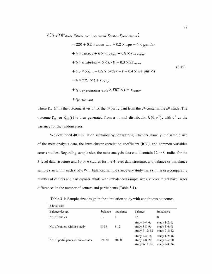
Based on 4-level data, the mean function conditional on random effects used to generate

the outcome is

28

𝐸-𝑌'M8(𝑡)|𝑟_)Líö, 𝑟_)Líö_)lìõ)zì�)∗p'_'), 𝑟Mì�)ìl, 𝑟Yõl)'M'Yõ�)1

= 220 + 0.2 × 𝑏𝑎𝑠𝑒_𝑐ℎ𝑜 + 0.2 × 𝑎𝑔𝑒 − 4× 𝑔𝑒𝑛𝑑𝑒𝑟

+ 4 × 𝑟𝑎𝑐𝑒$$ + 6× 𝑟𝑎𝑐𝑒&'_ − 0.8 × 𝑟𝑎𝑐𝑒()*ìl

+ 6 × 𝑑𝑖𝑎𝑏𝑒𝑡𝑒𝑠 + 6× 𝐶𝑉𝐷 − 0.3 × 𝑆𝑆zìõ�

+ 1.5 × 𝑆𝑆_)í − 0.5× 𝑜𝑟𝑑𝑒𝑟 − 𝑡 + 0.4×𝑤𝑒𝑖𝑔ℎ𝑡 × 𝑡

− 4 × 𝑇𝑅𝑇 × 𝑡 + 𝑟_)Líö

+ 𝑟_)Líö_)lìõ)zì�)∗p'_') × 𝑇𝑅𝑇 × 𝑡 +𝑟Mì�)ìl

+ 𝑟Yõl)'M'Yõ�)

(3.15)

where 𝑌'M8(𝑡) is the outcome at visit t for the 𝑙th participant from the 𝑐th center in the 𝑘th study. The

outcome 𝑌'M8 or 𝑌'M8(𝑡) is then generated from a normal distribution 𝑁(0, 𝜎0), with 𝜎0 as the

variance for the random error.

We developed 40 simulation scenarios by considering 3 factors, namely, the sample size

of the meta-analysis data, the intra-cluster correlation coefficient (ICC), and common variables

across studies. Regarding sample size, the meta-analysis data could contain 12 or 8 studies for the

3-level data structure and 10 or 6 studies for the 4-level data structure, and balance or imbalance

sample size within each study. With balanced sample size, every study has a similar or a comparable

number of centers and participants, while with imbalanced sample sizes, studies might have larger

differences in the number of centers and participants (Table 3-1).

Table 3-1: Sample size design in the simulation study with continuous outcomes.

3-level data

Balance design balance imbalance balance imbalance

No. of studies 12 8 12 8

No. of centers within a study 8-16 8-12 study 1-4: 6; study 5-8: 9; study 9-12: 12

study 1-2: 6; study 3-6: 9; study 7-8: 12

No. of participants within a center 24-70 20-30 study 1-4: 16; study 5-8: 20; study 9-12: 26


29

The ICC is usually defined as the between-study variance 𝜎øì).ìì�0 divided by the sum of

the between-study variance and the within-study variance (𝜎øì).ìì�0 + 𝜎.')*'�0 ) (Donner, 1986). As

the value of the ICC may be associated with the participant’s characteristics, we specified the ICC

values for the reference group, and altered the ICC as 0.1, 0.2, 0.3, 0.4, and 0.5. The reference

group is referred to subjects who are Caucasian males assigned to the control treatment group,

without diabetes or CVD and with mean base_cho and age. For example, suppose with 3-level data,

we have two subjects in the reference group from the same center of a study, then the ICC is equal

to

𝐼𝐶𝐶 =

𝜎l__)Líö0 + 𝜎l_Mì�)ìl0

𝜎l__)Líö0 + 𝜎l_Mì�)ìl0 + 𝜎0

where 𝑟_)Líö~𝑁(0, 𝜎l__)Líö0 ), 𝑟Mì�)ìl~𝑁(0, 𝜎l_Mì�)ìl0 ). We specified 𝜎0 as 225 in the simulation

study and 𝜎l__)Líö0 : 𝜎l_Mì�)ìl0 = 1: 2. As ICC ranged from 0.1, 0.2 to 0.5, we could decide the values

of 𝜎l__)Líö0 and 𝜎l_Mì�)ìl0 . More details about value specification could be found in the appendix A.

The covariates collected from each study could be the same or different. We considered

either common covariates from each study, or with distinct/unique variables. In scenarios with

distinct/unique variables, we chose gender, race, CVD, and diabetes information as study-specific

variables. In particular, gender was only available in study no. 3 and 5, race was available in study

4-level data







No. of visits of a participant 3-5

30

1, diabetes was available in study 7, and CVD was available in study 8. We examined each scenario

in 1000 simulation runs.

With each simulated dataset, we applied 4 test models to the data. The models were a two-

stage fixed-effects model, a two-stage random-effects model, a one-stage fixed-effects model, and

a one-stage model (our proposed model). Both two-stage methods still include center-level and

participant-level random effects in the first stage estimates, while the one-stage fixed-effects model

ignores all random effects, and the one-stage proposed model captures all random effects (Table 3-

2). To assess the performance of the 4 test models, we compare the average of mean estimates,

average of standard errors from simulation, and the coverage probability of containing the true

treatment effect among 1000 simulations.

3.3.2 Simulation Results

The average of mean estimates, the average of standard errors from each estimate, and the

coverage probability from 1000 simulations for the scenarios with common and distinct/unique

Table 3-2: Model specifications of the four test models. Test model Model fitting

two-stage fixed-effects 1st stage: study-level covariates, participant-level covariates, visit-level covariates*,

rcenter, rcenter_bc∆, rparticipant*; 2nd stage: a fixed-effects model to pool treatment effect

two-stage random-effects 1st stage: study-level covariates, participant-level covariates, visit-level covariates*,

rcenter, rcenter_bc∆, rparticipant*; 2nd stage: a random-effects model to pool treatment effect

one-stage fixed-effects participant-level covariates, visit-level covariates*

one-stage proposed study-level covariates, participant-level covariates, visit-level covariates*, rstudy,

rstudy_treatment, rcenter, rcenter_bc∆, rparticipant*

*: only used in 4-level data; ∆: only used in 3-level data

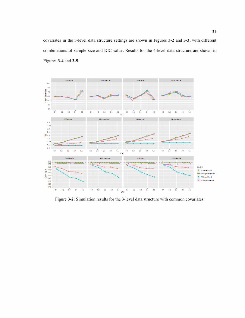
31

covariates in the 3-level data structure settings are shown in Figures 3-2 and 3-3, with different

combinations of sample size and ICC value. Results for the 4-level data structure are shown in

Figures 3-4 and 3-5.

Figure 3-2: Simulation results for the 3-level data structure with common covariates.

32

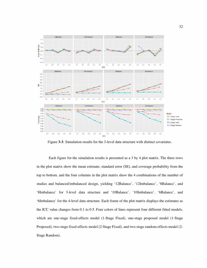
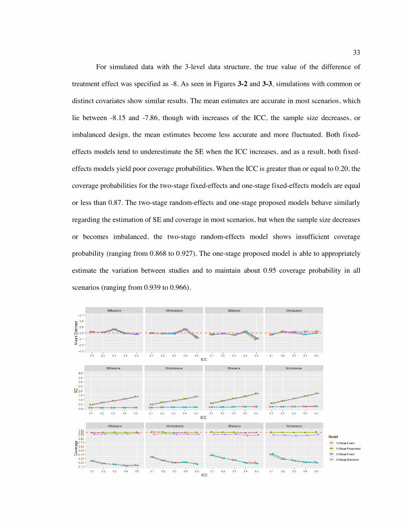
Each figure for the simulation results is presented as a 3 by 4 plot matrix. The three rows

in the plot matrix show the mean estimate, standard error (SE), and coverage probability from the

top to bottom, and the four columns in the plot matrix show the 4 combinations of the number of

studies and balanced/imbalanced design, yielding ‘12Balance’, ‘12Imbalance’, ‘8Balance’, and

‘8Imbalance’ for 3-level data structure and ‘10Balance’, ‘10Imbalance’, ‘6Balance’, and

‘6Imbalance’ for the 4-level data structure. Each frame of the plot matrix displays the estimates as

the ICC value changes from 0.1 to 0.5. Four colors of lines represent four different fitted models,

which are one-stage fixed-effects model (1-Stage Fixed), one-stage proposed model (1-Stage

Proposed), two-stage fixed-effects model (2-Stage Fixed), and two-stage random-effects model (2-

Stage Random).

Figure 3-3: Simulation results for the 3-level data structure with distinct covariates.

33

For simulated data with the 3-level data structure, the true value of the difference of

treatment effect was specified as -8. As seen in Figures 3-2 and 3-3, simulations with common or

distinct covariates show similar results. The mean estimates are accurate in most scenarios, which

lie between -8.15 and -7.86, though with increases of the ICC, the sample size decreases, or

imbalanced design, the mean estimates become less accurate and more fluctuated. Both fixed-

effects models tend to underestimate the SE when the ICC increases, and as a result, both fixed-

effects models yield poor coverage probabilities. When the ICC is greater than or equal to 0.20, the

coverage probabilities for the two-stage fixed-effects and one-stage fixed-effects models are equal

or less than 0.87. The two-stage random-effects and one-stage proposed models behave similarly

regarding the estimation of SE and coverage in most scenarios, but when the sample size decreases

or becomes imbalanced, the two-stage random-effects model shows insufficient coverage

probability (ranging from 0.868 to 0.927). The one-stage proposed model is able to appropriately

estimate the variation between studies and to maintain about 0.95 coverage probability in all

scenarios (ranging from 0.939 to 0.966).

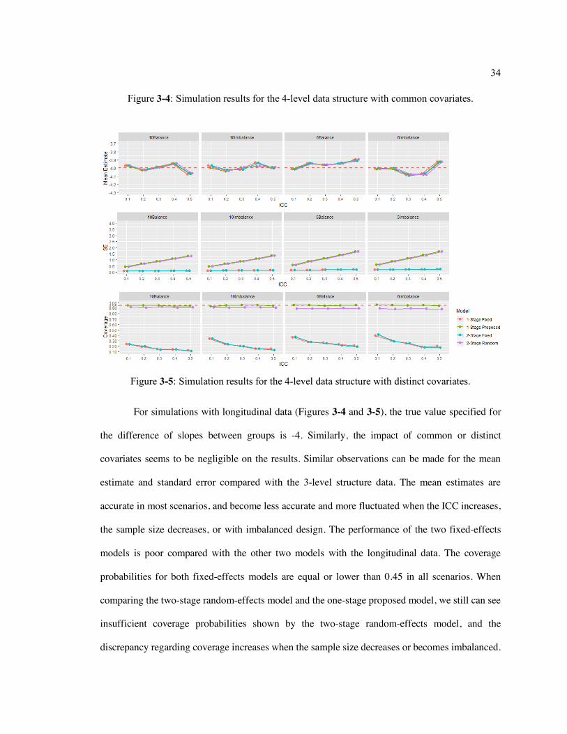
34

For simulations with longitudinal data (Figures 3-4 and 3-5), the true value specified for

the difference of slopes between groups is -4. Similarly, the impact of common or distinct

covariates seems to be negligible on the results. Similar observations can be made for the mean

estimate and standard error compared with the 3-level structure data. The mean estimates are

accurate in most scenarios, and become less accurate and more fluctuated when the ICC increases,

the sample size decreases, or with imbalanced design. The performance of the two fixed-effects

models is poor compared with the other two models with the longitudinal data. The coverage

probabilities for both fixed-effects models are equal or lower than 0.45 in all scenarios. When

comparing the two-stage random-effects model and the one-stage proposed model, we still can see

insufficient coverage probabilities shown by the two-stage random-effects model, and the

discrepancy regarding coverage increases when the sample size decreases or becomes imbalanced.

Figure 3-4: Simulation results for the 4-level data structure with common covariates.

Figure 3-5: Simulation results for the 4-level data structure with distinct covariates.

35

3.3.3 Supplemental Simulation Study

In the simulation study described above, we assume the random effects used to generate

simulated data are the same to that included in the proposed model. In this section, we conducted

an additional simulation study to evaluate situations that random effects used to generate the data

and the random effects used to fit the proposed model are different. We generated the simulated

data with 12 studies, balance sample size design, and common covariates. Only two sets of random

effects were included, 𝑟_)Líö and 𝑟Mì�)ìl . The mean function conditional on random effects for the

outcome variable is

𝐸-𝑌'M8|𝑟_)Líö, 𝑟Mì�)ìl1

= 220 − 8 × 𝑇𝑅𝑇 + 0.2 × 𝑏𝑎𝑠𝑒_𝑐ℎ𝑜 + 0.2 × 𝑎𝑔𝑒 − 4 × 𝑔𝑒𝑛𝑑𝑒𝑟 + 4× 𝑟𝑎𝑐𝑒$$

+ 6 × 𝑟𝑎𝑐𝑒&'_ − 0.8 × 𝑟𝑎𝑐𝑒()*ìl + 6× 𝑑𝑖𝑎𝑏𝑒𝑡𝑒𝑠 + 6× 𝐶𝑉𝐷 − 0.3× 𝑆𝑆zìõ�

+ 1.5× 𝑆𝑆_)í − 0.5 × 𝑜𝑟𝑑𝑒𝑟 + 𝑟_)Líö + 𝑟Mì�)ìl

Based on the simulated data, we fitted five test models as described in Table 3-3. Both two-stage

methods ignored the center-level random effect in the first stage. The one-stage proposed model

included three sets of random effects, with one redundant random effect rstudy_treatment.

Table 3-3: Model specifications of the supplemental simulation study. Test model Model fitting

two-stage fixed-effects 1st stage: study-level covariates, participant-level covariates;

2nd stage: a fixed-effects model to pool treatment effect

two-stage random-effects 1st stage: study-level covariates, participant-level covariates;

2nd stage: a random-effects model to pool treatment effect

one-stage fixed-effects participant-level covariates

one-stage proposed study-level covariates, participant-level covariates, rstudy,

rstudy_treatment, rcenter

36

We altered the ICC from 0.1, 0.2, to 0.5, and conducted 1000 simulations for each ICC

value. The simulation results are summarized in Table 3-4. The one-stage proposed model had a

higher chance in running into the convergence problem as it included a redundant random effect

term, and its variance was not able to be decided. In this case, it also indicates the need to remove

certain random effects. All the four test models provided similar coverage probabilities and mean

estimates, though the two-stage random-effects model still showed relatively insufficient coverage

probabilities compared with other methods.

Table 3-4: Results for the supplemental simulation study. ICC Model N Mean estimate SE Coverage

0.1 two-stage fixed-effects 1000 -7.998 0.383 0.950

one-stage proposed 565 -7.988 0.363 0.970

one-stage fixed-effects 1000 -7.996 0.392 0.965

two-stage random-effects 1000 -8.098 0.363 0.907
















37

3.4 Real Data Application

3.4.1 Example Data - Blood Pressure Studies

To assess the performance of the one-stage proposed model in a real setting, we selected 3

studies sponsored by the National Heart, Lung, and Blood Institute (NHLBI) to determine the effect

of reducing sodium intake on lowering blood pressure. The 3 studies identified are DASH-Sodium

(Sacks et al., 2001), PREMIER (Appel et al., 2003), and TOHP (phase II) (Trials of Hypertension

Prevention Collaborative Research Group, 1997), and the study information are summarized in

Table 3-5. IPD from each study were collected from the NHLBI website

(https://biolincc.nhlbi.nih.gov/home/).


Table 3-5: Study information summary of the NHLBI studies.

Study DASH-Sodium PREMIER TOHP (phase II)

Study period 1997-2002 1998-2004 1986-1998

Inclusion

SBP 120-159 mmHg; DBP 80-95 mmHg; free of anti-hypertensive medications


SBP <140 mmHg; DBP 83-89 mmHg; free of anti-hypertensive medications

Age range ³22 ³25 30-54

Study design crossover RCT; DASH diet + sodium reduction

parallel RCT; DASH diet + sodium reduction

parallel RCT; weight loss + sodium reduction

Study arms used low vs high (control) sodium level low vs control sodium level low vs control sodium level

Subjects used 204 541 1191

Number of centers 5 4 9

Outcome change of SBP after 1 month change of DBP after 1 month

change of SBP after 3 months change of DBP after 3 months

change of SBP after 6 months change of DBP after 6 months

SBP: systolic blood pressure; DBP: diastolic blood pressure; RCT: randomized clinical trial.

38

The 3 studies were designed as randomized clinical trials, comparing the effect on lowering

the blood pressure by combining treatment strategies of sodium intake reduction and weight loss

or DASH diet, targeting on the high-risk population of hypertension (Moore et al., 2011). The

normal blood pressure range is currently defined as systolic blood pressure (SBP) <120 mmHg and

diastolic blood pressure (DBP) <80 mmHg (World Health Organization, 2015). For the purpose of

this real data application, we did not include all treatment arms for analysis, and only focus on the

comparison of sodium intake reduction group versus control, advice only, or usual care. DASH-

Sodium had a crossover randomization design, and participants from DASH-Sodium were used as

self-comparison. The measurement times of the 3 studies were not the same, and we use the closest

measurement times between studies, which were the end of 1 month, 3 months, and 6 months for

DASH-Sodium, PREMIER, and TOHP, respectively. For the outcome variables, we focused on

the change of blood pressure from baseline to the selected end time point of each study, including

the change of systolic blood pressure (SBP) and the change of diastolic blood pressure (DBP).

Table 3-6: Model fitting with NHLBI studies.

Covariates DASH-sodium PREMIER TOHP (phase II) Participant-level Sodium level (low or control) X X X Age X X X Female X X X Race X X X Baseline SBP/DBP X X X Baseline weight X X X Study level

SS_mean X X X SS_std X X X Random effect

Study_treatment X X X Center X X X

SBP: systolic blood pressure; DBP: diastolic blood pressure.

39

We included participant-level variables, study-level variables, and random effects in the

one-stage proposed model (Table 3-6). For comparison, we calculated the individual treatment

effects estimated from each study. We also fitted the two-stage fixed-effects model, the two-stage

random-effects model, and the one-stage fixed-effects model to compare with the one-stage

proposed model. We conducted all analyses in SAS 9.4.

3.4.1 Results

The individual treatment effect estimates along with the overall estimates from the

proposed model and estimates from other meta-analysis models are presented in Figures 3-6 and

3-7 for the change of SBP. For the change of DBP, the results are presented in Figures 3-8 and 3-

9.

Figure 3-6: Individual and pooled estimates with outcome, the change of SBP.

40

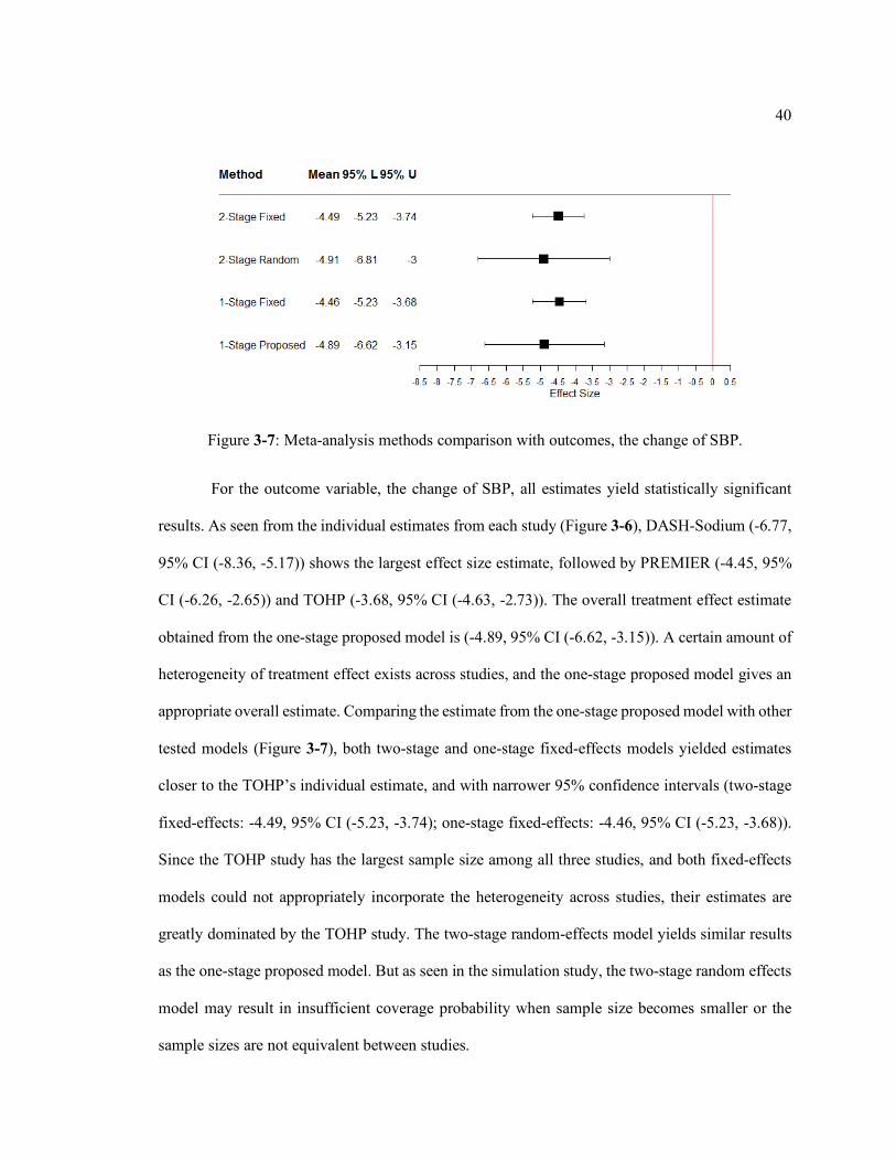
For the outcome variable, the change of SBP, all estimates yield statistically significant

results. As seen from the individual estimates from each study (Figure 3-6), DASH-Sodium (-6.77,

95% CI (-8.36, -5.17)) shows the largest effect size estimate, followed by PREMIER (-4.45, 95%

CI (-6.26, -2.65)) and TOHP (-3.68, 95% CI (-4.63, -2.73)). The overall treatment effect estimate

obtained from the one-stage proposed model is (-4.89, 95% CI (-6.62, -3.15)). A certain amount of

heterogeneity of treatment effect exists across studies, and the one-stage proposed model gives an

appropriate overall estimate. Comparing the estimate from the one-stage proposed model with other

tested models (Figure 3-7), both two-stage and one-stage fixed-effects models yielded estimates

closer to the TOHP’s individual estimate, and with narrower 95% confidence intervals (two-stage

fixed-effects: -4.49, 95% CI (-5.23, -3.74); one-stage fixed-effects: -4.46, 95% CI (-5.23, -3.68)).

Since the TOHP study has the largest sample size among all three studies, and both fixed-effects

models could not appropriately incorporate the heterogeneity across studies, their estimates are

greatly dominated by the TOHP study. The two-stage random-effects model yields similar results

as the one-stage proposed model. But as seen in the simulation study, the two-stage random effects

model may result in insufficient coverage probability when sample size becomes smaller or the

sample sizes are not equivalent between studies.

Figure 3-7: Meta-analysis methods comparison with outcomes, the change of SBP.

41

For the outcome variable, the change of DBP, all estimates still yield statistically

significant results though with a smaller effect size scale. As seen from the individual estimates

from each study (Figure 3-8), DASH-Sodium (-3.39, 95% CI (-4.47, -2.31)) shows the largest effect

size estimate, followed by TOHP (-2.75, 95% CI (-3.52, -1.98)) and PREMIER (-1.86, 95% CI (-

Figure 3-8: Individual and pooled estimates with outcome, the change of DBP.

Figure 3-9: Meta-analysis methods comparison with outcomes, the change of DBP.

42

3.16, -0.56)). The overall treatment effect estimate obtained from the one-stage proposed model is

(-2.63, 95% CI (-3.35, -1.92)). A certain amount of heterogeneity of treatment effect exists across

studies, but the four tested models present small differences regarding the mean estimate (Figure

3-7). This may due to the study with the largest sample size, TOHP, having an intermediate estimate

among the three individual estimates, so both fixed-effects models seem to yield reasonable overall

estimates. The one-stage proposed model gives an appropriate overall estimate. When comparing

the estimate from the one-stage proposed model with other tested models, both two-stage and one-

stage fixed-effects models still show narrower 95% confidence intervals (two-stage fixed-effects:

-2.76, 95% CI (-3.32, -2.19); one-stage fixed-effects: -2.74, 95% CI (-3.48, -1.99)). Little difference

is observed between the results of the two-stage random-effects model and the one-stage proposed

model (two-stage random-effects: -2.74, 95% CI (-3.48, -1.99)).

43

Chapter 4

The One-Stage Multi-Level Mixed-Effects Model for IPD Meta-Analysis with Outcomes from An Exponential Family

In the previous chapter, we proposed an IPD meta-analysis method for data with a

continuous outcome. But in practice, it also is very common to have data with other types of

outcomes, such as binary and count outcomes. In this chapter, we extend the previous work to

accommodate outcomes from an exponential family, which can greatly expand the application

range of the method. If the primary outcome variable has a distribution from the exponential family

(e.g., binary, binominal, Poisson, negative binominal with a fixed scale parameter, exponential,

gamma, beta, central t, etc.), then we can invoke a generalized linear mixed-effects model (GLMM)

(Breslow et al., 1993; Diggle et al., 2002; Karim et al., 1992; McCulloch et al., 2001).

4.1 Methods

4.1.1 Model Introduction

The GLMM is comprised of a generalized linear model with normal random effects. Let

𝑌'8(𝑡) denote the outcome variable measured at time 𝑡 for the 𝑙)* participant within the 𝑘)* study,

𝑘 = 1, 2, … , 𝐾 and 𝑙 = 1, 2, … , 𝑛' . We assume that a monotonic link function, 𝑔, of the expected

value of 𝑌'8(𝑡), conditional on the fixed-effect parameters and the random-effect parameters, can

be expressed as a linear predictor, i.e.,

𝑔[𝐸{𝑌'8(𝑡)|𝒙L,'8< (𝑡), 𝜷L', 𝒙M,'8< (𝑡), 𝜷M, 𝒛'8(𝑡), 𝜸'8, 𝒙'∗ ,𝜷∗, 𝒛'∗ , 𝜸'∗ }]

= 𝒙L,'8< (𝑡)𝜷L' + 𝒙M,'8< (𝑡)𝜷M + 𝒛'8< (𝑡)𝜸'8 + 𝒙'∗<𝜷∗ + 𝒛'∗<𝜸'∗

where

44

• 𝒙L,'8(𝑡) is a participant-level, unique fixed-effects, 𝑟L' × 1vector of design effects and


• 𝜷L' is a participant-level, unique fixed-effects 𝑟L' × 1 vector of parameters for the 𝑘)*

study

• 𝒙M,'8(𝑡) is a participant-level, common fixed-effects, 𝑟M × 1vector of design effects and


• 𝜷M is a participant-level, common fixed-effects 𝑟M × 1 vector of parameters

• 𝒛'8(𝑡) is a participant-level, random-effects 𝑠' × 1vector of design effects and covariates

at time 𝑡 for the 𝑙)* participant within the 𝑘)* cohort study

• 𝜸'8 is a participant-level, random-effects 𝑠' × 1 vector of parameters for the 𝑙)*

participant within the 𝑘)* cohort study

• 𝒙'∗ is a cohort-level, fixed-effects, 𝑟∗ × 1vector of design effects and covariates for the

𝑘)* cohort study

• 𝜷∗ is a cohort-level, fixed-effects 𝑟∗ × 1 vector of parameters for the 𝑘)* cohort study

• 𝒛'∗ is a cohort-level, random-effects 𝑠∗ × 1vector of design effects and covariates for the

𝑘)* cohort study

• 𝜸'∗ is a cohort-level, random-effects 𝑠∗ × 1 vector of parameters for the 𝑘)* cohort study

• the 𝜸'8’s are independent with 𝜸'8~𝑁R𝐤(𝟎, 𝚪'), where 𝚪' is a positive definite matrix

• the 𝜸'∗ ’s are independent with 𝜸'∗ ~𝑁_∗(𝟎, 𝚪∗), where 𝚪∗ is a positive definite matrix

• the 𝜸'8’s and the 𝜸'∗ ’s are mutually independent

Conditional on random effects 𝜸'8 and 𝜸'∗ , the 𝑌'8(𝑡)’s are independent, with a density

from the exponential family

45

𝑓(𝑌'8(𝑡)|𝜸'8, 𝜸'∗ ) = exp{

𝑌'8(𝑡)𝜃'8) − 𝑏(𝜃'8))𝑎'8)(𝜙)

+ 𝑐(𝑌'8(𝑡),𝜙)}

where 𝜃'8) is known as the canonical parameter, 𝜙 is a fixed dispersion parameter, 𝑎'8)(∙)

is some specific function of 𝜙, and 𝑏(∙) is some specific function of 𝜃'8) . The forms of 𝑎'8)(∙) and

𝑏(∙) depend on the distribution of the outcome. There are two properties of outcomes from the

exponential family, described as follows:

𝐸(𝑌'8(𝑡)|𝜸'8, 𝜸'∗ ) = 𝜇'8) = 𝑏�(𝜃'8))

𝑉𝑎𝑟(𝑌'8(𝑡)|𝜸'8, 𝜸'∗ ) = 𝑏��(𝜃'8))𝑎'8)(𝜙)

Parameter estimation proceeds by maximizing the marginal likelihood

𝐿(𝜷LX, … , 𝜷L�, 𝜷M, 𝜷∗, 𝝃|𝒀), which is constructed by integrating the full likelihood function with

respect to the distribution of the random effects

𝐿(𝜷LX, … , 𝜷L�, 𝜷M, 𝜷∗, 𝝃|𝒀) =��𝑓(𝒀'8; 𝜷L', 𝜷M, 𝜷∗, 𝝃)

�Z

8�X

�

'�X

=�9:;�:𝑓(𝒀'8|𝜷L', 𝜷M, 𝜷∗, 𝝃, 𝜸'8, 𝜸'∗ )𝑓(𝜸'8|𝝃)𝑑𝜸'8

�Z

8�X

<𝑓(𝜸'∗ |𝝃)𝑑𝜸'∗=�

'�X

where 𝝃 is the vector of variance-covariance parameters. However, if the link function is not linear,

the marginal likelihood can become intractable, and approximation of the integral, such as

linearization methods (quasi-likelihood methods), Laplace’s method, and numerical

approximation, are necessary.

There are two general types of integral approximation for GLMMs with normally

distributed random effects. The first type is to approximate the integrand, so that the integral of the

approximation has a closed form, which is also called analytical integration. The two typical

approaches are quasi-likelihood methods (Breslow et al., 1993; Diggle et al., 2002; Karim et al.,

1992; McCulloch et al., 2001; Wolfinger et al., 1993) and Laplace’s method (Tuerlinckx et al.,

2006). The quasi-likelihood methods include penalized quasi-likelihood (PQL) and marginal quasi-

46

likelihood (MQL). The second type of integral approximation for GLMMs is to approximate the

integral numerically. The typical approaches are Gauss quadrature (McCulloch et al., 1993;

Tuerlinckx et al, 2006), simulated maximum likelihood method (McCulloch et al., 1993;

Tuerlinckx et al, 2006; McCulloch et al., 1997), and the expectation-maximization (EM) algorithm

(McCulloch et al., 1997; Tuerlinckx et al, 2006; McCulloch et al., 1997). The following sections

introduce the methods separately. In the analysis of the simulation study and the real data

application, we will invoke PQL to obtain the estimates of fixed effects and variance-covariance

parameters.

4.1.2 Quasi-likelihood Methods

1) Penalized Quasi-likelihood (PQL)

Instead of defining a specific distribution, only conditional means and variances are defined

in PQL. Given random effects 𝜸'8 and 𝜸'∗ , the 𝑌'8(𝑡) are conditionally independent with means

𝐸[𝑌'8(𝑡)|𝜸'8, 𝜸'∗ ] = 𝜇'8)

and variances

𝑉𝑎𝑟[𝑌'8(𝑡)|𝜸'8, 𝜸'∗ ] = 𝑎'8)(𝜙)𝑣(𝜇'8)) = 𝑎'8)(𝜙)𝑣'8),

where 𝑣(∙) is a specific function of 𝜇'8) depending on the distribution of the outcome. The

conditional mean is related to a linear predictor 𝜂'8) through a link function 𝑔(∙):

𝑔(𝜇'8)) = 𝜂'8) = 𝒙L,'8< (𝑡)𝜷L' + 𝒙M,'8< (𝑡)𝜷M + 𝒛'8< (𝑡)𝜸'8 + 𝒙'∗<𝜷∗ + 𝒛'∗<𝜸'∗

By stacking 𝑔(𝜇'8)), we construct

𝑔(𝝁'8) = W𝑿L,'8 𝑿M,'8 𝟏YZ[×X𝒙'∗<\ d

𝜷L'𝜷M𝜷∗

e + W𝒁'8 𝟏YZ[×X𝒛'∗<\ g𝜸'8𝜸'∗h

and

47

𝑔(𝝁') = i

𝑔(𝝁'X)⋮

𝑔-𝝁'�Z1k

�∑ YZ[�Z[�� ×X

= i𝑿L,'X⋮

𝑿L,'�Zk

�∑ YZ[�Z[�� ×lmZ

𝜷L'lmZ×X

+ i𝑿M,'X 𝟏YZ�×X𝒙'

∗<

⋮ ⋮𝑿M,'�Z 𝟏YZ�Z×X𝒙'

∗<k

�∑ YZ[�Z[�� ×(lonl∗)

�𝜷M𝜷∗�(lonl∗)×X

+ i𝒁'X ⋯ 0⋮ ⋱ ⋮0 ⋯ 𝒁'�Z

𝟏YZ�×X𝒛'

∗<

⋮𝟏YZ�Z×X𝒛'

∗<k

�∑ YZ[�Z[�� ×(_Z×�Zn_∗)

�

𝜸'X⋮

𝜸'�Z𝜸'∗

�

(_Z×�Zn_∗)×X

= 𝑿L,'𝜷L' + 𝑿'𝜷 + 𝒁'𝜸'

where

𝜸'~𝑁_Z×�Zn_∗(𝟎,𝑮'(𝝃) = �

𝚪'⋮⋮0

…⋱⋯…

…⋮𝚪'…

0⋮⋮𝚪∗�).

Then, the marginal likelihood is approximated by the quasi-likelihood (QL), which is used

to estimate 𝜷L', 𝜷, and 𝝃:

𝐿(𝜷L', 𝜷, 𝝃|𝒀) =�:𝑓(𝒀'|𝜸',𝜷L', 𝜷)

�

'�X

𝑓(𝜸'; 𝝃)𝑑𝜸'

=�:��𝑓(𝑌'8(𝑡)|𝜸',𝜷L', 𝜷)YZ[

)�X

�Z

8�X

�

'�X


≈�:exp i��𝑄(𝑌'8(𝑡); 𝜇'8))YZ[

)�X

�Z

8�X

k |𝑮'|�X0 exp �−

12𝜸'<𝑮'�X𝜸'�

�

'�X

𝑑𝜸'

=�|𝑮'|�X0:exp i��𝑄(𝑌'8(𝑡); 𝜇'8))

YZ[

)�X

�Z

8�X

k exp �−12𝜸'<𝑮'�X𝜸'�

�

'�X

𝑑𝜸'

where 𝑄(𝑌'8(𝑡); 𝜇'8)) = ∫ CZ[())�LõZ[D(E)pZ[D

FZ[DCZ[())

𝑑𝑢 is the quasi-likelihood for 𝑌'8(𝑡) In this case,

∑ ∑ 𝑄(𝑌'8(𝑡); 𝜇'8))YZ[)�X

�Z8�X represents the true log-likelihood of the data.

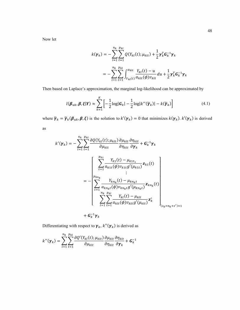
48

Now let

𝑘(𝜸') = −��𝑄(𝑌'8(𝑡); 𝜇'8))

YZ[

)�X

�Z

8�X

+12𝜸'<𝑮'�X𝜸'

= −��:𝑌'8(𝑡) − 𝑢𝑎'8)(𝜙)𝑣'8)

FZ[D

CZ[())𝑑𝑢

YZ[

)�X

�Z

8�X

+12𝜸'<𝑮'�X𝜸'

Then based on Laplace’s approximation, the marginal log-likelihood can be approximated by

𝑙(𝜷L', 𝜷, 𝝃|𝒀) ≈��−

12log|𝑮'| −

12log|𝑘��(𝜸ô')| − 𝑘(𝜸ô')�

�

'�X

(4.1)

where 𝜸ô' = 𝜸ô'(𝜷L', 𝜷, 𝝃) is the solution to 𝑘′(𝜸') = 0 that minimizes 𝑘(𝜸'). 𝑘′(𝜸') is derived

as

𝑘�(𝜸') = −��

𝜕𝑄(𝑌'8(𝑡); 𝜇'8))𝜕𝜇'8)

𝜕𝜇'8)𝜕𝜂'8)

𝜕𝜂'8)𝜕𝜸'

YZ[

)�X

�Z

8�X

+ 𝑮'�X𝜸'

= −

⎣⎢⎢⎢⎢⎢⎢⎢⎢⎡ �

𝑌'X(𝑡) − 𝜇'X)�𝑎'X)(𝜙)𝑣'X)𝑔′(𝜇'X))

𝒛'X(𝑡)YZ�

)�X⋮

�𝑌'�Z(𝑡) − 𝜇'�Z)

𝑎'�Z)(𝜙)𝑣'�Z)𝑔′(𝜇'�Z))𝒛'�Z(𝑡)

YZ�Z

)�X

��𝑌'8(𝑡) − 𝜇'8)

𝑎'8)(𝜙)𝑣'8)𝑔′(𝜇'8))𝒛'∗

YZ[

)�X

�Z

8�X ⎦⎥⎥⎥⎥⎥⎥⎥⎥⎤

(_Z×�Zn_∗)×X

+ 𝑮'�X𝜸'

Differentiating with respect to 𝜸', 𝑘′′(𝜸') is derived as

𝑘��(𝜸') =��𝜕𝑄′(𝑌'8(𝑡); 𝜇'8))

𝜕𝜇'8)𝜕𝜇'8)𝜕𝜂'8)

𝜕𝜂'8)𝜕𝜸'

YZ[

)�X

�Z

8�X

+ 𝑮'�X

49

=

⎣⎢⎢⎢⎢⎢⎡�

𝒛'X(𝑡)𝒛'X(𝑡)<

𝑎'X)(𝜙)𝑣'X)[𝑔�(𝜇'X))]0

YZ�

)�X

⋯ 0

⋮ ⋱ ⋮

0 ⋯ ��𝒛'∗ 𝒛'∗

<

𝑎'8)(𝜙)𝑣'8)[𝑔�(𝜇'8))]0

YZ[

)�X

�Z

8�X ⎦⎥⎥⎥⎥⎥⎤

+

⎣⎢⎢⎢⎢⎢⎡�-𝑌'X(𝑡) − 𝜇'X)�1𝒛'X(𝑡)

𝜕𝜕𝜸'

Ò1

𝑎'X)(𝜙)𝑣'X)𝑔�(𝜇'X))Ô

YZ�

)�X

⋯ 0

⋮ ⋱ ⋮

0 ⋯ ��(𝑌'8(𝑡) − 𝜇'8))𝒛'∗𝜕𝜕𝜸'

Ò1

𝑎'8)(𝜙)𝑣'8)𝑔�(𝜇'8))Ô

YZ[

)�X

�Z

8�X ⎦⎥⎥⎥⎥⎥⎤

+ 𝑮'�X

= 𝒁'<𝑾'𝒁' + 𝑹' + 𝑮'�X

≈ 𝒁'<𝑾'𝒁' + 𝑮'�X

where 𝑾' = 𝑑𝑖𝑎𝑔 � XõZ[D(E)pZ[D[I�(FZ[D)]´

� , 𝑙 = 1,… , 𝑛' and 𝑡 = 1,… , 𝑝'8 , is the

-∑ 𝑝'8�Z8�X 1 × -∑ 𝑝'8

�Z8�X 1 diagonal matrix that can be recognized as generalized linear model (GLM)

iterated weights. 𝑹' is the reminder term that has expectation 0 and has lower order than the terms

𝒁'<𝑾'𝒁' and 𝑮'�X. By ignoring 𝑹' and replacing 𝑘(𝜸ô') and 𝑘′′(𝜸ô') in 𝑙(𝜷L', 𝜷, 𝝃|𝒀),

𝑙(𝜷L', 𝜷, 𝝃|𝒀) ≈��−

12log|𝑮'| −

12log|𝑘��(𝜸ô')| − 𝑘(𝜸ô')�

�

'�X

= �i−12log|𝑮'| −

12logÏ𝒁'<𝑾'𝒁' + 𝑮'�XÏ +��𝑄(𝑌'8(𝑡); 𝜇'8))

YZ[

)�X

�Z

8�X

�

'�X

−12𝜸ô'<𝑮'�X𝜸ô'k

= �i−12logÏ𝒁'<𝑾'𝒁'𝑮' + 𝑰Ï +��𝑄(𝑌'8(𝑡); 𝜇'8))

YZ[

)�X

�Z

8�X

−12𝜸ô'<𝑮'�X𝜸ô'k

�

'�X

(4.2)

Assuming (𝒁'<𝑾'𝒁'𝑮' + 𝑰) varies slowly since the iterative weights vary slowly as a

function of the mean, we ignore the first term in (4.2). Therefore, the PQL can be defined as

50

𝑃𝑄𝐿 = �i��𝑄(𝑌'8(𝑡); 𝜇'8))

YZ[

)�X

�Z

8�X

−12𝜸'<𝑮'�X𝜸'k

�

'�X

(4.3)

The estimates -𝜷ÍL', 𝜷Í, 𝜸K1 = -𝜷ÍL'(𝝃), 𝜷Í(𝝃), 𝜸K(𝝃)1 can be obtained by jointly maximizing

the PQL in (4.3). Differentiation of PQL with respect to 𝜷 and 𝜸' leads to the score equations:

𝜕𝑃𝑄𝐿𝜕𝜷L'

=��(𝑌'8(𝑡) − 𝜇'8))𝒙L,'8)𝑎'8)(𝜙)𝑣'8)𝑔′(𝜇'8))

YZ[

)�X

�Z

8�X

= 0 (4.4)

𝜕𝑃𝑄𝐿𝜕𝜷

= ��(𝑌'8(𝑡) − 𝜇'8))𝒙'8)𝑎'8)(𝜙)𝑣'8)𝑔′(𝜇'8))

YZ[

)�X

�Z

8�X

�

'�X

= 0 (4.5)

𝜕𝑃𝑄𝐿𝜕𝜸'

=��(𝑌'8(𝑡) − 𝜇'8))𝒛'8)𝑎'8)(𝜙)𝑣'8)𝑔′(𝜇'8))

YZ[

)�X

�Z

8�X

− 𝑮'�X𝜸' = 0𝑘 = 1,… , 𝐾 (4.6)

(4.4) - (4.6) can be solved through an iterated weighted least squares approach using a

linearization technique. Let

𝐸(𝒀'|𝜸') = 𝝁' = 𝑔�X-𝑿L,'𝜷L' + 𝑿'𝜷 + 𝒁'𝜸'1 = 𝑔�X(𝜼')

𝑉𝑎𝑟(𝒀'|𝜸') = 𝑬' = 𝑑𝑖𝑎𝑔(𝑎'8)(𝜙)𝑣'8))

Based on a first-order Taylor series expansion at the current estimates 𝜷L' = �̧�L' , 𝜷 = �̧�,

and 𝜸' = 𝜸ô',

𝒀' = 𝑔�X(𝜼ô') + Δ̧�X𝑿L,'-𝜷L' − �̧�L'1 + Δ̧�X𝑿'-𝜷 − �̧�1 + Δ̧�X𝒁'(𝜸𝒌 − 𝜸ô')

+ 𝜺'

where Δ̧�X = 𝑑𝑖𝑎𝑔 �IO�(𝜼Z)𝜼Z

|𝜼Z�𝜼ôZ� = 𝑑𝑖𝑎𝑔-𝑔�(𝝁ô')1�X

, and 𝑉𝑎𝑟(𝜺') = 𝑬' .

For observations within the 𝑘)* study, let

𝒀'∗ = Δ̧[𝒀' − 𝑔�X(𝜼ô')] + 𝑿L,'�̧�L' + 𝑿'�̧� + 𝒁'𝜸ô'

= 𝑿L,'𝜷L' + 𝑿'𝜷 + 𝒁'𝜸𝒌 + 𝜺'

𝑉𝑎𝑟(𝒀'∗ ) = Δ̧𝑉𝑎𝑟(𝒀')Δ̧< = 𝒁'𝑮'𝒁'< + Δ̧𝑬'Δ̧< = 𝒁'𝑮'𝒁'< +𝐖$�X

51

Thus, we can construct 𝒀∗ for all studies as

𝒀∗ = d𝒀X∗⋮𝒀�∗e = i

𝑿L,X ⋯ 0⋮ ⋱ ⋮0 ⋯ 𝑿L,�


𝜷LX⋮

𝜷L�𝜷

� + d𝒁X ⋯ 0⋮ ⋱ ⋮0 ⋯ 𝒁�


𝜺X⋮𝜺�e

= 𝑿𝜷È + 𝒁𝜸 + 𝜺

with 𝐸(𝒀∗) = 𝑿𝜷È and 𝑉𝑎𝑟(𝒀∗) = 𝒁𝑮𝒁𝑻 +𝑾�𝟏 , where 𝑮 = 𝑑𝑖𝑎𝑔(𝑮𝒌) and 𝑾�𝟏 =

𝑑𝑖𝑎𝑔(𝑾𝒌�𝟏)). Based on 𝒀∗, estimation can proceed and be solved as a linear mixed-effects model

(see chapter 3).

The iterations for solving a GLMM based on the PQL algorithm is as follows:

1) Obtain initial estimates �̧�L' , �̧�, and 𝜸ô;

2) Construct the pseudo outcome 𝒀∗ based on current estimates �̧�L' , �̧�, and 𝜸ô;

3) Update �̧�L' , �̧�, and 𝜸ô, and obtain the estimate 𝝃¹ by solving the GLM of 𝒀∗ (ML or REML);

4) Repeat 2) to 3) until convergence.

2) Marginal Quasi-likelihood (MQL)

The MQL method is similar to PQL method. It also starts with a first-order Taylor series

expansion, but the expansion is now at the current estimate for 𝜷L' = �̧�L', 𝜷 = �̧�, and 𝜸' = 𝟎.

Let

𝐸(𝒀') = 𝝁' = 𝑔�X-𝑿L,'𝜷L' + 𝑿'𝜷1 = 𝑔�X(𝜼'� )

Then, based on a first-order Taylor series expansion at the current estimate 𝜷L' = �̧�L',

𝜷 = �̧�, and 𝜸' = 𝟎,

𝒀' = 𝑔�X(𝜼'� ) + Δ̧�X𝑿L,'-𝜷L' − �̧�L'1 + Δ̧�X𝑿'-𝜷− �̧�1 + Δ̧�X𝒁'𝜸𝒌 + 𝜺'

52

where Δ̧�X = 𝑑𝑖𝑎𝑔(IO�-𝜼Z

� 1𝜼Z

� |𝜼Z� �𝜼ôZ� ) = 𝑑𝑖𝑎𝑔-𝑔�(𝝁ô')1�X

, and 𝑉𝑎𝑟(𝜺') = 𝑬' . For observations

within the 𝑘)* study, let

𝒀'∗ = Δ̧[𝒀' − 𝑔�X(𝜼ô'� )] + 𝑿L,'�̧�L' + 𝑿'�̧� = +𝑿L,'𝜷L' + 𝑿'𝜷 + 𝒁'𝜸𝒌 + 𝜺'

𝑉𝑎𝑟(𝒀'∗ ) = Δ̧𝑉𝑎𝑟(𝒀')Δ̧< = 𝒁'𝑮'𝒁'< + Δ̧𝑬'Δ̧< = 𝒁'𝑮'𝒁'< +𝐖$�X

Thus,

𝒀∗ = d𝒀X∗⋮𝒀�∗e = i

𝑿L,X ⋯ 0⋮ ⋱ ⋮0 ⋯ 𝑿L,�


𝜷LX⋮

𝜷L�𝜷

� + d𝒁X ⋯ 0⋮ ⋱ ⋮0 ⋯ 𝒁�


𝜺X⋮𝜺�e

= 𝑿𝜷È + 𝒁𝜸 + 𝜺

with 𝐸(𝒀∗) = 𝑿𝜷È and 𝑉𝑎𝑟(𝒀∗) = 𝒁𝑮𝒁𝑻 +𝑾�𝟏 , where 𝑮 = 𝑑𝑖𝑎𝑔(𝑮𝒌) and 𝑾�𝟏 =

𝑑𝑖𝑎𝑔(𝑾𝒌�𝟏)).

Again, it can be considered and solved as a linear mixed-effects model (see chapter 3). The

iterations for solving a GLMM based on the MQL algorithm is slightly different from that for PQL:

𝜸ô is not estimated at each iteration using the MQL, and instead, 𝜸ô will be estimated using BLUP

after convergence.

4.1.3 Laplace’s Method

Laplace’s method is usually used to approximate an integral of the form ∫ 𝑒8(𝒕)𝑑𝒕, which

requires 𝑙(𝒕) to be a smooth, bounded, and unimodal function. Starting from the marginal

likelihood function of a GLMM,

53

𝐿(𝜷L', 𝜷, 𝝃|𝒀) =�𝑓(𝒀';𝜷L', 𝜷, 𝝃)

�

'�X

=�:𝑓(𝒀', 𝜸';𝜷L', 𝜷, 𝝃)�

'�X

𝑑𝜸'

=�:𝑓(𝒀'|𝜸',𝜷L', 𝜷)�

'�X


=�:��𝑓(𝑌'8(𝑡)|𝜸',𝜷L', 𝜷)YZ[

)�X

�Z

8�X

�

'�X


∝�:|𝑮'|�X0exp{��log[𝑓(𝑌'8(𝑡)|𝜸', 𝜷L', 𝜷)]

YZ[

)�X

�Z

8�X

�

'�X

−12𝜸'<𝑮'�X𝜸'} 𝑑𝜸'

Let

𝑑(𝜸') = −��log[𝑓(𝑌'8(𝑡)|𝜸',𝜷L', 𝜷)]YZ[

)�X

�Z

8�X

+12𝜸'<𝑮'�X𝜸'

Then based on a second-order Taylor series expansion about 𝜸K' = 𝜸K'(𝜷L', 𝜷, 𝝃) at the

maximum values of 𝑑(𝜸') such that 𝑑�(𝜸K') = 0, we have

𝑑(𝜸') ≈ 𝑑(𝜸K') +12(𝜸' − 𝜸K')<𝑑��(𝜸K')(𝜸' − 𝜸K')

where 𝑑��(𝜸') is the Hessian matrix which contains the second-order partial derivatives of 𝑑(𝜸').

Then, ∫ exp[𝑑(𝜸')]𝑑𝜸'can be approximated as

:exp[𝑑(𝜸')]𝑑𝜸' ≈ :exp �𝑑(𝜸K') +12(𝜸' − 𝜸K')<𝑑��(𝜸K')(𝜸' − 𝜸K')�𝑑𝜸'

≈ exp[𝑑(𝜸K')]:exp �−12(𝜸' − 𝜸K')<-−𝑑��(𝜸K')1(𝜸' − 𝜸K')�𝑑𝜸'

≈ exp[𝑑(𝜸K')] (2𝜋)(_Z×�Zn_∗)/0|−𝑑��(𝜸K')|

�X0

and the marginal likelihood can be approximated by

54

𝑙(𝜷L', 𝜷, 𝝃|𝒀) ∝ � �−

12log|𝑮'| + 𝑑(𝜸K') +

12log|𝑑��(𝜸K')|�

�

'�X

Since 𝜃'8) is the canonical parameter, we have 𝜃'8) = 𝜂'8) = 𝑔(𝜇'8)). Therefore, 𝜸K' can

be solved via

𝑑�(𝜸') = −��𝜕 log[𝑓(𝑌'8(𝑡)|𝜸',𝜷L', 𝜷)]

𝜕𝜃'8)𝜕𝜂'8)𝜕𝜸'

YZ[

)�X

�Z

8�X

+ 𝑮'�X𝜸' = 𝟎

= −

⎣⎢⎢⎢⎢⎢⎡ ∑ CZ�())�ø�-SZ�D�1

õZ�D(E)𝒛'X(𝑡)

YZ�)�X

⋮

∑CZ�Z())�ø

��SZ�ZD�

õZ�ZD(E)𝒛'�Z(𝑡)

YZ�Z)�X

∑ ∑ CZ[())�ø�(SZ[D)õZ[D(E)

𝒛'∗YZ[)�X

�Z8�X ⎦

⎥⎥⎥⎥⎥⎤

(_Z×�Zn_∗)×X

+ 𝑮'�X𝜸' = 𝟎.

Meanwhile, the Hessian matrix 𝑑��(𝜸') can be estimated as

𝑑��(𝜸') =��𝜕{log[𝑓(𝑌'8(𝑡)|𝜸',𝜷L', 𝜷)]}′

𝜕𝜃'8)𝜕𝜂'8)𝜕𝜸'

YZ[

)�X

�Z

8�X

+ 𝑮'�X

=

⎣⎢⎢⎢⎢⎢⎡�

𝑏′′(𝜃'X)�)𝒛'X(𝑡)𝒛'X(𝑡)<

𝑎'X)(𝜙)

YZ�

)�X

⋯ 0

⋮ ⋱ ⋮

0 ⋯ ��𝑏′′(𝜃'8))𝒛'∗ 𝒛'∗

<

𝑎'8)(𝜙)

YZ[

)�X

�Z

8�X ⎦⎥⎥⎥⎥⎥⎤

+ 𝑮'�X

= 𝒁'<𝑸'𝒁' + 𝑮'�X

where 𝑸' = 𝑑𝑖𝑎𝑔 �ø��(SZ[D)õZ[D(E)

� , 𝑙 = 1,… , 𝑛' and 𝑡 = 1,… , 𝑝'8 , is the -∑ 𝑝'8�Z8�X 1 × -∑ 𝑝'8

�Z8�X 1

diagonal matrix. The estimates of 𝜷L' , 𝜷, and 𝝃 can be obtained through a Newton-Raphson or a

Fisher scoring algorithm. The estimates of 𝜸' can be obtained through BLUP after the convergence

of estimating 𝜷L' , 𝜷, and 𝝃.

55

4.1.3 Gaussian Quadrature

Another category of methods to approximate the integral of a function is to approximate

the integral numerically. This technique is useful when the function cannot be analytically

integrated or the analytical form of an integral is very complicated. Gaussian quadrature is one

typical approach. Let’s consider a general weighted integral ∫ 𝑓(𝑥)𝑤(𝑥)𝑑𝑥øõ , where 𝑤(𝑥) is a

weight function and is a continuous, non-negative function. Gaussian quadrature can approximate

the integral by a finite weighted sum based on 𝑚 selected nodes within the given domain (𝑎, 𝑏):

: 𝑓(𝑥)𝑤(𝑥)𝑑𝑥ø

õ≈� 𝑓(𝑥')𝐴'(𝑥')

z

'�X

where 𝑥' , 𝑖 = 1…𝑚 , are the nodes and 𝐴'(𝑥') are their corresponding weights. The theory on

Gaussian quadrature states that the 𝑚 nodes and their corresponding weights are optimally spaced

and calculated, such that the quadrature, the finite weighted sum, will exactly integrate any

polynomial with degree of 2𝑚 − 1.

1) Gauss-Hermite Quadrature

For GLMM, random effects are assumed to be normally distributed, and the numerical

integration is usually done through Gauss-Hermite quadrature. Gauss-Hermite quadrature can

approximate integrals of the form ∫ 𝑓(𝑥)𝑒�W𝟐𝑑𝑥 as follows:

:𝑓(𝑥)𝑒�W𝟐𝑑𝑥 ≈� 𝑓(𝑥')𝐴'(𝑥')

z

'�X

where 𝑥' and 𝐴'(𝑥') are the Gauss-Hermite quadrature nodes and weights that can be found in the

literature (Abramowitz et al., 1966; Golub et al.). The 𝑤(𝑥) here has a standard normal kernel

𝑒�W𝟐 . With some transformations, the approximation can be extended to the multivariate version

56

with random effects 𝒙X×X following a multivariate normal distribution with mean 𝝁 and variance-

covariance matrix 𝚺:

:𝑓(𝑦|𝒙)𝑓(𝒙|𝝁, 𝚺)𝑑𝑥 ≈ Ò1√𝜋ÔX� …z

ø��X

� 𝑓 Ò𝑦|𝒙ø∗ = 𝝁+ √2𝚺X0𝒙øÔ𝐴ø�-𝑥ø�1…𝐴øZ �𝑥øZ�

z

øZ�X

where 𝑚 is the number of nodes selected for each element of 𝒙, 𝒙ø = �𝑥ø�,… , 𝑥øZ�<

, 𝑥ø[ and

𝐴ø[-𝑥ø[1 are the node and the weight for the 𝑏')* node of the 𝑖)* random effect, respectively, based

on the Gauss-Hermite quadrature nodes and weights, 𝑖 = 1,… ,𝑄.

Under the GLMM framework with random effects 𝜸'~𝑁_Z×�Zn_∗(𝟎,𝑮'), the marginal

likelihood function can be approximated by

𝐿(𝜷, 𝝃|𝒀) =�:��𝑓(𝑌'8(𝑡)|𝜷L', 𝜷, 𝜸')

YZ[

)�X

�Z

8�X

�

'�X


≈� 9Ò1√𝜋ÔX

� …z

ø��X

� d�� 𝑓 Ò𝑌'8(𝑡)|𝜷L', 𝜷, 𝜸'∗ = √2𝑮'X0𝒙øÔ

YZ[

)�X

�Z

8�X

𝐴ø�-𝑥ø�1…𝐴øZ-𝑥øZ1ez

øZ�X

=�

'�X

where 𝑄 = 𝑠' × 𝑛' + 𝑠∗, 𝑚, 𝒙ø, and 𝐴ø[-𝑥ø[1 are defined similarly as above.

2) Adaptive Gauss-Hermite Quadrature

An improved method of Gauss-Hermite quadrature is adaptive Gauss-Hermite quadrature,

which selects Gauss-Hermite quadrature nodes differently for each study 𝑘 according to its most

likely value of random effects conditional on current estimates of �̧�L' , �̧�, and 𝝃¹. In other words,

the random effects of the studies will be centered and scaled differently. When the between-study

variance is large, more nodes (𝑚) will be needed in Gauss-Hermite quadrature to achieve an ideal

approximation. The advantage of adaptive Gauss-Hermite quadrature is that fewer nodes are

needed to achieve equivalent accuracy as for Gauss-Hermite quadrature. With a smaller 𝑚, the

placements of the 𝑚 nodes for each study will depend on its specific distribution of random effects.

57

Let

𝑎(𝜸'|𝑌'8(𝑡), 𝜷L', 𝜷, 𝝃) =��𝑓(𝑌'8(𝑡)|𝜷L', 𝜷, 𝜸')

YZ[

)�X

�Z

8�X

𝑓(𝜸'; 𝝃)

and 𝑎(𝜸'|𝑌'8(𝑡), 𝜷L', 𝜷, 𝝃) can be treated as the posterior distribution of random effects for the 𝑘)*

study. Therefore, for the 𝑘)* study, the estimate of 𝜸' = 𝜸K' = 𝜸K'(�̧�L', �̧�, 𝝃¹) can be obtained via

𝜕 log 𝑎(𝜸'|𝑌'8(𝑡), 𝜷L', 𝜷, 𝝃)𝜕𝜸'

|�̧�,𝝃¹ = 0

where �̧�L', �̧�, 𝝃¹ are the current estimates of 𝜷L', 𝜷, 𝝃. 𝑮' can also be estimated as 𝑮Í', using the

observed or expected information matrix

𝑮Í' = −𝜕0 log 𝑎(𝜸'|𝑌'8(𝑡), 𝜷L', 𝜷, 𝝃)

𝜕𝜸'𝜕𝜸'|𝜷ÍmZ,𝜷Í,𝝃&

or

𝑮Í' = 𝐸 v−𝜕0 log 𝑎(𝜸'|𝑌'8(𝑡), 𝜷L', 𝜷, 𝝃)

𝜕𝜸'𝜕𝜸'|𝜷ÍmZ,𝜷Í,𝝃&w

Then, the marginal likelihood can be approximated by

𝐿(𝜷L', 𝜷, 𝝃|𝒀) =�:��𝑓(𝑌'8(𝑡)|𝜷L', 𝜷, 𝜸')YZ[

)�X

�Z

8�X

�

'�X

𝑓(𝜸';𝝁 = 𝟎,𝚺 = 𝑮')𝑑𝜸'

=�:∏ ∏ 𝑓(𝑌'8(𝑡)|𝜷L', 𝜷, 𝜸')

YZ[)�X

�Z8�X 𝑓(𝜸'; 𝟎, 𝑮')

𝑓-𝜸'; 𝜸K',𝑮Í'1𝑓-𝜸'; 𝜸K',𝑮Í'1

�

'�X

𝑑𝜸'

≈�9Ò1√𝜋ÔX� …z

ø��X

� i��𝑓(𝑌'8(𝑡)|𝜷L', 𝜷, 𝜸'∗ )YZ[

)�X

�Z

8�X

𝑓(𝜸'∗ ; 𝟎, 𝑮')(2𝜋)X0Ï𝑮Í'Ï

X0exp(

12(𝜸'∗

z

øZ�X

�

'�X

− 𝜸K')<𝑮Í'�X(𝜸'∗ − 𝜸K'))𝐴ø�-𝑥ø�1…𝐴øZ �𝑥øZ�k=

Replacing nodes 𝜸'∗ with 𝜸K' + √2𝑮Í'�´𝒙ø,

58

𝐿(𝜷L', 𝜷, 𝝃|𝒀) ≈�9(2)

X0 Ï𝑮Í'Ï

X0 � …

z

ø��X

� i��𝑓 Õ𝑌'8(𝑡)|𝜷L', 𝜷, 𝜸K' + √2𝑮Í'X0𝒙øÖ

YZ[

)�X

�Z

8�X

𝑓 Õ𝜸K'

z

øZ�X

�

'�X

+ √2𝑮Í'X0𝒙ø;𝟎, 𝑮'Öexp(𝒙ø<𝒙ø)𝐴ø�-𝑥ø�1…𝐴øZ �𝑥øZ�k=

4.1.4 Simulated Maximum Likelihood

Simulated maximum likelihood estimation also is called Monte Carlo integration, which is

a stochastic numerical approximation to the integral. Starting with the marginal likelihood, it can

be written as

𝐿(𝜷L', 𝜷, 𝝃|𝒀) =�:��𝑓(𝑌'8(𝑡)|𝜷L', 𝜷, 𝜸')YZ[

)�X

�Z

8�X

�

'�X


=�:∏ ∏ 𝑓(𝑌'8(𝑡)|𝜷L', 𝜷, 𝜸')

YZ[)�X

�Z8�X 𝑓(𝜸'; 𝝃)

ℎ(𝜸'; 𝝃′)ℎ(𝜸'; 𝝃′)

�

'�X

𝑑𝜸'

where ℎ(𝜸') is defined as importance sampling distribution and it is known. Then

𝐿(𝜷L', 𝜷, 𝝃|𝒀) can be written as the product of expectations of ∏ ∏ î(CZ[())|𝜷mZ,𝜷,𝜸Z)

]Z[D��

�Z[�� î(𝜸Z;𝝃)

*(𝜸Z;𝝃�)

with respect to ℎ(𝜸'; 𝝃′) . Suppose we can randomly generate G independent samples,

𝜸'X , 𝜸'0,… , 𝜸'^ from ℎ(𝜸'; 𝝃′). Then 𝐿(𝜷L', 𝜷, 𝝃|𝒀) can be approximated by

𝐿(𝜷L', 𝜷, 𝝃|𝒀) =�:

∏ ∏ 𝑓(𝑌'8(𝑡)|𝜷L', 𝜷, 𝜸')YZ[)�X

�Z8�X 𝑓(𝜸'; 𝝃)

ℎ(𝜸'; 𝝃�)ℎ(𝜸'; 𝝃�)

�

'�X

𝑑𝜸'

≈�i1𝐺�

∏ ∏ 𝑓-𝑌'8(𝑡)|𝜷L', 𝜷, 𝜸'I1YZ[

)�X�Z8�X 𝑓-𝜸'

I; 𝝃1ℎ-𝜸'

I; 𝝃′1

^

I�X

k�

'�X

The efficiency of the approximation depends on the choice of ℎ(𝜸'; 𝝃′). In practice,

ℎ(𝜸'; 𝝃′) is suggested to be chosen close to 𝑓(𝜸'; 𝝃), and it should be feasible and efficient to draw

59

simulated samples. Similar with adaptive Gauss-Hermite quadrature, ℎ(𝜸'; 𝝃′) can be chosen as

the posterior distribution of random effects for 𝑘)* study. Let ℎ(𝜸'; 𝝃′) = 𝑓-𝜸'; 𝜸K',𝑮Í'1 , and

𝜸K', 𝑮Í' are defined as above. Therefore, 𝐿(𝜷L', 𝜷, 𝝃|𝒀) can be approximated as

𝐿(𝜷L', 𝜷, 𝝃|𝒀)

=�:∏ ∏ 𝑓(𝑌'8(𝑡)|𝜷L', 𝜷, 𝜸')

YZ[)�X

�Z8�X 𝑓(𝜸'; 𝟎, 𝑮')

𝑓-𝜸'; 𝜸K',𝑮Í'1𝑓-𝜸'; 𝜸K',𝑮Í'1

�

'�X

𝑑𝜸'

≈�i1𝐺�

∏ ∏ 𝑓-𝑌'8(𝑡)|𝜷L', 𝜷, 𝜸'I1YZ[

)�X�Z8�X 𝑓-𝜸'

I;𝟎, 𝑮'1𝑓-𝜸'

I; 𝜸K',𝑮Í'1

^

I�X

k�

'�X

Again, it can be treated as the product of expectations of ∏ ∏ î(CZ[())|𝜷mZ,𝜷,𝜸Z)

]Z[D��

�Z[�� î(𝜸Z;𝟎,𝑮Z)

î-𝜸Z;𝜸KZ,𝑮ÍZ1

of the normally distributed random effects 𝜸'.

4.1.4 Expectation-Maximization (EM) algorithm

In this approach, the complete data consist of the response outcome 𝒀' and the random

effects 𝜸' , 𝑘 = 1, 2, … , 𝐾 . If the random effects were known, we can construct the complete

likelihood as

𝐿M(𝜷L', 𝜷, 𝝃|𝒀, 𝜸) =�9��𝑓(𝑌'8(𝑡)|𝜷L', 𝜷, 𝜸')

YZ[

)�X

�Z

8�X

𝑓(𝜸'; 𝝃)=�

'�X

However, random effects cannot be observed in practice, and instead we can estimate the

expectation of 𝐿M(𝜷L', 𝜷, 𝝃|𝒀, 𝜸) based on the current estimates �̧�L', �̧� , and 𝝃¹ , and response

outcome 𝒀'. Therefore, the expectation of the complete log-likelihood 𝑙M-𝜷L', 𝜷, 𝝃Ï𝒀, 𝜸, �̧�L', �̧�, 𝝃¹1

can be estimated via

60

𝐸 �𝑙M-𝜷L', 𝜷, 𝝃Ï𝒀,𝜸, �̧�L', �̧�, 𝝃¹1�

= 𝐸 9� 9��log[𝑓(𝑌'8(𝑡)|𝜷L', 𝜷, 𝜸')]YZ[

)�X

�Z

8�X

+ 𝑙𝑜𝑔𝑓(𝜸'; 𝝃)=�

'�X

=

=�:9��log[𝑓(𝑌'8(𝑡)|𝜷L', 𝜷, 𝜸')]YZ[

)�X

�Z

8�X

�

'�X

+ 𝑙𝑜𝑔𝑓(𝜸'; 𝝃)=𝑝(𝜸';𝒀𝒌, �̧�L', �̧�, 𝝃¹)𝑑𝜸' (4.7)

where 𝑝(𝜸';𝒀, �̧�L', �̧�, 𝝃¹) is the conditional density of the random effects given �̧�L' , �̧�, and 𝝃¹, and

𝒀', which can be replaced by the posterior distribution of 𝜸', such as

𝑝-𝜸';𝒀, �̧�L', �̧�, 𝝃¹1 ∝��𝑓-𝑌'8(𝑡)|�̧�L', �̧�, 𝜸'1

YZ[

)�X

�Z

8�X

𝑓-𝜸'; 𝝃¹1 (4.8)

Once (4.7) is obtained, it is maximized as a function of 𝜷L' , 𝜷 and 𝝃, and the new estimates

�̧�L' , �̧� , 𝝃¹ will be updated. The algorithm is iterated between the expectation step and the

maximization step until the convergence of observed likelihood function 𝐿(𝜷L', 𝜷, 𝝃|𝒀) or

parameter estimates 𝜷L' , 𝜷 and 𝝃.

Since both parts of the integrals in (4.7) do not have closed forms, the approximation of

the integral still relies on Gaussian quadrature or simulated maximum likelihood method. In the

latter method, we can randomly generate G independent samples, 𝜸'X , 𝜸'0, … , 𝜸'^ from (4.8). Then

maximizing (4.7) is equivalent to maximizing

� 91𝐺i��logW𝑓-𝑌'8(𝑡)|𝜷L', 𝜷, 𝜸'

I1\YZ[

)�X

�Z

8�X

+ 𝑙𝑜𝑔𝑓-𝜸'I; 𝝃1k=

�

'�X

.

61

4.2 Inference for Fixed Effects 𝜷

In hypothesis testing, large sample tests regarding fixed effects 𝜷 can be performed in

GLMM, and related confidence intervals estimated, by using a Wald chi-square test, a likelihood

ratio test or a score test. For a contrast matrix 𝑳à×_ where 𝑀 ≤ 𝑃 , we want to test the null

hypothesis 𝐻â: 𝑳𝜷 = 𝟎 versus 𝐻X: 𝑳𝜷 ≠ 𝟎.

1) Wald Chi-square Test

Based on the final estimate 𝜷Í , its estimated covariance matrix can be obtained via either the

observed or expected information matrix 𝐼𝜷Í , evaluated at 𝜷Í

𝑰𝜷Í = −

´8�𝜷, 𝜷ÍL', 𝛏&ñ𝒀�𝛃𝛃ò

|𝜷�𝜷Í or 𝑰𝜷Í = 𝐸(−´8�𝜷, 𝜷ÍL', 𝛏&ñ𝒀�

𝛃𝛃ò|𝜷�𝜷Í)

where 𝛏& is the estimate of 𝛏. To test the null hypothesis, the Wald statistic is

𝐶0 = -𝑳𝜷Í1<a𝑳𝑰𝜷Í

�X𝑳𝑻b�X-𝑳𝜷Í1

and compare 𝐶0 to a 𝜒à0 distribution. If 𝑀, the number of rows of 𝑳, equals 1, then an approximate

(1 − 𝛼) × 100% confidence interval for 𝑳𝜷 is given by 𝑳𝜷Í ± 𝑧X�é/0ê𝑳𝑰𝜷Í�X𝑳𝑻. Similar to linear

mixed-effects model, we can convert to an approximate 𝐹 distribution in the presence of a small

sample size.

2) Likelihood Ratio Test

One alternative to the Wald test is the likelihood ratio test (LRT). Denote the maximized

ML log-likelihoods under null and alternative hypotheses as 𝑙6lìíLMìí(�̧�) and 𝑙6îL88(𝜷Í). The LRT

for two nested models can be constructed by comparing 𝑙6lìíLMìí(�̧�) and 𝑙6îL88(𝜷Í). The larger the

62

difference between 𝑙6lìíLMìí(�̧�) and 𝑙6îL88(𝜷Í), the stronger the evidence that the reduced model is

inadequate. The LRT statistic is

𝐺0 = −2(𝑙6lìíLMìí(�̧�) − 𝑙6îL88(𝜷Í))

and compare 𝐺0 to a 𝜒à0 distribution. If 𝑀, the number of rows of 𝑳, equals 1, then an approximate

(1 − 𝛼) × 100% confidence interval for 𝑳𝜷 can also be obtained by inverting the LRT.

3) Score Test

A score test is based on the null hypothesis, and the score function is obtained at 𝜷 = �̧�:

𝒖-�̧�1 =𝜕𝑙-𝜷, �̧�L', 𝛏¹Ï𝒀1

𝜕𝛃|𝜷��̧�

The information matrix 𝑰𝜷 can be either the observed or expected information matrix as defined

above, but it is also evaluated at 𝜷 = �̧�. The score test statistic is defined as

𝑠-�̧�1 = 𝒖-�̧�1<𝑰�̧��X𝒖-�̧�1

𝑠-�̧�1 is compared to a 𝜒à0 distribution If 𝑀 equals 1, then an approximate (1 − 𝛼) × 100%

confidence interval for 𝑳𝜷 can also be obtained by inverting the score test.

4.3 Simulation Study

4.3.1 Simulation Design

We performed a simulation study to assess the proposed one-stage model for IPD meta-

analysis with binary outcomes. The simulated data were generated in the settings of multi-center

clinical trials, with a two-arm, placebo-controlled, parallel design, which aimed to detect whether

the treatment could reduce a patient’s total cholesterol level. The observed outcome variable is a

63

binary outcome, with specifying cholesterol level ³200 mg/dL as high and <200 mg/dL as low. We

designed the simulated data to have a 3-level or a 4-level structure (Figure 3-1) based on a logistic

link function. For the 3-level data, we assume the clinical data were collected from multiple studies,

and each study had different numbers of centers (study sites), and each center had different numbers

of participants. For the 4-level data, we assumed each participant within a center had different

numbers of visits, which was the visit level and leads to longitudinal data for the participant. For

both 3-level and 4-level multi-center data, we simulated several participant-level variables,

including treatment assignment (TRT; placebo or active treatment), baseline cholesterol level

(base_cho; mg/dL), age at enrollment, gender (male or female), race (Caucasian (Cau), African

American (AA), Hispanic (His) and other), diabetes disease status (yes or no), and cardiovascular

disease status (CVD; yes or no). Both base_cho and age were centered by their population means,

respectively. We generated two sets of study-level random effects, including study-level random

intercept (rstudy) and random effect for treatment effects across studies (rstudy_treatment). We imposed

another two sets of random effects to the center level, including center-level random intercept

(rcenter) and random effect for baseline cholesterol level (rcenter_bc). The primary parameter of interest

is the difference in treatment between treatment groups (log odds ratio) with the 3-level data. With

the 4-level data structure, we generated each participant’s weight (lbs) as a repeated measurement

variable, and each participant might have 3 to 5 visits. Weight was centered by its population mean

before it was used. We included another set of random intercepts for participant level (rparticipant),

but removed the random effect for baseline cholesterol level (rcenter_bc) and replaced the rstudy_treatment

with the random effect for the interaction between treatment effects and visit (rstudy_treatment*visit). The

primary parameter of interest is the difference in slopes between treatment groups (log odds ratio)

with the 4-level data. The continuous outcome variable is firstly generated based on (3.14) and

(3.15) with the absolute values of coefficients divided by 10, and then it was dichotomized as a

binary variable based on the cutoff level 200 mg/dL.

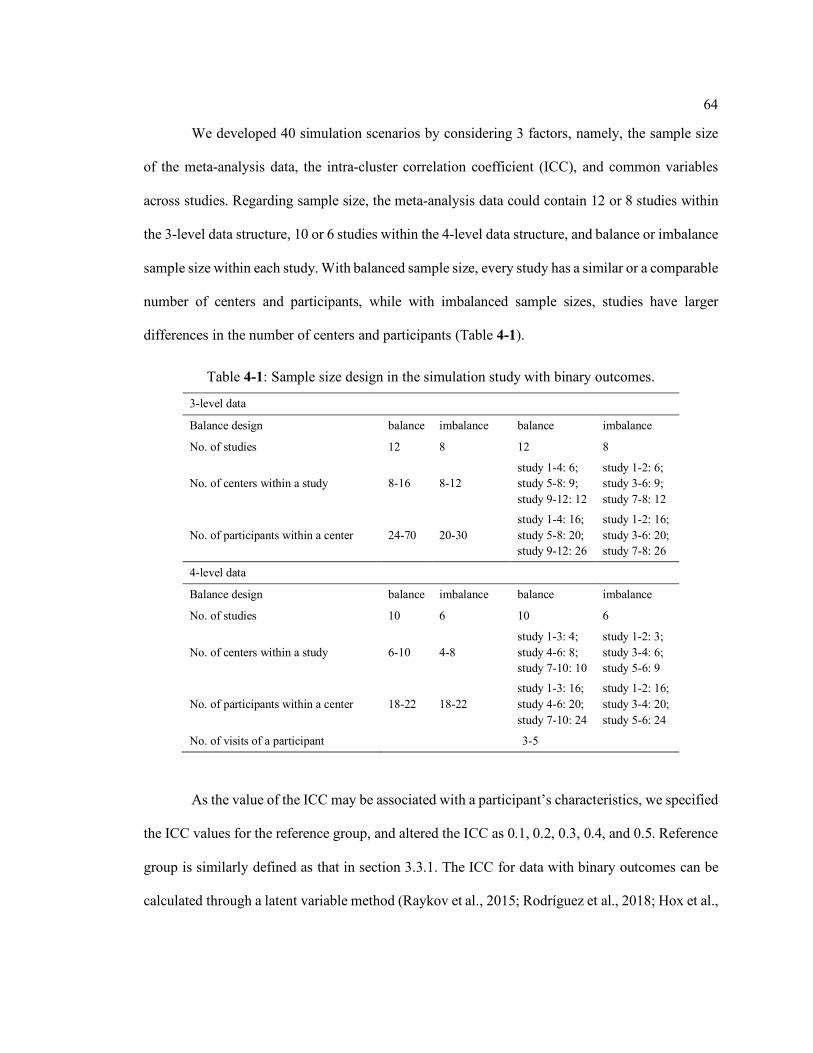
64

We developed 40 simulation scenarios by considering 3 factors, namely, the sample size

of the meta-analysis data, the intra-cluster correlation coefficient (ICC), and common variables

across studies. Regarding sample size, the meta-analysis data could contain 12 or 8 studies within

the 3-level data structure, 10 or 6 studies within the 4-level data structure, and balance or imbalance

sample size within each study. With balanced sample size, every study has a similar or a comparable

number of centers and participants, while with imbalanced sample sizes, studies have larger

differences in the number of centers and participants (Table 4-1).

As the value of the ICC may be associated with a participant’s characteristics, we specified

the ICC values for the reference group, and altered the ICC as 0.1, 0.2, 0.3, 0.4, and 0.5. Reference

group is similarly defined as that in section 3.3.1. The ICC for data with binary outcomes can be

calculated through a latent variable method (Raykov et al., 2015; Rodríguez et al., 2018; Hox et al.,

Table 4-1: Sample size design in the simulation study with binary outcomes.

3-level data







4-level data







No. of visits of a participant 3-5

65

2017). For example, suppose with 3-level data, we have two subjects in the reference group from

the same center of a study, then the ICC equals to

𝐼𝐶𝐶 =

𝜎l__)Líö0 + 𝜎l_Mì�)ìl0

𝜎l__)Líö0 + 𝜎l_Mì�)ìl0 + 𝜋03

where 𝑟_)Líö~𝑁(0, 𝜎l__)Líö0 ) , 𝑟Mì�)ìl~𝑁(0, 𝜎l_Mì�)ìl0 ) , and c´d

represents the within-study

variance when the binary data arise from a logistic distribution with a threshold. In the simulation

study, we specified 𝜎l__)Líö0 : 𝜎l_Mì�)ìl0 = 1: 2. As ICC ranged from 0.1, 0.2 to 0.5, we could decide

the values of 𝜎l__)Líö0 and 𝜎l_Mì�)ìl0 . More details about value specification could be found in the

appendix B.

The covariates collected from each study could be same or different. We considered either

common covariates from each study, or with distinct/unique variables. In scenarios with

distinct/unique variables, we chose gender, race, CVD, and diabetes information as study-specific

variables. In 3-level data, gender was only available in study no. 3 and 5, race was available in

study 1, diabetes was available in study 7, and CVD was available in study 8. With 4-level data,

we only considered gender and race as distinct covariates. We examined each scenario in 1000

simulation runs.

With each simulated dataset, we applied 4 test models to the data (Table 3-2). The models

were a two-stage fixed-effects model, a two-stage random-effects model, a one-stage fixed-effects

model, and a one-stage random-effects (proposed) model. Both two-stage methods still include

center-level and participant-level random effects in the first-stage estimates, whereas the one-stage

fixed-effects model ignores all random effects, and the one-stage proposed model captures all

random effects. To assess the performance of the 4 meta-analytic approaches, we compare the

average of mean estimates, average of standard errors from each simulation, and the coverage

probability of containing the true treatment effect among 1000 simulations.

66

4.3.2 Simulation Results

The mean of the treatment effect (log odds ratios) estimates, the mean of the standard errors

from each estimate, and the coverage probability from 1000 simulations for 3-level and 4-level data

structure with common covariates are shown in Figures 4-1 and 4-2, with different combinations

of sample size and ICC value.

For simulated data with a 3-level structure, the true value of the difference of treatment

effects was specified as -0.8. As seen in Figure 4-1, the two-stage fixed-effects model, the two-

stage random-effects model, and the one-stage proposed model give accurate mean estimates in

most scenarios, ranging from -0.77 to -0.63. As the ICC value increases or with imbalanced design,

the mean estimates become less accurate and more fluctuated. For the one-stage fixed-effects

model, it yields relative larger bias regarding mean estimate in all scenarios comparing with other

three models, especially when ICC increases (mean estimates range from -0.65 to -0.36). As both

fixed-effects models fail to consider appropriate variability in the data, they tend to underestimate

the standard errors when the ICC increases, resulting in poor coverage probabilities. The coverage

probabilities of the two-stage fixed-effects model are less than 0.85. The coverage probabilities of

the one-stage fixed-effects model are always less than 0.75 in all scenarios. The two-stage random-

effects and one-stage proposed models behave similarly on the estimation of variance and coverage

in many scenarios, but when the sample size decreases or becomes imbalanced, the two-stage

random-effects model displays insufficient coverage probability (ranging from 0.823 to 0.893). The

one-stage proposed model is able to appropriately estimate variation between studies and to

maintain about 0.95 coverage probability in all scenarios (ranging from 0.908 to 0.967).

67

Figure 4-1: Simulation results for 3-level data structure with common covariates.

68

For simulations with longitudinal data (4-level structure data) and common covariates

(Figure 4-2), the true value specified for the difference of slopes between groups is -0.4. Both fixed-

effects models show relatively larger bias regarding mean estimate, underestimated variance

estimation, and poor coverage probabilities. The coverage probabilities for both fixed-effects

models are equal or lower than 0.45 in all scenarios. For the two-stage random-effects model and

the one-stage proposed model, similar observations can be made compared with 3-level structure

data. The discrepancy of coverage probabilities between the two models are more apparent

comparing that with 3-level structure data, especially when the ICC value increases, sample size

decreases, or with imbalanced sample size design. The coverage probabilities of the two-stage

random-effects model range from 0.837 to 0.912. The coverage probabilities of the one-stage

proposed model range from 0.937 to 0.955.

Figure 4-2: Simulation results for 4-level data structure with common covariates.

69

Simulation scenarios with distinct covariates display similar observations as that in the data

with common covariates. Results for simulation data with distinct covariates are shown in the

Figures 4-3 to 4-4.

Figure 4-3: Simulation results for 3-level data structure with distinct covariates.

70

4.4 Real Data Application

4.4.1 Example Data - Blood Pressure Studies

We used the same 3 studies from the NHLBI to evaluate the performance of the one-stage

proposed model for exponential family outcomes. The common question we tried to address was

to determine the effect of reducing sodium intake on lowering blood pressure by a certain amount.

The 3 studies are DASH-Sodium, PREMIER, and TOHP (phase II), and the study information and

outcome variables are summarized in Table 4-2.

Figure 4-4: Simulation results for 4-level data structure with distinct covariates.

71

For the purpose of this real data application, we focus on the comparison of the sodium

intake reduction group versus control, advice only, or usual care. DASH-Sodium had a crossover

randomization design, and participants from DASH-Sodium were used as a self-comparison. The

measurement times of the 3 studies were not the same across studies, and we use the closest

measurement times between studies, which were the end of 1 month, 3 months, and 6 months for

DASH-Sodium, PREMIER, and TOHP, respectively. We focused on the change of SBP and the

change of DBP from the baseline to their corresponding selected end time point of each study as

the final outcome variables. For both outcome variables, we considered binary and ordinal outcome

variables. For binary outcomes, we used -10 mmHg and -5 mmHg as the cutoff point for the change

of SBP and the change of DBP, respectively. For the ordinal outcomes, we categorized the change

of SBP as £-10 mmHg, -10 to 0 mm, and >0 mmHg; we categorized the change of DBP as £-5

mmHg, -5 to 0 mmHg, and >0 mmHg.

Table 4-2: Study information summary of the NHLBI studies.

Study DASH-Sodium PREMIER TOHP (phase II)

Study period 1997-2002 1998-2004 1986-1998

Inclusion



SBP <140 mmHg; DBP 83-89 mmHg; free of anti-hypertensive medications

Age range ³22 ³25 30-54

Study design crossover RCT; DASH diet + sodium reduction

parallel RCT; DASH diet + sodium reduction

parallel RCT; weight loss + sodium reduction

Study arms used low vs high (control) sodium level low vs control sodium level low vs control sodium level

Subjects used 204 541 1191

Number of centers 5 4 9

Outcome measure at the end of 1 month at the end of 3 months at the end of 6 months

Binary outcome Change of SBP £-10 mmHg; change of DBP £-5 mmHg

Ordinal outcome Change of SBP: £-10, -10 – 0, >0 mmHg; change of DBP: £-5, -5 – 0 >0 mmHg

SBP: systolic blood pressure; DBP: diastolic blood pressure; RCT: randomized clinical trial.

72

We considered participant-level variables, study-level variables, and random effects

considered, which we included in the one-stage proposed model (Table 4-3). For comparison, we

calculated the individual treatment effects estimated from each study. We also fitted the two-stage

fixed-effects model, the two-stage random-effects model, and the one-stage fixed-effects model to

compare with the one-stage proposed model. We conducted all analyses in SAS 9.4.

4.4.2 Results

For the binary outcomes of SBP and DBP, the individual treatment effect estimates from

each study along with the pooled estimates from the proposed model and other meta-analysis

models are presented in Figures 4-5 to 4-8.

Table 4-3: Model fitting with NHLBI studies.

Covariates DASH-sodium PREMIER TOHP (phase II) Participant-level

Sodium level (low or control) X X X Age X X X Female X X X Race X X X Baseline SBP/DBP X X X Baseline weight X X X Study level

SS_mean X X X SS_std X X X Random effect

Study_treatment X X X Center X X X

SBP: systolic blood pressure; DBP: diastolic blood pressure.

73

For the binary outcome of SBP, all estimates yielded statistically significant results.

Sodium intake reduction had a significant impact on the change of SBP £-10 mmHg. As seen from

the individual estimates from each study, DASH-Sodium (odds ratio (OR)=3.90, 95% CI (2.46,

6.17)) shows the largest OR, followed by TOHP (OR=2.32, 95% CI (1.72, 3.13)) and PREMIER

(OR=2.27, 95% CI (1.57, 3.32)). The overall treatment effect estimate obtained from the one-stage

proposed model was (OR=2.64, 95% CI (1.95, 3.56)). Heterogeneity of the treatment effect existed

between studies, and the one-stage proposed model was able to integrate the information from the

three studies, and gave an appropriate overall estimate. Comparing the estimate from the one-stage

proposed model with other tested models, both two-stage and one-stage fixed-effects models

Figure 4-5: Individual estimates and pooled estimates with the binary SBP outcome.

Figure 4-6: Meta-analysis methods comparison with the binary SBP outcome.

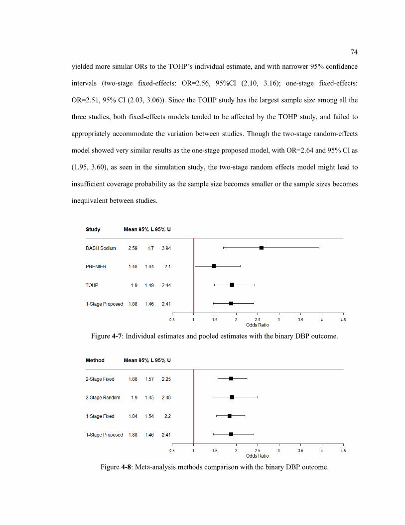
74

yielded more similar ORs to the TOHP’s individual estimate, and with narrower 95% confidence

intervals (two-stage fixed-effects: OR=2.56, 95%CI (2.10, 3.16); one-stage fixed-effects:

OR=2.51, 95% CI (2.03, 3.06)). Since the TOHP study has the largest sample size among all the

three studies, both fixed-effects models tended to be affected by the TOHP study, and failed to

appropriately accommodate the variation between studies. Though the two-stage random-effects

model showed very similar results as the one-stage proposed model, with OR=2.64 and 95% CI as

(1.95, 3.60), as seen in the simulation study, the two-stage random effects model might lead to

insufficient coverage probability as the sample size becomes smaller or the sample sizes becomes

inequivalent between studies.

Figure 4-7: Individual estimates and pooled estimates with the binary DBP outcome.

Figure 4-8: Meta-analysis methods comparison with the binary DBP outcome.

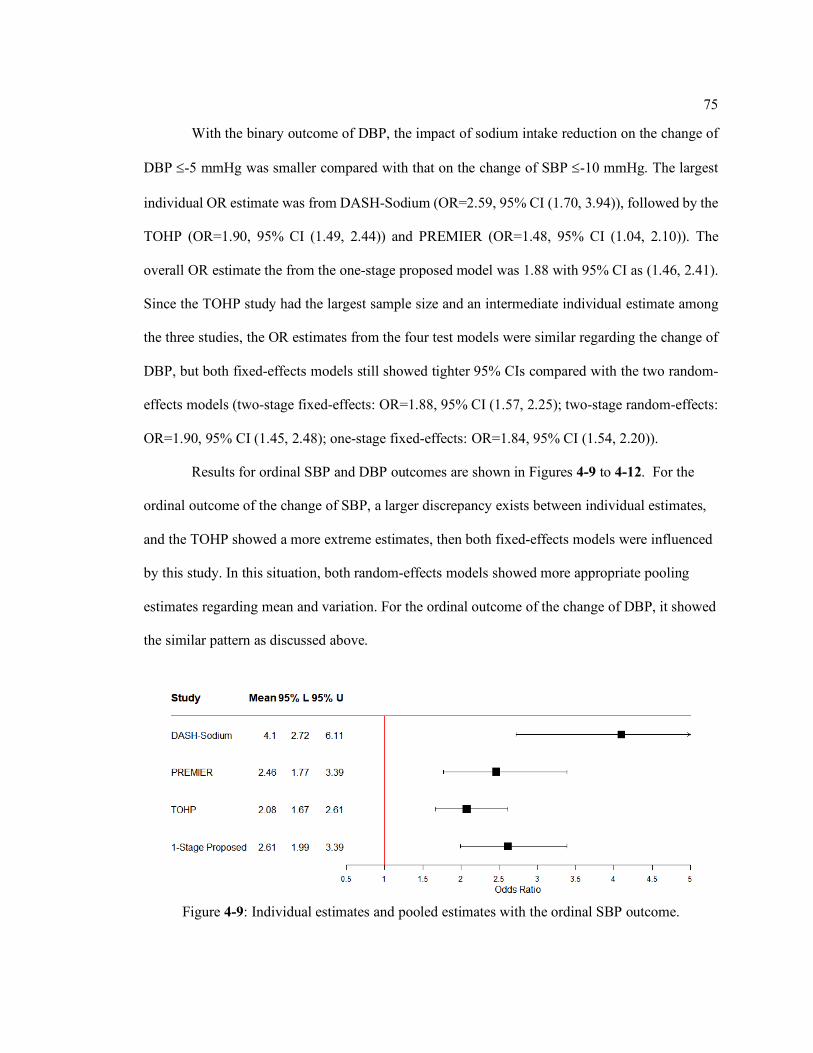
75

With the binary outcome of DBP, the impact of sodium intake reduction on the change of

DBP £-5 mmHg was smaller compared with that on the change of SBP £-10 mmHg. The largest

individual OR estimate was from DASH-Sodium (OR=2.59, 95% CI (1.70, 3.94)), followed by the

TOHP (OR=1.90, 95% CI (1.49, 2.44)) and PREMIER (OR=1.48, 95% CI (1.04, 2.10)). The

overall OR estimate the from the one-stage proposed model was 1.88 with 95% CI as (1.46, 2.41).

Since the TOHP study had the largest sample size and an intermediate individual estimate among

the three studies, the OR estimates from the four test models were similar regarding the change of

DBP, but both fixed-effects models still showed tighter 95% CIs compared with the two random-

effects models (two-stage fixed-effects: OR=1.88, 95% CI (1.57, 2.25); two-stage random-effects:

OR=1.90, 95% CI (1.45, 2.48); one-stage fixed-effects: OR=1.84, 95% CI (1.54, 2.20)).

Results for ordinal SBP and DBP outcomes are shown in Figures 4-9 to 4-12. For the

ordinal outcome of the change of SBP, a larger discrepancy exists between individual estimates,

and the TOHP showed a more extreme estimates, then both fixed-effects models were influenced

by this study. In this situation, both random-effects models showed more appropriate pooling

estimates regarding mean and variation. For the ordinal outcome of the change of DBP, it showed

the similar pattern as discussed above.

Figure 4-9: Individual estimates and pooled estimates with the ordinal SBP outcome.

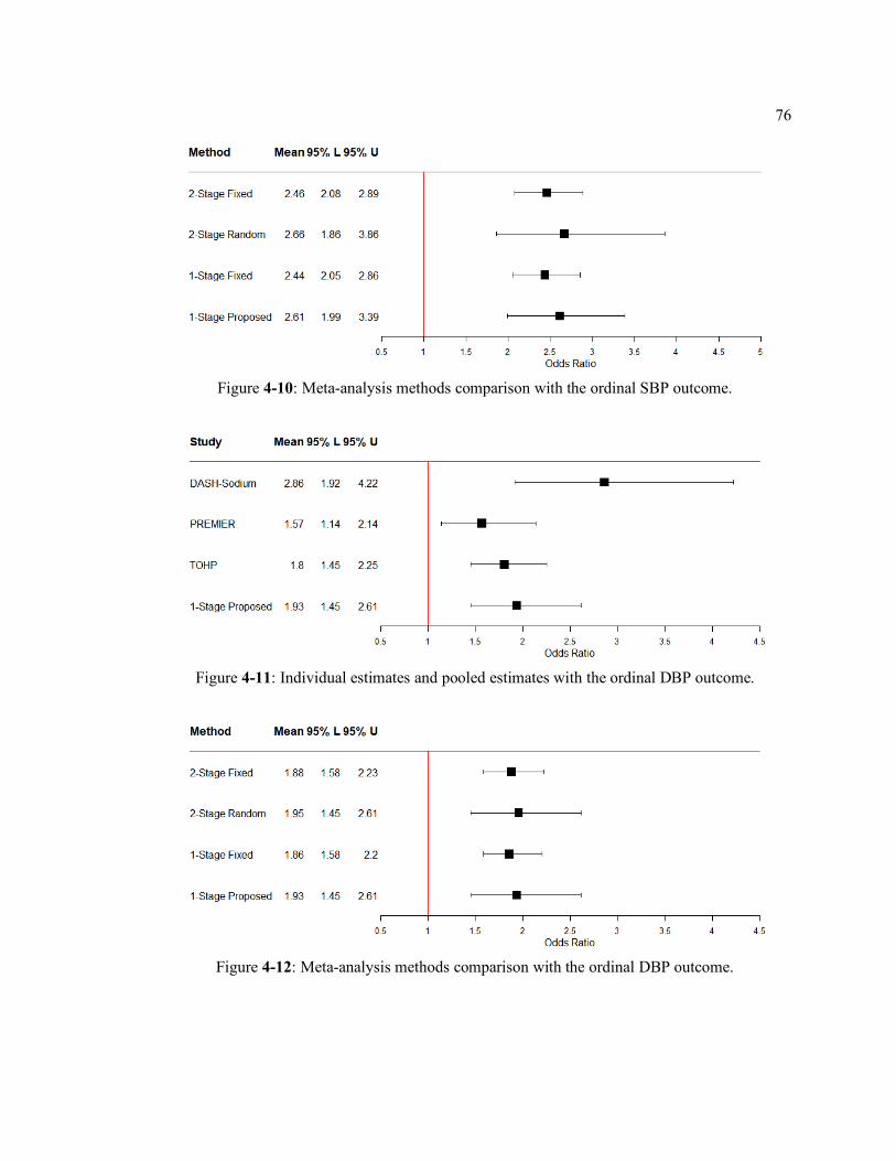
76

Figure 4-10: Meta-analysis methods comparison with the ordinal SBP outcome.

Figure 4-11: Individual estimates and pooled estimates with the ordinal DBP outcome.

Figure 4-12: Meta-analysis methods comparison with the ordinal DBP outcome.

77

Chapter 5

Summary and Future Work

We propose a one-stage multi-level mixed-effect model for IPD meta-analysis which

logically incorporates the hierarchy structure of meta-analysis data, maximally utilizes the

information from each study, and provides more flexibility to address different research questions.

The proposed model is firstly developed for data with a continuous outcome in chapter 3, and then

extended to outcomes from an exponential family in chapter 4. Besides continuous outcomes,

binary, categorical or count outcomes also are very common in practical research, and the extension

of application from continuous outcomes to exponential family outcomes greatly improve the

application range.

One-stage IPD meta-analysis methods are based on exact modeling of the likelihood

function, and thus avoid the biases that can arise in two-stage methods. Allowing both fixed effects

and random effects at each level helps in identifying different sources of variation. The proposed

model is applicable to either observational studies or randomized studies with or without repeated

measurements. In both simulation studies, we investigated 40 simulation scenarios, respectively,

including three different factors, different sample sizes, different ICC values, and whether studies

have common or distinct covariates. The four tested models presented small biases regarding the

mean estimate in most scenarios when we specified the treatment effects of each study came from

a same normal distribution. In practice, however, it is likely that treatment effects from each study

do not share the same distribution, which would be more complicated to test in a simulation study.

Nonetheless, we still clearly could notice the different abilities of appropriately estimating the

variation between methods. Both fixed-effects models fail to correctly capture the variability in the

data, and result in poorer coverage probabilities, especially when the between-study variance

78

increases. The one-stage fixed-effects model performs worst as it totally ignores any random effects

in the model. The two-stage random-effects model though displays similar mean and variance

estimates compared with the one-stage proposed model in most cases, the one-stage proposed

model is always able to provide about 0.95 coverage probability in most cases, especially when

sample size decreases, sample size become imbalanced between studies, or the ICC value increases.

In the real data applications, large or smaller amounts of heterogeneity of the effect size existed

across studies, and the one-stage proposed model reasonably accounts for the heterogeneity

compared with both of the fixed-effects models. Though little difference was observed between the

two-stage random-effects model and the one-stage proposed model, as shown through the

simulation study, more apparent differences on coverage probability between the two models was

observed, especially when the ICC increased. Through both simulation studies and the real data

examples, fixed-effects models showed certain limitations and problems. They tended to

underestimate the variation of the meta-analytic data, and their results are usually dominated by the

studies with larger scale.

Though the one-stage proposed model has complex specifications, it still has the form of a

LMM or GLMM. Thus, the implementation of the model is straightforward and is usually available

in primary programming languages. Since the solution is based on maximizing the likelihood

function by literately updating the parameters until convergence, it usually is more computationally

demanding than two-stage methods, and it may encounter a convergence problem on occasion. In

the main simulation studies conducted, we did not encounter convergence issues with the 3-level

structure data, and only experienced about 5% of the simulated data sets that failed to converge

with the 4-level structure data. In chapter 4, the calculation involves the approximation to the

integration of random effects, and we used PQL to approximate the integration of random effects,

since quasi-likelihood methods usually have a higher chance and a faster speed to achieve the

approximation. Also, other researchers have shown that, for binary data with relatively small

79

number of repeated measurements, PQL may result in substantial bias as the accuracy depends on

the distribution assumption of the pseudo-data. Other techniques mentioned previously are also

recommended if the quasi-likelihood method fails. The inclusion of random effects needs to be

done cautiously. Inappropriately incorporating redundant random effects may lead to misleading

results and convergence failure as the number of parameters increases or the variance components

are non-identifiable. For example, if there are only limited eligible studies, the inclusion of study-

level random effects should be restricted. Sufficient explorations, such as graphical techniques,

should be conducted before adding random effects to the model. Including more random effects

may also lead to an identifiability problem when estimating variance-covariance parameters. The

identifiability problem indicates that the sources of variation cannot be correctly differentiated, and

results in incorrect variance-covariance estimates.

Another consideration is about the selection of covariates. The selection of covariates from

each study should also follow major variable selection principles. Covariates included should be

associated with the outcome variable no matter statistically or scientifically. The form of the

variable included in the model should be evaluated. The model can be applied to longitudinal data,

but in practice, the measurement time points may or may not be the same across studies. If the

lengths of follow-up time and time points are very different from each other, it may not be

appropriate to simply pool studies together, as the slopes of each study are actually different

between studies, and it is not proper to pool them together. Selecting time points within a similar

follow-up time period for each study is recommended.

Bayesian methods have been investigated to develop the method for meta-analysis. When

applying Bayesian methods, the prior distributions for effect size and between-study variance need

to be decided. A previous study already shows the pooled effect size is sensitive the choice to or

prior distribution for the between-study variance, even with different noninformative or vague

priors (Lambert et al., 2005). Other researchers have tried to utilize existing meta-analysis results

80

to generate the informative empirical priors for unknown parameters for both continuous and binary

outcomes (Riley et al., 2008; Rhodes et al., 2014; Turner et al., 2012). Bayesian meta-analysis

methods have been extended to bivariate or multivariate meta-analysis. It has been suggested that

vague priors should be avoided through simulation studies, and sensible or empirical priors are

recommended (Burke et al., 2016). Bayesian methods have also been developed for meta-analysis

with mixed types of outcomes, such as continuous and binary, which are usually based on a two-

stage method framework (Bujkiewicz et al., 2013; Wei et al., 2013, Riley et al., 2015).

In summary, the proposed model can be applied to IPD meta-analysis data with cross-

sectional data or longitudinal data, with continuous or exponential family outcomes, which attempts

to maximally utilize the information and hierarchy feature of the data. The model could be

evaluated in more aspects, such as more extreme sample size settings, other type of outcomes from

an exponential family, the impact of different integration approximation methods. Besides

continuous outcomes and outcomes from an exponential family, time-to-event outcomes are also

very common in biomedical research, so the extension of the proposed model to survival outcome

is necessary.

81

Appendix A

Chapter 3

A.1 Simulation Study

/*** 3-level Data Simulation ***/ /*** Generate data ***/ proc format; value treat 0='Placebo' 1='Active'; value ny 0='No' 1='Yes'; value race 1='Caucasian' 2='African American' 3='Hispanic' 4='Other'; run; /*ICC=0.1 vs=6.25 vc=18.75 v=225 vs_trt=vs/2 vc_bc=vc/2*/ /*ICC=0.2 vs=14.0625 vc=42.1875 v=225 vs_trt=vs/2 vc_bc=vc/2*/ /*ICC=0.3 vs=32.14286 vc=64.28571 v=225 vs_trt=vs/2 vc_bc=vc/2*/ /*ICC=0.4 vs=50 vc=100 v=225 vs_trt=vs/2 vc_bc=vc/2*/ /*ICC=0.5 vs=75 vc=150 v=225 vs_trt=vs/2 vc_bc=vc/2*/ %macro simulation(n); %do sample=1 %to 4; %do icc=1 %to 5; %do common=1 %to 1; %do i=1 %to &n.; /*Participant-level covariates + study-level var*/ data simulated_data; sample=&sample.; icc=&icc.; common=&common.; if sample in (1,3) then num_studies=12; else num_studies=8; intercept=220; beta_treatment=-8; beta_basecholesterol=0.2; beta_age=0.2; beta_female=-4; beta_female_3=-3; beta_female_5=-4; beta_AfrAm=4; beta_Hisp=6; beta_Other=-0.8; beta_diabetes=6; beta_CVD=6; beta_ss_mean=-0.3; beta_ss_std=1.5;

82

beta_order=-0.5; do study=1 to num_studies by 1; if sample=1 then num_centers=round(8+(8*rand('uniform'))); *range: 8-16; else if sample=2 then num_centers=round(8+(4*rand('uniform'))); *range: 8-12; else if sample=3 then num_centers=(study<5)*6+(study>=5)*(study<9)*9+(study>=9)*12; else num_centers=(study<3)*6+(study>=3)*(study<7)*9+(study>=7)*12; order=study; *sequential order of the study = study #; if icc=1 then do; r1=rand('normal',0,sqrt(6.25)); *study-level random intercept; r1_trt=rand('normal',0,sqrt(6.25/2)); *study-level random trt effect; end; else if icc=2 then do; r1=rand('normal',0,sqrt(14.0625)); *study-level random intercept; r1_trt=rand('normal',0,sqrt(14.0625/2)); *study-level random trt effect; end; else if icc=3 then do; r1=rand('normal',0,sqrt(32.14286)); *study-level random intercept; r1_trt=rand('normal',0,sqrt(32.14286/2)); *study-level random trt effect; end; else if icc=4 then do; r1=rand('normal',0,sqrt(50)); *study-level random intercept; r1_trt=rand('normal',0,sqrt(50/2)); *study-level random trt effect; end; else do; r1=rand('normal',0,sqrt(75)); *study-level random intercept; r1_trt=rand('normal',0,sqrt(75/2)); *study-level random trt effect; end; do center=1 to num_centers by 1; if sample=1 then sample_size=round(24+(46*rand('uniform'))); *range: 24-70; else if sample=2 then sample_size=round(20+(10*rand('uniform'))); *range: 20-30;

83

else if sample=3 then sample_size=(study<5)*16+(study>=5)*(study<9)*20+(study>=9)*26; else sample_size=(study<3)*16+(study>=3)*(study<7)*20+(study>=7)*26; if mod(sample_size,2)=1 then sample_size=sample_size+1; *guarantee equal sizes for two arms; if icc=1 then do; r2=rand('normal',0,sqrt(18.75)); r2_bc=rand('normal',0,sqrt(18.75/2)); end; else if icc=2 then do; r2=rand('normal',0,sqrt(42.1875)); r2_bc=rand('normal',0,sqrt(42.1875/2)); end; else if icc=3 then do; r2=rand('normal',0,sqrt(64.28571)); r2_bc=rand('normal',0,sqrt(64.28571/2)); end; else if icc=4 then do; r2=rand('normal',0,sqrt(100)); r2_bc=rand('normal',0,sqrt(100/2)); end; else do; r2=rand('normal',0,sqrt(150)); r2_bc=rand('normal',0,sqrt(150/2)); end; do participant=1 to sample_size by 1; if (participant<=sample_size/2) then treatment=0; else treatment=1; age=round(rand('normal',50,8)); basecholesterol=round(rand('normal',240,3)); if common=1 then do; rand_female=rand('uniform'); if (0.00<=rand_female<0.60) then female=0; if (0.60<=rand_female) then female=1; rand_race=rand('uniform'); if (0.00<=rand_race<0.50) then race=1; if (0.50<=rand_race<0.70) then race=2; if (0.70<=rand_race<0.90) then race=3; if (0.90<=rand_race) then race=4; rand_diabetes=rand('uniform');

84

if (0.00<=rand_diabetes<0.60) then diabetes=0; if (0.60<=rand_diabetes) then diabetes=1; rand_CVD=rand('uniform'); if (0.00<=rand_CVD<0.70) then CVD=0; if (0.70<=rand_CVD) then CVD=1; end; else do; female=0; rand_female=rand('uniform'); if (0.00<=rand_female<0.60 and study in (3,5)) then female=0; if (0.60<=rand_female and study in (3,5)) then female=1; race=0; rand_race=rand('uniform'); if (0.00<=rand_race<0.50 and study=1) then race=1; if (0.50<=rand_race<0.70 and study=1) then race=2; if (0.70<=rand_race<0.90 and study=1) then race=3; if (0.90<=rand_race and study=1) then race=4; diabetes=0; rand_diabetes=rand('uniform'); if (0.00<=rand_diabetes<0.60 and study=7) then diabetes=0; if (0.60<=rand_diabetes and study=7) then diabetes=1; CVD=0; rand_CVD=rand('uniform'); if (0.00<=rand_CVD<0.70 and study=8) then CVD=0; if (0.70<=rand_CVD and study=8) then CVD=1; end; format treatment treat. female ny. race race. diabetes CVD ny.; output; end; end; end; run; /*Study-level variables: ss_mean ss_std*/ proc sort data=simulated_data out=sort (keep=study num_centers center sample_size) nodupkey; by study center; run; proc means data=sort mean var noprint; var sample_size; class study;

85

output out=mean_var mean=ss_mean std=ss_std; run; data simulated_data2; merge simulated_data mean_var; by study; if study=. then delete; drop _type_ _freq_; run; /*Generate outcome variable: serum_cholesterol*/ proc sql noprint; select mean(basecholesterol),mean(age) into :mean_bc, :mean_age from simulated_data2; quit; data simulated_data2; set simulated_data2; cntr_bc=basecholesterol-&mean_bc.; cntr_age=age-&mean_age.; if common=1 then do; mean=intercept+(cntr_bc*beta_basecholesterol)+(treatment*beta_treatment)+(cntr_age*beta_age)+(female*beta_female) +((race=2)*beta_AfrAm)+((race=3)*beta_Hisp)+((race=4)*beta_Other)+(diabetes*beta_diabetes)+(CVD*beta_CVD) +(ss_mean*beta_ss_mean)+(ss_std*beta_ss_std)+(order*beta_order) +r1+(treatment*r1_trt)+r2+(cntr_bc*r2_bc); end; else do; mean=intercept+(cntr_bc*beta_basecholesterol)+(treatment*beta_treatment)+(cntr_age*beta_age) +((study=3)*female*beta_female_3)+((study=5)*female*beta_female_5) +((study=1)*(race=2)*beta_AfrAm)+((study=1)*(race=3)*beta_Hisp)+((study=1)*(race=4)*beta_Other) +((study=7)*diabetes*beta_diabetes)+((study=8)*CVD*beta_CVD) +(ss_mean*beta_ss_mean)+(ss_std*beta_ss_std)+(order*beta_order) +r1+(treatment*r1_trt)+r2+(cntr_bc*r2_bc); end; serum_cholesterol=round(rand('normal',mean,15)); run; /*two-stage methods*/ %if &sample.=1 or &sample.=3 %then %do; %let nums=12; %end; %else %do; %let nums=8; %end;

86

%do s=1 %to &nums.; data dat&s.; set simulated_data2; if study=&s.; run; proc mixed data=dat&s. covtest; class treatment center; model serum_cholesterol=treatment cntr_bc cntr_age female race diabetes CVD /solution; random intercept cntr_bc/ type=vc subject=center; ods exclude all; ods output SolutionF=S&s.; run; data NS&s.; studyno=&s.; set S&s.; if treatment=1; est=StdErr**2; keep studyno Estimate EST; run; %if &s.=1 %then %do; data trt; set NS&s.; run; %end; %else %do; proc append base=trt data=NS&s.; run; %end; %end; /*Fixed-effects model*/ data trt; set trt; w=1/est; wy=w*Estimate; run; data out_temp; stop; run; proc sql; create table out_temp as select sum(wy)/sum(w) as treatment_overall, sqrt(1/sum(w)) as se from trt; quit; data out_temp; no=&i.;

87

set out_temp; lower=treatment_overall-1.96*se; upper=treatment_overall+1.96*se; run; %if &i.=1 %then %do; data d.fixed_s&sample.i&icc.c&common.; set out_temp; run; %end; %else %do; proc append base=d.fixed_s&sample.i&icc.c&common. data=out_temp; run; %end; /*Random-effects model*/ data trt; set trt; wy2=w*estimate**2; w2=w**2; run; proc sql; select ((sum(wy2)-sum(wy)**2/sum(w))-(&nums.-1))/(sum(w)-sum(w**2)/sum(w)) into: b_var from trt; quit; data trt; set trt; w_r=1/(est+&b_var.); wy_2=w_r*Estimate; run; data out_temp; stop; run; proc sql; create table out_temp as select sum(wy_2)/sum(w_r) as treatment_overall, sqrt(1/sum(w_r)) as se from trt; quit; data out_temp; no=&i.; set out_temp; lower=treatment_overall-1.96*se; upper=treatment_overall+1.96*se; between_trt=&b_var.; run; %if &i.=1 %then %do; data d.random_s&sample.i&icc.c&common.; set out_temp;

88

run; %end; %else %do; proc append base=d.random_s&sample.i&icc.c&common. data=out_temp; run; %end; /*** LMM ***/ /*** 3-level models ***/ %if &common.=1 %then %do; /*Proposed model*/ title 'Full model'; proc mixed data=simulated_data2 covtest; class female(ref='No') race(ref='Caucasian') diabetes(ref='No') CVD(ref='No') center study; model serum_cholesterol=treatment cntr_bc cntr_age female race diabetes CVD ss_mean ss_std order/solution cl; random intercept cntr_bc/ type=vc subject=center(study); random intercept treatment/ type=vc subject=study; ods exclude all; ods output SolutionF=SolutionF1; ods output CovParms=CovParms1; run; %out(SolutionF=SolutionF1,CovParms=CovParms1,num=1,sample=&sample.,icc=&icc.,common=&common.); /*Model 1*/ title 'Model 1'; proc mixed data=simulated_data2 covtest; class female(ref='No') race(ref='Caucasian') diabetes(ref='No') CVD(ref='No') center study; model serum_cholesterol=treatment cntr_bc cntr_age female race diabetes CVD /solution cl; ods exclude all; ods output SolutionF=SolutionF2; ods output CovParms=CovParms2; run; %out(SolutionF=SolutionF2,CovParms=CovParms2,num=2,sample=&sample.,icc=&icc.,common=&common.); %end; %else %do; /*** LMM ***/ /*** unique 3-level models ***/ data simulated_data2; set simulated_data2; AfrAm=0;Hisp=0;Other=0; if race=2 then AfrAm=1; if race=3 then Hisp=1; if race=4 then Other=1;

89

run; /*Proposed model*/ title 'Full model'; proc mixed data=simulated_data2 covtest; class center study; model serum_cholesterol=treatment cntr_bc cntr_age female(study) AfrAm(study) Hisp(study) Other(study) diabetes(study) CVD(study) ss_mean ss_std order/solution cl; random intercept cntr_bc/ type=vc subject=center(study); random intercept treatment/ type=vc subject=study ; ods exclude all; ods output SolutionF=SolutionF1; ods output CovParms=CovParms1; run; %out(SolutionF=SolutionF1,CovParms=CovParms1,num=1,sample=&sample.,icc=&icc.,common=&common.); /*Model 1*/ title 'Model 1'; proc mixed data=simulated_data2 covtest; class center study; model serum_cholesterol=treatment cntr_bc cntr_age female(study) AfrAm(study) Hisp(study) Other(study) diabetes(study) CVD(study) /solution cl; ods exclude all; ods output SolutionF=SolutionF2; ods output CovParms=CovParms2; run; %out(SolutionF=SolutionF2,CovParms=CovParms2,num=2,sample=&sample.,icc=&icc.,common=&common.); %end; %end; %end; %end; %end; %mend simulation; %simulation(n=1000); /*** 4-level Data Simulation ***/ /*** Generate data ***/ proc format; value treat 0='Placebo' 1='Active'; value ny 0='No' 1='Yes'; value race 1='Caucasian' 2='African American' 3='Hispanic' 4='Other';

90

run; /*ICC=0.1 vs=4.166667 vc=8.333333 vp=12.5 v=225 vs_trt=vs/2 */ /*ICC=0.2 vs=9.375 vc=18.75 vp=28.125 v=225 vs_trt=vs/2 */ /*ICC=0.3 vs=16.071429 vc=32.142857 vp=48.21429 v=225 vs_trt=vs/2 */ /*ICC=0.4 vs=25 vc=50 vp=75 v=225 vs_trt=vs/2 */ /*ICC=0.5 vs=37.5 vc=75 vp=112.5 v=225 vs_trt=vs/2 */ %macro simulation(n); %do sample=1 %to 4; %do icc=1 %to 5; %do common=1 %to 2; %do i=1 %to &n.; /*Participant-level covariates + study-level var*/ data simulated_data; sample=&sample.; icc=&icc.; common=&common.; if sample in (1,3) then num_studies=10; else num_studies=6; intercept=220; beta_basecholesterol=0.2; beta_age=0.2; beta_female=-4; beta_female_3=-3; beta_female_5=-4; beta_AfrAm=4; beta_Hisp=6; beta_Other=-0.8; beta_diabetes=6; beta_CVD=6; beta_ss_mean=-0.3; beta_ss_std=1.5; beta_order=-0.5; beta_weight=0.4; beta_visit=-1; beta_visit_trt=-4; do study=1 to num_studies by 1; if sample=1 then num_centers=round(6+(4*rand('uniform'))); *range: 6-10; else if sample=2 then num_centers=round(4+(4*rand('uniform'))); *range: 4-8; else if sample=3 then num_centers=(study<4)*4+(study>=4)*(study<7)*8+(study>=7)*12; else num_centers=(study<3)*3+(study>=3)*(study<5)*6+(study>=5)*9; order=study; *sequential order of the study = study #;

91

if icc=1 then do; r1=rand('normal',0,sqrt(4.166667)); *study-level random intercept; r1_trt=rand('normal',0,sqrt(4.166667/2)); *study-level random trt effect; end; else if icc=2 then do; r1=rand('normal',0,sqrt(9.375)); *study-level random intercept; r1_trt=rand('normal',0,sqrt(9.375/2)); *study-level random trt effect; end; else if icc=3 then do; r1=rand('normal',0,sqrt(16.071429)); *study-level random intercept; r1_trt=rand('normal',0,sqrt(16.071429/2)); *study-level random trt effect; end; else if icc=4 then do; r1=rand('normal',0,sqrt(25)); *study-level random intercept; r1_trt=rand('normal',0,sqrt(25/2)); *study-level random trt effect; end; else do; r1=rand('normal',0,sqrt(37.5)); *study-level random intercept; r1_trt=rand('normal',0,sqrt(37.5/2)); *study-level random trt effect; end; do center=1 to num_centers by 1; if sample=1 then sample_size=round(24+(46*rand('uniform'))); *range: 24-70; else if sample=2 then sample_size=round(20+(10*rand('uniform'))); *range: 20-30; else if sample=3 then sample_size=(study<5)*16+(study>=5)*(study<9)*20+(study>=9)*26; else sample_size=(study<3)*16+(study>=3)*(study<7)*20+(study>=7)*26; if mod(sample_size,2)=1 then sample_size=sample_size+1; *guarantee equal sizes for two arms; if icc=1 then do; r2=rand('normal',0,sqrt(8.333333)); end; else if icc=2 then

92

do; r2=rand('normal',0,sqrt(18.75)); end; else if icc=3 then do; r2=rand('normal',0,sqrt(32.142857)); end; else if icc=4 then do; r2=rand('normal',0,sqrt(50)); end; else do; r2=rand('normal',0,sqrt(75)); end; do participant=1 to sample_size by 1; rand_visit=rand('uniform'); if (0.00<=rand_visit<0.80) then visit_num=5; if (0.80<=rand_visit<0.95) then visit_num=4; if (0.95<=rand_visit) then visit_num=3; *range: 3-5; if (participant<=sample_size/2) then treatment=0; else treatment=1; age=round(rand('normal',50,8)); basecholesterol=round(rand('normal',240,3)); if common=1 then do; rand_female=rand('uniform'); if (0.00<=rand_female<0.60) then female=0; if (0.60<=rand_female) then female=1; rand_race=rand('uniform'); if (0.00<=rand_race<0.50) then race=1; if (0.50<=rand_race<0.70) then race=2; if (0.70<=rand_race<0.90) then race=3; if (0.90<=rand_race) then race=4; rand_diabetes=rand('uniform'); if (0.00<=rand_diabetes<0.60) then diabetes=0; if (0.60<=rand_diabetes) then diabetes=1; rand_CVD=rand('uniform'); if (0.00<=rand_CVD<0.70) then CVD=0; if (0.70<=rand_CVD) then CVD=1; end; else do; female=0; rand_female=rand('uniform'); if (0.00<=rand_female<0.60 and study in (3,5)) then female=0;

93

if (0.60<=rand_female and study in (3,5)) then female=1; race=0; rand_race=rand('uniform'); if (0.00<=rand_race<0.50 and study=1) then race=1; if (0.50<=rand_race<0.70 and study=1) then race=2; if (0.70<=rand_race<0.90 and study=1) then race=3; if (0.90<=rand_race and study=1) then race=4; diabetes=0; rand_diabetes=rand('uniform'); if (0.00<=rand_diabetes<0.60 and study=7) then diabetes=0; if (0.60<=rand_diabetes and study=7) then diabetes=1; CVD=0; rand_CVD=rand('uniform'); if (0.00<=rand_CVD<0.70 and study=8) then CVD=0; if (0.70<=rand_CVD and study=8) then CVD=1; end; if icc=1 then do; r3=rand('normal',0,sqrt(12.5)); end; else if icc=2 then do; r3=rand('normal',0,sqrt(28.125)); end; else if icc=3 then do; r3=rand('normal',0,sqrt(48.21429)); end; else if icc=4 then do; r3=rand('normal',0,sqrt(75)); end; else do; r3=rand('normal',0,sqrt(112.5)); end; do visit=1 to visit_num by 1; if treatment=0 then weight=round(rand('normal',150,3)); else weight=round(rand('normal',150-visit*1.5,3)); output; end; format treatment treat. female ny. race race. diabetes CVD ny.; output; end;

94

end; end; run; /*Study-level variables: ss_mean ss_std*/ proc sort data=simulated_data out=sort (keep=study num_centers center sample_size) nodupkey; by study center; run; proc means data=sort mean var noprint; var sample_size; class study; output out=mean_var mean=ss_mean std=ss_std; run; data simulated_data2; merge simulated_data mean_var; by study; if study=. then delete; drop _type_ _freq_; run; /*Generate outcome variable: serum_cholesterol*/ proc sql noprint; select mean(basecholesterol),mean(age),mean(weight) into :mean_bc, :mean_age, :mean_weight from simulated_data2; quit; data simulated_data2; set simulated_data2; cntr_bc=basecholesterol-&mean_bc.; cntr_age=age-&mean_age.; cntr_weight=weight-&mean_weight.; if common=1 then do; mean=intercept+(cntr_bc*beta_basecholesterol)+(cntr_age*beta_age)+(female*beta_female) +((race=2)*beta_AfrAm)+((race=3)*beta_Hisp)+((race=4)*beta_Other)+(diabetes*beta_diabetes)+(CVD*beta_CVD) +(ss_mean*beta_ss_mean)+(ss_std*beta_ss_std)+(order*beta_order) +(cntr_weight*beta_weight)+(visit*beta_visit)+(visit*treatment*beta_visit_trt) +r1+(visit*treatment*r1_trt)+r2+r3; end; else do; mean=intercept+(cntr_bc*beta_basecholesterol)+(cntr_age*beta_age) +((study=3)*female*beta_female_3)+((study=5)*female*beta_female_5) +((study=1)*(race=2)*beta_AfrAm)+((study=1)*(race=3)*beta_Hisp)+((study=1)*(race=4)*beta_Other) +((study=7)*diabetes*beta_diabetes)+((study=8)*CVD*beta_CVD) +(ss_mean*beta_ss_mean)+(ss_std*beta_ss_std)+(order*beta_order)

95

+(cntr_weight*beta_weight)+(visit*beta_visit)+(visit*treatment*beta_visit_trt) +r1+(visit*treatment*r1_trt)+r2+r3; end; serum_cholesterol=round(rand('normal',mean,15)); run; /*two-stage methods*/ %if &sample.=1 or &sample.=3 %then %do; %let nums=10; %end; %else %do; %let nums=6; %end; %do s=1 %to &nums.; data dat&s.; set simulated_data2; if study=&s.; run; proc mixed data=dat&s. covtest; class treatment center participant; model serum_cholesterol=cntr_bc cntr_age female race diabetes CVD cntr_weight visit visit*treatment/solution; random intercept/ type=vc subject=participant(center); random intercept/ type=vc subject=center; ods exclude all; ods output SolutionF=S&s.; run; data NS&s.; studyno=&s.; set S&s.; if treatment=1; est=StdErr**2; keep studyno Estimate EST; run; %if &s.=1 %then %do; data trt; set NS&s.; run; %end; %else %do; proc append base=trt data=NS&s.; run; %end; %end;

96

/*Fixed-effects model*/ data trt; set trt; w=1/est; wy=w*Estimate; run; data out_temp; stop; run; proc sql; create table out_temp as select sum(wy)/sum(w) as treatment_overall, sqrt(1/sum(w)) as se from trt; quit; data out_temp; no=&i.; set out_temp; lower=treatment_overall-1.96*se; upper=treatment_overall+1.96*se; run; %if &i.=1 %then %do; data d.fixed_s&sample.i&icc.c&common.; set out_temp; run; %end; %else %do; proc append base=d.fixed_s&sample.i&icc.c&common. data=out_temp; run; %end; /*Random-effects model*/ data trt; set trt; wy2=w*estimate**2; w2=w**2; run; proc sql; select ((sum(wy2)-sum(wy)**2/sum(w))-(&nums.-1))/(sum(w)-sum(w**2)/sum(w)) into: b_var from trt; quit; data trt; set trt; w_r=1/(est+&b_var.); wy_2=w_r*Estimate; run; data out_temp; stop; run;

97

proc sql; create table out_temp as select sum(wy_2)/sum(w_r) as treatment_overall, sqrt(1/sum(w_r)) as se from trt; quit; data out_temp; no=&i.; set out_temp; lower=treatment_overall-1.96*se; upper=treatment_overall+1.96*se; between_trt=&b_var.; run; %if &i.=1 %then %do; data d.random_s&sample.i&icc.c&common.; set out_temp; run; %end; %else %do; proc append base=d.random_s&sample.i&icc.c&common. data=out_temp; run; %end; /*** LMM ***/ /*** 4-level models ***/ %if &common.=1 %then %do; /*Proposed model*/ title 'Full model'; proc mixed data=simulated_data2 covtest; class female(ref='No') race(ref='Caucasian') diabetes(ref='No') CVD(ref='No') treatment participant center study; model serum_cholesterol=cntr_bc cntr_age female race diabetes CVD ss_mean ss_std order cntr_weight visit visit*treatment/solution cl; random intercept / type=vc subject=participant(center study); random intercept / type=vc subject=center(study); random intercept visit*treatment/ type=vc subject=study; ods exclude all; ods output SolutionF=SolutionF1; ods output CovParms=CovParms1; run; %out(SolutionF=SolutionF1,CovParms=CovParms1,num=1,sample=&sample.,icc=&icc.,common=&common.); /*Model 1*/ title 'Model 1'; proc mixed data=simulated_data2 covtest;

98

class female(ref='No') race(ref='Caucasian') diabetes(ref='No') CVD(ref='No') treatment participant center study; model serum_cholesterol=cntr_bc cntr_age female race diabetes CVD cntr_weight visit visit*treatment/solution cl; repeated / type=vc subject=participant(center study); ods exclude all; ods output SolutionF=SolutionF2; ods output CovParms=CovParms2; run; %out(SolutionF=SolutionF2,CovParms=CovParms2,num=2,sample=&sample.,icc=&icc.,common=&common.); %end; %else %do; /*** LMM ***/ /*** unique 3-level models ***/ data simulated_data2; set simulated_data2; AfrAm=0;Hisp=0;Other=0; if race=2 then AfrAm=1; if race=3 then Hisp=1; if race=4 then Other=1; run; /*Proposed model*/ title 'Full model'; proc mixed data=simulated_data2 covtest; class participant center study; model serum_cholesterol=cntr_bc cntr_age female(study) AfrAm(study) Hisp(study) Other(study) diabetes(study) CVD(study) ss_mean ss_std order cntr_weight visit visit*treatment/solution cl; random intercept / type=vc subject=participant(center study); random intercept / type=vc subject=center(study); random intercept visit*treatment/ type=vc subject=study ; ods exclude all; ods output SolutionF=SolutionF1; ods output CovParms=CovParms1; run; %out(SolutionF=SolutionF1,CovParms=CovParms1,num=1,sample=&sample.,icc=&icc.,common=&common.); /*Model 1*/ title 'Model 1'; proc mixed data=simulated_data2 covtest; class participant center study; model serum_cholesterol=cntr_bc cntr_age female(study) AfrAm(study) Hisp(study) Other(study) diabetes(study) CVD(study)

99

cntr_weight visit visit*treatment/solution cl; repeated / type=vc subject=participant(center study); ods exclude all; ods output SolutionF=SolutionF2; ods output CovParms=CovParms2; run; %out(SolutionF=SolutionF2,CovParms=CovParms2,num=2,sample=&sample.,icc=&icc.,common=&common.); %end; %end; %end; %end; %end; %mend simulation; %simulation(n=1000);

A.2 Real Data Application

title '1-stage proposed'; proc glimmix data=BP_change2 method=RSPL; class cohort study; model SBP_binary(event='1')=treatment age sex race weight_base SBP_base ss_mean ss_std /dist=binary link=logit solution cl; random intercept / type=vc subject=cohort(study); random treatment / type=vc subject=study; ods exclude none; covtest / wald; run; title '1-stage fixed'; proc glimmix data=BP_change2 method=RSPL; class cohort study; model SBP_binary(event='1')=treatment age sex race weight_base SBP_base /dist=binary link=logit solution cl; ods output ParameterEstimates=SolutionF2; ods output CovParms=CovParms2; run; %macro twostage; %do s=1 %to 3;

100

data dat&s.; set BP_change2; if study=&s.; run; proc glimmix data=dat&s. method=RSPL; class cohort; model SBP_binary(event='1')=treatment age sex race weight_base SBP_base /dist=binary link=logit solution cl; random intercept/ type=vc subject=cohort; ods exclude all; ods output ParameterEstimates=S&s.; run; data NS&s.; studyno=&s.; set S&s.; if effect="treatment"; est=StdErr**2; keep studyno Estimate EST; run; %if &s.=1 %then %do; data trt; set NS&s.; run; %end; %else %do; proc append base=trt data=NS&s.; run; %end; %end; /*Fixed-effects model*/ data trt; set trt; w=1/est; wy=w*Estimate; run; data out_temp; stop; run; proc sql; create table out_temp as select sum(wy)/sum(w) as treatment_overall, sqrt(1/sum(w)) as se from trt; quit; data twofixed; set out_temp; lower=treatment_overall-1.96*se;

101

upper=treatment_overall+1.96*se; run; /*Random-effects model*/ data trt; set trt; wy2=w*estimate**2; w2=w**2; run; proc sql; select ((sum(wy2)-sum(wy)**2/sum(w))-(3-1))/(sum(w)-sum(w**2)/sum(w)) into: b_var from trt; quit; data trt; set trt; w_r=1/(est+&b_var.); wy_2=w_r*Estimate; run; data out_temp; stop; run; proc sql; create table out_temp as select sum(wy_2)/sum(w_r) as treatment_overall, sqrt(1/sum(w_r)) as se from trt; quit; data tworandom; set out_temp; lower=treatment_overall-1.96*se; upper=treatment_overall+1.96*se; between_trt=&b_var.; run; %mend twostage; %twostage;

102

Appendix B

Chapter 4

B.1 Simulation Study

/*** 3-level Data Simulation ***/ /*** Generate data ***/ proc format; value treat 0='Placebo' 1='Active'; value ny 0='No' 1='Yes'; value race 1='Caucasian' 2='African American' 3='Hispanic' 4='Other'; run; /*ICC=0.1 vs=0.1218470 vc=0.2436939 v=pi^2/3 vs_trt=vs/2 vc_bc=vc/2*/ /*ICC=0.2 vs=0.2741557 vc=0.5483114 v=pi^2/3 vs_trt=vs/2 vc_bc=vc/2*/ /*ICC=0.3 vs=0.4699812 vc=0.9399623 v=pi^2/3 vs_trt=vs/2 vc_bc=vc/2*/ /*ICC=0.4 vs=0.7310818 vc=1.4621636 v=pi^2/3 vs_trt=vs/2 vc_bc=vc/2*/ /*ICC=0.5 vs=1.0966227 vc=2.1932454 v=pi^2/3 vs_trt=vs/2 vc_bc=vc/2*/ /*vs:vc=1:2 vs+vc=(pi^2/3*icc)/(1-icc)*/ %macro simulation(n); %do sample=1 %to 4; %do icc=1 %to 5; %do common=1 %to 2; %do i=1 %to &n.; /*Participant-level covariates + study-level var*/ data simulated_data; sample=&sample.; icc=&icc.; common=&common.; if sample in (1,3) then num_studies=12; else num_studies=8; beta_treatment=-0.8; beta_basecholesterol=0.02; beta_age=0.02; beta_female=-0.4; beta_female_3=-0.3; beta_female_5=-0.4; beta_AfrAm=0.4;

103

beta_Hisp=0.6; beta_Other=-0.08; beta_diabetes=0.6; beta_CVD=0.6; beta_ss_mean=-0.03; beta_ss_std=0.15; beta_order=-0.05; do study=1 to num_studies by 1; if sample=1 then num_centers=round(8+(8*rand('uniform'))); *range: 8-16; else if sample=2 then num_centers=round(8+(4*rand('uniform'))); *range: 8-12; else if sample=3 then num_centers=(study<5)*6+(study>=5)*(study<9)*9+(study>=9)*12; else num_centers=(study<3)*6+(study>=3)*(study<7)*9+(study>=7)*12; order=study; *sequential order of the study = study #; if icc=1 then do; r1=rand('normal',0,sqrt(0.1218470)); *study-level random intercept; r1_trt=rand('normal',0,sqrt(0.1218470/2)); *study-level random trt effect; end; else if icc=2 then do; r1=rand('normal',0,sqrt(0.2741557)); *study-level random intercept; r1_trt=rand('normal',0,sqrt(0.2741557/2)); *study-level random trt effect; end; else if icc=3 then do; r1=rand('normal',0,sqrt(0.4699812)); *study-level random intercept; r1_trt=rand('normal',0,sqrt(0.4699812/2)); *study-level random trt effect; end; else if icc=4 then do; r1=rand('normal',0,sqrt(0.7310818)); *study-level random intercept; r1_trt=rand('normal',0,sqrt(0.7310818/2)); *study-level random trt effect; end; else do; r1=rand('normal',0,sqrt(1.0966227)); *study-level random intercept; r1_trt=rand('normal',0,sqrt(1.0966227/2)); *study-level random trt effect; end;

104

do center=1 to num_centers by 1; if sample=1 then sample_size=round(24+(46*rand('uniform'))); *range: 24-70; else if sample=2 then sample_size=round(20+(10*rand('uniform'))); *range: 20-30; else if sample=3 then sample_size=(study<5)*16+(study>=5)*(study<9)*20+(study>=9)*26; else sample_size=(study<3)*16+(study>=3)*(study<7)*20+(study>=7)*26; if mod(sample_size,2)=1 then sample_size=sample_size+1; *guarantee equal sizes for two arms; if icc=1 then do; r2=rand('normal',0,sqrt(0.2436939)); r2_bc=rand('normal',0,sqrt(0.2436939/2)); end; else if icc=2 then do; r2=rand('normal',0,sqrt(0.5483114)); r2_bc=rand('normal',0,sqrt(0.5483114/2)); end; else if icc=3 then do; r2=rand('normal',0,sqrt(0.9399623)); r2_bc=rand('normal',0,sqrt(0.9399623/2)); end; else if icc=4 then do; r2=rand('normal',0,sqrt(1.4621636)); r2_bc=rand('normal',0,sqrt(1.4621636/2)); end; else do; r2=rand('normal',0,sqrt(2.1932454)); r2_bc=rand('normal',0,sqrt(2.1932454/2)); end; do participant=1 to sample_size by 1; if (participant<=sample_size/2) then treatment=0; else treatment=1; age=round(rand('normal',50,8)); basecholesterol=round(rand('normal',240,3)); if common=1 then do; rand_female=rand('uniform'); if (0.00<=rand_female<0.60) then female=0; if (0.60<=rand_female) then female=1; rand_race=rand('uniform');

105

if (0.00<=rand_race<0.50) then race=1; if (0.50<=rand_race<0.70) then race=2; if (0.70<=rand_race<0.90) then race=3; if (0.90<=rand_race) then race=4; rand_diabetes=rand('uniform'); if (0.00<=rand_diabetes<0.60) then diabetes=0; if (0.60<=rand_diabetes) then diabetes=1; rand_CVD=rand('uniform'); if (0.00<=rand_CVD<0.70) then CVD=0; if (0.70<=rand_CVD) then CVD=1; end; else do; female=0; rand_female=rand('uniform'); if (0.00<=rand_female<0.60 and study in (3,5)) then female=0; if (0.60<=rand_female and study in (3,5)) then female=1; race=0; rand_race=rand('uniform'); if (0.00<=rand_race<0.50 and study=1) then race=1; if (0.50<=rand_race<0.70 and study=1) then race=2; if (0.70<=rand_race<0.90 and study=1) then race=3; if (0.90<=rand_race and study=1) then race=4; diabetes=0; rand_diabetes=rand('uniform'); if (0.00<=rand_diabetes<0.60 and study=7) then diabetes=0; if (0.60<=rand_diabetes and study=7) then diabetes=1; CVD=0; rand_CVD=rand('uniform'); if (0.00<=rand_CVD<0.70 and study=8) then CVD=0; if (0.70<=rand_CVD and study=8) then CVD=1; end; format treatment treat. female ny. race race. diabetes CVD ny.; output; end; end; end; run; /*Study-level variables: ss_mean ss_std*/

106

proc sort data=simulated_data out=sort (keep=study num_centers center sample_size) nodupkey; by study center; run; proc means data=sort mean var noprint; var sample_size; class study; output out=mean_var mean=ss_mean std=ss_std; run; data simulated_data2; merge simulated_data mean_var; by study; if study=. then delete; drop _type_ _freq_; run; /*Generate outcome variable: serum_cholesterol_cat*/ proc sql noprint; select mean(basecholesterol),mean(age) into :mean_bc, :mean_age from simulated_data2; quit; data simulated_data2; set simulated_data2; cntr_bc=basecholesterol-&mean_bc.; cntr_age=age-&mean_age.; if common=1 then do; e=exp((cntr_bc*beta_basecholesterol)+(treatment*beta_treatment)+(cntr_age*beta_age)+(female*beta_female) +((race=2)*beta_AfrAm)+((race=3)*beta_Hisp)+((race=4)*beta_Other)+(diabetes*beta_diabetes)+(CVD*beta_CVD) +(ss_mean*beta_ss_mean)+(ss_std*beta_ss_std)+(order*beta_order) +r1+(treatment*r1_trt)+r2+(cntr_bc*r2_bc)); end; else do; e=exp((cntr_bc*beta_basecholesterol)+(treatment*beta_treatment)+(cntr_age*beta_age) +((study=3)*female*beta_female_3)+((study=5)*female*beta_female_5) +((study=1)*(race=2)*beta_AfrAm)+((study=1)*(race=3)*beta_Hisp)+((study=1)*(race=4)*beta_Other) +((study=7)*diabetes*beta_diabetes)+((study=8)*CVD*beta_CVD) +(ss_mean*beta_ss_mean)+(ss_std*beta_ss_std)+(order*beta_order) +r1+(treatment*r1_trt)+r2+(cntr_bc*r2_bc)); end; P=e/(1+e); serum_cholesterol_cat=rand('BERN',P); run;

107

/*two-stage methods*/ %if &sample.=1 or &sample.=3 %then %do; %let nums=12; %end; %else %do; %let nums=8; %end; %do s=1 %to &nums.; data dat&s.; set simulated_data2; if study=&s.; run; proc glimmix data=dat&s. method=RSPL; class treatment(ref='Placebo') female race diabetes CVD center; model serum_cholesterol_cat(event='1')=treatment cntr_bc cntr_age female race diabetes CVD /dist=binary link=logit solution; random intercept cntr_bc/ type=vc subject=center; ods exclude all; ods output ParameterEstimates=S&s.; run; data NS&s.; studyno=&s.; set S&s.; if treatment=1; est=StdErr**2; keep studyno Estimate EST; run; %if &s.=1 %then %do; data trt; set NS&s.; run; %end; %else %do; proc append base=trt data=NS&s.; run; %end; %end; /*Fixed-effects model*/ data trt; set trt; w=1/est; wy=w*Estimate; run; data out_temp; stop; run;

108

proc sql; create table out_temp as select sum(wy)/sum(w) as treatment_overall, sqrt(1/sum(w)) as se from trt; quit; data out_temp; no=&i.; set out_temp; lower=treatment_overall-1.96*se; upper=treatment_overall+1.96*se; run; %if &i.=1 %then %do; data d.fixed_s&sample.i&icc.c&common.; set out_temp; run; %end; %else %do; proc append base=d.fixed_s&sample.i&icc.c&common. data=out_temp; run; %end; /*Random-effects model*/ data trt; set trt; wy2=w*estimate**2; w2=w**2; run; proc sql; select ((sum(wy2)-sum(wy)**2/sum(w))-(&nums.-1))/(sum(w)-sum(w**2)/sum(w)) into: b_var from trt; quit; data trt; set trt; w_r=1/(est+&b_var.); wy_2=w_r*Estimate; run; data out_temp; stop; run; proc sql; create table out_temp as select sum(wy_2)/sum(w_r) as treatment_overall, sqrt(1/sum(w_r)) as se from trt; quit; data out_temp; no=&i.;

109

set out_temp; lower=treatment_overall-1.96*se; upper=treatment_overall+1.96*se; between_trt=&b_var.; run; %if &i.=1 %then %do; data d.random_s&sample.i&icc.c&common.; set out_temp; run; %end; %else %do; proc append base=d.random_s&sample.i&icc.c&common. data=out_temp; run; %end; /*** GLMM ***/ /*** 3-level models ***/ %if &common.=1 %then %do; /*Proposed model*/ title 'Full model'; proc glimmix data=simulated_data2 method=RSPL; class treatment(ref='Placebo') female(ref='No') race(ref='Caucasian') diabetes(ref='No') CVD(ref='No') center study; model serum_cholesterol_cat(event='1')=treatment cntr_bc cntr_age female race diabetes CVD ss_mean ss_std order /dist=binary link=logit solution cl; random intercept cntr_bc/ type=vc subject=center(study); random intercept treatment/ type=vc subject=study; covtest / wald; ods exclude all; ods output ParameterEstimates=SolutionF1; ods output CovParms=CovParms1; run; %out(SolutionF=SolutionF1,CovParms=CovParms1,num=1,sample=&sample.,icc=&icc.,common=&common.); /*Model 1*/ title 'Model 1'; proc glimmix data=simulated_data2 method=RSPL; class treatment(ref='Placebo') female(ref='No') race(ref='Caucasian') diabetes(ref='No') CVD(ref='No') center study; model serum_cholesterol_cat(event='1')=treatment cntr_bc cntr_age female race diabetes CVD /dist=binary link=logit solution cl; covtest / wald; ods exclude all; ods output ParameterEstimates=SolutionF2; ods output CovParms=CovParms2; run;

110

%out(SolutionF=SolutionF2,CovParms=CovParms2,num=2,sample=&sample.,icc=&icc.,common=&common.); %end; %else %do; /*** GLMM ***/ /*** unique 3-level models ***/ data simulated_data2; set simulated_data2; AfrAm=0;Hisp=0;Other=0; if race=2 then AfrAm=1; if race=3 then Hisp=1; if race=4 then Other=1; run; /*Proposed model*/ title 'Full model'; proc glimmix data=simulated_data2 method=RSPL; class center study; model serum_cholesterol_cat(event='1')=treatment cntr_bc cntr_age female(study) AfrAm(study) Hisp(study) Other(study) diabetes(study) CVD(study) ss_mean ss_std order/dist=binary link=logit solution cl; random intercept cntr_bc/ type=vc subject=center(study); random intercept treatment/ type=vc subject=study; covtest / wald; ods exclude all; ods output ParameterEstimates=SolutionF1; ods output CovParms=CovParms1; run; %out(SolutionF=SolutionF1,CovParms=CovParms1,num=1,sample=&sample.,icc=&icc.,common=&common.); /*Model 1*/ title 'Model 1'; proc glimmix data=simulated_data2 method=RSPL; class center study; model serum_cholesterol_cat(event='1')=treatment cntr_bc cntr_age female(study) AfrAm(study) Hisp(study) Other(study) diabetes(study) CVD(study) /dist=binary link=logit solution cl; covtest / wald; ods exclude all; ods output ParameterEstimates=SolutionF2; ods output CovParms=CovParms2; run; %out(SolutionF=SolutionF2,CovParms=CovParms2,num=2,sample=&sample.,icc=&icc.,common=&common.); %end; %end; %end;

111

%end; %end; %mend simulation; %simulation(n=1000) /*** 4-level Data Simulation ***/ /*** Generate data ***/ proc format; value treat 0='Placebo' 1='Active'; value ny 0='No' 1='Yes'; value race 1='Caucasian' 2='African American' 3='Hispanic' 4='Other'; run; /*ICC=0.1 vs=0.1015391 vc=0.1218470 vp=0.1421548 v=pi^2/3 vs_trt=vs/2 */ /*ICC=0.2 vs=0.2284631 vc=0.2741557 vp=0.3198483 v=pi^2/3 vs_trt=vs/2 */ /*ICC=0.3 vs=0.3916510 vc=0.4699812 vp=0.5483114 v=pi^2/3 vs_trt=vs/2 */ /*ICC=0.4 vs=0.6092348 vc=0.7310818 vp=0.8529288 v=pi^2/3 vs_trt=vs/2 */ /*ICC=0.5 vs=0.9138523 vc=1.0966227 vp=1.2793932 v=pi^2/3 vs_trt=vs/2 */ %macro simulation(n); %do sample=1 %to 4; %do icc=1 %to 5; %do common=1 %to 2; %do i=1 %to &n.; /*Participant-level covariates + study-level var*/ data simulated_data; sample=&sample.; icc=&icc.; common=&common.; if sample in (1,3) then num_studies=10; else num_studies=6; beta_basecholesterol=0.02; beta_age=0.02; beta_female=-0.4; beta_female_3=-0.3; beta_female_5=-0.4; beta_AfrAm=0.4; beta_Hisp=0.6; beta_Other=-0.08; beta_diabetes=0.6;

112

beta_CVD=0.6; beta_ss_mean=-0.03; beta_ss_std=0.15; beta_order=-0.05; beta_weight=0.04; beta_visit=-0.1; beta_visit_trt=-0.4; do study=1 to num_studies by 1; if sample=1 then num_centers=round(6+(4*rand('uniform'))); *range: 6-10; else if sample=2 then num_centers=round(4+(4*rand('uniform'))); *range: 4-8; else if sample=3 then num_centers=(study<4)*4+(study>=4)*(study<8)*8+(study>=8)*10; else num_centers=(study<3)*3+(study>=3)*(study<5)*6+(study>=5)*9; order=study; *sequential order of the study = study #; if icc=1 then do; r1=rand('normal',0,sqrt(0.1015391)); *study-level random intercept; r1_trt=rand('normal',0,sqrt(0.1015391/2)); *study-level random trt effect; end; else if icc=2 then do; r1=rand('normal',0,sqrt(0.2284631)); *study-level random intercept; r1_trt=rand('normal',0,sqrt(0.2284631/2)); *study-level random trt effect; end; else if icc=3 then do; r1=rand('normal',0,sqrt(0.3916510)); *study-level random intercept; r1_trt=rand('normal',0,sqrt(0.3916510/2)); *study-level random trt effect; end; else if icc=4 then do; r1=rand('normal',0,sqrt(0.6092348)); *study-level random intercept; r1_trt=rand('normal',0,sqrt(0.6092348/2)); *study-level random trt effect; end; else do; r1=rand('normal',0,sqrt(0.9138523)); *study-level random intercept; r1_trt=rand('normal',0,sqrt(0.9138523/2)); *study-level random trt effect;

113

end; do center=1 to num_centers by 1; if sample=1 then sample_size=round(18+(4*rand('uniform'))); *range: 18-22; else if sample=2 then sample_size=round(18+(4*rand('uniform'))); *range: 18-22; else if sample=3 then sample_size=(study<4)*16+(study>=4)*(study<8)*20+(study>=8)*24; else sample_size=(study<3)*16+(study>=3)*(study<5)*20+(study>=5)*24; if mod(sample_size,2)=1 then sample_size=sample_size+1; *guarantee equal sizes for two arms; if icc=1 then do; r2=rand('normal',0,sqrt(0.1218470)); end; else if icc=2 then do; r2=rand('normal',0,sqrt(0.2741557)); end; else if icc=3 then do; r2=rand('normal',0,sqrt(0.4699812)); end; else if icc=4 then do; r2=rand('normal',0,sqrt(0.7310818)); end; else do; r2=rand('normal',0,sqrt(1.0966227)); end; do participant=1 to sample_size by 1; rand_visit=rand('uniform'); if (0.00<=rand_visit<0.80) then visit_num=5; if (0.80<=rand_visit<0.95) then visit_num=4; if (0.95<=rand_visit) then visit_num=3; *range: 3-5; if (participant<=sample_size/2) then treatment=0; else treatment=1; age=round(rand('normal',50,8)); basecholesterol=round(rand('normal',240,3)); if common=1 then do; rand_female=rand('uniform'); if (0.00<=rand_female<0.60) then female=0; if (0.60<=rand_female) then female=1;

114

rand_race=rand('uniform'); if (0.00<=rand_race<0.50) then race=1; if (0.50<=rand_race<0.70) then race=2; if (0.70<=rand_race<0.90) then race=3; if (0.90<=rand_race) then race=4; rand_diabetes=rand('uniform'); if (0.00<=rand_diabetes<0.60) then diabetes=0; if (0.60<=rand_diabetes) then diabetes=1; rand_CVD=rand('uniform'); if (0.00<=rand_CVD<0.70) then CVD=0; if (0.70<=rand_CVD) then CVD=1; end; else do; female=0; rand_female=rand('uniform'); if (0.00<=rand_female<0.60 and study in (3,5)) then female=0; if (0.60<=rand_female and study in (3,5)) then female=1; race=0; rand_race=rand('uniform'); if (0.00<=rand_race<0.50 and study=1) then race=1; if (0.50<=rand_race<0.70 and study=1) then race=2; if (0.70<=rand_race<0.90 and study=1) then race=3; if (0.90<=rand_race and study=1) then race=4; diabetes=0; rand_diabetes=rand('uniform'); if (0.00<=rand_diabetes<0.60) then diabetes=0; if (0.60<=rand_diabetes) then diabetes=1; CVD=0; rand_CVD=rand('uniform'); if (0.00<=rand_CVD<0.70) then CVD=0; if (0.70<=rand_CVD) then CVD=1; end; if icc=1 then do; r3=rand('normal',0,sqrt(0.1421548)); end; else if icc=2 then do; r3=rand('normal',0,sqrt(0.3198483)); end; else if icc=3 then do; r3=rand('normal',0,sqrt(0.5483114)); end; else if icc=4 then

115

do; r3=rand('normal',0,sqrt(0.8529288)); end; else do; r3=rand('normal',0,sqrt(1.2793932)); end; do visit=1 to visit_num by 1; if treatment=0 then weight=round(rand('normal',150,3)); else weight=round(rand('normal',150-visit*1.5,3)); output; end; format treatment treat. female ny. race race. diabetes CVD ny.; output; end; end; end; run; /*Study-level variables: ss_mean ss_std*/ proc sort data=simulated_data out=sort (keep=study num_centers center sample_size) nodupkey; by study center; run; proc means data=sort mean std noprint; var sample_size; class study; output out=mean_var mean=ss_mean std=ss_std; run; data simulated_data2; merge simulated_data mean_var; by study; if study=. then delete; drop _type_ _freq_; run; /*Generate outcome variable: serum_cholesterol*/ proc sql noprint; select mean(basecholesterol),mean(age),mean(weight) into :mean_bc, :mean_age, :mean_weight from simulated_data2; quit; data simulated_data2; set simulated_data2; cntr_bc=basecholesterol-&mean_bc.; cntr_age=age-&mean_age.; cntr_weight=weight-&mean_weight.;

116

if common=1 then do; e=exp((cntr_bc*beta_basecholesterol)+(cntr_age*beta_age)+(female*beta_female) +((race=2)*beta_AfrAm)+((race=3)*beta_Hisp)+((race=4)*beta_Other)+(diabetes*beta_diabetes)+(CVD*beta_CVD) +(ss_mean*beta_ss_mean)+(ss_std*beta_ss_std)+(order*beta_order) +(cntr_weight*beta_weight)+(visit*beta_visit)+(visit*treatment*beta_visit_trt) +r1+(visit*treatment*r1_trt)+r2+r3); end; else do; e=exp((cntr_bc*beta_basecholesterol)+(cntr_age*beta_age) +((study=3)*female*beta_female_3)+((study=5)*female*beta_female_5) +((study=1)*(race=2)*beta_AfrAm)+((study=1)*(race=3)*beta_Hisp)+((study=1)*(race=4)*beta_Other) +(diabetes*beta_diabetes)+(CVD*beta_CVD) +(ss_mean*beta_ss_mean)+(ss_std*beta_ss_std)+(order*beta_order) +(cntr_weight*beta_weight)+(visit*beta_visit)+(visit*treatment*beta_visit_trt) +r1+(visit*treatment*r1_trt)+r2+r3); end; P=e/(1+e); serum_cholesterol_cat=rand('BERN',P); run; /*two-stage methods*/ %if &sample.=1 or &sample.=3 %then %do; %let nums=10; %end; %else %do; %let nums=6; %end; %do s=1 %to &nums.; data dat&s.; set simulated_data2; if study=&s.; run; proc glimmix data=dat&s. method=RSPL; class treatment(ref='Placebo') female race diabetes CVD center; model serum_cholesterol_cat(event='1')= cntr_bc cntr_age female race diabetes CVD cntr_weight visit visit*treatment/dist=binary link=logit solution; random intercept/ type=vc subject=participant(center); random intercept/ type=vc subject=center; ods exclude all; ods output ParameterEstimates=S&s.; run;

117

data NS&s.; studyno=&s.; set S&s.; if treatment=1; est=StdErr**2; keep studyno Estimate EST; run; %if &s.=1 %then %do; data trt; set NS&s.; run; %end; %else %do; proc append base=trt data=NS&s.; run; %end; %end; /*Fixed-effects model*/ data trt; set trt; w=1/est; wy=w*Estimate; run; data out_temp; stop; run; proc sql; create table out_temp as select sum(wy)/sum(w) as treatment_overall, sqrt(1/sum(w)) as se from trt; quit; data out_temp; no=&i.; set out_temp; lower=treatment_overall-1.96*se; upper=treatment_overall+1.96*se; run; %if &i.=1 %then %do; data d.fixed_s&sample.i&icc.c&common.; set out_temp; run; %end; %else %do; proc append base=d.fixed_s&sample.i&icc.c&common. data=out_temp; run; %end;

118

/*Random-effects model*/ data trt; set trt; wy2=w*estimate**2; w2=w**2; run; proc sql; select ((sum(wy2)-sum(wy)**2/sum(w))-(&nums.-1))/(sum(w)-sum(w**2)/sum(w)) into: b_var from trt; quit; data trt; set trt; w_r=1/(est+&b_var.); wy_2=w_r*Estimate; run; data out_temp; stop; run; proc sql; create table out_temp as select sum(wy_2)/sum(w_r) as treatment_overall, sqrt(1/sum(w_r)) as se from trt; quit; data out_temp; no=&i.; set out_temp; lower=treatment_overall-1.96*se; upper=treatment_overall+1.96*se; between_trt=&b_var.; run; %if &i.=1 %then %do; data d.random_s&sample.i&icc.c&common.; set out_temp; run; %end; %else %do; proc append base=d.random_s&sample.i&icc.c&common. data=out_temp; run; %end; /*** LMM ***/ /*** 4-level models ***/ %if &common.=1 %then %do; /*Proposed model*/ title 'Full model'; proc glimmix data=simulated_data2 method=RSPL;

119

class female(ref='No') race(ref='Caucasian') diabetes(ref='No') CVD(ref='No') participant center study; model serum_cholesterol_cat(event='1')=cntr_bc cntr_age female race diabetes CVD ss_mean ss_std order cntr_weight visit visit*treatment/dist=binary link=logit solution cl; random intercept / type=vc subject=participant(center study); random intercept / type=vc subject=center(study); random intercept visit*treatment/ type=vc subject=study; covtest / wald; ods exclude all; ods output ParameterEstimates=SolutionF1; ods output CovParms=CovParms1; run; %out(SolutionF=SolutionF1,CovParms=CovParms1,num=1,sample=&sample.,icc=&icc.,common=&common.); /*Model 1*/ title 'Model 1'; proc glimmix data=simulated_data2 method=RSPL; class female(ref='No') race(ref='Caucasian') diabetes(ref='No') CVD(ref='No') participant center study; model serum_cholesterol_cat(event='1')=cntr_bc cntr_age female race diabetes CVD cntr_weight visit visit*treatment/dist=binary link=logit solution cl; random _residual_ / type=vc subject=participant(center study); covtest / wald; ods exclude all; ods output ParameterEstimates=SolutionF2; ods output CovParms=CovParms2; run; %out(SolutionF=SolutionF2,CovParms=CovParms2,num=2,sample=&sample.,icc=&icc.,common=&common.); %end; %else %do; /*** LMM ***/ /*** unique 3-level models ***/ data simulated_data2; set simulated_data2; AfrAm=0;Hisp=0;Other=0; if race=2 then AfrAm=1; if race=3 then Hisp=1; if race=4 then Other=1; run; /*Proposed model*/ title 'Full model'; proc glimmix data=simulated_data2 method=RSPL;

120

class diabetes(ref='No') CVD(ref='No') participant center study; model serum_cholesterol_cat(event='1')=cntr_bc cntr_age female(study) AfrAm(study) Hisp(study) Other(study) diabetes CVD ss_mean ss_std order cntr_weight visit visit*treatment/dist=binary link=logit solution cl; random intercept / type=vc subject=participant(center study); random intercept / type=vc subject=center(study); random intercept visit*treatment/ type=vc subject=study; covtest / wald; ods exclude all; ods output ParameterEstimates=SolutionF1; ods output CovParms=CovParms1; run; %out(SolutionF=SolutionF1,CovParms=CovParms1,num=1,sample=&sample.,icc=&icc.,common=&common.); /*Model 1*/ title 'Model 1'; proc glimmix data=simulated_data2 method=RSPL; class diabetes(ref='No') CVD(ref='No') participant center study; model serum_cholesterol_cat(event='1')=cntr_bc cntr_age female(study) AfrAm(study) Hisp(study) Other(study) diabetes CVD cntr_weight visit visit*treatment/dist=binary link=logit solution cl; random _residual_ / type=vc subject=participant(center study); covtest / wald; ods exclude all; ods output ParameterEstimates=SolutionF2; ods output CovParms=CovParms2; run; %out(SolutionF=SolutionF2,CovParms=CovParms2,num=2,sample=&sample.,icc=&icc.,common=&common.); %end; %end; %end; %end; %end; %mend simulation; %simulation(n=1000);

121

B.2 Real Data Application

/***** SBP ******/ /*binary*/ title '1-stage proposed'; proc glimmix data=BP_change2 method=RSPL; class cohort study; model SBP_binary(event='1')=treatment age sex race weight_base SBP_base ss_mean ss_std /dist=binary link=logit solution cl; random intercept / type=vc subject=cohort(study); random treatment / type=vc subject=study; ods exclude none; covtest / wald; run; title '1-stage fixed'; proc glimmix data=BP_change2 method=RSPL; class cohort study subject; model SBP_binary(event='1')=treatment age sex race weight_base SBP_base /dist=binary link=logit solution cl; ods exclude none; ods output ParameterEstimates=SolutionF2; ods output CovParms=CovParms2; run; %macro twostage_binary(BP); %do s=1 %to 3; data dat&s.; set BP_change2; if study=&s.; run; proc glimmix data=dat&s. method=RSPL; class cohort; model &BP._binary(event='1')=treatment age sex race weight_base &BP._base /dist=binary link=logit solution cl; random intercept/ type=vc subject=cohort; ods exclude all; ods output ParameterEstimates=S&s.; run; data NS&s.; studyno=&s.; set S&s.; if effect="treatment"; est=StdErr**2; keep studyno Estimate EST; run;

122

%if &s.=1 %then %do; data trt; set NS&s.; run; %end; %else %do; proc append base=trt data=NS&s.; run; %end; %end; /*Fixed-effects model*/ data trt; set trt; w=1/est; wy=w*Estimate; run; data out_temp; stop; run; proc sql; create table out_temp as select sum(wy)/sum(w) as treatment_overall, sqrt(1/sum(w)) as se from trt; quit; data twofixed; set out_temp; lower=treatment_overall-1.96*se; upper=treatment_overall+1.96*se; run; /*Random-effects model*/ data trt; set trt; wy2=w*estimate**2; w2=w**2; run; proc sql; select ((sum(wy2)-sum(wy)**2/sum(w))-(3-1))/(sum(w)-sum(w**2)/sum(w)) into: b_var from trt; quit; data trt; set trt; w_r=1/(est+&b_var.); wy_2=w_r*Estimate; run; data out_temp;

123

stop; run; proc sql; create table out_temp as select sum(wy_2)/sum(w_r) as treatment_overall, sqrt(1/sum(w_r)) as se from trt; quit; data tworandom; set out_temp; lower=treatment_overall-1.96*se; upper=treatment_overall+1.96*se; between_trt=&b_var.; run; %mend twostage_binary; %twostage_binary(SBP); /*ordinal*/ proc glimmix data=BP_change2 method=laplace; class cohort study; model SBP_ordinal(descending)=treatment age sex race weight_base SBP_base ss_mean ss_std /dist=multinomial link=cumlogit solution cl; random intercept / type=vc subject=cohort(study) ; random treatment / type=vc subject=study ; ods exclude none; covtest / wald; run; title '1-stage fixed'; proc glimmix data=BP_change2 method=RSPL; class cohort study ; model SBP_ordinal(descending)=treatment age sex race weight_base SBP_base /dist=multinomial link=cumlogit solution cl; ods exclude none; ods output ParameterEstimates=SolutionF2; ods output CovParms=CovParms2; run; %macro twostage_ordinal(BP); %do s=1 %to 3; data dat&s.; set BP_change2; if study=&s.; run; proc glimmix data=dat&s. method=RSPL;

124

class cohort; model &BP._ordinal(descending)=treatment age sex race weight_base &BP._base /dist=multinomial link=cumlogit solution cl; random intercept/ type=vc subject=cohort; ods exclude all; ods output ParameterEstimates=S&s.; run; data NS&s.; studyno=&s.; set S&s.; if effect="treatment"; est=StdErr**2; keep studyno Estimate EST; run; %if &s.=1 %then %do; data trt; set NS&s.; run; %end; %else %do; proc append base=trt data=NS&s.; run; %end; %end; /*Fixed-effects model*/ data trt; set trt; w=1/est; wy=w*Estimate; run; data out_temp; stop; run; proc sql; create table out_temp as select sum(wy)/sum(w) as treatment_overall, sqrt(1/sum(w)) as se from trt; quit; data twofixed; set out_temp; lower=treatment_overall-1.96*se; upper=treatment_overall+1.96*se; run; /*Random-effects model*/ data trt;

125

set trt; wy2=w*estimate**2; w2=w**2; run; proc sql; select ((sum(wy2)-sum(wy)**2/sum(w))-(3-1))/(sum(w)-sum(w**2)/sum(w)) into: b_var from trt; quit; data trt; set trt; w_r=1/(est+&b_var.); wy_2=w_r*Estimate; run; data out_temp; stop; run; proc sql; create table out_temp as select sum(wy_2)/sum(w_r) as treatment_overall, sqrt(1/sum(w_r)) as se from trt; quit; data tworandom; set out_temp; lower=treatment_overall-1.96*se; upper=treatment_overall+1.96*se; between_trt=&b_var.; run; %mend twostage_ordinal; %twostage_ordinal(SBP); /***** DBP ******/ /*binary*/ title '1-stage proposed'; proc glimmix data=BP_change2 method=RSPL; class cohort study; model DBP_binary(event='1')=treatment age sex race weight_base DBP_base ss_mean ss_std /dist=binary link=logit solution cl; random intercept / type=vc subject=cohort(study); random treatment / type=vc subject=study; ods exclude none; covtest / wald; run; title '1-stage fixed';

126

proc glimmix data=BP_change2 method=RSPL; class cohort study subject; model DBP_binary(event='1')=treatment age sex race weight_base DBP_base /dist=binary link=logit solution cl; ods exclude none; ods output ParameterEstimates=SolutionF2; ods output CovParms=CovParms2; run; %twostage_binary(DBP); /*ordinal*/ proc glimmix data=BP_change2 method=RSPL; class cohort study; model DBP_ordinal(descending)=treatment age sex race weight_base DBP_base ss_mean ss_std /dist=multinomial link=cumlogit solution cl; random intercept / type=vc subject=cohort(study) ; random treatment / type=vc subject=study ; ods exclude none; covtest / wald; run; title '1-stage fixed'; proc glimmix data=BP_change2 method=RSPL; class cohort study ; model DBP_ordinal(descending)=treatment age sex race weight_base DBP_base /dist=multinomial link=cumlogit solution cl; *random _residual_ / type=vc subject=cohort(study); ods exclude none; ods output ParameterEstimates=SolutionF2; ods output CovParms=CovParms2; run; %twostage_ordinal(DBP);

Bibliography

Appel, L. J., Champagne, C. M., Harsha, D. W., Cooper, L. S., Obarzanek, E., Elmer, P. J., ... &

Young, D. R. (2003). Effects of comprehensive lifestyle modification on blood pressure

control: main results of the PREMIER clinical trial. JAMA: Journal of the American

Medical Association.

Borenstein, M., Hedges, L. V., Higgins, J. P., & Rothstein, H. R. (2011). Introduction to Meta-

Analysis: John Wiley & Sons.

Breslow, N. E., & Clayton, D. G. (1993). Approximate inference in generalized linear mixed

models. Journal of the American Statistical Association, 88(421), 9. doi:

10.2307/2290687

Burke, D. L., Bujkiewicz, S., & Riley, R. D. (2018). Bayesian bivariate meta-analysis of

correlated effects: Impact of the prior distributions on the between-study correlation,

borrowing of strength, and joint inferences. Statistical methods in medical

research, 27(2), 428-450.

Bujkiewicz, S., Thompson, J. R., Sutton, A. J., Cooper, N. J., Harrison, M. J., Symmons, D. P., &

Abrams, K. R. (2013). Multivariate meta-analysis of mixed outcomes: a Bayesian

approach. Statistics in Medicine, 32(22), 3926-3943.

Diggle, P. (2002). Analysis of LongitudinalDdata: Oxford University Press.

Higgins, J. P., Whitehead, A., Turner, R. M., Omar, R. Z., & Thompson, S. G. (2001). Meta-

analysis of continuous outcome data from individual patients. Stat Med, 20(15), 2219-

2241. doi: 10.1002/sim.918

Hox, J. J., Moerbeek, M., & Van de Schoot, R. (2017). Multilevel analysis: Techniques and

applications. Routledge.

128

Jennrich, R. I., & Schluchter, M. D. (1986). Unbalanced repeated-measures models with

structured covariance matrices. Biometrics, 42(4), 805-820. doi: Doi 10.2307/2530695

Jones, A. P., Riley, R. D., Williamson, P. R., & Whitehead, A. (2009). Meta-analysis of

individual patient data versus aggregate data from longitudinal clinical trials. Clin Trials,

6(1), 16-27. doi: 10.1177/1740774508100984

Karim, M. R., & Zeger, S. L. (1992). Generalized linear models with random effects; Salamander

mating revisited. Biometrics, 48(2), 631. doi: 10.2307/2532317

Laird, N. M., & Ware, J. H. (1982). Random-effects models for longitudinal data. Biometrics,

38(4), 963-974. doi: Doi 10.2307/2529876

Lambert, P. C., Sutton, A. J., Burton, P. R., Abrams, K. R., & Jones, D. R. (2005). How vague is

vague? A simulation study of the impact of the use of vague prior distributions in MCMC

using WinBUGS. Statistics in medicine, 24(15), 2401-2428.

Lindstrom, M. J., & Bates, D. M. (1988). Newton-Raphson and EM algorithms for linear mixed-

effects models for repeated-measures data. Journal of the American Statistical

Association, 83(404), 1014-1022 %@ 0162-1459.

Mathew, T., & Nordstrom, K. (2010). Comparison of one-step and two-step meta-analysis models

using individual patient data. Biom J, 52(2), 271-287. doi: 10.1002/bimj.200900143

McCulloch, C. E. (1997). Maximum likelihood algorithms for generalized linear mixed models.

Journal of the American Statistical Association, 92(437), 162. doi: 10.2307/2291460

McCulloch, C. E., & Neuhaus, J. M. (2001). Generalized Linear Mixed Models: Wiley Online

Library.

Moore, T. J., Svetkey, L. P., Karanja, N., & Jenkins, M. (2011). The DASH diet for hypertension:

lower your blood pressure in 14 days--without drugs. Pocket Books.

129

Raykov, T., & Marcoulides, G. A. (2015). Intraclass correlation coefficients in hierarchical

design studies with discrete response variables: A note on a direct interval estimation

procedure. Educational and psychological measurement, 75(6), 1063-1070.

Rhodes, K. M., Turner, R. M., & Higgins, J. P. (2015). Predictive distributions were developed

for the extent of heterogeneity in meta-analyses of continuous outcome data. Journal of

clinical epidemiology, 68(1), 52-60.

Riley, R. D., Lambert, P. C., & Abo-Zaid, G. (2010). Meta-analysis of individual participant data:

rationale, conduct, and reporting. Bmj, 340, c221. doi: 10.1136/bmj.c221

Riley, R. D., Lambert, P. C., Staessen, J. A., Wang, J., Gueyffier, F., Thijs, L., & Boutitie, F.

(2008). Meta-analysis of continuous outcomes combining individual patient data and

aggregate data. Stat Med, 27(11), 1870-1893. doi: 10.1002/sim.3165

Riley, R. D., Price, M. J., Jackson, D., Wardle, M., Gueyffier, F., Wang, J., White, I. R. (2015).

Multivariate meta-analysis using individual participant data. Res Synth Methods, 6(2),

157-174. doi: 10.1002/jrsm.1129

Rodriguez, G., & Elo, I. (2003). Intra-class correlation in random-effects models for binary

data. The Stata Journal, 3(1), 32-46.

Rondeau, V., Michiels, S., Liquet, B., & Pignon, J. P. (2008). Investigating trial and treatment

heterogeneity in an individual patient data meta-analysis of survival data by means of the

penalized maximum likelihood approach. Stat Med, 27(11), 1894-1910. doi:

10.1002/sim.3161

Sacks, F. M., Svetkey, L. P., Vollmer, W. M., Appel, L. J., Bray, G. A., Harsha, D., ... & Karanja,

N. (2001). Effects on blood pressure of reduced dietary sodium and the Dietary

Approaches to Stop Hypertension (DASH) diet. New England journal of

medicine, 344(1), 3-10.

Satterthwaite, F. E. (1941). Synthesis of variance. Psychometrika, 6(5), 309-316.

130

Simmonds, M. C., Higgins, J. P., & Stewart, L. A. (2013). Random-effects meta-analysis of time-

to-event data using the expectation-maximisation algorithm and shrinkage estimators. Res

Synth Methods, 4(2), 144-155. doi: 10.1002/jrsm.1067

Simmonds, M. C., Tierney, J., Bowden, J., & Higgins, J. P. (2011). Meta-analysis of time-to-

event data: a comparison of two-stage methods. Res Synth Methods, 2(3), 139-149. doi:

10.1002/jrsm.44

Smith, C. T., Williamson, P. R., & Marson, A. G. (2005). Investigating heterogeneity in an

individual patient data meta-analysis of time to event outcomes. Stat Med, 24(9), 1307-

1319. doi: 10.1002/sim.2050

Trials of Hypertension Prevention Collaborative Research Group. (1997). Effects of weight loss

and sodium reduction intervention on blood pressure and hypertension incidence in over-

weight people with high normal blood pressure: the Trials of Hypertension Prevention,

Phase II. Arch. Intern. Med., 157, 657-667.

Trikalinos, T. A., & Olkin, I. (2012). Meta-analysis of effect sizes reported at multiple time

points: a multivariate approach. Clin Trials, 9(5), 610-620. doi:

10.1177/1740774512453218

Tuerlinckx, F., Rijmen, F., Verbeke, G., & De Boeck, P. (2006). Statistical inference in

generalized linear mixed models: a review. Br J Math Stat Psychol, 59(Pt 2), 225-255.

doi: 10.1348/000711005X79857

Turner, R. M., Omar, R. Z., Yang, M., Goldstein, H., & Thompson, S. G. (2000). A multilevel

model framework for meta-analysis of clinical trials with binary outcomes. Stat Med,

19(24), 3417-3432.

Turner, R. M., Davey, J., Clarke, M. J., Thompson, S. G., & Higgins, J. P. (2012). Predicting the

extent of heterogeneity in meta-analysis, using empirical data from the Cochrane

Database of Systematic Reviews. International journal of epidemiology, 41(3), 818-827.

131

Vonesh, E., & Chinchilli, V. M. (1996). Linear and Nonlinear Models for the Analysis of

Repeated Measurements: CRC Press.

Wei, Y., & Higgins, J. P. (2013). Bayesian multivariate meta-analysis with multiple

outcomes. Statistics in Medicine, 32(17), 2911-2934.

Whitehead, A., Omar, R. Z., Higgins, J. P., Savaluny, E., Turner, R. M., & Thompson, S. G.

(2001). Meta-analysis of ordinal outcomes using individual patient data. Stat Med,

20(15), 2243-2260. doi: 10.1002/sim.919

Wolfinger, R., & O'Connell, M. (1993). Generalized linear mixed models a pseudo-likelihood

approach. Journal of Statistical Computation and Simulation, 48(3-4), 233-243. doi:

10.1080/00949659308811554

World Health Organization. (2015). Q&A on Hypertension. Retrived from

https://www.who.int/features/qa/82/en/

VITA

Ying Zhang

EDUCATION

Ph.D. in Biostatistics August 2019 PENNSYLVANIA STATE UNIVERSITY, Hershey, PA

M.S. in Biostatistics May 2015 DUKE UNIVERSITY, Durham, NC

B.S. in Biostatistics June 2013 SOUTHERN MEDICAL UNIVERSITY, Guangzhou, GD, P.R. China

PUBLICATIONS

Zaorsky, N. G., Zhang, Y., Tuanquin L., Bluethmann, S. M., Park, H. S., & Chinchilli, V. M.

(2018). Suicide Among Cancer Patients. Nature Communications. (Accepted)

Kokolus, K. M., Zhang, Y., Sivik, J. M., Schmeck, C., Zhu, J., Repasky, E. A., ... & Schell, T. D. (2018). Beta blocker use correlates with better overall survival in metastatic melanoma patients and improves the efficacy of immunotherapies in mice. OncoImmunology, 7(3), e1405205.

Stinchcombe, T. E., Zhang, Y. (co-first author), Vokes, E. E., Schiller, J. H., Bradley, J. D., Kelly, K., ... & Govindan, R. (2017). Pooled Analysis of Individual Patient Data on Concurrent Chemoradiotherapy for Stage III Non–Small-Cell Lung Cancer in Elderly Patients Compared with Younger Patients Who Participated in US National Cancer Institute Cooperative Group Studies. Journal of Clinical Oncology, 2017 May 11: JCO-2016.

Pang, H. H., Wang, X., Stinchcombe, T. E., Wong, M. L., Cheng, P., Ganti, A. K., Sargent, D.J., Zhang, Y., ... & Redman, M. W. (2016). Enrollment Trends and Disparity Among Patients with Lung Cancer in National Clinical Trials, 1990 to 2012. Journal of Clinical Oncology, 34(33), 3992-3999.

Kuder, C. H., Weivoda, M. M., Zhang, Y., Zhu, J., ... & Hohl, R. J. (2015). 3-Deoxyschweinfurthin B Lowers Cholesterol Levels by Decreasing Synthesis and Increasing Export in Cultured Cancer Cell Lines. Lipids, 50(12), 1195-1207.

Wang, X., Gu, L., Zhang, Y., Sargent, D. J., Richards, W., Ganti, A. K., ... & Pang, H. (2015). Validation of Survival Prognostic Models for Non-small-cell Lung Cancer in Stage-and Age-Specific Groups. Lung Cancer, 90(2), 281-287.

Documents

A MULTI-LEVEL MIXED-EFFECTS MODEL FOR INDIVIDUAL