Embed Size (px)
Citation preview

HAL Id: hal-00683841https://hal.archives-ouvertes.fr/hal-00683841
Submitted on 30 Mar 2012
HAL is a multi-disciplinary open accessarchive for the deposit and dissemination of sci-entific research documents, whether they are pub-lished or not. The documents may come fromteaching and research institutions in France orabroad, or from public or private research centers.
L’archive ouverte pluridisciplinaire HAL, estdestinée au dépôt et à la diffusion de documentsscientifiques de niveau recherche, publiés ou non,émanant des établissements d’enseignement et derecherche français ou étrangers, des laboratoirespublics ou privés.
A Multi-Objective Simulated Annealing Approach toReactive Power Compensation
Carlos H. Antunes, Paulo Lima, Eunice Oliveira, Dulce Pires
To cite this version:Carlos H. Antunes, Paulo Lima, Eunice Oliveira, Dulce Pires. A Multi-Objective Simulated Anneal-ing Approach to Reactive Power Compensation. Engineering Optimization, Taylor & Francis, 2011,10.1080/0305215X.2010.535817. hal-00683841

For Peer Review O
nly
A Multi-Objective Simulated Annealing Approach to Reactive
Power Compensation
Journal: Engineering Optimization
Manuscript ID: GENO-2010-0070.R3
Manuscript Type: Original Article
Date Submitted by the Author:
04-Oct-2010
Complete List of Authors: Antunes, Carlos; University of Coimbra, Dep. Electrical Engineering and Computers Lima, Paulo; INESC Coimbra Oliveira, Eunice; ESTG- IP Leiria Pires, Dulce; EST - IP Setúbal
Keywords: Multi-objective optimization, Simulated annealing, Electrical distribution networks
URL: http:/mc.manuscriptcentral.com/geno Email: [email protected]
Engineering Optimization
For Peer Review O
nly
A Multi-Objective Simulated Annealing Approach to Reactive Power Compensation
Carlos Henggeler Antunes* (1,4), Paulo Lima (4), Eunice Oliveira (3,4), Dulce F. Pires (3,4)
(1) Dept. of Electrical Engineering and Computers, University of Coimbra; Polo II, 3030
Coimbra, Portugal
(2) School of Technology and Management, Polytechnic Institute of Leiria; Morro do Lena,
Ap. 4163, 3411-901 Leiria, Portugal
(3) School of Technology, Polytechnic Institute of Setúbal; 2910-761 Setúbal, Portugal
(4) R&D Unit INESC Coimbra; Rua Antero de Quental 199, 3030 Coimbra, Portugal
* Corresponding author. Email: [email protected]
Reactive power compensation is an important problem in electrical distribution systems,
involving the sizing and location of capacitors (sources of reactive power). The installation of
capacitors also contributes to releasing system capacity and improving voltage level. A multi-
objective simulated annealing approach to provide decision support in this problem is
presented. This approach is able to compute a set of well-distributed and diversified solutions
underlying distinct trade-offs, even for a challenging network. The characterization of the non-
dominated front is relevant information for aiding planning engineers to select satisfactory
compromise solutions (compensation schemes) to improve the network operation conditions.
1. Introduction
The installation of shunt capacitors in electricity distribution networks is often necessary for the
compensation of reactive power due to inductive loads. Those sources of reactive power are
aimed at guaranteeing an efficient delivery of active power to loads, releasing electric system
capacity, improving the bus voltage profile and reducing losses. The problem of reactive power
compensation involves determining the network nodes and the size of the capacitors to be
installed. The merit of the solutions (characterized by the location and size of capacitors) is
evaluated according to economical, technical and quality of service objectives. These multiple,
conflicting and incommensurate evaluation aspects must be explicitly incorporated (and not just
combined into a questionable monetary function) into mathematical models for decision
support, in order to identify the non-dominated frontier and grasping the compromises at stake
between the competing objective functions. Therefore a multi-objective model has been
Page 1 of 22
URL: http:/mc.manuscriptcentral.com/geno Email: [email protected]
Engineering Optimization
123456789101112131415161718192021222324252627282930313233343536373839404142434445464748495051525354555657585960

For Peer Review O
nly
developed (Antunes et al. 2009) including cost and power losses as objective functions. The
voltage profile has been considered as a set of constraints, according to technical and quality of
service requirements. This offers planning engineers a broad view of the trade-offs between
cost (economical dimension) and losses (technical dimension) that can be established in
different regions of the search space where solutions with distinct characteristics can be
computed.
Mathematical models for this problem require binary, integer and real-valued decision
variables, also involving linear and nonlinear (associated with physical laws in networks)
constraints. Due to these characteristics and the intrinsic combinatorial nature of this problem,
meta-heuristic approaches have been revealed to be quite adequate for computing solutions and
identifying the non-dominated (Pareto optimal) frontier.
The reactive power compensation problem has been studied in the last four decades.
Algorithmic approaches to tackle the problem include mathematical programming techniques
(generally requiring some less realistic assumptions on the network characteristics for the sake
of computer tractability) and, more recently, meta-heuristics. Simulated Annealing, Ant Colony
Optimization, Particle Swarm Optimization, Tabu Search and Evolutionary/Genetic Algorithms
have been used to deal with this problem, considering both single and multi-objective models
(Zhang et al. 2007). Meta-heuristics have indeed been shown to be quite adequate to cope with
model complexity and tractability as well as to reduce the exhaustive search in large spaces by
appropriately sampling the search space. Moreover, experiments with real-world challenging
problems indicate that meta-heuristics with an adequate parameterization can lead to truly (or
near) non-dominated solutions (Glover and Kochenberger, 2003).
The interest and motivation of the study have been provided in this Introduction. An overview
of the multi-objective model for reactive power compensation in distribution networks is
presented in section 2. An approach based on simulated annealing for characterizing the non-
dominated front (costs vs. power losses) for the multi-objective model is presented in section 3.
Results are presented in section 4, and some conclusions are drawn in section 5.
2. Overview of a multi-objective mathematical model
The reactive power compensation problem has been formulated as a non-linear mixed integer
problem with two (conflicting and incommensurate) objective functions to be minimized: active
power losses and investment costs. The main constraints include voltage limits at each bus,
impossibility to locate capacitors in certain nodes, operational constraints due to the required
load to supply at each node, and the power flow equations in the network (physical laws). A
Page 2 of 22
URL: http:/mc.manuscriptcentral.com/geno Email: [email protected]
Engineering Optimization
123456789101112131415161718192021222324252627282930313233343536373839404142434445464748495051525354555657585960

For Peer Review O
nly
solution consists in a compensation scheme, that is, the size of the capacitors to be located in
each network node establishing a compromise between active power losses and costs, while
satisfying the sets of constraints.
An example of a radial electrical distribution network is displayed in Figure 1. SE is the sub-
station, from which power flows into the network. The nodes indicate the load demand points
or derivations to lateral buses in which capacitors may be installed.
Fig. 1 - Example of a radial electrical distribution network
The connection between network buses is illustrated in Figure 2. Load and compensation
devices (capacitors) are directly connected to bus m. which is fed by a preceding bus and
supplies other subsequent buses (j, j+1,…, j+n). The connection branches are characterized by
their resistance and reactance. The power flow algorithm computes the (active and reactive)
power, as well as the voltage, at each network node resulting from a given compensation
scheme, that is, a solution representing a given location and sizing of the capacitors. This
iterative algorithm has been implemented with MATLAB using complex numbers to achieve
more accurate results. It takes advantage of the radial structure of distribution networks to
simplify the computation. For more technical details on the power flow algorithm, see Pires et
al. (2009).
Page 3 of 22
URL: http:/mc.manuscriptcentral.com/geno Email: [email protected]
Engineering Optimization
123456789101112131415161718192021222324252627282930313233343536373839404142434445464748495051525354555657585960

For Peer Review O
nly
Fig. 2 - Connection between buses
The real-valued variables are the (active and reactive) power magnitudes flowing in the
network and the node voltage. The integer decision variables encode the decision whether a
new capacitor of a certain type is installed in a given node. New capacitors are characterized by
their capacity and the acquisition cost. Standard units, generally used in distribution systems,
are considered.
The multi-objective mathematical model is presented in Appendix A (see also Pires et al. 2009,
for further details).
3. A Multi-Objective Simulated Annealing Approach
The multi-objective simulated annealing approach relies on the use of the non-dominance
relation and it just uses some form of aggregation whenever the acceptance probability function
is required to intervene. Three main processes may be distinguished: random generation of
compensation solutions, generation of compensation solutions using different types of
neighbourhood structures, and selection of non-dominated solutions. This particular application
of the multi-objective simulated annealing approach to the case study in reactive power
compensation includes an additional process concerning the analysis of the power flow in the
radial electrical distribution network, which is responsible for assessing the feasibility of
solutions.
Each solution (compensation scheme), generated either by a random location of capacitors or a
move to a neighbour solution in the operational framework of the simulated annealing
procedure, is analyzed for the satisfaction of the system operation (power flow) equations and
Page 4 of 22
URL: http:/mc.manuscriptcentral.com/geno Email: [email protected]
Engineering Optimization
123456789101112131415161718192021222324252627282930313233343536373839404142434445464748495051525354555657585960

For Peer Review O
nly
lower/upper bounds of voltage at the nodes (these resulting from quality of service aspects
generally imposed by regulations). Only feasible solutions regarding to the sets of constraints
are retained for further analysis.
The initial solutions are generated randomly, although other techniques could be envisaged
such as distributing capacitors more or less regularly along the network. The random generation
of solutions involves defining, within the range of capacity values and technically feasible
nodes to install capacitors:
- the network nodes where a capacitor is installed;
- the capacity of the capacitors to install.
A routine for selecting the non-dominated solutions is called to build up the archive, thus
consisting of non-dominated solutions only, for the simulated annealing procedure.
Solutions are encoded by a string of integers indexed by the network node (Figure 3): 0 means
that no capacitor is installed in that node and non-zero values indicate the capacitor type
installed therein.
0 0 2 7
0 5 0 3
Fig. 3 - Solution encoding
The procedure samples the neighbourhood of all solutions currently in the archive, evaluating
new solutions derived from the current solution. New solutions are generated from the initial
compensation schemes by defining feasible moves transforming a solution s into a solution s' ∈
N(s), that is, within its neighbourhood. The solutions in N(s) are the ones that can be obtained
from s by one of the following operations:
• Relocating a capacitor (possibly changing its value) currently installed to an
uncompensated node (Figure 4 (a)).
• Reducing the capacity of the capacitor installed in a given node to the immediate lower
size (Figure 4 (b)).
• Increasing the capacity of the capacitor installed in a given node to the immediate upper
size (Figure 4 (c)).
• Removing the capacitor installed in a given node (Figure 4 (d)).
• Installing a new capacitor in a currently uncompensated node (Figure 4 (e)).
• Relocating the capacitor installed in a given node to an adjacent node (Figure 4 (f-g)).
Besides these neighbourhood structures another possibility of exploring new regions of the
search space is based on the composition of the current solution with another solution of the
Page 5 of 22
URL: http:/mc.manuscriptcentral.com/geno Email: [email protected]
Engineering Optimization
123456789101112131415161718192021222324252627282930313233343536373839404142434445464748495051525354555657585960

For Peer Review O
nly
archive using components of both in the spirit of the crossover operator in genetic algorithms
(Figure 4 (h)).
0 0 2 7 ⋯ 0 5 0 3 → 0 0 2 0 ⋯ 0 5 7 3
(a)
0 0 2 7 ⋯ 0 5 0 3 → 0 0 2 6 ⋯ 0 5 0 3
(b)
0 0 2 7 ⋯ 0 5 0 3 → 0 0 2 8 ⋯ 0 5 0 3
(c)
0 0 2 7 ⋯ 0 5 0 3 → 0 0 2 0 ⋯ 0 5 0 3
(d)
0 0 2 7 ⋯ 0 5 0 3 → 0 0 2 7 ⋯ 4 5 0 3
(e)
0 0 2 7 ⋯ 0 5 0 3 → 0 0 2 7 ⋯ 5 0 0 3
(f)
0 0 2 7 ⋯ 0 5 0 3 → 0 0 2 7 ⋯ 0 0 5 3
(g)
Solution A Break Point
0 0 2 7 ⋯ 0 5 0 3
A B
A
0 0 2 7 ⋯ 5 7 0 0
B Break Point
Solution B
0 0 3 4 ⋯ 5 7 0 0
Break Point (h)
Fig. 4 – Examples of neighbourhood structures (8 different types of capacitors are considered)
Note that some of these operations (removing a capacitor or decreasing the capacity of a
capacitor previously installed) guarantee the improvement of the cost objective function if the
solution obtained remains a feasible one. However, the direction of the change of the active
power losses objective function cannot be taken for granted, since it also depends on the
capacitor location, load profile, etc. The change of the losses objective function can only be
assessed after the power flow algorithm is executed for each configuration.
Page 6 of 22
URL: http:/mc.manuscriptcentral.com/geno Email: [email protected]
Engineering Optimization
123456789101112131415161718192021222324252627282930313233343536373839404142434445464748495051525354555657585960

For Peer Review O
nly
Those new solution construction strategies are used randomly and the corresponding rate of
success is recorded in order to introduce a small bias for this process in the next temperature
step. The aim is to endow the neighbourhood selection process with some adaptive features.
Temperature is decreased exponentially. For each value of temperature all the solutions in the
archive are taken as the current solution and its neighbourhood is exploited. This exploitation
(intensification phase) is performed involving the competition of a new solution (resulting from
one of the neighbourhood strategies above) with the current solution (one in the current
archive).
This competition may lead to different situations:
• If the new solution is dominated by the current solution, then the decision whether its
neighbourhood is explored depends on the acceptance probability.
• If the new solution is neither dominated nor dominates the current solution as well as
any other solution in the archive, then it is directly included in the archive.
• If the new solution is neither dominated nor dominates the current solution but it is
dominated by at least one solution in the archive, then the decision whether its
neighbourhood is explored depends on the acceptance probability.
• If the new solution is neither dominated nor dominates the current solution but it
dominates at least one solution in the archive, then it is directly included in the archive.
• If the new solution dominates the current solution and it is not dominated by any
solution in the archive, then it replaces directly the current solution in the archive.
• If the new solution dominates the current solution and it is dominated by at least one
solution in the archive, then the decision whether its neighbourhood is explored depends
on the acceptance probability.
Therefore, for a given temperature level the archive may include dominated solutions, vis-à-vis
other solutions in the archive. The aim is to allow temporarily dominated solutions in order to
enable escaping from local non-dominated fronts. For each temperature level a given number of
iterations is performed to foster a more effective local search. Before decreasing the
temperature the archive is filtered and non-dominated solutions only are retained for the
neighbourhood sampling, as described above, at a lower temperature.
The consideration of the multiple objective function performances is a critical issue to establish
the acceptance probability function in multi-objective simulated annealing approaches. Distinct
acceptance probability functions have been tested: scalar linear, Chebycheff (strong), weak
rules (see also Kubotani and Yoshimura, 2003; Suman and Kumar, 2006), and logistic curve.
The difference of performance between the competing solutions is a weighted sum of the
Page 7 of 22
URL: http:/mc.manuscriptcentral.com/geno Email: [email protected]
Engineering Optimization
123456789101112131415161718192021222324252627282930313233343536373839404142434445464748495051525354555657585960

For Peer Review O
nly
difference of the normalized objective function values. This aggregation takes into account the
ranges of values that each objective function attains in the non-dominated frontier computed so
far (for normalization purposes, thus avoiding the undesirable effects of aggregating objectives
functions expressed in different orders of magnitude).
The difference of performance between the competing solutions s’ and s in objective function j
is given by:
δ j = f j (s') − f j (s) j =1,..., p (1)
The aggregation of these differences is made by a weighted-sum:
∆ = w j j =1
p
∑ δ j , in which wj is the “weight” assigned to the objective function fj(x).
The acceptance probability according to the distinct rules is given by
Logistic curve: P =2
1+ e
∆
Tk
(2)
Scalar Linear: P = min 1, e
−∆
Tk
(3)
Chebyshev (Strong): P = min 1, min j 1, e
−w j δ j
Tk
(4)
Weak: P = min 1, max j e
−w j δ j
Tk
, (5)
in which Tk is the temperature at iteration k.
According to the computational experiments carried out in order to select the most favourable
acceptance probability function, the weak rule exhibits a large range of acceptance thus
imposing a high computational time, although being able to obtain good results. At the other
extreme is the Chebyshev (strong) rule that imposes a lower computational burden due to its
large range of rejection, but leads in general to a lower number of non-dominated solutions and
worst values for the objective functions. The other rules, logistic curve and scalar linear, also
lead to good results but the logistic curve has a better computational time on average.
Therefore, the acceptance probability function used in the case study is based on the logistic
curve. The computational results of this phase of tuning the acceptance probability function
(APF) in this multi-objective setting are reported in Appendix B.
Page 8 of 22
URL: http:/mc.manuscriptcentral.com/geno Email: [email protected]
Engineering Optimization
123456789101112131415161718192021222324252627282930313233343536373839404142434445464748495051525354555657585960

For Peer Review O
nly
The procedure stops when the final temperature specified is attained.
The pseudo-code of this multi-objective simulated annealing approach is presented below.
begin
Create the set of initial random solutions, SIRS;
Determine the set of non-dominated solutions, SNDS;
for k = 1 to Max_iterations do
T := Tmax;
while T>Tmin do
for i = 1 to size(SNDS) do
Pick a solution s=SNDS(i) from SNDS
repeat
Select a solution s’ in the neighbourhood of solution s;
if s’ is not dominated by s then
if s’ is not dominated by any solution in SNDS then
if s’ dominates SNDS(i) then
s’ replaces solution i in SNDS
else
s’ is included in SNDS
end if
else if (rand ∈ [0,1] < APF (s, s’, T)) then s ← s’;
else s’ is discarded;
end if
else if (rand ∈ [0,1] < APF (s, s’, T)) then s ← s’;
else s’ is discarded;
end if
until s’ have been discarded or included in SNDS ;
end for
T:= cooling_coefficient×T;
end while
Update the set of non-dominated solutions, SNDS;
end for
end
Page 9 of 22
URL: http:/mc.manuscriptcentral.com/geno Email: [email protected]
Engineering Optimization
123456789101112131415161718192021222324252627282930313233343536373839404142434445464748495051525354555657585960

For Peer Review O
nly
4. Case Study and Illustrative Results
The proposed methodology has been applied to an actual Portuguese radial distribution system
with 94 nodes, with some difficult features due to its extension in a rural (sparse) region and
poor voltage profile. The network layout is displayed in Figure 5, and its physical
characteristics are summarized in Table 2. Full details about the network are available in Pires
et al. (2009).
Fig. 5 - Actual radial electrical distribution network with 94 nodes
Table 2 - Network Characteristics
Minimum Maximum Average St. Dev.
Line length (m) 256 4027 856 559.6
Resistance (Ω/Km) 0.213 1.5 0.745 0.393
Inductance (Ω/Km) 0.356 0.395 0.379 0.011
The capacitors are characterized by their capacity and the acquisition cost (Table 3 - from
catalogue prices of a supplier). The study is done for peak load conditions, in which the active
power losses are 320.44 kW and the number of nodes not respecting the voltage lower bounds
is 39 (in 94 nodes). That is, the network is not working according to regulations in peak load
conditions and therefore capacitors must be installed (the zero cost solution is not feasible) for
reactive power compensation and voltage profile improvement purposes.
Page 10 of 22
URL: http:/mc.manuscriptcentral.com/geno Email: [email protected]
Engineering Optimization
123456789101112131415161718192021222324252627282930313233343536373839404142434445464748495051525354555657585960

For Peer Review O
nly
Table 3 - Capacitor dimension and acquisition costs
Maximum capacity (kVAr) Cost (Euros)
C1 50 2035
C2 100 2903
C3 140 4545
C4 200 4875
C5 240 5716
C6 300 6578
C7 360 7337
C8 400 9395
Parameters have been tuned through experimentation and the following values were adopted.
Temperature is decreased in each step by a factor 0.8. The initial temperature is 1 and the final
temperature is 0.0001. The process is repeated 10 times using the information obtained in the
previous search.
Figure 6 shows the results obtained with the multi-objective simulated annealing approach
described in section 3. The results obtained for this network, operating under the same
conditions, with the NSGA II algorithm approach, in which crossover and mutation
probabilities have been properly tuned, are also presented for comparison purposes. Both
algorithms start with the same set of random initial solutions for the sake of comparison.
The non-dominated frontier is well defined and the solutions are spread all over it. The
simulated annealing approach enables the computation of a diverse front, namely regarding the
extension towards extreme solutions, that is, in the regions where the cost and the resistive
losses objective functions attain their best (minimum) values. In the region with more balanced
solutions (the knee of the front) this approach also determined a well-distributed set of solutions
organized in a “staircase” structure. The steps are due to the installation of more capacitors
while the smooth slope within each step is due to the change of the type of capacitor.
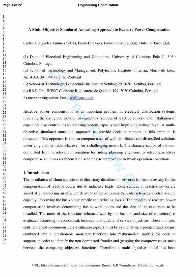
Table 5 presents the objective function values for a representative sample of non-dominated
solutions with different characteristics.
Each point displayed in Figure 6 corresponds to a physical compensation scheme (decision
variable space). A set of well-dispersed solutions is given in Table 4 leading to resistive power
losses and cost given in Table 5 (objective function space). For instance, for solution 1, a
capacitor of type 5 is located in node 3, of type 3 in node 4, etc. Solutions 1 and 10 are the
extreme solutions, which optimize individually the active power losses and the cost objective
functions, respectively.
Page 11 of 22
URL: http:/mc.manuscriptcentral.com/geno Email: [email protected]
Engineering Optimization
123456789101112131415161718192021222324252627282930313233343536373839404142434445464748495051525354555657585960

For Peer Review O
nly
Fig. 6 - Non-dominated front obtained with the multi-objective simulated annealing approach
compared with the front computed using NSGA II
Table 4 - Compensation configurations
Solution Compensation scheme (capacitor installed in each node) # capacitors
1 00530070000006000004000000002000000100030001002
02000400007400000100000000000002000050011001000 20
2 00000070000004000000002003000100004000002000004
00004000407000000200000001000400000060000000000 15
3 00000070000007000000000004000000000000002000004
00000006007000000200000000000400000060000000001 11
4 00000000000007000000000005000000000000002000007
00000000700700000000000000000002000070000000000 8
5 00000000000007000000007000000000000000000000000
02000000700700000000000000000000000070000000000 6
6 00000000000007000000007000000000000000000000000
00000000007000000200000000000000000070000000000 5
7 00000000000000007000000005000000000000000000000
00000000000700000000000000000000000070000000000 4
8 00000000000000000000007000000000000000000000000
00000000000700000000000000000000000070000000000 3
9 00000000000000000000000005000000000000000000000
00000000000000000000000000000500000070000000000 3
10 00000000000000000000000000007000000000000000000
00000000000000000000000000000000000000000700000 2
Page 12 of 22
URL: http:/mc.manuscriptcentral.com/geno Email: [email protected]
Engineering Optimization
123456789101112131415161718192021222324252627282930313233343536373839404142434445464748495051525354555657585960
For Peer Review O
nly
Table 5 - Sample of non-dominated solutions (solution id. refers to Figure 6)
Solution Resistive Losses (kW) Cost (€)
1 235.371 80221
2 235.515 67826
3 236.019 57633
4 237.250 48207
5 239.996 39588
6 244.948 32251
7 249.288 27727
8 256.095 22011
9 265.276 18769
10 278.278 14674
These results have been obtained with 10 simulations. The rate of success of each
neighbourhood structure is reported in Table 6.
Table 6 – Percentage of success of each neighbourhood structures
Neighbourhood
Structure
Average feasible
solutions
Average #
solutions directly
included in the
archive
Average #
solutions directly
replacing other
solutions in the
archive
(a) 10.9095 2.395 2.719
(b) 10.8677 5.623 21.372
(c) 11.3256 1.218 18.516
(d) 10.3408 1.337 12.746
(e) 11.3270 0.446 6.336
(f) 11.2471 44.103 1.936
(g) 11.3344 34.619 1.369
(h) 22.6478 10.26 35.005
Note: Structures (a-h) refer to the example in Figure 4 (a-h).
The voltage profiles at each node before and after the optimization with the multi-objective
simulated annealing procedure, as well as results under different network operating conditions
and CPU running times are reported in Appendix C.
Page 13 of 22
URL: http:/mc.manuscriptcentral.com/geno Email: [email protected]
Engineering Optimization
123456789101112131415161718192021222324252627282930313233343536373839404142434445464748495051525354555657585960

For Peer Review O
nly
Even though it cannot perform actual work, reactive power is required to form the magnetic
field in motors and other electric equipment. Therefore, reactive power should be supplied
locally to decrease the loading of lines and transmission system losses as well as to improve the
voltage profile and steady-state and dynamic stability. A decrease in reactive power causes
voltages to fall and a voltage collapse occurs whenever the system is trying to serve much more
load than the voltage can support. Shunt capacitors banks adequately sized and located near the
loads along the distribution feeders provide several benefits in the exploration of distribution
networks, namely in heavy load periods. Shunt capacitors are generally simple devices, in
which an insulating dielectric is placed between two metal plates. Capacitors installed in
distribution networks may be pole-mounted (least expensive, providing up to 3000 kVAr) or
pad-mounted (generally placed underground). These devices may be controlled either locally or
centrally by means of communication systems. Automatic capacitor banks consist of steps
controlled by a reactive power controller, which ensures that the required reactive power is
always connected to the system. The devices may also contribute to improve power quality by
providing harmonic filtering.
5. Conclusions
Reactive power compensation is a relevant problem in electrical distribution systems. The
adequate sizing and location of capacitors (sources of reactive power that locally supply this
demand) contributes to release system capacity and improve voltage level. The case study
herein presented is a challenging one because the network is lengthy and is operating in adverse
conditions.
A multi-objective simulated annealing approach has been developed, which is specifically
designed to provide decision support for planning tasks in this problem. Findings indicate that
the simulated annealing approach is able to compute a set of well-distributed and diversified
solutions underlying distinct trade-offs between the competing objective functions of
economical and technical nature. The thorough characterization of the non-dominated front is
valuable information for planning engineers in the selection of satisfactory compromise
solutions (compensation schemes) to improve the network operation conditions.
Research is currently underway to design new adequate solution moves and exploit the adaptive
behaviour of neighbourhood structures, also for the sake of replicability in other combinatorial
problems. Moreover, techniques to provide decision support regarding the selection of a
solution for implementation or a set of solutions for further screening are also being developed
taking into account the decision maker's preferences.
Page 14 of 22
URL: http:/mc.manuscriptcentral.com/geno Email: [email protected]
Engineering Optimization
123456789101112131415161718192021222324252627282930313233343536373839404142434445464748495051525354555657585960

For Peer Review O
nly
Acknowledgment
This research has been partially supported by the Portuguese Foundation for Science and
Technology under Project Grant PTDC/ENR/64971/2006 “Multi-objective Models in Energy
Efficiency Evaluation Problems”.
References
C. H. Antunes. C. Barrico. A. Gomes. D. F. Pires and A. G. Martins. “An evolutionary
algorithm for reactive power compensation in radial distribution networks”, Applied Energy, 86
(7-8), 977-984, 2009.
F. Glover and G. A. Kochenberger (Eds.). Handbook of Metaheuristics, Kluwer Academic
Publishers, London, 2003.
H. Kubotani and K. Yoshimura. “Performance evaluation of acceptance probability functions
multi-objective SA”, Computers & Operations Research, 30 (3), 427-442, 2003.
D. F. Pires, C. H. Antunes and A. G. Martins. “An NSGA-II approach with Local Search for a
VAR Planning Multi-Objective Problem”, INESC Coimbra Research Report no. 8, 2009.
http://www.inescc.pt/documentos/RR8_2009_PiresAntunesMartins.pdf.
B. Suman and P. Kumar. “A survey of simulated annealing as a tool for single and
multiobjective optimization”. Journal of the Operational Research Society, 57 (10), 1143-1160,
2006.
W. Zhang, F. Li and L. Tolbert. “Review of reactive power planning: objectives, constraints,
and algorithms”, IEEE Trans. on Power Systems, 22 (4), 2177-2186, 2007.
Page 15 of 22
URL: http:/mc.manuscriptcentral.com/geno Email: [email protected]
Engineering Optimization
123456789101112131415161718192021222324252627282930313233343536373839404142434445464748495051525354555657585960

For Peer Review O
nly
Appendix A – Multi-objective mathematical model
Figure A.1 illustrates the meaning of the variables and parameters associated with in the
electrical network. A feeder is characterized by a resistance, r, and a reactance, x, value
(measured in Ohms, Ω), which constitute the characteristic impedance of the power line, Z .
Fig. A.1 - Electrical feeder and corresponding variables
SB – Substation;
k – iteration number;
t – next bus index;
m – previous bus index;
M – number of network buses;
Bm – bus m;
Y – maximum number of capacitors that can be installed;
mP - active power vector entering bus m;
mQ - reactive power vector entering bus m;
mS - apparent power vector entering bus m;
CmQ - reactive compensation installed in bus m;
CmS - apparent compensation power vector installed in bus m;
LmP - active power demand vector at bus m;
LmQ - reactive power demand vector at bus m;
LmS - apparent power demand vector at bus m;
Plosses(m )- total active power losses vector in all branches subsequent to bus m;
Qlosses(m )- total reactive power losses vector in all branches subsequent to bus m;
S losses(m )- total apparent power losses vector in all branches subsequent to bus m;
mV - root mean square (rms) voltage vector of bus m;
δm –voltage angle in bus m;
mI - current vector that enter bus m;
mtr - resistance of the connection branch from bus m to bus t branch;
mtx - reactance of the connection branch from bus m to bus t branch;
mtZ - impedance of the connection branch from bus m to bus t branch;
QFu –capacity of capacitor of type u;
Cu – cost of capacitor of type u; *X - conjugate vector of a generic vector X .
Page 16 of 22
URL: http:/mc.manuscriptcentral.com/geno Email: [email protected]
Engineering Optimization
123456789101112131415161718192021222324252627282930313233343536373839404142434445464748495051525354555657585960

For Peer Review O
nly
dm – real part of voltage vector.
em – imaginary part of voltage vector.
am
u - binary decision variable denoting whether or not a capacitor of type u is installed in Bm
bm – coefficient denoting whether or not it is technically possible to install a capacitor in Bm
The vectors structure is described in equations (A.1) to (A.6):
mtmtmt jxrZ += (A.1)
mmm jQPS += (A.2)
mmm jedV += (A.3)
LmLmLm jQPS += (A.4)
CmCm jQS −= (A.5)
)()()( mlossesmlossesmlosses jQPS += (A.6)
The apparent power equation at bus m is written as
CmLm
n
i it
ititm
n
i
itm SSV
SV S= S ++
×+ ∑∑
=
∗
+
++
=+
0
)(
0
(A.7)
Active and reactive powers can be obtained by calculating the real and imaginary parts of
mS respectively, (A.8) and (A.9)
)Re( mm SP = (A.8)
)Im( mm SQ = (A.9)
Apparent power is computed from the last bus of the branch to the first bus, and voltages are
computed from the first bus to the last one of the network. The new power values calculated are
immediately used in their predecessors’ equations and the new voltage values calculated are
immediately used in their successors’ equations.
The objective functions are the minimization of the system resistive losses (A.10) and the
capacitor installation cost (A.11):
Page 17 of 22
URL: http:/mc.manuscriptcentral.com/geno Email: [email protected]
Engineering Optimization
123456789101112131415161718192021222324252627282930313233343536373839404142434445464748495051525354555657585960

For Peer Review O
nly
Min ∑ ∑
×
=
∗
+
++
M
1=m 0
)(Ren
i it
ititm
V
SV (A.10)
The index t denotes the identification of the first bus of the lateral.
Min am
u c j
u = 1
Y
∑m =0
M
∑ (A.11)
am
u =1 if the new capacitor QFu is installed in Bm
0 otherwise
(A.12)
=otherwise 0
at capacitor a locate topossible isit if 1m
B
mb
(A.13)
The coefficients bm represent the technical feasibility of installing capacitors at Bm.
QC m=bm am
u QFu
u = 1
Y
∑ ∀ m (A.14)
am
u =1u = 1
Y
∑ ,∀m (A.15)
The upper and lower bounds for the nodes voltage magnitude is given in (A.16).
m V V V m ∀≤≤ maxmin (A.16)
This model is nonlinear and contains both discrete and continuous variables.
Page 18 of 22
URL: http:/mc.manuscriptcentral.com/geno Email: [email protected]
Engineering Optimization
123456789101112131415161718192021222324252627282930313233343536373839404142434445464748495051525354555657585960

For Peer Review O
nly
Appendix B - Selection of the acceptance probability function
This appendix reports some results of the computational experiments carried out in the phase of
tuning the acceptance probability function for the multi-objective problem. Considering the
same initial solutions and the same input parameters, the results of each acceptance probability
function (10 simulations) are presented in Figure B.1 and Table B.1. The results obtained for
each acceptance probability function are similar. The weak rule tends to generate solutions
closer to the individual optima of each objective function, and the scalar linear rule gives
mostly origin to solutions closer to the best values of the resistive losses objective function. In
general, the logistic curve rule and the Chebycheff rule produce solutions well spread in the
non-dominated front.
Fig. B.1 - Comparison between the non-dominated fronts of all simulations for each
acceptance probability function
Page 19 of 22
URL: http:/mc.manuscriptcentral.com/geno Email: [email protected]
Engineering Optimization
123456789101112131415161718192021222324252627282930313233343536373839404142434445464748495051525354555657585960

For Peer Review O
nly
Table B.1 – Comparison between the non-dominated fronts (NDF) for each acceptance
probability function
Probability
functions # NDF
Minimum
Losses
Minimum
Cost
Largest
consecutive
#acceptances
Acceptation
vs.
Rejection
Time (s)
Logistic Curve
Rule 64.5 236.662 17114.1 49.9
50.66% vs.
49.34% 13.081
Scalar Linear
Rule 63.9 236.527 17229.5 50.2
51.25% vs.
48.75 13.991
Chebyshev Rule 58.8 236.734 17641.8 3.6
4.87% vs.
95.13% 7.0744
Weak Rule 78.2 236.163 15208.6 167.5
92.44% vs.
7.56% 77.6
Note: These values are 10 simulations averages for each probability function.
Page 20 of 22
URL: http:/mc.manuscriptcentral.com/geno Email: [email protected]
Engineering Optimization
123456789101112131415161718192021222324252627282930313233343536373839404142434445464748495051525354555657585960
For Peer Review O
nly
Appendix C - Voltage profiles, network operating conditions and CPU times.
Voltage profiles
The study has been carried out for peak load conditions. The active power losses are 320.44
kW. The number of nodes not satisfying the voltage lower bounds is 39 (in 94 nodes; nodes 16-
33 and 74-94), with a minimum 0.8697 (in p.u., that is, with respect to the sub-station SE in
which V= 15.75 kV) in node 33 (see Fig. 5). The voltage profiles after optimization respect the
lower bounds, with a minimum ranging between 0.9004 in node 94 for solution 10 (the
individual optimum to the cost objective function) and 0.9268 in node 33 for solution 1 (the
individual optimum to the resistive losses objective function).
Results for different network operating conditions
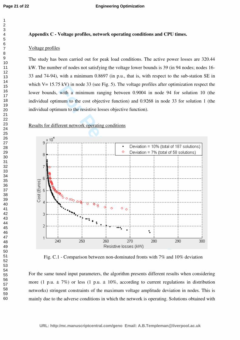
Fig. C.1 - Comparison between non-dominated fronts with 7% and 10% deviation
For the same tuned input parameters, the algorithm presents different results when considering
more (1 p.u. ± 7%) or less (1 p.u. ± 10%, according to current regulations in distribution
networks) stringent constraints of the maximum voltage amplitude deviation in nodes. This is
mainly due to the adverse conditions in which the network is operating. Solutions obtained with
Page 21 of 22
URL: http:/mc.manuscriptcentral.com/geno Email: [email protected]
Engineering Optimization
123456789101112131415161718192021222324252627282930313233343536373839404142434445464748495051525354555657585960

For Peer Review O
nly
the 1 p.u. ± 10% constraint become infeasible for 1 p.u. ± 7% and the non-dominated front is
not as diverse as in the former case because the scope of solutions become narrower.
CPU time and other computational statistical data
Table C.1 – CPU time for different network operating conditions (7% and 10% deviation),
including the time spent in running - and number of calls to - the power flow algorithm (10
runs).
CPU time 1 2 3 4 5 6 7 8 9 10
Deviation=7%
Total time (s): 385.201 282.744 300.385 337.387 309.612 361.033 367.741 368.348 360.874 368.949
Power Flow time (s): 291.270 217.236 227.182 256.923 233.207 274.203 280.638 277.809 270.200 276.548
Power Flow calls (num): 150616 111558 118800 133271 122926 141310 144920 144434 141851 144121
Power Flow time (%): 75.62 76.83 75.63 76.15 75.32 75.95 76.31 75.42 74.87 74.96
MOSA time (s): 93.931 65.508 73.203 80.464 76.405 86.830 87.103 90.539 90.674 92.401
MOSA time (%): 24.38 23.17 24.37 23.85 24.68 24.05 23.69 24.58 25.13 25.04
Deviation=10%
Total time (s): 958.00 1005.00 786.00 825.00 976.00 971.00 1028.00 856.00 1040.00 854.00
Power Flow time (s): 313.491 330.702 257.296 270.934 323.386 323.505 339.128 284.459 346.474 280.557
Power Flow calls (num): 590600 616420 501528 520671 598234 598110 625265 537651 631962 536478
Power Flow time (%): 32.72 32.91 32.73 32.84 33.13 33.32 32.99 33.23 33.31 32.85
MOSA time (s): 644.509 674.298 528.704 554.066 652.614 647.495 688.872 571.541 693.526 573.443
MOSA time (%): 67.28 67.09 67.27 67.16 66.87 66.68 67.01 66.77 66.69 67.15
Table C.2 – Minimum, maximum and average CPU time for different network operating
conditions (7% and 10% deviation), including the time spent in running - and number of calls to
- the power flow algorithm (10 runs).
Deviation=7% Min. Max. Average
Total time (s): 282.744 385.201 344.227
Power Flow time (s): 217.236 291.27 260.522
Power Flow calls (num): 111558 150616 135380.7
Power Flow time (%): 74.87 76.83 75.71
MOSA time (s): 65.508 93.931 83.706
MOSA time (%): 23.17 25.13 24.29
Deviation=10% Min. Max. Average
Total time (s): 786 1040 929.9
Power Flow time (s): 257.296 346.474 306.993
Power Flow calls (num): 501528 631962 575691.9
Power Flow time (%): 32.72 33.32 33.00
MOSA time (s): 528.704 693.526 622.907
MOSA time (%): 66.68 67.28 67.00
Page 22 of 22
URL: http:/mc.manuscriptcentral.com/geno Email: [email protected]
Engineering Optimization
123456789101112131415161718192021222324252627282930313233343536373839404142434445464748495051525354555657585960