ORNL/TM-2005/549

A Multi-Stage Model for Scuffing of Reciprocating Components with Special Consideration of Fuel Injector Plungers

September 2005

Prepared by Peter J. Blau, Principal Investigator with Jun Qu and John J. Truhan, Jr.

DOCUMENT AVAILABILITY Reports produced after January 1, 1996, are generally available free via the U.S. Department of Energy (DOE) Information Bridge:

Web site: http://www.osti.gov/bridge Reports produced before January 1, 1996, may be purchased by members of the public from the following source:

National Technical Information Service 5285 Port Royal Road Springfield, VA 22161 Telephone: 703-605-6000 (1-800-553-6847) TDD: 703-487-4639 Fax: 703-605-6900 E-mail: info@ntis.fedworld.gov Web site: http://www.ntis.gov/support/ordernowabout.htm

Reports are available to DOE employees, DOE contractors, Energy Technology Data Exchange (ETDE) representatives, and International Nuclear Information System (INIS) representatives from the following source:

Office of Scientific and Technical Information P.O. Box 62 Oak Ridge, TN 37831 Telephone: 865-576-8401 Fax: 865-576-5728 E-mail: reports@adonis.osti.gov Web site: http://www.osti.gov/contact.html

This report was prepared as an account of work sponsored by an agency of the United States Government. Neither the United States government nor any agency thereof, nor any of their employees, makes any warranty, express or implied, or assumes any legal liability or responsibility for the accuracy, completeness, or usefulness of any information, apparatus, product, or process disclosed, or represents that its use would not infringe privately owned rights. Reference herein to any specific commercial product, process, or service by trade name, trademark, manufacturer, or otherwise, does not necessarily constitute or imply its endorsement, recommendation, or favoring by the United States Government or any agency thereof. The views and opinions of authors expressed herein do not necessarily state or reflect those of the United States Government or any agency thereof.

ORNL/TM-2005/549

A Multi-Stage Model for Scuffing of Reciprocating Components with Special Consideration of Fuel Injector Plungers

Peter J. Blau1, Principal Investigator with

Jun Qu1, and John J. Truhan, Jr.2

1) Metals and Ceramics Division, Oak Ridge National Laboratory 2) University of Tennessee, Knoxville

Project Milestone Report September 2005

Prepared by OAK RIDGE NATIONAL LABORATORY P.O. Box 2008 Oak Ridge, Tennessee 37831-6285 managed by UT-Battelle, LLC for the U.S. DEPARTMENT OF ENERGY under contract DE-AC05-00OR22725

CONTENTS

List of Figures .................................................................................................................................... v

Foreword............................................................................................................................................ vii

1. Background........................................................................................................................... 1

2. Scuffing at Macro- and Micro-scales……………………………….................................... 2

3. Representation of Regime I…………………………………………................................... 3

4. Boundary Film Failure and the Initiation of Scuffing …………………….......................... 4

5. Surface Roughness Changes…………………………………………….. ........................... 6

6. Length of the Transition Period…………………………………………. ........................... 7

7. The Friction Coefficient as an Indicator of Scuffing…………………. ............................... 8

8. Role of the Shear Strength of Boundary films……………………………… ...................... 9

9. Solid Contact with Significant Deformation (Regime III)………………............................ 11

10. Conclusions…………………………………………………….. ......................................... 16

References……………………………………………………………….. ........................................ 16

iii

LIST OF FIGURES Figure Page 1. Conceptual scuffing model ................................................................................................... 2 2. Schematic representation of a cylindrical plunger with an area of wear damage. The inset suggests that the contact area is comprised of smaller load-bearing patches. ..... 2 3. Portrayal of a finite-length Regime I with various transition rates ....................................... 4 4. Film thickness ratios for various values of composite roughness and film thickness........... 5 5. Quasi-sigmoidal representation of the start and finish of a transition in composite surface roughness at the ends and central portion of an oscillating contact ...................................... 7 6. Data from reciprocating pin-on-twin pins tests suggest that the maximum transition period corresponds to an intermediate value of composite roughness. Data from [9]. .................. 8 7. Friction coefficient as a function of the position and time of contact................................... 9 8. Relationship between the ST parameter and the initiation period for scuffing in reciprocating sliding in Jet A, low sulfur fuel....................................................................... 15

v

FOREWORD The majority of heavy trucks that populate the nation’s highways are powered by diesel engines. According to the latest available statistics,* there were 2.3 M registered combination trucks (those that pull trailers) and they consumed 26.5 B gallons of gas in 2002,averaging 5.2 miles per gallon of fuel. In addition, heavy single-unit trucks consumed 10.3 B gallons of fuel that same year and averaged a slightly-higher 7.4 miles per gallon. Motivated by fuel economy benefits and tighter emission regulations, the Department of Energy has invested in research to improve diesel engine technology, and some of those design improvements place increasing demands on the fuel system components. Friction, wear, and surface damage must be minimized to enable the fuel injectors to provide precisely metered quantities of fuel while smoothly sliding back and forth millions of times over their lifetime. Scuffing is a form of surface damage that can cause fuel injector parts to malfunction. Therefore it is important to understand the mechanisms of scuffing and how to utilize advanced materials and surface treatments to reduce or eliminate its deleterious effects. The model described in this report summarizes a multi-year effort that involved: development of new test methods to evaluate scuffing in reciprocating components, development of quantitative criteria to portray the initiation and propagation of scuffing damage, formulating a graphic method to enable scuffing to be displayed, and developing a model to explain scuffing behavior fundamentally and to serve as a guide for selecting more scuff-resistant materials. During the course of these studies, several open-literature publications were prepared, and these contain a more comprehensive description of the background research than does the present report which focuses mainly on the modeling aspects of the work. It is hoped that the approaches and insights provided here will enable further progress in engine materials technology aimed at fuel savings and emission reduction. Research sponsored by the Heavy Vehicle Propulsion Materials Program, DOE Office of FreedomCAR and Vehicle Technologies Program, under contract DE-AC05-00OR22725 with UT-Battelle, LLC. P. J. Blau Metals and Ceramics Division Oak Ridge National Laboratory * “Transportation Energy Data Book,” 24th Edition, May 2005, available on-line at <http://cta.ornl.gov/data/index.shtml>

vii

1.0 BACKGROUND Scuffing is a form of mechanical surface damage that is often associated with the failure of lubrication to prevent solid/solid contact between moving parts. It manifests itself in a variety of forms, and therefore the term scuffing is not applied consistently throughout the engineering literature. Sometimes it is seen as a form of abrasion. Other times it is seen as a smearing of material that either polishes the surface or roughens it. This diverse usage has made it impossible to define the term precisely and in a universally-applicable way. In this work, scuffing is viewed as a form of sliding contact damage that alters the roughness of mating parts so as to impede their smooth operation. It does not necessary produce loose wear particles, as in wear. Scuffing of diesel engine components, such as those in the fuel system, is the focus of this work. In such applications, the direction of sliding motion reverses rapidly and repeatedly. Parts experience hundreds of thousands, if not millions, of cycles in their lifetimes. Scuffing may be suppressed for a long time, then appear suddenly and cause problems such as part seizure. A milestone report, dated March 2004, described the reciprocating sliding experiments whose results led to the conceptual framework for a three-regime model for scuffing [1]. That model considers the failure of a lubricating film and the increased deformation of the contact surfaces that eventually produce the surface damage referred to as scuffing. It represents an interdisciplinary approach to integrating concepts from both lubrication theory and material science. The model, shown in Figure 1, uses sub-models whose applicability depends on whether the contact is effectively lubricated (solid surfaces that are not touching), boundary-lubricated, or subjected to significant solid contact. The higher the contact pressure, the less likely the lubricant will effectively separate the moving surfaces. Embodied within the current conceptual model is a scuffing process that involves a sequence of three regimes or stages. First, there is a period of effective operation whose duration depends on the nature of the materials, mechanical design and operating parameters, surface finish, and the regime of lubrication. Parts can perform very effectively in Regime I for millions of cycles if all goes well. However, the system can also operate in a boundary lubrication regime (II) in which some solid contact occurs. As plastic deformation begins, there is a change in surface roughness. Surface roughness usually starts smooth and roughens, but that is not always true. Some rough surfaces can become smoother during running-in, then roughen again much later due to wear-out. The distribution, thickness, and shear characteristics of the lubricating film can change as the lubricants age in situ. The directionality of machined surface features can change due to mechanical texturing during wear. In many practical systems, scuffing begins at one part of the contact surface and then spreads out until the whole surface is altered. A significant exception to that effect is when severe galling causes surfaces to seize, halting relative motion entirely.

1

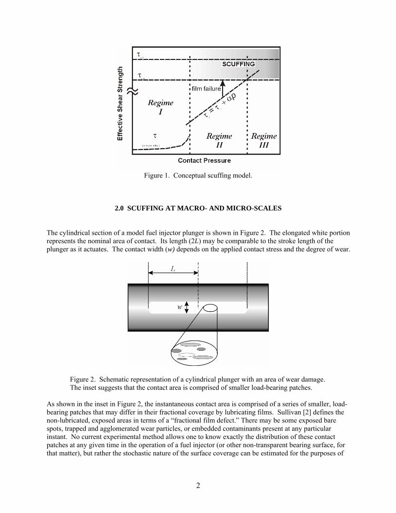
Figure 1. Conceptual scuffing model.

2.0 SCUFFING AT MACRO- AND MICRO-SCALES The cylindrical section of a model fuel injector plunger is shown in Figure 2. The elongated white portion represents the nominal area of contact. Its length (2L) may be comparable to the stroke length of the plunger as it actuates. The contact width (w) depends on the applied contact stress and the degree of wear.

Figure 2. Schematic representation of a cylindrical plunger with an area of wear damage. The inset suggests that the contact area is comprised of smaller load-bearing patches.

As shown in the inset in Figure 2, the instantaneous contact area is comprised of a series of smaller, load-bearing patches that may differ in their fractional coverage by lubricating films. Sullivan [2] defines the non-lubricated, exposed areas in terms of a “fractional film defect.” There may be some exposed bare spots, trapped and agglomerated wear particles, or embedded contaminants present at any particular instant. No current experimental method allows one to know exactly the distribution of these contact patches at any given time in the operation of a fuel injector (or other non-transparent bearing surface, for that matter), but rather the stochastic nature of the surface coverage can be estimated for the purposes of

2

modeling. Examination of scuffed surfaces after the fact shows only the contact arrangement that occurred after the last operating stroke. In developing the model, particular focus was placed on Regime II where the lubricant begins to fail, allowing more and more intermittent surface contact and changing surface roughness due to material deformation on a local scale. By the time Regime III has occurred, the parts have scuffed significantly and the end of part life is near.

3.0 REPRESENTATION OF REGIME I Regime I is characterized by a full-film of lubricant separating the surfaces. The occurrence and duration of Regime I will depend on the design (macrocontact) of the components, the stability of the relative motion, the surface finish, and the lubricant condition. Ideally, the lifetime of the component will remain entirely within Regime I, and some other failure mode, other than scuffing, will mark its end-of-life. However, as the components and the lubricants age, or if the contact pressure is too large to sustain a full film condition, then Regime I may either be finite in length or not observed at all. Considering the case in which there is an initial film with a finite effective performance life, one can express the shear strength in the interface in terms of the friction coefficient. If the duration of contact is expressed in terms of numbers of oscillating cycles, as in a fuel injector plunger, then the transition from Regime I to Regime II can be expressed as follows:

n

ffx Lx

⎟⎠⎞

⎜⎝⎛∆+= µµµ (1)

where µx = friction coefficient at x cycles µff = friction coefficient for full-film lubrication ∆µ = change in friction during the transition from full-film to boundary lubrication x = current number of oscillating cycles L = number of cycles to reach Regime II n = a constant to reflect the rate of change during the transition period. In Eq. (1), in practical cases one can further express the change in friction as follows: ∆µ = µbl - µff (2) where µbl the friction coefficient for boundary lubrication at the start of Regime II. Assigning typical values of µff = 0.01, µbl = 0.12, and letting L = 1,000,000 cycles, we can plot Eq. (1) for a finite life in Regime I for several rates of transition (see Figure 3). The large magnitude of the rate constant (n) reflects the condition in which the vast majority of the life in Regime I is relatively stable, and only at the end of this stable period does the transition become noticeable and significant. Physically, the exponent n would reflect such processes as a loss in lubricant load carrying capacity from degradation (in closed systems), a change in the contamination level in the system due to debris build-up

3

or contaminant entrainment, or even swelling of the plunger material to reduce bore clearance and increase surface contact. Having established an expression for Regime I, the challenge arises of understanding and representing the intricacies of Regime II in which the precursors for scuffing take shape under boundary lubrication.

0.00

0.05

0.10

0.15

0.20

0 2 105 4 105 6 105 8 105 1 106 1.2 106

Regime I

n = 10n = 5

µx

CYCLES

µff = 0.01

µbl

= 0.12

Figure 3. Portrayal of a finite-length Regime I with various transition rates.

4.0 BOUNDARY FILM FAILURE AND THE INITIATION OF SCUFFING The film thickness ratio (Λ) is a convenient parameter to relate the composite surface roughness (σ) of the two contacting surfaces (Eq. 1 and 2) to the nominal thickness (h) of the lubricating film that separates them. It is defined in Equation (3):

22

21 σσ +

=Λh (3)

The thicker the lubricating film, the higher the Λ, at a given composite roughness. In approximate terms, when Λ ≤ 1, the lubricant cannot fully separate the surfaces, but when Λ ≥ 3, a full lubricating film may be developed between surfaces. Between these values, the lubrication regime can be considered a mixture of these two situations. Generally, the friction coefficient drops as Λ increases. Depending upon the relative hardness of the mating surfaces, the method of their preparation, and the applied load on the bodies, the surface roughness may not be the same on the two opposing surfaces. Further, due to running-in effects when under less than complete surface separation, the roughness of one or both surfaces tends to change during use.

4

The film thickness can also change with time, especially if the temperature or pressure in the system changes. This effect is commonly represented for Newtonian fluids by an equation developed by Dowson and Hamrock [3], and it was discussed earlier by Dowson in terms of a micro-rheodynamic film in which films are entrained between asperities [4]: (4) ( ) 3/13/207.1 rUh s ⋅= αη where α = pressure-viscosity coefficient η = fluid viscosity Us = sliding speed r = the composite radius of two interacting asperities of radii r1 and r2, defined as follows:

21

21

rrrrr

+= (5)

Therefore, all three variables that define the instantaneous Λ value for a sliding contact have the potential to be time-dependent, and the regime of lubrication may fluctuate both locally and throughout the contact. The relationships between various quantities can be demonstrated by holding certain variables constant and allowing others to change. For example, Figure 4 shows the boundaries between various lubrication regimes as a function of the composite roughness of the two surfaces with several film thicknesses.

0.1

1.0

10.0

0.0 0.2 0.4 0.6 0.8 1.0 1.2

FULL FILM

h = 0.05h = 0.1h = 0.2h = 0.5h = 1.0

Λ

COMPOSITE ROUGHNESS (µm)

BOUNDARY

MIXED

Figure 4. Film thickness ratios for various values of composite roughness and film thickness.

5

5.0 SURFACE ROUGHNESS CHANGES Increasing the surface roughness increases the contact stress on individual asperities, squeezes out the boundary films [5], thins those films to effectively raise their shear strength (see Ref [6] on properties of confined fluids), transmits force, and deforms the contacting materials first elastically and then plastically. The change in composite roughness (which can directly affect the friction force) at a given location can be represented by a quasi-sigmoidal expression [7]:

( ) ⎪⎭

⎪⎬⎫

⎪⎩

⎪⎨⎧

⎥⎥

⎦

⎤

⎢⎢

⎣

⎡

+−

−++= γγ

σσσ /1

11

2m

mioN

MN

NN (6)

where N = current number of cycles σo = the initial composite roughness σi = incremental change in composite roughness ( = σfinal – σo) σN = composite roughness after N cycles of sliding γ = rate of roughness change Nm = number of cycles to reach the midpoint of the transition Studies of fuel injector materials in reciprocating frictional contact, and under boundary lubricating conditions [8] have indicated that the surface roughening features which signal the onset of scuffing and a rise in friction tend to initiate at the ends of the contact region and gradually spread toward the center of the stroke. Therefore, we expect the transition from low to higher composite roughness to begin earlier at the direction reversal points. If, due to the more effective lubricating characteristics at mid-stroke, the rate constant γ is lower at the center than at the ends of the stroke, as an approximation, one can represent a general expression for the average change in composite roughness:

] ]{ }centerNedgeN σσσ +=21 (7)

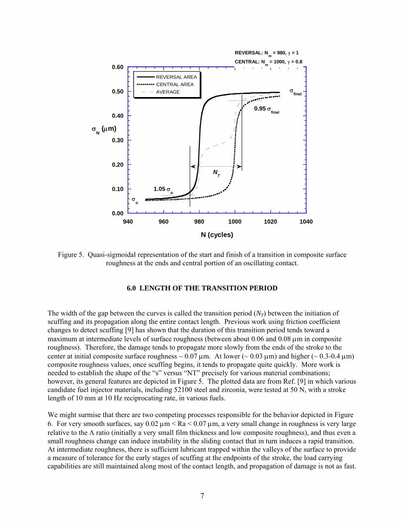
In Eq. (7), the rate constants for the two terms in braces can be independently considered. By means of example, if the composite arithmetic surface roughness begins at Ra = 0.05 µm, a reasonably good polish, and ends at Ra = 0.50 µm, typical of roughening after the onset of scuffing, one can model the transition from smooth to scuffed using Eq. (1). Figure 5 shows form of curves that arise from the use of Eq. (6) and indicate some additional features to be discussed subsequently. The solid line is intended to represent the composite roughness at the reversal point where scuffing generally starts. The transition begins about 20 cycles before the central portion, represented by the dotted line. In this example, the reversal region was given a slightly faster rate factor (γ = 1.0) than the central region (γ = 0.8) to reflect the tendency of the mid-portion of the stroke to scuff more slowly. The intermediate curve (dashes) averages the two curves, and indicates that average roughness versus time can follow a complex shape.

6

0.00

0.10

0.20

0.30

0.40

0.50

0.60

940 960 980 1000 1020 1040

REVERSAL AREACENTRAL AREAAVERAGE

σN (µm)

N (cycles)

REVERSAL: Nm

= 980, γ = 1

CENTRAL: Nm

= 1000, γ = 0.8

NT

0.95 σfinal

1.05 σo

σfinal

σo

Figure 5. Quasi-sigmoidal representation of the start and finish of a transition in composite surface roughness at the ends and central portion of an oscillating contact.

6.0 LENGTH OF THE TRANSITION PERIOD The width of the gap between the curves is called the transition period (NT) between the initiation of scuffing and its propagation along the entire contact length. Previous work using friction coefficient changes to detect scuffing [9] has shown that the duration of this transition period tends toward a maximum at intermediate levels of surface roughness (between about 0.06 and 0.08 µm in composite roughness). Therefore, the damage tends to propagate more slowly from the ends of the stroke to the center at initial composite surface roughness ~ 0.07 µm. At lower (~ 0.03 µm) and higher (~ 0.3-0.4 µm) composite roughness values, once scuffing begins, it tends to propagate quite quickly. More work is needed to establish the shape of the “s” versus “NT” precisely for various material combinations; however, its general features are depicted in Figure 5. The plotted data are from Ref. [9] in which various candidate fuel injector materials, including 52100 steel and zirconia, were tested at 50 N, with a stroke length of 10 mm at 10 Hz reciprocating rate, in various fuels. We might surmise that there are two competing processes responsible for the behavior depicted in Figure 6. For very smooth surfaces, say 0.02 µm < Ra < 0.07 µm, a very small change in roughness is very large relative to the Λ ratio (initially a very small film thickness and low composite roughness), and thus even a small roughness change can induce instability in the sliding contact that in turn induces a rapid transition. At intermediate roughness, there is sufficient lubricant trapped within the valleys of the surface to provide a measure of tolerance for the early stages of scuffing at the endpoints of the stroke, the load carrying capabilities are still maintained along most of the contact length, and propagation of damage is not as fast.

7

Where the surfaces are rougher, the contact stress on the “sharper” asperities is relatively high, causing boundary films to fail. With higher traction, there is more wear debris (third-body) formation which in turn moves within the interface and accelerates the transition process. Temperatures may rise locally, but when the transition time is short, the externally-observed rise in bulk temperature may significantly lag the transition to the point of gross scuffing and higher friction.

0

500

1000

1500

2000

0 0.1 0.2 0.3 0.4 0.5

Pin-on-twin testsload = 50 N

rate = 10 Hzstroke = 10 mm

fuel lubrication

NT

(cyc

les)

σ Figure 6. Data from reciprocating pin-on-twin pins tests suggest that the maximum transition period (NT)

corresponds to an intermediate value of composite roughness. Data from [9]. NT is very sensitive to σ at low values of σ, but less so at higher values of σ. This suggests that incremental improvements in the surface finishing of injector pins can have a large effect on scuffing when the initial composite roughness is below 0.l µm, and that at the lower σ values, the tribosystem may be highly sensitive (intolerant) to manufacturing imperfections, including small pin alignment errors that cause stress concentrations. Therefore, a less smooth surface with more opportunity for a boundary lubricant to do its work may ultimately be more “forgiving,” even though the sealing capabilities of the plunger-bore fit are reduced. The transition period consists of a complex physical situation in which the relative contributions of boundary films, materials deformation, and contact morphology are changing. These contributions are reflected by the detailed time-dependent characteristics of the friction coefficient.

7.0 THE FRICTION COEFFICIENT AS AN INDICATOR OF SCUFFING Friction coefficient has been used as an indicator for the initiation and propagation of scuffing. Figure 7 is a form of “scuffing map” that shows the friction coefficient versus time for locations along the length of the lower specimen in a self-mated 52100 bearing steel sliding couple. Note that the higher values occur at the ends of the stroke and that slices through the friction coefficient-versus time planes display

8

the kind of quasi-sigmoidal representation that has been used to model the changes in composite surface roughness.

01 2 3

45

78

910

0

120

240360

480600

0.000.010.020.030.040.050.060.070.080.090.100.110.120.130.140.150.160.170.180.190.20

µ

Stroke Location (mm)

Time (s)

0.190-0.2000.180-0.1900.170-0.1800.160-0.1700.150-0.1600.140-0.1500.130-0.1400.120-0.1300.110-0.1200.100-0.110

Figure 7. Friction coefficient as a function of the position and time of contact.

8.0 ROLE OF THE SHEAR STRENGTH OF BOUNDARY FILMS The composite roughness changes in response to increasing surface deformation, but in the boundary lubrication regime, some of the deformation can be avoided if the thin boundary films that coat the surface shear preferentially and protect from full solid/solid contact. The ability of these lubricating films to adequately reduce friction is related to their effective shear stress which, as shown in Fig 3, can be expressed by the linear Zisman equation that takes into account the dependence of shear stress on contact pressure [10]: τ = τo + α p (8) where τ = effective shear stress το = shear stress at zero pressure (an extrapolation of data for a series of non-zero pressures) α = the pressure coefficient of the shear strength p = contact pressure.

9

Typical values of τo and α for metals are given in Table 1 (Ref. [11]). The τo and α values for boundary lubricants are less commonly known, but it is known that liquids can act as plastic solids when trapped between asperities [12].

Table 1. Typical values of τo and α (Ref. [11], collected data).

Metal τo (MPa) α Iron 173.8 0.075 Copper 107.6 0.049 Aluminum 47.6 0.035 Silver 12.3 0.012

As the surface roughness increases, the true area of contact decreases, causing the localized contact pressure to increase. Therefore, if α>0 as it is for the metals in Table 1, the shear strength of the boundary film will also increase, raising the friction until the high spots are sheared off and the surface area decreases again. A boundary film could reform on the smoother patches (see also Fig. 2). This process is reflected in the complex rise and fall of friction during the transition from partial scuffing to a more completely-scuffed state, as exemplified in Fig. 6. A slice of Fig. 6, parallel to the sliding distance axis at either end-of-stroke location, would show the characteristic shape of the friction versus time record for running-in of certain metals. (See ref [11] for a discussion of running-in curve shape “b”.) In this case, the friction coefficient first rises to an initial maximum then falls to a lower, steady-state value. Connection with the composite roughness and the friction coefficient can be appreciated by considering the following simple relationships. The friction force (F) acting over an area (A) is proportional to the shear strength: F = τ A (9) The friction coefficient is defined as the ratio of friction force to normal force P: µ = F / P (10) Combining (8), (9), and (10) gives:

( )P

Apo ατµ

+= (11)

In Regime II, one can assume that the area of contact A after N cycles is locally inversely proportional to the composite roughness after that number of cycles. Note that the quasi-static hardness of a solid is commonly defined as resistance to penetration and can be represented as being proportional to the ratio of load to area:

APcH ≈ (12)

where c = a geometric constant that is related to the indenter shape. There might be a temptation to restate Eq. (11) with the friction coefficient as being inversely proportional to hardness; however, the question arises as to whether that approach is physically correct. In such treatments, the hardness number generally applies to the softer of the two solids in contact. Since

10

scuffing can cause deformation on both contacting surfaces, and because the hardness can change with number of cycles due to workhardening, using the hardness only of the softer surface flies in the face of physical observations of scuffed surfaces. The definition in Eq. (12) also implies quasi-static conditions, but interfacial shear strength can also be affected by shear rate, and therefore it seems doubly inappropriate to interpret the A/P factor in Eq. (11) simply as a kind of “inverse hardness number.” Nevertheless, as composite roughness increases, τ tends to increase because A momentarily decreases. Eventually the peaks will be removed and A may increase again and lower p, but at some point, the higher friction causes removal of the boundary film and the nascent surfaces come into direct contact, raising the friction still higher and causing more severe plastic deformation in the solids. That leads to Regime III.

9.0 SOLID CONTACT WITH SIGNIFICANT DEFORMATION (REGIME III) Regime III can be considered to transcend the realm of light scuffing damage, which can be tolerated in some sliding components, and to enter more serious progressive damage conditions which are known as severe wear or surface damage, such as “galling” or seizure. Earlier in this project a dimensionless measure for scuffing tendency was suggested, namely:

⎟⎠⎞

⎜⎝⎛

⎥⎦

⎤⎢⎣

⎡+⎟⎟

⎠

⎞⎜⎜⎝

⎛==

APf

HHpfff ad

s

hdeftrscuff τ

µ2.1

(13)

where ftr = traction factor fdef = deformation factor fad = adhesion factor µ = friction coefficient P = normal load A = nominal contact area τ = shear strength of the weaker surface of the contact pair p = the penetration factor Hh = scratch hardness of the harder surface Hs = scratch hardness of softer surface. Scratch hardness incorporates dynamic effects not adequately represented by quasi-static hardness numbers such as Vickers, Knoop, Brinell, and Rockwell. In essence, that model embodies the classical treatment of solid friction by Bowden and Tabor [13] as the sum of an adhesive term and one due to plowing. The total solid friction determined in that way is reduced by exposure to a residual lubricant, as is implicit in ftr. While the model may be academically interesting, the values for specific quantities within the expression, especially fad, are not directly measurable. Furthermore, there is no time-dependence explicit in Eqn. (13), assuming that neither Hs nor Hs changes with time. Regime III can be considered to transcend scuffing and enter the more serious modes of surface damage known as severe wear, wear-out, scoring, or galling. Therefore, the form of an expression to describe Regime III needed to be rethought. On the other hand, Regime III surface damage is generally too severe for fuel injectors having tight tolerances, so while academically interesting, its discussion will be kept brief. In Regime III, if seizure does not occur, then the progression of surface damage in the less wear-resistant of the contacting materials can reach a steady-state wear rate that can be approximated by the well-known Archard equation [14]:

11

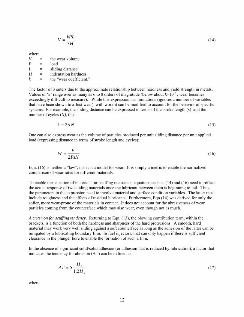
H

kPLV3

= (14)

where V = the wear volume P = load L = sliding distance H = indentation hardness k = the “wear coefficient.” The factor of 3 enters due to the approximate relationship between hardness and yield strength in metals. Values of ‘k’ range over as many as 6 to 8 orders of magnitude (below about k=10-8 , wear becomes exceedingly difficult to measure). While this expression has limitations (ignores a number of variables that have been shown to affect wear), with work it can be modified to account for the behavior of specific systems. For example, the sliding distance can be expressed in terms of the stroke length (s) and the number of cycles (N), thus: L = 2 s N (15) One can also express wear as the volume of particles produced per unit sliding distance per unit applied load (expressing distance in terms of stroke length and cycles):

PsNVW

2= (16)

Eqn. (16) is neither a “law”, nor is it a model for wear. It is simply a metric to enable the normalized comparison of wear rates for different materials. To enable the selection of materials for scuffing resistance, equations such as (14) and (16) need to reflect the actual response of two sliding materials once the lubricant between them is beginning to fail. Thus, the parameters in the expression need to involve material and surface condition variables. The latter must include roughness and the effects of residual lubricants. Furthermore, Eqn (14) was derived for only the softer, more wear-prone of the materials in contact. It does not account for the abrasiveness of wear particles coming from the counterface which may also wear, even though not as much. A criterion for scuffing tendency. Returning to Eqn. (13), the plowing contribution term, within the brackets, is a function of both the hardness and sharpness of the hard protrusions. A smooth, hard material may work very well sliding against a soft counterface as long as the adhesion of the latter can be mitigated by a lubricating boundary film. In fuel injectors, that can only happen if there is sufficient clearance in the plunger bore to enable the formation of such a film. In the absence of significant solid/solid adhesion (or adhesion that is reduced by lubrication), a factor that indicates the tendency for abrasion (AT) can be defined as:

s

h

HH

SAT2.1

= (17)

where

12

Hh = the scratch hardness of the harder side Hs, = the scratch hardness of the softer side S = the deviation from the optimal roughness to delay the onset of scuffing (e.g., see Fig. 5.) The factor 1.2 enters from the classic work by Tabor on hardness that suggests for many materials, there must be about a 20% difference in hardness in order for abrasion to occur [15]. The deviation from the optimum composite surface roughness can be defined:

m

optHHS ,σσ −= (18)

where σH = the hardness-weighted composite roughness

h

ssqhqH H

HRR ⋅+= 2

,2,σ (19)

σH,opt. = the optimal hardness-weighted composite roughness

h

soptsqopthqoptH H

HRR ⋅+= 2

,,2

,,,σ (20)

m = a weighting exponent that reflects the relative importance this function More weight is given to the hardness of the harder side in the definition of composite roughness in Eqs. (19) and (20), because the roughness of the harder side dominates abrasion. When Hh = Hs, σH will be in the regular form (non-weighted) of composite definition. On the other hand, if Hh >> Hs, σH will reflect the hardness of the harder side only. Previously published, reciprocating scuffing test data for a series of materials [8] were used to evaluate scuffing based on the foregoing relationships. Table 2 lists composition and processing information about the materials, and Table 3 shows the mating pairs that were used. Note that the RMS roughness Rq other than average arithmetic roughness Ra is used here for the purpose of composite roughness calculation. Since scratch hardness data was not available for all materials, the Vickers microindentation hardness values were used as an approximation. Previous data for tests [9] showed an optimal composite roughness of 0.07 µm for the steel-steel contact. Zirconia-steel contact exhibited better scuffing resistance at higher composite roughness up to 0.38 µm ( = =0.27 µm) [9], which covers the roughness range for most practical applications, such as the diesel fuel injector systems have the composite roughness around 0.26 µm. Therefore,

= = 0.27 µm is used as the optimal roughness in the present case, and the corresponding σ

opthqR ,, optsqR ,,

opthqR ,, optsqR ,,

H,opt is determined. There was no experimentally-determined optimal roughness for other material combinations, such as the cermet-steel and TiN-steel contacts. Assuming they have similar trends in scuffing resistance-roughness correlation as the zirconia-steel contact, = = 0.27 µm is also used as the optimal roughness for cermet-steel and TiN-steel contacts and the hardness-weighted optimal composite roughness are calculated in Table 3.

opthqR ,, optsqR ,,

13

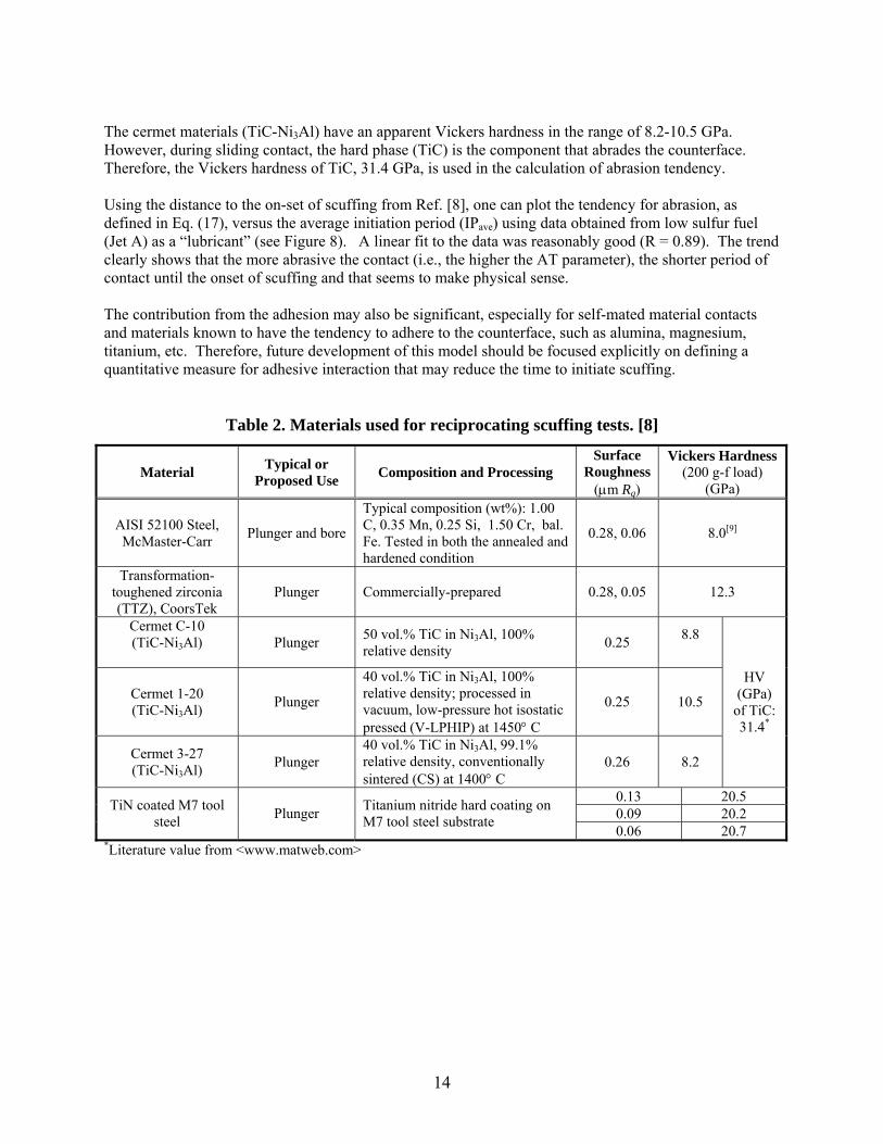
The cermet materials (TiC-Ni3Al) have an apparent Vickers hardness in the range of 8.2-10.5 GPa. However, during sliding contact, the hard phase (TiC) is the component that abrades the counterface. Therefore, the Vickers hardness of TiC, 31.4 GPa, is used in the calculation of abrasion tendency. Using the distance to the on-set of scuffing from Ref. [8], one can plot the tendency for abrasion, as defined in Eq. (17), versus the average initiation period (IPave) using data obtained from low sulfur fuel (Jet A) as a “lubricant” (see Figure 8). A linear fit to the data was reasonably good (R = 0.89). The trend clearly shows that the more abrasive the contact (i.e., the higher the AT parameter), the shorter period of contact until the onset of scuffing and that seems to make physical sense. The contribution from the adhesion may also be significant, especially for self-mated material contacts and materials known to have the tendency to adhere to the counterface, such as alumina, magnesium, titanium, etc. Therefore, future development of this model should be focused explicitly on defining a quantitative measure for adhesive interaction that may reduce the time to initiate scuffing.

Table 2. Materials used for reciprocating scuffing tests. [8]

Material Typical or Proposed Use Composition and Processing

Surface Roughness

(µm Rq)

Vickers Hardness (200 g-f load)

(GPa)

AISI 52100 Steel, McMaster-Carr Plunger and bore

Typical composition (wt%): 1.00 C, 0.35 Mn, 0.25 Si, 1.50 Cr, bal. Fe. Tested in both the annealed and hardened condition

0.28, 0.06 8.0[9]

Transformation-toughened zirconia (TTZ), CoorsTek

Plunger Commercially-prepared 0.28, 0.05 12.3

Cermet C-10 (TiC-Ni3Al)

Plunger 50 vol.% TiC in Ni3Al, 100%

relative density 0.25 8.8

Cermet 1-20 (TiC-Ni3Al) Plunger

40 vol.% TiC in Ni3Al, 100% relative density; processed in vacuum, low-pressure hot isostatic pressed (V-LPHIP) at 1450° C

0.25 10.5

Cermet 3-27 (TiC-Ni3Al) Plunger

40 vol.% TiC in Ni3Al, 99.1% relative density, conventionally sintered (CS) at 1400° C

0.26 8.2

HV (GPa)

of TiC: 31.4*

0.13 20.5 0.09 20.2 TiN coated M7 tool

steel Plunger Titanium nitride hard coating on M7 tool steel substrate 0.06 20.7

*Literature value from <www.matweb.com>

14

Table 3. Scuffing Initiation and Roughness Data for a Series of Sliding Combinations (Counterface material = hardened 52100 steel, Rq = 0.284 µm, HV = 8.0 GPa)

Test material

RMS Rough-ness, Rq

(µm)

Hardness Ratio ( Hh / 1.2 Hs )

(dimensionless)

Optimal Composite Roughness σH,opt (µm)

Composite Roughness

σH (µm)

S (m=1) (µm)

AT [eqn. 17]

(µm)

IPave (m)

52100 steel 0.065 0.833 0.070 0.291 0.221 0.184 6 TiN coated tool st 0.126 2.135 0.318 0.218 0.101 0.215 6 TiN coated tool st 0.088 2.104 0.319 0.199 0.120 0.252 6 TiN coated tool st 0.063 2.156 0.318 0.187 0.130 0.281 6 52100 steel 0.284 0.833 0.070 0.402 0.332 0.276 12 TTZ zirconia 0.05 1.281 0.347 0.234 0.112 0.144 12 Cermet 1-20 0.252 3.271 0.302 0.290 0.013 0.041 18 Cermet C10 0.252 3.271 0.302 0.290 0.013 0.041 24 TTZ zirconia 0.277 1.281 0.347 0.359 0.013 0.016 30 Cermet 3-27 0.265 3.271 0.302 0.301 0.001 0.004 30

0

5

10

15

20

25

30

35

40

0.00 0.05 0.10 0.15 0.20 0.25 0.30

IPav

e (m)

AT (µm)

IP(ave) = M0 + M1*AT26.53M0

-79.30M10.892R

Figure 8. Relationship between the AT parameter and the initiation period for scuffing (IPave) in reciprocating sliding in Jet A, low sulfur fuel.

The contribution from the adhesion between self-mated steels may be significant, and this factor may have caused the data for 52100 steel to be less-well correlated than that of the other materials. Therefore, future development of this model should be focused explicitly on defining a quantitative measure for adhesive interaction that would be expected to reduce the time to initiate scuffing.

15

10. CONCLUSIONS Modeling of the scuffing process must be tailored to the specific tribosystem in which the phenomenon occurs and a general scuffing model is not feasible. In reciprocating systems, such as the fuel injector plunger, lubricating films are difficult to establish and in most common cases, a state of boundary or starved lubrication exists. Based on observations, a three-stage model was developed that incorporates the lubrication regime, protection of the solids by boundary films, initial and evolving surface roughness, and the relative hardness of the sliding materials. The first stage involves lubrication by fluid films and in principle could last indefinitely if not disturbed. The duration of the second stage is dependent on the load-bearing characteristics of thin boundary films or reaction products created from lubricant additive chemistry. The third involves the mechanical properties of the solids, specifically the shear strength and resistance to penetration. A parametric model that describes scuffing resistance to plowing was observed to correlate reasonably well with a series of ceramics, cermets, and hard coatings sliding against 52100 steel, a common fuel injector bore material. However, additional research is needed to quantify the influence of adhesion tendency, a factor that more significantly affects self-mated materials under starved lubrication, and that may reduce the scuffing initiation period below what is predicted by the plowing-related scuffing parameter presented here.

REFERENCES 1. P.J. Blau, J. Qu, and J.J. Truhan, Jr.(2004). “On the Definition and Mechanisms of Scuffing in Fuel

System Components: an Integrated Process Model,” Project milestone report, Sept. 30, 2004. 2. J. L. Sullivan (1986). “Boundary lubrication and oxidational wear,” J. Phys. D.: Appl. Phys., 19, pp.

1999-2011. 3. B.J. Hamrock, D. Dowson. Ball Bearing Lubrication – The Elastohydrodynamics of Elliptical

Contacts, John Wiley & Sons, 1981, p. 212. 4. D. Dowson (1970). “Elastohydrodynamic lubrication,” in Interdisciplinary Approach to Friction and

Wear, NASA Special Pub. SP-237, p. 27. 5. S. Zilberman, B. N. J. Persson, A. Nitzan, F. Mugele, and M. Salmeron (2001). “Boundary

lubrication: Dynamics of squeeze-out,” Phys. Rev. E., 63, 055103-(1-4). 6. G. Luengo, J. Israelachvili, and S. Granick (1996). “Generalized effects in confined fluids: new

friction map for boundary lubrication,” Wear, 200, pp. 328-335. 7. P. J. Blau (1987). “A Model for Run-In and Other Transitions in Sliding Friction”, J. of Tribology,

109, pp. 537-544. 8. J. Qu, J. J. Truhan, and P. J. Blau (2005). “Investigation of the scuffing characteristics of candidate

materials for heavy duty diesel fuel injectors,” Tribology Intl., 38(4), pp. 381-390.

16

9. J. Qu, J. J. Truhan, P. J. Blau, and H. M. Meyer (2005). “Scuffing transition diagrams for heavy duty diesel fuel injector materials in ultra low-sulfur fuel-lubricated environments,” Wear, 259, pp. 1031-1040.

10. W. Zisman (1959). Proc. Symposium on Friction and Wear, ed. R. Davis, Elsevier, pp. 110-148. 11. P. J. Blau (1996). Friction Science and Technology, Marcel Dekker, New York. 12. R. S. Fein (1987). “Characteristics of Boundary Lubrication,” in Handbook of Lubrication, Vol. II,

ed. E. R. Booser, CRC Press, Boca Raton, FL. 13. F. P. Bowden and D. Tabor (1986). Friction and Lubrication of Solids, Oxford Press, 1986. 14. J. F. Archard (1980). “Wear Theory and Mechanisms,” in Wear Control Handbook, ed. W. O. Winer

and M. B. Peterson, ASME, New York, pp. 35-80. 15. D. Tabor (1951). The Hardness of Metals, Oxford Press, UK.

17

18

ORNL/TM-2005/549

INTERNAL DISTRIBUTION 1. – 5. P. Blau, Bldg 4515, MS 6063 9. P. S. Sklad, Bldg 4515, MS 6065

6. D. R. Johnson, Bldg 4515, MS 6066 10. T. N. Tiegs, Bldg 4508, MS 6087

7. E. Lara-Curzio, Bldg 4515, MS 6069 11. J. J. Truhan, Jr., Bldg 4515, MS 6063

8. J. Qu, Bldg 4515, MS 6063 12. A. A. Wereszczak, Bldg 4515, MS 6068

13. ORNL Office of Technical Information & Classification – RC

EXTERNAL DISTRIBUTION 14. Valery Dunaevsky, Bendix Commercial Vehicle Systems, 901 Cleveland St., Elyria, OH 44126 15. - 19. James J. Eberhardt, Office of FreedomCAR and Vehicle Technology, U.S. Dept. of Energy,

1000 Independence Avenue SW, Washington, DC 20585 (5 copies) 20. George Fenske, Argonne National Laboratory, Bldg 212, 9700 S. Cass Avenue, Argonne, IL 60439 21. George Hansen, Detroit Diesel Corporation, 13400 Outer Drive W, Detroit, MI 48329-4001 22. S. M. Hsu, National Institute of Standards and Technology, Room A-265, Building 223,

Gaithersburg, MD 20899 23. Yuri Kalish, Detroit Diesel Corporation, 13400 Outer Drive W, Detroit, MI 48329-4001 24. Prof. Kenneth C. Ludema, 3430 Windemere Ct, Ann Arbor, MI 48105 25. O. Ojayi, Argonne National Laboratory, Bldg 212, 9700 S Cass Avenue, Argonne, IL 60439 26. Larry Seitzman, Caterpillar Inc., Tech. Center, P. O. Box 1875, Peoria, IL 61656-1875 27. Dr. Steven J. Shaffer, Battelle Memorial Institute, 505 King Ave, Columbus, OH 43201-2693 28. Jeremy Trethewey, Advanced Materials Technology, Caterpillar Inc., Tech. Center, P. O. Box 1875,

Peoria, IL 61656-1875 29. Simon Tung, General Motors R&D, Fuel and Lubricants, P. O. Box 9055 (30500 Mound Road),

Warren, MI 48090-9055 30. D. E. Wittmer, Department of Mechanical Engineering and Energy Processes, Southern Illinois

University, Carbondale, IL 62901-6603 31. Thomas Yonushonis, Cummins Engine Company, Inc., 1900 McKinley Ave, MC: 50183,

Columbus, IN 47201