A multiscale multilayer vertically integrated model …boguo/pdfs/publications/2016_Guo_et_al...A multiscale multilayer vertically integrated model with ... 2 sequestration in layered

RESEARCH ARTICLE10.1002/2016WR018714

A multiscale multilayer vertically integrated model with verticaldynamics for CO2 sequestration in layered geologicalformationsBo Guo1, Karl W. Bandilla1, Jan M. Nordbotten1,2, Michael A. Celia1, Eirik Keilegavlen2, andFlorian Doster3

1Department of Civil and Environmental Engineering, Princeton University, Princeton, New Jersey, USA, 2Department ofMathematics, University of Bergen, Bergen, Norway, 3Institute of Petroleum Engineering, Heriot-Watt University,Edinburgh, UK

Abstract Efficient computational models are desirable for simulation of large-scale geological CO2

sequestration. Vertically integrated models, which take advantage of dimension reduction, offer one type ofcomputationally efficient model. The dimension reduction is usually achieved by vertical integration basedon the vertical equilibrium (VE) assumption, which assumes that CO2 and brine segregate rapidly in the ver-tical due to strong buoyancy and quickly reach pressure equilibrium. However, the validity of the VEassumption requires small time scales of fluid segregation, which may not always be fulfilled, especially forheterogeneous geological formations with low vertical permeability. Recently, Guo et al. (2014a) developeda multiscale vertically integrated model, referred to as the dynamic reconstruction (DR) model, that relaxesthe VE assumption by including the vertical two-phase flow dynamics of CO2 and brine as fine-scale one-dimensional problems in the vertical direction. Although the VE assumption can be relaxed, that model waslimited to homogeneous geological formations. Here we extend the dynamic reconstruction model for lay-ered heterogeneous formations, which is of much more practical interest for saline aquifers in sedimentarybasins. We develop a new coarse-scale pressure equation to couple the different coarse-scale (verticallyintegrated) layers, and use the fine-scale dynamic reconstruction algorithm in Guo et al. (2014a) within eachindividual layer. Together, these form a multiscale multilayer dynamic reconstruction algorithm. Simulationresults of the CO2 plume from the new model are in excellent agreement with full three-dimensional mod-els, with the new algorithm being much more computationally efficient than conventional full three-dimensional models.

1. Introduction

Geological carbon sequestration (GCS) has been proposed and demonstrated as a feasible technology toreduce anthropogenic carbon dioxide (CO2) emissions into the atmosphere, as part of the framework ofglobal warming mitigation technologies [Pacala and Socolow, 2004; IPCC, 2005; Michael et al., 2010; Celiaet al., 2015]. For GCS to be an effective carbon mitigation strategy, several engineering questions have to beanswered related to CO2 storage capacity, CO2 injectivity, and containment within the geological storageunit. Depending on the physical processes that are important over the length and time scale associatedwith specific questions, mathematical models with different levels of complexity can be developed [Nord-botten and Celia, 2011; Bandilla et al., 2015; Celia et al., 2015; Birkholzer et al., 2015].

One feature of the GCS system is that the large density difference between CO2 and the resident brine leadsto strong buoyant segregation. If the time scale associated with the fluid segregation is small relative to thetime scale associated with the overall simulation time, the two fluid phases may be assumed to always besegregated and to be in pressure equilibrium in the vertical direction. With such a vertical equilibrium (VE)assumption, the general three-dimensional two-phase flow equations can be simplified to a set of two-dimensional equations by vertical integration [e.g., Bear, 1972; Lake, 1989; Wu et al., 1994; Gasda et al., 2009;Nordbotten and Celia, 2011; Andersen et al., 2015; Nilsen et al., 2015], which can even be further simplified toone-dimensional equations by assuming symmetric flows [see, e.g., Huppert and Woods, 1995; Lyle et al.,2005; Nordbotten and Celia, 2006; Hesse et al., 2008; MacMinn et al., 2010; Pegler et al., 2014; Zheng et al., 2015;

Key Points:� A multiscale multilayer vertically

integrated model with verticaldynamics is developed� It extends the vertically integrated

models for layered heterogeneity� It is much more computationally

efficient compared to full 3-D models

Correspondence to:B. Guo,[email protected]

Citation:Guo, B., K. W. Bandilla,J. M. Nordbotten, M. A. Celia,E. Keilegavlen, and F. Doster (2016),A multiscale multilayer verticallyintegrated model with verticaldynamics for CO2 sequestration inlayered geological formations, WaterResour. Res., 52, doi:10.1002/2016WR018714.

Received 31 JAN 2016

Accepted 31 JUL 2016

Accepted article online 5 AUG 2016

VC 2016. American Geophysical Union.

All Rights Reserved.

GUO ET AL. VERTICALLY INTEGRATED MODEL WITH VERTICAL HETEROGENEITY 1

Water Resources Research

PUBLICATIONS

http://dx.doi.org/10.1002/2016WR018714

http://onlinelibrary.wiley.com/journal/10.1002/(ISSN)1944-7973/

http://publications.agu.org/

Guo et al., 2016]. The dimension reduction decreases computational effort significantly, which makes the VEmodels very computationally efficient. However, the applicability of vertically integrated models dependsstrongly on the vertical equilibrium assumption, which may not always be appropriate, especially for geologi-cal formations with relatively low permeability or heterogeneous formations with a wide range of permeabil-ities, where it takes significant time for the buoyant segregation to occur [Court et al., 2012].

Recently, a new type of vertically integrated model that does not rely on the VE assumption has been devel-oped [Guo et al., 2014a]. This new model casts the governing equations into two scales: a set of verticallyintegrated equations in the horizontal domain (coarse scale) and a set of one-dimensional equationsresolved in the vertical domain defined over the thickness of the formation (fine scale). Similar to the con-ventional vertically integrated models, the new model also solves a set of vertically integrated equations(on the coarse scale). However, in contrast to conventional VE models, the new model solves a set of one-dimensional equations in the vertical (fine scale) for the two-phase flow dynamics of CO2 and brine insteadof assuming that the two fluid phases have fully segregated. This new model is referred to as the dynamicreconstruction (DR) model, in the sense that it is a vertically integrated model that dynamically reconstructsthe vertical fluid distribution at every time step (as opposed to VE models that use equilibrium fluid distribu-tion). The dynamic reconstruction model maintains the computational advantages of the vertical equilibri-um models because the pressure equation is only solved on the coarse scale, and only marginal additionalcomputational effort is required to solve the one-dimensional problems for the vertical dynamics of CO2

and brine [Guo et al., 2014a]. Being able to capture vertical dynamics of CO2 and brine while maintainingmuch of the computational advantages of the VE models, the dynamic reconstruction model provides anintermediate model choice between the VE model and full three-dimensional models.

Although the dynamic reconstruction model in Guo et al. [2014a] can capture vertical dynamics of CO2 andbrine, it currently only applies to a single homogeneous formation. Here we extend this model to includespatial heterogeneity in the vertical dimension. Specifically, we focus on layered heterogeneity, which is atypical type of heterogeneity for saline aquifers due to their geological deposition history. The geologicalformation with layered heterogeneity has multiple layers, each of which may have different geologicalproperties, while each of these layers is homogeneous. Such layered systems are common geological struc-tures in the sedimentary aquifers [Nicot, 2008; Birkholzer et al., 2009; Zhou et al., 2010; Cihan et al., 2011; Ban-dilla et al., 2012; Doughty and Freifeld, 2013], which is a major type of target formations for CO2

sequestration [IPCC, 2005; Nordbotten and Celia, 2011; Birkholzer et al., 2015]. For these layered systems, weneed to model CO2 migration within and through the layers. We use the same algorithm as that was usedin Guo et al. [2014a] for CO2 migration within each individual layer, while for CO2 migration through thelayers, we develop a coarse-scale pressure equation that computes the vertical fluxes of CO2 and brinebetween the layers. These fluxes are computed by using the vertical coarse-scale pressure gradient and thefine-scale information (fluid mobilities and geological properties) between the centers of the two layers,leading to an effective coarse-scale Darcy type flux equation in the vertical direction. The coupling throughthe coarse-scale pressure equations, together with the dynamic reconstruction, form a multilayer dynamicreconstruction model which is able to model CO2 migration in a geological formation with layeredheterogeneity.

In structuring this paper, we first present the general governing equations of two-phase flow, after which wepresent the mathematical formulations of the multilayer dynamic reconstruction model and the associatednumerical scheme we use. This is followed by a comparison of the new model to a conventional three-dimensional simulator, based on modeling results for both an idealized two-layer formation and a more realisticmultiple-layer formation with parameters based on the Mt Simon formation of the Illinois Basin. Then we discussadvantages and future directions of the new model. We close the paper with several concluding remarks.

2. Mathematical and Numerical Models

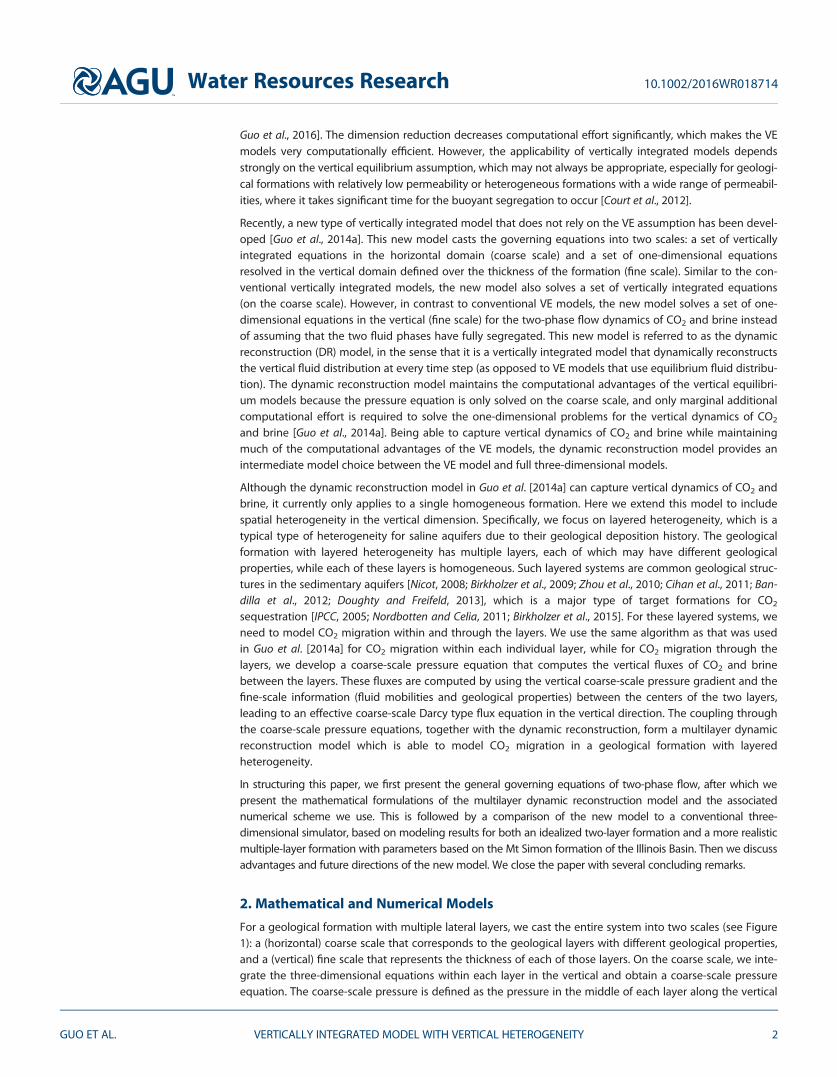
For a geological formation with multiple lateral layers, we cast the entire system into two scales (see Figure1): a (horizontal) coarse scale that corresponds to the geological layers with different geological properties,and a (vertical) fine scale that represents the thickness of each of those layers. On the coarse scale, we inte-grate the three-dimensional equations within each layer in the vertical and obtain a coarse-scale pressureequation. The coarse-scale pressure is defined as the pressure in the middle of each layer along the vertical

Water Resources Research 10.1002/2016WR018714


direction. To couple all the layers, we develop a multilayer coarse-scale pressure equation that couples thecoarse-scale pressure equation at each layer. On the fine scale, we solve the transport equation for the fine-scale saturation and pressure along the vertical columns with the dynamic reconstruction algorithm in Guoet al. [2014a]. In the following subsections, we derive the multilayer coarse-scale pressure equation for thecoarse-scale layers and briefly review the fine-scale dynamic reconstruction algorithm. Following that, wepresent the numerical schemes to solve this multiscale framework.

2.1. Full Three-Dimensional EquationsWe treat the CO2 injection system as a two-phase flow problem, neglecting mutual miscibility between thetwo fluid phases. Note that the multiscale framework in this paper in principle can be extended to include com-ponent transport although we have not explored it in detail. We assume immiscibility between the two fluidphases, in part because the mutual solubility between CO2 and brine is small, up to a few percent [Nordbottenand Celia, 2011], and also because this paper focuses on the CO2 injection period which has a time scale that isshort relative to the time scale for convective mixing of CO2 and brine due to CO2 dissolution [Emami-Meybodiet al., 2015]. Before proceeding to the multiscale algorithms, we first go through the full three-dimensionalequations for two-phase flow in porous media as a basis for the development of the multiscale equations.

The general governing equations for two-phase flow in porous media consist of a mass balance equation and anequation of the extended Darcy’s law for each of the fluid phases, as shown in equations (1) and (2), respectively

@

@tðqa/saÞ1r � ðqauaÞ5qaw

a; (1)

where a5b or c, representing the fluid phase of brine (b) or CO2 (c), qa is fluid density, sa is phase saturation,/ is porosity of the geological porous media, ua is the volumetric Darcy velocity, and wa is a source term (orsink term if negative).

Figure 1. Schematic of the multiscale multilayer dynamic reconstruction algorithm, with three layers as an example. The fine-scale col-umns belong to the coarse-scale layer, and here we take the columns of the second layer (Z2) as an example. The arrows in the columnsrepresent the fluxes from layer Z2 to layer Z3 and from layer Z1 to layer Z2 at the layer boundaries.



ua52kr;aklaðrpa2qagÞ; (2)

where kr;a is relative permeability, k is the permeability tensor of the geological formation, la is viscosity, pa

is phase pressure, and g is gravity acceleration. The relative permeability kr;a is commonly parameterized asa function of phase saturation, that is, kr;a5kr;aðsaÞ. The two phase pressures are related by the capillarypressure, which is also usually taken as an empirical function of phase saturation

pc2pb5pcapðsaÞ: (3)

Finally, the pore space has to be filled up with the two fluid phases, so the phase saturations should sum tounity

sb1sc51: (4)

2.2. Pressure Equation of the Coupled Layers—Coarse ScaleIn a multilayer geological formation, the layers are hydraulically connected. Therefore, the coarse-scale indi-vidual layer should be coupled with the neighbor layers. That is, the coarse-scale pressure equation will bethree-dimensional, where the coarse-scale vertical dimension represents the number of coarse-scale layers.We proceed to derive the coarse-scale pressure equation in two steps. First, we write a vertically integratedmass balance equation for each layer; then we derive an equation for the total fluxes between the layersthat couples the coarse-scale pressures of the two layers. The end result is a multilayer pressure equationthat couples coarse-scale pressures in the entire formation. Details of the standard procedure of verticalintegration for two-phase flow equations can be found in the literature [e.g., Nordbotten and Dahle, 2011;Nordbotten and Celia, 2011; Gasda et al., 2012]. An integration procedure with respect to general pressureprofiles (without assuming vertical equilibrium of the fluid phases) can be found in Guo et al. [2014a].

Following Guo et al. [2014a], the pressure profile in an individual layer can be represented as a referencepressure plus the deviation from the reference pressure, shown in equation (5)

paðx; y; z; tÞ5Paðx; y; tÞ1paðx; y; z; tÞ; (5)

where paðx; y; z; tÞ is the fine-scale phase pressure at point (x, y, z) and Paðx; y; tÞ is the coarse-scale pressure,which we define as the local fine-scale pressure at a reference point in z direction, and paðx; y; z; tÞ is thedeviation of the fine-scale phase pressure at (x, y, z) from the reference pressure. The definition of thecoarse-scale pressure Paðx; y; tÞ leads to a coarse-scale capillary pressure Pcap defined as the local fine-scalecapillary pressure at the reference point. The axis of (x, y) is chosen to be in the plane of the general lateraldirection of the formation, and the z axis is the direction orthogonal to the (x, y) axis (assuming upward pos-itive). Note that the reference pressure can be chosen at any point along the z direction. Here we choosethe reference pressure to be in the center of the layer (along the z axis).

Integrating equation (1) in the z direction from z5fB (bottom of the layer) to z5fT (top of the layer) andsumming over the two fluid phases, we obtain [Guo et al., 2014a]

ðc/H1cbUÞSb@Pb

@t1ðc/H1ccUÞSc

@Pc

@t1rk � ðUb1UcÞ5Wb1Wc2utot;zjfT

1utot;zjfB; (6)

where H is the thickness of the geological layer; c/, cb, and cc are the compressibility coefficients (assumedto be constants) of the porous medium, brine, and CO2, respectively; the ‘‘parallel to’’ subscript k representsthe (x, y) plane and rk5 @

@x ex1 @@y ey , where ex and ey are unit vectors in x and y direction; utot;zjfT

andutot;zjfB

denote the total fluxes (sum of the CO2 and brine fluxes) at the top and the bottom of the layer,respectively; the vertically integrated saturations are defined as Sa51=U

Ð fT

fB/sa dz with U5

Ð fT

fB/ dz; and

Wa is the vertically integrated source term of phase a. The vertically integrated horizontal fluxes havethe following expressions:

Ua52KkKa � ðrkPa2qaGÞ2ðfT

fB

kkkarkpa dz; (7)

where G5ek � g1ðg � ezÞrkfB and ek5ðex; eyÞT ; Kk5Ð fT

fBkk dz; ka5

kr;a

lais the mobility of fluid phase a; Ka5

Kk21Ð fT

fBkkka dz is the vertically integrated mobility of fluid phase a.



The total fluxes at the top (utot;zjfT) and the bottom (utot;z jfB

) in equation (6) are zero in the single-layerdynamic reconstruction model in Guo et al. [2014a]. Thus, equations (6) and (7) give a complete coarse-scale pressure equation for a single-layer system (the functions paðx; y; z; tÞ will be computed on the finescale in section 2.3). However, for a multilayer system, the layers are coupled and utot;zjfT

and utot;zjfBare

nonzero. We need to derive a coarse-scale equation for utot;zjfTand utot;z jfB

that couples the neighbor layers.Without loss of generality, we take the flux between layer j and layer j 1 1 as an example (see Figure 2).Note that we choose the coarse-scale brine pressure Pb as the primary variable for pressure (Pc5Pb1Pcap).We approximate the total flux between the two layers as

utot;j11=252Kz;j11=2Ktot;j11=2Pb;j112Pb;j

DZ1X1;j11=21X2;j11=2

� �; (8)

where Kz;j11=2 and Ktot;j11=2 are the effective coarse-scale permeability and total mobility, respectively,between the two layers; X1;j11=2 and X2;j11=2 are terms associated with capillary pressure and gravity,respectively; DZ5Zj112Zj with Zj and Zj11 the z values of the centers of layer j and j 1 1, respectively; Pb;j

and Pb;j11 are the coarse-scale brine pressures defined as the brine pressure at Z5Zj and Z5Zj11,respectively.

The coefficients Kz;j11=2; Ktot;j11=2, X1;j11=2, and X2;j11=2 are defined based on the fine-scale equations forthe two fluid phase fluxes in the vertical direction, which can be written as

ub;z52kzkb@pb

@z1qbg

� �; (9a)

uc;z52kzkc@pc

@z1qcg

� �: (9b)

Summing equations (9a) and (9b), we obtain the equation for total flux

utot;z52kzðkb1kcÞ@pb

@z2kzkc

@pcap

@z2kzðkbqb1kcqcÞg: (10)

Rearranging equation (10) gives

@pb

@z52

utot;z

kðkb1kcÞ2

kc

kb1kc

@pcap

@z2ðkbqb1kcqcÞ

kb1kcg: (11)

Integrating equation (11) from Zj to Zj11 with respect to z yields

ðZj11

Zj

@pb

@zdz52

ðZj11

Zj

utot;z

kzðkb1kcÞdz2

ðZj11

Zj

kc

kb1kc

@pcap

@zdz2

ðZj11

Zj

ðkbqb1kcqcÞkb1kc

g dz: (12)

The left-side term can be written as ðZj11

Zj

@pb

@zdz5Pb;j112Pb;j : (13)

To derive the coefficients in equation (8), we take utot;Zj11=2as an approximation for the average total flux

from Zj to Zj11 in z direction and obtainðZj11

Zj

utot;z

kzðkb1kcÞdz � utot;Zj11=2

ðZj11

Zj

1kzðkb1kcÞ

dz: (14)

We note that here we approximate utot;Zj11=2as the average total flux from Zj to Zj11 only to derive the coeffi-

cient for equation (8). The actual distribution of total fluxes from Zj to Zj11 will be computed later in thedynamic reconstruction step as outlined in section 2.3 and presented in detail in Appendix A.

Substituting equations (13) and (14) into equation (12) and after some rearrangement, we obtain



utot;Zj11=252

11

DZ

Ð Zj11

Zj

1kzðkb1kcÞ

dz

Pb;j112Pb;j

DZ1

1DZ

ðZj11

Zj

kc

kb1kc

@pcap

@zdz1

1DZ

ðZj11

Zj

ðkbqb1kcqcÞkb1kc

g dz

" #: (15)

Comparing to equation (8), we obtain

Kz;j11=2Ktot;j11=251

1DZ

Ð Zj11

Zj

1kzðkb1kcÞdz

; (16a)

X1;j11=251

DZ

ðZj11

Zj

kc

kb1kc

@pcap

@zdz; (16b)

X2;j11=251

DZ

ðZj11

Zj

ðkbqb1kcqcÞkb1kc

g dz: (16c)

Note that the derived coarse-scale vertical transmissivity Kz;j11=2Ktot;j11=2 between layer j and j 1 1 is a har-monic average of the fine-scale vertical transmissivities, which is consistent with the classic average schemeof vertical hydraulic conductivities.

Similarly, we can obtain the flux between layer j – 1 and j, utot;Zj21=2. Then substituting the two fluxes utot;Zj21=2

and utot;Zj11=2into equation (6), we obtain the coarse-scale pressure equation that couples the neighbor

layers j – 1, j and j 1 1.

ðc/Hj1cbUjSb;j1ccUj Sc;jÞ@Pb;j

@t1ðc/Hj1ccUjÞSc;j

@Pcapj

@t

1rk � 2Kk;jðKb;j1Kc;jÞrkPb;j1Kk;jðqbKb;j1qcKc;jÞGj2Kk;jKc;jrPcapj 2

ðfj11

fj

kkðkbrkpb1kcrkpcÞdz

!

5Kz;j11=2Ktot;j11=2Pb;j112Pb;j

DZ1X1;j11=21X2;j11=2

� �

2Kz;j21=2Ktot;j21=2Pb;j2Pb;j21

DZ1X1;j21=21X2;j21=2

� �1Wb

j 1Wcj :

(17)

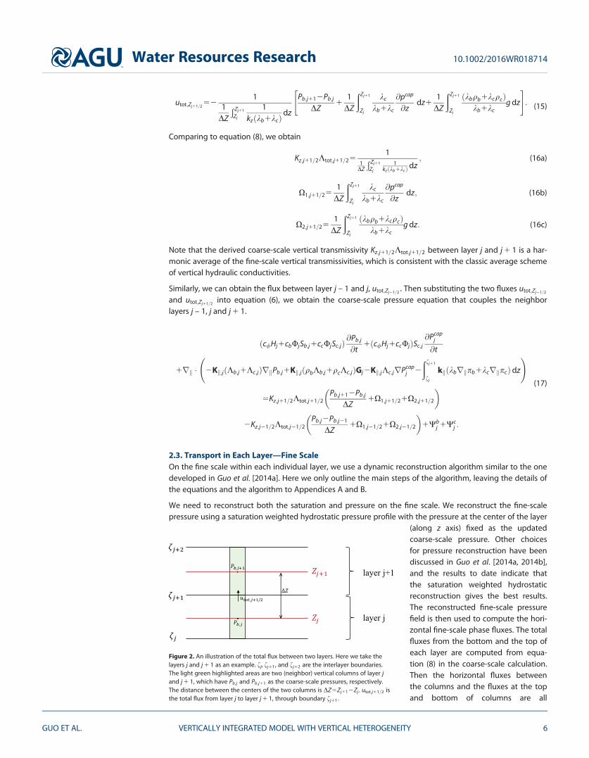
2.3. Transport in Each Layer—Fine ScaleOn the fine scale within each individual layer, we use a dynamic reconstruction algorithm similar to the onedeveloped in Guo et al. [2014a]. Here we only outline the main steps of the algorithm, leaving the details ofthe equations and the algorithm to Appendices A and B.

We need to reconstruct both the saturation and pressure on the fine scale. We reconstruct the fine-scalepressure using a saturation weighted hydrostatic pressure profile with the pressure at the center of the layer

(along z axis) fixed as the updatedcoarse-scale pressure. Other choicesfor pressure reconstruction have beendiscussed in Guo et al. [2014a, 2014b],and the results to date indicate thatthe saturation weighted hydrostaticreconstruction gives the best results.The reconstructed fine-scale pressurefield is then used to compute the hori-zontal fine-scale phase fluxes. The totalfluxes from the bottom and the top ofeach layer are computed from equa-tion (8) in the coarse-scale calculation.Then the horizontal fluxes betweenthe columns and the fluxes at the topand bottom of columns are all

Figure 2. An illustration of the total flux between two layers. Here we take thelayers j and j 1 1 as an example. fj, fj11, and fj12 are the interlayer boundaries.The light green highlighted areas are two (neighbor) vertical columns of layer jand j 1 1, which have Pb;j and Pb;j11 as the coarse-scale pressures, respectively.The distance between the centers of the two columns is DZ5Zj112Zj . utot;j11=2 isthe total flux from layer j to layer j 1 1, through boundary fj11.



computed, and we only need to solve the vertical columns (see Figure 1) as independent one-dimensionalproblems. These one-dimensional problems have ‘‘counter-current’’ type of flow involving buoyancy-drivenupward migration of CO2 and gravity-driven downward drainage of brine, which we solve with a fractionalflow formulation as shown in equations (18a) and (18b). See Appendix A for details of the equations. Notethat the total fluxes utot;z are nonzero; they are computed from the fine-scale horizontal total fluxes and thetotal fluxes at the top and the bottom of the layer. From the fine-scale phase fluxes computed from the frac-tional flow equations, we then compute and reconstruct the CO2 saturation in each column.

ub;z5fb � utot;z2kzkcDqg1kckz@pcap

@z

� �; (18a)

uc;z5fc � utot;z1kzkbDqg2kbkz@pcap

@z

� �: (18b)

2.4. Numerical Scheme and the MLDR AlgorithmThe set of multiscale equations in sections 2.2 and 2.3 are solved numerically, including the coarse-scalepressure equation (17) and the fine-scale equations outlined in Appendix A. We use an IMPES (implicit pres-sure explicit saturation) type method for time stepping and a finite volume method for spatial discretiza-tion. The (coarse-scale) pressure is solved implicitly and the (fine-scale) transport is solved explicitly. Thetwo scales are coupled sequentially (see Figure 1). See Appendix B for details of the numerical discretizationand the computing procedure for the MLDR algorithm.

3. Model Comparison

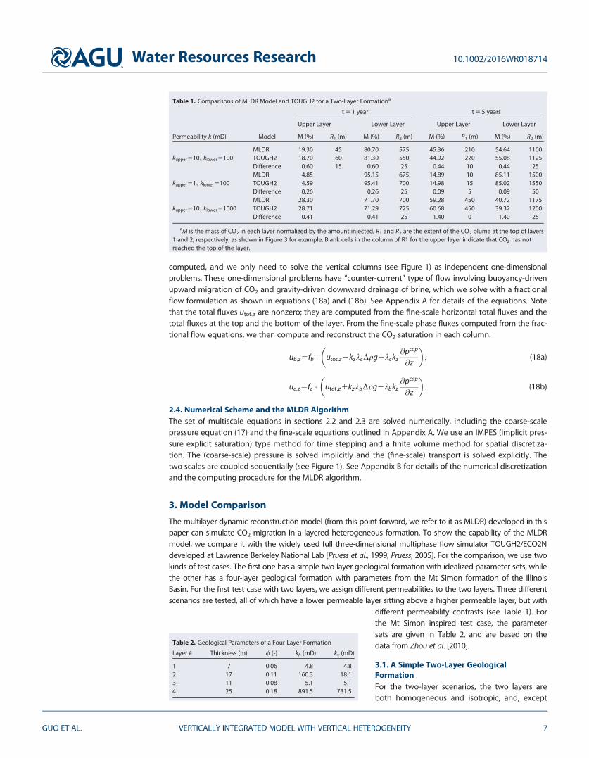
The multilayer dynamic reconstruction model (from this point forward, we refer to it as MLDR) developed in thispaper can simulate CO2 migration in a layered heterogeneous formation. To show the capability of the MLDRmodel, we compare it with the widely used full three-dimensional multiphase flow simulator TOUGH2/ECO2Ndeveloped at Lawrence Berkeley National Lab [Pruess et al., 1999; Pruess, 2005]. For the comparison, we use twokinds of test cases. The first one has a simple two-layer geological formation with idealized parameter sets, whilethe other has a four-layer geological formation with parameters from the Mt Simon formation of the IllinoisBasin. For the first test case with two layers, we assign different permeabilities to the two layers. Three differentscenarios are tested, all of which have a lower permeable layer sitting above a higher permeable layer, but with

different permeability contrasts (see Table 1). Forthe Mt Simon inspired test case, the parametersets are given in Table 2, and are based on thedata from Zhou et al. [2010].

3.1. A Simple Two-Layer GeologicalFormationFor the two-layer scenarios, the two layers areboth homogeneous and isotropic, and, except

Table 1. Comparisons of MLDR Model and TOUGH2 for a Two-Layer Formationa

Permeability k (mD) Model

t 5 1 year t 5 5 years

Upper Layer Lower Layer Upper Layer Lower Layer

M (%) R1 (m) M (%) R2 (m) M (%) R1 (m) M (%) R2 (m)

MLDR 19.30 45 80.70 575 45.36 210 54.64 1100kupper510; klower5100 TOUGH2 18.70 60 81.30 550 44.92 220 55.08 1125

Difference 0.60 15 0.60 25 0.44 10 0.44 25MLDR 4.85 95.15 675 14.89 10 85.11 1500

kupper51; klower5100 TOUGH2 4.59 95.41 700 14.98 15 85.02 1550Difference 0.26 0.26 25 0.09 5 0.09 50MLDR 28.30 71.70 700 59.28 450 40.72 1175

kupper510; klower51000 TOUGH2 28.71 71.29 725 60.68 450 39.32 1200Difference 0.41 0.41 25 1.40 0 1.40 25

aM is the mass of CO2 in each layer normalized by the amount injected, R1 and R2 are the extent of the CO2 plume at the top of layers1 and 2, respectively, as shown in Figure 3 for example. Blank cells in the column of R1 for the upper layer indicate that CO2 has notreached the top of the layer.

Table 2. Geological Parameters of a Four-Layer Formation

Layer # Thickness (m) / (-) kh (mD) kv (mD)

1 7 0.06 4.8 4.82 17 0.11 160.3 18.13 11 0.08 5.1 5.14 25 0.18 891.5 731.5



for different permeabilities, all other parameters are kept the same for the three scenarios. The pairs of per-meabilities for the two layers are (10 mD; 100 mD), (1 mD; 100 mD), and (10 mD, 1000 mD), respectively.Porosity is 0.25 and the system is isothermal with a temperature fixed at 358C. Density and viscosity of thetwo fluid phases are fixed as constants in the MLDR model, while TOUGH2 has an equation of state to com-pute fluid properties from temperature and pressure. For all scenarios, the viscosity and density values usedin MLDR for brine are 7:2031024 Pa s and 1000 kg/m3. The viscosity and density values used for CO2 are7:2631025 Pa s and 810 kg/m3 for the first two scenarios (10 mD; 100 mD), (1 mD; 100 mD), and 6:383

1025 Pa s and 756 kg/m3 for the third scenario (10 mD; 1000 mD). These values were chosen because theycorrespond most closely to the values used in TOUGH2, thereby allowing for a proper comparison of thenumerical solutions. The CO2 injection rate is 1:0 Mt=yearð5109 kg=yearÞ, and CO2 is injected from a verticalwell over the entire thickness of the bottom layer. A boundary condition of hydrostatic pressures is used inthe far field of the domain and the formation is initially saturated with brine. Taking advantage of the sym-metry of the domain, we choose a quarter domain with an injection rate of 0:25 Mt=year to run the models.We use the van Genuchten model to parameterize relative permeability and capillary pressure, with thecharacteristic capillary pressure a21510 Pa and the van Genuchten parameter m5121=n50:99 (n is a mea-sure of the pore-size distribution, n> 1). Note that we have used other sets of van Genuchten parameters,including smaller values of m (e.g., m 5 0.41 adopted from Zhou et al. [2010]), and different m values andentry pressures for different layers. The MLDR model can deal with all these parameter sets and producereasonable results, while the version of TOUGH2 we use runs very slowly for some of the parameter sets.Thus, we only present comparison results for m 5 0.99 and a21510 Pa. To show that the MLDR can dealwith more reasonable parameter sets, we present a set of additional results from MLDR at the end of section3.1. The residual saturation for brine is srb50:3 for both layers. Because we only simulate CO2 injection, thedisplacements only involve drainage, so CO2 residual saturations are not relevant. The entire formation hasa thickness of 50 m and each layer is 25 m thick. The top of the formation has a depth of 1000 m. The hori-zontal extent of the quarter domain is 5 km in both x and y directions. The numerical resolution in the verti-cal is uniform with Dz51 m and the grid size in the horizontal progressively increases from Dx5Dy55 mclose to the injection well to Dx5Dy5100 m at the boundary. The number of numerical grid cells is 120 inboth x and y directions.

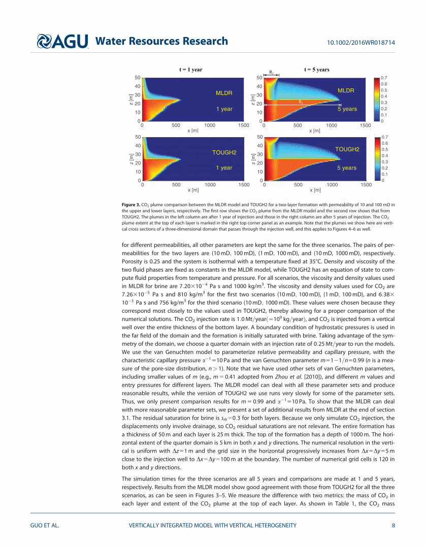
The simulation times for the three scenarios are all 5 years and comparisons are made at 1 and 5 years,respectively. Results from the MLDR model show good agreement with those from TOUGH2 for all the threescenarios, as can be seen in Figures 3–5. We measure the difference with two metrics: the mass of CO2 ineach layer and extent of the CO2 plume at the top of each layer. As shown in Table 1, the CO2 mass

x [m]0 500 1000 1500

z [m

]

0

10

20

30

40

50

x [m]0 500 1000 1500

z [m

]

0

10

20

30

40

50

00.10.20.30.40.50.60.7

1 year

MLDR

5 years

MLDR

x [m]0 500 1000 1500

z [m

]

0

10

20

30

40

50

1 year

TOUGH2

x [m]0 500 1000 1500

z [m

]

0

10

20

30

40

50

00.10.20.30.40.50.60.7

5 years

TOUGH2

t = 1 year t = 5 yearsR1

R2

Figure 3. CO2 plume comparison between the MLDR model and TOUGH2 for a two-layer formation with permeability of 10 and 100 mD inthe upper and lower layers, respectively. The first row shows the CO2 plume from the MLDR model and the second row shows that fromTOUGH2. The plumes in the left column are after 1 year of injection and those in the right column are after 5 years of injection. The CO2

plume extent at the top of each layer is marked in the right top corner panel as an example. Note that the plumes we show here are verti-cal cross sections of a three-dimensional domain that passes through the injection well, and this applies to Figures 4–6 as well.



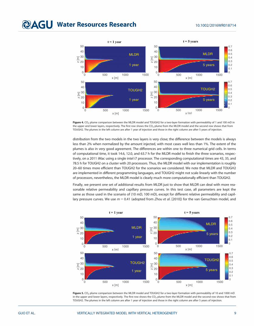
distribution from the two models in the two layers is very close; the difference between the models is alwaysless than 2% when normalized by the amount injected, with most cases well less than 1%. The extent of theplumes is also in very good agreement. The differences are within one to three numerical grid cells. In termsof computational time, it took 14.6, 12.0, and 63.7 h for the MLDR model to finish the three scenarios, respec-tively, on a 2011 iMac using a single intel i7 processor. The corresponding computational times are 43, 35, and78.5 h for TOUGH2 on a cluster with 20 processors. Thus, the MLDR model with our implementation is roughly20–60 times more efficient than TOUGH2 for the scenarios we considered. We note that MLDR and TOUGH2are implemented in different programming languages, and TOUGH2 might not scale linearly with the numberof processors, nevertheless, the MLDR model is clearly much more computationally efficient than TOUGH2.

Finally, we present one set of additional results from MLDR just to show that MLDR can deal with more rea-sonable relative permeability and capillary pressure curves. In this test case, all parameters are kept thesame as those used in the scenario of (10 mD, 100 mD), except for different relative permeability and capil-lary pressure curves. We use m 5 0.41 (adopted from Zhou et al. [2010]) for the van Genuchten model, and

x [m]0 500 1000 1500

z [m

]

0

10

20

30

40

50

00.10.20.30.40.50.60.7

x [m]0 500 1000 1500

z [m

]

0

10

20

30

40

50

x [m]0 500 1000 1500

z [m

]

0

10

20

30

40

50

x [m]0 500 1000 1500

z [m

]

0

10

20

30

40

50

00.10.20.30.40.50.60.7

1 year

TOUGH2

1 year

MLDR

5 years

TOUGH2

5 years

MLDR

t = 1 year t = 5 years

Figure 4. CO2 plume comparison between the MLDR model and TOUGH2 for a two-layer formation with permeability of 1 and 100 mD inthe upper and lower layers, respectively. The first row shows the CO2 plume from the MLDR model and the second row shows that fromTOUGH2. The plumes in the left column are after 1 year of injection and those in the right column are after 5 years of injection.

x [m]0 500 1000 1500

z [m

]

0

10

20

30

40

50

00.10.20.30.40.50.60.7

x [m]0 500 1000 1500

z [m

]

0

10

20

30

40

50

x [m]0 500 1000 1500

z [m

]

0

10

20

30

40

50

00.10.20.30.40.50.60.7

5 years

TOUGH2

5 years

MLDR

x [m]0 500 1000 1500

z [m

]

0

10

20

30

40

50

1 year

TOUGH2

1 year

MLDR


Figure 5. CO2 plume comparison between the MLDR model and TOUGH2 for a two-layer formation with permeability of 10 and 1000 mDin the upper and lower layers, respectively. The first row shows the CO2 plume from the MLDR model and the second row shows that fromTOUGH2. The plumes in the left column are after 1 year of injection and those in the right column are after 5 years of injection.



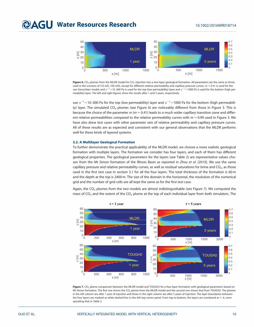
use a21510; 000 Pa for the top (low permeability) layer and a2151000 Pa for the bottom (high permeabili-ty) layer. The simulated CO2 plumes (see Figure 6) are noticeably different from those in Figure 3. This isbecause the choice of the parameter m (m 5 0.41) leads to a much wider capillary transition zone and differ-ent relative permeabilities compared to the relative permeability curves with m 5 0.99 used in Figure 3. Wehave also done test cases with other parameter sets of relative permeability and capillary pressure curves.All of these results are as expected and consistent with our general observations that the MLDR performswell for these kinds of layered systems.

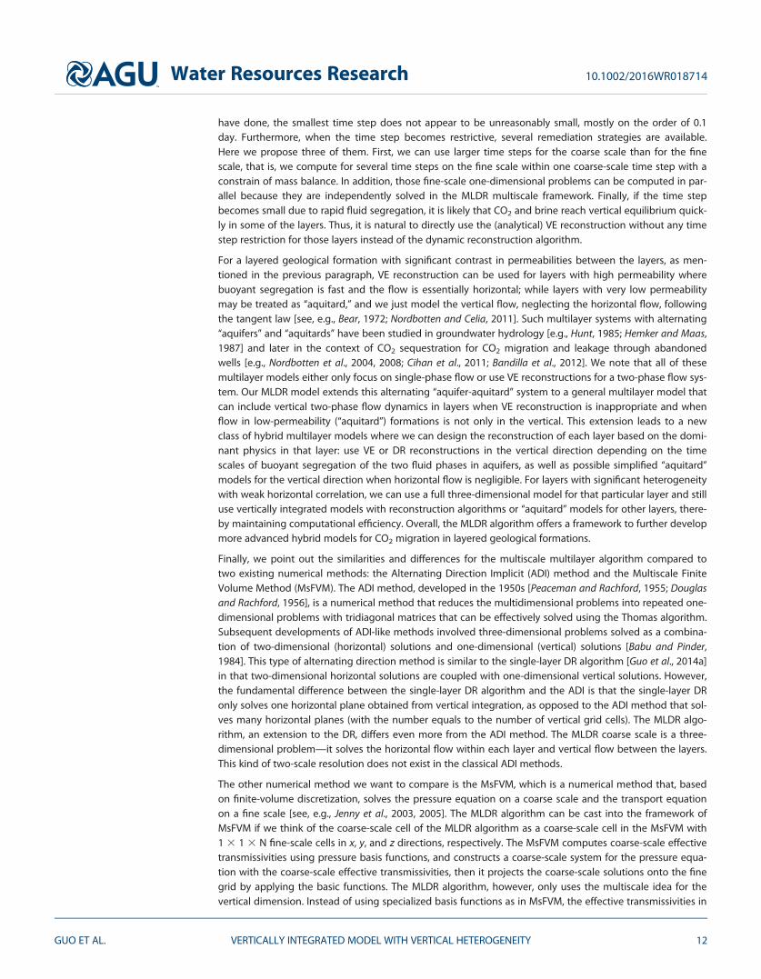
3.2. A Multilayer Geological FormationTo further demonstrate the practical applicability of the MLDR model, we choose a more realistic geologicalformation with multiple layers. The formation we consider has four layers, and each of them has differentgeological properties. The geological parameters for the layers (see Table 2) are representative values cho-sen from the Mt Simon formation of the Illinois Basin as reported in Zhou et al. [2010]. We use the samecapillary pressure and relative permeability curves, as well as residual saturations for brine and CO2, as thoseused in the first test case in section 3.1 for all the four layers. The total thickness of the formation is 60 mand the depth at the top is 2400 m. The size of the domain in the horizontal, the resolution of the numericalgrid and the number of grid cells are all kept the same as for the first test case.

Again, the CO2 plumes from the two models are almost indistinguishable (see Figure 7). We computed themass of CO2 and the extent of the CO2 plume at the top of each individual layer from both simulators. The

0 500 1000 1500x [m]

0

10

20

30

40

50

z [m

]

00.10.20.30.40.50.60.7

0 500 1000 1500x [m]

0

10

20

30

40

50

z [m

]

1 year 5 years

MLDR MLDR

Figure 6. CO2 plumes from the MLDR model for CO2 injection into a two-layer geological formation. All parameters are the same as thoseused in the scenario of (10 mD, 100 mD), except for different relative permeability and capillary pressure curves. m 5 0.41 is used for thevan Genuchten model, and a21510; 000 Pa is used for the top (low permeability) layer and a2151000 Pa is used for the bottom (high per-meability) layer. The left and right figures show the results after 1 and 5 years, respectively.

x [m]0 500 1000 1500 2000

z [m

]

0

10

20

30

40

50

60

00.10.20.30.40.50.60.7

x [m]0 500 1000 1500 2000

z [m

]

0

10

20

30

40

50

60

00.10.20.30.40.50.60.7

x [m]0 200 400 600 800 1000

z [m

]

0102030405060

x [m]0 200 400 600 800 1000

z [m

]

0102030405060

5 years

TOUGH2

5 years

MLDR

1 year

TOUGH2

1 year

MLDR


Figure 7. CO2 plume comparison between the MLDR model and TOUGH2 for a four-layer formation with geological parameters based onMt Simon formation. The first row shows the CO2 plume from the MLDR model and the second row shows that from TOUGH2. The plumesin the left column are after 1 year of injection and those in the right column are after 5 years of injection. The layer boundaries betweenthe four layers are marked as white dashed line in the left-top corner panel. From top to bottom, the layers are numbered as 1–4, corre-sponding that in Table 2.



difference is very small (see Table 3), asis expected from the good visual agree-ment of the CO2 plumes in Figure 7.The maximum difference of CO2 mass isless than 1% of the total mass injected,and the difference of the CO2 plumeextent is all within one grid cell. Interms of computational time, the MLDRsimulator used about 50 h on a 2011iMac using a single intel i7 processor,while it took more than 200 h forTOUGH2 to finish the simulation on acluster with 10 processors.

Finally, we note that the implementa-tion of the MLDR model assumes con-stant density and viscosity of the two

fluids. The density we used in the simulation shown herein is the saturation weighted density from resultsof the TOUGH2 simulations, and the viscosity is computed from the pressure corresponding to the comput-ed saturation weighted density. The viscosity and density values used in MLDR for brine are 7:2031024 Pa sand 1000 kg/m3, and for CO2 are 6:3331025 Pa s and 752 kg/m3. Despite the assumption of constant densi-ty and viscosity in the MLDR model, the predictions of CO2 plumes are in very good agreement with thosefrom TOUGH2. This is because the density and viscosity do not have much variation in the test cases weconsidered and therefore it is reasonable to assume constant density and viscosity. In fact, a simple estima-tion of density and viscosity from the initial pressure in the formation (before CO2 is injected) is very closeto what we got from the TOUGH2 simulation. Nevertheless, for geological formations where variations indensity and viscosity are important, an equation of state needs to be implemented for each of the fluidphases in the MLDR model.

4. Discussion

The MLDR model captures the vertical dynamics of CO2 and brine well both within each individual layerand between the layers. All comparisons of MLDR and TOUGH2 show excellent results. Further, the MLDRalgorithm significantly reduces computational effort compared to full three-dimensional models. In theMLDR model, pressures are only solved on the coarse scale. The size of the matrix to solve the pressureequation is significantly reduced compared to a full three-dimensional model, where all the fine-scale pres-sures needed to be solved. Also, the remaining fine-scale one-dimensional ‘‘counter-current’’ flow problemis easy to solve using the fractional flow formulation. Thus, the multilayer dynamic reconstruction algorithmleads to significant reduction of computational effort. Here we take a geological formation with three layersas an example and give a simple analysis of the complexity of the algorithm. The pressure solver of theMLDR model has a complexity of OðN2

x 3N2y 332Þ, while the full three-dimensional model has a complexity

of OðN2x 3N2

y 3ðNz11Nz21Nz3Þ2Þ. Nx and Ny are the number of grid cells in x and y directions, respectively.Nz1; Nz2, and Nz3 are the numbers of vertical grid cells in each of the three layers. This simple analysis showsthat the MLDR algorithm reduces the computational cost by an order of OððNz=3Þ2Þ, where Nz5Nz11Nz21

Nz3 is the total number of numerical grids in z direction. It should be noted that the pressure solution is themost computationally intensive part of both the MLDR and conventional three-dimensional algorithms.Although we recognize that TOUGH2 may be slowed partially by the additional computation of componenttransport and inclusion of compressibility, for the simulations presented here, despite that the implementa-tion of the MLDR is not much optimized, the MLDR model is at least 20 times more computationally effi-cient compared to TOUGH2; it is 40–60 times faster for most of the simulations we have analyzed. We notethat here the comparison of computational efficiency is made by assuming that the processors that MLDRand TOUGH2 use have similar speed and TOUGH2 scales linearly with the number of processors.

The MLDR model uses an explicit scheme for the fine-scale one-dimensional problem; it may require smalltime steps when the CO2 and brine segregate rapidly in the vertical. Nevertheless, in the simulations we

Table 3. Comparisons of MLDR Model and TOUGH2 for a Four-LayerFormationa

Layer # Model

t 5 1 year t 5 5 years

M (%) R (m) M (%) R (m)

MLDR 0.21 80 10.92 11001 TOUGH2 0.22 80 11.05 1125

Difference 0.01 0 0.13 25MLDR 2.75 140 21.83 1225

2 TOUGH2 2.55 140 21.98 1250Difference 0.20 0 0.15 25MLDR 22.71 450 20.21 1350

3 TOUGH2 23.03 450 20.83 1375Difference 0.32 0 0.62 25MLDR 74.33 875 47.04 1450

4 TOUGH2 74.20 875 46.13 1475Difference 0.13 0 0.91 25

aM is the mass of CO2 in each layer normalized by the amount injected, R isthe extent of the CO2 plume at the top of each layer.



have done, the smallest time step does not appear to be unreasonably small, mostly on the order of 0.1day. Furthermore, when the time step becomes restrictive, several remediation strategies are available.Here we propose three of them. First, we can use larger time steps for the coarse scale than for the finescale, that is, we compute for several time steps on the fine scale within one coarse-scale time step with aconstrain of mass balance. In addition, those fine-scale one-dimensional problems can be computed in par-allel because they are independently solved in the MLDR multiscale framework. Finally, if the time stepbecomes small due to rapid fluid segregation, it is likely that CO2 and brine reach vertical equilibrium quick-ly in some of the layers. Thus, it is natural to directly use the (analytical) VE reconstruction without any timestep restriction for those layers instead of the dynamic reconstruction algorithm.

For a layered geological formation with significant contrast in permeabilities between the layers, as men-tioned in the previous paragraph, VE reconstruction can be used for layers with high permeability wherebuoyant segregation is fast and the flow is essentially horizontal; while layers with very low permeabilitymay be treated as ‘‘aquitard,’’ and we just model the vertical flow, neglecting the horizontal flow, followingthe tangent law [see, e.g., Bear, 1972; Nordbotten and Celia, 2011]. Such multilayer systems with alternating‘‘aquifers’’ and ‘‘aquitards’’ have been studied in groundwater hydrology [e.g., Hunt, 1985; Hemker and Maas,1987] and later in the context of CO2 sequestration for CO2 migration and leakage through abandonedwells [e.g., Nordbotten et al., 2004, 2008; Cihan et al., 2011; Bandilla et al., 2012]. We note that all of thesemultilayer models either only focus on single-phase flow or use VE reconstructions for a two-phase flow sys-tem. Our MLDR model extends this alternating ‘‘aquifer-aquitard’’ system to a general multilayer model thatcan include vertical two-phase flow dynamics in layers when VE reconstruction is inappropriate and whenflow in low-permeability (‘‘aquitard’’) formations is not only in the vertical. This extension leads to a newclass of hybrid multilayer models where we can design the reconstruction of each layer based on the domi-nant physics in that layer: use VE or DR reconstructions in the vertical direction depending on the timescales of buoyant segregation of the two fluid phases in aquifers, as well as possible simplified ‘‘aquitard’’models for the vertical direction when horizontal flow is negligible. For layers with significant heterogeneitywith weak horizontal correlation, we can use a full three-dimensional model for that particular layer and stilluse vertically integrated models with reconstruction algorithms or ‘‘aquitard’’ models for other layers, there-by maintaining computational efficiency. Overall, the MLDR algorithm offers a framework to further developmore advanced hybrid models for CO2 migration in layered geological formations.

Finally, we point out the similarities and differences for the multiscale multilayer algorithm compared totwo existing numerical methods: the Alternating Direction Implicit (ADI) method and the Multiscale FiniteVolume Method (MsFVM). The ADI method, developed in the 1950s [Peaceman and Rachford, 1955; Douglasand Rachford, 1956], is a numerical method that reduces the multidimensional problems into repeated one-dimensional problems with tridiagonal matrices that can be effectively solved using the Thomas algorithm.Subsequent developments of ADI-like methods involved three-dimensional problems solved as a combina-tion of two-dimensional (horizontal) solutions and one-dimensional (vertical) solutions [Babu and Pinder,1984]. This type of alternating direction method is similar to the single-layer DR algorithm [Guo et al., 2014a]in that two-dimensional horizontal solutions are coupled with one-dimensional vertical solutions. However,the fundamental difference between the single-layer DR algorithm and the ADI is that the single-layer DRonly solves one horizontal plane obtained from vertical integration, as opposed to the ADI method that sol-ves many horizontal planes (with the number equals to the number of vertical grid cells). The MLDR algo-rithm, an extension to the DR, differs even more from the ADI method. The MLDR coarse scale is a three-dimensional problem—it solves the horizontal flow within each layer and vertical flow between the layers.This kind of two-scale resolution does not exist in the classical ADI methods.

The other numerical method we want to compare is the MsFVM, which is a numerical method that, basedon finite-volume discretization, solves the pressure equation on a coarse scale and the transport equationon a fine scale [see, e.g., Jenny et al., 2003, 2005]. The MLDR algorithm can be cast into the framework ofMsFVM if we think of the coarse-scale cell of the MLDR algorithm as a coarse-scale cell in the MsFVM with1 3 1 3 N fine-scale cells in x, y, and z directions, respectively. The MsFVM computes coarse-scale effectivetransmissivities using pressure basis functions, and constructs a coarse-scale system for the pressure equa-tion with the coarse-scale effective transmissivities, then it projects the coarse-scale solutions onto the finegrid by applying the basic functions. The MLDR algorithm, however, only uses the multiscale idea for thevertical dimension. Instead of using specialized basis functions as in MsFVM, the effective transmissivities in



MLDR are derived from vertical integration. Thus, although MLDR can be cast into the general MsFVMframework, it is a noval multiscale algorithm developed by using vertical integration and reconstructionoperators.

5. Conclusion

In this paper, we present a multilayer dynamic reconstruction algorithm that can simulate CO2 migration indeep saline aquifers with layered heterogeneity. The algorithm is based on casting the full three-dimensionalgoverning equations into two scales. The coarse scale is the multiple vertically integrated layers, with coarse-scale pressure only a function of (x,y) in any layer, and a coarse-scale pressure equation that couples all thelayers. The fine scale corresponds to the vertical one-dimensional columns defined within the thickness of eachlayer, on which we solve the two-phase flow dynamics of CO2 and brine with the dynamic reconstruction algo-rithm from Guo et al. [2014a]. Results show that the MLDR model is in excellent agreement with a full three-dimensional simulator (TOUGH2) for all the test cases we considered. The MLDR model is also much more com-putationally efficient compared to TOUGH2, with computational time 20–60 times smaller for MLDR.

In summary, the MLDR model is accurate and much more computationally efficient than conventional fullthree-dimensional simulators, and the computational advantages make it an attractive tool for simulationsof CO2 migration in large-scale CO2 sequestration systems. In addition, the MLDR model provides a model-ing framework for CO2 migration in geological formation with layered heterogeneities, which can lead tothe development of a new class of hybrid models where different reconstructions can be chosen for differ-ent layers based on their different time scales of buoyant segregation.

Appendix A: The Fine-Scale Equations

In this appendix section, we outline the fine-scale equations for the transport within each layer. The fine-scale equations are almost identical to those presented in Guo et al. [2014a], except that the vertical fluxesat the top and bottom of the layers are nonzero.

On the fine scale, the mass balance equation can be rearranged to focus on the vertical dynamics

@ qa/sað Þ@t

1@ qaua;z� �@z

5qawa2rk � qaua;k� �

: (A1)

With the assumption of ‘‘slight compressibility’’ used in Guo et al. [2014a], equation (A1) becomes

/@sa

@t1ðc/1/caÞsa

@pa

@t1@ua;3

@x35wa2rk � ua;k; (A2)

where the horizontal fluxes can be computed from equation (A3)

ua;k52kkka � rkpa2qa ek � g� ��

: (A3)

Summing equation (A2) over the two fluid phases, we can calculate the total flux, utot;z , in the z direction,from the horizontal fluxes ua;k and source term wa. Given the total flux values in the z direction, the verticalphase flux ua;z can be computed using the fractional flow form of Darcy’s law (equations (18a) and (18b))

ub;z5fb � utot;z2kzkcDqg1kckz@pcap

@z

� �; (A4a)

uc;z5fc � utot;z1kzkbDqg2kbkz@pcap

@z

� �; (A4b)

where kz is permeability in z direction, and fa is the fractional flow function, given by

fa5ka

kb1kc: (A5)

Substituting equations (A4a) and (A4b) into equation (A2), we can compute saturations for each fluidphase.



Now given the fine-scale saturations, we can analytically reconstruct the profiles of phase pressures in zdirection. We reconstruct the fine-scale pressure using a saturation weighted hydrostatic pressure profile asshown in equations (A6a) and (A6b)

@pc

@z52ðscqc1sbqbÞg1sb

@pcapðsbÞ@z

; (A6a)

@pb

@z52ðscqc1sbqbÞg2sc

@pcapðsbÞ@z

: (A6b)

From equations (A6a) and (A6b), the function pa in equation (5) can be derived, which gives a fine-scalepressure profile from the coarse-scale pressure. For example, when a5b, integration from the bottom of theformation yields

pbðx; y; z; tÞ5Pbðx; y; tÞ2ðz

fB

ðscqc1sbqbÞg1sc@pcapðsbÞ

@z

� dz: (A7)

To this point, the fine-scale saturation and pressure profiles are both reconstructed. We can proceed tosolve the coarse-scale variables (Pb and Pc) for the next time step. In the following Appendix B, we will out-line the numerical scheme to solve the coarse-scale and fine-scale equations, and the step-by-step MLDRalgorithm.

Appendix B: Numerical Scheme and the MLDR Algorithm

A time stepping scheme analogous to the implicit pressure-explicit saturation (IMPES) method is used inthis paper. We solve pressure on the coarse scale (multiple vertically integrated layers) implicitly, while solvethe saturation on the fine scale explicitly. Equation (B1) shows the time discretization of the coarse-scalepressure equation. We linearize the equation by lagging one time step for the coefficients, e.g., mobilitiesand capillary pressure.

ðc/Hj1cbUj Snb;j1ccUj Sn

c;jÞPn11

b;j 2Pnb;j

Dt1ðc/Hj1ccUjÞSn

c;j

Pcap;nj 2Pcap;n21

j

Dt

1rk � 2Kk;jðKnb;j1Kn

c;jÞrkPn11b;j 1Kk;jðqbK

nb;j1qcK

nc;jÞGj2Kk;jK

nc;jrPcap;n

j 2

ðfj11

fj

kk;jðknbrkpn

b1kncrkpn

c Þdz

!

5Kz;j11=2Kntot;j11=2

Pn11b;j112Pn11

b;j

DZ1Xn

1;j11=21Xn2;j11=2

!

2Kz;j21=2Kntot;j21=2

Pn11b;j 2Pn11

b;j21

DZ1Xn

1;j21=21Xn2;j21=2

!1Wb;n11

j 1Wc;n11j :

(B1)

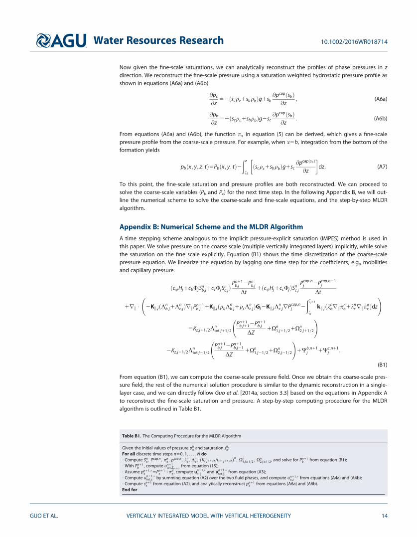
From equation (B1), we can compute the coarse-scale pressure field. Once we obtain the coarse-scale pres-sure field, the rest of the numerical solution procedure is similar to the dynamic reconstruction in a single-layer case, and we can directly follow Guo et al. [2014a, section 3.3] based on the equations in Appendix Ato reconstruct the fine-scale saturation and pressure. A step-by-step computing procedure for the MLDRalgorithm is outlined in Table B1.

Table B1. The Computing Procedure for the MLDR Algorithm

Given the initial values of pressure p0a and saturation s0

a :For all discrete time steps n50; 1; . . . ;N do- Compute Sn

a ; Pcap;n; pna ; pcap;n; kn

a ; Kna ; Kz;j61=2Ktot;j61=2

� �n; Xn

1;j61=2; Xn2;j61=2, and solve for Pn11

b from equation (B1);- With Pn11

b , compute un11tot;Zj11=2

from equation (15);- Assume pn11;�

a 5Pn11a 1pn

a , compute un11;�a;k and un11;�

tot;k from equation (A3);- Compute un11;�

tot;z by summing equation (A2) over the two fluid phases, and compute un11;�a;z from equations (A4a) and (A4b);

- Compute sn11a from equation (A2), and analytically reconstruct pn11

a from equations (A6a) and (A6b).End for



ReferencesAndersen, O., S. E. Gasda, and H. M. Nilsen (2015), Vertically averaged equations with variable density for CO2 flow in porous media, Transp.

Porous Media, 107(1), 95–127.Babu, D., and G. Pinder (1984), A finite element-finite difference alternating direction algorithm for three dimensional groundwater trans-

port, in Finite Elements in Water Resources, pp. 165–174, Springer, Verlag Berlin Heildelberg.Bandilla, K. W., M. A. Celia, T. R. Elliot, M. Person, K. M. Ellett, J. A. Rupp, C. Gable, and Y. Zhang (2012), Modeling carbon sequestration in the

Illinois basin using a vertically-integrated approach, Comput. Visualization Sci., 15(1), 39–51.Bandilla, K. W., M. A. Celia, J. T. Birkholzer, A. Cihan, and E. C. Leister (2015), Multiphase modeling of geologic carbon sequestration in saline

aquifers, Groundwater, 53(3), 362–377.Bear, J. (1972), Dynamics of Fluids in Porous Media, Elsevier, N. Y.Birkholzer, J. T., Q. Zhou, and C.-F. Tsang (2009), Large-scale impact of CO2 storage in deep saline aquifers: A sensitivity study on pressure

response in stratified systems, Int. J. Greenhouse Gas Control, 3(2), 181–194.Birkholzer, J. T., C. M. Oldenburg, and Q. Zhou (2015), CO2 migration and pressure evolution in deep saline aquifers, Int. J. Greenhouse Gas

Control, 40, 203–220.Celia, M., S. Bachu, J. Nordbotten, and K. Bandilla (2015), Status of CO2 storage in deep saline aquifers with emphasis on modeling

approaches and practical simulations, Water Resour. Res., 51, 6846–6892, doi:10.1002/2015WR017609.Cihan, A., Q. Zhou, and J. T. Birkholzer (2011), Analytical solutions for pressure perturbation and fluid leakage through aquitards and wells

in multilayered-aquifer systems, Water Resour. Res., 47, W10504, doi:10.1029/2011WR010721.Court, B., K. W. Bandilla, M. A. Celia, A. Janzen, M. Dobossy, and J. M. Nordbotten (2012), Applicability of vertical-equilibrium and sharp-

interface assumptions in CO2 sequestration modeling, Int. J. Greenhouse Gas Control, 10, 134–147.Doughty, C., and B. M. Freifeld (2013), Modeling CO2 injection at Cranfield, Mississippi: Investigation of methane and temperature effects,

Greenhouse Gases Sci. Technol., 3(6), 475–490.Douglas, J., and H. H. Rachford (1956), On the numerical solution of heat conduction problems in two and three space variables, Trans. Am.

Math. Soc., 82, 421–439.Emami-Meybodi, H., H. Hassanzadeh, C. P. Green, and J. Ennis-King (2015), Convective dissolution of CO2 in saline aquifers: Progress in

modeling and experiments, Int. J. Greenhouse Gas Control, 40, 238–266.Gasda, S. E., J. M. Nordbotten, and M. A. Celia (2009), Vertical equilibrium with sub-scale analytical methods for geological CO2 sequestra-

tion, Comput. Geosci., 13(4), 469–481.Gasda, S. E., H. M. Nilsen, H. K. Dahle, and W. G. Gray (2012), Effective models for CO2 migration in geological systems with varying topogra-

phy, Water Resour. Res., 48, W10546, doi:10.1029/2012WR012264.Guo, B., K. W. Bandilla, F. Doster, E. Keilegavlen, and M. A. Celia (2014a), A vertically integrated model with vertical dynamics for CO2 stor-

age, Water Resour. Res., 50, 6269–6284, doi:10.1002/2013WR015215.Guo, B., K. W. Bandilla, E. Keilegavlen, F. Doster, and M. A. Celia (2014b), Application of vertically-integrated models with subscale vertical

dynamics to field sites for CO2 sequestration, Energy Proc., 63, 3523–3531.Guo, B., Z. Zheng, M. A. Celia, and H. A. Stone (2016), Axisymmetric flows from fluid injection into a confined porous medium, Phys. Fluids,

28(2).Hemker, C., and C. Maas (1987), Unsteady flow to wells in layered and fissured aquifer systems, J. Hydrol., 90(3), 231–249.Hesse, M., F. Orr, and H. Tchelepi (2008), Gravity currents with residual trapping, J. Fluid Mech., 611, 35–60.Hunt, B. (1985), Flow to a well in a multiaquifer system, Water Resour. Res., 21(11), 1637–1641.Huppert, H. E., and A. W. Woods (1995), Gravity-driven flows in porous layers, J. Fluid Mech., 292, 55–69.IPCC. (2005), IPCC Special Report on Carbon Dioxide Capture and Storage, edited by B. Metz, et al., Cambridge Univ. Press, N. Y.Jenny, P., S. Lee, and H. Tchelepi (2003), Multi-scale finite-volume method for elliptic problems in subsurface flow simulation, J. Comput.

Phys., 187(1), 47–67.Jenny, P., S. Lee, and H. Tchelepi (2005), Adaptive multiscale finite-volume method for multiphase flow and transport in porous media, Mul-

tiscale Model. Simul., 3(1), 50–64.Lake, L. W. (1989), Enhanced Oil Recovery, Prentice Hall, Englewood Cliffs, N. J.Lyle, S., H. E. Huppert, M. Hallworth, M. Bickle, and A. Chadwick (2005), Axisymmetric gravity currents in a porous medium, J. Fluid Mech.,

543, 293–302.MacMinn, C. W., M. L. Szulczewski, and R. Juanes (2010), CO2 migration in saline aquifers. part 1. Capillary trapping under slope and

groundwater flow, J. Fluid Mech., 662, 329–351.Michael, K., A. Golab, V. Shulakova, J. Ennis-King, G. Allinson, S. Sharma, and T. Aiken (2010), Geological storage of CO2 in saline aquifers—A

review of the experience from existing storage operations, Int. J. Greenhouse Gas Control, 4(4), 659–667.Nicot, J.-P. (2008), Evaluation of large-scale CO2 storage on fresh-water sections of aquifers: An example from the Texas gulf coast basin,

Int. J. Greenhouse Gas Control, 2(4), 582–593.Nilsen, H. M., K.-A. Lie, and O. Andersen (2015), Robust simulation of sharp-interface models for fast estimation of CO2 trapping capacity in

large-scale aquifer systems, Comput. Geosci., 20, 1–21.Nordbotten, J. M., and M. A. Celia (2006), Similarity solutions for fluid injection into confined aquifers, J. Fluid Mech., 561,

307–327.Nordbotten, J. M., and M. A. Celia (2011), Geological Storage of CO2: Modeling Approaches for Large-Scale Simulation, John Wiley, Hoboken,

N. J.Nordbotten, J. M., and H. K. Dahle (2011), Impact of the capillary fringe in vertically integrated models for CO2 storage, Water Resour. Res.,

47, W02537, doi:10.1029/2009WR008958.Nordbotten, J. M., M. A. Celia, and S. Bachu (2004), Analytical solutions for leakage rates through abandoned wells, Water Resources

Research, 40, W04204, doi:10.1029/2003WR002997.Nordbotten, J. M., D. Kavetski, M. A. Celia, and S. Bachu (2008), Model for CO2 leakage including multiple geological layers and multiple

leaky wells, Environ. Sci. Technol., 43(3), 743–749.Pacala, S., and R. Socolow (2004), Stabilization wedges: Solving the climate problem for the next 50 years with current technologies,

Science, 305(5686), 968–972.Peaceman, D. W., and H. H. Rachford Jr. (1955), The numerical solution of parabolic and elliptic differential equations, J. Soc. Ind. Appl.

Math., 3(1), 28–41.Pegler, S. S., H. E. Huppert, and J. A. Neufeld (2014), Fluid injection into a confined porous layer, J. Fluid Mech., 745, 592–620.

AcknowledgmentsThis work was supported in part by theNational Science Foundation undergrant EAR-0934722; the Department ofEnergy under grant DE-FE0009563;and the Carbon Mitigation Initiative atPrinceton University. We also thankRainer Helmig from University ofStuttgart for helpful discussions. All ofthe data used in this study arepresented in the paper, includingmodel inputs and outputs.



http://dx.doi.org/10.1002/2015WR017609

http://dx.doi.org/10.1029/2011WR010721

http://dx.doi.org/10.1029/2012WR012264

http://dx.doi.org/10.1002/2013WR015215

http://dx.doi.org/10.1029/2009WR008958

http://dx.doi.org/10.1029/2003WR002997

Pruess, K. (2005), ECO2N: A TOUGH2 Fluid Property Module for Mixtures of Water, NaCl, and CO2, Lawrence Berkeley Natl. Lab., Berkeley, Calif.Pruess, K., C. Oldenburg, and G. Moridis (1999), TOUGH2 User’s Guide Version 2, Lawrence Berkeley Natl. Lab., Berkeley, Calif.Wu, Y.-S., P. Huyakorn, and N. Park (1994), A vertical equilibrium model for assessing nonaqueous phase liquid contamination and remedia-

tion of groundwater systems, Water Resour. Res., 30(4), 903–912.Zheng, Z., B. Guo, I. C. Christov, M. A. Celia, and H. A. Stone (2015), Flow regimes for fluid injection into a confined porous medium, J. Fluid

Mech., 767, 881–909.Zhou, Q., J. T. Birkholzer, E. Mehnert, Y.-F. Lin, and K. Zhang (2010), Modeling basin-and plume-scale processes of CO2 storage for full-scale

deployment, Groundwater, 48(4), 494–514.



Documents

A multiscale multilayer vertically integrated model …boguo/pdfs/publications/2016_Guo_et_al...A multiscale multilayer vertically integrated model with ... 2 sequestration in layered