Embed Size (px)
Citation preview

v
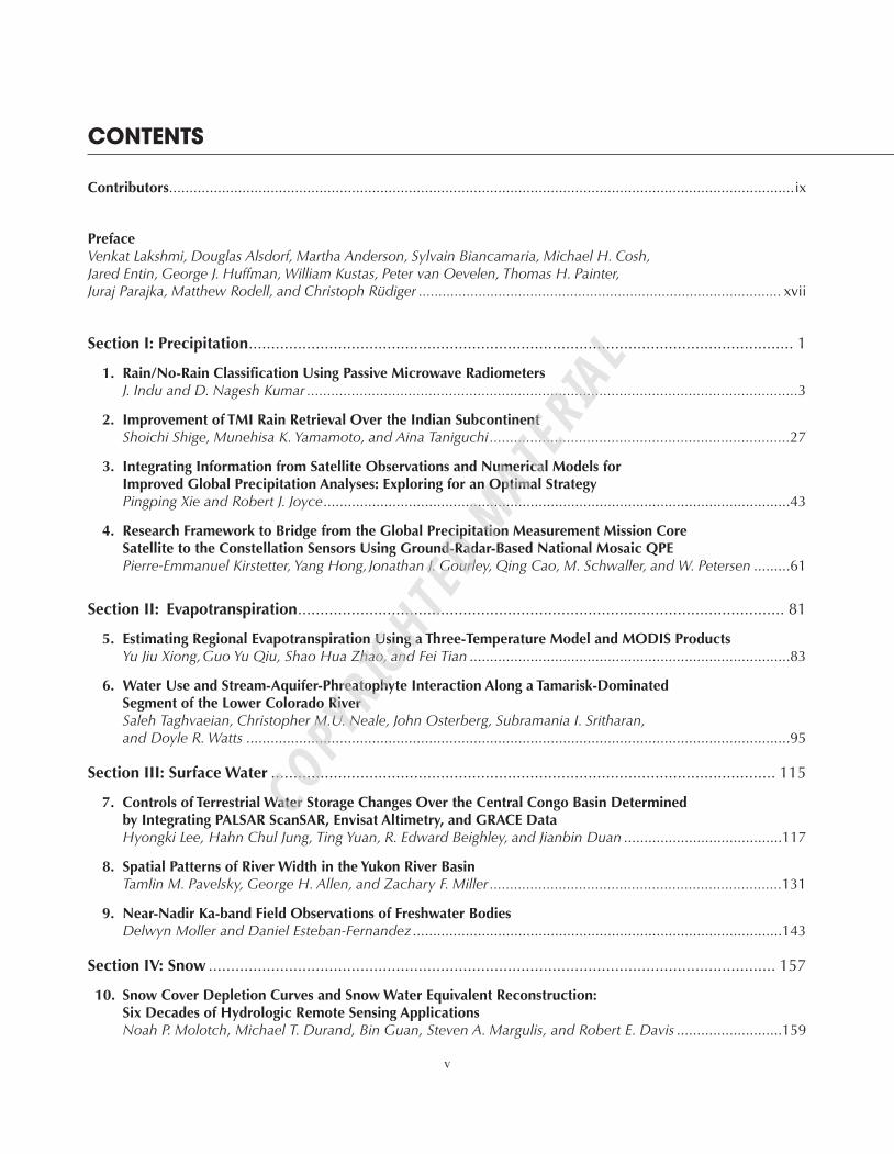
Contents
Contributors ix
PrefaceVenkat Lakshmi, Douglas Alsdorf, Martha Anderson, Sylvain Biancamaria, Michael H. Cosh, Jared Entin, George J. Huffman, William Kustas, Peter van Oevelen, Thomas H. Painter, Juraj Parajka, Matthew Rodell, and Christoph Rüdiger ........................................................................................... xvii
Section I: Precipitation 1
1. Rain/No-Rain Classification Using Passive Microwave RadiometersJ. Indu and D. Nagesh Kumar .........................................................................................................................3
2. Improvement of TMI Rain Retrieval Over the Indian SubcontinentShoichi Shige, Munehisa K. Yamamoto, and Aina Taniguchi ..........................................................................27
3. Integrating Information from Satellite Observations and Numerical Models for Improved Global Precipitation Analyses: Exploring for an Optimal StrategyPingping Xie and Robert J. Joyce 43
4. Research Framework to Bridge from the Global Precipitation Measurement Mission Core Satellite to the Constellation Sensors Using Ground-Radar-Based National Mosaic QPEPierre-Emmanuel Kirstetter, Yang Hong, Jonathan J. Gourley, Qing Cao, M. Schwaller, and W. Petersen 61
Section II: Evapotranspiration 81
5. Estimating Regional Evapotranspiration Using a Three-Temperature Model and MODIS ProductsYu Jiu Xiong, Guo Yu Qiu, Shao Hua Zhao, and Fei Tian 83
6. Water Use and Stream-Aquifer-Phreatophyte Interaction Along a Tamarisk-Dominated Segment of the Lower Colorado RiverSaleh Taghvaeian, Christopher M.U. Neale, John Osterberg, Subramania I. Sritharan, and Doyle R. Watts 95
Section III: Surface Water 115
7. Controls of Terrestrial Water Storage Changes Over the Central Congo Basin Determined by Integrating PALSAR ScanSAR, Envisat Altimetry, and GRACE DataHyongki Lee, Hahn Chul Jung, Ting Yuan, R. Edward Beighley, and Jianbin Duan 117
8. Spatial Patterns of River Width in the Yukon River BasinTamlin M. Pavelsky, George H. Allen, and Zachary F. Miller ........................................................................131
9. Near-Nadir Ka-band Field Observations of Freshwater BodiesDelwyn Moller and Daniel Esteban-Fernandez 143
Section IV: Snow 157
10. Snow Cover Depletion Curves and Snow Water Equivalent Reconstruction: Six Decades of Hydrologic Remote Sensing ApplicationsNoah P. Molotch, Michael T. Durand, Bin Guan, Steven A. Margulis, and Robert E. Davis 159
0002184454.indd 5 10/15/2014 8:47:24 AM
COPYRIG
HTED M
ATERIAL

vi Contents
11. Retrieval and Validation of VIIRS Snow Cover Information for Terrestrial Water Cycle ApplicationsIgor Appel ..................................................................................................................................................175
12. Seeing the Snow Through the Trees: Toward a Validated Canopy Adjustment for Satellite Snow-Covered AreaLexi P. Coons, Anne W. Nolin, Kelly E. Gleason, Eugene J. Mar, Karl Rittger, Travis R. Roth, and Thomas H. Painter 199
13. Passive Microwave Remote Sensing of Snowmelt and Melt-Refreeze Using Diurnal Amplitude VariationsKathryn Alese Semmens, Joan Ramage, Jeremy D. Apgar, Katrina E. Bennett, Glen E. Liston, and Elias Deeb 215
14. Changes in Snowpacks of Canadian Prairies for 1979–2004 Detected from Snow Water Equivalent Data of SMMR and SSM/I Passive Microwave and Related Climatic FactorsThian Yew Gan, Roger G. Barry, and Adam K. Gobena 227
Section V: Soil Moisture 245
15. Some Issues in Validating Satellite-Based Soil Moisture Retrievals from SMAP with in Situ ObservationsThomas J. Jackson, Michael Cosh, and Wade Crow.....................................................................................247
16. Soil Moisture Retrieval from Microwave (RADARSAT-2) and Optical Remote Sensing (MODIS) Data Using Artificial Intelligence TechniquesNasreen Jahan and Thian Yew Gan ............................................................................................................255
17. AMSR-E Soil Moisture Disaggregation Using MODIS and NLDAS DataBin Fang and Venkat Lakshmi .....................................................................................................................277
18. Assessing Near-Surface Soil Moisture Assimilation Impacts on Modeled Root-Zone Moisture for an Australian Agricultural LandscapeR. C. Pipunic, D. Ryu, and J. P. Walker 305
19. Assimilation of Satellite Soil Moisture Retrievals into Hydrologic Model for Improving River DischargeFeyera A. Hirpa, Mekonnen Gebremichael, Thomas M. Hopson, Rafal Wojick, and Haksu Lee 319
20. NASA Giovanni: A Tool for Visualizing, Analyzing, and Intercomparing Soil Moisture DataWilliam Teng, Hualan Rui, Bruce Vollmer, Richard de Jeu, Fan Fang, Guang-Dih Lei, and Robert Parinussa 331
Section VI: Groundwater 347
21. Monitoring Aquifer Depletion from Space: Case Studies from the Saharan and Arabian AquifersMohamed Sultan, Mohamed Ahmed, John Wahr, Eugene Yan, and Mustafa Kemal Emil 349
22. Dominant Patterns of Water Storage Changes in the Nile Basin During 2003–2013J. L. Awange, E. Forootan, K. Fleming, and G. Odhiambo 367
23. Use of Multifrequency Synthetic Aperture Radar (SAR) to Support Regional-Scale Groundwater Potential MapsGregory S. Babonis and Matthew W. Becker 383
0002184454.indd 6 10/15/2014 8:47:24 AM
Contents vii
24. Monitoring Subsidence Associated with Groundwater Dynamics in the Central Valley of California Using Interferometric RadarTom G. Farr and Zhen Liu ..........................................................................................................................397
Section VII: Data and Modeling 407
25. NLDAS Views of North American 2011 Extreme EventsHualan Rui, Bill Teng, Bruce Vollmer, David Mocko, and Guang-Dih Lei 409
26. Growth Studies of Mytilus californianus Using Satellite Surface Temperatures and Chlorophyll Data for Coastal OregonJessica R. Price and Venkat Lakshmi ............................................................................................................427
27. Impact of Assimilating Spaceborne Microwave Signals for Improving Hydrological Prediction in Ungauged BasinsYu Zhang, Yang Hong, Jonathan J. Gourley, Xuguang Wang, G. Robert Brakenridge, Tom De Groeve, and Humberto Vergara 439
28. Application of High-Resolution Images from Unmanned Aircraft Systems for Watershed and Rangeland ScienceA. Rango, E. R. Vivoni, C. A. Anderson, N. A. Pierini, A. Schreiner-McGraw, S. Saripalli, A. Slaughter, and A. S. Laliberte 451
29. Simulation of Water Balance Components in a Watershed Located in Central Drainage Basin of IranAmmar Rafiei Emam, Martin Kappas, and Karim C. Abbaspour 463
30. Estimating Water Use Efficiency in Bioenergy Ecosystems Using a Process-Based ModelZhangcai Qin and Qianlai Zhuang 479
31. Watershed Reanalysis of Water and Carbon Cycle Models at a Critical Zone ObservatoryXuan Yu, Christopher Duffy, Jason Kaye, Wade Crow, Gopal Bhatt, and Yuning Shi 493
32. Challenges for Observing and Modeling the Global Water CycleKevin E. Trenberth ......................................................................................................................................511
33. Integrated Assessment System Using Process-Based Eco-Hydrology Model for Adaptation Strategy and Effective Water Resources ManagementTadanobu Nakayama .................................................................................................................................521
Index 537
0002184454.indd 7 10/15/2014 8:47:24 AM

0002184454.indd 8 10/15/2014 8:47:24 AM
3
Remote Sensing of the Terrestrial Water Cycle, Geophysical Monograph 206. First Edition. Edited by Venkat Lakshmi. © 2015 American Geophysical Union. Published 2015 by John Wiley & Sons, Inc.
1.1. IntroductIon
Precipitation is a critical variable driving the atmosphere’s general circulation through latent heat release. As such, accurate quantification of the spatiotemporal variability of precipitation is essential for applications involving environmental, atmospheric, water resource, and related science and engineering disciplines. The increased availability of data products from microwave (passive and active) remote sensing has contributed toward our understanding of the spatiotemporal distribution of pre-cipitation by providing near-real-time spatially continuous precipitation estimates at smaller temporal sampling inter-vals [Petty, 1994; Ferraro, 1997; Bauer, 2001; Grecu and Anagnostou, 2001; Kummerow et al., 2001; Turk et al., 2002; McCollum and Ferraro, 2003; Wilheit et al., 2003; Ferraro et al., 2005; Levizzani and Gruber, 2007]. These include data products from the Special Sensor Microwave Imager (SSM/I) on Defense Meteorological Satellite Program satellites [Ferraro, 1997], Advanced Microwave Sounding Unit (AMSU) on National Oceanic and Atmospheric Agency (NOAA) Polar Orbiting environmental satellites [Ferraro et al., 2005], Tropical Rainfall Measuring Mission (TRMM) microwave imager (TMI) and precipitation radar (PR) [Kummerow et al., 2001; Wang et al., 2009], Advanced Microwave Scanning Radiometer-Earth Observing System (AMSR-E) [Wilheit et al., 2003] on National Aeronautics and Space Adminis tration (NASA) and Japan Aerospace and Exploration Agency (JAXA) joint satellites, etc. Along with the widespread acceptance of microwave-based
precipitation products, it has also been recognized that these products contain large uncertainties [Petty, 1994; Smith et al., 1998; Kummerow et al., 1998, 2005; Coppens et al., 2000]. Studies quantifying global uncertainty offered by microwave rainfall algorithms show climatologically dis-tinct space/time domains that contribute approximately 25% uncertainty to rainfall product that goes undetected by a microwave radiometer [Kummerow et al., 2005]. Of these, nearly 20% is attributed to changes in cloud morphology and microphysics and 5% to changes in the rain/no-rain thresholds. The purpose of this chapter is to describe the foundations of rain/no-rain classification (RNC) based on passive microwave brightness temperatures, outstanding issues, areas of future research, and a comprehensive review of the existing RNC algorithms, based on the works by Grody [1991], Adler et al. [1993], Ferraro et al. [1998], Seto et al. [2005, 2009], Kida et al. [2009], and Kubota et al. [2007].
The physically based overland rainfall retrieval algorithms incorporate rainfall screening as an integral part, without which the succeeding overland rain retrieval technique gets corrupted easily. From the work by Grody [1991], “the physics of rain detection and screen-ing are every bit as important as those of conversion.” Studies by rainfall intercomparison projects including algorithm intercomparison projects sponsored by the Global Precipitation Climatology Project and NASA WetNet Precipitation Intercomparison Projects con-clude that inadequate screening of nonraining pixels complicates the simplest to the most complex of retrieval algorithms.
To date, various approaches exist to detect raining areas within a radiometer footprint. While some of these tech-niques are easy to implement, some others involve sophisti-cated programming logic for correct implementation.
1Rain/No-Rain Classification Using Passive Microwave Radiometers
J. Indu1 and D. Nagesh Kumar1,2
1 Department of Civil Engineering, Indian Institute of Science, Bangalore, India
2 Centre for Earth Sciences, Indian Institute of Science, Bangalore, India
0002184420.indd 3 10/13/2014 9:23:44 AM
COPYRIG
HTED M
ATERIAL
4 ReMote SeNSiNg of the teRReStRial WateR CyCle
Currently, there exist two schools of thoughts for describ-ing rainfall screening methodologies. One approach addresses screening as part of the rainfall retrieval problem. The other approach considers RNC as an essential pre-processing step for proper identification of potential rain measurements before the actual retrieval process. Regardless of which philosophy is followed, typical RNC classification algorithms should accurately identify rainfall signatures over surfaces covered with snow/ice that offer difficulty in uniquely separating rainfall signature from the surface con-ditions. This implies that an algorithm should either “dynamically” determine nonraining pixels or it should depend on suitable surface masks based upon climatology (e.g., for snow and ice) or geography (e.g., for deserts) [Ferraro et al., 1996]. The organization of this chapter is as follows: Section 1.2. presents a discussion on the funda-mental principle of passive microwave data and radiative transfer model. Atmospheric attenuation (i.e., reduction of a signal due to atmospheric gases, hydrometeors) is a criti-cal factor affecting radiometer brightness temperature. Hence, Section 1.3. discusses the complex interactions of atmospheric hydrometeors (like water vapor, ice, precipita-tion) with different microwave frequencies. Section 1.4. describes the fundamentals of the RNC classification tech-nique and highlights prominent RNC algorithms that are embedded in the Goddard profiling (GPROF), the global satellite mapping (GSMaP) of precipitation, and the Goddard scattering (GSCAT) algorithms. Section 1.5. summarizes various indices used for performance evalua-tion of a typical RNC classification. Compared to RNC classification over oceans, overland classification offers a myriad of complications as land presents itself as a radio-metrically warm background with highly varying surface emissivities [Spencer et al., 1989; Grody, 1991; Adler et al., 1994; Ferraro, 1997]. The fairly complex atmospheric atten-uation in the scattering regime complicates rainfall delinea-tion even further. For these reasons, overland RNC warrants separate attention. There are several open ques-tions that need to be addressed. These have been discussed in Section 1.6. followed by the conclusions in Section 1.7.
1.2. PrIncIPles of PassIve MIcrowave satellIte MeasureMents
Radiometry is the field of science related to measure-ment of incoherent electromagnetic radiation. According to thermodynamic principles, all materials (gases, liquids, solids) both emit and absorb incoherent electromagnetic energy. The magnitude of thermal emission I can be expressed as a product of emissivity (ε) and the Planck (blackbody) function B(T) as
I B T hc ehc kTλ λ λ λ
λε ε λ= = −−( ) [ ( )]/( )/2 12 5 (1.1)
where h is Planck’s constant, k is Boltzmann’s constant, c is the speed of light, and T is thermal temperature [Elachi, 1987]. By approximating the thermal emission from the Planck function using Rayleigh-Jeans formula, the microwave brightness temperature can be conveniently expressed as a linear function of physical temperature and emissivity (ε) as
Tb T= ε PhysicalTemperature , (1.2)
where ε is a complex function of the dielectric constant whose values are quite well known for gases and calm water but not so well understood for the complicated case of rough water and land surfaces [Elachi, 1987].
A downward-viewing spaceborne radiometer is built to sense the upwelling electromagnetic energy emanating from the surface, which reaches the top of the atmos-phere after attenuation. The brightness temperatures reg-istered by this radiometer depends on absorption and scattering properties of atmosphere and background emissivity, which vary with frequency and polarization. The intensity of brightness temperature (Tb) incident on a spaceborne microwave radiometer (directed toward Earth), indicates radiation received by the spaceborne antenna from regions of space, which are defined by the antenna pattern. “The antenna pattern is usually strongly peaked along its beam axis. And when pointing towards the ground, its spatial resolution or footprint size is defined by the angular region over which the antenna power pattern is less than 3 dB down from its value at beam center” [Njoku, 1982]. The total noise power resulting from the thermal radiation incident on the antenna, also known as “antenna temperature” is expressed as a function of the antenna gain pattern [G(θ, ϕ)] and the brightness temper-ature distribution incident [TB(θ, ϕ)] as
T T G da b= ( ) ( )∫ ∫
14 4Π
ΩΠ
θ φ θ φ, , . (1.3)
As shown in Figure 1.1, the distribution of Tb is composed of self-emitted radiation from land/sea, upward emission from the atmosphere, and downward atmospheric emission that is rescattered by the surface toward the antenna coupled with atmospheric attenuation. Therefore, an interpretation of Tb will essentially reveal the physical properties of the media that produce them. Knowing the atmosphere, surface environmental parameters, and radi-ometer characteristics, radiative transfer models (RTMs) can be used to normalize the measured Tb to a common reference for comparison. This implies that RTMs can interpret Tb from radiometers with different characteris-tics having different viewing geometries (incidence angles) and operating at different frequencies [Chandrasekhar,
0002184420.indd 4 10/13/2014 9:23:44 AM
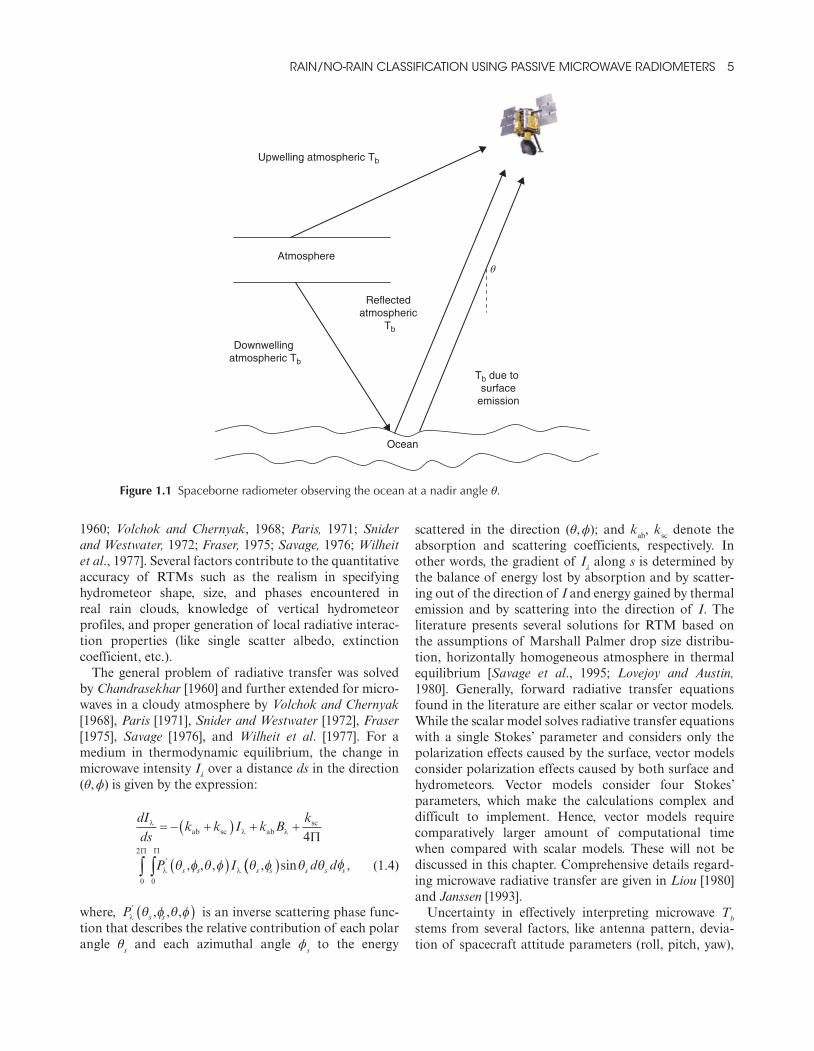
RaiN/No-RaiN ClaSSifiCatioN USiNg PaSSive MiCRoWave RadioMeteRS 5
1960; Volchok and Chernyak, 1968; Paris, 1971; Snider and Westwater, 1972; Fraser, 1975; Savage, 1976; Wilheit et al., 1977]. Several factors contribute to the quantitative accuracy of RTMs such as the realism in specifying hydrometeor shape, size, and phases encountered in real rain clouds, knowledge of vertical hydrometeor profiles, and proper generation of local radiative interac-tion properties (like single scatter albedo, extinction coefficient, etc.).
The general problem of radiative transfer was solved by Chandrasekhar [1960] and further extended for micro-waves in a cloudy atmosphere by Volchok and Chernyak [1968], Paris [1971], Snider and Westwater [1972], Fraser [1975], Savage [1976], and Wilheit et al. [1977]. For a medium in thermodynamic equilibrium, the change in microwave intensity Iλ over a distance ds in the direction (θ, ϕ) is given by the expression:
dI
dsk k I k B
k
P Is s s s
λλ λ
λ λ
= − +( ) + +
( )∫ ∫ ′
ab sc absc
, , , ,
4
0
2
0
ΠΠ Π
θ φ θ φ θ φ(( )sin ,θ θ φs s sd d (1.4)
where, P s sλ′ ( )θ φ θ φ, , , is an inverse scattering phase func-
tion that describes the relative contribution of each polar angle θs and each azimuthal angle ϕs to the energy
scattered in the direction (θ, ϕ); and kab, ksc denote the absorption and scattering coefficients, respectively. In other words, the gradient of Iλ along s is determined by the balance of energy lost by absorption and by scatter-ing out of the direction of I and energy gained by thermal emission and by scattering into the direction of I. The literature presents several solutions for RTM based on the assumptions of Marshall Palmer drop size distribu-tion, horizontally homogeneous atmosphere in thermal equilibrium [Savage et al., 1995; Lovejoy and Austin, 1980]. Generally, forward radiative transfer equations found in the literature are either scalar or vector models. While the scalar model solves radiative transfer equations with a single Stokes’ parameter and considers only the polarization effects caused by the surface, vector models consider polarization effects caused by both surface and hydrometeors. Vector models consider four Stokes’ parameters, which make the calculations complex and difficult to implement. Hence, vector models require comparatively larger amount of computational time when compared with scalar models. These will not be discussed in this chapter. Comprehensive details regard-ing microwave radiative transfer are given in Liou [1980] and Janssen [1993].
Uncertainty in effectively interpreting microwave Tb stems from several factors, like antenna pattern, devia-tion of spacecraft attitude parameters (roll, pitch, yaw),
Atmosphere
Upwelling atmospheric Tb
Downwelling atmospheric Tb
Reflected atmospheric
Tb
Tb due to surface
emission
θ
Ocean
Figure 1.1 Spaceborne radiometer observing the ocean at a nadir angle θ.
0002184420.indd 5 10/13/2014 9:23:45 AM
6 ReMote SeNSiNg of the teRReStRial WateR CyCle
alteration of land surface emissivity during rainfall, nonhomogeneity of land surfaces that results in high and variable surface emissivity, atmospheric attenuation, etc. Attenuation results from the complex interaction of elec-tromagnetic waves with ice, water vapor, oxygen, and other precipitation sized hydrometeors aloft, which can be liquid and/or solid and which may precipitate to surface as rainfall or snowfall depending on the tempera-ture in the subcloud layer. As atmospheric attenuation complicates detection of rainfall signature within Tb, knowledge regarding the sources and sinks of microwave radiation within the atmosphere is crucial to fully under-stand these uncertainties.
1.3. atMosPherIc attenuatIon of MIcrowaves
With the advent of microwave radiometers on board satellites like Defence Meteorological Satellite Program (DMSP), TRMM, Global Precipitation Mission (GPM), Megha Tropiques (MT), etc., microwave rainfall products have become an indispensable source for precipitation infor-mation and for real-time applications in flood forecasting. A choice of frequency channels on board these satellites are made based on the geophysical parameter to be studied and its sensitivity to major atmospheric constituents. Several studies have examined the response of microwave frequency channels due to precipitation-sized particles in the atmos-phere [Weinman and Guetter, 1977; Spencer, 1986; Wu and Weinman, 1984]. Works have also been conducted to esti-mate sensitivity of Tb to variations in atmospheric and pre-cipitation parameters using cloud radiative models such as those by Weinman and Guetter [1977], Wilheit et al. [1982], Wu and Weinman [1984], Szejwach et al. [1986], Olson [1987], and Kummerow and Weinman [1988]. This section describes the field of spectroscopy, an age-old science explained by quantum mechanics during the first half of the twentieth century involving the study of absorption and emission by gases. The five possible ways in which radiation interacts with atmospheric gases are ionization-dissociation interaction, electronic transition, vibrational transition, rotational transi-tion, and forbidden transition [Kidder and Vonder Haar, 1995]. Among these, vibrational and rotational transitions are important for satellite meteorology as they occur mostly in the infrared and microwave portion of the electromagnetic spectrum. Some of the prominent sources causing atmos-pheric attenuation of microwaves are discussed below.
1.3.1. Absorption by Gaseous Atmosphere
An extensive study of microwave absorption of atmos-pheric gases (both theoretically and experimentally) shows that, emission/absorption in gaseous atmosphere is domi-nated by the presence of water vapor and oxygen [Waters,
1976; Ulaby and Stiles, 1981]. Absorption characteristics of these gases are summarized by Staelin [1969], Paris [1971], Derr [1972], Waters [1976], and Fraser [1975]. Microwaves undergo resonant absorption and emission at certain fre-quencies due to the quantum energy states of the water vapor/oxygen molecules. Within microwave spectrum, these molecules are subjected to rotational transition wherein a molecule changes rotational energy states. This causes a peak in Tb measured by a radiometer. The magnitude of increase in Tb depends on the total number of water vapor/oxygen molecules along the propagation path through the atmosphere. At higher altitudes there is a decrease in the number of water vapor/oxygen molecules per unit volume. This in turn reduces the bandwidth of water vapor/oxygen emission (absorption) leading to an increase in absorption at the peak of resonance. The rotational lines of water and oxygen are “pressure broadened” in the atmosphere owing to the presence of other gases; there is also a slight depend-ence on temperature [Kidder and Vonder Haar, 1995]. Water vapor has a weak absorption line at 22.235 GHz and a strong line at 183 GHz. All sensors currently used for pre-cipitation make a measurement near 22.235 GHz like TMI at 21.3 GHz and AMSR at 23.8 GHz. Oxygen has two major peaks, one near 60 GHz and another at 118.75 GHz. More details regarding the absorption characteristics of atmospheric water vapor and oxygen can be obtained from Paris [1971] and Fraser [1975].
1.3.2. Cloud Liquid Water
In an atmosphere with cloud particles, the prominent sources and sinks of microwave energy are local emission and absorption. In the scattering regime, cloud droplets interact weakly with microwave radiation. As the cloud liquid water particles are usually less than 100 µm in diameter, much smaller than the wavelength of radiation, for this Rayleigh region, the scattering effect is negligible. Generally, for the Rayleigh regime, the effect of cloud particles on microwave radiation depends on liquid water content, cloud temperature, and wavelength of radiation. When microwave radiation interacts with rain clouds, the phenomenon is similar to an ensemble of drops with no coherence from drop to drop in the phase of scattered light. Within a rain volume, the usual practice is to assume the raindrops to be randomly distributed. Once we calculate the scattering and absorption for a single drop of spherical dielectric, it is possible by integration to determine corresponding coefficients for a rain cloud that is an ensemble of drops. The particle sizes of raindrops within a rain-bearing cloud are usually described by a continuous function known as drop size distribution (DSD). This function is responsible for defining the con-centration of rain particles per unit volume per unit increment of the drop radius.
0002184420.indd 6 10/13/2014 9:23:45 AM

RaiN/No-RaiN ClaSSifiCatioN USiNg PaSSive MiCRoWave RadioMeteRS 7
Studies by Fraser [1975] estimated the single-scatter albedo as a function of wavelength for DSD representing very thin fair weather cumulus and very dense cumulonim-bus clouds. Generally, for cumulus clouds, scattering remains negligible at all wavelengths. For cumulonimbus clouds raining at 150 mm/h, scattering will be small only for all values of wavelength >~3 cm. Studies by Lovejoy and Austin [1980] concluded that scattering can be neglected for all clouds if wavelength is >0.5 cm, and for rain rate <10 mm/h if wavelength is >1 cm [Stepanenko, 1968; Wilheit et al., 1977]. A complete and published summary of extinc-tion, scattering, and absorption coefficients and scattering phase functions is available in Savage [1978]. Savage approximated the scattering phase functions by Legendre polynomials, and expressed the Legendre coefficients (for the phase function) and extinction, scattering, and absorp-tion coefficients as power law relations in liquid water con-tent [Barrett and Martin, 1981]. Lovejoy and Austin [1980] assessed the relative contribution of cloud droplets and raindrops to total cloud layer absorption and came out with the conclusions that at rain rates = 10 mm/h, cloud absorption was 30–40% as large as rain absorption. This conclusion was consistent with the observations by Gorelik et al. [1971]. In 1976, Savage stated that addition of a non-scattering cloud layer above the rain layer counteracted scattering and resulted in Tb increase by an amount propor-tional to the cloud layer thickness. It must be noted that as cloud droplets, water vapor, and oxygen all absorb (but do not scatter) microwave radiation, they have the potential to confuse precipitation estimates based on absorption [Barrett and Martin, 1981]. Authoritative treatment of this
subject may be found in Gunn and East [1954], Shifrin and Chernyak [1968], Paris [1971], Schwiesow [1972], Hansen and Travis [1974], Savage [1976], and Fraser [1975].
1.3.3. Surface Emission
In the microwave spectrum, an emitting surface must be considered as a gray body so that its emissivity value stays lower than unity. For homogeneous land surfaces, the variability in microwave radiances depends on surface skin temperature and surface emissivity, while the variability for open water bodies is attributed to the atmospheric constituents such as columnar water vapor, temperature profiles, and presence of cloud liquid water. Unlike the oceans, it is very difficult to model land surface properties in the microwave spectrum due to the spatiotemporal variations of soil features like roughness, vegetation cover, and moisture content. The response of different surface types on the temperature and humidity retrievals has been quantified by English [1999]; in these studies microwave emission errors for different continen-tal surfaces were evaluated by using a mathematical tech-nique to potentially extend the low-altitude sounding information over solid surfaces. Microwave land surface emissivity for various surface conditions on a global scale was attempted by Prigent et al. [1998], Weng et al. [2001], and Pellerin et al. [2003].
Different surfaces contribute varying amounts of emis-sion to a microwave radiometer footprint. Figure 1.2 shows the Tb variations for different microwave frequency chan-nels over land and ocean surfaces [Ferraro et al. 1998].
Figure 1.2 Emissivity characteristics of various surface types represented by Tb as a function of frequency (a) over land and (b) over ocean [Ferraro et al., 1998].
300Tb(V) Properties over land
(a)
280
260
240
220
T b(V
) (K
)
200
180
16015 25 35 45 55
Frequency (GHz)
65 75 85
Vegetated land
Heavy rain
Flooded land
Wet snow
Hot desert
Dry snow
Cold desert
Arid land
Light rain
Refrozen snow
(b)Tb(V) Properties over ocean
T b(V
) (K
)
300
280
260
240
220
200
18015 25 35 45 55
Frequency (GHz)
65 75 85
Tropics, clear, calm
Tropics, cloudy, wind
First-year ice
Tropics, clear, wind
Poles, clear, calm
Tropics, convective rain
Tropics, cloudy, calm
Multi-year ice
Midlatitude, stratiform rain
0002184420.indd 7 10/13/2014 9:23:46 AM

8 ReMote SeNSiNg of the teRReStRial WateR CyCle
Oceans provide a stable and uniformly “cold” back-ground for a radiometer, emphasizing more the extinc-tion of upwelling radiation by atmospheric constituents. Emissivity of sea surface is dependent on the dielectric properties of seawater through the Fresnel equation. Studies were conducted to predict the dielectric constant of seawater with an aim to improve the retrieval of atmospheric parameters [Klein and Swift, 1977]. Over snow- covered soil, the emissivity values depend on the dielectric constant of frozen soil (~3), thickness, water equivalent, and liquid water distribution. If snow is dry, Tb decreases with an increase in snow water equivalent. In the case of wet snow, even a small increase in the amount of liquid water causes Tb to rise due to volume scattering. The dependence of snow on Tb is more prominent at microwave frequencies >8–12 GHz. In the presence of vegetation, microwave radiation gets emitted, absorbed, and scattered with the radiative properties mostly con-trolled by the vegetation density, dielectric properties, and relative size of vegetation components with respect to wavelength. Increasing vegetation density increases the emissivity in horizontal polarization and reduces the emissivity polarization difference [Prigent et al., 1997]. In effect, the presence of vegetation reduces the radiometric sensitivity to soil moisture. Studies have developed com-putational schemes to improve the mathematical descrip-tion of surface emissivity for several land types: bare soil, vegetation canopy, and snow-covered terrain [Shi et al., 2002; Ferrazoli et al., 2000; Fung, 1994].
Theoretical models for microwave emission from soils have been presented by many studies [Njoku and Kong, 1977; Wilheit, 1978; Burke et al., 1979; England, 1976] by considering emission from soil for a range of moisture and temperature profiles. At low microwave frequencies, Tb is strongly affected by soil moisture content. This strong dependence is owing to the comparatively high dielectric constant of water (~80) compared to that of dry soil. The dielectric constant of wet soil can reach 20 or more, result-ing in an emissivity change at 1.4 GHz from about 0.95 for dry soil to 0.6 for wet soils. Despite a strong sensitivity of the emissivity on soil moisture, microwave remote sensing of soil moisture from space is complicated due to highly varying surface roughness and vegetation cover, which is aggravated by the presence of mixed surfaces within satel-lite field of view (FOV). To summarize, varying emissivity values from spatiotemporal variations of land surface types can deeply affect radiometer observations, often leading to rainfall retrieval errors.
1.3.4. Ice
Ice particle shapes are crucial in scattering regimes, as they significantly affect the emerging radiance field [Mugnai and Wiscombe, 1986; Bohren, 1986]. Crystals of ice exhibit
a large variety of shapes and modes depending on atmos-pheric temperature and humidity conditions. If we simplify the domain of shapes that the ice nucleation process can create, they can be considered as columns and plates. The usual practice is to adopt a Marshall-Palmer size distribu-tion for ice particle sizes in all theoretical treatments.
Sensitivity of Tb values to the integrated mass of ice/rain depends on frequency, until the optical depth reaches the saturation level [Evans et al., 1995]. Fulton and Heymsfield [1991] studied the response of Tb (18, 37, 92, 183 GHz) to hydrometeors due to intense convection and suggested that even the lowest microwave frequency channel (18 GHz) is significantly obscured by deep convective ice mass. Generally, with an increase in micro-wave frequency (>60 GHz), scattering signatures become more pronounced and a dramatic increase is observed in volume scattering (ks), absorption coefficients (ka), and single-scatter albedo. This is because the aging of ice results in internal voids that tend to scatter microwave radiation. And, an increase in microwave frequencies is accompanied by an increase in the scattering cross section of inhomogeneities, thereby causing a decrease in radia-tion emanating from them. Thus, at higher frequencies, scattering dominates with microwave radiation acting relatively transparently to the rain below freezing level. In satellite meteorology, the high single-scatter albedo pro-duced by ice is crucial, as it heavily depresses high- frequency microwave channels. Ice has much smaller absorption coefficients than water that result in high albedos at all SSM/I frequencies. A single scatter albedo approaching unity indicates that any thermal radiation upwelling from below an ice layer that is attenuated by the ice will be scattered out of the radiometer’s field of view, with very little ice-emitted radiation to replace it [Spencer et al., 1989]. When the scattering coefficient is large, and since there is very little (2.7 K) downwelling radiation from cosmic background, very low values of Tb will be recorded at 85.5 GHz frequency. This extremely low Tb observed is usually attributed to convective rain-fall. Due to the high sensitivity of 85.5 GHz frequency to frozen ice, RNC algorithms for land regions are essen-tially based on ice scattering at this frequency. Studies have also been conducted by Anagnostou and Kummerow [1997] that suggest that as Tb at 85.5 GHz (V) frequency is more variable in raining than in nonraining area, stud-ies of rainfall screening can utilize even the standard deviation of Tb at 85.5 GHz (V) frequency in a 5 × 5 pixel window [Biscaro and Morales, 2007].
1.3.5. Precipitation
At microwave wavelengths, precipitation-sized drops interact strongly with microwave radiation [Kidder and Vonder Haar, 1995]. Interaction of electromagnetic (EM)
0002184420.indd 8 10/13/2014 9:23:46 AM

RaiN/No-RaiN ClaSSifiCatioN USiNg PaSSive MiCRoWave RadioMeteRS 9
waves with a spherical dielectric causes scattering (redirecting) or absorption (conversion to mechanical energy) of radiation depending on the size of precipitation particles [Barrett and Martin, 1981]. One of the earlier studies by Mie [1908] introduced the general mathemati-cal solution for scattering and absorption of EM waves by a dielectric sphere of arbitrary radius. Later on, this was applied to the context of rain by Gunn and East [1954]. The expressions for Mie efficiency factors are given by
Q n
rcexex,λ( ) = σ
Π 2, (1.5)
Q n
rcscsc,λ( ) = σ
Π 2 . (1.6)
In equations (1.5) and (1.6), r denotes the radius of the rain drop, λ stands for the wavelength, and nc represents the complex index of refraction; Qex and Qsc refer to the Mie efficiency factors of extinction coefficient and scat-tering coefficient for a single drop. The symbols σex and σsc represent the effective cross sections for extinction and scattering.
Fraser [1975] has calculated the Mie efficiency factors for extinction and scattering and the Rayleigh extinction coefficient for a range of drop sizes [Barrett and Martin, 1981]. If we consider a single raindrop particle whose size is much smaller than the wavelength of EM waves, Rayleigh approximation to the exact Mie expression applies. The absorption cross section will then be propor-tional to the cube of particle diameter and hence propor-tional to the volume and mass of the raindrop while scattering cross section will be negligible. When cloud drops coalesce into raindrops with dimensions comparable to microwave wavelengths, absorption per unit mass increases and scattering can no longer be ignored. Based on the theoretical calculations by Savage [1976], rain rates of even a few millimeters per hour cause depression (below 260 K) in Tb for microwave frequencies close to 100 GHz. Studies by Kidder and Vonder Haar [1977] used Tb thresh-old values to discriminate raining from nonraining pixels. Although attempts to use measurements at 37 GHz for land regions [Weinman and Guetter, 1977; Spencer et al., 1983; Spencer, 1986] met with partial success, mainly in cases of heavier convective rainfall, more reliable micro-wave rainfall monitoring was made possible only after the launch of SSM/I (1987) [Barrett et al.,1988; Spencer et al., 1989]. Spencer et al. [1989] calculated the scattering and absorption properties of rain for the three main wave-lengths (19.35, 37, 85.5 GHz) that have been used to meas-ure precipitation (Figure 1.3). Their study came out with the conclusions that liquid drops both absorb and scatter microwaves of which absorption dominates [Kidder and Vonder Haar, 1995], especially in the frequency range below 22 GHz. This implies that, in this frequency range,
scattering does not occur and ice particles above rain are nearly transparent. Another prominent result of their study is that with an increasing rain rate, scattering and absorption both increase with microwave frequencies.
1.4. raIn/no-raIn classIfIcatIon Methods
An ideal approach toward understanding the funda-mentals of RNC classification is based on the emissivity characteristics of background surface. RNC algorithms follow different principles when the underlying surface is land or ocean. Ocean surfaces, which appear “cold” to a radiometer operating in the microwave region, offer good contrast for the detection of rain drops, which appear radiometrically warm. As this phenomenon utilizes the strong physical relationship between low-frequency (6–37 GHz) Tb and liquid rainfall, overocean techniques are essentially emission based. Land, however, offers a radiometrically warm background, which tends to hide emission from raindrops. Overland RNC techniques solely rely on ice scattering at a high- frequency (85 GHz) microwave channel and are ambiguous in nature [Wilheit,
280
260
240
220
200
180
160
140
120
100
8010 20 30
Rain rate (mm/h)
85.6 GHz
37 GHz
18 GHz
LandOcean
T b (
K)
40 50 60
Figure 1.3 Relationship of Tb rain rate at 18, 37, and 85.6 GHz. [Reprinted from radiative transfer modeling of Wu and Weinman, 1984.]
0002184420.indd 9 10/13/2014 9:23:47 AM

10 ReMote SeNSiNg of the teRReStRial WateR CyCle
1986; Spencer et al., 1989; Grody, 1991; Adler et al., 1993; Ferraro and Marks, 1995; Lin and Hou, 2008; Wang et al., 2009; Gopalan et al., 2010]. This is mainly due to the highly varying emissivity from the land surface back-ground that clutters rainfall signature. The complicated nature of high-frequency microwave scattering with ice crystals adds to the uncertainty, thereby rendering the use of radiative transfer models extremely difficult. It should be noted that the microwave frequencies are utilized to retrieve several geophysical parameters over ocean; for example, 6.8 and 37 GHz are used for wind speed retrieval [Wentz, 1983], 7 GHz is used for retrieving sea surface temperature [Chelton and Freilich, 2005], and so forth.
Some of the first rainfall screening studies were by Ferraro et al. [1986] and Wentz and Cavalieri [1995]. They proposed using multiple channels to identify a rainfall signature from radiometer-received Tb. Their study, involved an intensive analysis of Scanning Multichannel Microwave Radiometer (SMMR) passes over central North America on 20 January, 1979. The study region was chosen to represent a wide variety of surface and atmospheric features ranging from harsh winter conditions and deep snow cover in the northern latitudes to heavy convective rains.
Based on the criteria of spatial resolution and sensitivity to surface parameters, differences between 18 and 37 GHz channels were selected as the optimum channel combination for rain/no-rain discrimination. Their study observed that the presence of clouds and precipitation led to an increase in Tb. Ferraro et al. [1994] expanded on these ideas and developed a set of geo-graphical screens for land, ocean, semiarid land, coast-lines, and sea ice. Using SSM/I data over ocean surfaces, Wentz and Cavalieri [1995] proposed the no-rain algo-rithm based on the fundamental principles of radiative transfer and explicitly showed the physical relationships between the input (Tb) and the output (wind speed, columnar water vapor, columnar cloud liquid water, rain rate, and effective radiating temperature for upwelling radiation). Later on, this algorithm was extended to include the effects of rainfall. Comprehensive details can be found in Wentz [1997]. The screening methodology that has evolved continuously throughout the years is the Grody-Ferraro screening methodology (discussed in Section 1.4.1). This is currently built in to the GPROF algorithm [Kummerow et al., 2001]. Various versions of GPROF have been applied in SSM/I, TMI, and AMSR-E missions [McCollum and Ferraro, 2003; Wang and Wolff, 2010]. The purpose of this section is to describe the major indices used for demarcating the rainfall signature within a microwave FOV, through which we discuss some of the prominent RNC algorithms adopted for land, ocean, and coastlines, using data from satellites like SSM/I, TRMM, etc.
1.4.1. Scattering Index
The technique of using a scattering index (SI) to deline-ate raining pixels originated from the studies by Grody [1991]. Initially, the idea was proposed to create geo-graphical masks for eliminating Tb cluttering due to desert sand and ice-capped land surfaces. This was essen-tial, as uncertainty in detecting scattering caused by desert/ice-capped surfaces led to false estimates of rain-fall over these regions. RNC algorithms based on SI by Grody [1991] largely relied on regression relationships of microwave low-frequency channels, especially the 19 and 22 GHz. Vertical polarization measurements were pre-ferred, as they resulted in smaller aliasing effects in the presence of mixed boundaries (e.g., coastlines). Adler et al. [1993] devised a global empirical relation for SSM/I to calculate the estimated value of Tb at 85 GHz (V) under nonrainy conditions (Tb Estimated, ), using a fixed quan-tity of 243 K. Later on Ferraro et al. [1994] and Ferraro and Marks [1995] introduced the concept of using low- frequency channel combinations (10–37 GHz) to repre-sent Tb, Estimated. Since the introduction of Grody-Ferraro screening methodology [Ferraro et al., 1986, 1998; Grody, 1991], it has been the most applied technique for use in microwave land precipitation algorithms. The key idea in this technique is that radiation emitted from land sur-faces is affected by ice particles and raindrops at high fre-quency 85 GHz Tb. Calculation of Tb, Estimated involves simulation of 85 GHz Tb values for clear sky conditions (i.e., nonscattering condition). The difference between Tb, Estimated and the observed 85 GHz Tb (Tb, Observed ) gave a measure quantifying the degree of scattering by ice parti-cles and raindrops, wherein the rain rate is proportional to the amount of scattering. As rainfall SI models offered an indirect and nonunique relation that varied from region to region, empirical relationships were largely employed between precipitation and SI to map rainfall over land surfaces [Spencer et al., 1989; Kidd and Barrett, 1990; Conner and Petty, 1998; Adler et al., 1994; Dinku and Anagnostou 2005].
As experience with SI-based studies grew, it became increasingly clear that a new suite of algorithms was nec-essary that efficiently modeled the value of Tb, Estimated to suit the highly varying emissivity from the background land surface. Results of the ensuing development for overland regions are summarized in Table 1.1. Approaches involved using 85 GHz (H) channel instead of 85 GHz (V) channel to depict Tb, Observed [owing to the failure of the first of SSM/I’s 85.5 GHz (V) channel Tb] [Adler et al., 1994; Kummerow and Giglio 1994], using channels of 19 GHz (V) and 22 GHz (V) to represent TB Estimated owing to their increased sensitivity to land surface emissivity. SI-based RNC classification techniques are currently being used for overland RNC classification embedded in
0002184420.indd 10 10/13/2014 9:23:48 AM

RaiN/No-RaiN ClaSSifiCatioN USiNg PaSSive MiCRoWave RadioMeteRS 11
prominent algorithms such as GSCAT and GPROF algo-rithms, which are discussed in Sections 1.4.3 and 1.4.4.
1.4.2. Polarization-Corrected Temperature
Atmospheric hydrometeors have a depolarizing effect on microwave radiation that is emitted and reflected from a highly polarized surface [Wu and Weinman, 1984; Huang and Liou, 1983]. Therefore, polarization offers a great deal of information for separating the highly polarized radiances of the ocean from the essentially unpolarized radiances due to precipitation volume scat-tering [Weinman and Guetter, 1977]. Spencer et al. [1989] proposed an index comprised of linear combinations of vertical and horizontal polarizations to eliminate contrast between land and water/wet surfaces to yield a precipita-tion signal whose interpretation does not vary much depending on the background surface. The conceptual diagram of this index, known as polarization-corrected temperature (PCT) is shown in Figure 1.4.
The PCT relates the vertically and horizontally polarized Tb, and Spencer et al. [1989] described it as a measure of the distance from the no-scattering line. Earlier studies by Spencer [1986] noted that upon addition of nonscattering materials to the atmosphere above a nonraining, oceanic scan spot, the observed Tb will tend to move along the no-scattering line. When scattering materials (e.g., precipitation) gets introduced into the atmosphere, the point moves off the no-scattering line. As scattering lowers the Tb values, observations in which precipitation occurs will essentially fall between the no-scattering line and the no-polarization line. If Tb,HCLF and Tb,VCLF
refer to the horizontally and vertically polar-ized cloud free ocean Tb respectively, Tb,H and Tb,V are the horizontally and vertically polarized Tb that are at least partially affected by any combination of clouds and precipitation, Tb,VOLA and Tb,HOLA are the vertically
and horizontally polarized Tb of the ocean with no over-lying atmosphere, then the expression for PCT is given by
PCT H V=
−
−
β
β
T Tb b, , ,1
(1.7)
Table 1.1 prominent scattering index based Rnc methods
Sl no: Algorithm proposed byObserved Tb (K)
Estimated Tb (K)
SI Threshold (K)
1. Grody [1991] 85(V) 450 2 0 506 1 874 0 00619 22 222. . . ., , ,− × − × + ×T T Tb b bV V V
SI > 10
2. Adler et al. [1994] (GScAT)
85(H) 251 SI > 4
3. Kummerow and Giglio [1994] 85(H) Min[ ],Tb 37 265H, SI > 04. Ferraro [1997] 85(V) 451 9 0 44 1 775 0 00522 22
2. . . ., , ,− × − × + ×T T Tb b b19V V V SI > 10
5. Ferraro [1997] 37(V) 62 18 0 773 19. . ,+ ×Tb V SI > 56. Kummerow et al. [2001]
(GpROF)85(V) Tb, 22V SI > 8
7. M1 [Seto et al., 2005] 85(V) μ SI > k0σ8. M2 [Seto et al., 2005] 85(V) a b Tb+ × ,22V SI > k0σe
Source: Modified and adapted from Seto et al. [2005].
Precipitation
Constant β(slope)
Cloud-freeocean
Atmosphere-freeocean
Tb(H)
“Background”PCT
Storm PCT
Tb(V)≈ 288 K
@ 85 GHz
≈ 288 K@ 85 GHz
T b(V) =T b(H
)
Figure 1.4 Schematic diagram of vertically and horizontally polarized Tb of ocean with and without an overlying atmos-phere [Spencer et al., 1989].
0002184420.indd 11 10/13/2014 9:23:51 AM
12 ReMote SeNSiNg of the teRReStRial WateR CyCle
where
β =
−
−
T T
T Tb b
b b
, ,
, ,
.VCLF VOLA
HCLF HOLA
(1.8)
Calculation of PCT at any frequency requires a nearly constant value of β. Experiments using SSM/I observa-tions of global cloud-free oceanic areas show that to obtain a physically meaningful value of PCT (between 275 and 290 K) the value of β should be 0.45. Absolute accuracy for β is not as important as keeping it constant in all subsequent calculations. Equation 1.7 for PCT can be rewritten as
PCT T Tb v b h= −1 818 0 818. ., ,
(1.9)
PCT values using 85.5 GHz frequency channels will generally be lower than the background PCT, although its Tb depression will be much less than that due to the strong volume scattering effects of precipitation. Hence, this property of 85.5 GHz PCT is employed to detect cloud liquid water. Studies by Mugnai et al. [1993] using numerical model simulations demonstrated that 85 GHz signals represent emissions from upper-level liq-uid and ice scattering in the upper reaches of tall pre-cipitation clouds. Therefore, PCT using 85.5 GHz channel is sensitive to precipitation top height for tall convection and surface rainfall for moderate convec-tion. A modified relation for PCT was proposed by Kidd and Barret [1990] using SSM/I’s 85.5 GHz chan-nels as the basis for estimation of precipitation over both land and water. PCT is currently being used for RNC classification and the succeeding rainfall retrieval oceans and coastlines in the algorithm of the GSMaP, which is discussed in Section 1.4.4
1.4.3. Goddard Scattering Algorithm
The Goddard scattering algorithm (GSCAT) was first proposed by Adler et al. [1993]. Their study detected the existence of rainfall signature using an empirical logic tree applied to multiple channels. The algorithm relied on frequencies of 86 and 37 GHz (both in the horizontal polarization) to eliminate nonraining areas. This tech-nique worked well over ocean and land areas but suffered from the inability to detect rain from clouds below the freezing level. Efforts were undertaken to modify the GSCAT RNC algorithm by including geographical screens (for deserts and snow-covered surfaces) similar to the work by Grody [1991]. Adler et al. [1994] modified this algorithm and included better quality control and use of lower frequency channels to differentiate cold surface and desert from precipitation. This differentiation was
essential when rainfall retrieval is to be made globally. Adler et al. [1994] and Kummerow and Giglio [1994] created GSCAT2, which used 85 GHz (H) instead of 85 GHz (V), to represent the value of Tb,Observed and a constant value (251 K) for Tb, Estimated without using any regression equations such as Grody [1991]. It was devel-oped using channel information from SSM/I sensors. The methodology employed several checks, including the existence of cold ocean, coastline, desert, ice-covered regions, and ambiguous cold surface possible precipita-tion checks. These checks prevented surface effects that might lead to false identification of rain regions. GSCAT-2 proved to perform successfully in the SSM/I era to demarcate rain/no-rain regions, but not without some false rain identifications. The overall procedure for identifying raining pixels was not all that dissimilar from the scattering index by Grody [1991]. In an intercompari-son study involving seven microwave techniques over Japan, Lee et al. [1991] showed that the GSCAT had the highest correlation with the Grody scheme during the convective regime in July–August 1989. The scattering signatures in GSCAT were used to retrieve rain intensity in proportion to the amount of scattering by ice and graupel aloft based on radiative transfer calculations applied to numerical cloud model results.
1.4.4. Goddard Profiling Algorithm
The GPROF algorithm is considered the established algorithm framework for microwave rainfall products from TRMM (launched in November 1997), Aqua (satel-lite of AMSR-E launched in May 2002), and included in the initial plans for the proposed Global Precipitation Measurement (GPM) mission (to be launched in 2014). GPROF follows separate sets of algorithms for RNC classification over land, ocean, and coastlines. Various versions of GPROF screening methodology have been implemented in SSM/I, TMI, and AMSR-E missions with an improved version to be applied in GPM mission [McCollum and Ferraro, 2003; Wang et al., 2009; Gopalan et al., 2010].
1.4.4.1. RNC Over LandThe RNC classification algorithm of GPROF for land
regions [Kummerow et al., 2001] assumes that Tb at 21.3 GHz (V) represents the nonscattering portion of Tb from 85 GHz (V). A scattering index threshold of 8 K is fixed to judge rainfall signature from a pixel/footprint. All pixels that exceed this threshold were identified as “possible rain” and were then processed using the full Bayesian algorithm to quantify the rain rate, which could be zero or nonzero. GPROF version 4 used the screening methodol-ogy of GSCAT 2 [Adler et al., 1994]. Version 5 of GPROF [Petty 1994] employed polarization-based emission and
0002184420.indd 12 10/13/2014 9:23:52 AM

RaiN/No-RaiN ClaSSifiCatioN USiNg PaSSive MiCRoWave RadioMeteRS 13
scattering indices that could isolate signal coming from rain clouds with the background variability.
1.4.4.2. RNC Over OceansOver oceans, the predictable ocean surface emissivity
offers contrast to the signals emanating from liquid hydrometeors over the range of microwave frequencies. Yet, the RNC detection technique of TRMM TMI usually fails over oceans to detect shallow rain observed by PR owing to the small scale of shallow rain when compared with the resolution of channels used in the emission-based algorithm. As clouds are optically thick at 85 GHz, it becomes very difficult to use the emission-based algorithm to detect shallow rains. Owing to the contrast between atmospheric liquid and low emissivity ocean surface, screening rainfall pixels over oceans relies on estimation of the liquid water path (LWP). The screen-ing of GPROF over the ocean consists of two processes: checking the LWP and screening out clear ocean pixels and ice surface pixels. The flowchart for GPROF method over the ocean is shown in Figure 1.5.
In the first process, based on the study of Karstens et al. [1994], the LWP is checked using TMI low-resolution chan-nels of 22 GHz (V) and 37 GHz (V) using the relation
LWP = −( ) − −( )+0 39 285 1 40 285
4 2922 37. log . log
. ., ,T Tb V b V
(1.9)
All the footprints having LWP values less than the maxi-mum LWP was classified under “no rain,” where the value of maximum LWP (kg /m2) is based on the follow-ing relation:
LWP
FLH_max . * .=
0 25
4000 (1.10)
Here the value of freezing level height (FLH) is derived from the work by Wilheit et al. [1991] and the values of 0.25 and 4000 represent the liquid water content and a typical FLH [Wilheit et al., 1991].
The second process was based on the GSCAT algo-rithm [Adler et al., 1994], which employed three checks. The first check employed threshold values for Tb from 22 GHz (V) and 85 GHz (H) channels to identify the target pixel as “possibly rain.” This check was origi-nally used to screen ice surfaces and “possible rain,” but in the GPROF version 6 algorithm, this was utilized to detect rainfall signature. The second check aimed to distinguish ice surfaces from “rain” using Tb at 22 GHz (V). The third check was to identify clear ocean using Tb at 37 GHz (H) and 85 GHz (H). If the target pixel was not identified as ice surface/clear ocean by these checks, it was flagged as “possible rain.” After the screening process, the footprints identified as “possible rain” are processed using the Bayesian algorithm to quantify rain rate.
Is LWP < LWP_max No rain(clear ocean)
Is Tb,85H> 262.0Is Tb,22V< 269.1
Is Tb,22V< 192.0
Is Tb,85H– Tb,37V> 0.5Is Tb,37V≤ 186.7
Rain possible
No rain(ice surface)
No rain(clear ocean)
Rain possible
Apply Bayesian algorithm
No rain RainR = 0 R > 0
Checking of LWP
Checkingfor clearocean &
ice surface
Figure 1.5 Flowchart for Rnc method of GpROF over ocean [Kida et al., 2009].
0002184420.indd 13 10/13/2014 9:23:52 AM

14 ReMote SeNSiNg of the teRReStRial WateR CyCle
Tb,85H > 257, Tb,22V < 269.1
Tb,22V <192
Tb,85H − Tb,37H > 0.5Tb,37H < 186.7 > 257
Tb,37H − Tb,85H > 10.5 Tb,22V > 37.9 + 0.88 × Tb,19V Tb,22V < 269.1
Tb,22V < 269.1Tb,22V > 37.9 + 0.88 × Tb,19V
Tb,22V < 261.9Tb,22V < 163.3 + 0.49 × Tb,85H
Tb,22V < 261.9Tb,22V < 0.49 × Tb,85H + 163.3
No
No
Ambiguous
Yes
Yes
No
Tb,22V < 269.1
No
Possible rain
No
AmbiguousNo rain (ice)Yes
No
Tb,22V < 269.1Yes
NoNo
YesPossible rain
Yes
No
YesYes
Clear coast check
No
YesPossible rain
YesNo rain (ice)
No rain (open ocean)Yes
No
Ambiguous
YesNo rain Ambiguous No
Figure 1.6 Decision tree for demarcating rainfall over coasts (HA93) [McCollum and Ferraro, 2005].
1.4.4.3. RNC Over CoastsRain identification over land or water involves checks
for snow/desert surfaces, which tend to depress the high-frequency microwave channels. Coastlines are much more difficult as, for either water or land surfaces, adding the opposite surface into the footprint will have the same effect as rainfall. Over land, adding surface water to the footprint will reduce the Tb’s, as does scat-tering caused by rain, and adding land to a water foot-print will increase Tb’s, similarly to rain over water, resulting in emission [McCollum and Ferraro, 2005]. Over coasts, microwave footprint is a combination of radiometrically warm land surface and cold ocean sur-face. One of the very first RNC algorithms developed for coasts was using SSM/I channels by Adler et al. [1994]. They proposed a complex decision tree method as shown in Figure 1.6, to isolate rainfall signature without using the SI method by Grody [1991]. More details about this method are available in Huffman and Adler [1993], which will hereinafter be referred to as HA93. The HA93 algorithm was implemented in GPROF and has remained in use in successive GPROF versions [Wilheit et al., 2003].
Bennartz [1999] provided a technique to account for the coastline complexity, which involved use of effective antenna pattern function and scan geometry of the microwave instrument and high-resolution land-water mask to analyze the fraction of land versus water within each radiometer footprint. The study represented the atmospheric contribution from rain assuming a constant land Tb, while the land versus water fraction was used to weight the relative contri-bution of land-ocean surfaces to background signal. This technique was implemented to retrieve column water vapor for noncloud conditions using SSM/I data for the Baltic Sea region of western Europe. The study concluded that satellite navigation uncertainty created a dominant source of error. The assumption of a constant value to represent Tb from highly vary-ing land surfaces fails in raining situations, for which cases the method of Bennartz [1999] cannot be imple-mented. The land surface emissivities have not yet been incorporated in the land component of GPROF rainfall algorithms. And, use of a straight cutoff for Tb values also cannot be implemented over coasts as water within the footprint reduces the high-frequency
0002184420.indd 14 10/13/2014 9:23:53 AM

RaiN/No-RaiN ClaSSifiCatioN USiNg PaSSive MiCRoWave RadioMeteRS 15
Tb’s. As a result, combination of several criteria were examined to classify a footprint as having “no rain,” “possibly rain,” or “ambiguous.” The criteria were mostly determined from the studies of Grody [1991] and Adler et al. [1993].
The HA93 decision tree method for RNC classifica-tion of coastline is summarized in figure 1.6. In this figure, the “clear coast check” by Adler et al. [1993] involves the following checks for Tb from 85 GHz (H) and 37 GHz (H):
σ T Kb, ,85 10H( ) > (1.11)
ρ T Tb b, , . ,37 85 0 5H H,( ) > (1.12)
Slope <1 2. , (1.13)
where
Slope ,H H
H
H
= ( ) ( )( )
ρσ
σT T
T
Tb b
b
b
, ,
,
,
,37 85
85
37
and σ (standard deviation) and ρ (cross correlation) are computed on a 5 × 5 footprint array centered on the footprint of interest. This test identifies cases in which low humidity allows the (similar) surface emission signals from Tb,37H and T Tb b, ,/85 89H H to dominate the microwave signal [McCollum and Ferraro, 2005].
The HA93 algorithm added ambiguous classes for TB combinations for which rainfall rate was retrieved based on the requirement that another scheme be applied to estimate whether the retrieval was useful or an artifact. In case this could not be done, no estimate was made for such foot-prints in the “ambiguous” class, leaving “holes” in the resulting rainfall map. Footprints that were classified under “possible rain” were required to satisfy a cutoff threshold using higher frequency channels to be flagged as “rain” over land regions. The HA93 algorithm used Tb,85 257H K< criterion to assign a positive rain classification. The study conducted by McCollum and Ferraro [2005] using AMSR-E data suggested that a threshold using Tb,85H fails to provide a clear cutoff. The availability of TMI Tb’s collocated with TRMM PR rainfall rates enabled choosing cutoff criteria that could efficiently separate raining from nonraining footprints. To summarize, the study by McCollum and Ferraro [2005] provided two major improvements to the existing RNC classification algorithm for coasts. The first step was to estimate conditions where positive rain rates should be estimated rather than leaving the areas without estimates as in the previous algorithm. Owing to the high correlation among the various TMI microwave channels, principal component analysis often provides a useful
technique to separate signals of geophysical variables by the creation of mutually orthogonal statistically uncorre-lated eigenvectors [Conner and Petty, 1998]. Therefore, the second step modified the cut-off threshold for rain/no-rain classification by using a PCT criterion instead of a straight Tb cut-off. These modifications were implemented in 2004 for the version 6 TMI product and third release of AMSR-E products with a slight difference for each product. The significant changes implemented for the latest version (ver-sion 7) of the GPROF TMI ocean algorithm involves addi-tion of the probability of precipitation parameter, wherein pixels are not screened before Bayesian scheme. The algo-rithm developers recommend using 50% probability of rainfall threshold within the FOV when comparing with instantaneous PR and TMI rain rates. For the TMI coastal algorithm, a change in the land/ocean classification has been implemented [Zagrodnik and Jiang, 2013].
1.4.5. Global Satellite Mapping of Precipitation (GSMaP) Algorithm
The GSMap algorithm was developed by the Earth Observation Research Center, Japan Aerospace Exploration Agency (JAXA/EORC), and has been further improved with the use of PR measurements. Comparative studies by Kummerow et al. [2001] evalu-ated the performance of TRMM monthly rainfall esti-mates from both its sensors TMI and PR, which revealed a bias between both the rainfall products of nearly 30% over ocean and 26% over land (using version 5 of data products). The TRMM version 6 algorithms display improvements within level 2 surface rain retrieval algo-rithms based on physical principles. Results of inter-comparison studies between version 5 and version 6 algorithms are presented in Chiu et al. [2006]. GSMaP is drawn up to the highest levels of precision and resolu-tion with temporal resolution of 1 h and spatial resolu-tion of 0.1°. The RNC algorithms implemented in GSMaP for over land, over ocean, and coastal regions are discussed below.
1.4.5.1. RNC Over Land
Seto et al. [2005] developed the RNC classification algo-rithm (version 4.5) for GSMaP that was employed in TRMM. Their study involved statistically summarizing all the TMI Tb values under no-rainfall conditions of PR 2A25, for the land regions into a database that represented both the spatial and temporal variations of Tb. This “land surface brightness temperature database” contained the spatiotem-poral variations of Tb including the effects of sand and fallen snow [Seto et al., 2005]. Due to the varied spatial reso-lutions of TMI channels among themselves as well as with PR, footprint size was defined by means of effective field of view (EFOV). PR footprints, the center of which lie within a
0002184420.indd 15 10/13/2014 9:23:54 AM

16 ReMote SeNSiNg of the teRReStRial WateR CyCle
TMI footprint, were chosen as reference. In their study, all the PR observations within a TMI footprint that had a “no-rain” or “rain-possible” flag were adjudged to be in no-rain conditions. Their study summarized TMI observations under no-rain conditions in a database with resolution of 1 month and 1° latitude × 1° longitude. The distribution of Tb values under no-rain conditions was represented using a Gaussian distribution. The mean (μ) and standard deviation (σ) of 85 GHz (V) Tb were calculated to represent the distri-bution and stored in the database.
Seto et al. [2005] proposed two RNC methods (named as M1 and M2) for real-time use. The first method (M1) used the parameters estimated from the database of TMI Tb under no-rain conditions. The value for Tb, Estimated was fixed as equivalent to μ and the threshold of scattering was judged at k0σ where k0 was a constant in space and time. The thresholds for M1 differed with month and grid. This was an improvement over the threshold of Adler et al. [1994], which remained fixed at a constant value of 251 K. M2 considered a linear regression fit using least mean square error, between Tb (21.3 V) and Tb (85.5 V), both under no-rain conditions, using the database.
T a b Tb b, ,. .~85 5 21 3V NoRain V NoRain( ) + ( ) (1.14)
The subscript denotes observations conducted under no-rain / clear sky conditions. If σe is the standard deviation of
residuals of equation and k0 is a constant in both space and time, the pixel fulfilling the criterion of equation (1.11) is adjudged as containing a rainfall signature:
T T kb b e, ,. .85 5 85 5 0V Estimated V Observed( ) − ( ) > σ (1.15)
The number of rain pixels increased or decreased depend-ing on the value of k0, which varied with regions and sea-sons. The usual practice was to affix a constant value for k0 for simplicity reasons. For GSMaP, the value of k0 adopted was 3.5 and no desert/snow masks were employed as in Grody [1991]. The proposed RNC for version 4.7 was the same as that of version 4.5 with the only difference being in the retrieval part. These RNC methods are also known as PR-dependent methods as they cannot be applied to other microwave radiometers not accompanied by spaceborne precipitation radar. The methods (M1 and M2) were modi-fied with an aim to make the RNC methods independent of PR so that these could be applied to data from other micro-wave radiometers as well. Comprehensive details regarding these can be found in Seto et al. [2009].
1.4.5.2. RNC Over OceansOver oceans, GSMaP adopted the method of Kida
et al. [2009]. Their study employed two stages for detection of rain and no-rain footprints, as shown in Figure 1.7. In the first stage, deep rain pixels were
Rain85 > 1
Within the range of 10 GHzEFOV from a target pixel
PCT37V< 1
Tb,10V_Ra inf ree< Tb,10V
And/or
Tb,19V_Ra inf ree< Tb,19V
Tb,10V_Ra inf ree< Tb,10V
And/or
Tb,19V_Ra inf ree< Tb,19V
And/or
Tb,37V_Ra inf ree< Tb,37V
Rain
No rain
No rain
No
Yes Yes
No
No
First stage
Second stage
Figure 1.7 Flowchart for Rnc classification used in GSMap [Kida et al., 2009].
0002184420.indd 16 10/13/2014 9:23:55 AM

RaiN/No-RaiN ClaSSifiCatioN USiNg PaSSive MiCRoWave RadioMeteRS 17
determined by Tb from 85 GHz (V) scattering signature, and shallow rain pixels were determined with normal-ized polarization difference at 37 GHz (V). The study considered all the pixels of 85 GHz (V) lying within the EFOV of 10 GHz (V) pixel. The condition for detec-tion of deep rain pixel was then fixed as the existence of one or more pixels of 85 GHz (V) within the EFOV of 10 GHz (V), having a rain rate > 1mm/h (rain 85 pixels). The study classified the target pixel (central pixel) as deep rain pixel upon fulfilling the above con-dition. If not, the normalized PCT [Petty, 1994] as given by equation 1.12 was used to check the existence of shallow rain:
PCT V H
V H37
37 37
37 37V
b b
b b
T T
T T=
−
−, ,
, _ inf , _ inf
.Ra ree Ra ree
(1.16)
Based on the results of the first stage, their study checked emission signatures from raindrops in the second stage. The three checks used in the second stage are shown in Figure 1.7 from which it can be seen that Tb values of channels 19 GHz (V), 10 GHz (V), and 37 GHz (V) were used.
Kida et al. [2009] proposed modifications for the RNC method of GSMaP in order to use Tb from 37 GHz (V) more efficiently. Their study was essentially a PR-dependent method wherein the level 2 standard product 2A25 [Iguchi, 2007] was used as the validation product. Their study modified two conditions used in the first stage of GSMaP. In the original GSMaP algorithm,
for the first stage, in the presence of pixels whose rain 85 > 1 mm/h within the EFOV of 10 GHz (V), the cen-tral target pixel was identified as a deep rain pixel, even if it may actually be a shallow rain pixel. This led to misclassification of most of the shallow rain pixels as no-rain pixels (Figure 1.8). Kida et al. [2009] modified the first-stage algorithm by checking the rain rate of 85 GHz (V) Tb pixel just for the target pixel, to avoid mis-classification of shallow rain pixels as deep rain pixels. The second modification was use of 37 GHz (V) Tb instead of normalized PCT to detect shallow rain. This was because Tb at 37 GHz (H) was known to be more sensitive to wind speed than Tb at 37 GHz (V). With increase in wind speed, Tb at 37 GHz (H) increases more than Tb at 37 GHz (V). And in the case of an extraordi-nary event such as a typhoon, characterized by strong wind speed, PCT (using 37 GHz) will be less than 1, leading to misclassification of shallow rain in windy regions. Hence, their study preferred Tb from 37 GHz (V) channel, which was less sensitive to wind speed variations.
1.4.5.3. RNC Over CoastsOver coastal areas, GSMaP used the RNC algorithm
proposed by Kubota et al. [2007]. Their study was an improvement over the RNC detection method of McCollum and Ferraro [2005], which detected precipitat-ing areas using PCT index at 85 GHz (V) and a decision tree of several empirical conditions for TMI Tb’s. Kubota et al. [2007] used the condition of surface temperature < 273.2 K for flagging no-rain pixels over coastal areas.
Deep rain pixelsof 85 GHz
Shallow rainpixel
Target pixel of 85 GHzmisclassified as a deeprain pixel
EFOV of 10GHz
Figure 1.8 Example of a shallow rain pixel being misclassified as a deep rain pixel [Kida et al., 2009].
0002184420.indd 17 10/13/2014 9:23:55 AM
18 ReMote SeNSiNg of the teRReStRial WateR CyCle
The previously employed condition of Tb,85H > 257, Tb,22V < 269.1 leads to false rainfalls during the winter in mid-latitude coastal areas and hence is avoided. Kubota et al. [2007] classified ambiguous class into “possible rain” and “no-rain” classes. Instead of using a PCT cutoff thresh-old, their study applied a scattering index threshold of RainPCT85 > 1, to possible rain cases. Here, rainPCT85 stands for rain rate from PCT index calculated using 85 GHz (V) channel frequency. Selection of a suitable thresh-old for RNC classification is as important as deriving the algorithm itself. For the GMSaP algorithm, Kida et al. [2008] proposed a parameterization of rain/no-rain threshold value of cloud liquid water as a function of storm height based on CloudSat precipitation product and the cloud liquid water derived from Aqua/AMSRE.
1.5. rnc PerforMance analysIs
RNC classification is a typical example for dichoto-mous classification having just two probabilities of either zero (denoting “no”) or unity (denoting “yes”) whose result can be expressed in 2 × 2 contingency matrix as shown in Table 1.2. In Table 1.2, the element a denotes the number of correct (or yes) forecasts of an observed event, c refers to the number of events that occurred but were not forecast, b is the number of forecasts of events that did not occur, and d is the number of correct fore-casts of events that did not occur. It should be noted that Table 1.2 depicts dichotomous classification wherein col-located TMI and PR observations are analyzed assuming PR observations to be “true” or near perfect. Some stud-ies increase the resolution of low-frequency channels by linear interpolation to match the resolution of 85 GHz (V) channels. Data collocation can then be performed using the geolocation information from TRMM PR and TMI data set to assign a TMI pixel at the 85 GHz (V) resolution as the nearest neighbor for every PR pixel in an orbit [Gopalan et al., 2010; Indu and Kumar, 2013]. Data collocation has also been carried out by aggregating all of the PR observations within a TMI footprint before skill score calculations [Seto et al., 2005]. This section
discusses some of the statistical descriptors used to ana-lyze performance of this binary classification. The com-monly used indices for RNC accuracy assessment are summarized in Table 1.3.
The most commonly used indices are the probability of detection (POD) or prefigurance [Panofsky et al., 1965] and the false alarm ratio (FAR). POD is the likelihood that an event would be estimated, given that it occurred, whereas FAR is an element of the conditional distribution of events given the estimate. Due to the negative orientation of FAR, smaller values indicate better esti-mates [Wilks, 1995]. Another measure used to compare the average estimate with the average observations is the frequency bias (B). B signifies the ratio of number of yes estimates to the number of yes observations. In this meas-ure less than one indicates underestimation and greater than one indicates overestimation. The threat score (TS) or critical success index (CSI) indicates the number of cor-rect yes estimates divided by the total number of occa-sions on which the event was estimated or observed [Wilks, 1995]. CSI has been widely used as a performance meas-ure for rare events (as rainfall extremes) as it does not use the content of null events, as in POD and FAR [Montero-Martinez et al., 2012]. These indices help to answer ques-tions regarding meteorological aspects such as: (1) How reliable is a product in detecting precipitation? (obtained using POD); (2) How to quantify overall bias of satellite estimates using ground truth? (obtained using B); (3) How often does a product indicate precipitation during nonpre-cipitating scenarios? (obtained using FAR).
Performance analysis of binary classification can also be characterized using relative accuracy measures or skill scores. Skill scores quantify the agreement between fore-cast and observations [Tartaglione, 2010]. A skill score is the ratio of differences [Stanski et al., 1989; Wilks, 1995] of scalar representations of the classification perfor-mance. An estimating scheme cannot be useful if it yields skill scores that can be obtained by less sophisticated esti-mating procedures [Storch and Zwiers, 1999]. It is to be noted that no single skill score can be used to indicate forecast skill. Hence, various skill scores or relative accu-racy measures are derived from the contingency table. Different skill scores perform differently. Some of the skill scores used are Heidke skill score (HSS), Kuiper skill score (KSS), Gilbert skill score (GSS), and odd’s ratio skill score (ORSS). The reference accuracy measure in the HSS [Heidke, 1926] is the hit rate of random estimates, subject to the constraint that the marginal distributions of estimates and observations characterizing the contingency table for the random estimates are the same as the mar-ginal distributions in the actual verification data set [Wilks, 1995]. HSS is a generalized skill score that tends to elimi-nate classifications occurring purely due to chance. Thus, perfect classification yields HSS value of 1, which implies
Table 1.2 Layout of contingency matrix a
Event Observed
Rain Judged by pR (Yes)
no Rain Judged by pR (no)
Event ForecastRain judged by TMI
(Yes)a b
no rain judged by TMI (no)
c d
a Assuming that the rainflag by pR is near perfect and can be used as validation data.
0002184420.indd 18 10/13/2014 9:23:56 AM
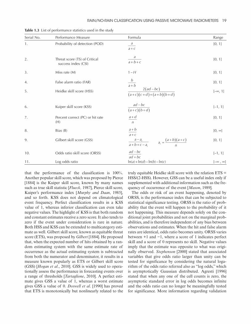
RaiN/No-RaiN ClaSSifiCatioN USiNg PaSSive MiCRoWave RadioMeteRS 19
that the performance of the classification is 100%. Another popular skill score, which was proposed by Pierce [1884] is the Kuiper skill score, known by many names such as true skill statistic [Flueck, 1987], Pierce skill score, Kuiper’s performance index [Murphy and Daan, 1985], and so forth. KSS does not depend on climatological event frequency. Perfect classification results in a KSS value of 1, whereas inferior classification can even take negative values. The highlight of KSS is that both random and constant estimates receive a zero score. It also tends to zero if the event under consideration is rare in nature. Both HSS and KSS can be extended to multicategory esti-mate as well. Gilbert skill score, known as equitable threat score (ETS), was proposed by Gilbert [1884]. He proposed that, when the expected number of hits obtained by a ran-dom estimating system with the same estimate rate of occurrence as the actual estimating system is subtracted from both the numerator and denominator, it results in a measure known popularly as ETS or Gilbert skill score (GSS) [Hogan et al., 2010]. GSS is widely used to opera-tionally assess the performance in forecasting events over a range of thresholds [Tartaglione, 2010]. A perfect esti-mate gives GSS a value of 1, whereas a worst estimate gives GSS a value of 0. Doswell et al. [1990] has proved that ETS is monotonically but nonlinearly related to the
truly equitable Heidke skill score with the relation ETS = HSS/(2-HSS). However, GSS can be a useful index only if supplemented with additional information such as the fre-quency of occurrence of the event [Mason, 1989].
The odds or risk of an event happening, denoted by ORSS, is the performance index that can be subjected to statistical significance testing. ORSS is the ratio of prob-ability that the event will happen to the probability of it not happening. This measure depends solely on the con-ditional joint probabilities and not on the marginal prob-abilities, and is therefore independent of any bias between observations and estimates. When the hit and false alarm rates are identical, odds ratio becomes unity. ORSS varies between +1 and −1, where a score of 1 indicates perfect skill and a score of 0 represents no skill. Negative values imply that the estimate was opposite to what was origi-nally observed. Stephenson [2000] stated that associated variables that give odds ratio larger than unity can be tested for significance by considering the natural loga-rithm of the odds ratio referred also as “log odds,” which is asymptotically Gaussian distributed. Agresti [1996] stated that when any one of the cell counts is zero, the asymptotic standard error in log odds becomes infinite and the odds ratio can no longer be meaningfully tested for significance. More information regarding validation
Table 1.3 List of performance statistics used in the study
Serial no. performance Measure Formula Range
1. probability of detection (pOD) aa c+
[0, 1]
2. Threat score (TS) of critical success index (cSI)
aa b c+ +
[0, 1]
3. Miss rate (M) 1 − H [0, 1]
4. False alarm ratio (FAR) ba b+
[0, 1]
5. Heidke skill score (HSS) 2 ad bc
a c c d a b b d
−( )+( ) +( ) + +( ) +( )
[–∞, 1]
6. Kuiper skill score (KSS) ad bca c b d
−+( ) +( )
[–1, 1]
7. percent correct (pc) or hit rate (H)
a dn+ [0, 1]
8. Bias (B) a ba c++
[0, ∞]
9. Gilbert skill score (GSS) a aa b c a
r
r
−+ + −
aa b a c
nr =+( ) +( ) [0, 1]
10. Odds ratio skill score (ORSS) ad bcad bc
−+
[–1, 1]
11. Log odds ratio ln(a) + ln(d) − ln(b) − ln(c) [–∞ , ∞]
0002184420.indd 19 10/13/2014 9:23:57 AM
20 ReMote SeNSiNg of the teRReStRial WateR CyCle
of satellite-based precipitation estimation can be obtained from the research by the International Precipitation Working Group (IPWG) (http://www.isac.cnr.it/~ipwg/IPWG.html ).
It should be noted that the performance of an RNC algorithm is strongly affected by the spatial and temporal scales for rainfall detection and the rainfall detection threshold. Identification of an optimum threshold for RNC classification depends on the missed rain amount, false rain amount, and most importantly on the user requirements. If the end product is to generate rain maps for flood warning, a lower threshold should be fixed for safety reasons. A larger threshold value is preferred if the resulting rain map is to be used for drought warning [Seto et al., 2005]. Difference in spatial resolutions of multifre-quency satellite microwave observations is a common problem in RNC classification and subsequent rainfall retrieval process. Usage of channels with larger FOV will incorporate more noise from outside the test area, thereby resulting in decreased accuracy. When the radiometer FOV is partially filled with cloud or rain, it results in beam filling effects that have been well documented in many studies [Melitta and Katsaros, 1995; Greenwald et al., 1997; Bremen et al., 2002; Chiu et al., 1990; Short and North, 1990; Kummerow et al., 1998]. Some studies have used techniques to deconvolve the TMI Tb’s at 10 GHz and convolve at 21–85 GHz to a common FOV cor-responding to 19 GHz (H) FOV [Backus and Gilbert, 1970]. A resampling technique is applied to the TMI data to perform this operation using a linear combination of nearby observations using knowledge regarding TMI antenna patterns and scan geometry. The crucial points to be considered are the parallax effects between the instruments (e.g., TMI and PR) and their antenna pat-tern, the inclusion of signals from outside the EFOV if footprint is defined using EFOV, beam filling effects, and the like [Bauer et al., 2002]. Studies showing temporal variations of FAR and POD for various RNC algorithms were presented in Seto et al. [2005]. Their study revealed that diurnal variations in the physical temperature of land surface cause Tb values of no-rain pixels to be lower at night. This directly implies that at night, a constant rainfall detection threshold for Tb will tend to produce a higher FAR.
1.6. oPen QuestIons
The ultimate goal of RNC classification is to produce the most accurate detection of rainfall signature from microwave footprints over any background surface (land, ocean, coast). Since the accuracy of RNC algorithms is tied to the characteristic properties of microwave data in multiple frequency channels, the need to understand and improve quality of information retrieved from various
channels is obvious. There remain several open questions that need to be addressed such as uncertainty due to RNC, inability of present algorithms to detect light rain, and so forth. Here, we outline some important questions and possible future research directions.
1.6.1. Resampling/Matchup Errors
The distribution of microphysical parameters, precipi-tation cells, cloud cover, and associated volume absorp-tion and scattering coefficients are subjected to large variability within a microwave radiometer footprint [Smith and Kidder, 1978; Austin and Geotis, 1978; Mugnai and Smith, 1988]. For quantitative assessment of rain/no-rain classification, by far the biggest issue is the nonuniform spatial resolution wherein diffraction limits the attainable resolution. Microwave footprints are characterized with large horizontal resolution (FOV). And when information from multiple frequencies having differing resolutions need to be combined to retrieve geophysical parameters, which are not necessarily homogeneous over the footprint area, the problem of resolution mismatch becomes criti-cal. The literature presents several approaches to solve this issue in the form of simple averaging of high-resolution measurements to match the low-resolution data, matching the resolution of all the frequencies to a common 25 km spatial resolution. Backus and Gilbert [1970] proposed a technique for inverting seismic data in order to retrieve Earth density profiles. This technique reconstructed meas-urements at different resolutions from those originally sampled using a combination of oversampled measure-ments. Theory by Backus and Gilbert [1970] is being largely employed in atmospheric remote sensing applications to convolve microwave measurements to a common resolu-tion [Hollinger et al., 1987]. Another common approach being followed is averaging of inhomogeneous retrieved parameters from data of differing resolutions. However, the accuracy of retrieval is strongly influenced by input data resolution, which if not done carefully tends to incor-porate errors. Further, due to the varying FOV sizes and spectral bands used by different microwave radiometers, some of the thresholds used for RNC screening are unreli-able, which tends to get aggravated at the interfaces between surface types (i.e., coastline) and results in “ambiguous” classification in the resulting rainfall prod-uct. Before undertaking experiments using the plethora of available microwave products, it would be worthwhile to understand these effects.
1.6.2. Drawback of Modeling RNC Using Database
Many authors utilize a statistical database of Tb under no-rain conditions to model the nonscattering portion of 85 GHz (V) instead of using a set of sensitive channel
0002184420.indd 20 10/13/2014 9:23:57 AM
RaiN/No-RaiN ClaSSifiCatioN USiNg PaSSive MiCRoWave RadioMeteRS 21
combinations. The creation of such a consistent database requires TRMM-like satellites without which the databases cannot be produced globally. The issue is that a database built on TRMM observations cannot be applied to areas beyond TRMM coverage area. Moreover, satel-lites such as GPM and MT have slightly different channel frequencies than TRMM TMI (85.5 GHz for TMI, 89.0 GHz for AMSR-E) and therefore a previously created database would need to be adjusted to suit each sensor. To overcome this problem, radiative transfer modeling of land surfaces is essential.
1.6.3. Assumption of Marshall Palmer Size Distribution for Ice
Atmospheric hydrometeors are generally nonspherical [Pruppacher and Klett, 1978]. The alteration of Tb meas-urements due to hydrometeor size, phase, layer depth, and other factors is quantified by Mie [1908] theory. Ice particles are complicated with unknown particle sizes, densities, and shapes, all affecting Tb. The assumption of Marshall-Palmer size distribution for ice is a result of convenience, due to the unavailability of direct measure-ments of ice particle sizes within convective storms. Even if the measurements existed, modeling using radiative transfer becomes highly difficult. This is why we rely on empirical relationships. For overland regions, scattering-based modeling is not very well understood. Ice particles actually found within a rainstorm have highly varying shapes and sizes that depend on atmospheric temperature and humidity. Ice particle shapes offer a crucial parame-ter for single scattering calculations that affects emerging radiance field [Mugnai and Wiscombe, 1986; Bohren, 1986]. Yet they remain modeled as an ensemble of spheres, despite the evidence that oriented ice particles can cause polarization difference of up to 10 K in strati-form regions associated with strong convection. When the particles causing scattering are small in size compared to the wavelength of observation, scattering is more or less assumed to be well approximated by that of a sphere of equal mass, but the actual electromagnetic solutions are completely intractable for all but a very few shapes. This area still needs to be addressed.
1.6.4. Additional Factors
Microwave sensors are relatively insensitive to low- altitude liquid-water-bearing clouds. There are no specific screens developed to reliably separate nonraining and raining clouds. Moreover, defining a suitable threshold to detect raining clouds so that it suits every climatic regime is nearly impossible due to the lack of corresponding validation data. The usual procedure for selecting a threshold is to either detect even the lightest rain at the
cost of misclassifying nonraining clouds or to detect rain only above a certain threshold at the expense of eliminat-ing light-rain pixels. The choice of either a liberal or a conservative threshold affects the accuracy of RNC and this area needs to be researched further.
Also, most of the overland precipitation retrieval algorithms rely on a fixed land-sea-coast database that might not exactly match up with what the instrument (i.e., radiometer) is viewing as it enters the decision tree classification scheme. Ambiguity is further offered to the retrieval process due to the existence of inland water bodies [Sudradjat et al., 2010]. Over oceans, RNC classi-fication is affected by strong winds that tend to impact the emitting temperature and polarization signature espe-cially at low microwave frequencies. This in turn causes misclassification of the area as rain where no rain is present. When ocean surface is clear and calm, the emissivity will be at its lowest. In the presence of a dry atmosphere, very low Tb values can result that may again cause erroneous screening of raining area. These pose serious problems for 85 GHz scattering based techniques using single polarization temperature thresholds to delin-eate rain areas.
The scattering properties of each surface type are dif-ferent. A database consisting of scattering properties of different land surface covers can be generated to create different SI-based RNC algorithms sensitive for each sur-face type. Change in land use land cover (such as defor-estation) that affect scattering signatures of land covers need to be accounted. Usage of ancillary information for land surface types might improve the rain detection over problematic surfaces such as desert, semiarid regions, coastal, and inland regions. In order to develop more physically based approaches for overland precipitation retrieval, all these problematic issues need to be addressed.
1.7. conclusIons
Rainfall screening methodologies have progressed with the evolution of new microwave sensors. Over the years, RNC studies have evolved from simple relations formulated for computational expedience to more elaborate computer-intensive schemes that effectively discriminate rainfall occurrence. This chapter discussed the principles of rain/no-rain (RNC) algorithms that have been developed through the years processing data from satellite-borne passive microwave radiometers. Any screening algorithm would depend on the characteristic interaction of atmospheric constituents with the microwave frequency energy. Hence, we summarized the interaction of microwaves with major sources and sinks of microwave frequency energy such as water vapor, cloud water, cloud ice, precipitation, and the like. Two different approaches to RNC classification were presented: one
0002184420.indd 21 10/13/2014 9:23:57 AM

22 ReMote SeNSiNg of the teRReStRial WateR CyCle
based on scattering signatures of atmospheric constitu-ents at high microwave frequencies and the other based on emission-based techniques for over ocean rainfall delinea-tion. We focused on the major rainfall screening tech-niques used for the different backgrounds of land, ocean, and coastlines. Quantifying the uncertainty caused in overland rainfall retrieval due to improper screening of raining pixels is not a trivial task owing to cluttering of microwave brightness temperature by varying overland emissivity, beam filling errors, resolution matchup errors, and the like. Often the rainfall products suffer from under-estimation of warm rainfall due to low-level liquid-water-bearing clouds that go undetected by a microwave radiometer. Over the years, overland RNC algorithms have been continuously evolving to bridge the gap in bias caused between the passive and active microwave rainfall products. Such studies have made significant contribu-tions to improve the existing RNC techniques used in prominent algorithms such as the global satellite mapping (GSMaP) and Goddard profiling algorithm (GPROF). Many recent studies have propagated the idea of RNC classification to land surfaces of small areal extent. Challenges for RNC classification include detecting shal-low rainfall, improving accuracy through derivation of global threshold values, addressing the nonhomogeneity of geophysical parameters within the large field of view of microwave footprints, and using RNC screening tech-niques independent of PR that can be applied to satellites outside the field of view of TRMM. Future work in these directions will aim to create global RNC classification algorithms using scattering properties of different land cover types, which can be globally applied for sensors of slightly differing fields of view.
acknowledgMents
The authors thank Dr. G. Huffman from NASA Goddard Space Flight Center and Dr. V. Lakshmi from University of South Carolina for invitation of this study. The authors wish to thank the two anonymous reviewers of this manuscript for their insightful suggestions, which significantly improved the text.
references
Adler, R. F., H.-Y. M. Yeh., N. Prasad, W.-K. Tao, and J. Simpson (1991), Microwave simulations of a tropical rain-fall system with a three dimensional cloud model, J. Appl. Meteor., 30, 924–953.
Adler, R., A. Negri, P. Keehn, and I. Hakkarinen (1993), Estimation of monthly rainfall over Japan and surrounding waters from a combination of low-orbit microwave and geosynchronous IR data, J. Appl. Meteorol., 32, 335–356, doi:10.1175/1520-0450(1993)032<0335:EOMROJ>2.0.CO;2.
Adler, R., G. J. Huffman, and R. R Keehn (1994), Global tropi-cal rain estimates from microwave-adjusted geosynchronous IR data, Remote Sens. Rev., 11, 125–152.
Agresti, A. (1996), An Introduction to Categorical Data Analysis, New York, USA, Wiley Interscience Publication.
Anagnostou, E. N., and C. Kummerow (1997), Stratiform and convective classification of rainfall using SSM/I 85-GHz brightness temperature observations., J. Atmos. Oceanic Technol., 14, 570–575.
Austin, P. M., and S. G. Geotis (1978), Evaluation of the quality of precipitation data from a satellite borne radiometer. Final Report, NASA Contract NSG-5024., MIT, Cambridge, MA.
Backus, G., and F. Gilbert (1970), Uniqueness in the inversion of inaccurate gross earth data, Philos. Trans. Roy. Soc. London, A266, 123–192.
Barrett, E. C., and D. W. Martin, (1981), The Use of Satellite Data in Rainfall Monitoring, Academic, San Diego.
Barrett, E. C., C. Kidd, and Bailey J. O., (1988), The special sensor microwave imager: a new intstrument with rainfall monitoring potential, Int. J. Remote Sensing, 9, 1943–1950.
Bauer, P (2001), Including a melting layer in microwave radia-tive transfer simulation for clouds., Atmos. Res., 57, 9–30.
Bauer, P., J. F. Mahfouf., W. S. Olson., F. S. Marzano, F. S., S. Di Michele., A. Tassa., and A. Mugnai (2002), Error analysis of TMI rainfall estimates over ocean for variational data assimilation, Q. J. R. Meteorol. Soc., 120, 1367–1388.
Bauer, P., and P. Schluessel (1993), Rainfall, total water, ice water and water vapor over the sea from polarized microwave simulations and SSM/I data., J. Geophys. Res., 98(D11), 737–759.
Bennartz, R. (1999), On the use of SSM/I measurements in coastal regions, J. Atmos. Oceanic Technol., 18, 1838–1855.
Biscaro, T. S., and C. A. Morales (2007), Continental passive microwave based rainfall estimation algorithm: Application to the Amazon basin., J. Appl. Meteor. Climatol., 47, 1962–1981.
Bohren, C. F (1986), Absorption and scattering of light by non-spherical particles. Extended abstracts, Sixth Conf. on Atmos. Rad., Williamsburg, VA, Amer. Meteor. Soc., pp. 1–7.
Bremen, L. V., E. Ruprecht, and A. Macke (2002), Errors in liquid water path retrieval arising from cloud inhomogenei-ties: The beam-filling effect. Meteor. Z., 11, 13–19.
Burke, W. J., T. Schmugge, and J. F. Paris (1979), Comparison of 2.8 and 28 cm microwave radiometer observations over soils with emission model calculation., J. Geophys. Res., doi:10.1029/0JGREA0000840000C1000287000001.issn:0148-0227.
Chandrasekhar, S. (1960), Radiative Transfer, Oxford University Press, Oxford.
Chelton, D. B., and M. H. Freilich (2005), Scatterometer-based assessment of 10m wind analyses from the ECMWF and NCEP numerical weather prediction models, Mon. Wea. Rev., 133, 409–429.
Chiu, L. S., G. R. North, D. A. Short, and A. McConnell (1990), Rain estimation from satellites: Effect of finite field of view, J. Geophys. Res., 95, 2177–2185.
Chiu, L. S., D.-B. Shin, and J. Kwaitkowski (2006), Surface rain rates from Tropical Rainfall Measuring Mission satellite algorithms, Earth Science Satellite Remote Sensing, Vol. I, edited by J. Qu, et al., Springer-Tsinghua University Press, Berlin, pp. 317–336.
0002184420.indd 22 10/13/2014 9:23:58 AM

RaiN/No-RaiN ClaSSifiCatioN USiNg PaSSive MiCRoWave RadioMeteRS 23
Conner, M. D., and G. W. Petty (1998), Validation and intercomparison of SSM/I rain-rate retrieval methods over the continental United States, J. Appl. Meteor., 37, 679–700.
Coppens, D., Z. S. Haddad, and E. Im (2000), Estimating the uncertainty in passive microwave rain retrieval. J. Atm. Oceanic. Technol., 17, 1618–1629.
Derr, V. E. (1972), Remote Sensing of the Troposphere, U.S. Govt. Printing Office, Washington, D.C.
Dinku, T., and E. N. Anagnostou (2005), Regional differences in overland rainfall estimation from PR-calibrated TMI algo-rithm, J. Appl. Meteor., 44, 189–205.
Doswell, C. A. III., R. Davies-Jones., and D. L. Keller (1990), On summary measures of skill in rare event forecasting based on contingency tables, Weath. Forecasting., 5, 576–586.
Elachi. C. (1987), Introduction to the Physics and Techniques of Remote Sensing, pp. 32–37, Wiley, New York.
England, A. W. (1976), Relative influence upon microwave emissivity of fine-scale stratigraphy, internal scattering and dielectric properties, Pure Appl. Geophys., 114, 287–299.
English, S. J. (1999), Estimation of temperature and humidity profile information from microwave radiances over different surface types, J. Appl. Meteor., 38(10), 1526–1541.
Evans. K. F., J. Turk, T. Wong, and G. L. Stephens (1995), A Bayesian approach to microwave precipitation profile retrieval, J. Appl. Meteor., 34, 260–279.
Ferraro, R. R. (1997), Special sensor microwave imager derived global rainfall estimates for climatological applications, J. Geophys. Res., 102, 16715–16735.
Ferraro, R. R., and G. F. Marks (1995), The development of SSM/I rain rate retrieval algorithms using ground based radar measurements, J. Atmos. Oceanic Technol., 12, 755–770, doi:10.1175/1520-0426(1995)012<0755:TDOSRR>2.0.CO;2.
Ferraro, R. R., N. C. Grody, and J. A. Kogut (1986), Classification of geophysical parameters using passive micro-wave satellite measurements, IEEE Trans. Geosci. Remote Sens., 24, 1008–1013.
Ferraro, R. R., N. C. Grody, and G. G. Marks (1994), Effects of surface conditions on rain identification using the DMSP-SSM/I, Remote Sens. Rev., 11, 195–209.
Ferraro, R. R., F. Weng, N. C. Grody, and A. Basist (1996), An eight-year (1987–1994) time series of rainfall, clouds, water vapor, snow cover, and sea-ice derived from SSM/I measure-ments, BAMS, 77, 891–905.
Ferraro, R. R., E. A. Smith, W. Berg, and G. J. Huffman (1998), A screening methodology for passive microwave precipitation retrieval algorithms, J. Atmos. Sci., 55, 1583–1600. doi:10.1175/1520-
Ferraro, R. R., E. A. Smith, W. Berg, and G. Huffman (2005), NOAA operational hydrological products derived from the AMSU, IEEE Trans. Geosci. Remote Sens., 43, 1036–1049.
Ferrazoli, P., J. P. Wigneron, L. Guerriero, and A. Chanzy (2000), Multifrequency emission of wheat modeling and application, IEEE Trans. Geosci. Remote Sens., 38, 2598–2607.
Fraser, R. S. (1975), Interaction mechanisms—within the atmosphere, in Manual of Remote Sensing, Vol. 1, pp. 181–233, edited by F. J. Janza, Theory, Instruments and Techniques, American Society of Photogrammetry, Falls Church, Va.
Fulton, R., and G. M. Heymsfield (1991), Microphysical and radiative characteristics of convective clouds during COHMEX, J. Appl. Meteor., 30, 98–116.
Fung, A. K. (1994), Microwave Scattering and Emission Models and Their Applications, Artech House, pp. 277–303, Boston.
Gilbert, G. F. (1884). Finley’s tornado predictions. Amer. Meteor. J., 1, 166–172.
Gopalan, K., N.-Y. Wang, R. Ferraro, and C. Liu (2010), Status of the TRMM 2A12 land precipitation algorithm, J. Atmos. Oceanic Technol., 27, 1343–1354.
Gorelik, A. G., V. V. Kalashnikov, B. G. Kutuza, and V. I. Semiletov (1971), Measurements of space distribution of brightness temperatures of clouds and rain at 0.8 and 1.35 centimeter wavelengths, Advances in Satellite Meteorology, Wiley, New York.
Grecu, M., and E. N. Anagnostou (2001), Overland precipita-tion estimation from the TRMM passive microwave observa-tions, J. Appl. Meteor., 40, 1367–1380.
Greenwald, T. J., S. A. Christopher, and J. Chou, (1997), Cloud liquid water path comparisons from passive microwave and solar reflectance satellite measurements: Assessment of sub-field-of-view cloud effects in microwave retrievals, J. Geophys. Res., 102, 19,585–19,596.
Grody, N. C. (1991), Classification of snow cover and precipita-tion using the Special Sensor Microwave Imager, J. Geophys. Res., 96, 7423–7435.
Guillou, C., S. J. English, C. Prigent, and D. C. Jones (1996), Passive microwave airborne measurements of the sea surface response at 89 and 157 GHz, J. Geophys. Res., 101(C5), 3775–3788.
Gunn, K. L. S., and T. W. R. East (1954), The microwave prop-erties of precipitation particles, Q. J. Roy. Meteorol. Soc., 80, 522–545.
Hansen, J. E., and L. D. Travis (1974), Light scattering in plan-etary atmospheres, Spa. Sci. Rev., 16, 527–610.
Heidke, P. (1926), Berechnung des Erfolges und der Gute der Windstarkevorhersagen in Sturnwarnungsdienst, Geografiska Annaler, 8, 301–349.
Hogan, R. J., C. A. T. Ferro, I. T. Jolliffe, and D. B. Stephenson (2010), Equitability revisited: Why the “equitable threat score” is not equitable, Weather Estimating, 25(2), 710–726, doi:10.1175/2009WAF2222350.1.
Hollinger, J., R. Lo., G. Peo., R. Savage., and J. Pierce (1987), The Special Sensor Microwave/Imager’s User’s Guide, Naval Research Laboratory Technical report, pp. 1–120, Nav. Res. Lab., Washington, D. C.
Huang, R., and K. N. Liou (1983), Polarized microwave radia-tion transfer in precipitating cloudy atmospheres: Applications to window frequencies, J. Geophys. Res., 88, 3885–3893.
Huffman, G. J., and R. F. Adler (1993), Precipitation estimation from SSM/I data with the Goddard Scattering Algorithm. Proc. Shared Proceeding Network SSM/I Algorithm Symp., Monterey, CA, Fleet Numerical Oceanography Center [avail-able from Dudley Knox Library, Naval Postgraduate School, 411 Dyer Rd., Monterey, CA 93943].
Iguchi, T. (2007), Space-borne radar algorithms, in Measuring Precipitation from Space-EURAINSAT and the Future, edited by V. Levizzani, P. Bauer, and F. J. Turk, pp. 199–212, Springer, New York.
Indu, J. and D. N. Kumar (2013), Copula based modeling of TRMM TMI brightness temperature with rainfall type, IEEE Trans. Geosci. Remote Sens, doi:10.1109/TGRS.2013.2285225.
0002184420.indd 23 10/13/2014 9:23:58 AM

24 ReMote SeNSiNg of the teRReStRial WateR CyCle
Janssen, M. A. (1993), Atmospheric Remote Sensing by Microwave Radiometry, Wiley, New York.
Karstens, U., C. Simmer, and E. Ruprecht (1994), Remote sens-ing of cloud liquid water, Meteor. Atmos. Phys., 54, 157–171.
Kida, S., S. Shige, T. Manabe, T. S. L’Ecuyer, and G, Liu (2008), Validation of rain/no-rain threshold value of cloud liquid water for microwave precipitation retrieval algorithm using CloudSat precipitation product, Proc. SPIE7152, Remote Sensing of Atmosphere and Clouds II, 715209, doi:10.1117/12.804924.
Kida, S., S. Shige, T. Kubota, A. Aonashi, and K. Okamoto (2009), Improvements on rain/no-rain classification methods for microwave radiometer observations over the ocean using a 37 GHz emission signature, J. Meteor. Soc. Jpn., 87A, 165–181.
Kidd, C. and E. C. Barrett (1990), The use of passive microwave imagery in rainfall monitoring, Remote Sens. Rev., 4, 415–450.
Kidder, S. Q., and T. H. Vonder Haar (1995), Satellite Meteorology-An Introduction, Academic, San Diego.
Kidder, S. Q., and T. H. Vonder Haar (1977), Seasonal oceanic precipitation frequencies from Nimbus 5 microwave data, J. Geophys. Res., 82, 2083–3086.
Klein, L. A., and C. T. Swift (1977), An improved model for the dielectric constant of sea water at microwave frequencies, IEEE J. Oceanic Eng., 2, 104–111.
Kubota, T., et al. (2007), Global precipitation map using satel-lite-borne microwave radiometers by the GSMaP project: production and validation, IEEE Trans. Geosci. Remote Sens., 45, 2259–2275.
Kummerow, C. (2001), The evolution of the Goddard Profiling Algorithm (GPROF) for rainfall estimation from passive microwave sensors, J. Appl. Meteorol., 40, 1801–1820, doi:10.1175/1520-0450(2001)040<1801:TEOTGP>2.0.CO;2.
Kummerow, C., and J. A. Weinman (1988), Determining micro-wave brightness temperatures from precipitating horizontally finite and vertically structured clouds, J. Geophys. Res., 93, doi: 10.1029/88JD01623.
Kummerow, C., and L. Giglio (1994), A passive microwave technique for estimating rainfall and vertical structure infor-mation from space. Part I: Algorithm description, J. Appl. Meteor., 33, 3–18.
Kummerow, C., W. S. Olson., and L. Giglio (1996), A simplified scheme for obtaining precipitation and vertical hydrometeor profiles from passive microwave sensors, IEEE Trans. Geosci. Remote Sens., 34, 1213–1232, doi:10.1109/36.536538.
Kummerow C., W. Barnes T. Kozu J. Shiue, and J. Simpson (1998), The Tropical Rainfall Measuring Mission (TRMM) sensor package, J. Atmos. Oceanic Technol., 15, 809–817, doi:10.1175/1520-0426(1998)015<0809:TTRMMT>2.0.CO;2.
Kummerow, C., W. S. Olson., and L. Giglio (2001), The evolu-tion of the Goddard Profiling Algorithm (GPROF) for rain-fall estimation from passive microwave sensors, J. Appl. Meteor., 40, 1801–1820.
Kummerow, C., W. Berg, J. T. Stahle, and H. Masunaga (2006), Quantifying global uncertainties in a simple microwave rain-fall algorithm, J. Atmos. Oceanic. Technol., 23, 23–37.
Lee, T. H., J. E. Janowiak., and P. A. Arkin (1991), Atlas of Products from the Algorithm Intercomparison Project 1: Japan and Surrounding Oceanic Regions, June - August 1989, University Corporation for Atmospheric Research, Washington, DC.
Levizzani, V., and A. Gruber (2007), The International Precipitation Working Group: A bridge towards operational applications, in Measuring Precipitation from Space: EURAINSAT and the Future, edited by Levizzani, Turk and Bauer, pp. 705–712, Springer, New York.
Lin, X., and A. Y. Hou (2008), Evaluation of coincident passive microwave rainfall estimates using TRMM PR and ground measurements as references, J. Appl. Meteor. Climatol., 47, 3170–3187.
Liou, K.-N (1980), An Introduction to Atmospheric Radiation, Academic, New York.
Lovejoy, S., and G. L. Austin (1980), The estimation of rain from satellite-borne microwave radiometers, Quart. J. Roy. Meteor. Soc., 106, 255–276.
Marzano F. S., A. Mugnai, E. A. Smith, X. Xiang, J. Turk, and J. Vivekanandanan (1994), Active and passive remote sensing of precipitating storms during CaPE. Pan II: Intercomparison of precipitation retrievals from AMPR radiometer and CP-2 radar, Meteorol. Atmos. Phys., 10, 29–54.
Mason I. B (1989), Dependence of the critical success index on sample climate and threshold probability, Aust. Meteor. Mag., 37, 75–81.
McCollum, J., and R. R. Ferraro (2003), The next generation of NOAA/NESDIS SSM/I, TMI and AMSR-E microwave land rainfall algorithms, J. Geophys. Res., 108, 8382–8404.
McCollum, J., and R. R. Ferraro (2005), Microwave rainfall estimation over coasts, J. Atmos. Ocean. Technol, 22, 497–512.
Melitta, J., and K. B. Katsaros (1995), Using coincident multi-spectral satellite data to assess the accuracy of special sensor microwave imager liquid water path estimates, J. Geophys. Res., 100, 16,333–16,339.
Mie, G. (1908), Beitrage zur optic truber median, speziell kol-loidaler metallosunger (Contribution on the optics of scatter-ing media, special colloidal metal solutions), Ann. Phys., 25, 377–445.
Montero-Martinez, G., V. Zarraluqui-Such, and F. Garcia-Garcia (2012), Evaluation of 2B31 TRMM product rain esti-mates for single precipitation events over a region with complex topographic features, J. Geophys. Res., 117, D02101, doi:10.1029/2011JD16280.
Mugnai A., and E. A. Smith (1988), Radiative transfer to space through a precipitation cloud at multiple microwave frequen-cies. Part I: Model description, Am. Meteor. Soc., 1055–1073.
Mugnai A., and W. J. Wiscombe (1986), Scattering from non-spherical Chebyshev particles. Part I: Cross sections, single-scattering albedo, asymmetry factor, and backscattered fraction, Appl. Opt., 25, 1235–1244.
Mugnai A., E. A. Smith, and G. J. Tripoli (1993), Foundations for statistical-physical precipitation retrieval from passive microwave satellite measurements. Part II: Emission source and generalized weighing function properties of a time-dependent cloud-radiation model, J. Appl. Meteor., 32, 17–39.
Murphy, A. H., and H. Daan (1985), Forecast evaluation. Probability Statistics, and Decision Making in the Atmospheric Sciences, edited by A. H. Murphy and R. W. Katz, Boulder, CO, pp. 379–437, Westview Press.
0002184420.indd 24 10/13/2014 9:23:58 AM
RaiN/No-RaiN ClaSSifiCatioN USiNg PaSSive MiCRoWave RadioMeteRS 25
Njoku, E. G. (1982), Passive microwave remote sensing of the earth from space—A review, Proc. IEEE, 70, 728–750.
Njoku, E.G., and J. A. Kong (1977), Theory for passive micro-wave remote sensing of near-surface soil moisture, J. Geophys. Res., 82, 3108–118.
Olson, W. S. (1987), Estimation of rainfall rates in tropical cyclones by passive microwave radiometry, Ph.D. thesis, Univ. of Wisc., Madison.
Panofsky, H. A., and G. W. Brier (1965), Some applications of statistics to meteorology, The Pennsylvania State University, University Park, PA, 224.
Paris, J. F. (1971), Transfer of thermal microwaves in the atmos-phere, Dept. of Meteorology, Texas A and M Univ., College Station, Tex.
Panofsky, H. A., and G. W. Brier (1965), Some applications of statistics to meteorology, The Pennsylvania State University, University Park, PA, 224.
Pierce C. S. (1884), The numerical measure of the success of predictions, Science, 4, 453–454.
Pellerin, T., J.-P. Wigneror, J.-C. Calvet, and P. Waldteufel (2003), Global soil moisture retrieval from a synthetic L-band brightness temperature data set, J. Geophys. Res., 108, 4364, doi:10.1029/2002JD003086.
Petty, G. (1994), Physical retrievals of over-ocean rain rate from multichannel imagery. Part I: Theoretical characteristics of normalized polarization and scattering indices, Meteor. Atmos. Phys., 54, 79–99.
Prigent, C., W. B. Rossow, and E. Matthews (1998), Global maps of microwave land surface emissivities: Potential for land surface characterization, Radio Sci., 33, 745–751.
Pruppacher, H. R., and J. D. Klet (1978), Microphysics of Clouds and Precipitation, Reidel, Dordrecht.
Savage, R. C. (1976), The transfer of thermal microwaves through hydrometeors, Ph.D. thesis, Dept. of Meteorology, University of Wisc., Madison.
Savage, R. C. (1978), The radiative properties of hydrometeors at microwave frequencies, J. Appl. Meteorol, 17, 904–911.
Savage, R. C., E. A. Smith, and A. Mugnai (1995), Concepts for a geostationary imaging sounder (GeoMIS), in Preprints of the International Geoscience and Remote Sensing Symposium (10–14 July, Firenze, Italy), Vol. 1, pp. 652–654.
Schwiesow, R. L (1972), Atomic, molecular, particulate, and collective generalized scattering, in Remote Sensing of the Troposphere. Environmental Research Laboratories, NOAA, Boulder, Col., Chapter 10.
Seto, S., N. Takahashi, and T. Iguchi (2005), Rain/no-rain classi-fication methods for microwave radiometer observations over-land using statistical information for brightness temperatures under no-rain conditions, J. Appl. Meteor., 44, 1243–1259.
Seto, S., T. Kubota, T. Iguchi, N. Takahashi, and T. Oki (2009), An evaluation of over-land rain rate estimates by the GSMaP and GPROF algorithms: The role of lower-frequency channels, J. Meteorol. Soc. Jpn., 87A, 183–202, doi:10.2151/jmsj.87A.183.
Shi, J., K. S. Chen, Q. Lin, T. J. Jackson, P. E. O’Neill, and L. Tsang (2002), A parameterized surface reflectivity model and estimation of bare-surface soil moisture with L-band radi-ometers, IEEE Trans. Geosci. Remote Sens., 40, 2674–2686.
Shifrin, K. S., and M. M. Chernyak (1968), Microwave absorp-tion and scattering by precipitation, in Transfer of Microwave
Radiation in the Atmosphere, pp. 69–78. Jerusalem, Israel Program for Scientific Translations.
Short, D. A., and G. R. North (1990), The beam filling error in Nimbus-5 ESMR observations of GATE rainfall, J. Geophys. Res., 95, 2187–2193.
Smith, E. A., and S. Q. Kidder (1978), A multispectral satellite approach to rainfall estimates. Presented at the 18th AMS Conf. on Radar Meteorology (28–31 March, Atlanta, GA) The Use of Satellite Data in Rainfall Monitoring, edited by E.C. Barrett and D. W. Martin, pp. 160–163, Acadamic, New York.
Smith, E. A., et al. (1998), Results of WetNet PIP-2 projects, J. Atmos. Sci., 55, 1483–1536.
Snider, J. B., and E. R. Westwater (1972), Radiometry, in Remote Sensing of the Atmosphere, Environmental Research Laboratories, NOAA, Boulder, Col., Chapter 15.
Spencer, R. W. (1986), A satellite passive 37 GHz scattering based method for measuring oceanic rain rates, J. Climate Appl. Meteor., 25, 754–766.
Spencer, R. W., W. S. Olson., Wu Rongzhang., D. W. Martin., J. A. Weinman., and D. A. Santek, (1983), Heavy thunder-storms observed over land by the Nimbus-7 scanning multi-channel microwave radiometer, J. Climat. Appl. Meteorol., 22, 1041–1046, 1983.
Spencer, R. W., H. M. Goodman, and R. E. Hood (1989), Precipitation retrieval over land and ocean with the SSM/I, Part I: Identification and characteristics of the scattering sig-nal, J. Atmos. Oceanic Technol., 6, 254–273.
Staelin, D. H. (1969), Passive remote sensing at microwave wavelengths, Proc. IEEE, 57, 427–439.
Stanski, H. R., L. J. Wilson, and W. R. Burrows (1989), Survey of Common Verification Methods in Meteorology, WMO/TD-No.359, World Meteorological Organization, Geneva, Switzerland.
Stepanenko, V. D. (1968), Contrasts of radio brightness tem-peratures in clouds and precipitation, Transfer of Microwave Radiation in the Atmosphere, US Dept. of Commerce, Springfield, Va.
Stephenson, D. B (2000), Use of the “Ødds ratio” for diagnos-ing estimate skill, Wea. Estimating, 15, 221–232.
Storch, H. V., and F. W. Zwiers, (1999), Statistical Analysis in Climate Research, Cambridge University Press, Cambridge.
Sudradjat, A., N. A. Wang, K. Gopalan, and R. R. Ferraro (2010), Prototyping a generic, unified land surface classifica-tion and screening methodology for GPM-Era microwave land precipitation retrieval algorithms, J. Appl. Meteor. Climatol., 50, 1200–1211.
Szejwach, G., R. F. Adler, I. Jobard, and R. Mack (1986), A cloud model radiative model combination for determining microwave Tb-Rain rate relations, presented at the Second Conference on Satellite Meteorology/Remote Sensing and Applications, Am. Meteorol. Soc., Williamsburg, Va., May 13–16.
Tartaglione, N. (2010), Relationship between precipitation esti-mate errors and skill scores of dichotomous estimates, Weather Estimate., 25, 355–365.
Turk, J., E. Ebert, H.-J. Oh, B.-J. Sohn, B. Levizzani, E. Smith, and R. Ferraro (2002), Verification of an operational global precipitation analysis at short time scales, 1st Intl. Precipitation Working Group (IPWG) Workshop, Madrid, Spain, 23–27 Spet.
0002184420.indd 25 10/13/2014 9:23:58 AM
26 ReMote SeNSiNg of the teRReStRial WateR CyCle
Ulaby, F. T., and W. H. Stiles (1981), Microwave response of snow, Adv. Space Res., 1, 131–149.
Volchok, B. A., and M. M. Chernyak (1968), Transfer of micro-wave radiation in clouds and precipitation, Transfer of Microwave Radiation in the Atmosphere, NASA TT F-590, pp. 90–97.
Wang, J., and D. B. Wolff (2010), Evaluation of TRMM ground-validation radar-rain errors using rain gauge meas-urements, J. Appl. Meteor. Climatol., 49, 310–324.
Wang, N. Y., C. Liu., R. Ferraro, E. Zipser, and C. Kummerow (2009), TRMM 2A12 land precipitation product status and future plans, J. Meteor. Soc. Jpn, 87A, 237–253.
Waters, J. W. (1976), Absorption and emission by atmospheric gases, in Methods of Experimental Physics, Vol. 12:Astrophysics, Part B, edited by M. L. Meeks, Academic, New York.
Weinman, J. A., and P. J. Guetter (1977), Determination of rain-fall distribution from microwave radiation measured by the Nimbus-6 ESMR., J. Appl. Meteor., 16, 437–442.
Weng, F., B. Yan, and N. C. Grody (2001), A microwave land emissivity model, J. Geophy. Res., 106, 20, 115–20 123.
Wentz, F. J (1983), A model function for ocean microwave brightness temperatures, J. Geophys. Res., 88(C3), 1892–1908.
Wentz, F. J. (1997) A well calibrated ocean algorithm for special sensor microwave/Imager, J. Geophys. Res., 102(C4), 8703–8718.
Wentz, F. J., and D. J. Cavalieri (1995), A 20-year Geophysical Data Set from Window-Frequency Microwave Radiometers, Remote Sensing Systems, Santa Rosa, calif.
Wilheit, T. T (1978), A review of applications of microwave radiom-etry to oceanography, Boundary Layer Meteorol., 13, 277–293.
Wilheit T.T (1986), Some comments on passive microwave measurement of rain, BAMS, 67, 1226–1232.
Wilheit, T. T., A. T. C., Chang, M. S. V., Rao, E. B. Rodgers, and J. S. Theon, (1977), A satellite technique for quantitatively mapping rainfall rates over the oceans, J. Appl. Meteorol., 16, 551–560.
Wilheit, T. T., A. T. C. Chang, M. S. V. Rao, E. B. Rodgers, and J. S. Theon (1982), Microwave radiometric observations near 19.35, 92 and 183 GHz of precipitation in Tropical Storm cora., J. Appl. Meteor., 21, 1137–1145.
Wilheit, T. T., A. T. C. Chang, and L. S. Chiu (1991), Retrieval of monthly rainfall indices from microwave radiometric measurements using probability distribution functions, J. Atmos. Oceanic Technol., 8, 118–136.
Wilheit, T. T., C. D. Kummerow, and R. Ferraro (2003), Rainfall algorithms for AMSR-E, IEEE Trans. Geosci. Remote Sens., 41, 204–214.
Wilks, D. S. (1995), Statistical Methods in the Atmospheric Sciences, Academic, San Diego.
Wu, R., and J. A. Weinman (1984), Microwave radiances from precipitating clouds containing aspherical ice, combined phase, and liquid hydrometeors, J. Geophys. Res., 89, 7170–7178.
Zagrodnik, J., and H. Jiang (2013), Investigation of PR and TMI Version 6 and Version 7 rainfall algorithms in landfall-ing tropical cyclones relative to the NEXRAD stage-IV multi- sensor precipitation estimate dataset, J. Appl. Meteor. Climatol, 52, 2809–2827, doi:http://dx.doi.org/10.1175/JAMC-D-12-0274.1.
0002184420.indd 26 10/13/2014 9:23:58 AM