A Neoclassical Look at Behavioral Finance:

A Tale of Two AnomaliesNomura Lecture

Oxford UniversitySteve Ross

MITMay, 2006

Copyright © 2006 Steve Ross

Neoclassical Theory• Efficient Markets

– Weak, semi strong, strong, no trade, rational expectations

• No Arbitrage= State space prices = risk neutral pricing = martingales= kernels → derivatives, etc.

• NA + Efficient Markets → E*{pt+1|It} = (1+rt)pt

• Asset Pricing– CAPM, APT, Factor models, CBM, kernels, etc.

• Corporate Finance– MM, Agency theory, etc.

Neoclassical Finance

• NOT a theory of rational ‘economan’

• A theory of ‘sharks’ looking for chum – ‘easy money’

Traditional Empirical Findings

• Efficient Markets:– Returns are serially uncorrelated – glass is full– Its difficult to make excess returns using fundamentals

• NA and Risk Neutral Pricing:– Arbitrages are hard to find– The engineering side of finance – builds bridges, sets prices

• Asset Pricing: “The data has yet to meet a theory it likes” - Fama– CAPM betas appear unrelated to pricing– Representative agent CBM’s fare very poorly– APT (ICAPM) betas are only weakly explanatory of pricing

• Corporate Finance:– Event studies largely support efficient market pricing and MM

Anomalies

A Sampling of Favorites

• Stock Markets:– small firm effects, P/E, momentum, calendar year effects, long run

predictablility, bubbles, equity premium puzzles• Violations of the LOP:

– MCI, Royal Dutch Shell/Shell Trading, 3COM/Palm Pilot, Citizen’s Public Utilities, internet stocks, closed end funds

• Volatility:– noisy prices – low R2, stock market volatility/fundamental

volatility, weekend and trading time vols• Successful investors who seem to ‘beat the market’

– hedge fund alphas– mutual fund performance persistence– Warren Buffett

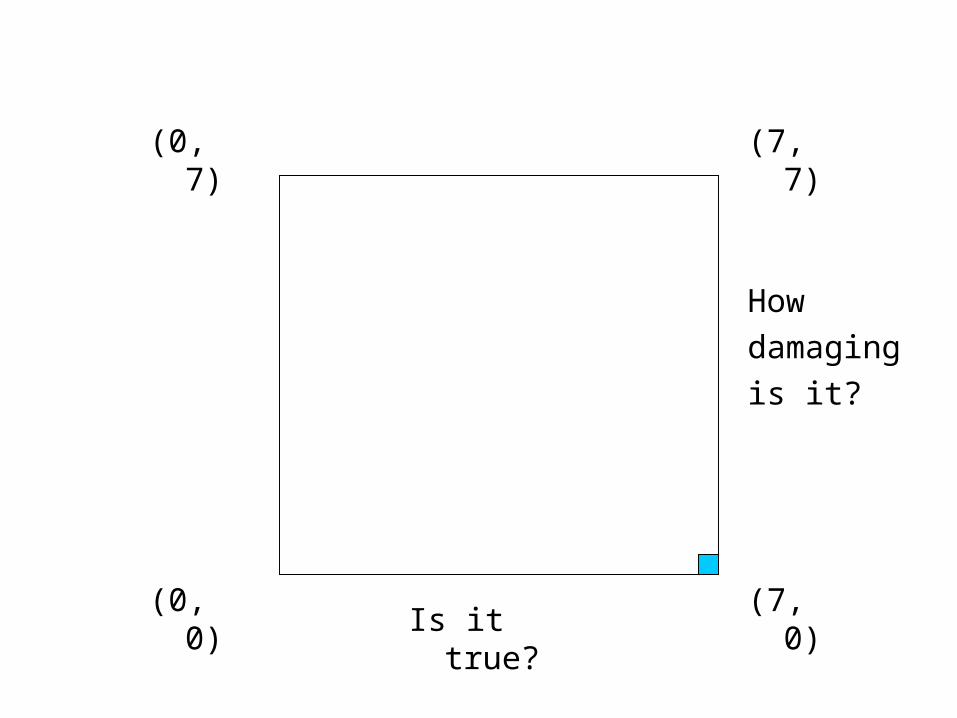
The Financial Hurricane Scale

Example

• The Siberian stock market is a modest but flourishing and competitive regional market

• Interestingly, for the past six years, with 4 exceptions, on the Siberian stock market, stocks have risen every Wednesday and fallen every Thursday

• Furthermore, over the past six years, on all but 3 weekends in which the returns were modest, stocks opened lower on Monday than they closed on Friday.

(0, 0)

(7, 7)

(7, 0)

(0, 7)

Is it true?

How

damaging

is it?

More Examples

• More stocks names begin with the letter ‘x’ than with the letter ‘e’ and their market value is more than 1/26 of the market cap

• There are more than 5 planets in the solar system

(0, 0)

(7, 7)

(7, 0)

(0, 7)

Is it true?

How

damaging

is it?

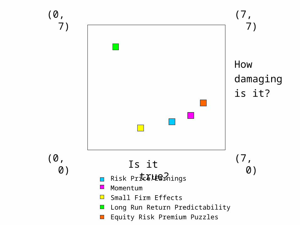
Risk Price/Earnings

Momentum

Small Firm Effects

Long Run Return Predictability

Equity Risk Premium Puzzles

S

(0, 0)

(7, 7)

(7, 0)

(0, 7)

Is it true?

How

damaging

is it?

The Revisionist Behavioral View

• The glass is empty

• Data doesn’t fit the established orthodox views

• The time is ripe for a Kuhn like seismic shift

“Science progresses funeral by funeral”*

*Samuelson

The Behavioral Framework• Investors are a bundle of conflicting emotions:

– Framing – path dependence– Overconfidence – hubris in corporate finance– Too timid?– Irrational in the presence of risk – violate expected

utility and Bayes updating• Investor sentiment is correlated across investors and

random which forces prices ≠ fundamentals• Shifting investor sentiment makes arbitrage risky and

costly and limited• Hence prices are determined by ‘everyman’ and not by the

‘smart’ money

Migration

• Anomalies rarely persist to foster new theories• Typically they migrate westward on the hurricane

scale as the supporting interpretation of the data erodes with replication and statistical analysis

• And typically they migrate south as they yield to neoclassical analysis

• E.G., Long run predictability and the equity premium puzzle

A Modest Proposal• We’re just not as quick as our behavioral

colleagues at coming up with new theories• We use the same theory for many problems

while in the new world of theory you can have one per anomaly

• A moratorium on all empirical work for 5 years to allow the slower neoclassical theorists time to catch up

A Revisionist Theme:Prices Fundamentals

• Unfortunately, ‘fundamentals’ are ambiguous and depend on some pricing theory, e.g., the ‘Internet bubble’

• An exception: closed end funds where fundamentals are unambiguous: fund share price vs. net asset value (NAV)

• We will ‘migrate’ this anomaly

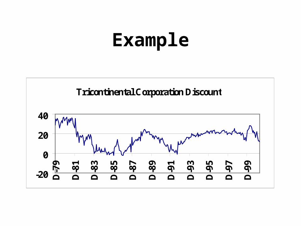
Example

Tricontinental Corporation Discount

-20

0

20

40

D-7

9

D-8

1

D-8

3

D-8

5

D-8

7

D-8

9

D-9

1

D-9

3

D-9

5

D-9

7

D-9

9

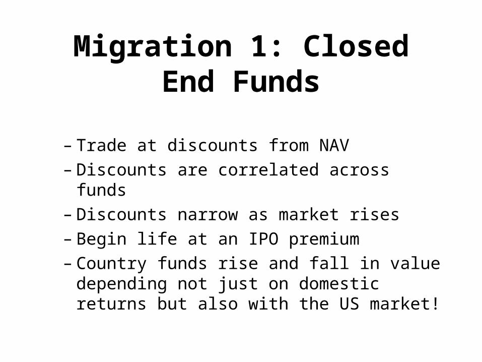
Migration 1: Closed End Funds

– Trade at discounts from NAV– Discounts are correlated across funds– Discounts narrow as market rises– Begin life at an IPO premium– Country funds rise and fall in value depending

not just on domestic returns but also with the US market!

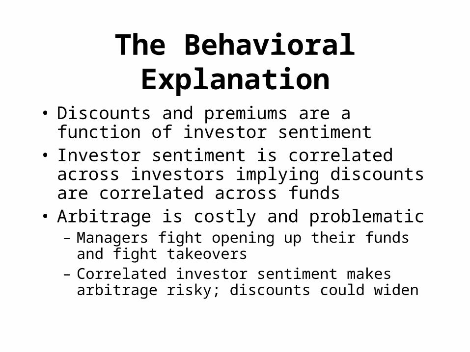
The Behavioral Explanation

• Discounts and premiums are a function of investor sentiment

• Investor sentiment is correlated across investors implying discounts are correlated across funds

• Arbitrage is costly and problematic– Managers fight opening up their funds and fight

takeovers– Correlated investor sentiment makes arbitrage risky;

discounts could widen

Neoclassical Analysis Reprised

• Earlier work (Malkiel [1977])dismissed agency costs, i.e., management fees, taxes, etc.

• But, early analysis used an inappropriate technology to value fees; discounted projected cash flows

• Fees are a derivative on the NAV• An interesting case of scientific sociology;

everyone just quoted the previous papers as ‘proof’ that fees didn’t matter

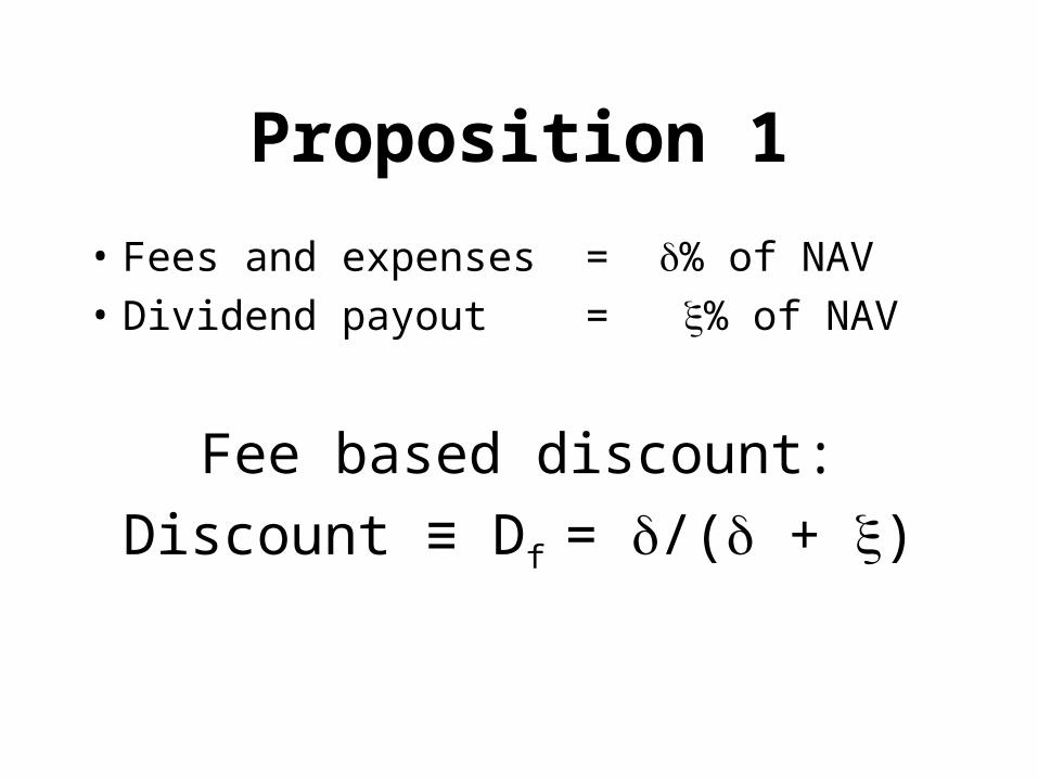
Proposition 1

• Fees and expenses = % of NAV

• Dividend payout = % of NAV

Fee based discount:

Discount ≡ Df = /( + )

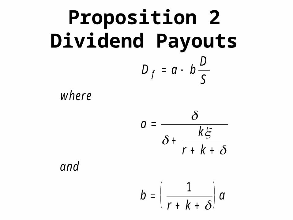
Proposition 2Dividend Payouts

D a bD

Swhere

ak

r kand

br k

a

f

1

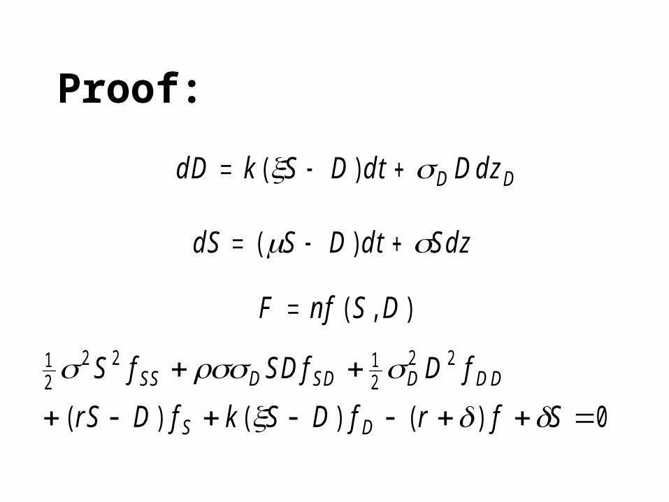
Proof:

12

2 2 12

2 2

0

S f SD f D f

rS D f k S D f r f S

SS D SD D DD

S D

( ) ( ) ( )

dS S D dt Sdz ( )

F nf S D ( , )

dD k S D dt D dzD D ( )

Theory Meets the Data

• The sample average discount:

• 7.7%

• The simple fee based theoretical discount:

• 7.7%

Table 1Fund Theoretical

DiscountTheoretical

DiscountAverageDiscount

ManagementFee

Expenses NAV ($) CapitalGains

Dividends

TickerSymbol

(Expenses)

ADX 0.015 0.015 0.107 0.001 0.003 14.408 0.066 0.029

GAM 0.033 0.031 0.088 0.004 0.009 24.019 0.107 0.017

SBF 0.033 0.032 0.100 0.005 0.005 16.234 0.108 0.027

TY 0.032 0.031 0.130 0.004 0.006 28.601 0.092 0.030

PEO 0.025 0.025 0.068 0.002 0.005 21.568 0.053 0.034

ASA 0.016 0.014 0.074 0.002 0.014 47.511 0.058 0.049

CET 0.013 0.013 0.132 0.001 0.005 17.490 0.078 0.018

JPN 0.044 0.042 0.118 0.006 0.010 13.777 0.120 0.012

SOR 0.074 0.072 0.003 0.008 0.010 39.468 0.020 0.081

MXF 0.239 0.216 0.102 0.011 0.017 15.008 0.015 0.022

ASG 0.091 0.086 0.105 0.007 0.012 11.518 0.048 0.021

FF 0.034 0.033 0.078 0.006 0.010 11.674 0.161 0.011

VLU 0.182 0.156 0.150 0.010 0.019 18.978 0.035 0.010

ZF 0.069 0.066 -0.028 0.007 0.012 11.225 0.007 0.087

USA 0.070 0.068 0.072 0.007 0.010 11.167 0.054 0.039

RVT 0.085 0.081 0.097 0.007 0.012 12.872 0.059 0.016

BLU 0.052 0.051 0.062 0.006 0.009 8.394 0.094 0.015

CLM 0.097 0.086 0.164 0.008 0.017 11.385 0.057 0.014

BZL 0.132 0.118 0.092 0.015 0.029 12.703 0.096 0.002

JEQ 0.078 0.069 -0.052 0.004 0.011 10.338 0.034 0.013

ZSEV 0.203 0.177 -0.048 0.013 0.022 8.289 0.038 0.013

Average 0.077 0.071 0.077 0.006 0.012 17.458 0.067 0.027

The theoretical discounts are calculated by using Proposition 1. The first column of discounts uses only management fees and thesecond adds in total expenses.

Dynamics Payout Rules

• Discount depends on manager/investor split

• The split depends on the payout rule:– A positive feedback from discounts to payouts

– an equilibrium in expectations– Payouts negatively dependent on performance

relative to a benchmark– Payouts designed to maintain a constant NAV

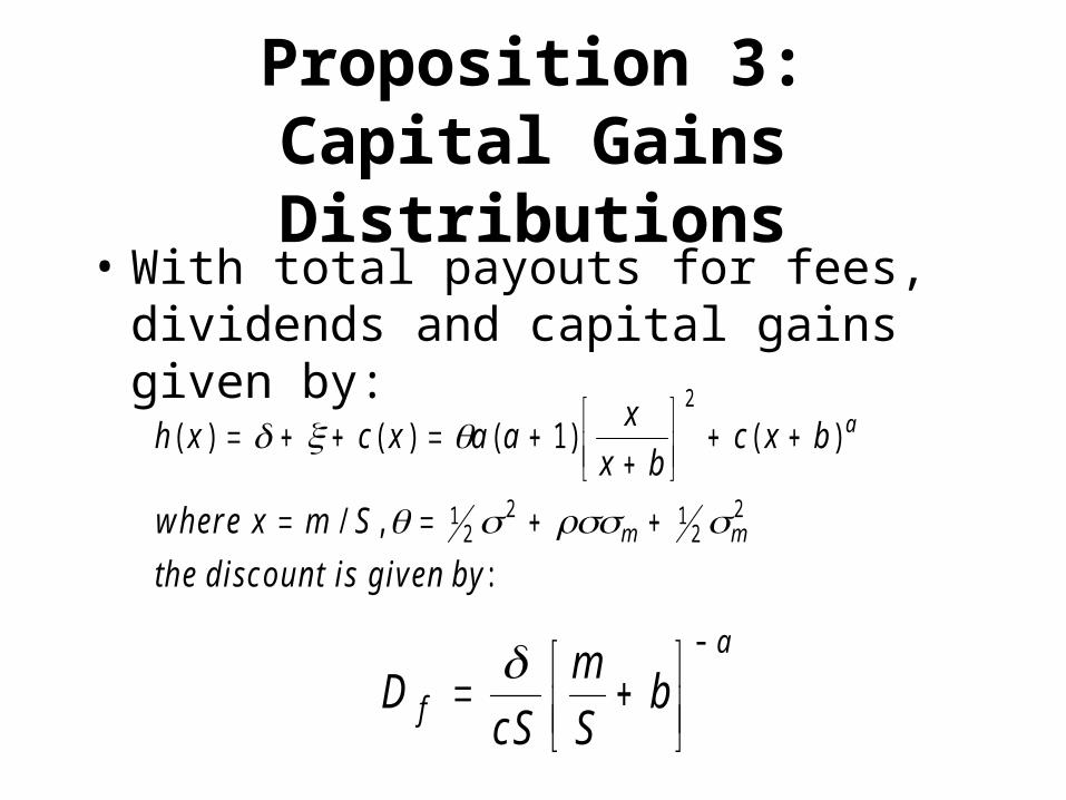
Proposition 3:Capital Gains Distributions

• With total payouts for fees, dividends and capital gains given by:

DcS

m

Sbf

a

h x c x a ax

x bc x b

where x m S

the d iscoun t is g iven by

a

m m

( ) ( ) ( ) ( )

/ ,

:

12

12

2 12

2

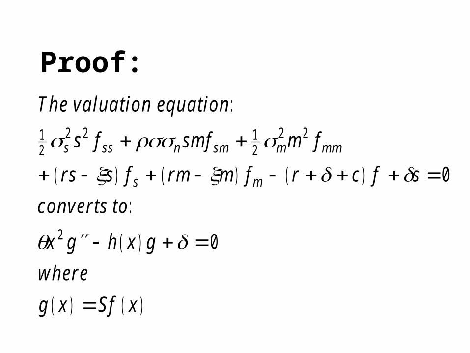
Proof:The va lua tion equa tion

s f sm f m f

rs s f rm m f r c f s

converts to

x g h x g

where

g x S f x

s ss n sm m mm

s m

:

( ) ( ) ( )

:

( )

( ) ( )

12

2 2 12

2 2

2

0

0

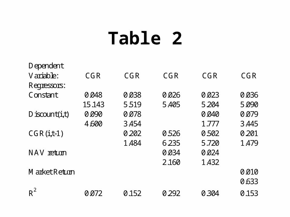
Table 2Dependent Variable: CGR CGR CGR CGR CGRRegressors:Constant 0.048 0.038 0.026 0.023 0.036

15.143 5.519 5.405 5.204 5.090Discount(i,t) 0.090 0.078 0.040 0.079

4.600 3.454 1.777 3.445CGR(i,t-1) 0.202 0.526 0.502 0.201

1.484 6.235 5.720 1.479NAV return 0.034 0.024

2.160 1.432Market Return 0.010

0.633

R2 0.072 0.152 0.292 0.304 0.153

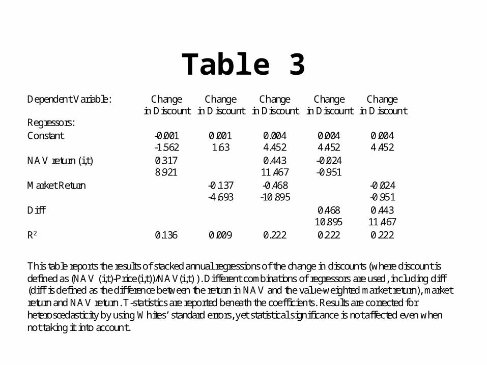
Table 3Dependent Variable: Change Change Change Change Change

in Discount in Discount in Discount in Discount in DiscountRegressors:Constant -0.001 0.001 0.004 0.004 0.004

-1.562 1.63 4.452 4.452 4.452NAV return (i,t) 0.317 0.443 -0.024

8.921 11.467 -0.951Market Return -0.137 -0.468 -0.024

-4.693 -10.895 -0.951Diff 0.468 0.443

10.895 11.467R2 0.136 0.009 0.222 0.222 0.222

This table reports the results of stacked annual regressions of the change in discounts (where discount is defined as (NAV (i,t)-Price(i,t))/NAV(i,t) ). Different combinations of regressors are used, including diff (diff is defined as the difference between the return in NAV and the value-weighted market return), market return and NAV return. T-statistics are reported beneath the coefficients. Results are corrected for heteroscedasticity by using Whites’ standard errors, yet statistical significance is not affected even when not taking it into account.

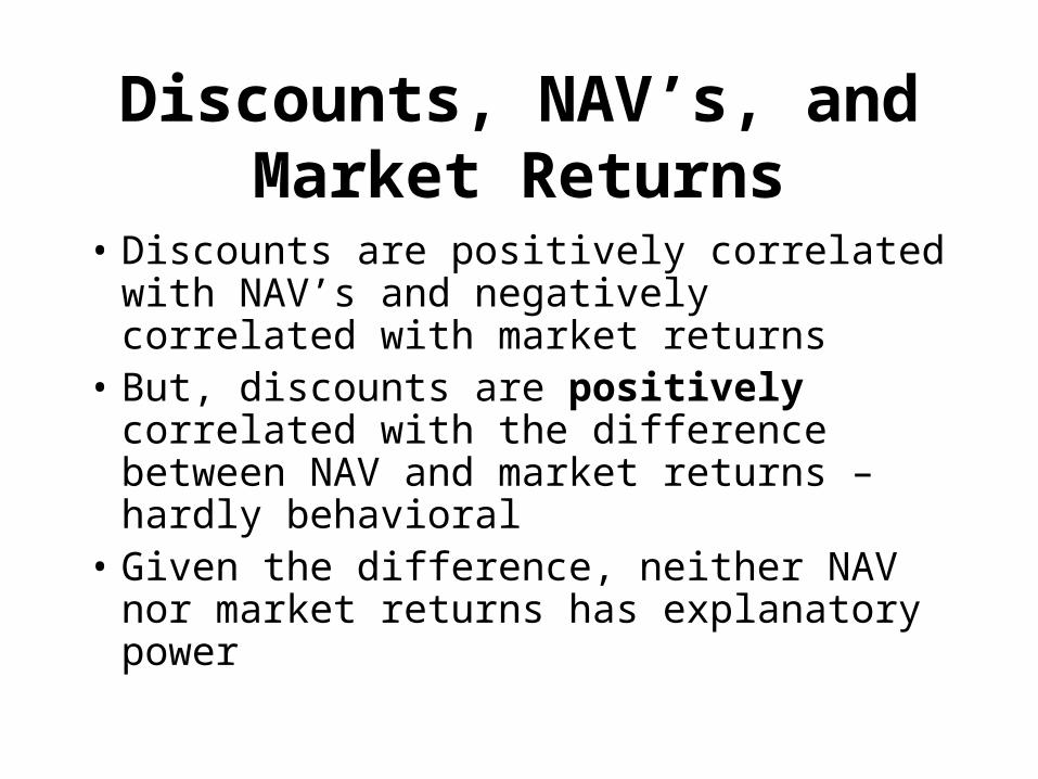
Discounts, NAV’s, and Market Returns

• Discounts are positively correlated with NAV’s and negatively correlated with market returns

• But, discounts are positively correlated with the difference between NAV and market returns – hardly behavioral

• Given the difference, neither NAV nor market returns has explanatory power

The Country Fund Anomaly

• Country funds’ discounts move with the market in which they are traded:

• Capital gains policies depend on the investors’ home market, e.g., payouts are raised when the domestic market is beating the foreign market

• Hence, country fund discounts move with the investors’ home market

Migration 2:Siamese Twins

• Royal Dutch Petroleum (RDP) and Shell Trading and Transport (STT) share in the Group company operating results 60:40

• BUT, their share prices don’t go in a 60:40 lockstep

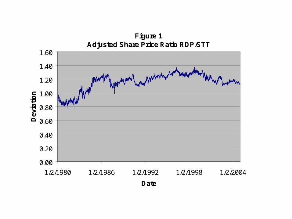
Figure 1

Adjusted Share Price Ratio RDP/STT

0.00

0.20

0.40

0.60

0.80

1.00

1.20

1.40

1.60

1/2/1980 1/2/1986 1/2/1992 1/2/1998 1/2/2004

Date

De

via

tio

n

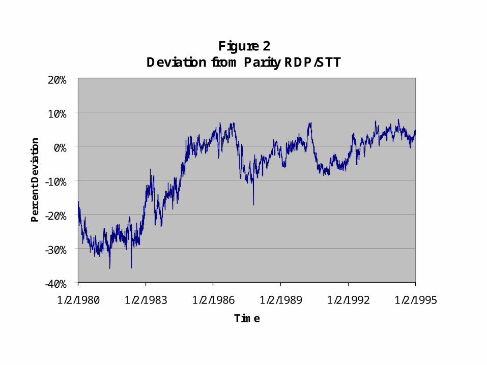
Figure 2

Deviation from Parity RDP/STT

-40%

-30%

-20%

-10%

0%

10%

20%

1/2/1980 1/2/1983 1/2/1986 1/2/1989 1/2/1992 1/2/1995

Time

Pe

rce

nt

De

via

tio

n

Behavioral Analysis

• Irrational noise traders move the price away from parity

• Arbitrage is costly and risky; over long periods the price could deviate further from parity

Neoclassical Analysis

• A true challenge

• Like any good mystery: ‘Follow the cash’

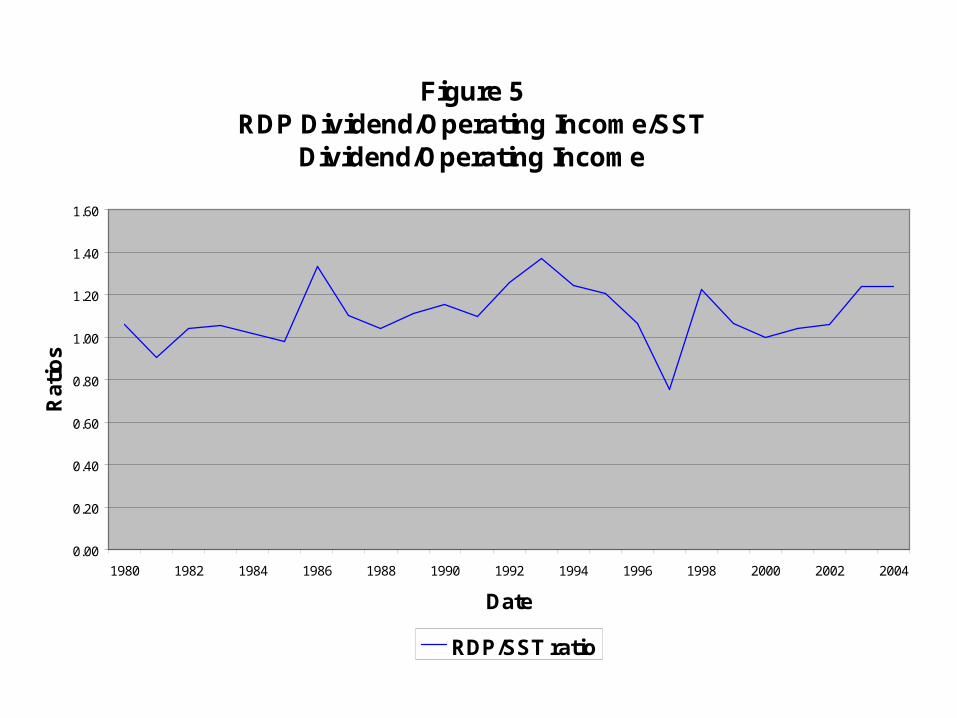
Figure 5RDP Dividend/Operating Income/SST

Dividend/Operating Income

0.00

0.20

0.40

0.60

0.80

1.00

1.20

1.40

1.60

1980 1982 1984 1986 1988 1990 1992 1994 1996 1998 2000 2002 2004

Date

Rat

ios

RDP/SST ratio

Dividends Matter - MM Anew**Siamese Twins Successfully

Separated!?• Volatilities:

– σ(RDP Price/STT Price) = 12%/year– σ(RDP Dividend/STT Dividend) = 14%/year

• MM: How can dividends matter? Changing the timing of payouts doesn’t change firm value

• But, changing the level of payouts does• If the dividends leave ‘value at infinity’ then

raising them will raise value– Example: A firm has one million krona of government

bonds, but only pays a dividend of one krona/year

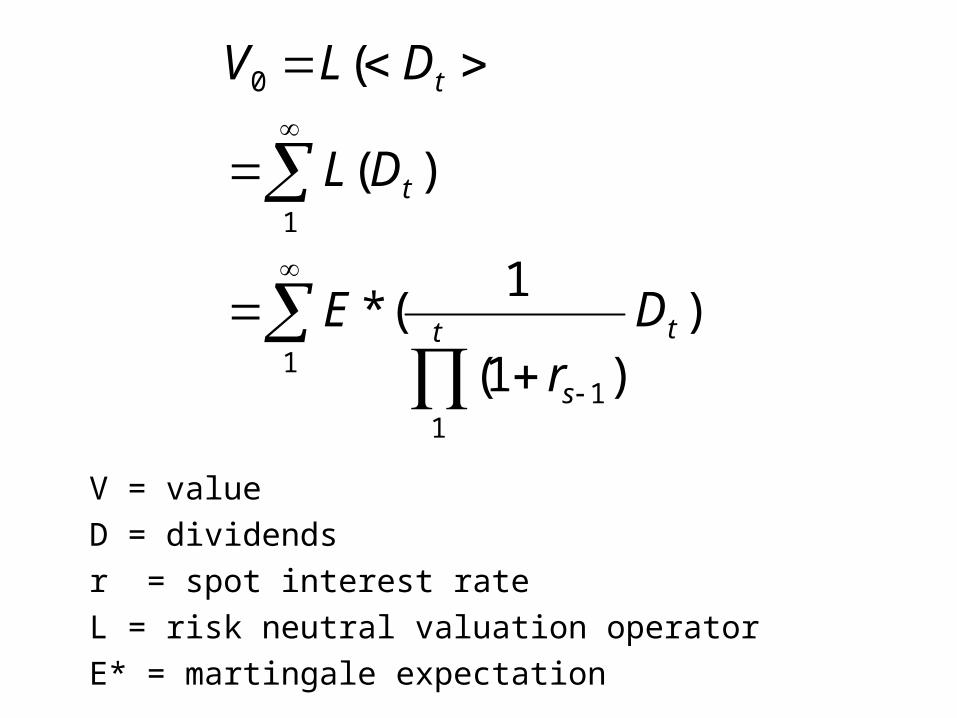
V = value

D = dividends

r = spot interest rate

L = risk neutral valuation operator

E* = martingale expectation

1

11

1

0

))1(

1(*

)(

(

tt

s

t

t

Dr

E

DL

DLV

t

s

t

st

ttt

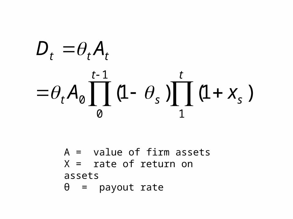
xA

AD

1

1

00 )1()1(

A = value of firm assetsX = rate of return on assetsθ = payout rate

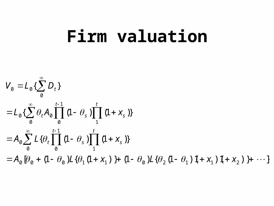
Firm valuation

])}1)(1)(1({)1()}1({)1([

})1()1({

})1()1({

}{

2112011000

0 1

1

00

0 1

1

000

000

xxLxLA

xLA

xAL

DLV

t

s

t

st

t

s

t

st

t

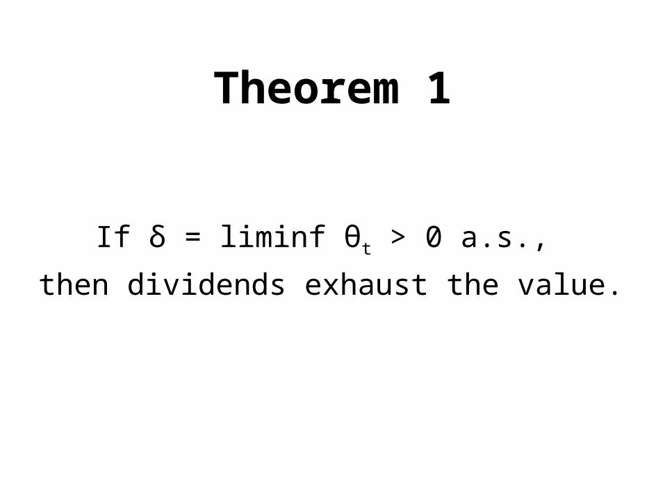
Theorem 1

If δ = liminf θt > 0 a.s.,

then dividends exhaust the value.

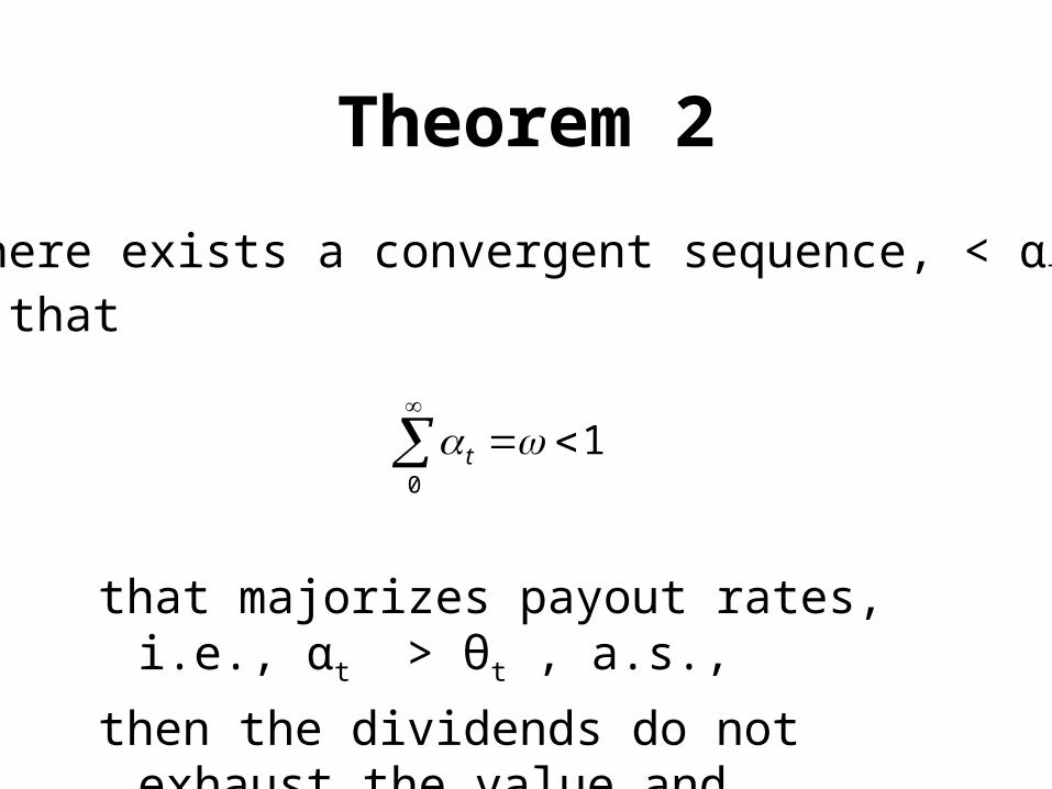
Theorem 2

If there exists a convergent sequence, < αt > ,such that

10

t

that majorizes payout rates, i.e., αt > θt , a.s.,

then the dividends do not exhaust the value and

there is value at infinity.

Bubbles

• Value at infinity is a form of a ‘rational’ bubble• Rational bubbles occur when the myopic valuation

equation is solved for an arbitrary positive value at infinity which produces an arbitrary current value

• By contrast, we set the price equal to the discounted payouts and identify the remaining value as locked in the firm presumably because of imperfections in corporate control

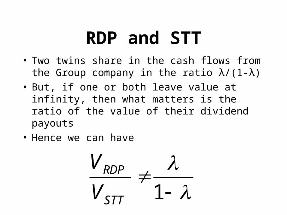
RDP and STT• Two twins share in the cash flows from the Group

company in the ratio λ/(1-λ)• But, if one or both leave value at infinity, then

what matters is the ratio of the value of their dividend payouts

• Hence we can have

1STT

RDP

V

V

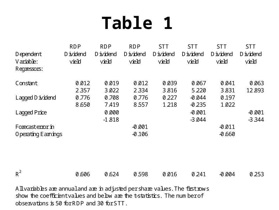
Table 1

Dependent Variable:

RDP Dividend

yield

RDP Dividend

yield

RDP Dividend

yield

STT Dividend

yield

STT Dividend

yield

STT Dividend

yield

STT Dividend

yieldRegressors:

Constant 0.012 0.019 0.012 0.039 0.067 0.041 0.0632.357 3.022 2.334 3.816 5.220 3.831 12.893

Lagged Dividend 0.776 0.708 0.776 0.227 -0.044 0.1978.650 7.419 8.557 1.218 -0.235 1.022

Lagged Price 0.000 -0.001 -0.001-1.818 -3.044 -3.344

Forecast error in -0.001 -0.011Operating Earnings -0.106 -0.660

R2 0.606 0.624 0.598 0.016 0.241 -0.004 0.253

All variables are annual and are in adjusted per share values. The first rowsshow the coefficient values and below are the t-statistics. The number ofobservations is 50 for RDP and 30 for STT.

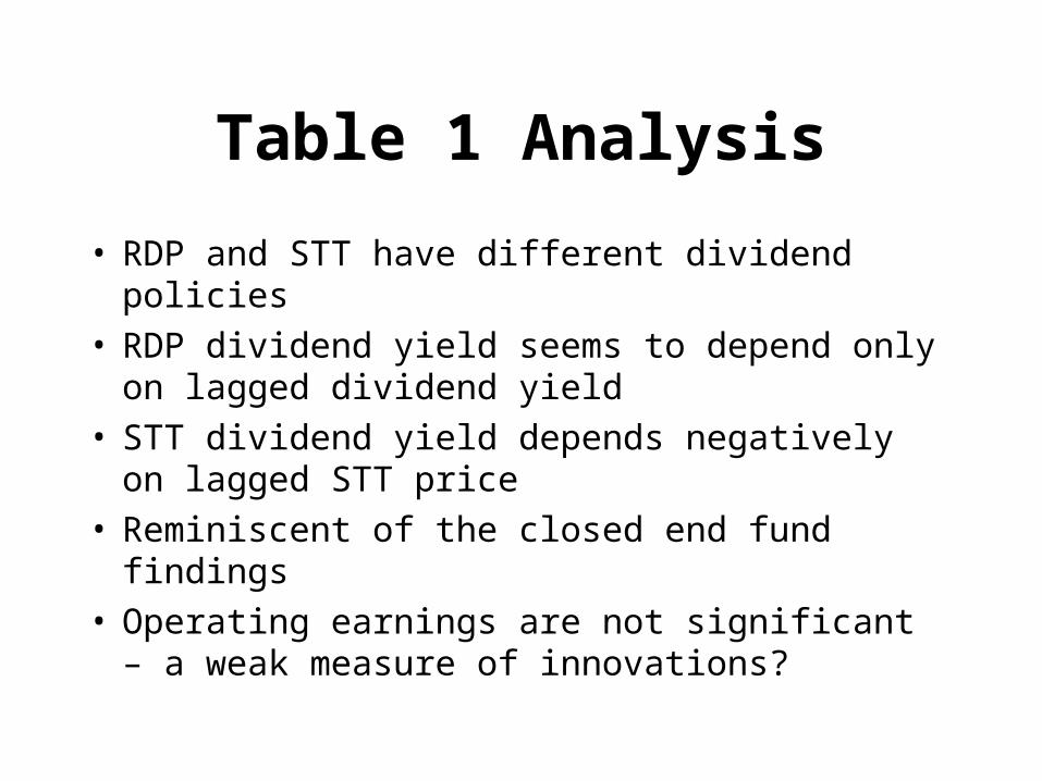
Table 1 Analysis

• RDP and STT have different dividend policies• RDP dividend yield seems to depend only on

lagged dividend yield• STT dividend yield depends negatively on lagged

STT price• Reminiscent of the closed end fund findings• Operating earnings are not significant – a weak

measure of innovations?

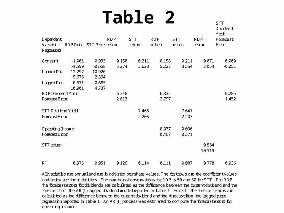
Table 2Dependent Variable: RDP Price STT Price

RDP return

STT return

RDP return

STT return

RDP return

STT Dividend Yield Forecast Error

Regressors:

Constant -1.001 -0.933 0.158 0.211 0.158 0.211 0.071 0.000-1.590 -0.658 5.274 3.623 5.227 3.554 3.054 -0.051

Lagged Dividend12.297 10.9265.676 2.394

Lagged Price 0.671 0.68510.001 4.737

RDP Dividend Yield 6.316 6.332 0.285Forecast Error 2.813 2.797 1.452

STT Dividend Yield 7.465 7.641Forecast Error 2.205 2.203

Operating Income 0.077 0.096Forecast Error 0.467 0.371

STT return 0.58410.119

R2 0.975 0.951 0.126 0.114 0.111 0.087 0.778 0.036

All variables are annual and are in adjusted per share values. The first rows are the coefficient valuesand below are the r-statistics. The number of observations for RDP is 50 and 30 for STT. For RDPthe forecast errors for dividends are calculated as the difference between the current dividend and theforecast from the AR(1) lagged dividend model reported in Table 1. For STT the forecast errors are calculated as the difference between the current dividend and the forecast from the lagged price regression reported in Table 1. An AR(1) process was estimated to compute the forecast errors foroperating income.

Table 2 Analysis

• Dividend innovations are insignificantly correlated – returns are strongly correlated

• Prices depend significantly on lagged dividends in the presence of lagged prices

• Given dividend yield innovations, operating earnings are irrelevant

• Returns for each company are correlated with contemporaneous dividend innovations

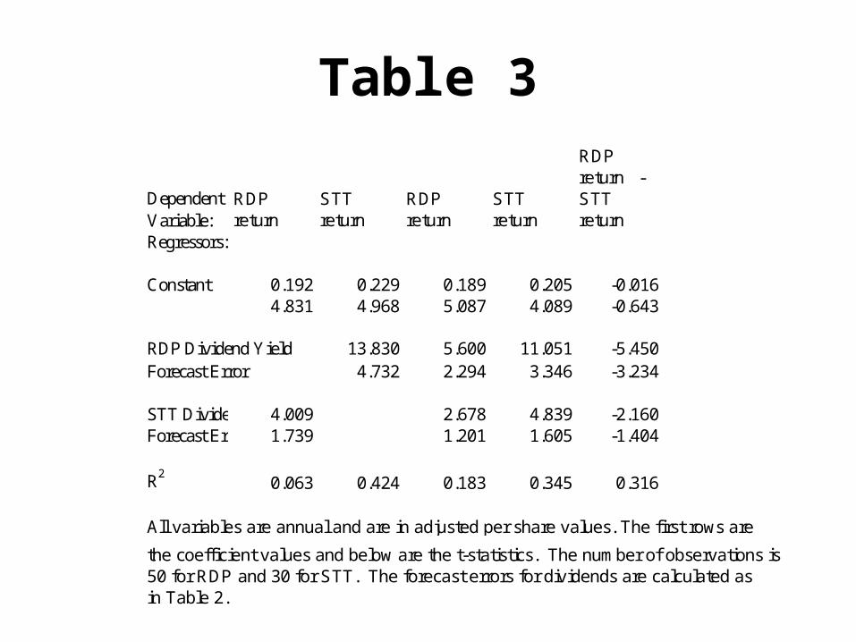
Table 3

Dependent Variable:

RDP return

STT return

RDP return

STT return

RDP return - STT return

Regressors:

Constant 0.192 0.229 0.189 0.205 -0.0164.831 4.968 5.087 4.089 -0.643

RDP Dividend Yield 13.830 5.600 11.051 -5.450Forecast Error 4.732 2.294 3.346 -3.234

STT Dividend Yield4.009 2.678 4.839 -2.160Forecast Error 1.739 1.201 1.605 -1.404

R20.063 0.424 0.183 0.345 0.316

All variables are annual and are in adjusted per share values. The first rows are

the coefficient values and below are the t-statistics. The number of observations is50 for RDP and 30 for STT. The forecast errors for dividends are calculated as in Table 2.

Table 3 Analysis

• Innovations in the RDP dividend yield significantly affect RDP and STT returns

• STT dividend yield innovations have no explanatory power for RDP returns

• RDP - STT returns is inversely dependent on RDP dividend yield innovations

• As with a closed end fund, STT must raise dividends to raise its value to compete with RDP?

Summary:Neoclassical vs. Behavioral

• Parsimony vs. ad hocery– NA and market efficiency produce the answer

• Psychology offers too many answers– Are people optimists or pessimists – they are both

• Neoclassical theory predicts the magnitude as well as the signs of effects

• Aesthetics; I prefer theories with some distance between assumptions and conclusions– You want correlations, presto! Assume correlated

individual irrational behavior

A Skeptic’s Perspective on the Role of Psychology in Finance

• Psychology is currently a grab bag of fascinating anecdotes and observations begging for theory

• When added to NA and efficiency, it has little to offer for price determination

• Psychology may have value for financial marketing and the flows of funds – although the value added over empirical economics is not clear

Conclusion

• Finance has unsolved problems

• Thank God for that!

• Unfortunately, though, so far it looks as though we will have to solve them ourselves