A Nested Dissection Approach to Sparse Matrix Partitioning ...egboman/papers/ND-SISC.pdf · A NESTED DISSECTION APPROACH TO SPARSE MATRIX PARTITIONING FOR PARALLEL COMPUTATIONS

A NESTED DISSECTION APPROACH TO SPARSE MATRIXPARTITIONING FOR PARALLEL COMPUTATIONS

ERIK G. BOMAN∗ AND MICHAEL M. WOLF†

Abstract. We consider how to distribute sparse matrices among processes to reduce com-munication costs in parallel sparse matrix computations, specifically, sparse matrix-vector multi-plication. Our main contributions are: (i) an exact graph model for communication with general(two-dimensional) matrix distribution, and (ii) a recursive partitioning algorithm based on nesteddissection (substructuring). We show that the communication volume is closely linked to vertexseparators.

We have implemented our algorithm using hypergraph partitioning software to enable a faircomparison with existing methods. We present numerical results for sparse matrices from severalapplication areas, with up to 9 million nonzeros. The results show that our new approach is superiorto traditional 1d partitioning and comparable to a current leading partitioning method, the fine-grain hypergraph method, in terms of communication volume. Our nested dissection method hastwo advantages over the fine-grain method: it is faster to compute, and the resulting distributionrequires fewer communication messages.

Keywords: Parallel data distributions, sparse matrix computations, graph par-titioning, nested dissection, matrix-vector multiplication.

AMS subject classifications. 05C50, 05C85, 65F50, 65Y05, 68R10

1. Introduction. Sparse matrix-vector multiplication (SpMV) is a common ker-nel in many computations, e.g., iterative solvers for linear systems of equations andPageRank computation (power method) for ranking web pages. Often the same ma-trix is used for many iterations. An important combinatorial problem in parallel com-puting is how to distribute the matrix and the vectors among processes to minimizethe communication cost. Such “communication” is also important on serial computerswith deep memory hierarchies, where slow memory is typically much slower than fastmemory. Since CPU performance increases more rapidly than memory, we expectmemory latency and bandwith to grow in importance. Our present work is relevantto both parallel computation on distributed memory computers and serial computa-tion on machines with hierarchical memory, but we phrase our work in the context ofparallel computing. Our work also applies to Jacobi and Gauss-Seidel iterations andthe more general computation y = F (x), where x is an input vector, y is an outputvector, and F is a sparse (possibly nonlinear) operator that is “decomposable” suchthat partial evaluations can be computed independently and then combined.

Sparse matrix-vector multiplication y = Ax is usually parallelized such that theprocess that owns element aij computes the contribution aijxj . This is a local op-eration if xj , yi and aij all reside on the same process; otherwise communication isrequired. In general, the following four steps are performed [7, 21]:

1. Expand: Send entries xj to processes with a nonzero aij for some i.2. Local multiply-add: yi := yi + aijxj .3. Fold: Send partial y values to relevant processes.

∗Scalable Algorithms Dept, Sandia National Labs, Albuquerque, NM 87185-1318,[email protected]. Sandia is a multiprogram laboratory operated by Sandia Corporation,a Lockheed Martin Company, for the DOE’s National Nuclear Security Administration undercontract number DE-AC-94AL85000.

†Dept. of Computer Science, Univ. of Illinois at Urbana-Champaign, [email protected], andScalable Algorithms Dept, Sandia National Labs.

1

2 ERIK G. BOMAN AND MICHAEL M. WOLF

4. Sum: Sum up the partial y values.In this paper, we address sparse matrix-vector partitioning, where both the ma-

trix nonzeros and vector elements are partitioned into different parts. For parallelcomputing, this data is mapped to different processes based on this part assignment.

Definition 1.1. Sparse matrix-vector partitioning: Given a sparse matrix A,an integer k > 1, and ε > 0, compute

(i) a matrix partition A =∑k

i=1 Ai where each Ai contains a subset of the nonze-ros of A, such that nnz(Ai) ≤ (1 + ε)nnz(A)/k, ∀i, where nnz denotes thenumber of nonzeros,

(ii) partitions of the input and output vectors,such that when the data is distributed across processes based on these partitions, thecommunication volume in sparse matrix-vector multiply, y = Ax, is minimized.

This problem is NP-hard since it contains as a special case hypergraph partition-ing. Stated above is a very general form. We first consider a special version forsymmetric matrices where the input and output vectors must have the same distri-bution. It has been observed [7, 4] that the matrix and vector partitioning problemscan be separated. For any given matrix distribution (partition), it is easy to finda “compatible” vector partition and these together give a solution to the combinedmatrix-vector problem. Additional objectives can be minimized in the vector par-titioning phase [4, 5]. We focus on the matrix partitioning step but simultaneouslyobtain a compatible vector partitioning as well.

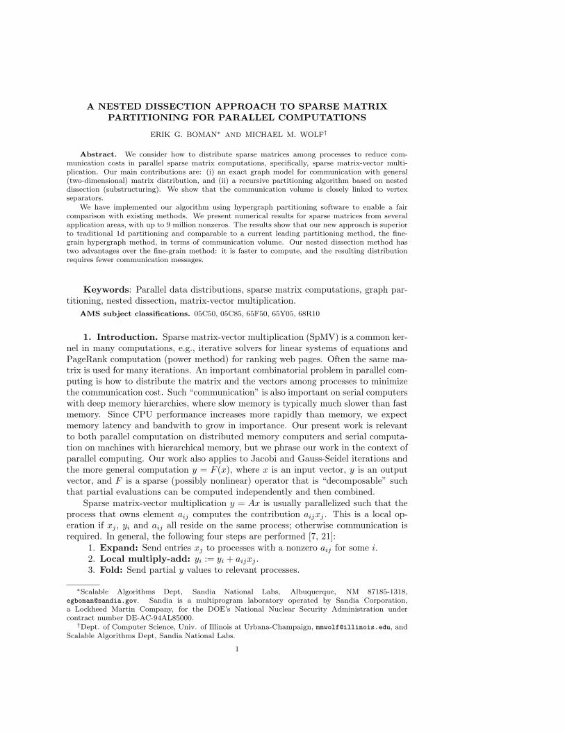
By far, the most common way to partition a sparse matrix is to use a 1d schemewhere each part is assigned the nonzeros for a set of rows or columns. This approachhas two advantages: simplicity for the user and only one communication phase (nottwo). The simplest 1d method is to assign ≈ n/k consecutive rows (or columns)to each part, where n denotes the number of rows and k the number of parts in apartition (Figure 1.1). However, it is often possible to reduce the communication bypartitioning the rows in a better (non-contiguous) way, using graphs, bipartite graphs,or hypergraphs to model this problem (Subsections 2.1 - 2.3) [16, 7].

Fig. 1.1. 1d row and column partitioning of a matrix. Each color denotes a part that is assigneda different process.

Recently, several 2d decompositions have been proposed [8, 21]. The idea isto reduce the communication volume further by giving up the simplicity of the 1dstructure. The fine-grain distribution [8] is of particular interest since it is the mostgeneral and is theoretically optimal (though not in practice). We introduce a graphmodel that also accurately describes communication in fine-grain distribution. Thisleads to a new graph-based algorithm, a “nested dissection partitioning algorithm,”which we describe in Section 4. (A preliminary version, without analysis, appearedin [6].) This nested dissection partitioning algorithm is related to previous nesteddissection work for parallel Cholesky factorization [14, 15]. An important aspect toboth our partitioning method and the previous parallel Cholesky factorization workis that communication is limited to separator vertices in the corresponding graph.

The rest of this paper is organized as follows. In Section 2 we discuss 1d and

NESTED DISSECTION APPROACH TO SPARSE MATRIX PARTITIONING 3

2d data distribution, while in Section 3 we present a new graph model for symmetricpartitioning. In Section 4 we present an algorithm based on this model, and inSection 5 we discuss the nonsymmetric case. We present numerical results in Section 6that validate our approach.

2. Background: 1d and 2d Distributions.

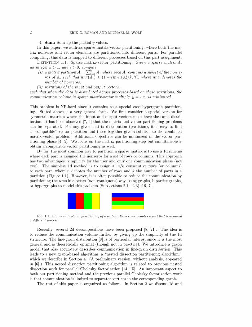
2.1. 1d Graph Model. The standard graph model is limited to structurallysymmetric matrices. In this case, the graph G is defined such that the adjacencymatrix of G has the same nonzero pattern as the matrix A. Each row (or column) inA corresponds to a vertex in G. A partitioning of the vertices in G gives a partitioningof the rows (columns) in A. The standard objective is to minimize the number ofcut edges, but this does not accurately reflect communication volume. Figure 2.1illustrates this. Twice the number of cut edges (highlighted in magenta) yields acommunication volume of 6 words, which overcounts the correct volume of 4 words.The problem is that vertices 1 and 8 are counted twice in the metric but each onlycontributes one word to the volume. The communication required is associated withthe boundary vertices, so a better metric is to minimize the boundary vertices (4words for Figure 2.1, which is correct). This is an exact metric for bisection, whilefor k > 2 one should also take into account the number of adjacent parts.

3

45

6

12

7

1 873 542 61

32

87654

8

Fig. 2.1. 1d graph partitioning of matrix into two parts. Correct communication volume is 4words. Communication of highlighted vertices is overcounted in edge metric.

2.2. 1d Bipartite Graph Model. The graph model works poorly on nonsym-metric square matrices because they need be symmetrized, and does not apply torectangular matrices. The bipartite graph model was designed to rectify this [16].The bipartite graph G = (R,C,E) is defined such that vertices R correspond to rows,vertices C correspond to columns, and edges E correspond to nonzeros. The standard(simplest) objective is to partition both R and C such that the number of cut edges isminimized. Only one of the vertex partitionings (either R for rows, or C for columns)is used to obtain a 1d matrix partitioning. Again, the cut edges do not correctly countcommunication volume, and boundary vertices should be used instead.

2.3. 1d Hypergraph Model. Aykanat and Catalyurek introduced the hyper-graph model to count communication volume accurately [7]. A hypergraph generalizesa graph. Whereas a graph edge contains exactly two vertices, a hyperedge can con-tain an arbitrary set of vertices [2, 3]. There are two 1d hypergraph models. Inthe row-net model, each column is a vertex and each row a hyperedge, while in thecolumn-net model, each row is a vertex and each column a hyperedge. The objectiveis to find a balanced vertex partitioning and minimize the number of cut hyperedges.The communication volume is

∑i(λi−1), where λi is the number of parts that touch


hyperedge i. Finding the optimal balanced vertex partitioning is NP-hard but inpractice good partitions can be found in (near-linear) polynomial time [7].

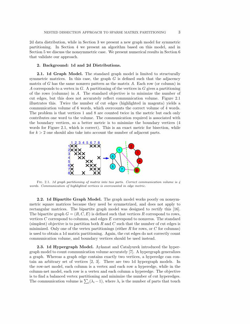
2.4. 2d Matrix Distributions. Although the simplicity of 1d distributionsmay be desirable, the communication volume can often be reduced by using 2d dis-tributions. Figure 2.2 shows an example where 1d partitioning will always be poor.Consider the arrowhead matrix of dimension n, and bisection (k = 2). Due to a singledense row and column, any load balanced 1d partitioning will have a communicationvolume of approximately (3/4)n words. The optimal volume is actually 2 words asdemonstrated in the 2d partitioning of Figure 2.2 (right).

Fig. 2.2. Arrowhead matrix with 1d (left) and 2d (right) distribution, for two parts (red andblue). The communication volumes in this example are eight and two words, respectively.

2.5. Current 2d Methods. Two-dimensional partitioning is a more flexible al-ternative to one-dimensional partitioning. For dense matrices, it was realized that a 2dblock (checkerboard) distribution reduces communication since communication is lim-ited to process rows and columns. For sparse matrices, the situation is more complex.Several algorithms have been proposed to take advantage of the flexibility affordedby a two-dimensional partitioning but none have become dominant. Catalyurek andAykanat proposed both a fine-grain [8] and a coarse-grain [9] decomposition, whileBisseling and Vastenhouw later developed the Mondriaan method [21]. The coarse-grain method is similar to the 2d block (checkerboard) decomposition in the densecase, but is difficult to compute (requires multiconstraint hypergraph partitioning)and often gives relatively high communication volume. The fine-grain method giveslow communication volume but is also expensive to compute. The Mondriaan methodtries to find a middle ground. It is based on recursive 1d hypergraph partitioning andthus is relatively fast but still produces partitions with low communication cost.

The most flexible approach to matrix partitioning is to allow any nonzero to beassigned any part. This is the idea underlying the fine-grain method [8]. The authorspropose a hypergraph model that exactly represents communication volume. In thefine-grain hypergraph model, each nonzero corresponds to a vertex, and each row andeach column corresponds to a hyperedge. A matrix A with m rows, n colums, and znonzeros yields a hypergraph with z vertices and m + n hyperedges. Catalyurek andAykanat proved that this fine-grain hypergraph model yields a minimum volume parti-tion when optimally solved [8]. As with the 1d hypergraph model, finding the optimalpartition of the fine-grain model is NP-hard. This hypergraph can be partitioned intok approximately equal parts cutting few hyperedges using standard one-dimensionalpartitioning algorithms and software. This usually takes significantly longer than aone-dimensional partitioning of a typical matrix since the fine-grain hypergraph islarger than a 1d hypergraph model of the original matrix. However, there is specialstructure in this hypergraph (each vertex is incident to exactly two hyperedges) that


1 873 542 61

32

876543

4

56

1 2

7 8

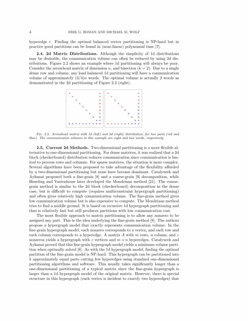
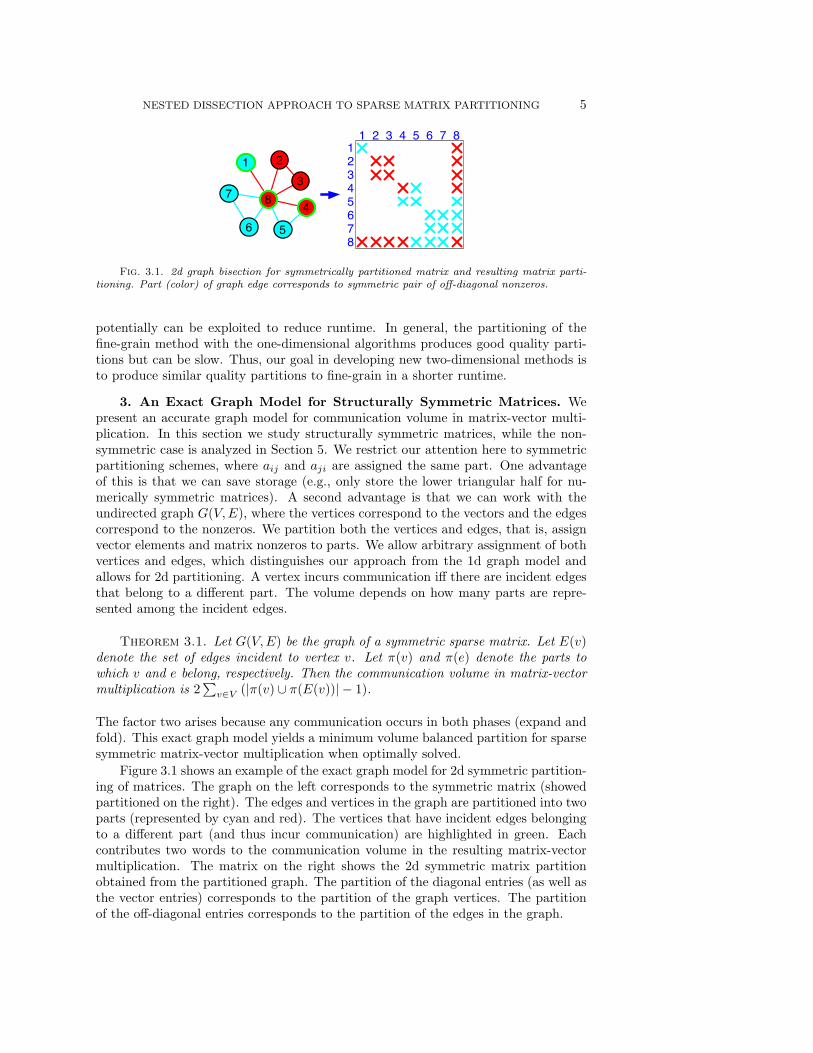
Fig. 3.1. 2d graph bisection for symmetrically partitioned matrix and resulting matrix parti-tioning. Part (color) of graph edge corresponds to symmetric pair of off-diagonal nonzeros.

potentially can be exploited to reduce runtime. In general, the partitioning of thefine-grain method with the one-dimensional algorithms produces good quality parti-tions but can be slow. Thus, our goal in developing new two-dimensional methods isto produce similar quality partitions to fine-grain in a shorter runtime.

3. An Exact Graph Model for Structurally Symmetric Matrices. Wepresent an accurate graph model for communication volume in matrix-vector multi-plication. In this section we study structurally symmetric matrices, while the non-symmetric case is analyzed in Section 5. We restrict our attention here to symmetricpartitioning schemes, where aij and aji are assigned the same part. One advantageof this is that we can save storage (e.g., only store the lower triangular half for nu-merically symmetric matrices). A second advantage is that we can work with theundirected graph G(V,E), where the vertices correspond to the vectors and the edgescorrespond to the nonzeros. We partition both the vertices and edges, that is, assignvector elements and matrix nonzeros to parts. We allow arbitrary assignment of bothvertices and edges, which distinguishes our approach from the 1d graph model andallows for 2d partitioning. A vertex incurs communication iff there are incident edgesthat belong to a different part. The volume depends on how many parts are repre-sented among the incident edges.

Theorem 3.1. Let G(V,E) be the graph of a symmetric sparse matrix. Let E(v)denote the set of edges incident to vertex v. Let π(v) and π(e) denote the parts towhich v and e belong, respectively. Then the communication volume in matrix-vectormultiplication is 2

∑v∈V (|π(v) ∪ π(E(v))| − 1).

The factor two arises because any communication occurs in both phases (expand andfold). This exact graph model yields a minimum volume balanced partition for sparsesymmetric matrix-vector multiplication when optimally solved.

Figure 3.1 shows an example of the exact graph model for 2d symmetric partition-ing of matrices. The graph on the left corresponds to the symmetric matrix (showedpartitioned on the right). The edges and vertices in the graph are partitioned into twoparts (represented by cyan and red). The vertices that have incident edges belongingto a different part (and thus incur communication) are highlighted in green. Eachcontributes two words to the communication volume in the resulting matrix-vectormultiplication. The matrix on the right shows the 2d symmetric matrix partitionobtained from the partitioned graph. The partition of the diagonal entries (as well asthe vector entries) corresponds to the partition of the graph vertices. The partitionof the off-diagonal entries corresponds to the partition of the edges in the graph.


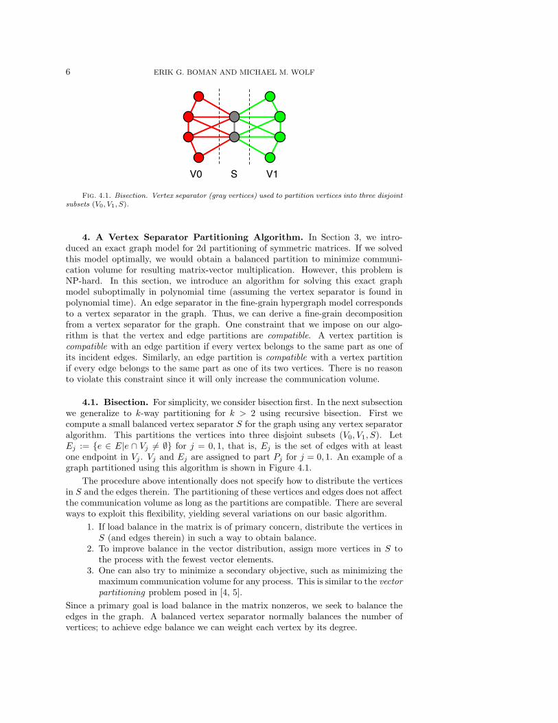
V0 S V1

Fig. 4.1. Bisection. Vertex separator (gray vertices) used to partition vertices into three disjointsubsets (V0, V1, S).

4. A Vertex Separator Partitioning Algorithm. In Section 3, we intro-duced an exact graph model for 2d partitioning of symmetric matrices. If we solvedthis model optimally, we would obtain a balanced partition to minimize communi-cation volume for resulting matrix-vector multiplication. However, this problem isNP-hard. In this section, we introduce an algorithm for solving this exact graphmodel suboptimally in polynomial time (assuming the vertex separator is found inpolynomial time). An edge separator in the fine-grain hypergraph model correspondsto a vertex separator in the graph. Thus, we can derive a fine-grain decompositionfrom a vertex separator for the graph. One constraint that we impose on our algo-rithm is that the vertex and edge partitions are compatible. A vertex partition iscompatible with an edge partition if every vertex belongs to the same part as one ofits incident edges. Similarly, an edge partition is compatible with a vertex partitionif every edge belongs to the same part as one of its two vertices. There is no reasonto violate this constraint since it will only increase the communication volume.

4.1. Bisection. For simplicity, we consider bisection first. In the next subsectionwe generalize to k-way partitioning for k > 2 using recursive bisection. First wecompute a small balanced vertex separator S for the graph using any vertex separatoralgorithm. This partitions the vertices into three disjoint subsets (V0, V1, S). LetEj := {e ∈ E|e ∩ Vj 6= ∅} for j = 0, 1, that is, Ej is the set of edges with at leastone endpoint in Vj . Vj and Ej are assigned to part Pj for j = 0, 1. An example of agraph partitioned using this algorithm is shown in Figure 4.1.

The procedure above intentionally does not specify how to distribute the verticesin S and the edges therein. The partitioning of these vertices and edges does not affectthe communication volume as long as the partitions are compatible. There are severalways to exploit this flexibility, yielding several variations on our basic algorithm.

1. If load balance in the matrix is of primary concern, distribute the vertices inS (and edges therein) in such a way to obtain balance.

2. To improve balance in the vector distribution, assign more vertices in S tothe process with the fewest vector elements.

3. One can also try to minimize a secondary objective, such as minimizing themaximum communication volume for any process. This is similar to the vectorpartitioning problem posed in [4, 5].

Since a primary goal is load balance in the matrix nonzeros, we seek to balance theedges in the graph. A balanced vertex separator normally balances the number ofvertices; to achieve edge balance we can weight each vertex by its degree.


4.1.1. Analysis of Separator Assignment. For a minimal separator S, eachvertex in S must have at least one non-separator neighbor in V0 and one in V1. Weassume this to be the case for the (possibly non-minimal) separator used in our al-gorithm. This is a reasonable assumption since otherwise a smaller separator couldbe trivially obtained by moving the problematic vertex to the set of its non-separatorneighbor vertex, and most vertex separator implementations would do this. Commu-nication in SpMV is limited to the vertices in S. This follows from the above methodof assigning all edges that have at least one non-separator vertex to the part of thisnon-separator vertex, such that each non-separator vertex is only incident to edges ofits part. Thus, non-separator vertices do not incur communication.

Lemma 4.1. Suppose S is a separator where each vertex in S has at least onenon-separator neighbor in V0 and one in V1. Then the communication in SpMV islimited to the vertices in S, and the volume is 2|S|. Furthermore, the assignment ofvertices in S and edges therein does not matter as long as compatibility is maintained.

Proof. Each vertex in S is incident to at least one edge assigned to P0 and oneedge assigned to P1. Thus, the part assignment of the edges connecting vertices in Sdoes not affect the communication volume. Each separator vertex will incur 1 wordof communication for each phase whether it is assigned to P0 or P1. Thus, the com-munication volume is exactly |S| in each phase or 2|S| total.

Theorem 4.2. For bisection, the vertex separator partitioning algorithm with aminimal balanced vertex separator minimizes communication volume in sparse matrix-vector multiplication (for a balanced partition).

Proof. Since each vertex incurring communication (in bisection) incurs 1 word ofcommunication (in each phase), finding the minimum set of vertices that incur com-munication will minimize the communication in matrix-vector multiplication. Thisminimum set of vertices is the minimum vertex separator.

This shows that the vertex separator method is optimal for k = 2, just like thefine-grain hypergraph method.

4.2. Nested Dissection Partitioning Algorithm. In practice, one wishes topartition into k > 2 parts. If we knew a method to compute a balanced k-separator, aset S such that the removal of S breaks G into k disjoint subgraphs, we could assigneach subgraph to a different part. However, we do not know efficient methods tocompute a k-separator and do not consider this option any further. A more practicalapproach is to use recursive bisection. In fact, the procedure to compute a k−separatorvia recursive bisection is known as “nested dissection” and well studied [13, 19] sinceit is important for sparse matrix factorization.

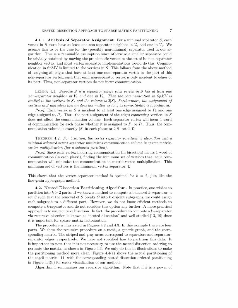
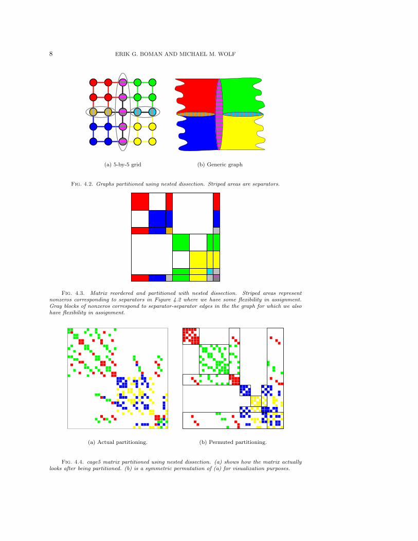
The procedure is illustrated in Figures 4.2 and 4.3. In this example there are fourparts. We show the recursive procedure on a mesh, a generic graph, and the corre-sponding matrix. The striped and gray areas correspond to separators and separator-separator edges, respectively. We have not specified how to partition this data. Itis important to note that it is not necessary to use the nested dissection ordering topermute the matrix, as shown in Figure 4.3. We only do this in illustrations to makethe partitioning method more clear. Figure 4.4(a) shows the actual partitioning ofthe cage5 matrix [11] with the corresponding nested dissection ordered partitioningin Figure 4.4(b) for easier visualization of our method.

Algorithm 1 summarizes our recursive algorithm. Note that if k is a power of


(a) 5-by-5 grid (b) Generic graph

Fig. 4.2. Graphs partitioned using nested dissection. Striped areas are separators.

Fig. 4.3. Matrix reordered and partitioned with nested dissection. Striped areas representnonzeros corresponding to separators in Figure 4.2 where we have some flexibility in assignment.Gray blocks of nonzeros correspond to separator-separator edges in the the graph for which we alsohave flexibility in assignment.

(a) Actual partitioning. (b) Permuted partitioning.

Fig. 4.4. cage5 matrix partitioned using nested dissection. (a) shows how the matrix actuallylooks after being partitioned. (b) is a symmetric permutation of (a) for visualization purposes.


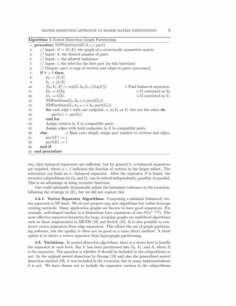
Algorithm 1 Nested Dissection Graph Partitioning1: procedure NDPartition(G, k, ε, i, part)2: // Input: G = (V,E), the graph of a structurally symmetric matrix3: // Input: k, the desired number of parts4: // Input: ε, the allowed imbalance5: // Input: i, the label for the first part (in this bisection)6: // Output: part, a map of vertices and edges to parts (processes)7: if k > 1 then8: k0 := dk/2e9: k1 := bk/2c

10: [V0, V1, S] := sep(G, k0/k, ε/(log k))) . Find balanced separator.11: G0 := G|V0 . G restricted to V0

12: G1 := G|V1 . G restricted to V1

13: NDPartition(G0, k0, ε, i, part(G0))14: NDPartition(G1, k1, ε, i + k0, part(G1))15: for each edge e with one endpoint, v, in V0 or V1 but not the other do16: part(e) := part(v)17: end for18: Assign vertices in S to compatible parts19: Assign edges with both endpoints in S to compatible parts20: else . Base case; simply assign part number to vertices and edges.21: part(V ) := i22: part(E) := i23: end if24: end procedure

two, then balanced separators are sufficient, but for general k, α-balanced separatorsare required, where α < 1 indicates the fraction of vertices in the larger subset. Thesubroutine sep finds an α−balanced separator. After the separator S is found, therecursive subproblems for G0 and G1 can be solved independently, possibly in parallel.This is an advantage of using recursive bisection.

One could optionally dynamically adjust the imbalance tolerance in the recursion,following the strategy in [21], but we did not explore this.

4.2.1. Vertex Separator Algorithms. Computing a minimal (balanced) ver-tex separator is NP-hard. We do not propose any new algorithms but rather leverageexisting methods. Many application graphs are known to have good separators. Forexample, well-shaped meshes in d dimensions have separators of size O(n1−1/d). Themost effective separator heuristics for large, irregular graphs are multilevel algorithmssuch as those implemented in METIS [18] and Scotch [10]. It is also possible to con-struct vertex separators from edge separators. This allows the use of graph partition-ing software, but the quality is often not as good as a more direct method. A thirdoption is to derive a vertex separator from hypergraph partitioning.

4.3. Variations. In nested dissection algorithms, there is a choice how to handlethe separator at each level. Say V has been partitioned into V0, V1, and S, where Sis the separator. The question is whether S should be included in the subproblems ornot. In the original nested dissection by George [13] and also the generalized nesteddissection method [19], it was included in the recursion, but in many implementationsit is not. We have chosen not to include the separator vertices in the subproblems


in the recursion since it simplified our implementation. A complication for us is thatif the separator is not included, additional rules are needed to decide how to assignvertices and edge adjacent to the separators. However, this can be advantageous ifthis flexibility is used properly. We also found it useful to formulate a slightly moregeneral non-recursive algorithm, which has the following steps:

1. Compute non-overlapping separators. This yields k disjoint subdomains di-vided by a hierarchy of k − 1 separators.

2. Let Vi be the vertices in the subdomain i. Assign the vertices in Vi to partPi.

3. Let Ei be the edges that contain a vertex in Vi. Assign the edges in Ei to Pi.4. Assign separator vertices to parts.5. Assign edges connecting vertices of the same separator to parts.6. Assign edges connecting vertices of two different separators to parts. By

design these separators will be at different levels.The algorithm does not depend on any particular method for calculating the vertexseparators in step 1. However, in general, smaller separators will tend to yield lowercommunication volumes. Steps 2 and 3 are fully expounded in the description above.However, there are many different ways to do the part assignment in steps 4-6 andwe leave this decision to the particular implementation.

In our initial implementation, we assign all the vertices in a given separator (step4) to a part in the range of parts belonging to one half of the subdomain. The halfis chosen to keep the vertex partitioning as balanced as possible. We assigned eachseparator vertex (step 4) to the part of the first traversed neighbor vertex in the correctrange that had already been assigned a part. This greedy heuristic can be improvedbut had the advantage of being simple to implement and yielding better results thansome more complicated heuristics. For the part assignment of edges interior to aseparator (step 5), we assigned these edges to the part of the lowered numbered ofthe two vertices. We assigned edges connecting vertices from two different separators(step 6) to the part of the vertex of the lower-level separator. There were two reasonsfor this choice: It is consistent with Algorithm 1, and empirically it yielded betterresults. The rules in steps 4-6 are reasonable but not always optimal, so there maybe room for improvement.

4.4. Communication Volume Analysis. For our analysis of our implementa-tion, we assume that the number of parts is a power of two (k = 2i). It follows thatthere are k− 1 separators. We number the separators S1, S2, . . . , Sk−1 in order of thelevel of the separators. We define S to be the union of the separators (S =

⋃k−1i=1 Si)

and know that⋂k−1

i=1 Si = ∅ since the separators are non-overlapping. We show lowerand upper bounds on the communication volume, Vol.

Theorem 4.3. The communication volume in SpMV with partitioning producedby Algorithm 1 satisfies Vol(G, k) ≥ 2|S|.

Proof. Each separator vertex vs ∈ S is connected to edges of at least two differentparts. Thus, for any partitioning of vs, vs will incur at least one word of communica-tion for each of the two communication phases.

It is important to note that this bound is valid for the general algorithm as well asour particular implementation.

Theorem 4.4. The communication volume in SpMV with partitioning produced


by our implementation outlined in Subsection 4.3 satisfies

Vol(G, k) ≤ 2k−1∑i=1

|Si|(

k

2blog2 ic − 1)

.

Proof. With our implementation choice of assigning edges connecting verticesfrom two different separators to the part of the lower level separator, a separatorvertex does not incur communication from its connection with higher level separatorvertices. Thus, a given separator vertex vs of separator Si can be incident to edges ofat most k

2blog2 ic different parts since the edge partition is compatible with the vertexpartition. Thus, vs incurs at most k

2blog2 ic − 1 words of communication for each com-munication phase.

It is important to note that this bound does not apply to the general nested dissectionpartitioning algorithm (step steps above) but for our slightly more specific algorithm(Algorithm 1) that assigns edges connecting vertices from two different separators thepart of the lower level separator. Without this edge partitioning rule, our bound wouldnot be as tight (Vol(G, k) ≤ 2

∑k−1i=1 |Si| (k − 1)). This justifies our implementation

choice.

4.5. Relation to Nested Dissection for Parallel Cholesky Factorization.As previously mentioned, the dissection partitioning algorithm presented in this sec-tion is related to previous nested dissection work for parallel Cholesky factorization[14, 15]. The elimination tree used in Cholesky factorization is equivalent to a treethat can be formed from our hierarchy of separators and with the non-separator ver-tices as leaves of the tree. Also in both usages of nested dissection, communication islimited to separator vertices in the corresponding graph.

However, there are a few important distinctions between the partitioning for par-allel Cholesky factorization and our partitioning for parallel matrix-vector multiplica-tion. In parallel Cholesky, the elimination tree represents dependency constraints inthe elimination order, but there are no such dependency constraints in matrix-vectormultiplication. Also in the parallel Cholesky factorization work, there are additionalfill nonzeros to take into account (and to partition) but no such additional nonzerosoccur in our partitioning for matrix-vector multiplication. Related to this, permutingthe matrix is important to Cholesky in order to reduce the fill. For our objective ofreducing communication volume in matrix-vector multiplication, it is not importantto impose the nested dissection ordering on the matrix since vertex orderings will haveno effect on the communication volume. Also, the parallel Cholesky factorization as-sumes that the nonzeros in each column of lower triangular L will be assigned to oneprocess (1d partitioning). This column partitioning with subtree task assignment willbe a special case of the partitioning allowed in our general matrix partitioning algo-rithm. We do not specify that the separator-separator blocks (gray blocks in Figure4.3) are partitioned in this column-wise manner and thus allow for a 2d partitioningof the lower triangular portion of the matrix.

5. Nonsymmetric Case. The undirected graph model is limited to structurallysymmetric graphs. In the nonsymmetric case, we can use a directed graph or abipartitite graph. First we show how we can apply our nested dissection partitioningalgorithm to bipartite graphs to partition nonsymmetric matrices. Then we discussprevious related work of the doubly bordered block diagonal (DBBD) form.


11

2

2

3

3

4

4 5

5

6 7

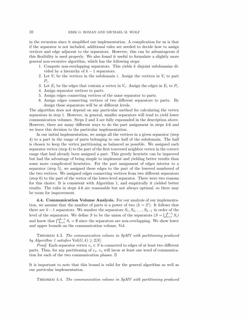
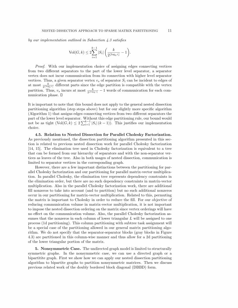
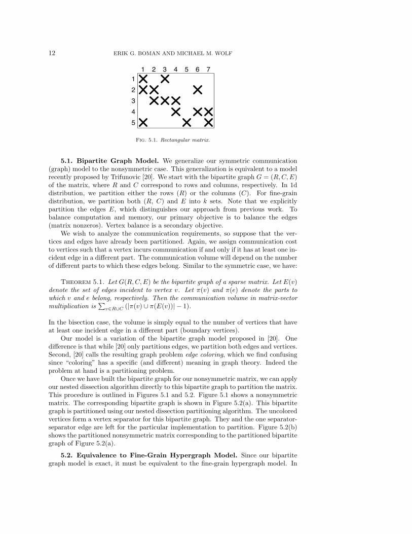
Fig. 5.1. Rectangular matrix.

5.1. Bipartite Graph Model. We generalize our symmetric communication(graph) model to the nonsymmetric case. This generalization is equivalent to a modelrecently proposed by Trifunovic [20]. We start with the bipartite graph G = (R,C, E)of the matrix, where R and C correspond to rows and columns, respectively. In 1ddistribution, we partition either the rows (R) or the columns (C). For fine-graindistribution, we partition both (R, C) and E into k sets. Note that we explicitlypartition the edges E, which distinguishes our approach from previous work. Tobalance computation and memory, our primary objective is to balance the edges(matrix nonzeros). Vertex balance is a secondary objective.

We wish to analyze the communication requirements, so suppose that the ver-tices and edges have already been partitioned. Again, we assign communication costto vertices such that a vertex incurs communication if and only if it has at least one in-cident edge in a different part. The communication volume will depend on the numberof different parts to which these edges belong. Similar to the symmetric case, we have:

Theorem 5.1. Let G(R,C, E) be the bipartite graph of a sparse matrix. Let E(v)denote the set of edges incident to vertex v. Let π(v) and π(e) denote the parts towhich v and e belong, respectively. Then the communication volume in matrix-vectormultiplication is

∑v∈R∪C (|π(v) ∪ π(E(v))| − 1).

In the bisection case, the volume is simply equal to the number of vertices that haveat least one incident edge in a different part (boundary vertices).

Our model is a variation of the bipartite graph model proposed in [20]. Onedifference is that while [20] only partitions edges, we partition both edges and vertices.Second, [20] calls the resulting graph problem edge coloring, which we find confusingsince “coloring” has a specific (and different) meaning in graph theory. Indeed theproblem at hand is a partitioning problem.

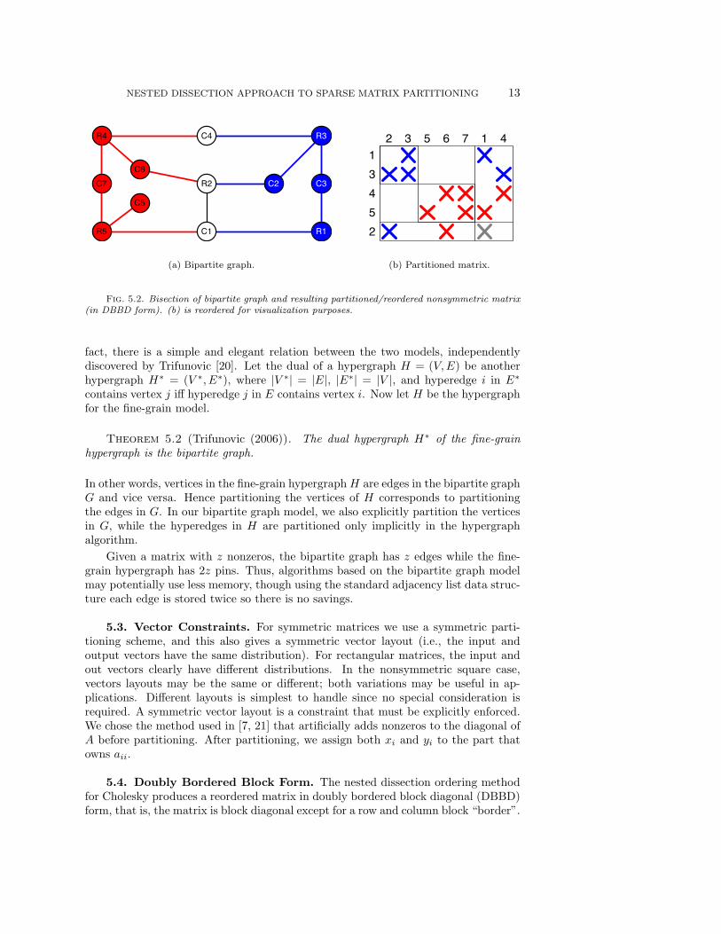
Once we have built the bipartite graph for our nonsymmetric matrix, we can applyour nested dissection algorithm directly to this bipartite graph to partition the matrix.This procedure is outlined in Figures 5.1 and 5.2. Figure 5.1 shows a nonsymmetricmatrix. The corresponding bipartite graph is shown in Figure 5.2(a). This bipartitegraph is partitioned using our nested dissection partitioning algorithm. The uncoloredvertices form a vertex separator for this bipartite graph. They and the one separator-separator edge are left for the particular implementation to partition. Figure 5.2(b)shows the partitioned nonsymmetric matrix corresponding to the partitioned bipartitegraph of Figure 5.2(a).

5.2. Equivalence to Fine-Grain Hypergraph Model. Since our bipartitegraph model is exact, it must be equivalent to the fine-grain hypergraph model. In


R2

C1

C4R4

R5

C5

C6C7

R1

R3

C2 C3

(a) Bipartite graph.

1

2

345

12 3 45 6 7

(b) Partitioned matrix.

Fig. 5.2. Bisection of bipartite graph and resulting partitioned/reordered nonsymmetric matrix(in DBBD form). (b) is reordered for visualization purposes.

fact, there is a simple and elegant relation between the two models, independentlydiscovered by Trifunovic [20]. Let the dual of a hypergraph H = (V,E) be anotherhypergraph H∗ = (V ∗, E∗), where |V ∗| = |E|, |E∗| = |V |, and hyperedge i in E∗

contains vertex j iff hyperedge j in E contains vertex i. Now let H be the hypergraphfor the fine-grain model.

Theorem 5.2 (Trifunovic (2006)). The dual hypergraph H∗ of the fine-grainhypergraph is the bipartite graph.

In other words, vertices in the fine-grain hypergraph H are edges in the bipartite graphG and vice versa. Hence partitioning the vertices of H corresponds to partitioningthe edges in G. In our bipartite graph model, we also explicitly partition the verticesin G, while the hyperedges in H are partitioned only implicitly in the hypergraphalgorithm.

Given a matrix with z nonzeros, the bipartite graph has z edges while the fine-grain hypergraph has 2z pins. Thus, algorithms based on the bipartite graph modelmay potentially use less memory, though using the standard adjacency list data struc-ture each edge is stored twice so there is no savings.

5.3. Vector Constraints. For symmetric matrices we use a symmetric parti-tioning scheme, and this also gives a symmetric vector layout (i.e., the input andoutput vectors have the same distribution). For rectangular matrices, the input andout vectors clearly have different distributions. In the nonsymmetric square case,vectors layouts may be the same or different; both variations may be useful in ap-plications. Different layouts is simplest to handle since no special consideration isrequired. A symmetric vector layout is a constraint that must be explicitly enforced.We chose the method used in [7, 21] that artificially adds nonzeros to the diagonal ofA before partitioning. After partitioning, we assign both xi and yi to the part thatowns aii.

5.4. Doubly Bordered Block Form. The nested dissection ordering methodfor Cholesky produces a reordered matrix in doubly bordered block diagonal (DBBD)form, that is, the matrix is block diagonal except for a row and column block “border”.


For example, with two diagonal blocks we have the structureA11 0 A13

0 A22 A23

A31 A32 A33

.

A key insight is that communication is limited to these borders, both for Choleskyand SpMV. Aykanat et al. [1] showed DBBD form for a nonsymmetric matrix can beobtained by computing a vertex separator in the bipartite graph. We can use this inthe following way. Given a nonsymmetric possibly rectangular matrix (see Figure 5.1),form the bipartite graph (Figure 5.2(a)). Perform a nonsymmetric nested dissectionordering where the row and column vertices in the separator are ordered last. Thisgives a permuted matrix (Figure 5.2(b)) that can be partitioned according to the samerules as in the symmetric case. Note that as before, in practice it is not necessary todo the permutation (but is helpful in the illustration).

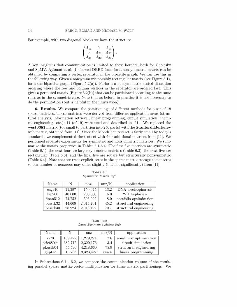
6. Results. We compare the partitionings of different methods for a set of 19sparse matrices. These matrices were derived from different application areas (struc-tural analysis, information retrieval, linear programming, circuit simulation, chemi-cal engineering, etc.); 14 (of 19) were used and described in [21]. We replaced thewest0381 matrix (too small to partition into 256 parts) with the Stanford Berkeleyweb matrix, obtained from [11]. Since the Mondriaan test set is fairly small by today’sstandards, we complemented the test set with four additional matrices from [11]. Weperformed separate experiments for symmetric and nonsymmetric matrices. We sum-marize the matrix properties in Tables 6.1-6.4. The first five matrices are symmetric(Table 6.1), the next four are larger symmetric matrices (Table 6.2), the next five arerectangular (Table 6.3), and the final five are square but structurally nonsymmetric(Table 6.4). Note that we treat explicit zeros in the sparse matrix storage as nonzerosso our number of nonzeros may differ slightly (but not significantly) from [11].

Table 6.1Symmetric Matrix Info

Name N nnz nnz/N applicationcage10 11,397 150,645 13.2 DNA electrophoresislap200 40,000 200,000 5.0 2-D Laplacian

finan512 74,752 596,992 8.0 portfolio optimizationbcsstk32 44,609 2,014,701 45.2 structural engineeringbcsstk30 28,924 2,043,492 70.7 structural engineering

Table 6.2Large Symmetric Matrix Info

Name N nnz nnz/N applicationc-73 169,422 1,279,274 7.6 non-linear optimization

asic680ks 682,712 2,329,176 3.4 circuit simulationpkustk04 55,590 4,218,660 75.9 structural engineeringgupta3 16,783 9,323,427 555.5 linear programming

In Subsections 6.1 - 6.2, we compare the communication volume of the result-ing parallel sparse matrix-vector multiplication for these matrix partitionings. We


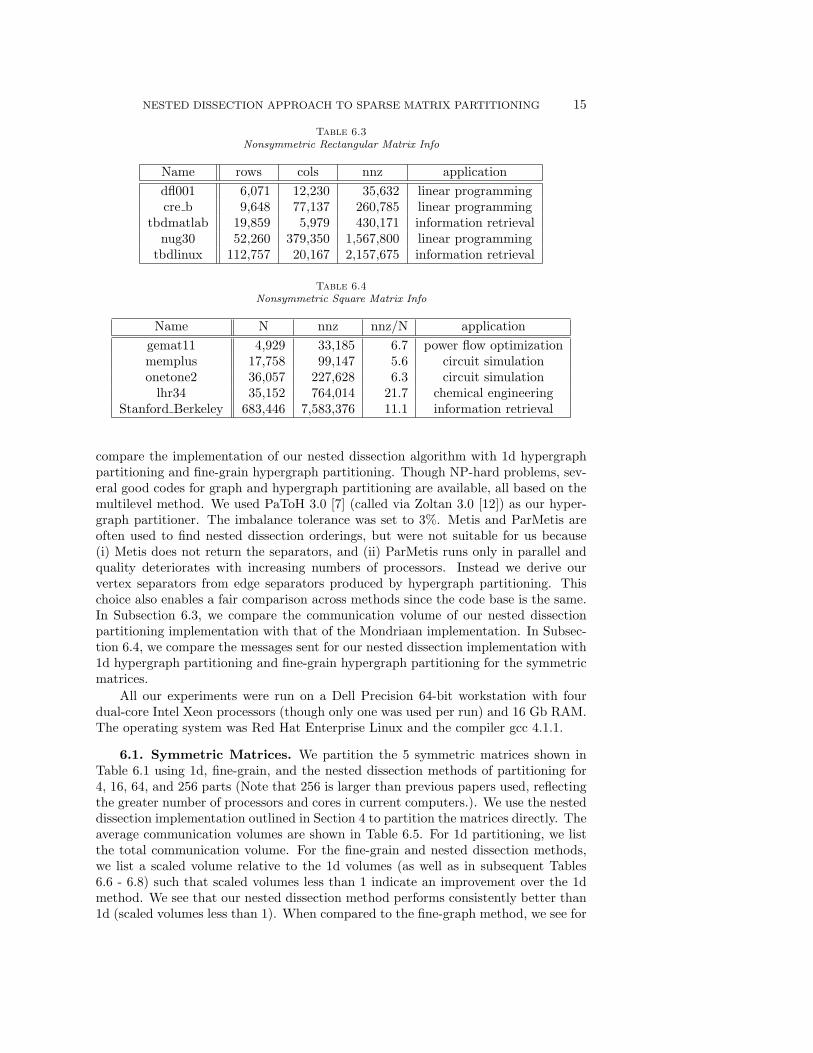
Table 6.3Nonsymmetric Rectangular Matrix Info

Name rows cols nnz applicationdfl001 6,071 12,230 35,632 linear programmingcre b 9,648 77,137 260,785 linear programming

tbdmatlab 19,859 5,979 430,171 information retrievalnug30 52,260 379,350 1,567,800 linear programming

tbdlinux 112,757 20,167 2,157,675 information retrieval

Table 6.4Nonsymmetric Square Matrix Info

Name N nnz nnz/N applicationgemat11 4,929 33,185 6.7 power flow optimizationmemplus 17,758 99,147 5.6 circuit simulationonetone2 36,057 227,628 6.3 circuit simulation

lhr34 35,152 764,014 21.7 chemical engineeringStanford Berkeley 683,446 7,583,376 11.1 information retrieval

compare the implementation of our nested dissection algorithm with 1d hypergraphpartitioning and fine-grain hypergraph partitioning. Though NP-hard problems, sev-eral good codes for graph and hypergraph partitioning are available, all based on themultilevel method. We used PaToH 3.0 [7] (called via Zoltan 3.0 [12]) as our hyper-graph partitioner. The imbalance tolerance was set to 3%. Metis and ParMetis areoften used to find nested dissection orderings, but were not suitable for us because(i) Metis does not return the separators, and (ii) ParMetis runs only in parallel andquality deteriorates with increasing numbers of processors. Instead we derive ourvertex separators from edge separators produced by hypergraph partitioning. Thischoice also enables a fair comparison across methods since the code base is the same.In Subsection 6.3, we compare the communication volume of our nested dissectionpartitioning implementation with that of the Mondriaan implementation. In Subsec-tion 6.4, we compare the messages sent for our nested dissection implementation with1d hypergraph partitioning and fine-grain hypergraph partitioning for the symmetricmatrices.

All our experiments were run on a Dell Precision 64-bit workstation with fourdual-core Intel Xeon processors (though only one was used per run) and 16 Gb RAM.The operating system was Red Hat Enterprise Linux and the compiler gcc 4.1.1.

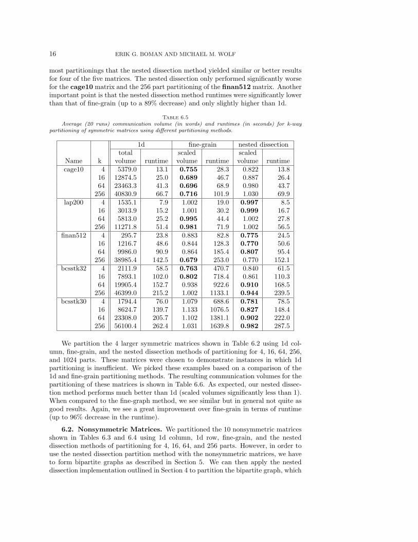
6.1. Symmetric Matrices. We partition the 5 symmetric matrices shown inTable 6.1 using 1d, fine-grain, and the nested dissection methods of partitioning for4, 16, 64, and 256 parts (Note that 256 is larger than previous papers used, reflectingthe greater number of processors and cores in current computers.). We use the nesteddissection implementation outlined in Section 4 to partition the matrices directly. Theaverage communication volumes are shown in Table 6.5. For 1d partitioning, we listthe total communication volume. For the fine-grain and nested dissection methods,we list a scaled volume relative to the 1d volumes (as well as in subsequent Tables6.6 - 6.8) such that scaled volumes less than 1 indicate an improvement over the 1dmethod. We see that our nested dissection method performs consistently better than1d (scaled volumes less than 1). When compared to the fine-graph method, we see for


most partitionings that the nested dissection method yielded similar or better resultsfor four of the five matrices. The nested dissection only performed significantly worsefor the cage10 matrix and the 256 part partitioning of the finan512 matrix. Anotherimportant point is that the nested dissection method runtimes were significantly lowerthan that of fine-grain (up to a 89% decrease) and only slightly higher than 1d.

Table 6.5Average (20 runs) communication volume (in words) and runtimes (in seconds) for k-way

partitioning of symmetric matrices using different partitioning methods.

1d fine-grain nested dissectiontotal scaled scaled

Name k volume runtime volume runtime volume runtimecage10 4 5379.0 13.1 0.755 28.3 0.822 13.8

16 12874.5 25.0 0.689 46.7 0.887 26.464 23463.3 41.3 0.696 68.9 0.980 43.7

256 40830.9 66.7 0.716 101.9 1.030 69.9lap200 4 1535.1 7.9 1.002 19.0 0.997 8.5

16 3013.9 15.2 1.001 30.2 0.999 16.764 5813.0 25.2 0.995 44.4 1.002 27.8

256 11271.8 51.4 0.981 71.9 1.002 56.5finan512 4 295.7 23.8 0.883 82.8 0.775 24.5

16 1216.7 48.6 0.844 128.3 0.770 50.664 9986.0 90.9 0.864 185.4 0.807 95.4

256 38985.4 142.5 0.679 253.0 0.770 152.1bcsstk32 4 2111.9 58.5 0.763 470.7 0.840 61.5

16 7893.1 102.0 0.802 718.4 0.861 110.364 19905.4 152.7 0.938 922.6 0.910 168.5

256 46399.0 215.2 1.002 1133.1 0.944 239.5bcsstk30 4 1794.4 76.0 1.079 688.6 0.781 78.5

16 8624.7 139.7 1.133 1076.5 0.827 148.464 23308.0 205.7 1.102 1381.1 0.902 222.0

256 56100.4 262.4 1.031 1639.8 0.982 287.5

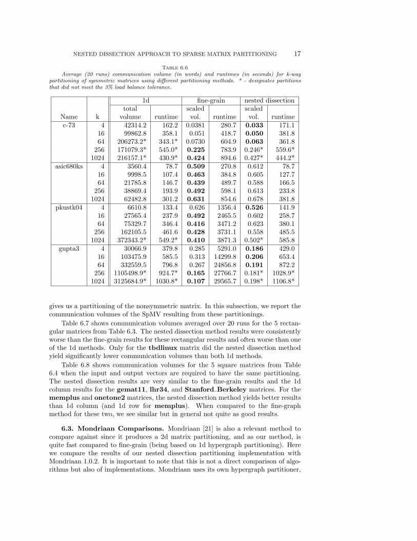
We partition the 4 larger symmetric matrices shown in Table 6.2 using 1d col-umn, fine-grain, and the nested dissection methods of partitioning for 4, 16, 64, 256,and 1024 parts. These matrices were chosen to demonstrate instances in which 1dpartitioning is insufficient. We picked these examples based on a comparison of the1d and fine-grain partitioning methods. The resulting communication volumes for thepartitioning of these matrices is shown in Table 6.6. As expected, our nested dissec-tion method performs much better than 1d (scaled volumes significantly less than 1).When compared to the fine-graph method, we see similar but in general not quite asgood results. Again, we see a great improvement over fine-grain in terms of runtime(up to 96% decrease in the runtime).

6.2. Nonsymmetric Matrices. We partitioned the 10 nonsymmetric matricesshown in Tables 6.3 and 6.4 using 1d column, 1d row, fine-grain, and the nesteddissection methods of partitioning for 4, 16, 64, and 256 parts. However, in order touse the nested dissection partition method with the nonsymmetric matrices, we haveto form bipartite graphs as described in Section 5. We can then apply the nesteddissection implementation outlined in Section 4 to partition the bipartite graph, which


Table 6.6Average (20 runs) communication volume (in words) and runtimes (in seconds) for k-way

partitioning of symmetric matrices using different partitioning methods. * - designates partitionsthat did not meet the 3% load balance tolerance.

1d fine-grain nested dissectiontotal scaled scaled

Name k volume runtime vol. runtime vol. runtimec-73 4 42314.2 162.2 0.0381 280.7 0.033 171.1

16 99862.8 358.1 0.051 418.7 0.050 381.864 206273.2* 343.1* 0.0730 604.9 0.063 361.8

256 171079.3* 545.0* 0.225 783.9 0.246* 559.6*1024 216157.1* 430.9* 0.424 894.6 0.427* 444.2*

asic680ks 4 3560.4 78.7 0.509 270.8 0.612 78.716 9998.5 107.4 0.463 384.8 0.605 127.764 21785.8 146.7 0.439 489.7 0.588 166.5

256 38869.4 193.9 0.492 598.1 0.613 233.81024 62482.8 301.2 0.631 854.6 0.678 381.8

pkustk04 4 6610.8 133.4 0.626 1356.4 0.526 141.916 27565.4 237.9 0.492 2465.5 0.602 258.764 75329.7 346.4 0.416 3471.2 0.623 380.1

256 162105.5 461.6 0.428 3731.1 0.558 485.51024 372343.2* 549.2* 0.410 3871.3 0.502* 585.8

gupta3 4 30066.9 379.8 0.285 5291.0 0.186 429.016 103475.9 585.5 0.313 14299.8 0.206 653.464 332559.5 796.8 0.267 24856.8 0.191 872.2

256 1105498.9* 924.7* 0.165 27766.7 0.181* 1028.9*1024 3125684.9* 1030.8* 0.107 29565.7 0.198* 1106.8*

gives us a partitioning of the nonsymmetric matrix. In this subsection, we report thecommunication volumes of the SpMV resulting from these partitionings.

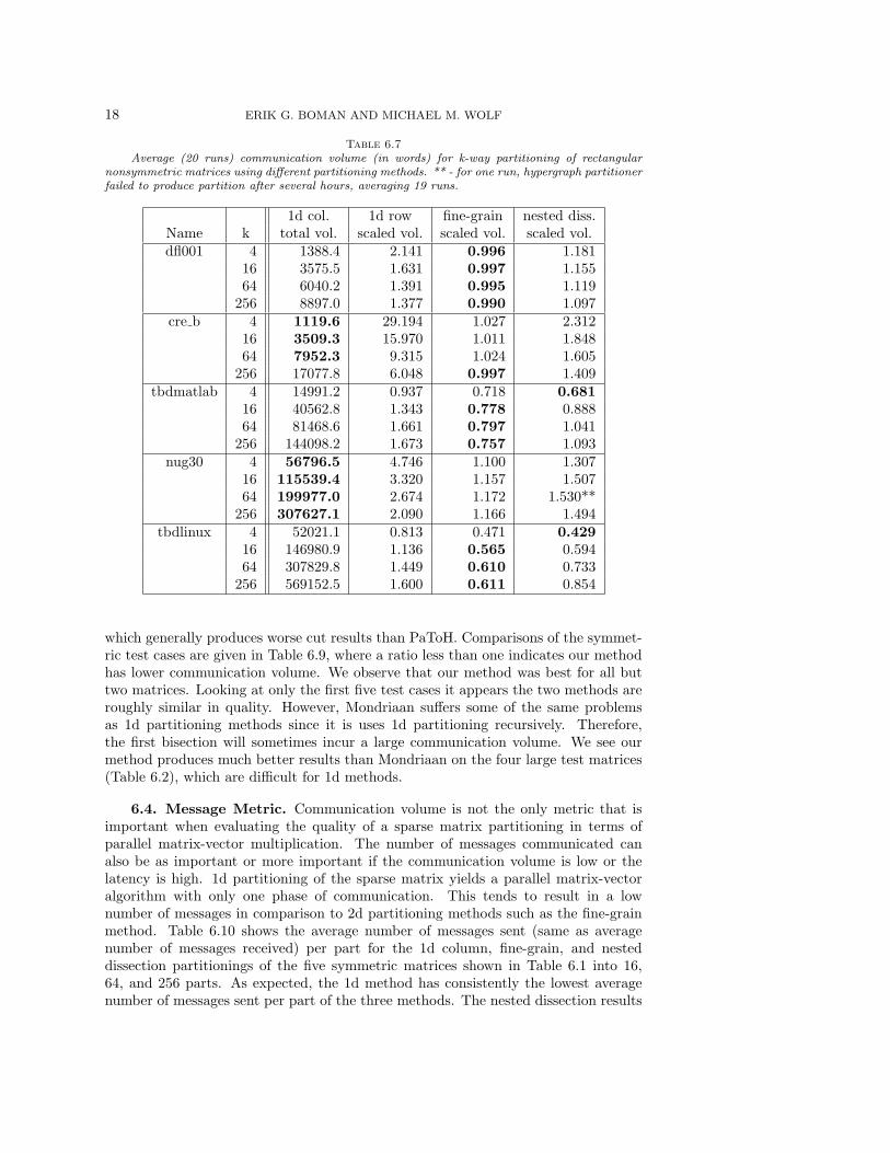
Table 6.7 shows communication volumes averaged over 20 runs for the 5 rectan-gular matrices from Table 6.3. The nested dissection method results were consistentlyworse than the fine-grain results for these rectangular results and often worse than oneof the 1d methods. Only for the tbdlinux matrix did the nested dissection methodyield significantly lower communication volumes than both 1d methods.

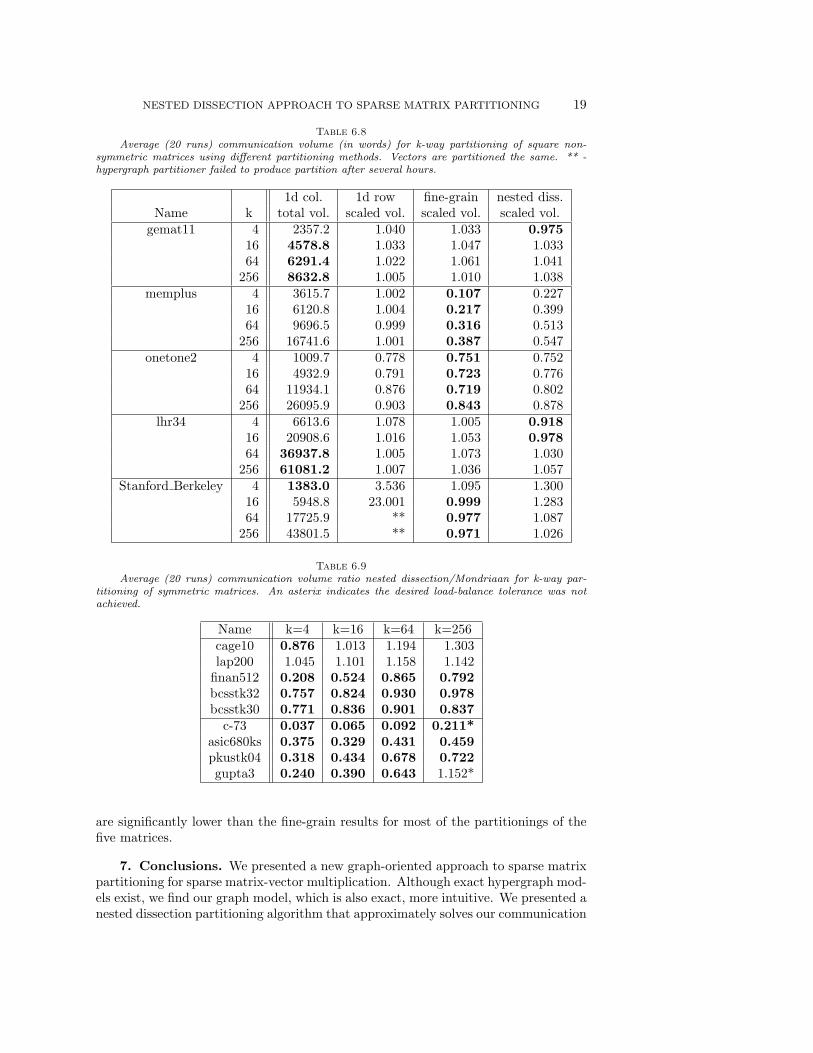
Table 6.8 shows communication volumes for the 5 square matrices from Table6.4 when the input and output vectors are required to have the same partitioning.The nested dissection results are very similar to the fine-grain results and the 1dcolumn results for the gemat11, lhr34, and Stanford Berkeley matrices. For thememplus and onetone2 matrices, the nested dissection method yields better resultsthan 1d column (and 1d row for memplus). When compared to the fine-graphmethod for these two, we see similar but in general not quite as good results.

6.3. Mondriaan Comparisons. Mondriaan [21] is also a relevant method tocompare against since it produces a 2d matrix partitioning, and as our method, isquite fast compared to fine-grain (being based on 1d hypergraph partitioning). Herewe compare the results of our nested dissection partitioning implementation withMondriaan 1.0.2. It is important to note that this is not a direct comparison of algo-rithms but also of implementations. Mondriaan uses its own hypergraph partitioner,


Table 6.7Average (20 runs) communication volume (in words) for k-way partitioning of rectangular

nonsymmetric matrices using different partitioning methods. ** - for one run, hypergraph partitionerfailed to produce partition after several hours, averaging 19 runs.

1d col. 1d row fine-grain nested diss.Name k total vol. scaled vol. scaled vol. scaled vol.dfl001 4 1388.4 2.141 0.996 1.181

16 3575.5 1.631 0.997 1.15564 6040.2 1.391 0.995 1.119

256 8897.0 1.377 0.990 1.097cre b 4 1119.6 29.194 1.027 2.312

16 3509.3 15.970 1.011 1.84864 7952.3 9.315 1.024 1.605

256 17077.8 6.048 0.997 1.409tbdmatlab 4 14991.2 0.937 0.718 0.681

16 40562.8 1.343 0.778 0.88864 81468.6 1.661 0.797 1.041

256 144098.2 1.673 0.757 1.093nug30 4 56796.5 4.746 1.100 1.307

16 115539.4 3.320 1.157 1.50764 199977.0 2.674 1.172 1.530**

256 307627.1 2.090 1.166 1.494tbdlinux 4 52021.1 0.813 0.471 0.429

16 146980.9 1.136 0.565 0.59464 307829.8 1.449 0.610 0.733

256 569152.5 1.600 0.611 0.854

which generally produces worse cut results than PaToH. Comparisons of the symmet-ric test cases are given in Table 6.9, where a ratio less than one indicates our methodhas lower communication volume. We observe that our method was best for all buttwo matrices. Looking at only the first five test cases it appears the two methods areroughly similar in quality. However, Mondriaan suffers some of the same problemsas 1d partitioning methods since it is uses 1d partitioning recursively. Therefore,the first bisection will sometimes incur a large communication volume. We see ourmethod produces much better results than Mondriaan on the four large test matrices(Table 6.2), which are difficult for 1d methods.

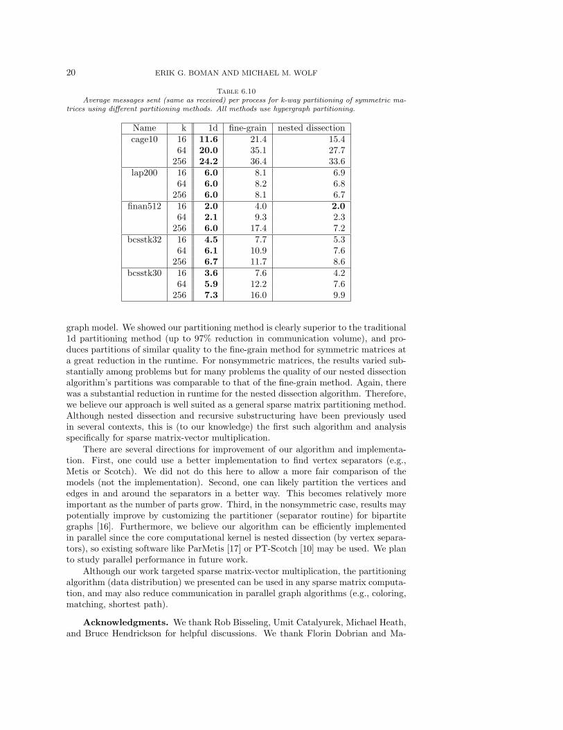
6.4. Message Metric. Communication volume is not the only metric that isimportant when evaluating the quality of a sparse matrix partitioning in terms ofparallel matrix-vector multiplication. The number of messages communicated canalso be as important or more important if the communication volume is low or thelatency is high. 1d partitioning of the sparse matrix yields a parallel matrix-vectoralgorithm with only one phase of communication. This tends to result in a lownumber of messages in comparison to 2d partitioning methods such as the fine-grainmethod. Table 6.10 shows the average number of messages sent (same as averagenumber of messages received) per part for the 1d column, fine-grain, and nesteddissection partitionings of the five symmetric matrices shown in Table 6.1 into 16,64, and 256 parts. As expected, the 1d method has consistently the lowest averagenumber of messages sent per part of the three methods. The nested dissection results


Table 6.8Average (20 runs) communication volume (in words) for k-way partitioning of square non-

symmetric matrices using different partitioning methods. Vectors are partitioned the same. ** -hypergraph partitioner failed to produce partition after several hours.

1d col. 1d row fine-grain nested diss.Name k total vol. scaled vol. scaled vol. scaled vol.

gemat11 4 2357.2 1.040 1.033 0.97516 4578.8 1.033 1.047 1.03364 6291.4 1.022 1.061 1.041

256 8632.8 1.005 1.010 1.038memplus 4 3615.7 1.002 0.107 0.227

16 6120.8 1.004 0.217 0.39964 9696.5 0.999 0.316 0.513

256 16741.6 1.001 0.387 0.547onetone2 4 1009.7 0.778 0.751 0.752

16 4932.9 0.791 0.723 0.77664 11934.1 0.876 0.719 0.802

256 26095.9 0.903 0.843 0.878lhr34 4 6613.6 1.078 1.005 0.918

16 20908.6 1.016 1.053 0.97864 36937.8 1.005 1.073 1.030

256 61081.2 1.007 1.036 1.057Stanford Berkeley 4 1383.0 3.536 1.095 1.300

16 5948.8 23.001 0.999 1.28364 17725.9 ** 0.977 1.087

256 43801.5 ** 0.971 1.026

Table 6.9Average (20 runs) communication volume ratio nested dissection/Mondriaan for k-way par-

titioning of symmetric matrices. An asterix indicates the desired load-balance tolerance was notachieved.

Name k=4 k=16 k=64 k=256cage10 0.876 1.013 1.194 1.303lap200 1.045 1.101 1.158 1.142

finan512 0.208 0.524 0.865 0.792bcsstk32 0.757 0.824 0.930 0.978bcsstk30 0.771 0.836 0.901 0.837

c-73 0.037 0.065 0.092 0.211*asic680ks 0.375 0.329 0.431 0.459pkustk04 0.318 0.434 0.678 0.722gupta3 0.240 0.390 0.643 1.152*

are significantly lower than the fine-grain results for most of the partitionings of thefive matrices.

7. Conclusions. We presented a new graph-oriented approach to sparse matrixpartitioning for sparse matrix-vector multiplication. Although exact hypergraph mod-els exist, we find our graph model, which is also exact, more intuitive. We presented anested dissection partitioning algorithm that approximately solves our communication


Table 6.10Average messages sent (same as received) per process for k-way partitioning of symmetric ma-

trices using different partitioning methods. All methods use hypergraph partitioning.

Name k 1d fine-grain nested dissectioncage10 16 11.6 21.4 15.4

64 20.0 35.1 27.7256 24.2 36.4 33.6

lap200 16 6.0 8.1 6.964 6.0 8.2 6.8

256 6.0 8.1 6.7finan512 16 2.0 4.0 2.0

64 2.1 9.3 2.3256 6.0 17.4 7.2

bcsstk32 16 4.5 7.7 5.364 6.1 10.9 7.6

256 6.7 11.7 8.6bcsstk30 16 3.6 7.6 4.2

64 5.9 12.2 7.6256 7.3 16.0 9.9

graph model. We showed our partitioning method is clearly superior to the traditional1d partitioning method (up to 97% reduction in communication volume), and pro-duces partitions of similar quality to the fine-grain method for symmetric matrices ata great reduction in the runtime. For nonsymmetric matrices, the results varied sub-stantially among problems but for many problems the quality of our nested dissectionalgorithm’s partitions was comparable to that of the fine-grain method. Again, therewas a substantial reduction in runtime for the nested dissection algorithm. Therefore,we believe our approach is well suited as a general sparse matrix partitioning method.Although nested dissection and recursive substructuring have been previously usedin several contexts, this is (to our knowledge) the first such algorithm and analysisspecifically for sparse matrix-vector multiplication.

There are several directions for improvement of our algorithm and implementa-tion. First, one could use a better implementation to find vertex separators (e.g.,Metis or Scotch). We did not do this here to allow a more fair comparison of themodels (not the implementation). Second, one can likely partition the vertices andedges in and around the separators in a better way. This becomes relatively moreimportant as the number of parts grow. Third, in the nonsymmetric case, results maypotentially improve by customizing the partitioner (separator routine) for bipartitegraphs [16]. Furthermore, we believe our algorithm can be efficiently implementedin parallel since the core computational kernel is nested dissection (by vertex separa-tors), so existing software like ParMetis [17] or PT-Scotch [10] may be used. We planto study parallel performance in future work.

Although our work targeted sparse matrix-vector multiplication, the partitioningalgorithm (data distribution) we presented can be used in any sparse matrix computa-tion, and may also reduce communication in parallel graph algorithms (e.g., coloring,matching, shortest path).

Acknowledgments. We thank Rob Bisseling, Umit Catalyurek, Michael Heath,and Bruce Hendrickson for helpful discussions. We thank Florin Dobrian and Ma-


hantesh Halappanavar for providing a matching code used to produce vertex separa-tors. This work was funded by the US Dept. of Energy’s Office of Science throughthe CSCAPES Institute and the SciDAC program.

REFERENCES

[1] C. Aykanat, A. Pinar, and U. V. Catalyurek. Permuting sparse rectangular matrices intoblock-diagonal form. SIAM Journal on Scientific Computing, 25(6):1860–1879, 2004.

[2] C. Berge. Graphs and Hypergraphs, volume 6 of North-Holland Mathematical Library. ElsevierScience Publishing Company, 1973.

[3] C. Berge. Hypergraphs: Combinatorics of Finite Sets, volume 45 of North-Holland Mathemat-ical Library. Elsevier Science Publishing Company, 1989.

[4] R. H. Bisseling. Parallel Scientific Computing: A structured approach using BSP and MPI.Oxford University Press, 2004.

[5] R. H. Bisseling and W. Meesen. Communication balancing in parallel sparse matrix-vectormultiplication. Electronic Transactions on Numerical Analysis, 21:47–65, 2005.

[6] E. G. Boman. A nested dissection approach to sparse matrix partitioning. In Proc. AppliedMath. and Mechanics, volume 7, 2007. Presented at ICIAM07, Zurich, Switzerland, July2007.

[7] U. Catalyurek and C. Aykanat. Hypergraph-partitioning-based decomposition for parallelsparse-matrix vector multiplication. IEEE Trans. Parallel Dist. Systems, 10(7):673–693,1999.

[8] U. Catalyurek and C. Aykanat. A fine-grain hypergraph model for 2d decomposition of sparsematrices. In Proc. IPDPS 8th Int’l Workshop on Solving Irregularly Structured Problemsin Parallel (Irregular 2001), April 2001.

[9] U. Catalyurek and C. Aykanat. A hypergraph-partitioning approach for coarse-grain decompo-sition. In Proc. Supercomputing 2001. ACM, 2001.

[10] C. Chevalier and F. Pellegrini. PT-SCOTCH: A tool for efficient parallel graph ordering. ParallelComputing, 34(6–8):318–331, Jul. 2007.

[11] T. A. Davis. The University of Florida Sparse Matrix Collection, 1994. Matrices found athttp://www.cise.ufl.edu/research/sparse/matrices/.

[12] K. Devine, E. Boman, R. Heaphy, B. Hendrickson, and C. Vaughan. Zoltan data managementservices for parallel dynamic applications. Computing in Science and Engineering, 4(2):90–97, 2002.

[13] A. George. Nested dissection of a regular finite-element mesh. SIAM Journal on NumericalAnalysis, 10:345–363, 1973.

[14] A. George, M. T. Heath, J. W.-H. Liu, and E. G.-Y. Ng. Solution of sparse positive definitesystems on a hypercube. Journal of Computational and Applied Mathematics, 27:129–156, 1989. Also available as Technical Report ORNL/TM-10865, Oak Ridge NationalLaboratory, Oak Ridge, TN, 1988.

[15] A. George, J. W.-H. Liu, and E. G.-Y. Ng. Communication results for parallel sparse Choleskyfactorization on a hypercube. Parallel Computing, 10(3):287–298, May 1989.

[16] B. Hendrickson and T. G. Kolda. Partitioning rectangular and structurally nonsymmetric sparsematrices for parallel computation. SIAM Journal on Scientific Computing, 21(6):2048–2072, 2000.

[17] G. Karypis and V. Kumar. Parmetis: Parallel graph partitioning and sparse matrix orderinglibrary. Technical Report 97-060, Dept. Computer Science, University of Minnesota, 1997.http://www.cs.umn.edu/~metis.

[18] G. Karypis and V. Kumar. METIS 4.0: Unstructured graph partitioning and sparse matrixordering system. Technical report, Dept. Computer Science, University of Minnesota, 1998.http://www.cs.umn.edu/˜metis.

[19] R. J. Lipton, D. J. Rose, and R. E. Tarjan. Generalized nested dissection. SIAM Journal onNumerical Ananlysis, 16:346–358, 1979.

[20] A. Trifunovic and W. J. Knottenbelt. A general graph model for representing exact communica-tion volume in parallel sparse matrix-vector multiplication. In Proc. of 21st InternationalSymposium on Computer and Information Sciences (ISCIS 2006), pages 813–824, 2006.

[21] B. Vastenhouw and R. H. Bisseling. A two-dimensional data distribution method for parallelsparse matrix-vector multiplication. SIAM Review, 47(1):67–95, 2005.

Documents

A Nested Dissection Approach to Sparse Matrix Partitioning ...egboman/papers/ND-SISC.pdf · A NESTED DISSECTION APPROACH TO SPARSE MATRIX PARTITIONING FOR PARALLEL COMPUTATIONS