Eur. Phys. J. D (2020) 74: 115https://doi.org/10.1140/epjd/e2020-10069-8 THE EUROPEAN

PHYSICAL JOURNAL DRegular Article

A network of superconducting gravimeters as a detectorof matter with feeble nongravitational coupling?

Wenxiang Hu1, Matthew M. Lawson2,3, Dmitry Budker4,5, Nataniel L. Figueroa4,a, Derek F. Jackson Kimball6,Allen P. Mills Jr.7, and Christian Voigt8

1 School of Physics, Peking University, Beijing, P.R. China2 The Oskar Klein Centre for Cosmoparticle Physics, Department of Physics, Stockholm University, AlbaNova,

Stockholm 10691, Sweden3 Nordita, KTH Royal Institute of Technology and Stockholm University, Roslagstullbacken 23, Stockholm 10691, Sweden4 Helmholtz Institut, Johannes Gutenberg-Universitat Mainz, Mainz 55128, Germany5 Department of Physics, University of California, Berkeley, CA 94720, USA6 Department of Physics, California State University – East Bay, Hayward, CA, USA7 Department of Physics and Astronomy, University of California, Riverside, CA, USA8 GFZ German Research Centre for Geosciences, Telegrafenberg, Potsdam, Germany

Received 5 February 2020 / Received in final form 31 March 2020Published online 11 June 2020

c© The Author(s) 2020. This article is published with open access at Springerlink.com

Abstract. Hidden matter that interacts only gravitationally would oscillate at characteristic frequencieswhen trapped inside of Earth. For small oscillations near the center of the Earth, these frequencies arearound 300µHz. Additionally, signatures at higher harmonics would appear because of the non-uniformityof Earth’s density. In this work, we use data from a global network of gravimeters of the InternationalGeodynamics and Earth Tide Service (IGETS) to look for these hypothetical trapped objects. We find noevidence for such objects with masses on the order of 1014 kg or greater with an oscillation amplitude of0.1 re. It may be possible to improve the sensitivity of the search by several orders of magnitude via betterunderstanding of the terrestrial noise sources and more advanced data analysis.

1 Introduction

A classic result in Newtonian gravity is that if a small massis orbiting inside a large mass of uniform density, such thatthe orbit is entirely contained in the interior of the largemass, the period of the orbit is fixed by the density of thelarge mass, and independent of the particulars of the orbit.This is because the system can be described as a three-dimensional harmonic oscillator. In the case of a massinside a sphere with uniform density equal to the aver-age density of the Earth, the period of such orbits wouldbe approximately 80 min. Such a scenario is impossiblewith masses comprised of ordinary matter because of non-gravitational interactions. However, the situation could behypothetically realized if the small mass is comprised ofsome “hidden matter” (we call it a hidden internal object,HIO) that has only feeble, if any, non-gravitational inter-actions with normal matter. Furthermore, it is known thatsuch hidden matter exists: evidence from many indepen-

? Contribution to the Topical Issue “Quantum Technologiesfor Gravitational Physics”, edited by Tanja Mehlstaubler,Yanbei Chen, Guglielmo M. Tino and Hsien-Chi Yeh.

a e-mail: figueroa@uni-mainz.de

dent observations point to the existence of dark matter [1],an invisible substance which may interact with ordinarymatter primarily via gravity. If some fraction of this hid-den matter is gravitationally bound within the Earth, thishypothetical scenario of a hidden internal object could berealized.

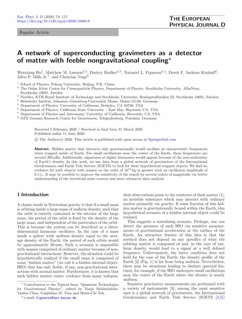
This suggests a tantalizing scenario. Perhaps, one candetect the presence of such HIO via sensitive measure-ments of gravitational acceleration at the surface of theEarth. An attractive feature of this idea is that themethod does not depend on any specifics of what theorbiting matter is composed of and, in the case of uni-form density, would lead to a signal at a well definedfrequency. Unfortunately, the latter condition does nothold for the case of the Earth: the density profile of theEarth [2] (Fig. 1) is far from being uniform. Nevertheless,there may be situations leading to distinct spectral fea-tures, for example, if the HIO undergoes small oscillationsnear the center of the Earth where the density is nearlyuniform.

Sensitive gravimetry measurements are performed witha variety of instruments [3]; among the most sensitiveones is a global network of gravimeters, the InternationalGeodynamics and Earth Tide Service (IGETS [4,5])

Page 2 of 10 Eur. Phys. J. D (2020) 74: 115

Fig. 1. The density profile of the Earth based on the Prelimi-nary Reference Earth model (PREM) [2]. re = 6371 km is themean radius of the Earth, ρ = 5.51 g cm−3 is the average den-sity of the Earth, and ρ0 = 13.1 g cm−3 is the density at theEarth’s center.

discussed in more detail in Section 4. If HIOs exist insidethe Earth, each gravimeter in the network would see aweak periodic signal at its characteristic frequencies, witha phase depending on the geometry of the orbit and loca-tion of the gravimeter. The presence of such frequencycomponents in a Fourier analysis of the gravimeter time-sequence data could indicate the presence of a HIO if itcan be adequately differentiated from naturally occurringspectral features. This methodology is similar to that usedby geophysicists to search for periodic oscillations of thesolid core of the Earth, the so-called Slichter mode [6,7].

There are also entirely different scenarios that can leadto signals in principle observable with gravimeters. Forexample, ultralight scalar dark-matter field can lead toeffective variation of fundamental constants, including themass of the baryons [8]. This would cause a sinusoidal vari-ation of the Earth mass at a frequency equal to the oscil-lation frequency of the dark-matter field. This could be,for example, the background galactic dark matter nomi-nally oscillating at the Compton frequency of the under-lying boson [8], an Earth-bound halo [9], or the field in a“boson star” encountering the Earth [10] and leading to atransient (rather than a persistent) signal. Some such sce-narios have been recently analyzed in reference [11]. Thedata from the gravimeter network were also used in ref-erence [12] to set limits on a possible violation of Lorentzinvariance.

In this paper, we survey the scenarios that could poten-tially lead to observable effects of the HIO, discuss thesensitivity of a gravimeter network, and present a prelim-inary analysis of a historical record of the IGETS data.Finally, we assess the prospects of the future HIO searchesbased on these techniques.

During the preparation of this manuscript, we becameaware of a similar work [13]. While the basic idea andapproach of reference [13] are close to ours, the specificsare different and complementary.

2 Capture/formation scenarios and theirdifficulties

One can imagine a few different scenarios in which an oscil-latory gravitational signal can be produced by hidden sec-tor objects gravitationally bound to the Earth. The moststudied in the literature (see e.g., [9,14]) is the formationof diffuse halos of dark matter particles around the Earth1.One could imagine a scenario in which a meteor impactor other violent jolt set up relative oscillations betweensuch a halo and Earth. However, numerical models of ahalo of non-interacting particles on orbits around a pointmass have shown that any overall coherent oscillationsof the halo would damp out on orbital time scales andbecome unobservable. This can be seen intuitively by not-ing that each particle in the halo has (generally) a differentorbital frequency, thus the overall oscillations will not addcoherently.

A second scenario is massive compact hidden-sectorobjects on orbits within, or possibly extending slightlybeyond, the surface of the Earth. As previously noted(and as will be quantified below), objects with such tra-jectories do not have the enticing property of single orbit-independent orbital frequencies, and thus are in generaldifficult to detect by the methods discussed in this paper.

The third scenario is massive compact objects on orbitsconfined sufficiently close to the center of the Earth wherethe Earth’s density is essentially uniform. It is such objectswhich we will principally consider. We thus define aHidden Internal Object (HIO) as a compact object thatorbits as a single object, entirely within the Earth’s core.

How could HIOs be formed? In general this is a difficultproblem for non/minimally interacting objects. An objectstarting far from the Earth following a trajectory that willbring it within the interior of the Earth starts with a grav-itational potential energy equal to the necessary energy toreach the Earth’s escape velocity. Moreover, the velocityof generic objects in the galaxy relative to the Earth isgenerally on the order of the Milky Way virial velocity of220 km s−1, whereas the escape velocity for the Earth is11 km s−1, so some strongly inelastic process is needed foreven orbital capture, and additional energy dissipation isrequired to localize the object to the inside of the Earth.Objects of interest to us might be expected, in general,to have nearly dissipationless interactions with ordinarymatter. However, this does not necessarily exclude dissi-pation due to self-interactions or interactions with otherforms of dark matter in the hidden sector. For example,one possible capture scenario is that a captured objectoriginates from a diffuse “cloud” in which a small partis sheared away and gets captured by the Earth in an

1 One model suggests that axion quark nuggets (AQN) [15]explain the similarity of the dark and visible cosmological matterdensities: in this model annihilation of anti-AQNs with visible mat-ter produces a terrestrial halo of axion dark matter when AQNs hitthe Earth. Although only a small fraction

(≈10−17

)of the emitted

particles stay bound, the accumulation of axions over the history ofthe Earth can still result in a halo (see [14] for a detailed discus-sions of the process), although in this scenario the halo is external,virial, and of order 0.1 kg and thus not suitable for detection withgravimeters.

Eur. Phys. J. D (2020) 74: 115 Page 3 of 10

effective “three-body” collision. Such scenarios are notuncommon in celestial dynamics, where gravitational tidalforces can rip apart bound objects and capture mate-rial [16]. The self-interaction scenario, however, has twoserious problems. One is that it requires the hidden-sectorobject to be only weakly self-bound so that some of thematerial can be gravitationally sheared off, but this typeof weak self interaction will generically lead to either theformation of rings of the material (making our detectionscheme unworkable) or to complete virialization (with thesame effect). Additionally this scenario requires the mat-ter being captured to have non-trivial self-interactions,which are generically constrained by galaxy cluster merg-ers [17].

A further difficulty is that even if a dense object is cap-tured into an Earth orbit, only extremely eccentric orbits(those intersecting the Earth) plus a dissipative interac-tion between the compact object and the Earth offers aplausible method for confining the object to the interior ofEarth. But, such an interaction would damp the orbit untilthe object is confined to be mostly stationary at the cen-ter of the Earth. A possible alternative energy-loss mech-anism related to gravitational polarization of the Earth isdiscussed in Appendix B.

We also note that regardless of capture mechanism, anydamping mechanism which is enhanced for large velocitiesand suppressed for small velocities will tend to producecircular orbits.

We emphasize that a specific consistent scenario for HIOformation is yet to be worked out.

To give a sense of scale to our discussions of HIO masses,we consider several quantities. The total amount of darkmatter enclosed in a sphere with a radius equal to thatof the solar system (under the assumptions of the stan-dard halo model and assuming uniform density of thedark matter) is ≈3 × 1017 kg, while that contained in asphere with the radius of the Earth is on the order of 1 kg.Another interesting mass to compare is obtained by con-sidering the volume V traced out through the galaxy bythe Earth as it has travelled through space since its for-mation: V = vAT ≈ 1036 m3, where v ≈ 2 × 105 m/sis the speed of the Earth relative to the galactic restframe, A ≈ 1014 m2 is the Earth’s cross-sectional area,and T ≈ 4.5 × 109 years is the age of the Earth. Mul-tiplying V by the average dark matter density ρDM ≈0.4 GeV/c2/cm3 ≈ 7×10−22 kg/m3 (here c is the speed oflight), we get that the total dark matter mass the Earthhas passed through is about: M ∼ 1015 kg. The feebleinteractions between dark matter and baryonic mattermakes this quantity of dark matter unachievable in nor-mal capture scenarios but it can serve as an upper limiton dark matter capture.

3 Detection signatures

As mentioned above, the non-uniformity of the Earth’sdensity leads to broadening in the spectrum of the HIOorbital frequencies, nominally removing the attractive fea-ture of the original idea that one may just look for orbitsat a single unique and predictable frequency.

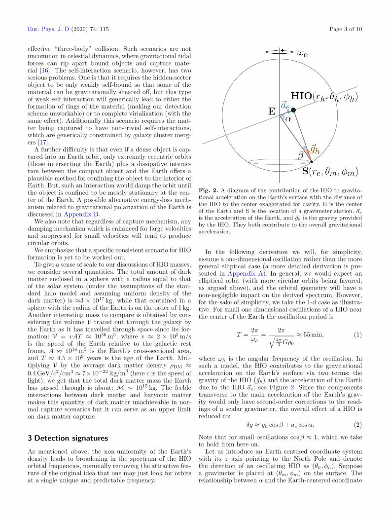
Fig. 2. A diagram of the contribution of the HIO to gravita-tional acceleration on the Earth’s surface with the distance ofthe HIO to the center exaggerated for clarity. E is the centerof the Earth and S is the location of a gravimeter station. ~ae

is the acceleration of the Earth, and ~gh is the gravity providedby the HIO. They both contribute to the overall gravitationalacceleration.

In the following derivation we will, for simplicity,assume a one-dimensional oscillation rather than the moregeneral elliptical case (a more detailed derivation is pre-sented in Appendix A). In general, we would expect anelliptical orbit (with more circular orbits being favored,as argued above), and the orbital geometry will have anon-negligible impact on the derived spectrum. However,for the sake of simplicity, we take the 1-d case as illustra-tive. For small one-dimensional oscillations of a HIO nearthe center of the Earth the oscillation period is

T =2πωh

=2π√

4π3 Gρ0

≈ 55 min, (1)

where ωh is the angular frequency of the oscillation. Insuch a model, the HIO contributes to the gravitationalacceleration on the Earth’s surface via two terms: thegravity of the HIO (~gh) and the acceleration of the Earthdue to the HIO ~ae; see Figure 2. Since the componentstransverse to the main acceleration of the Earth’s grav-ity would only have second-order corrections to the read-ings of a scalar gravimeter, the overall effect of a HIO isreduced to:

δg ≈ gh cosβ + ae cosα. (2)

Note that for small oscillations cosβ ≈ 1, which we taketo hold from here on.

Let us introduce an Earth-centered coordinate systemwith its z axis pointing to the North Pole and denotethe direction of an oscillating HIO as (θh, φh). Supposea gravimeter is placed at (θm, φm) on the surface. Therelationship between α and the Earth-centered coordinate

Page 4 of 10 Eur. Phys. J. D (2020) 74: 115

system is:

cosα = sin θh sin θm cos (ω0t+ φm − φh) + cos θh cos θm,(3)

where ω0 is the the angular frequency of the rotation ofthe Earth. Thus, the gravitational acceleration due to theHIO would contribute to the gravimeter signal as:

δg =Gmh

r2e

+(

2 +ρ0

ρ

)Gmh

r3e

Ah

[sin θh sin θm cos

(ω0t

+ φm − φh)

+ cos θh cos θm]

cosωht, (4)

where mh and Ah are the mass and amplitude of the HIOoscillation, ρ = 5.5 g cm−3 is the average density of theEarth, and ρ0 = 13.1 g cm−3 is the density of the Earth’score. In this scenario, the HIO acts as a harmonic oscil-lator with a specific frequency, and the frequency is splitbecause of the rotation of the Earth. Note however thatwhile this splitting is exactly the sidereal frequency of theEarth’s rotation in the simplified case of a 1-d non-co-rotating oscillation considered here, in general it woulddepend strongly on the orbital geometry (and for cer-tain orbits be zero, e.g., a circular equatorial orbit). Dueto the non-uniformity of the Earth density (see Fig. 1),this spectral pattern holds for oscillations not exceed-ing ≈0.1 re in amplitude. Note that the second term inequation (4) is smaller than the first term by roughly anorder of γ =

(2 + ρ0

ρ

)Ah

re, so assuming that Ah ≈ 0.1 re,

γ ≈ 0.4.If the amplitude of such oscillation is large, there will

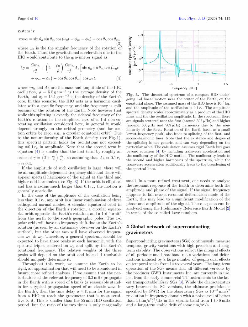
be an amplitude-dependent frequency shift and there willappear spectral harmonics of the signal at the third andhigher odd harmonics (see Fig. 3). If the orbit is ellipticaland has a radius much larger than 0.1 re, the motion isgenerally aperiodic.

In the case of the amplitude of the oscillation beingless than 0.1 re, any orbit is a linear combination of threeorthogonal normal modes. A circular equatorial orbit inthe direction of the Earth’s rotation, a circular equato-rial orbit opposite the Earth’s rotation, and a 1-d “orbit”from the north to the south geographic poles. The 1-dpolar orbit will have no frequency shift due to the Earth’srotation (as seen by an stationary observer on the Earth’ssurface), but the other two will have observed frequen-cies ωh ± ω0. Therefore, a general spectrum should beexpected to have three peaks at each harmonic, with thespectral triplet centered on ωh and split by the Earth’srotational frequency. The relative weights of the threepeaks will depend on the orbit and indeed if resolvableshould uniquely determine it.

Throughout this work, we assume the Earth to berigid, an approximation that will need to be abandoned infuture, more refined analyses. If we assume that the per-turbations at the relevant frequency of 0.3 mHz propagatein the Earth with a speed of 6 km/s (a reasonable stand-in for a typical propagation speed of an elastic wave inthe Earth), then the time delay is ≈15 min for the signalfrom a HIO to reach the gravimeter that is most sensi-tive to it. This is smaller than the 55 min HIO oscillationperiod, but the ratio of the two times is only marginally

Fig. 3. The theoretical spectrum of a compact HIO under-going 1-d linear motion near the center of the Earth, on theequatorial plane. The assumed mass of the HIO here is 1013 kg,and the amplitude of the oscillation is 0.1 re. The amplitudespectral density scales approximately as a product of the HIOmass and the the oscillation amplitude. In the spectrum, thereare signals centered near the first (around 303µHz) and higher(around 606µHz and 909µHz) harmonics due to the non-linearity of the force. Rotation of the Earth (seen as a smalllowest-frequency peak) also leads to splitting of the first- andsecond-harmonic lines. Note that the existence and degree ofthe splitting is not generic, and can vary depending on theparticular orbit. The calculation assumes rigid Earth but goesbeyond equation (4) by including transverse acceleration andthe nonlinearity of the HIO motion. The nonlinearity leads tothe second and higher harmonics of the spectrum, while thetransverse acceleration additionally leads to the broadening ofthe spectral lines.

small. In a more refined treatment, one needs to analyzethe resonant response of the Earth to determine both theamplitude and phase of the signal. If the signal frequencyhappens to fall near a resonant deformation mode of theEarth, this may lead to a significant modification of thephase and amplitude of the signal. These aspects can beanalysed using the Preliminary Reference Earth Model [2]in terms of the so-called Love numbers.

4 Global network of superconductinggravimeters

Superconducting gravimeters (SGs) continuously measuretemporal gravity variations with high precision and long-term stability. The observations reflect the integral effectsof all periodic and broadband mass variations and defor-mations induced by a large number of geophysical effectson temporal scales from 1 s to several years. The long-termoperation of the SGs means that all different versions bythe producer GWR Instruments Inc. are currently in use,i.e., from the early commercial TT instruments to the lat-est transportable iGrav SGs [3]. While the characteristicsvary between the SG versions, the ultimate precision isspecified by GWR for the observatory SGs as 10−3 nm/s2

resolution in frequency domain with a noise level of betterthan 1 (nm/s2)2/Hz in the seismic band from 1 to 8 mHzand a long-term stable drift of some nm/s2/a.

Eur. Phys. J. D (2020) 74: 115 Page 5 of 10

SG data sets are available from the database ofthe International Geodynamics and Earth Tides Service(IGETS) hosted by the Information System and DataCenter at GFZ [5]. Originating as Global GeodynamicsProject from 1997 to 2015 [18], since 2015 IGETS pro-vides freely accessible data from an increasing number ofstations and sensors all over the world (currently 42 and60, respectively) to support global geodetic and geophys-ical studies. The IGETS database provides three levels ofdata sets from raw gravity and local atmospheric pres-sure observations sampled at 1 or 2 s (level 1) to datasets corrected for instrumental perturbations (level 2) togravity residuals after particular geophysical corrections(level 3). Level 3 products are available for 26 stations and36 sensors processed by EOST Strasbourg at 1 min sam-pling [19]. These originate from specially processed level 2products at EOST and are reduced by gravity effects fromsolid Earth and ocean tides, atmospheric loading, polarmotion and length-of-day variations as well as instrumen-tal drift.

The specified SG precision of 10−3 nm/s2 offers greatpossibilities in combination with stacking methods usinggravity data sets from multiple stations of the IGETSnetwork [6]. Theoretically, the sensitivity for the detec-tion of small periodic signals could be enhanced by

√lmn

assuming coherent signals with the precision increase l formonthly averages as well as the total number of stations mand months n. However, in reality, the instrumental noisefrom the SGs is not only superseded by station noise [20]but, above all, by a complex and significant uncertaintybudget at the nm/s2 level from the modelling of mass re-distributions in the atmosphere, the oceans, and hydrol-ogy on a wide range of time scales [21]. In addition, allSG data sets are affected by free oscillations of the Earthexcited by large earthquakes in the target frequency rangeof 0.3 mHz in this study [3].

The gravimeter precision discussed above, assumingthat the geophysical effects may eventually be fully sub-tracted and ignoring other sources of noise, providesgrounds for optimistic estimates of what one might hopeto ultimately achieve in a search for HIO. For example,with a network with a similar number of stations as theexisting one and assuming signals from the stations areadded coherently and with on the order of a month ofaveraging time, the cumulative sensitivity could, in prin-ciple, reach on the order of 10−7 nm/s2. Taking an averageoscillation amplitude of Ah = 0.1 re (≈637 km), the small-est detectable mass of the network would be:

mmin =(

2 +ρ0

ρ

)−1δgr3

e

GAh= 1× 108 kg. (5)

This mass can be compared to the reference values dis-cussed at the end of Section 2.

5 Analysis and preliminary results

The essence of the data processing is as follows. Ouranalysis technique involves partitioning the time-domaingravity residuals from each station into one-month long

Fig. 4. (a) The amplitude spectral density of the IGETS level 3data sets, with baseline removal performed after the averaging.The large spike around 800µHz is due to the 0S0 “breathing”mode of Earth [2,22,23]. The inset (b) shows details around303µHz, where the signal from a HIO orbiting near the cen-ter of the Earth would lie. The dark red line corresponds tothe data with the minimum-detectable signal (m = 1014 kg)injected into it.

segments. We then perform a discrete Fourier trans-form, normalize by the sampling frequency and the exactsegment length, then take the magnitude squared. Theresulting quantity is known in the signal-processing lit-erature as a periodogram, which is an estimate of thepower spectral density. To improve this estimate, weaverage all the month-long periodograms from all sta-tions together to produce a single estimate of the truepower-spectral density (a process known as Bartlett’smethod). We take the square root to obtain the ampli-tude spectral density, then remove any overall baselineby fitting and then subtracting out a function of theform:

y(f) =A

f+B

f2+C

f3+D

f4+ y0. (6)

We only fit in the region of higher frequency than tidaleffects (>36.55µHz), to avoid tide-induced fit artifacts.This results in a single averaged spectrum; see Fig. 4a).Some of the spectral features seen in the spectrum arewell-known in geophysics. For example, the sharp spikearound 800µHz is the fundamental radial mode 0S0 [22].Other modes in the region of interest have been reported(see e.g., Fig. 21 and the corresponding discussion ofthe mode identification in Ref. [3]). There are also fea-tures in the data that do not generally appear in theraw gravity data from superconducting gravimeters andare possibly artifacts from reduction models used toobtain the level 3 data. This will be subject of furtherinvestigation.

We looked for a HIO by fitting three Lorentzians, onecentered around 303µHz, and the others centered around303µHz± 11.6µHz (corresponding to a period of 1 day)to the data, and did not detect a signature above noiseconsistent with the HIO scenario we have presented. Toestimate the minimum detectable HIO mass oscillating

Page 6 of 10 Eur. Phys. J. D (2020) 74: 115

with an amplitude of 0.1 re, we injected a signal (from oursimulations presented in Fig. 3) into the data. With this,we determined that the minimum injected signal that isdetected corresponds to a HIO mass of ≈1014 kg at thisradius. Details of the analysis can be found in Appendix C.Note that this is not a traditional exclusion limit of a mass,but of a mass on a specific orbit.

This upper bound on the signal, assuming an oscillation637 km (≈0.1 re), would corresponds to an acceleration ofδg of

δg =(

2 +ρ0

ρ

)mGAhr3e

= 72 pm/s2. (7)

Although this upper bound on the mass oscillatingwith an amplitude of 0.1 re is relatively small (≈10−10

of Earth’s mass), the current sensitivity is still severalorders of magnitude short of the estimated sensitivity inequation (5). This difference arises from various factors.Although the contributions of the instrument drift andpressure are largely removed already, the employed data-fix techniques may introduce errors. Also, there are tidesand nontidal loading factors, rainfall and other hydrologi-cal factors, station disturbances, seismic factors, and othernatural and anthropological contributions to the overallacceleration. Tides generally produce clear, discrete linesin the spectra that are harmonics of the tidal frequency(period ≈ 12 h), which have little impact on the region ofinterest (period ≈ 55 min). As for the seismic influences,there are both persistent oscillations, which are a responseto other periodic driving forces, which can be roughly eval-uated by the Earth model and transient incidences (e.g.,earthquakes), which, along with other transient factors,can be removed by data selection. Data selection is alsoan effective technique for dealing with nontidal and hydro-logical loading factors which can have an effect of as bigas ≈1× 104 nm/s2 over a few days. These effects producenoise-like spectra, deteriorating the sensitivity of the net-work to HIO signals [3].

In the future stages of this work, one should be ableto enhance the precision substantially by performing aphase sensitive analysis. Furthermore, the phase informa-tion would enable us to approximately determine the spe-cific orbit of a HIO within the Earth, as the phases of agravimeter signal would depend on its location on Earth’ssurface.

The stated HIO-mass sensitivity of 108 kg is based onthe assumption that the signals of different stations arecompletely correlated, and neglects all noise sources otherthan those of the sensors. In our case where HIO moveas a single object inside the Earth, the signal obtained bydifferent stations are indeed correlated. However, if otherpossible scenarios are to be considered, then the correla-tion would be incomplete and the sensitivity would dete-riorate.

We note that correlation-analysis techniques are cur-rently employed by the existing sensor networks suchas LIGO/VIRGO [24] for the detection of gravitationalwaves, as well as by magnetometer (GNOME [25]) andclock (e.g., GPS.DM [26]) networks for the detection ofthe galactic dark matter.

6 Conclusions and outlook

We have analyzed various possible scenarios of hiddengravitationally bound objects that have weak or no inter-actions (other than gravitation) with normal matter, andhave discussed their possible influence on the total gravi-tational field measured at the surface of the Earth. Withdata sets from IGETS, we used Fourier analysis to searchfor characteristic spectral lines that could be an indicationof the existence of such objects. Although no evidence hasbeen found, we estimate that the smallest detectable massusing the current network could perhaps ultimately reachas low as ≈1× 108 kg. Such hidden gravitationally boundobjects could potentially be related to nonbaryonic darkmatter.

An alternative scenario to HIO trapped in the Earthis a change of the Earth’s gravitational field under theinfluence of some background bosonic field, for example,that due to dilatons. Serving as dark matter candidates,dilatons and other bosonic fields can have linear inter-actions with nucleons, changing their effective masses atthe Compton frequency associated with the mass. Underappropriate conditions, the mass of the Earth could oscil-late slightly at the particle Compton frequency [8]. Thesuperconducting gravimeter data considered in this noteare resampled to the once per minute cadence, so thesmallest frequency that can be detected is 1/120 Hz, cor-responding to a particle mass of 3.5×10−17 eV. The modi-fication of the Earth mass by the presence of an oscillatingfield φ = φ0 cosωφt is described by

meff =

(1 +

√~cφΛ1

)me, (8)

where me is the mass of the Earth, ωφ is the frequency ofthe oscillating field, and φ0 = ~

√2ρDM/ (mφc) is related

to the mass of the bosonic particle mφ and the local den-sity of dark matter ρDM. Λ1 is the coupling constant aver-aged over all the Earth’s atoms.

Assuming the optimistic sensitivity of 10−17 g ≈10−7 nm/s2 discussed in Section 4, the network can detectsuch variance if

mφc2Λ1 ≤ 2.5× 1014 eV2, (9)

which is compatible to the sensitivity of future atominterferometers discussed in reference [8] and performingbetter than current equivalence-principle tests if mφ ≤1× 10−18 eV. Additionally, periodic mass variations ofEarth’s mass could appear as sidebands in Earth’s vibra-tional modes.

Another possibility is that there could be “boson stars”encountering the Earth that affect the gravitation field.Supposing such influence is only detectable when thedistance between the star and the Earth is closer than10 re and taking the characteristic relative velocity of theEarth and the boson star as the galactic virial velocity≈10−3 c, such transient signal would possibly last ≈5 min,which means that its timing is ideal for detection usingIGETS’s level-2 and level-3 data sets. According to anestimate in [10], the maximum acceleration felt during an

Eur. Phys. J. D (2020) 74: 115 Page 7 of 10

encounter is 10−19 g, so a significant improvement in sen-sitivity would be needed if one is to detect such eventsusing gravimeters.

In conclusion, advanced gravimeter networks could beuseful for detection of exotic matter and future improve-ments in the hardware and, particularly, in advanced dataanalysis may enable mounting competitive searches.

Open access funding provided by Projekt DEAL. The authorsacknowledge helpful discussions with Joshua Eby, Ernst M.Rasel, Surjeet Rajendran, and the members of the CASPErand GNOME collaborations. This work was supported in partby the European Research Council (ERC) under the EuropeanUnion Horizon 2020 research and innovation program (grantagreement No. 695405) and by the DFG via the ReinhartKoselleck project and DFG Project ID 390831469: EXC 2118(PRISMA+ Cluster of Excellence) and by the U.S. NationalScience Foundation under Grants No. PHY-1707875 and PHY-1505903.

Author contribution statement

W.H. developed the theory of the signals produced by aHIO, performed numerical modelling and wrote parts ofthe manuscript; M.L. provided a critical assessment of theHIO formation scenarios and their possible connection todark matter and conducted the analysis of the IGETSdata and wrote parts of the manuscript; D.B. coordinatedthe project and wrote parts of the manuscript; N.L.F.conducted the IGETS data analysis and wrote partsof the manuscript; D.F.J.K. provided theoretical inputand wrote parts of the manuscript; A.P.M. proposed theoriginal concept and provided overall scientific oversight;Ch.V. provided input on the geophysical aspects and theoperation of the IGETS network and wrote parts of themanuscript. All authors engaged in regular discussionsand proofread and edited the paper.

Publisher’s Note The EPJ Publishers remain neutralwith regard to jurisdictional claims in published maps andinstitutional affiliations.

Open Access This is an open access article distributedunder the terms of the Creative Commons AttributionLicense (https://creativecommons.org/licenses/by/4.0/),which permits unrestricted use, distribution, and reproductionin any medium, provided the original work is properly cited.

Appendix A: Acceleration at the gravimeter

In this section, we derive equation (4) step-by-step. As dis-cussed in Section 3, there are two main components for theacceleration measured in a gravimeter station caused by aHIO: one is the direct gravitational attraction of the HIOand another is due to the acceleration of Earth towards theHIO. One would naively expect the acceleration of Earthto be small, but because the HIO is close to the center ofthe Earth, the effects are of comparable magnitude.

The position vectors of the HIO and the station aredescribed by ~rh and ~rs:

~rh =

[rhθhφh

]~rs =

[reθsφs

],

where θ and φ denote the respective inclination andazimuthal angles in the spherical coordinate system cen-tered at Earth (see Fig. 2). The gravitational force thatpulls Earth towards the HIO is given by,

~F =~rhrh︸︷︷︸rh

Gmh

r2h

(4π3r3hρ0

)︸ ︷︷ ︸

Me(rh)

, (A.1)

where rh is the unit vector pointing towards the HIOand Me (rh) is the mass enclosed by a sphere of radiusrh. Then, the acceleration of Earth (assuming its a rigidsphere) towards the HIO is given by:

~ae =~F

4π3r3e ρ︸ ︷︷ ︸

Earth’s mass

=(~rhrh

)(Gmh

r3e

)(ρ0

ρ

)rh. (A.2)

Note that the sensitive axis of superconducting gravime-ter stations point along ~rs, and so the contribution of ~aethat will be detected, δg1, will be given by ~ae · ~rs/re =|~ae| cosα. This can be calculated to be:

δg1 =(Gmh

r3h

)(ρ0

ρ

)rh(

sin θh sin θs cos (φs − φh)

+ cos θh cos θs). (A.3)

Now, let us focus on the acceleration component thatstems from direct gravitational interaction between thestation and the HIO. Let ~rsh denote the vector that pointsto the HIO from the station, i.e., ~rsh = ~rh−~rs. The grav-itational acceleration at the station due to the HIO willbe given by:

~gh = rhGmh

r2sh

· (A.4)

As before, this acceleration has to be projected onto thesensitivity axis in order to obtain its effective contributionδg2 = ~gh ·~rs/re = |~gh| cosβ. But, since we are consideringHIOs near the core of Earth, cosβ ≈ 1, and so, δg2 ≈ |~gh|.Computing r2

sh yields

r2sh = r2

h + r2e − 2rhre

(sin θh sin θs cos (φs − φh)

+ cos θh cos θs), (A.5)

and so,

δg2 =Gmh

r2h + r2

e − 2rhre (sin θh sin θs cos (φs − φh) + cos θh cos θs),

(A.6)

Page 8 of 10 Eur. Phys. J. D (2020) 74: 115

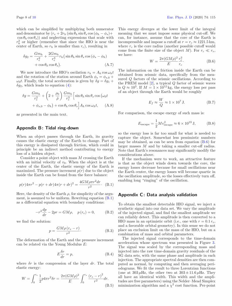
which can be simplified by multiplying both numeratorand denominator by (re + 2rh (sin θh sin θs cos (φh − φs)+cos θh cos θs)) and neglecting expressions that scale withr2h or higher (remember that since the HIO is near the

center of Earth, so rh is smaller than re), resulting in

δg2 =Gmh

r2e

+2Gmh

r3e

rh(

sin θh sin θs cos (φs − φh)

+ cos θh cos θs). (A.7)

We now introduce the HIO’s oscilation rh = Ah cosωhtand the rotation of the station around Earth φs = φs,0 +ω0t. Finally, the total acceleration is given by δg = δg1 +δg2, which leads to equation (4):

δg =Gmh

r2e

+(

2 +ρ0

ρ

)Gmh

r3e

[sin θh sin θs cos

(ω0t

+ φs,0 − φh)

+ cos θh cos θs]Ah cosωht, (A.8)

as presented in the main text.

Appendix B: Tidal ring-down

When an object passes through the Earth, its gravitycauses the elastic energy of the Earth to change. Part ofthis energy is dissipated through friction, which could inprinciple be an indirect method contributing to energyloss of a hidden object.

Consider a point object with mass M crossing the Earthwith an initial velocity of v0. When the object is at thecenter of the Earth, the elastic energy of the Earth ismaximized. The pressure increment p(r) due to the objectinside the Earth can be found from the force balance:

p(r)4πr2 − p(r + dr)4π(r + dr)2 =4GMρπr2dr

r2· (B.1)

Here, the density of the Earth ρ, for simplicity of the argu-ment, is assumed to be uniform. Rewriting equation (B.1)as a differential equation with boundary conditions:

−r2 dp

dr− 2pr = GMρ, p (re) = 0, (B.2)

we find the solution:

p =GMρ (re − r)

r2· (B.3)

The deformation of the Earth and the pressure incrementcan be related via the Young Modulus E:

Eδr

dr= p, (B.4)

where δr is the compression of the layer dr. The totalelastic energy:

W =∫ re

0

12p4πr2δr =

2π(GMρ)2

E

∫ re

0

(re − r)2

r2dr.

(B.5)

This energy diverges at the lower limit of the integralmeaning that we must impose some physical cut-off. Wecan, for instance, assume that the core of the Earth isincompressible and impose a cutoff at r = rc ≈ 1221.5 km,where rc is the core radius (another possible cutoff wouldcome from the finite size of the object M). For rc � re,we have:

W =2π(GMρ)2

E

r2e

rc· (B.6)

The information on the friction inside the Earth can beobtained from seismic data, specifically from the mea-sured Q factors of the seismic oscillations. According tothe PREM model [2], a typical Q factor of seismic wavesis Q ≈ 103. If M = 1× 1012 kg, the energy loss per passof an object through the Earth would be roughly

Ef ≈W

Q≈ 1× 107 J. (B.7)

For comparison, the escape energy of such mass is:

Eescape =12Mv2

escape ≈ 6× 1019 J, (B.8)

so the energy loss is far too small for what is needed tocapture the object. Somewhat less pessimistic numbersmay be obtained, as can be seen from equation (B.6) forlarger masses M and by taking a smaller cut-off radius.Note that Earth’s resonances may significantly modify theconsiderations above.

If the mechanism were to work, an attractive featureis that as the object winds down towards the core, theenergy losses decrease because for small oscillations nearthe Earth center, the energy losses will become quartic inthe oscillation amplitude, so the losses effectively turn off,enabling long “ringing” of the oscillation.

Appendix C: Data analysis validation

To obtain the smallest detectable HIO signal, we inject asynthetic signal into our data set. We vary the amplitudeof the injected signal, and find the smallest amplitude wecan reliably detect. This amplitude is then converted to aHIO mass in an optimistic orbit (i.e., one with r = 0.1 re,and a favorable orbital geometry). In this sense we do notplace an exclusion limit on the mass of the HIO, but on acombination of mass and orbital parameters.

The injected signal corresponds to the time-domainacceleration whose spectrum was presented in Figure 3.The signal was scaled by the corresponding mass andinjected into the raw time-domain gravity residuals of theSG data sets, with the same phase and amplitude in eachinjection. The appropriate spectral densities are then com-puted as normal, by computing and then averaging peri-odograms. We fit the result to three Lorentzian functions(one at 303µHz, the other two at 303± 11.6µHz. Theyall have an identical width. This width and the ampli-tudes are free parameters) using the Nelder–Mead Simplexminimization algorithm and a χ2 cost function. Per-point

Eur. Phys. J. D (2020) 74: 115 Page 9 of 10

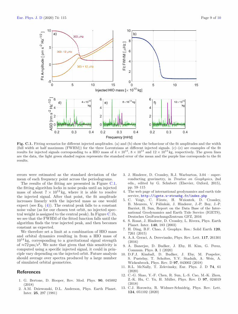
Fig. C.1. Fitting scenarios for different injected amplitudes. (a) and (b) show the behaviour of the fit amplitudes and the width(full width at half maximum (FWHM)) for the three Lorentzians at different injected signals. (c)–(e) are examples of the fitresults for injected signals corresponding to a HIO mass of 4 × 1013, 8 × 1013 and 12 × 1013 kg, respectively. The green linesare the data, the light green shaded region represents the standard error of the mean and the purple line corresponds to the fitresults.

errors were estimated as the standard deviation of themean of each frequency point across the periodograms.

The results of the fitting are presented in Figure C.1,the fitting algorithm locks in noise peaks until an injectedmass of about 7 × 1013 kg, where it is able to resolvethe injected signal. After that point, the fit amplitudeincreases linearly with the injected mass as one wouldexpect (see Eq. (4)). The central peak falls to a constantnoise value (as for our chosen test orbit, no injected spec-tral weight is assigned to the central peak). In Figure C.1b,we see that the FWHM of the fitted function falls until thealgorithm finds the true injected peak, and then becomesconstant as expected.

We therefore set a limit at a combination of HIO massand orbital dynamics resulting in from a HIO mass of1014 kg, corresponding to a gravitational signal strengthof ≈72 pm/s2. We note that given that this sensitivity iscomputed using a specific injected signal, it could in prin-ciple vary depending on the injected orbit. Future analysisshould average over spectra produced by a large numberof simulated orbital geometries.

References

1. G. Bertone, D. Hooper, Rev. Mod. Phys. 90, 045002(2018)

2. A.M. Dziewonski, D.L. Anderson, Phys. Earth Planet.Inter. 25, 297 (1981)

3. J. Hinderer, D. Crossley, R.J. Warburton, 3.04 – super-conducting gravimetry, in Treatise on Geophysics, 2ndedn., edited by G. Schubert (Elsevier, Oxford, 2015),pp. 59–115

4. The web page of international geodynamics and earth tideservice, http://igets.u-strasbg.fr/index.php

5. C. Voigt, C. Forste, H. Wziontek, D. Crossley,B. Meurers, V. Palinkas, J. Hinderer, J.-P. Boy, J.-P.Barriot, H. Sun, Report on the Data Base of the Inter-national Geodynamics and Earth Tide Service (IGETS),Deutsches GeoForschungsZentrum GFZ, 2016

6. S. Rosat, J. Hinderer, D. Crossley, L. Rivera, Phys. EarthPlanet. Inter. 140, 183 (2003)

7. H. Ding, B.F. Chao, J. Geophys. Res.: Solid Earth 120,7261 (2015)

8. A.A. Geraci, A. Derevianko, Phys. Rev. Lett. 117, 261301(2016)

9. A. Banerjee, D. Budker, J. Eby, H. Kim, G. Perez,Commun. Phys. 3, 1 (2020)

10. D.F.J. Kimball, D. Budker, J. Eby, M. Pospelov,S. Pustelny, T. Scholtes, Y.V. Stadnik, A. Weis, A.Wickenbrock, Phys. Rev. D 97, 043002 (2018)

11. R.L. McNally, T. Zelevinsky, Eur. Phys. J. D 74, 61(2020)

12. C.-G. Shao, Y.-F. Chen, R. Sun, L.-S. Cao, M.-K. Zhou,Z.-K. Hu, C. Yu, H. Muller, Phys. Rev. D 97, 024019(2018)

13. C.J. Horowitz, R. Widmer-Schnidrig, Phys. Rev. Lett.124, 051102 (2020)

Page 10 of 10 Eur. Phys. J. D (2020) 74: 115

14. K. Lawson, X. Liang, A. Mead, M.S.R. Siddiqui, L.Van Waerbeke, A. Zhitnitsky, Phys. Rev. D 100, 043531(2019)

15. A.R. Zhitnitsky, J. Cosmol. Astropart. Phys. 2003, 010(2003)

16. E. Roche, Acad. Sci. Montpellier 1, 1847 (1850)17. D. Wittman, N. Golovich, W.A. Dawson, Astrophys. J.

869, 104 (2018)18. D. Crossley, J. Hinderer, G. Casula, O. Frnacis, H.-T. Hsu,

Y. Imanishi, G. Jentzsch, J. Kaarianen, J. Merriam, B.Meurers, J. Neumeyer, Eos Trans. Am. Geophys. Union80, 121 (1999)

19. J.-P. Boy, Description of the level 2 and level 3 IGETS dataproduced by EOST (2019), https://isdc.gfz-potsdam.de/igets-data-base/documentation/

20. S. Rosat, J. Hinderer, Sci. Rep. 8, 15324 (2018)

21. M. Mikolaj, M. Reich, A. Guntner, J. Geophys. Res.: SolidEarth 124, 2153 (2019)

22. S. Rosat, S. Watada, T. Sato, Earth Planets Space 59, 307(2007)

23. T.G. Masters, R. Widmer, Free oscillations: frequenciesand attenuations, in Global Earth Physics: a handbook ofphysical constants (1995), Vol. 1, p. 104

24. LIGO Scientific Collaboration, Virgo Collaboration, et al.Class. Quantum Grav. 37, 055002 (2020)

25. S. Afach, D. Budker, G. DeCamp, V. Dumont, Z.D.Grujic, H. Guo, D.F. Jackson Kimball, T.W. Kornack, V.Lebedev, W. Li, H. Masia-Roig, S. Nix, M. Padniuk, C.A.Palm, C. Pankow, A. Penaflor, X. Peng, S. Pustelny,T. Scholtes, J.A. Smiga, J.E. Stalnaker, A. Weis, A.Wickenbrock, D. Wurm, Phys. Dark Univ. 22, 162 (2018)

26. A. Derevianko, Phys. Rev. A 97, 042506 (2018)