A Network View on Interbank Liquidity ∗

Silvia Gabrieli†

Banque de France

Co-Pierre Georg‡

University of Cape Town

Deutsche Bundesbank

June 23, 2016

Abstract

The euro area overnight interbank market is best described as a network of over-the-counter

lending relationships. We study liquidity reallocation in this interbank network using a novel

dataset of all interbank loans settled between European banks. We show the existence of a

network pricing channel in over-the-counter markets: a bank’s importance in the interbank net-

work, measured by its centrality, has an economically significant effect on its liquidity provision

and access. The effect is stronger for the price of liquidity than for the volume, and stronger for

liquidity provision than for liquidity access.

Keywords: interbank networks, liquidity, network formation

JEL Classification: D85, E5, G1, G21

∗We wish to thank Viral Acharya, Franklin Allen, Jean-Edouard Colliard, Adam Copeland (discussant), Jefferson Duarte (discussant), Darrell

Duffie, Falko Fecht, Craig Furfine (discussant), Grzegorz Halaj (discussant), Rajkamal Iyer, Marco van der Leij, Iman van Lelyveld (discussant),

Robin Lumsdaine (discussant), David Musto (discussant), Michael Papageorgiou, Christophe Perignon (discussant), Dilyara Salakhova (discussant),

Antoinette Schoar, and Sascha Steffen, as well as conference and seminar participants at the 2016 AFA Day Ahead Conference, 2015 Mitsui Finance

Conference, FIRS 2015, 2014 Bundesbank/DIW/ESMT Conference, Isaac Newton Institute for Mathematical Sciences Workshop at Cambridge

University, FDIC 13th Annual Bank Research Conference, 2013 ECB Money Market Workshop, 2013 CEPR Workshop on the Economics of Cross-

Border Banking, the 7th Financial Risks International Forum, University of Wisconsin Business School, DIW, Banco Central do Brazil, Deutsche

Bundesbank, University of Vienna, the Tinbergen Institute, Banca d’Italia, and the Federal Reserve Bank of New York for valuable comments and

suggestions. Opinions expressed in this paper do not necessary reflect the views of the Eurosystem or its staff.†E-Mail: silvia.gabrieli@banque-france.fr‡Corresponding author. E-Mail: co-pierre.georg@bundesbank.de

1 Introduction

The overnight interbank market is a decentralized over-the-counter (OTC) market for central bank

reserves, and a major source of liquidity for euro area banks.1 Consequently, the smooth and

cost-efficient reallocation of liquidity in the interbank market is key for the resilience of the finan-

cial system and the implementation of the monetary policy stance, especially during periods of

large adverse shocks. Banks borrow and lend on the overnight interbank market multiple times

during a day and act as intermediaries between banks with a liquidity surplus and banks with a

liquidity deficit. Thus, the euro area interbank market is best described as a network of interbank

loans amongst banks. However, contracts are bilaterally negotiated and information about trading

partners, volumes, and prices is usually not available.2

We use a novel and uniquely detailed dataset of all interbank loans settled among any two

euro area banks around the Lehman event to study the effect of the interbank network structure

on the price and volume of banks’ liquidity provision and access. To build some intuition, assume

that the only difference between two banks is that the first is able to borrow from counterparties

who, themselves, have more counterparties to borrow from. Even if both have the same number

of counterparties, the first is at an advantage. If hit by a liquidity shock, it can obtain liquidity

from counterparties who, in turn, can obtain liquidity from a larger number of possible lenders.

We formalize this intuition and the notion of a pivotal bank using measures of a bank’s network

centrality. A bank’s betweenness centrality, for example, is measured as the fraction of all shortest

paths of liquidity intermediation between any two banks that pass through this bank.

Using loan-level data, and controlling for demand, we show in Section 4 that banks with a

more pivotal position in the interbank network make significantly larger intermediation spreads and

provide more liquidity. The effect is beconomically large: A one one standard deviation increase in1On average, interbank lending accounts for over 25% and interbank borrowing for roughly 21% of total asset size

in the euro area in 2008 (see European Central Bank (2009)).2A notable exception is the Italian e-MID trading platform. Banks voluntarily choose whether or not to trade in

a transparent way using e-MID. However, since only the most viable banks will choose to trade transparently, e-MIDlikely suffers from a self-selection bias. In addition, e-MID only covered about 14% of the turnover in the euro areainterbank market before the crisis, most of which involved Italian banks only.

1

betweenness centrality, for example, leads to an almost 30% increase in the intermediation spread

a bank is able to capture and a 2% increase in liquidity provision. In Section 5 we show that this

network pricing channel of liquidity provision arises because banks with higher network centrality

have access to more and cheaper liquidity. Using bank-level regressions with a bank’s network

centrality in a reference period–to avoid issues of reverse causality–as independent variable, we

show that banks with a one standard deviation increase in betweenness centrality pay 34% less for

their interbank borrowing.

Our main contribution is to the literature on trading in over-the-counter markets. Search

models of OTC markets assume a continuum of atomistic agents that have a zero probability of

meeting more than once (see, for example, Duffie et al. (2005), Duffie et al. (2007)). Such models

abstract from the network character of the market. We show, however, that the network structure

can have a sizeable effect on pricing. Our paper, therefore, mainly contributes to the growing

literature on trading in OTC networks (see, for example, Gale and Kariv (2007), Gofman (2011),

Condorelli and Galeotti (2012), Babus and Kondor (2014), Farboodi (2014), Manea (2016), and

Malamud and Rostek (2016)).

While empirical evidence is still scarce, an emerging literature studies the network structure

of municipal (Li and Schuerhoff (2014)) and corporate (di Maggio et al. (2015)) bond OTC markets.

In line with our results, and the theoretical predictions of Babus and Kondor (2014), di Maggio et al.

(2015) find that central dealers make larger intermediation spreads and intermediate more. Similarly,

Li and Schuerhoff (2014) find that central dealers charge a higher spread but provide immediacy to

customers. Our paper differs from this literature because we study the euro area overnight interbank

market, which is not only crucial for financial stability, but also for the implementation of monetary

policy in the euro area.

Our paper relates local liquidity provision, the formation of new lending relationships between

banks, with the existing global structure of the interbank network, which, in addition to the reasons

outlined above, is important for at least five reasons. First, understanding how interbank networks

form and evolve over time is of particular importance during times of distress when a shortage

2

of interbank liquidity can trigger costly fire-sales and thus impair financial stability. Second, ac-

cess to interbank liquidity directly affects provision of credit to the real economy (see Khwaja and

Mian (2008) and Iyer et al. (2014)). Third, interbank linkages create a counterparty risk exter-

nality (see Acharya and Bisin (2014)). This externality is at the heart of models of contagion in

interbank networks (see, amongst others, Zawadowski (2013), Elliott et al. (2014), Acemoglu et al.

(2015)). Fourth, interbank lending implements, as Rochet and Tirole (1996) point out, a form of

peer monitoring. Whether or not a link is formed affects market discipline and efficiency. Fifth, our

hypotheses provide empirical guidance for models of interbank network formation (recent examples

in this literature include Farboodi (2014) and Gofman (2011)).

We use novel and unique data on all unsecured interbank loans settled between any two

European banks between July and December 2008 obtained from TARGET2, the euro area’s large

value payment system.3 Interbank loans are identified using the algorithm originally developed by

Furfine (1999) in the implementation of Arciero et al. (2013).4 Because we have information on the

ultimate originator and final beneficiary of each transaction, the typical identification problem of

false positives is much less prevalent in our data. This allows us to extract interbank loans from the

raw set of payments with unprecedented accuracy. We split our sample in five periods, with a two

week window at the beginning of the sample, before and after the Lehman insolvency, following the

Eurosystem’s first special refinancing operation that was conducted as a full-allotment tender, and

following the change to a full-allotment regime of monetary policy.

As a first step in our analysis, we study the structure of the euro area overnight interbank

market before and after the Lehman event in Section 3. Empirical studies show that domestic3In 2012 TARGET2 settled 92% of the total large-value payment system traffic in euro. The remaining fraction

of the total turnover is settled mostly via the EURO1 payment and settlement system (see European Central Bank(2013)). The settlement of secured interbank loans involves central counterparties which we drop from our data toensure that we only consider unsecured interbank loans.

4This implementation is extensively tested and verified using data on actual interbank transactions obtainedfrom the e-MID trading platform in Italy and the Spanish MID trading platform. This verification reveals that theimplementation of the Furfine algorithm used in this paper correctly identifies about 99% of all e-MID trades, andover 90% of all trades reported in MID. Concerns regarding the identification quality of the Furfine algorithm arevoiced Armantier and Copeland (2016). However, Kovner and Skeie (2013) show that the identified interbank loansshow a statistically significant correlation with interbank loans reported on the FRY-9C, which indicates that theFurfine algorithm can indeed be used to identify interbank loans.

3

interbank networks tend to have a core-periphery structure, i.e. are comprised of a small group of

highly connected banks (the core) and a large group of banks (the periphery) which is only connected

through the core.5 The euro area overnight can be described as a core-periphery network, albeit

with a higher error score than e.g. the German interbank network. There is substantial variation

between the pre-Lehman and the post-Lehman interbank network structure–roughly 60% of all links

change between those periods.

We find, somewhat surprisingly, a significant increase in interbank lending following the

Lehman event. This can best be understood in the context of asymmetric information. Glode

and Opp (2016) study intermediation chains as a means to overcome large asymmetric information.

The key result of their model is that an increase in asymmetric information leads to an increase

in trading activity before asymmetric information ultimately becomes too large and the market

breaks down. We complement this analysis in Section 6 by directly comparing the price and volume

dynamics in the euro area with the developments in the fed funds market, studied in Afonso et al.

(2011). The increase in overnight interbank lending is accompanied by a slight decrease in interbank

lending in the term segment for loans with a maturity longer than overnight and up to one year.

Similarly to the US, lenders in the overnight market become sensitive to borrower characteristics,

i.e. to counterparty risk. In the term segments, on the other hand, lending dropped irrespective of

borrower or lender characteristics.

Our paper contributes to various other streams of literature. First, most papers that study the

interbank network structure study only global network properties. To the best of our knowledge, no

paper studies whether the global network structure has an impact on the local provision and access

of liquidity. Second, we provide empirical guidance for the rapidly growing theoretical literature

that studies the formation and efficiency of interbank networks (see, amongst many others, Leitner

(2005), Gofman (2011), Farboodi (2014), Babus and Kondor (2014), in’t Veld et al. (2014), Blasques

et al. (2014), and Colliard and Demange (2015)). Third, the literature on the bank-lending channel

(see, for example, Khwaja and Mian (2008), Iyer et al. (2014)) studies the impact of interbank5See, for example, Craig and von Peter (2014) for a study of the German interbank market.

4

liquidity shocks on credit provision. We study heterogeneity in the access to interbank liquidity

based on a bank’s position within the interbank network, a dimension that has not been studied

in the literature. And fifth, studying the dynamics of liquidity provision during times of distress

contributes to the literature on money market freezes. Our results are in line with Afonso et al.

(2011), who show that the overnight segment of the fed funds market in the United States was

“stressed, but not frozen”. Acharya and Merrouche (2013) document that large settlement banks

in the UK hoarded liquidity precautionary, following the first period of heavy turmoil in euro area

interbank markets in August 2007. Heider et al. (2015) show that during times of large asymmetric

information banks anticipate a dry-up of interbank lending and start hoarding liquidity as a result.

Acharya and Skeie (2011) and Acharya et al. (2011) develop a model of interbank markets with

precautionary demand for liquidity. Our contribution is that we add a cross-sectional, structural,

perspective to the aggregate perspective taken in the literature.

2 Characterizing a Bank’s Position in the Interbank Network

It is useful to introduce the notation used to characterize a bank’s position in the interbank network

first. A network G is a set of nodes together with a set of links between the nodes. We are

interested in interbank networks, each node is thus a bank and each link is a loan from one bank

(the originator) to another bank (the beneficiary). The network is represented by an adjacency

matrix g with gij = 1 whenever bank i has given a loan to bank j and gij = 0 otherwise.6 A loan

from bank i to bank j on day t is denoted as Loanij,t and interbank market turnover on day t is

thus given as:

Loant =∑i

∑j

Loanij,t. (1)

We study liquidity provision and access along four dimensions: access, amount, price, and

number of counterparties. The extensive margin of liquidity access is given by Accessi,t, which6Technically, the adjacency matrix can contain the value of the loan from i to j as weight. We use the unweighted

network, unless noted otherwise, since the weight is captured by Loanij,t.

5

equals one if we take a borrower perspective and bank i borrowed on the interbank market on day

t, i.e.:

Accessbi,t = maxj{gji,t}, (2)

where the superscript b indicates access to interbank borrowing. If we take a lender perspective

and bank i lends on the interbank market on day t we denote i’s willingness to lend as Accessli,t =

maxj{gij,t}.

To study the intensive margin of liquidity access, we define the amount borrowed by bank i

on day t as:

Amounti,t =∑j∈Bi,t

Loanji,t, (3)

where Bi,t = {j|gji,t = 1} is the set of banks j that lend to bank i on day t. Similarly, Li,t =

{j|gij,t = 1} is the set of banks j to which bank i lends on day t.

Denote the price of a loan (i.e. the overnight interest rate) from i to j on day t as pij,t and

the volume-weighted average of prices bank i pays to its lenders on day t as p̂ij,t:

p̂ij,t = pij,t ×Loanij,t∑

j∈Li,t Loanij,t. (4)

The spread to the mean interbank interest rate that borrower i pays on the interbank market on

day t is defined as:

Spreadbi,t =

∑j∈Li,t

p̂ji,t − p̂t. (5)

where p̂t is the average interbank interest rate on day t, p̂t =∑

i

∑j∈Li,t p̂ij,t. Finally, we use

the number of counterparties of bank i using the nomenclature defined above. Bank i’s asset-side

diversification Degreeli,t is defined as the number of counterparties j to which i has a loan on day t:

Degreeli,t = |Li,t| (6)

Equivalently, a bank’s liability side diversification Degreebi,t is given by the number of counterparties

6

j that have granted an interbank loan to i on day t. Asset side diversification of a bank i is also

denoted as bank i’s out-degree, while liability side diversification of bank i is also denoted as i’s

in-degree. Following this nomenclature, we sometimes denote the amount bank i borrows from

others as i’s weighted in-degree and the amount bank i lends to others as i’s weighted out-degree.

Before we can address the question if a bank’s position in the interbank network affects

liquidity provision and access, we have to specify in more detail which network we are using. There

are two ways to specify what it means for banks to be connected in a network. The first, and

straightforward way, is to use the daily networks of newly established interbank loans Gt (i.e. the

daily turnover networks), compute the relevant network measures, and then average them over a

sample period. The alternative is to compute the interbank network as an aggregate over a sample

period and then compute the network measures.7 In this paper, we follow the latter approach

because banks, by their very nature, engage in maturity transformation. Their lending decision

and subsequently the endogenously chosen network structure at date t depends not only on their

borrowing at t, but also on the borrowing (network structure) in t−∆t. Aggregating over a sample

period is also the more natural choice if one is interested in liquidity provision and access because

an interbank link that exists at some point during the aggregation period indicates that the two

banks in question are able to engage in interbank lending. A link in the sample period is therefore

indicative of the potential to provide and obtain liquidity. Thus, all network measures in this paper

are computed for a reference period:

Gτ =⋃t∈τ

Gt, with gij,τ =∑t∈τ

gij,t (7)

where τ is one of the sample periods defined in Section 3. The elements of the adjacency matrix

for the sample period gij,τ are thus the number of days during the sample period on which there

existed a loan from bank i to bank j.

Network theory provides a wide variety of measures to quantify a node’s position in a network7Because network measures are not additive, e.g. the betweenness on a sum of networks is different from sum of

the betweenness of the individual networks.

7

and for our analysis we select measures that have a natural economic interpretation in the context of

interbank lending. Many network measures incorporate not only information about node i’s (direct)

neighbors, but also about neighbors of neighbors and so on. We are interested in network measures

that proxy a bank’s liquidity provision and access in a given period τ . To this end, we first define

a shortest path between two banks i and j in network Gτ . A path from bank i to bank j in a

network Gτ is a sequence of banks i, . . . , j in which all banks are distinct and each bank has a link

to its successor. The length of the path is the number of banks it contains minus one. If more than

one path exists from bank i to bank j, the shortest such path is called geodesic and denoted σij,τ .

The distance dij,τ from bank i to bank j is defined as the length of the geodesic between them,

dij,τ = |σij,τ |. The average shortest path for bank i is the mean geodesic distance separating the

bank from all other banks in the network:

di,τ =

∑j∈Bi,t dji,τ

|N | − 1(8)

The average shortest path length of the network is the sum over all nodes’ individual shortest

paths divided by the number of nodes and gives the average number of links that connect any two

nodes in the network. Similarly, the diameter of the network is the length of the longest shortest

path between any two nodes in the network. The average shortest path length is a measure of the

average length of liquidity intermediation chains, while the diameter measures the length of the

longest liquidity intermediation chain.

A network is connected if there exists a path between any two nodes in the network. The

largest connected component is the largest connected set of nodes.

A very broad, but useful global measure is the network density, which is defined as the ratio of

actual links in a reference period #Loansτ to possible links. For an undirected network, the density

is defined as:

ρτ =#Loansτ

Nτ × (Nτ − 1). (9)

The most natural interpretation of network density is that it provides a simple measure of market

8

completeness, i.e. it is the probability that two randomly chosen banks can engage in interbank

lending.

The most direct measure of bank i’s liquidity provision and access is i’s betweenness centrality,

defined as the fraction of all shortest paths between any two banks j and k that pass through i:

Betweennessi,τ =

∑j∈Bi,t ajk,τ |i/ajk,τ

(|N | − 1)× (|N | − 2)(10)

where ajk,τ |i denotes the number of geodesics between j and k that contains i, ajk,τ is the total

number of geodesics between j and k.8 The betweenness of bank i is a proxy for how easy it is for this

bank to access liquidity in the interbank market, i.e. accessing a random Euro of liquidity flowing

between any two banks in the market. It is also a direct measure for a bank i’s intermediation

function. Banks with high betweenness are in a larger number of intermediation chains. Thus,

they are more relevant for financial intermediation, as a shock at such pivotal banks will affect the

smooth flow of funds more strongly.

As a robustness check, we will also use the Katz centrality, which computes the relative

influence of bank i within a network by measuring the number of its immediate neighbors (lenders)

and also of all other banks in the network that lend to bank i through these immediate neighbors.

The Katz centrality for bank i is defined as:

Katzi,τ = α∑j∈Bi,t

gji,τ + β (11)

where gji,τ is the adjacency matrix representing the network with eigenvalues λ, and β = 1. The

parameter α ≤ 1/λmax is an attenuation factor that allows to penalize loans made amongst distant

neighbors, i.e. with neighbors of neighbors (of neighbors of . . .) of bank i.9 Moreover, extra weight

can be provided to immediate neighbours (lenders) of bank i through the parameter β, which8Dividing by (|N | − 1)× (|N | − 2) obtains a normalized version of betweenness, because this factor represents the

maximum number of pairs of banks not including i, hence the maximum value that this indicator can take.9The algorithm uses the power iteration method to compute the eigenvector corresponding to the largest eigenvalue

of g. The condition that α be less than (or equal to) the inverse largest eigenvalue of g is necessary for the algorithmto converge.

9

controls for the initial centrality.10

3 The Euro Area Interbank Market During the Financial Crisis

3.1 The Institutional Framework

Turmoil in international financial markets reached a new high when the US investment bank Lehman

Brothers filed for bankruptcy on 15 September 2008. Interbank markets in the euro area experi-

enced an unprecedented surge of risk premia, measured as the spread between the London Interbank

Offered Rate (LIBOR), and the most common proxy of a risk-free rate, the interest rate on a matu-

rity matched index rate (OIS).11 The dynamics and size of this surge in risk premia indicates that

market participants–particularly in Europe–did not anticipate the insolvency of Lehman Brothers,

which makes it a prime example for an exogenous shock to the euro area interbank market. In

response to this shock, the Eurosystem took various exceptional and unprecedented measures to

ensure the liquidity provision for European banks. On 30 September, the Eurosystem conducted

a Special Refinancing Operation (SRO) to ease banks’ mounting liquidity needs. Starting from 15

October 2008 the operational framework of monetary policy implementation was changed from the

regular variable-rate tender procedure to a fixed-rate full allotment policy which would guarantee

banks the allocation of the full amount of liquidity they demand, provided they can pledge sufficient

collateral.

We are interested in the network structure of the euro area overnight interbank market. Thus,

an in-depth analysis of actual individual banks’ transactions is required. The interbank market,

however, is an over-the-counter (OTC) market where trade details are only known to the involved

parties. Transaction level information is thus notoriously hard to obtain. One alternative to track10For α = 1/λmax, and β = 1, which are the parameter choices we make throughout, Katz centrality equals

eigenvector centrality.11The LIBOR panel is updated periodically to only include the most trustworthy banks. This implies that there

is a risk that the current LIBOR panel contains a bank which could experience distress in the future. This risk ispriced and, thus, the LIBOR-OIS spread is positive.

10

liquidity flows in the interbank market is through the way trades are actually settled. Interbank

payments (denominated in euros) are almost exclusively settled via TARGET2, the real-time gross

settlement (RTGS) system owned and operated by the Eurosystem.12 With a daily average of

354, 185 payments and EUR 2, 477 billion settled in 2012, TARGET2 is one of the largest payment

systems in the world, alongside Fedwire in the United States and the CLS multi-currency cash

settlement system.

The database we use in this paper relies on a methodology recently developed by the Eu-

rosystem allowing to identify unsecured overnight interbank loans from payments settled through

TARGET2 (see Arciero et al. (2013)). This methodology relies on a refined version of the algorithm

originally developed by Furfine (1999) to find loan-refund combinations from payment data. In its

simplest form the algorithm assumes a round value transferred from bank A to bank B at time

t and the same value plus a plausible interest rate amount from bank B to bank A at time t+1.

Among other enhancements, the refined version developed for the Eurosystem investigates several

areas of plausibility for implied interest rates (i.e. several interest rate corridors) and develops a

method to choose the most plausible duration in case of multiple loan-refund matches. Moreover,

the implementation has been comprehensively validated against actual interbank loans. Arciero

et al. (2013) report a very low Type 2 error of less than one percent for the best algorithm setup, of

which only 0.26% represent wrong matches (see Arciero et al. (2013) for more details on the sources

used for and the results of the validation).

We study the period between 04 July and 30 October 2008 and split our sample into five

different periods: The period from 28 August to 12 September is denoted the pre-Lehman period.

The period from 15 September to 29 September is denoted the post-Lehman period. On 29 September

the ECB announced a Special Refinancing Operation (SRO) which was conducted on 30 September

2008 and lasts until 14 October 2008.13 On 15 October 2008, the ECB adopted a full-allotment12In 2012 TARGET2 settled 92% of the total large-value payment system traffic in Euro. The remaining fraction

of the total turnover is settled mostly via the privately operated EURO1 settlement system. However, it shouldbe noted that as far as non-commercial payments are concerned, banks can use other settlement channels, such asautomated clearing houses and correspondent banking. See European Central Bank (2013).

13Technically, the SRO was conducted as a variable rate tender with no pre-set amount and the ECB alloted atotal of EUR120 billion out of EUR141 billion total bids.

11

regime of monetary policy, which was announced on 8 October 2008. We include dates from 15

until 30 October 2008 to have the same number of days in the pre-Lehman and the full-allotment

period. In addition, we use the period from 04 July to 21 July as an initial reference period.

3.2 Stylized Facts About the euro area Interbank Market

Volume Dynamics. The measures defined in Section 2 can be used to quantify the change

in the network structure of the euro area overnight interbank market. We use a difference-in-

differences estimation to test our main hypothesis that banks with a higher network centrality

provide more liquidity and at cheaper prices on the interbank market. For this analysis, we use the

period aggregates for the interbank networks. However, test whether banks with a higher network

centrality in a pre-determined reference period (i.e. centralities computed in an aggregated network)

have better access to liquidity, we use daily turnover. We therefore present results on the volume

dynamics of the interbank market using daily turnover.

Figure 1 shows the total daily turnover (i.e.∑

iAmounti,t where the sum runs over all banks

i borrowing on a given day t) during our sample period. For a better comparison, we have included

not only the turnover in the overnight segment, but also in the term segment for loans with a

maturity of up to one year. A slightly downward sloping trend lasts until 27 August and total daily

turnover drops from around EUR182.6bn to EUR128.9bn. In the two weeks prior to the Lehman

insolvency, turnover picks up again and is at EUR155.9bn on 12 September. Somewhat surprisingly,

though, the Lehman insolvency did not lead to a breakdown of lending in the euro market.14 Rather,

a decrease in the daily turnover of term interbank lending from EUR36.8bn on 12 September to

EUR24.9bn on 25 September is more than compensated for by an increase in daily turnover in

the overnight interbank market from EUR119.2bn to EUR160.8bn in the same period. Thus, the

volume dynamics alone provide an interesting insight in the euro area interbank market around the

Lehman insolvency: there was, similarly to the US, no interbank market freeze. However, from14This is well in line with the results by Afonso et al. (2011). Similarly, Perignon et al. (2016) document that there

was no market-wide freeze in the wholesale funding market for ceertificates of deposit.

12

the time just before the ECB conducted the special refinancing operation on 29 September, to just

before its maturity on 8 November 2008, the total daily turnover dropped by 34.5%. This reduction

stems mostly from the overnight segment, since the term segment dropped from EUR25.19bn to

EUR19.19bn in the same period, a 23.8% reduction.

Table 1 provides further information on the the daily overnight interbank networks Gt. The

aggregate picture for the turnover is reflected in the mean number of lenders, which increase by

about 12% from the pre-Lehman to the post-Lehman period, and then drop by almost 30% in the

full-allotment period.

Price Dynamics. The price of overnight interbank liquidity is shown in Table 1. The spread,

defined as the volume-weighted price of liqudity in the interbank market minus the main refinancing

rate set by the ECB, is smallest during the pre-Lehman period, with an even positive median, which

indicates that a relatively small number of banks have access to cheap liquidty, while a relatively

large number of banks have to pay a high price for their interbank liquidity. Spreads decrease

substantially once the ECB conducts the special refinancing operation and during the full-allotment

period, in line with what one would expect during times of excess supply of liquidity from the central

bank.

Figure 2 also shows price dispersion, measured as the standard deviation of the daily price

of liquidity. We show the smoothed average daily price of liquidity in the overnight and term

segment for interbank loans with a maturity of more than three months and up to one year. In the

term segment, the price of liquidity increases slightly after the Lehman insolvency on 15 September

and until the ECB moved to a full-allotment regime of monetary policy on 15 October. Price

dispersion is large, but roughly constant. Prices in the overnight segment are stable until the

Lehman insolvency. Once the ECB conducted the first special refinancing operation with full-

allotment, prices are volatile and price dispersion increases substantially. With the move to the

full-allotment regime of monetary policy on 15 October the price continues to decrease and price

dispersion remains high. In particular since 15 October the deposit facility rate is not a binding

13

floor anymore, which is an indicator for abundant liquidity in the interbank market.15

Network Dynamics. In our regressions we use measures of network centrality defined on

the networks aggregated over our sample periods. Table 2 shows summary statistics for a number

of relevant network variables. The total number of loans increase from the pre-Lehman to the post-

Lehman period by roughly 7% before it drops significantly in the SRO and full-allotment period.

From the pre-Lehman to the post-Lehman period, the number of borrowers decreases by about 5%,

while the number of lenders remains roughly constant: fewer banks obtain more liquidity through

more linkages from a roughly constant number of lenders. This behavior is consistent with lender

concerns about borrower quality, which is in line with the development in the fed funds market,

studied by Afonso et al. (2011). While not the main focus of our paper, we expand this analysis in

Section 6 and the Supplementary Information B.1.We show that the euro area overnight interbank

market was characterized by lender concerns about borrower characteristics around the time of the

Lehman insolvency.

As a result of this process, the network density ρτ slightly increases from the pre-Lehman

to the post-Lehman period, the average shortest path length slightly decreases, and the diameter

decreases from 9 to 7. The size of the largest connected component increases slightly, while the share

of nodes in the largest connected component remains very high with over 98% of banks being part of

the largest connected component. Betweenness and Katz centrality decrease slightly, although this

global decrease does not yet reveal the heterogeneity across banks. The number of borrowers and

lenders continuously decrease, from the pre-Lehman to the full-allotment period by around 13%.

The density decreases by around 10%, while the average shortest path length increases by around

5% and the diameter remains constant at 7. Betweenness and Katz centrality substantially decline

by 33% and 21% from the pre-Lehman to the full-allotment period, respectively.

Using measures from network theory is only one possibility to quantify the change in the

interbank network structure, though. Another possibility is to measure in how far the observed15See Bech and Klee (2011) for a discussion of how abundant liquidity in the federal funds market can render the

floor of the federal funds rate, implemented through interest on reserves akin to the Eurosystem’s deposit facilityrate, imperfect.

14

structure of the euro area overnight interbank market corresponds to other empirically observed

interbank network structures. Empirical studies of interbank networks find that they tend to have a

core-periphery stucture in which a subset of banks (the core) is highly interconnected, and a different

subset of banks (the periphery) is connected only to the core. We identify core- and periphery nodes

following the methodology of Craig and von Peter (2014). The euro area overnight interbank market

has 732 banks with 3936 loans. The size of the core in the pre-Lehman period is 25 (and the size of

the periphery thus 707). In the pre-Lehman period, there are 253 links within the core, 1650 links

within the periphery, and 2033 links between the core and the periphery. The interbank network

in the pre-Lehman period is thus not following a clean core-periphery structure and the error score

defined by Craig and von Peter (2014) is 0.507, while the error score for the German interbank

network has an error score of only 0.12.16 In the post-Lehman period there are only 617 of the

banks in the periphery active and there are 232 links within the core, 2070 links between the core

and periphery, and 1755 links within the periphery. The error score slightly increases to 0.52 in

the post-Lehman period. Both, the core and the periphery shrink between the pre-Lehman and the

post-Lehman period, but the periphery shrinks more.

Another useful possibility to study the change of a network is to define a measure of the

structural persistence based on individual transactions, which can be quantified using the Jaccard

index J(Lτ , Lτ ′) where Lτ and Lτ ′ are subsets of the set of unweighted links in networks Gτ and

Gτ ′ , respectively.17 Recall that an link li,j ∈ L iff gij > 0. In its most general form the Jaccard

index measures how similar two sets of links are, and is defined as:

J(Lτ , Lτ ′) =

∣∣∣∣Lτ ∩ Lτ ′Lτ ∪ Lτ ′

∣∣∣∣ . (12)

We measure the Jaccard index on subsets of links in the pre-Lehman and post-Lehman period,

since this is the main exogenous shock we study.18 The Jaccard-Index yields 0.4 for the comparison16One difference between our data and the data used in Craig and von Peter (2014) is that we have daily data from

payment systems and for the overnight interbank market, while the data for the German interbank market stemsfrom the German large credit register and contains mostly term interbank lending, as Bluhm et al. (2016) show.

17The Jaccard index is defined for unweighted networks.18The Jaccard index for the post-Lehman and SRO , and the post-Lehman and full-allotment period is even smaller,

indicating even more variation in the network structure.

15

between all links, 0.54 for the comparison of links within the identified core, 0.38 for links within

the periphery, and 0.43 for links between the identified core and periphery. This means that more

than half of all links in the network change from the pre- to the post-Lehman period. As expected,

the core maintains the highest structural stability, while lending between banks in the identified

periphery is the least structurally stable.

4 Liquidity Provision and Network Position

We argue in Section 3.2 that the euro area overnight interbank market changes significantly around

the time of the Lehman insolvency. This provides us with an ideal setting to test our hypothesis that

a bank’s position in the interbank network does not affect how much liquidity the bank provides

and at what price.

When estimating the effects of liquidity provision, one concern is that the demand for inter-

bank liquidity could have been affected by the Lehman insolvency. Therefore, we construct a panel

of interbank loans that exist before and after the Lehman insolvency and use borrowing-bank fixed

effects after first-differencing the data to absorb all borrowing-bank specific demand shocks (see

Khwaja and Mian (2008)). We start from the simplified balance sheet of bank i at time t:

Other Liabilitiesi,t + Interbank Fundingi,t = Other Assetsi,t +∑j∈Li,t

Lij,t (13)

where Other Liabilitiesi,t includes demand deposits from households and firms, as well as bond and

equity financing, and Other Assetsi,t include loans to firms and households, as well as all assets

other than interbank loans. Interbank Fundingi,t is the total amount of interbank funding bank i

receives at time t. Our measure of interbank liquidity provision of bank i to bank j is denoted Lij,t.

We assume that the demand and supply of interbank liquidity is linear in each period.

Taking the first difference between two points in time obtains the equilibrium values of Lij

because of the linear model setup. We use the post- and pre-Lehman periods defined in Section 3

16

and aggregate the daily interbank networks according to Equation (7). As Khwaja and Mian (2008)

show, this model can be estimated without bias by introducing borrowing-bank fixed effects after

first-differencing. This yields our baseline regression:

∆Lij = βj + β1∆Interbank Fundingi + εij (14)

The assumption we make is that a bank’s interbank funding depends linearly on its position in the

interbank network, while its other liabilities and assets are fixed. Thus, Interbank Fundingi,τ ≡

α×Network Positioni,τ , where:

Network Positioni,τ ∈ {Amountbi,τ ,Degreebi,τ ,Betweennessi,τ ,Katzi,τ}. (15)

The first two measures, Amountbi,τ and Degreebi,τ , are local measures of a bank’s position in the

interbank network, i.e. they depend on a bank’s in-neighborhood Bi,τ only. The other two are non-

local measures that depend on the structure of the entire network. We use three different measures

Lij to measure the intensive margin of liquidity provision. First, we use the difference in the log of

interbank liquidity provided by bank i to banks j:

Amountai,τ = log

1 +∑j∈Bi,τ

Loanij,t

(16)

Second, we use the difference in the average volume weighted spread bank i charges on its interbank

lending, Spreadaij,t. And third, we use the average intermediation spread bank i makes on loans to

bank j in period τ :

Intermediation Spreadij,τ =1

|Loanij,t|∑t∈τ

Intermediation Spreadij,t (17)

where |Loanij,t| denotes the number of days on which bank i has given a loan to bank j, and the

17

intermediation spread for a loan on day t is defined as:

Intermediation Spreadij,t = pij,t × Loanij,t −∑k∈Bi,t

p̂ki,t, (18)

i.e. as the difference between the price of the loan and the volume-weighted average refinancing cost

of the lending bank i. In addition to the intensive margin of how much liquidity banks provide and at

what price, we also look at the extensive margin, i.e. if they provide liquidity at all. The extensive

margin of liquidity provision can be measured by constructing a variable Exitij for each loan in

the pre-Lehman period, which is one if the loan is no longer present in the post-Lehman period,

and zero otherwise. Similarly, we construct a variable Entryij for each loan in the post-Lehman

period, which is one if the loan was not present in the pre-Lehman period and zero otherwise. Our

borrower-bank fixed effect regression for the extensive margin is:

Exitij = βj + β1∆Interbank Fundingi + εij (19)

and similarly for Entryij . Summary statistics for the dependent variables can be found in Table 3,

summary statistics for the independent variables in Tables 4 and 5.

The coefficient of interest is always β1, which determines the strength of the interbank lending

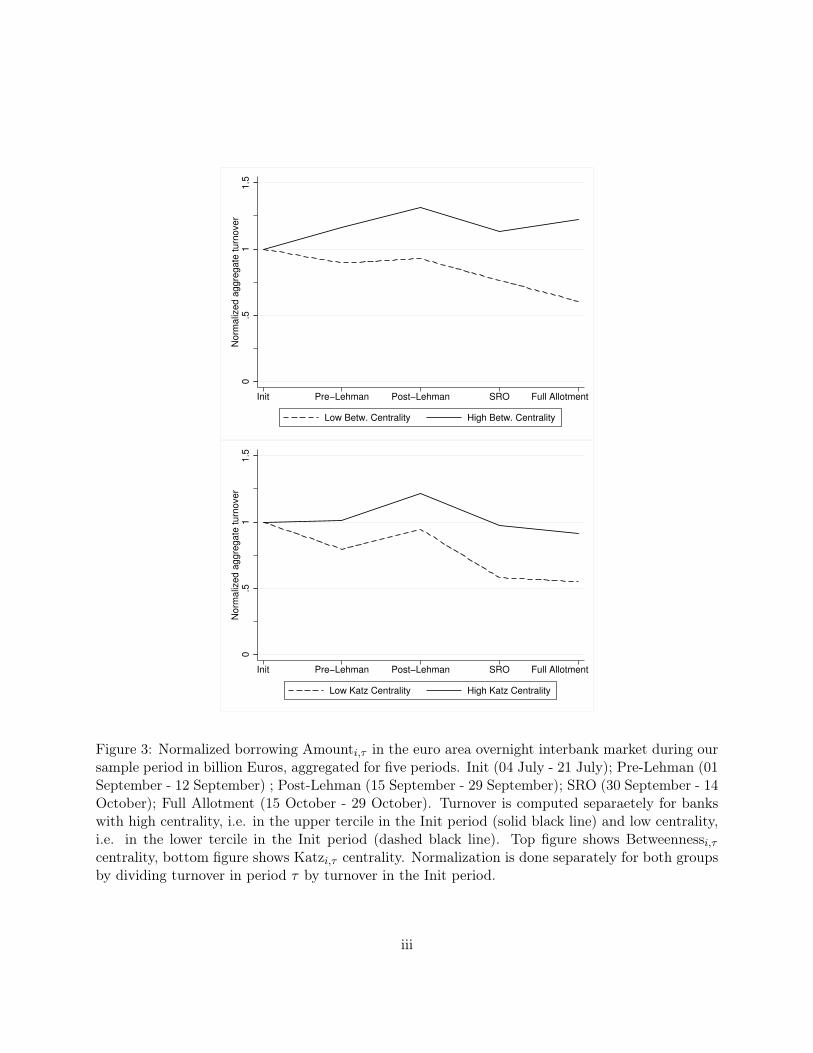
channel along the intensive and extensive margin. We start with the extensive margin of liquidity

provision, i.e. regression (19). Results for terminating an existing interbank relationship, Exitij

(see Panel A), and establishing a new interbank relationship, Entryij (see Panel B), are shown in

Table 6. We use the insolvency of the US investment bank Lehman Brothers as exogenous shock.

Results for our regression around this shock are shown in models (1) and (2), with the differ-

ence between the two models being that we include a set of lender controls in model (2). We

obtain the bank-specific control variables from bankscope and use the values reported for the

end of 2007 to avoid any reverse causality issues. We use total asset size Assetsi,2007, the loan-

loss reserves Loan Loss Reservesi,2007 as a risk proxy, and the relative size of interbank lending

18

Amounti,t/Assetsi,2007.19 Since lender controls obtained from bankscope (or SNL) are not available

for all banks in our sample, we end up with a significantly smaller sample size. The inclusion or

omission of lender controls does not change our results qualitatively, however.

One could also argue that the full-allotment special refinancing operation on 30 September

was a larger shock because it had a substantial impact on market turnover (see Section 3). Or the

shift towards a full-allotment regime of monetary policy on 15 October. To test both possibilities,

we include the respective regressions in models (3) and (4) for comparison. All three events had

massive impact on the liquidity reallocation in the euro area overnight interbank market, as Figure

1 shows. But the insolvency of Lehman Brothers, or more specifically the willingness of the US

government to let Lehman Brothers fail makes the Lehman insolvency the cleanest exogenous shock

of the three. Further evidence of this is the record height of the LIBOR-OIS spread on the day after

the Lehman insolvency, which indicates that this event was not anticipated by market participants

in Europe.

Our main results are shown in model (2) and obtained when using 15 September 2008 as

shock and when including lender controls. We find a statistically significant reduction (increase)

in the likelihood of terminating an existing (and creating a new) interbank relationship for all four

measures of liquidity provision and access. Banks are very sensitive to a reduction in interbank

lending. If interbank borrowing of bank i between the pre-Lehman and the post-Lehman period is

reduced by EUR 1m, the likelihood that an existing interbank lending relationship is terminated is

increased by 0.52%. This is stronger than the effect from losing one existing borrowing relationship

(i.e. one of bank i’s lenders is no longer willing to provide liquidity). The likelihood that an existing

interbank lending relationship is terminated when the number of lenders that lend to a bank is

reduced by one standard deviation increases by about 2.7%. Similarly, the likelihood that a new

interbank lending relationship is created is reduced by 4% when a bank’s number of lenders is

reduced by one standard deviation. Betweenness and Katz centrality have a positive, albeit smaller19We have performed a robustness check where we use non-performing loans as alternative risk proxy and all results

still hold. The coverage of loan-loss reserves on bankscope is better, however, than of non-performing loans. We havealso performed the same analysis using data from SNL instead of bankscope. All results hold, but the coverage isnot as good.

19

impact on the likelihood that an existing interbank lending relationship is terminated or created. A

one standard deviation decrease in betweenness centrality (Katz centrality) implies a 2.8% (1.4%)

increase in the likelihood that an existing interbank lending relationship is terminated, and a 1.8%

(1.3%) decrease in the likelihood that a new interbank lending relationship is created.

Table 7 shows the results of regression (14) for Amountij,t. Standard errors are clustered at

the lending-bank level. There are 3, 070 interbank loans to banks that borrow from two or more

counterparties in the pre-Lehman and post-Lehman period. Our results indicate a strong interbank

lending channel, a EUR 1m reduction in interbank liquidity provided to the lending-bank implies

a EUR 2m reduction in the amount lent. Being rationed on the interbank market thus leads to

liquidity hoarding, similar to the mechanism described in the model of Heider et al. (2015). If the

number of lenders who provide liquidity to a bank is reduced by one, the bank provides EUR 0.2m

less liquidity to the euro area overnight interbank market. A one standard deviation reduction in

a bank’s betweenness centrality implies a EUR 6.8m lower provision of liquidity, a 2.1% reduction.

The reduction of interbank liquidity provision is with 2% about the same size if a bank experiences

a one standard deviation reduction in Katz centrality.

We study the impact of a bank’s position in the interbank network on the price of liquidity

in Table 8. The price of a loan is bilaterally negotiated between the borrower and the lender and

depends on the borrower’s opportunity costs and the lender’s refinancing costs. In Panel A we show

the volume-weighted spread a bank receives for its interbank liquidity. Banks with better access to

the interbank market, i.e. banks with higher network centrality provide liquidity at cheaper prices,

measured as the difference of the volume-weighted price of liquidity p̂i,τ minus the ECB’s main

refinancing rate during period τ . Banks that, for example, experience a one standard deviation

increase in betweenness centrality provide liquidity on average 2.5bp cheaper. This is a sizeable

effect, given that the mean spread in the pre-Lehman period was −3.2bp.

In the pre-Lehman period, banks make a mean intermediation spread of about 90bp. Panel

B in Table 8 shows that the volume-weighted intermediation spread is increased by about 30bp

for banks that experience a one standard deviation increase in betweenness centrality, i.e. a 30%

20

increase.

These effects are sizeable and show that a lending-bank’s position in the interbank market

implies a sizeable interbank lending channel, in particular for the price of liquidity. Our findings

thus have direct consequences not only for financial stability, but also for the implementation of

monetary policy.

5 Interbank Network Position and Access to Liquidity

One hypothesis why banks with a more central position in the interbank network provide more

and cheaper liquidity to their counterparties is that they have access to more and cheaper liquidity

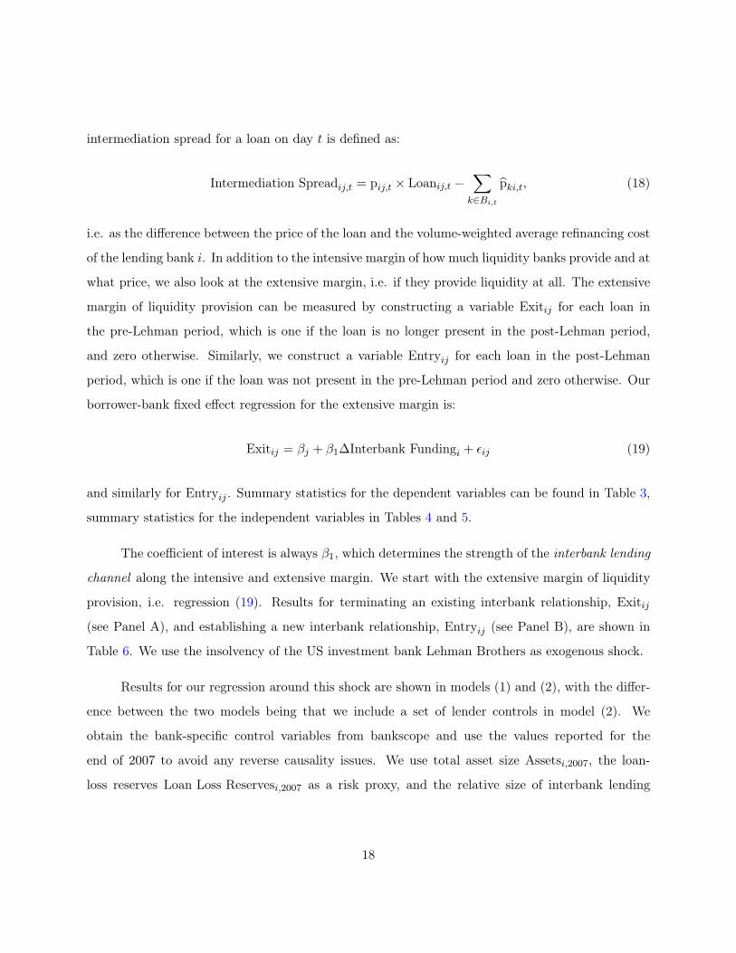
themselves. A first indication for this hypothesis can be seen in Figures 3 and 4 where we show

the amount banks borrow in interbank market and the volume-weighted spread they pay for their

interbank borrowing for two groups of banks: those in the upper and lower tercile of centrality

(betweenness and Katz centrality) in the initial period. In Figure 3 we normalize the borrowing

Amounti,τ by borrowing in the initial period. The aggregate amount the two groups borrow diverges

over time, both for Betweenness and Katz centrality. The volume-weighted spread for banks with

high centrality is below the volume-weighted spread that banks with low centrality pay, except in

the full-allotment period when banks with higher centrality pay a slightly higher price for their

interbank borrowing. We formalize this intuition and test the following hypothesis:

Banks with higher betweenness and Katz centrality do not have better access to liquidity,

measured as the amount and price of liquidity obtained, in the euro area overnight interbank

market.

by estimating a simple OLS model:

Ai,t = β0(Date) + β1 (Date×Assetsi,2007) + β2 (Date× Loan Loss Reservesi,2007) (20)

+β3

(Date× Amounti,t

Assetsi,2007

)+ β4(Date×Network Positioni,initial)

21

where liquidity access, Ai,t, is measured along three dimensions, Amounti,t, spread Spreadi,t, and

the number of loans obtained, Degreebi,t. We introduce a time-period dummy, Date, for every period

and use a set of bank-specific control variables which we obtain from bankscope.20 The advantage

of estimating such an OLS model is that it allows us to study the role of bank characteristics, which

we could not do in the Diff-in-Diff setting in Section 4 because of the relatively smaller number of

loans that can be used in the Diff-in-Diff setting.

Our main explanatory variable is Network Positioni,initial and we use the network Ginitial, i.e.

the euro area overnight interbank network in the initial period. By using only pre-determined vari-

ables, we avoid issues of reverse causality. Our two main explanatory variables are Betweennessi,initial,

and Katzi,initial centrality. In the Supplementary Information B.1 we also use local measures of liq-

uidity access, i.e. the weighted and unweighted in-degree of bank i in the reference period.

Tables (9) and (10) show the results of our estimation. Model (1) is a baseline regression

with only period dummies and control variables. The main explanatory variable is added in model

(2) and the difference between models (1) and (3) is that we add interactions between the period

dummies and the control variables in model (3). Finally, in our main specification, model (4), we

add a further interaction between the period dummies and our main explanatory variable to study

whether it acts differently in different periods.

We turn to amount borrowed first. Table (9) shows that, first, banks borrow significantly

more in the post-Lehman period, and significantly less in the full-allotment period than in the

initial period if we include borrower control times period fixed-effects. Second, larger banks obtain

more liquidity than smaller banks. Third, riskier banks, i.e. banks with higher loan-loss reserves

obtain less liquidity. And fourth, banks that have a higher share of interbank lending relative

to total assets obtain more liquidity. In line with our hypothesis, all pre-determined explanatory

variables that describe a bank’s centrality in the network are significant and positively correlated20We have performed a robustness check where we use non-performing loans as alternative risk proxy and all results

still hold. The coverage of loan-loss reserves on bankscope is better, however, than of non-performing loans. We havealso performed the same analysis using data from SNL instead of bankscope. All results hold, but the coverage isnot as good.

22

with the amount of liquidity a bank obtains in the euro area overnight interbank market.

We find a 10% increase in a bank’s betweenness (Katz) centrality in the Inital period cor-

responds to a 3.5% (1.9%) increase in the amount borrowed subsequently. The interaction of

betweenness centrality with period dummies reveals that the effect is significantly stronger in the

post-Lehman period than in the SRO and full-allotment period. For Katz centrality, the interaction

shows a more than twice as large effect in the post-Lehman period than on average.21

Banks with a better network position do not only obtain more liquidity, they also obtain it

at a cheaper price. Relative to the initial period, spreads are significantly higher in the pre-Lehman

period, but significantly lower in the full-allotment period across almost all specifications. Banks-

specific controls have very little impact on price, highlighting that the overnight interbank market

mainly uses reserves to balance short-term liquidity fluctuations. Despite this, network variables do

have an impact on the price of liquidity: A 10% increase in a bank’s betweenness (Katz) centrality

in the initial period leads to a 3.5% (5.6%) lower spread subsequently. The impact of all network

variables is stronger in the post-Lehman period.22

Overall, we find strong evidence to reject the hypothesis that banks with a more central

position in the interbank network do not have better access to liquidity in the euro area overnight

interbank market.

6 Do Borrower or Lender Characteristics Determine Liquidity Pro-

vision and Access?

We use the Lehman insolvency as exogenous shock to show that more pivotal banks not only provide

more liquidity and at cheaper prices, but also have access to more and cheaper liquidity themselves.

What remains to be seen, however, is whether the volume and price dynamics we describe in21For a comparison with the effect of local network measures, i.e. the weighted and unweighted in-degree, as well

as an analysis of access to liquidity measured by the number of borrowers, see the Supplementary Information (B.1).22For comparison: A 10% increase in the number of lenders a bank borrows from in the initial period translates

into a 7.1% lower spread, while a 10% increase in the amount borrowed leads to a 3.3% lower spread.

23

Section 3 are driven by borrower or lender characteristics. To remedy this, we directly compare the

developments in euro area interbank market with those in the fed funds market in the US around

the Lehman insolvency. Afonso et al. (2011) show that, while the overnight fed funds market did

not freeze following the insolvency of Lehman brothers, it experienced considerable stress. The

only evidence of an actual market freeze in the fed funds market is that on Monday 15 September

banks borrowed significantly less from significantly fewer counterparties when borrower fixed effects

are included. This finding is consistent with a market that is characterized by counterparty risk,

i.e. lenders are sensitive to counterparty properties. However, the overall picture for the fed funds

market does not suggest a massive market freeze in the overnight segment, at least from an aggregate

perspective.

In this section, we use data consisting of transactions with maturities from overnight to 12

months, which allows us a more nuanced view at the developments in the euro area interbank

market. We first look at the effect of the Lehman insolvency on borrowers in the overnight segment,

shown in Table 12. The sample period runs from 04 July to 30 October 2008. Model (1) is a simple

probit model with the dependent variable being equal to one if a bank accessed the interbank market

on a given day and zero otherwise. The overnight segment shows a decrease in the probability of

access relative to the initial reference period (i.e. relative to the period from 04 to 21 July) already

in the pre-Lehman period. The reduction is stronger, though, in the two days following the Lehman

insolvency. In the post-Lehman period, access is reduced, but not as strongly. Access is further

reduced in the full-allotment period. In models (2) and (3) we estimate the amount a bank borrows

on the interbank market in the various periods with and without borrower fixed effects. Without

controlling for fixed borrower characteristics, and similar to the US, we do not see any significant

reduction in trading in the overnight segment.

However, when borrower fixed effects are included, we see a significant reduction in the amount

borrowed, but only once the ECB conducted the first full-allotment special refinancing operation

and, more importantly, once full-allotment is implemented: in the latter case, the large point

estimate suggests that certain banks reduced their recourse to interbank funding by more than

24

90%. Spreads are analyzed in models (4) and (5). They are computed as the difference between

the volume-weighted average interest rate paid by a given borrower and the minimum bid rate of

the Eurosystem’s Main Refinancing Operations (MRO). Spreads were higher already in the pre-

Lehman period, but substantially more so on 15 September, when banks paid on average 0.15 basis

points more than in the initial reference period to obtain liquidity. Borrowing spreads increased by

additional 0.05 basis points on 16 September, and are slightly higher when controlling for borrower

characteristics. Then, starting in the post-Lehman period, spreads are reduced and significantly so

during the full-allotment period. The number of counterparties a bank borrows from is shown in

models (6) and (7). It is significantly lower in the pre-Lehman period and on Tuesday 16 September,

when a bank could borrow from about one counterparty less than in the reference period, and

then even more following the special refinancing operation, but only if borrower fixed effects are

considered. This shows that immediately after the Lehman insolvency lenders in the overnight

interbank market become indeed sensitive to counterparty properties. The effect is stronger with

the onset of the ECB emergency measures. Then, especially after full-allotment, bank characteristics

are important for the amount a bank borrows and the number of counterparties it borrows from.

The overall picture for the overnight segment is thus very similar to the US, with the interbank

market being stressed, but not frozen.

Was there no market freeze in Europe at all? A closer look at the term segment in Table 12

reveals a significant and sizeable impact of the Lehman insolvency. From Monday 15 September

onwards, access is significantly reduced and neither the SRO nor full-allotment can restore market

activity to pre-Lehman levels.23 A similar picture emerges for the amount borrowed (models (2) and

(3)), which is substantially reduced starting from Monday 15 September and in all periods. Spreads

increased both on Monday 15 and Tuesday 16 September (models (4) and (5)), but on Monday

15 September the economic magnitude of such effect is about one fifth compared to the increase

observed in the overnight spread.24 However, differently from the overnight segment, spreads contin-23de Andoain et al. (2014) study the liquidity provision by the ECB in more detail and show that central bank

liquidity replaces the demand for liquidity by market participants.24For each term maturity the term spread is computed as the difference between the weighted average interest paid

by a borrower at that maturity and the average market rate for the same maturity. A unique spread is thereafterobtained by weigthing the various spreads with the turnover traded at the respective maturity.

25

ued to increase even after the ECB measures. Finally, the number of counterparties is significantly

reduced on 15 and 16 September, and continues to decrease post-Lehman, with the implementation

of the SRO and under the full allotment regime. In general, the effects are not sizeably different

once we introduce borrower fixed effects and are not as large as in the overnight segment. Compared

to what we observe for the overnight segment, this provides less convincing evidence of lenders’ sen-

sitiveness to borrower characteristics in the term market: the drop in turnover volume was so large

that all borrowers saw a substantial decrease in their interbank funding. Another indication that

borrower characteristics were more relevant in the overnight segment is that the explanatory power

of our regressions when borrower fixed effects are introduced increases much more in the overnight

than in the term regressions. All in all, the picture for the term segment points more clearly to a

market freeze.

On the lending side, Table 13 shows that on Monday 15 and Tuesday 16 lenders participated

less in the overnight segment and charged higher interest rates to borrowers, while we do not

observe a significant reduction in amounts lent nor in the number of counterparties. A significant

drop occurs only on Tuesday 09/16 in the term segment. Moreover, adding fixed effects for lenders

does not change the point estimates remarkably, thus suggesting that the higher spreads where

indeed driven by borrower rather than lender characteristics. Note, however, that this does not

imply that banks were not trying to increase the liquidity of their balance sheet, it just implies that

lender characteristics were not the driving force behind the increased liquidity preference.

In the Supplementary Information B.2, we extend our analysis and take a more disaggregate

view on the interbank market by introducing in the former regressions a set of bank-specific controls

and splitting the sample according to the size of the banks.

7 Conclusion

A large number of papers study the interbank network structure to quantify the risk of contagion

in interbank markets. Our paper is complementary to this literature, since we study the relation

26

between the interbank network structure and banks’ liquidity provision and access. The main result

of our paper is that a bank’s position in the interbank network, measured by various measures of

centrality in networks, has a significant impact on both the liquidity provision and access. Banks

with higher network centrality provide more liquidity and at cheaper prices. We find a similar effect

for the access to liquidity.

We mainly study the overnight segment of the euro area interbank market rather than the

term segment because our identification is cleaner for the overnight segment. However, our data

includes the term segment of the interbank market with maturities of up to one year. The dynamics

in the term segment in the aftermath of the Lehman insolvency can help to understand the dynamics

in the overnight segment. A substantial reduction in the maturity of interbank loans is reflected in

a drop in turnover in the term segment, accompanied by the documented increase in turnover in

the overnight segment. It is likely that a similar effect can explain the dynamics of the fed funds

market in September 2008. This provides the background for the somewhat surprising finding that

the overnight interbank market did not freeze, despite the widely reported turmoil in interbank

markets.

We study whether the dynamics in the overnight interbank market is driven by counterparty

risk concerns or liquidity hoarding. When analysing both the overnight and the term segment in

a similar setup to Afonso et al. (2011), we find robust indication that banks had concerns about

counterparty risk, even in the overnight segment. As a consequence, they start hoarding liquidity by

shortening the maturity of their interbank lending. The essence of this mechanism is well captured

by the model of Heider et al. (2015). A fruitful avenue for future research is to explore the interplay

between the term and the overnight interbank market in more detail.

Our analysis provides cautionary evidence for central bank intervention. Following the switch

from the variable-rate auction-based tender system to a full-allotment regime of monetary policy, the

structure of the interbank network has changed such that the recently studied models of efficiency

in networks indicate a lower efficiency. Substituting a large part of the interbank market, as the

Eurosystem has as a reaction to the Lehman insolvency, has alleviated immediate liquidity shortages,

27

the impact on market discipline and efficiency is unclear, but likely to be negative. This aspect of

the Eurosystem’s crisis measures has not been studied before but warrants attention, as the shift

to a full-allotment regime of monetary policy is still in place and discussions about a “graceful exit”

are ongoing.

28

References

Acemoglu, D., Ozdaglar, A., Tahbaz-Salehi, A., 2015. Systemic risk and stability in financial

networks. American Economic Review 105, 564–608.

Acharya, V., Bisin, A., 2014. Counterparty risk externality: Centralized versus over-the-counter

markets. Journal of Economic Theory 149, 153–182.

Acharya, V., Gale, D., Yorulmazer, T., 2011. Rollover risk and market freezes. The Journal of

Finance 66, 1175–1207.

Acharya, V., Skeie, D., 2011. A model of liquidity hoarding and term premia in inter-bank markets.

Journal of Monetary Economics 58, 436–447.

Acharya, V.V., Merrouche, O., 2013. Precautionary hoarding of liquidity and inter-bank markets:

Evidence from the sub-prime crisis. Review of Finance 17, 107–160.

Afonso, G., Kovner, A., Schoar, A., 2011. Stressed, not frozen: The federal funds market in the

financial crisis. The Journal of Finance 66, 1109–1139.

de Andoain, C.G., Hoffmann, P., Manganelli, S., 2014. Fragmentation in the euro overnight unse-

cured money market. Economics Letters 125, 298–302.

Arciero, L., Heijmans, R., Huever, R., Massarenti, M., Picillo, C., Vacirca, F., 2013. How to measure

the unsecured money market? The Eurosystem’s implementation and validation using TARGET2

data. Working Paper 369. De Nederlandsche Bank.

Armantier, O., Copeland, A., 2016. Challenges in Identifying Interbank Loans. FRBNY Economic

Policy Review. Federal Reserve Bank of New York.

Babus, A., Kondor, P., 2014. Trading and Information Diffusion in Over-the-Counter Markets.

mimeo. Central European University.

Bech, M., Klee, E., 2011. The mechanics of a graceful exit: interest on reserves and segmentation

in the federal funds market. Journal of Monetary Economics 56, 415–431.

29

Blasques, F., Bräuning, F., van Lelyveld, I., 2014. A Dynamic Stochastic Network Model of the

Unsecured Interbank Lending Market. Swift Institute Working Paper 2012-07. Swift Institute.

Bluhm, M., Georg, C.P., Krahnen, J.P., 2016. Interbank Intermediation. Deutsche Bundesbank

Discussion Paper. Deutsche Bundesbank.

Colliard, J.E., Demange, G., 2015. Cash Providers: Asset Dissemination over Intermediation Chains.

mimeo. Paris School of Economics.

Condorelli, D., Galeotti, A., 2012. Bilateral Trading in Networks. mimeo. University of Essex.

Craig, B., von Peter, G., 2014. Interbank tiering and money-center banks. Journal of Financial

Intermediation 23, 348–375.

Duffie, D., Garleanu, N., Pedersen, L.H., 2005. Over-the-counter markets. Econometrica 73, 1815–

1847.

Duffie, D., Garleanu, N., Pedersen, L.H., 2007. Valuation in over-the-counter markets. The Review

of Financial Studies 20, 1865–1900.

Elliott, M.L., Golub, B., Jackson, M.O., 2014. Financial networks and contagion. American Eco-

nomic Review 104, 3115–3153.

European Central Bank, 2009. Annual Report 2008. Annual Report of the European Central Bank.

European Central Bank.

European Central Bank, 2013. TARGET2 Annual Report 2012. Annual Report of the European

Central Bank. European Central Bank.

Farboodi, M., 2014. Intermediation and Voluntary Exposure to Counterparty Risk. mimeo. Prince-

ton University.

Furfine, C., 1999. The microstructure of the federal funds market. Financial Markets, Institutions,

and Instruments 8, 25–44.

Gale, D.M., Kariv, S., 2007. Financial networks. American Economic Review 97, 99–103.

30

Glode, V., Opp, C., 2016. Asymmetric information and intermediation chains. American Economic

Review forthcoming.

Gofman, M., 2011. A Network-Based Analysis of Over-the-Counter Markets. mimeo. University of

Wisconsin Business School.

Heider, F., Hoerova, M., Holthausen, C., 2015. Liquidity hoarding and interbank market spreads:

The role of counterparty risk. Journal of Financial Economics 118, 336–354.

Iyer, R., Peydró, J.L., da Rocha-Lopes, S., Schoar, A., 2014. Interbank liquidity crunch and the

firm credit crunch: Evidence from the 2007-2009 crisis. The Review of Financial Studies 27, 347

– 372.

Khwaja, A.I., Mian, A., 2008. Tracing the impact of bank liquidity shocks: Evidence from an

emerging market. The American Economic Review 98, 1413–1442.

Kovner, A., Skeie, D., 2013. Evaluating the Quality of Fed Funds Lending Estimates Produced from

Fedwire Payments Data. Staff Report 629. Federal Reserve Bank of New York.

Leitner, Y., 2005. Financial networks: Contagion, commitment, and private sector bailouts. The

Journal of Finance 60, 2925 – 2953.

Li, D., Schuerhoff, N., 2014. Dealer Networks. Research Paper 14-50. Swiss Finance Institute.

di Maggio, M., Kermani, A., Song, Z., 2015. The Value of Trading Relationships in Turbulent

Times. mimeo. Columbia Business School.

Malamud, S., Rostek, M., 2016. Decentralized Exchange. mimeo. University of Wisconsin.

Manea, M., 2016. Intermediation and Resale in Networks. mimeo. MIT.

Perignon, C., Thesmar, D., Vuillemey, G., 2016. Wholesale Funding Runs. HEC Paris Research

Paper. HEC Paris.

Rochet, J.C., Tirole, J., 1996. Interbank lending and systemic risk. Journal of Money, Credit, and

Banking 28, 733–762.

31

in’t Veld, D., van der Leij, M., Hommes, C., 2014. The Formation of a Core Periphery Structure

in Heterogeneous Financial Networks. Tinbergen Institute Discussion Paper TI 2014-098/II.

Tinbergen Institute.

Zawadowski, A., 2013. Entangled financial systems. The Review of Financial Studies 26, 1292–1323.

32

A Appendix

A.1 Figures0

50

10

01

50

20

0T

ota

l d

aily

tu

rno

ve

r [b

illio

n E

uro

]

07/04/0807/04/08 07/2107/04/08 07/21 08/2907/04/08 07/21 08/29 09/1507/04/08 07/21 08/29 09/15 09/2907/04/08 07/21 08/29 09/15 09/29 10/1507/04/08 07/21 08/29 09/15 09/29 10/15 11/0807/04/08 07/21 08/29 09/15 09/29 10/15 11/08 12/01Date

1 year 3 month

1 week Overnight

Figure 1: Stacked chart of daily turnover Amounti,t in the euro area interbank market during oursample period in billion Euros, broken down by maturity. Black dotted line includes loans witha maturity of more than three months, and up to one year. Dashed dark blue line includes loanswith a maturity larger than one week and less than three months. Solid blue line includes loanswith a maturity of more than overnight and up to one week. Solid light blue line denotes overnightinterbank loans only. Dashed vertical lines indicate key dates: 15 September - Lehman Brothers filesfor bankruptcy; 29 September - ECB conducts Special Refinancing Operation (SRO); 15 October- ECB moves from auction-based tender system to full-allotment regime; 08 November - SpecialRefinancing Operation matures. Our initial reference period is from 04 July until 21 July 2008.

i

34

56

Ra

te in

pe

rce

nta

ge

po

ints

07/04/0807/04/08 07/2107/04/08 07/21 08/2907/04/08 07/21 08/29 09/1507/04/08 07/21 08/29 09/15 09/2907/04/08 07/21 08/29 09/15 09/29 10/1507/04/08 07/21 08/29 09/15 09/29 10/15 11/0807/04/08 07/21 08/29 09/15 09/29 10/15 11/08 12/01Date

EONIA Deposit facility rate

ON Rate (smoothed) 1yr Rate (smoothed)

Figure 2: Smoothed mean daily price p̂t of liquidity in the overnight (light blue line) and termsegment (maturity more than three months, and up to one year; black line) of the euro area interbankmarket in our sample period in percentage points. Dashed black and light blue lines are the mean± standard deviation of the daily price of liquidity in the overnight and term segment of the euroarea interbank market. The dotted horizontal curve is the ECB deposit facility and dotted red lineis the EONIA rate. Dashed vertical lines indicate key dates: 15 September - Lehman Brothers filesfor bankruptcy; 29 September - ECB conducts Special Refinancing Operation (SRO); 15 October- ECB moves from auction-based tender system to full-allotment regime; 08 November - SpecialRefinancing Operation matures. Our initial reference period is from 04 July until 21 July 2008.

ii

0.5

11

.5N

orm

aliz

ed

ag

gre

ga

te t

urn

ove

r

Init Pre−Lehman Post−Lehman SRO Full Allotment

Low Betw. Centrality High Betw. Centrality

0.5

11

.5N

orm

aliz

ed

ag

gre

ga

te t

urn

ove

r

Init Pre−Lehman Post−Lehman SRO Full Allotment

Low Katz Centrality High Katz Centrality

Figure 3: Normalized borrowing Amounti,τ in the euro area overnight interbank market during oursample period in billion Euros, aggregated for five periods. Init (04 July - 21 July); Pre-Lehman (01September - 12 September) ; Post-Lehman (15 September - 29 September); SRO (30 September - 14October); Full Allotment (15 October - 29 October). Turnover is computed separaetely for bankswith high centrality, i.e. in the upper tercile in the Init period (solid black line) and low centrality,i.e. in the lower tercile in the Init period (dashed black line). Top figure shows Betweennessi,τcentrality, bottom figure shows Katzi,τ centrality. Normalization is done separately for both groupsby dividing turnover in period τ by turnover in the Init period.

iii

−.2

5−

.15

−.0

50

.05

Sp

rea

d

Init Pre−Lehman Post−Lehman SRO Full Allotment

Low Betw. Centrality High Betw. Centrality

−.2

5−

.15

−.0

50

.05

Sp

rea

d

Init Pre−Lehman Post−Lehman SRO Full Allotment

Low Katz Centrality High Katz Centrality

Figure 4: Volume-weighted Spreadi,τ banks pay for borrowing liquidity in the euro area overnightinterbank market during our sample period in percentage points, averaged over five periods. Init(04 July - 21 July); Pre-Lehman (01 September - 12 September) ; Post-Lehman (15 September - 29September); SRO (30 September - 14 October); Full Allotment (15 October - 29 October). Turnoveris computed separaetely for banks with high centrality, i.e. in the upper tercile in the Init period(solid black line) and low centrality, i.e. in the lower tercile in the Init period (dashed black line).Top figure shows Betweennessi,τ centrality, bottom figure shows Katzi,τ centrality.

iv

A.2 Tables

Table 1: Summary Statistics for Borrowers in Daily Networks Gt.

#Lender Spread

Mean Median SD Mean Median SD

Init 6.806 3.0 8.376 -0.032 -0.014 0.155Pre-Lehman 6.335 3.0 7.589 -0.015 0.02 0.184Post-Lehman 7.113 3.0 8.781 -0.064 0.0 0.267SRO 6.174 3.0 7.615 -0.076 -0.109 0.404Full Allotment 5 087.3 0.5 767. -0 246.-0 309.0 247.

Note: Summary statistics for the daily networks during the sample periods. We take a borrower perspective, sothat #Lender is the number of lenders a bank borrows from; and Spread is the difference of the volume-weightedprice of liquidity to the main refinancing rate. Averages are computed over all days t ∈ τ and over all banks inthe network. The dates for the periods are as follows. Init: 04 July - 21 July; Pre: 28 August - 12 September;Post-Lehman: 15 September - 29 September; SRO: 30 September - 14 October; Full: 15 October - 30 October.

v

Table 2: Summary Network Statistics for Aggregate Networks Gτ .

Init Pre-Lehman Post-Lehman SRO Full Allotment

Volume [mEUR] 408,204.04 371,208.01 402,656.92 329,777.31 260,312.01# Loans [#] 4185.0 3936.0 4221.0 3562.0 2798.0# Borrowers [#] 331.0 318.0 302.0 298.0 278.0# Lenders [#] 670.0 667.0 670.0 635.0 578.0Density [#] 0.0078 0.0074 0.0077 0.0073 0.0066Avg. Shortest Path Length [#] 2.9 2.97 2.91 3.0 3.11Diameter [#] 8.0 9.0 7.0 7.0 7.0Largest Component Size [#] 734.0 716.0 730.0 689.0 638.0

Note: Summary statistics for network variables in the different sample periods. We aggregate daily interbanknetworks for all days in a period to obtain the aggregate interbank network Gτ . Volume is the total amount ofinterbank turnover. The number of loans per period is given by #Loans, the number of borrowers by #Borrowers,and the number of lenders by #Lenders. The density is the number of links divided by the possible number oflinks. The average shortest path length is average length of all shortest paths between any two nodes in thenetwork. The Diameter is the length of the shortest path in the network and the largest component size is thenumber of nodes in the largest connected component of the network. The unit for each variable is given in squarebrackets after the variable. A # indicates that a variable is a number and has no unit. The dates for the periodsare as follows. Init: 04 July - 21 July; Pre-Lehman: 28 August - 12 September; Post-Lehman: 15 September - 29September; SRO: 30 September - 14 October; Full Allotment: 15 October - 30 October.

vi

Tab

le3:

Summarystatistics

forde

pend

entvariab

lesin

theag

gregatene

tworksGτ.

Total

Lend

ing[m

EUR]

Avg

.Sp

read

[%]

Avg

.Int.

Spread

[%]

N

Mean

Med

ian

SDMean

Med

ian

SDMean

Med

ian

SD

Init

325.05

199

.200

837.59

4-0.060

-0.025

0.141

0.79

30.37

21.58

747

79Pre-Leh

man

315.65

790.000

1015

.544

-0.032

0.02

0.21

40.89

10.57

32.70

944

81Post-Le

hman

314.72

290

.000

886.79

6-0.060

0.00

00.25

70.81

80.44

11.70

748

46SR

O32

0.54

770

.000

1115

.231

-0.168

-0.200

0.37

90.77

30.34

41.59

540

16Fu

llAllo

tment

396.30

480

.000

1379

.824

-0.350

-0.408

0.26

80.64

90.21

21.30

631

60

Not

e:Total

lend

ingis

thetotalvalueof

overnigh

tinterban

kloan

sou

tstand

ingon

agivenda

yin

asub-sample.

The

averagespread

isthe

diffe

renceof

therate

ofan

overnigh

tinterban

kloan

outstand

ingin

asub-sampleto

themainrefin

ancing

rate.The

averageinterm

ediation

spread

isthevo

lume-diffe

rencebe

tweentheaveragevolume-weigh

tedpriceaba

nkchargesforan

overnigh

tinterban

kloan

minus

theaverage

volume-weigh

tedpriceit

pays

foran

overnigh

tinterban

kloan

inasub-sample.

Units

aregivenin

squa

rebrackets

next

tothevariab

le.%

indicatesthat

thevalueis

inpe

rcentage

points.The

datesforthepe

riod

sareas

follo

ws.

Init:04

July

-21

July;Pre-Leh

man

:28

Aug

ust-

12Se

ptem

ber;

Post-Leh

man

:15

Septem

ber-29

Septem

ber;

SRO:3

0Se

ptem

ber-14

Octob

er;F

ullA

llotm

ent:

15Octob

er-30

Octob

er.

vii

Tab

le4:

Summarystatistics

forinde

pend

entvariab

les.

In-D

egree[#

]Out-D

egree[#

]

Mean

25%

50%

75%

SDMean

25%

50%

75%

SDN

Init

22.837

0.00

03.00

021

.000

40.659

17.606

7.00

014

.000

25.000

14.031

4779

Pre-Leh

man

20.236

0.00

03.00

023

.000

35.200

16.241

6.00

014.000

23.000

12.329

4481

Post-Le

hman

20.195

0.00

03.00

027

.000

35.077

17.110

7.00

014

.000

24.000

12.597

4846

SRO

13.643

0.00

01.00

015

.000

26.568

13.162

6.00

011

.000

18.000

9.06

140

16Fu

llAllo

tment

10.933

0.000

1.00

012.000

20.019

11.600

4.00

010

.000

17.000

8.46

331

60

In-Volum

e[kEUR]

Out-Volum

e[kEUR]

Mean

25%

50%

75%

SDMean

25%

50%

75%

SDN

Init

2654

.065

0.00

054

.500

2023

.800

5497

.146

2460

.717

166.90

083

6.10

027

40.000

3749

.334

4779

Pre-Leh

man

2269

.227

0.00

056

.500

1603

.150

4418

.506

2163

.824

144.00

080

0.50

025

53.000

3191

.358

4481

Post-Le

hman

2300

.567

0.00

029

.000

1704

.150

4533

.040

2260

.481

179.10

079

3.000

3482

.500

3153

.263

4846

SRO

1400

.958

0.00

020

.000

671.59

035

04.695

1546

.409

126.82

5539.00

021

40.000

2303

.424

4016

FullAllo

tment

1168.517

0.00

04.00

056

3.90

02732

.696

1243

.422

111.50

038

8.00

017

54.200

1776

.251

3160

Not

e:In-D

egreeistheaverage(unw

eigh

ted)

numbe

rof

lend

ersaba

nkbo

rrow

sfrom

inasub-sample.

Out-D

egreeistheaverage(unw

eigh

ted)

numbe

rof

borrow

ersaba

nklend

sto

inasub-sample.

In-Volum

eis

theaverageam

ount

ofovernigh

tinterban

kloan

saba

nkreceives

ina

sub-sample.

Out-V

olum

eis

theaverageam

ount

ofovernigh

tinterban

kloan

saba

nkprovides

inasub-sample.

Units

aregivenin

squa

rebrackets

next

tothevariab

lena

me.

#indicatesthat

theun

itis

adimen

sion

less

numbe

r.The

datesforthepe

riod

sareas

follo

ws.

Init:04

July

-21

July;P

re-Leh

man

:28

Aug

ust-12

Septem

ber;Post-Leh

man

:15

Septem

ber-29

Septem

ber;SR

O:3

0Se

ptem

ber-14

Octob

er;F

ull

Allo

tment:

15Octob

er-30

Octob

er.

viii

Tab

le5:

Summarystatistics

forinde

pend

entvariab

les.

Betweenn

essCentrality[#

]KatzCentrality[#

]

Mean

25%

50%

75%

SDMean

25%

50%

75%

SDN

Init

0.00

60.00

00.000

0.00

60.01

20.048

0.00

10.01

10.06

10.07

847

79Pre-Leh

man

0.00

60.00

00.00

00.00

50.01

10.04

60.00

10.01

30.04

90.07

54481

Post-Le

hman

0.00

50.00

00.00

00.00

50.009

0.04

80.00

20.01

30.05

60.07

248

46SR

O0.00

40.00

00.00

00.003

0.00

80.03

50.00

10.00

80.03

10.06

840

16Fu

llAllo

tment

0.004

0.00

00.00

00.00

40.00

90.03

60.00

10.00

60.04

10.062

3160

Not

e:The

betw

eenn

esscentralityof

aba

nkismeasuredas

thenu

mbe

rof

shortest

pathsof

liquidity

tran

sfer

inane

tworkthat

pass

throug

hthis

bank

.The

Katzcentralitymeasurestherelative

influ

ence

ofaba

nkwithinane

tworkby

measuring

thenu

mbe

rof

itsim

med

iate

neighb

ors

andalso

thenu

mbe

rof

neighb

orsof

allo

ther

bank

sin

thene

tworkthat

lend

toan

dbo

rrow

from

theba

nkthroug

htheseim

med

iate

neighb

ors.

Units

aregivenby

squa

rebrackets

next

tothevariab

lena

me.

#indicatesthat

theun

itisadimen

sion

less

numbe

r.The

datesforthepe

riod

sareas

follo

ws.

Init:04

July

-21

July;Pre-Leh

man

:28

Aug

ust-12

Septem

ber;

Post-Leh

man

:15

Septem

ber-29

Septem

ber;

SRO:30

Septem

ber-14

Octob

er;F

ullA

llotm

ent:

15Octob

er-30

Octob

er.

ix

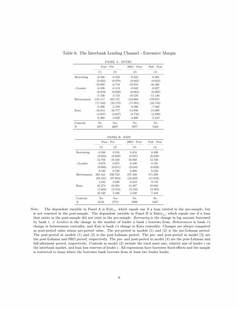
Table 6: The Interbank Lending Channel - Extensive Margin

PANEL A - ENTRY

Post - Pre SRO - Post Full - Post

(1) (2) (3) (4)

Borrowing -0.438 -0.522 -0.423 -0.365(0.032) (0.078) (0.022) (0.022)-13.680 -6.710 -18.910 -16.460

#Lender -0.108 -0.113 -0.042 -0.027(0.019) (0.030) (0.004) (0.002)-5.730 -3.710 -10.570 -11.130

Betweenness -145.117 -165.747 -153.668 -179.978(17.102) (32.173) (17.891) (23.743)-8.490 -5.150 -8.590 -7.580

Katz -16.814 -16.777 -14.880 -15.069(2.637) (4.637) (3.716) (2.890)-6.380 -3.620 -4.000 -5.210

Controls No Yes No NoN 5977 2697 5977 5568

PANEL B - EXIT

Post - Pre SRO - Post Full - Post

(1) (2) (3) (4)

Borrowing 0.506 0.516 0.454 0.498(0.034) (0.049) (0.027) (0.039)14.750 10.520 16.920 12.730

#Lender 0.078 0.075 0.108 0.191(0.008) (0.011) (0.016) (0.029)9.540 6.700 6.980 6.520

Betweenness 265.441 250.723 197.339 171.289(62.441) (87.024) (24.022) (17.633)4.250 2.880 8.210 9.710

Katz 16.274 19.294 14.287 18.056(1.608) (3.552) (3.150) (2.505)10.120 5.430 4.540 7.210

Controls No Yes No NoN 6133 2772 5898 5437

Note: The dependent variable in Panel A is Exitij , which equals one if a loan existed in the pre-sample, butis not renewed in the post-sample. The dependent variable in Panel B is Entryij , which equals one if a loanthat exists in the post-sample did not exist in the pre-sample. Borrowing is the change in log amount borrowedby bank i, # Lenders is the change in the number of lender a bank i borrows from, Betweenness is bank i’schange in betweenness centrality, and Katz is bank i’s change in Katz centrality. Changes are always computedas post-period value minus pre-period value. The pre-period in models (1) and (2) is the pre-Lehman period.The post-period in models (1) and (2) is the post-Lehman period. The pre- and post-period in model (3) arethe post-Lehman and SRO period, respectively. The pre- and post-period in model (4) are the post-Lehman andfull-allotment period, respectively. Controls in model (2) include the total asset size, relative size of lender i onthe interbank market, and loan loss reserves of lender i. All regressions have borrower fixed-effects and the sampleis restricted to loans where the borrower bank borrows from at least two lender banks.

x

Table 7: The Interbank Lending Channel - Intensive Margin, amount

Post - Pre SRO - Post Full - Post

(1) (2) (3) (4)

Borrowing 2.002 2.071 1.952 1.868(0.036) (0.052) (0.035) (0.039)56.400 39.770 56.190 48.370

#Lender 0.176 0.198 0.170 0.150(0.009) (0.019) (0.009) (0.008)19.840 10.590 18.910 18.330

Betweenness 554.159 620.073 584.355 508.034(40.168) (93.168) (40.041) (35.969)13.800 6.660 14.590 14.120

Katz 85.542 85.827 77.349 80.667(7.709) (14.377) (9.039) (6.722)11.100 5.970 8.560 12.000

Controls No Yes No NoN 6567 3070 6456 6200

Note: The dependent variable is Amountij , i.e. the change in the log of borrowing from bank i to bank j.Borrowing is the change in log amount borrowed by bank i, # Lenders is the change in the number of lender abank i borrows from, Betweenness is bank i’s change in betweenness centrality, and Katz is bank i’s change in Katzcentrality. Changes are always computed as post-period value minus pre-period value. The pre-period in models(1) and (2) is the pre-Lehman period. The post-period in models (1) and (2) is the post-Lehman period. Thepre- and post-period in model (3) are the post-Lehman and SRO period, respectively. The pre- and post-periodin model (4) are the post-Lehman and full-allotment period, respectively. Controls in model (2) include the totalasset size, relative size of lender i on the interbank market, and loan loss reserves of lender i. All regressions haveborrower fixed-effects and the sample is restricted to loans where the borrower bank borrows from at least twolender banks.

xi

Table 8: The Interbank Lending Channel - Intensive Margin, spreads

PANEL A - SPREAD

Post - Pre SRO - Post Full - Post

(1) (2) (3) (4)

Borrowing -0.009 -0.008 -0.011 -0.024(0.001) (0.002) (0.002) (0.001)-7.780 -5.430 -6.760 -16.980

#Lender -0.001 -0.001 -0.001 -0.002(0.000) (0.000) (0.000) (0.000)-4.360 -3.620 -3.860 -8.880

Betweenness -1.899 -2.231 -2.700 -6.361(0.382) (0.525) (0.805) (0.736)-4.970 -4.250 -3.350 -8.640

Katz -0.492 -0.383 -0.550 -1.243(0.065) (0.083) (0.141) (0.134)-7.590 -4.640 -3.900 -9.300

Controls No Yes No NoN 6567 3070 6456 6200

PANEL B - INTERMEDIATION SPREAD

Post - Pre SRO - Post Full - Post

(1) (2) (3) (4)

Borrowing 0.070 0.120 -0.011 0.078(0.032) (0.039) (0.002) (0.016)2.200 3.120 -6.760 5.030

#Lender 0.006 0.007 -0.001 0.006(0.002) (0.003) (0.000) (0.002)3.740 2.160 -3.860 3.370

Betweenness 23.005 27.610 -2.700 23.064(4.916) (9.741) (0.805) (5.107)4.680 2.830 -3.350 4.520

Katz 14.805 16.383 -0.550 12.138(2.305) (3.546) (0.141) (2.058)6.420 4.620 -3.900 5.900

Controls No Yes No NoN 6567 3070 6456 12400

Note: The dependent variable in Panel A is Spreadij , i.e. the volume-weighted spread bank i charges for lendingto bank j. The dependent variable in Panel B is Intermediation Spreadij , i.e. the intermediation spread bank imakes on the interbank loan to bank j. Borrowing is the change in log amount borrowed by bank i, # Lendersis the change in the number of lender a bank i borrows from, Betweenness is bank i’s change in betweennesscentrality, and Katz is bank i’s change in Katz centrality. Changes are always computed as post-period valueminus pre-period value. The pre-period in models (1) and (2) is the pre-Lehman period. The post-period inmodels (1) and (2) is the post-Lehman period. The pre- and post-period in model (3) are the post-Lehman andSRO period, respectively. The pre- and post-period in model (4) are the post-Lehman and full-allotment period,respectively. Controls in model (2) include the total asset size, relative size of lender i on the interbank market,and loan loss reserves of lender i. All regressions have borrower fixed-effects and the sample is restricted to loanswhere the borrower bank borrows from at least two lender banks.

xii

Table 9: Amount Borrowed explained by Network Centrality

Betweenness Centrality Katz Centrality

(1) (2) (3) (4) (5) (6) (7) (8)

Pre-Lehman 4.144 2.979 17.085 41.273 5.959 5.819 2.423 38.930(43.949) (43.976) (37.042) (38.677) (26.498) (26.352) (27.579) (26.330)

Post-Lehman 47.794 46.590 193.475∗∗∗ 117.080∗∗ 37.115 38.039 39.874 69.211∗

(48.461) (48.506) (56.851) (52.655) (46.934) (46.617) (48.324) (38.619)SRO -64.534 -64.337 -65.149 0.776 -7.391 -5.526 -3.518 74.618∗∗∗

(65.112) (65.010) (65.812) (60.031) (34.314) (34.151) (34.876) (23.151)Full Allotment -187.973∗∗ -187.861∗∗ -79.924 -4.739 -64.760∗ -63.485∗ -60.413 56.460∗∗

(73.647) (73.710) (62.765) (63.004) (38.551) (38.154) (39.142) (23.226)

Relative Size 268.559∗∗∗ 170.202∗∗ 216.371∗∗ -5.951 7.588∗∗ 6.759∗∗ 11.726 21.449∗∗∗

(95.026) (68.952) (100.112) (48.032) (3.827) (3.386) (8.761) (6.625)Loan Loss Reserves -0.004 -0.005 -0.063∗∗∗ -0.089∗∗∗ -0.001 0.000 -0.001 0.000

(0.004) (0.005) (0.021) (0.026) (0.001) (0.000) (0.001) (0.000)Assets 0.000 0.000 0.001∗∗∗ 0.001∗∗∗ 0.000 0.000 0.000 0.000

(0.000) (0.000) (0.000) (0.000) (0.000) (0.000) (0.000) (0.000)

Centrality 36470.5∗∗∗ 37531.0∗∗∗ 6789.673∗∗∗ 8255.118∗∗∗

(7978.657) (7172.540) (870.122) (1091.424)(Centrality × Date)Pre-Lehman -6796.209 -1147.377

(5829.444) (1260.523)Post-Lehman 9015.173∗∗ -825.757

(3642.151) (2232.239)SRO -16056.1∗∗∗ -2329.405∗

(4901.424) (1259.648)Full Allotment -19084.278∗ -3480.702∗∗∗

(10021.6) (1156.095)

Controls × date No No Yes Yes No No Yes YesN 4348 4348 4348 4348 4348 7750 4348 4348R2 (within) 0.021 0.020 0.016 0.030 0.005 0.005 0.006 0.034R2 (between) 0.000 0.304 0.159 0.520 0.003 0.594 0.004 0.601R2 (overall) 0.019 0.193 0.219 0.349 0.003 0.362 0.004 0.373

Note: Models (1) - (4) use Betweenness as Centrality, while Models (5) - (8) use Katz as Centrality. The dependentvariable is Amounti,t, i.e. the amount a bank i borrows on the interbank market on day t. The centrality of banki is computed during an initial reference period. We use the following bank-specific controls, all reported at theend of 2007: The relative size is the amount of interbank lending during the initial reference period divided bythe total asset size. The Loan Loss Reserves are a proxy for the bank’s riskiness and Assets is the total asset size.Date indicates a period dummy that is one in the respective period, and zero otherwise. The dates for the periodsare as follows. Init: 04 July - 21 July; Pre-Lehman: 28 August - 12 September; Post-Lehman: 15 September - 29September; SRO: 30 September - 14 October; Full Allotment: 15 October - 30 October.

xiii

Table 10: Borrowing Spread explained by Network Centrality

Betweenness Centrality Katz Centrality

(1) (2) (3) (4) (5) (6) (7) (8)

Pre-Lehman 0.025∗∗∗ 0.025∗∗∗ 0.024∗∗∗ 0.024∗∗∗ 0.023∗∗∗ 0.023∗∗∗ 0.024∗∗∗ 0.024∗∗∗

(0.005) (0.005) (0.006) (0.007) (0.005) (0.005) (0.006) (0.006)Post-Lehman 0.010 0.011 0.015 0.024∗ -0.005 -0.005 -0.003 -0.008

(0.011) (0.011) (0.013) (0.014) (0.009) (0.009) (0.009) (0.011)SRO -0.041 -0.041 -0.013 -0.023 -0.062∗∗∗ -0.063∗∗∗ -0.058 -0.076∗∗∗

(0.026) (0.026) (0.031) (0.034) (0.018) (0.018) (0.019) (0.020)Full Allotment -0.246∗∗∗ -0.246∗∗∗ -0.229 -0.232∗∗∗ -0.259∗∗∗ -0.259∗∗∗ -0.249 -0.270∗∗∗

(0.029) (0.029) (0.036) (0.038) (0.019) (0.019) (0.020) (0.022)

Relative Size 0.007 0.009 0.011∗ 0.017 -0.009∗ -0.009 0.010∗ 0.009(0.006) (0.006) (0.006) (0.010) (0.005) (0.005) (0.006) (0.006)

Loan Loss Reserves 0.000∗ 0.000∗∗ 0.000 0.000 0.000 0.000∗∗∗ 0.000∗∗∗ 0.000∗∗∗

(0.000) (0.000) (0.000) (0.000) (0.000) (0.000) (0.000) (0.000)Assets 0.000 0.000 0.000 0.000 0.000 0.000∗∗∗ 0.000 0.000

(0.000) (0.000) (0.000) (0.000) (0.000) (0.000) (0.000) (0.000)

Centrality -1.870 -1.848∗∗∗ 0.352∗∗∗ 0.125∗

(1.174) (0.713) (0.116) (0.066)

(Centrality × Date)Pre-Lehman 0.009 -0.010

(0.349) (0.053)Post-Lehman -1.672∗ 0.129

(0.924) (0.105)SRO 1.978 0.551∗∗

(2.409) (0.235)Full Allotment 0.611 0.603∗∗

(3.196) (0.257)

Controls × date No No Yes Yes No No Yes YesN 4348 4348 4348 4348 4348 4348 4348 4348R2 (within) 0.160 0.160 0.166 0.168 0.140 0.140 0.144 0.149R2 (between) 0.172 0.178 0.181 0.190 0.165 0.168 0.164 0.150R2 (overall) 0.131 0.134 0.140 0.145 0.121 0.127 0.123 0.132

Note: Models (1) - (4) use Betweenness as Centrality, while Models (5) - (8) use Katz as Centrality. The dependentvariable is Spreadi,t, i.e. the volume-weighted spread a bank i pays for liquidity on the interbank market on day t.The centrality of bank i is computed during an initial reference period. We use the following bank-specific controls,all reported at the end of 2007: The relative size is the amount of interbank lending during the initial referenceperiod divided by the total asset size. The Loan Loss Reserves are a proxy for the bank’s riskiness and Assets isthe total asset size. Date indicates a period dummy that is one in the respective period, and zero otherwise. Thedates for the periods are as follows. Init: 04 July - 21 July; Pre-Lehman: 28 August - 12 September; Post-Lehman:15 September - 29 September; SRO: 30 September - 14 October; Full Allotment: 15 October - 30 October.

xiv

Tab

le11:Su

mmaryStatistics

forSe

ction6

Pan

elA

–ON

Segment

Amou

nt#Le

nder

Spread

Mean

Med

ian

SDMean

Med

ian

SDMean

Med

ian

SD

Init

648.34

316

0.0

1143

.485

6.80

63.0

8.37

6-0.032

-0.014

0.15

5Pre

590.14

613

0.0

1104

.222

6.33

53.0

7.58

9-0.015

0.02

0.18

4Mon

day09

/15

659.09

215

8.5

1243

.87

7.01

84.0

8.20

90.12

30.10

20.11

Tue

sday

09/1

664

2.42

817

3.9

1044

.085

6.80

43.0

7.67

80.01

60.02

0.19

9Post

671.27

315

0.0

1178

.385

7.11

33.0

8.78

1-0.064

0.0

0.26

7SR

O570.35

516

5.0

1092

.479

6.17

43.0

7.61

5-0.076

-0.109

0.40

4Fu

ll50

5.62

515

0.0

944.40

55.08

73.0

5.76

7-0.246

-0.309

0.247

Pan

elB

–Term

Segment

Amou

nt#Le

nder

Spread

Maturity

Mean

Med

ian

SDMean

Med

ian

SDMean

Med

ian

SDMean

Med

ian

SD

Init

150.04

33.2

341.76

82.54

72.0

2.79

70.04

0.00

70.09

336

.488

19.0

50.758

Pre

132.66

630

.74

271.56

72.36

61.0

2.81

30.04

70.00

80.11

38.802

17.568

56.591

Mon

day09

/15

93.262

22.0

201.49

71.94

11.0

1.74

10.06

0.01

90.11

969

.769

30.0

90.054

Tue

sday

09/1

660

.979

30.0

85.024

2.0

1.0

1.67

50.07

10.01

40.14

339

.994

24.25

51.728

Post

85.39

25.0

166.50

52.10

61.0

2.55

40.05

70.01

0.11

430

.342

9.0

52.711

SRO

104.31

225

.039

4.38

22.01

61.0

1.84

40.10

50.034

0.16

627

.901

7.0

48.752

Full

88.516

28.5

169.04

62.00

51.0

1.82

40.06

80.00

60.13

935

.797

8.33

361

.607

Not

e:Wetake

abo

rrow

erpe

rspe

ctive,

sothat

#Len

deris

thenu

mbe

rof

lend

eraba

nkbo

rrow

sfrom

.Sp

read

ismeasuredas

thediffe

rence

ofaverageinterest

rate

tothemainrefin

ancing

rate.The

datesforthepe

riod

sareas

follo

ws.

Init:04

July

-21

July;Pre:28

Aug

ust-12

Septem

ber;

Mon

day:

15Se

ptem

ber;

Tue

sday:16

Septem

ber;

Post:

17Se

ptem

ber-29

Septem

ber;

SRO:30

Septem

ber-14

Octob

er;Fu

ll:15

Octob

er-30

Octob

er.

xv

Table 12: The Impact of the Lehman Event on Borrowers.

Panel A: Overnight Segment

Access Amount Spread Counterparties

Probit OLS OLS OLS OLS OLS OLS(1) (2) (3) (4) (5) (6) (7)

Pre-Lehman -0.063∗ -58.197 -90.941∗ 0.017∗∗ 0.023∗∗∗ -0.471 -0.749∗∗

(0.033) (50.054) (48.808) (0.007) (0.005) (0.328) (0.320)Monday 09/15 -1.546∗∗∗ 10.749 -56.962 0.155∗∗∗ 0.161∗∗∗ 0.212 -0.213

(0.048) (82.476) (79.808) (0.009) (0.008) (0.479) (0.435)Tuesday 09/16 -1.606∗∗∗ -5.915 -99.624 0.047∗∗∗ 0.053∗∗∗ -0.002 -0.774∗

(0.050) (86.159) (86.777) (0.017) (0.016) (0.469) (0.410)Post-Lehman -0.156∗∗∗ 22.931 18.294 -0.032∗∗∗ -0.028∗∗∗ 0.307 0.334

(0.033) (63.386) (63.810) (0.010) (0.010) (0.387) (0.387)SRO -0.142∗∗∗ -77.988 -149.345∗ -0.044∗∗ -0.059∗∗∗ -0.632 -1.071∗

(0.043) (75.493) (83.554) (0.021) (0.021) (0.584) (0.627)Full-allotment -0.230∗∗∗ -142.718 -270.051∗∗∗ -0.215∗∗∗ -0.223∗∗∗ -1.719∗∗∗ -2.624∗∗∗

(0.048) (88.907) (101.591) (0.022) (0.021) (0.557) (0.635)

Fixed Effects No No Yes No Yes No YesN 7, 834 6, 385 6, 385 6, 385 6, 385 6, 385 6, 385Adjusted R2 0.002 0.533 0.096 0.384 0.006 0.628

Panel B: Term Segment

Access Amount Spread Counterparties

Probit OLS OLS OLS OLS OLS OLS(1) (2) (3) (4) (5) (6) (7)

Pre-Lehman 0.042 -17.520 -17.849 0.009∗ 0.006 -0.183 -0.120(0.035) (16.341) (16.479) (0.005) (0.004) (0.119) (0.129)

Monday 09/15 -1.326∗∗∗ -56.778∗∗ -49.000∗∗ 0.031∗∗ 0.027∗ -0.606∗∗∗ -0.347∗∗

(0.062) (23.959) (24.324) (0.015) (0.016) (0.181) (0.148)Tuesday 09/16 -1.610∗∗∗ -89.061∗∗∗ -92.879∗∗∗ 0.043∗∗ 0.043∗∗ -0.547∗∗ -0.533∗∗

(0.072) (24.368) (28.155) (0.020) (0.021) (0.224) (0.239)Post-Lehman -0.209∗∗∗ -64.792∗∗∗ -69.635∗∗∗ 0.019∗∗∗ 0.018∗∗∗ -0.443∗∗ -0.418∗

(0.036) (21.292) (23.635) (0.006) (0.006) (0.187) (0.225)SRO -0.174∗∗∗ -45.204∗∗ -55.014∗∗ 0.060∗∗∗ 0.056∗∗∗ -0.530∗∗∗ -0.554∗∗

(0.041) (21.424) (25.030) (0.006) (0.006) (0.195) (0.232)Full-allotment -0.116∗∗∗ -60.446∗∗ -75.820∗∗∗ 0.029∗∗∗ 0.028∗∗∗ -0.506∗∗ -0.619∗∗∗

(0.040) (23.570) (26.890) (0.008) (0.008) (0.200) (0.225)

Fixed Effects No No Yes No Yes No YesN 5, 450 3, 646 3, 646 3, 646 3, 646 3, 646 3, 646Adjusted R2 0.007 0.162 0.030 0.236 0.006 0.331

Note: Panel A (top) shows the reaction of the overnight segment of the interbank market to the Lehman insolvency,Panel B (bottom) the reaction of the term (1d ≤ maturity ≤ 1yr) segment. The dates for the periods are asfollows. Init: 04 July - 21 July; Pre: 28 August - 12 September; Monday: 15 September; Tuesday: 16 September;Post: 17 September - 29 September; SRO: 30 September - 14 October; Full: 15 October - 30 October.

xvi

Table 13: The Impact of the Lehman Event on Lenders.

Panel A: Overnight Segment

Access Amount Spread Counterparties

Probit OLS OLS OLS OLS OLS OLS(1) (2) (3) (4) (5) (6) (7)

Pre-Lehman -0.065∗∗ -4.796 -1.885 0.084∗∗∗ 0.078∗∗∗ -0.147 -0.148(0.032) (22.871) (24.657) (0.004) (0.005) (0.131) (0.129)

Monday 09/15 -1.563∗∗∗ -8.827 -24.880 0.223∗∗∗ 0.222∗∗∗ -0.102 -0.206(0.050) (48.948) (52.237) (0.007) (0.009) (0.191) (0.202)

Tuesday 09/16 -1.660∗∗∗ -12.281 -2.338 0.049∗∗∗ 0.056∗∗∗ -0.014 -0.200(0.050) (55.425) (51.206) (0.015) (0.016) (0.187) (0.191)

Post-Lehman -0.144∗∗∗ 22.140 38.514 0.035∗∗∗ 0.040∗∗∗ 0.204 0.252(0.035) (41.777) (42.720) (0.008) (0.009) (0.171) (0.170)

SRO -0.189∗∗∗ 11.673 -9.023 -0.227∗∗∗ -0.233∗∗∗ 0.035 -0.109(0.038) (37.332) (36.659) (0.016) (0.016) (0.157) (0.159)

Full-allotment -0.179∗∗∗ -15.658 -42.869 -0.703∗∗∗ -0.707∗∗∗ -0.066 -0.219(0.040) (31.809) (37.056) (0.017) (0.017) (0.188) (0.196)

Fixed Effects No No Yes No Yes No YesN 13, 295 11, 172 11, 172 11, 172 11, 172 11, 172 11, 172Adjusted R2 −0.000 0.541 0.502 0.597 0.001 0.604

Panel B: Term Segment

Access Amount Spread Counterparties

Probit OLS OLS OLS OLS OLS OLS(1) (2) (3) (4) (5) (6) (7)

Pre-Lehman -0.041 3.949 2.339 0.026 0.038 -0.014 -0.018(0.042) (14.294) (12.705) (0.038) (0.042) (0.081) (0.086)

Monday 09/15 -1.485∗∗∗ 3.339 18.707 0.039 0.075 -0.055 -0.012(0.072) (30.052) (30.551) (0.067) (0.073) (0.184) (0.187)

Tuesday 09/16 -1.598∗∗∗ -62.604∗∗∗ -57.046∗ -0.110 -0.080 -0.284∗∗ -0.233∗

(0.077) (17.507) (29.449) (0.071) (0.075) (0.144) (0.140)Post-Lehman -0.377∗∗∗ -11.797 -1.563 -0.011 0.029 -0.144 -0.149

(0.051) (19.898) (14.231) (0.040) (0.049) (0.099) (0.104)SRO -0.289∗∗∗ 10.632 18.704 0.051 0.065 -0.182∗ -0.106

(0.050) (22.536) (21.499) (0.043) (0.047) (0.104) (0.079)Full-allotment -0.179∗∗∗ -31.793∗ 0.189 -0.405∗∗∗ -0.364∗∗∗ -0.167∗∗ -0.131∗

(0.053) (16.683) (12.205) (0.041) (0.045) (0.076) (0.078)

Fixed Effects No No Yes No Yes No YesN 5, 773 3, 279 3, 279 3, 279 3, 279 3, 279 3, 279Adjusted R2 0.002 0.344 0.069 0.188 0.002 0.183

Note: Panel A (top) shows the reaction of the overnight segment of the interbank market to the Lehman insolvency,Panel B (bottom) the reaction of the term (1d ≤ maturity ≤ 1yr) segment. The dates for the periods are asfollows. Init: 04 July - 21 July; Pre: 28 August - 12 September; Monday: 15 September; Tuesday: 16 September;Post: 17 September - 29 September; SRO: 30 September - 14 October; Full: 15 October - 30 October.

xvii

Gabrieli and Georg – "A Network View on Interbank Liquidity"

B Supplementary Information – Not for Publication

B.1 Comparison of Direct and Indirect Access to Liquidity

While we are interested in studying the effect of a bank’s network centrality on its access to liquidity,

it is instructive to compare the effect of an increase in a global measure, such as network centrality,

with the effect of an increase in local network measures, such as a bank’s weighted and unweighted

in-degree. All network variables are computed in an initial reference period to avoid issues of reverse

causality.

Tables (14) - (17) show the estimates for model 20. Banks that have 10% more lenders in the

initial period borrow on average 3.9% more subsequently and, similarly, banks that borrow a 10%

larger amount in the initial period borrow on average 2.8% more subsequently. The relation is less

pronounced for network centralities, which is to be expected as these capture also non-local effects

which can work opposite to the positive local effects.

As a robustness check, we also study access to liquidity measured as the number of coun-

terparties a bank borrows from on a given day. We use model 20 and show the results of this

estimation in Tables (18) - (21). A better network position in the initial period also translates into

access to more lenders in the subsequent periods. On aggregate the number of lenders does not

change significantly, except in the full-allotment period when it is slightly smaller than in the initial

period. Not surprising, the relative size of a bank, i.e. how much it borrows on the interbank mar-

ket in the initial period is positively correlated with the number of lenders subsequently. Our main

explanatory variables are significant again and we can observe the same pattern as with the other

measures of access to liquidity. A 10% increase in the number of lenders in the initial period leads

to a 2.6% increase in the number of lenders subsequently. A 10% increase in the amount borrowed

leads to a 1% increase in the number of subsequent borrowers. A 10% increase in betweenness

1

(Katz) centrality in the initial period leads to a 2.6% (1.2%) increase in the number of borrowers

subsequently.

Table 14: Amount Borrowed explained by In-Degree.

(1) (2) (3) (4)

Pre-Lehman 4.144 2.281 17.085 82.695∗

(43.949) (43.863) (37.042) (42.716)Post-Lehman 47.794 46.028 193.475∗∗∗ 138.676∗∗∗

(48.461) (48.557) (56.851) (52.917)SRO -64.534 -64.118 -65.149 153.333∗∗∗

(65.112) (65.235) (65.812) (53.861)Full Allotment -187.973∗∗ -187.423∗∗ -79.924 167.726∗∗

(73.647) (73.800) (62.765) (68.119)

Relative Size 268.559∗∗∗ 141.206∗∗ 216.371∗∗ -125.722∗

(95.026) (58.392) (100.112) (70.645)Loan Loss Reserves -0.004 -0.005 -0.063∗∗∗ -0.075∗∗∗

(0.004) (0.004) (0.021) (0.024)Assets 0.000 0.000 0.001∗∗∗ 0.001∗∗∗

(0.000) (0.000) (0.000) (0.000)

Degree 9.535∗∗∗ 11.090∗∗∗

(1.732) (1.676)

(Degree × Date)Pre-Lehman -2.278

(1.399)Post-Lehman 1.055

(1.428)SRO -6.855∗∗∗

(1.852)Full Allotment -8.493∗∗∗

(2.303)

Controls × date No No Yes YesN 4348 4348 4348 4348R2 (within) 0.021 0.020 0.016 0.043R2 (between) 0.000 0.355 0.159 0.549R2 (overall) 0.019 0.212 0.219 0.363

Note: The dependent variable is Amounti,t, i.e. the amount a bank i borrows on the interbank market on day t.The explanatory variable is the number of banks bank i borrows from during an initial reference period. We usethe following bank-specific controls, all reported at the end of 2007. The relative size is the amount of interbanklending during the initial reference period divided by the total asset size. The Loan Loss Reserves are a proxy forthe bank’s riskiness and Assets is the total asset size. Date indicates a period dummy that is one in the respectiveperiod, and zero otherwise. The dates for the periods are as follows. Init: 04 July - 21 July; Pre-Lehman: 28August - 12 September; Post-Lehman: 15 September - 29 September; SRO: 30 September - 14 October; FullAllotment: 15 October - 30 October.

2

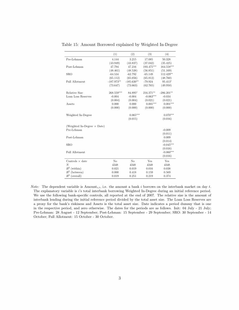
Table 15: Amount Borrowed explained by Weighted In-Degree

(1) (2) (3) (4)

Pre-Lehman 4.144 3.215 17.085 50.328(43.949) (43.837) (37.042) (35.425)

Post-Lehman 47.794 47.216 193.475∗∗∗ 164.558∗∗∗

(48.461) (48.538) (56.851) (51.169)SRO -64.534 -62.792 -65.149 112.429∗∗

(65.112) (65.056) (65.812) (48.760)Full Allotment -187.973∗∗ -185.630∗∗ -79.924 95.413∗

(73.647) (73.663) (62.765) (49.950)

Relative Size 268.559∗∗∗ 84.895∗ 216.371∗∗ -286.201∗∗

Loan Loss Reserves -0.004 -0.004 -0.063∗∗∗ -0.034(0.004) (0.004) (0.021) (0.021)

Assets 0.000 0.000 0.001∗∗∗ 0.001∗∗∗

(0.000) (0.000) (0.000) (0.000)

Weighted In-Degree 0.065∗∗∗ 0.070∗∗∗

(0.015) (0.016)

(Weighted In-Degree × Date)Pre-Lehman -0.009

(0.011)Post-Lehman 0.009

(0.014)SRO -0.045∗∗∗

(0.016)Full Allotment -0.060∗∗∗

(0.016)

Controls × date No No Yes YesN 4348 4348 4348 4348R2 (within) 0.021 0.019 0.016 0.038R2 (between) 0.000 0.418 0.159 0.569R2 (overall) 0.019 0.251 0.219 0.374

Note: The dependent variable is Amounti,t, i.e. the amount a bank i borrows on the interbank market on day t.The explanatory variable is i’s total interbank borrowing Weighted In-Degree during an initial reference period.We use the following bank-specific controls, all reported at the end of 2007. The relative size is the amount ofinterbank lending during the initial reference period divided by the total asset size. The Loan Loss Reserves area proxy for the bank’s riskiness and Assets is the total asset size. Date indicates a period dummy that is onein the respective period, and zero otherwise. The dates for the periods are as follows. Init: 04 July - 21 July;Pre-Lehman: 28 August - 12 September; Post-Lehman: 15 September - 29 September; SRO: 30 September - 14October; Full Allotment: 15 October - 30 October.

3

Table 16: Borrowing and Lending Spread explained by In-Degree.

(1) (2) (3) (4)

Pre-Lehman 0.025∗∗∗ 0.026∗∗∗ 0.024∗∗∗ 0.024∗∗∗

(0.005) (0.005) (0.006) (0.008)Post-Lehman 0.010 0.011 0.015 0.033∗∗

(0.011) (0.011) (0.013) (0.015)SRO -0.041 -0.041 -0.013 -0.001

(0.026) (0.026) (0.031) (0.036)Full Allotment -0.246∗∗∗ -0.246∗∗∗ -0.229 -0.197∗∗∗

(0.029) (0.029) (0.036) (0.043)

Relative Size 0.007 0.011∗∗ 0.011∗ 0.002(0.006) (0.006) (0.006) (0.013)

Loan Loss Reserves 0.000∗ 0.000∗∗∗ 0.000 0.000(0.000) (0.000) (0.000) (0.000)

Assets 0.000 0.000 0.000 0.000(0.000) (0.000) (0.000) (0.000)

Degree -0.001∗∗∗ 0.000(0.000) (0.000)

(Degree × Date)Pre-Lehman 0.000

(0.000)Post-Lehman -0.001∗∗∗

(0.000)SRO 0.000

(0.001)Full Allotment -0.001

(0.001)

Controls × date No No Yes YesN 4348 4348 4348 4348R2 (within) 0.160 0.160 0.166 0.170R2 (between) 0.172 0.187 0.181 0.192R2 (overall) 0.131 0.142 0.140 0.152

Note: The dependent variable is Spreadi,t, i.e. the Weighted In-Degree-weighted spread a bank i pays for liquidityon the interbank market on day t. The explanatory variable is the number of banks bank i borrows from duringan initial reference period. We use the following bank-specific controls, all reported at the end of 2007. Therelative size is the amount of interbank lending during the initial reference period divided by the total asset size.The Loan Loss Reserves are a proxy for the bank’s riskiness and Assets is the total asset size. Date indicates aperiod dummy that is one in the respective period, and zero otherwise. The dates for the periods are as follows.Init: 04 July - 21 July; Pre-Lehman: 28 August - 12 September; Post-Lehman: 15 September - 29 September;SRO: 30 September - 14 October; Full Allotment: 15 October - 30 October.

4

Table 17: Borrowing and Lending Spread explained by Weighted In-Degree

(1) (2) (3) (4)

Pre-Lehman 0.025∗∗∗ 0.025∗∗∗ 0.024∗∗∗ 0.026∗∗∗

(0.005) (0.005) (0.006) (0.007)Post-Lehman 0.010 0.011 0.015 0.027∗

(0.011) (0.011) (0.013) (0.014)SRO -0.041 -0.041 -0.013 -0.012

(0.026) (0.026) (0.031) (0.033)Full Allotment -0.246∗∗∗ -0.246∗∗∗ -0.229 -0.214∗∗∗

(0.029) (0.029) (0.036) (0.038)

Relative Size 0.007 0.011∗ 0.011∗ 0.002(0.006) (0.006) (0.006) (0.014)

Loan Loss Reserves 0.000∗ 0.000∗∗∗ 0.000 0.000(0.000) (0.000) (0.000) (0.000)

Assets 0.000 0.000 0.000 0.000(0.000) (0.000) (0.000) (0.000)

Weighted In-Degree -4.2e-06∗∗ 0.000(0.000) (0.000)

(Weighted In-Degree × Date)Pre-Lehman 0.000

(0.000)Post-Lehman -3.7e-06∗∗

(0.000)SRO 0.000

(0.000)Full Allotment 0.000

(0.000)

Controls × date No No Yes YesN 4348 4348 4348 4348R2 (within) 0.160 0.160 0.166 0.168R2 (between) 0.172 0.184 0.181 0.190R2 (overall) 0.131 0.140 0.140 0.148

Note: The dependent variable is Spreadi,t, i.e. the Weighted In-Degree-weighted spread a bank i pays for liquidityon the interbank market on day t. The explanatory variable is i’s total interbank borrowing Weighted In-Degreeduring an initial reference period. We use the following bank-specific controls, all reported at the end of 2007.The relative size is the amount of interbank lending during the initial reference period divided by the total assetsize. The Loan Loss Reserves are a proxy for the bank’s riskiness and Assets is the total asset size. Date indicatesa period dummy that is one in the respective period, and zero otherwise. The dates for the periods are as follows.Init: 04 July - 21 July; Pre-Lehman: 28 August - 12 September; Post-Lehman: 15 September - 29 September;SRO: 30 September - 14 October; Full Allotment: 15 October - 30 October.

5

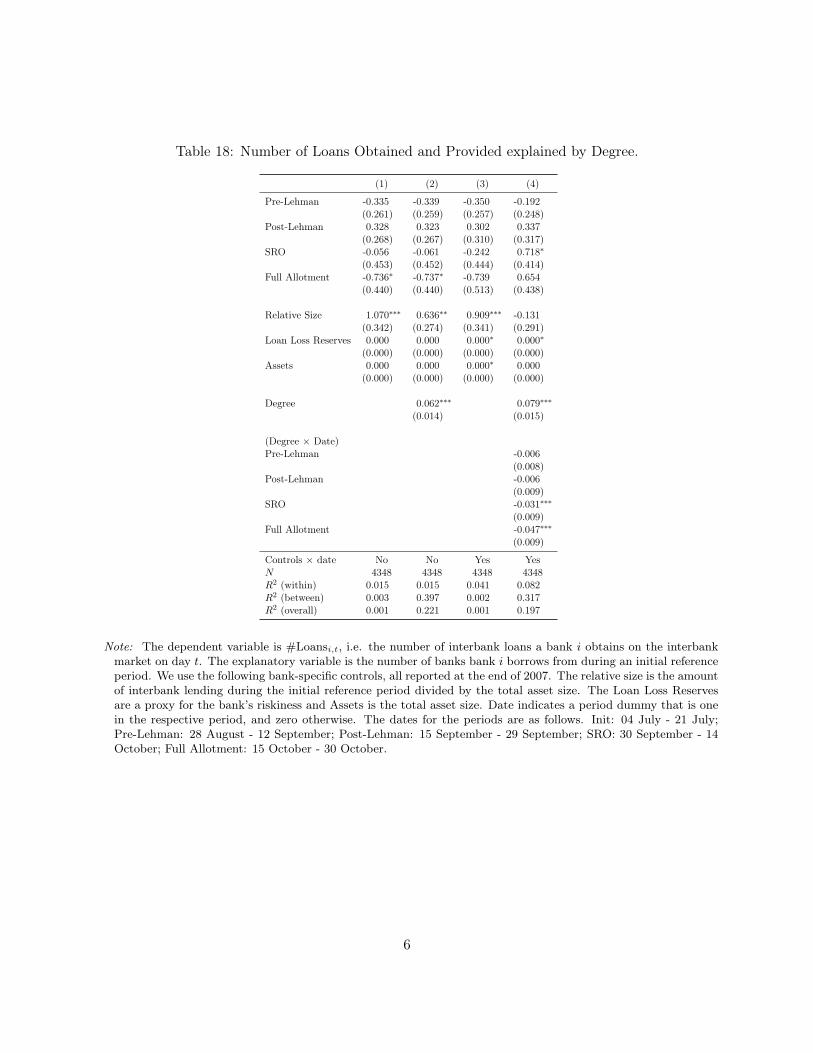
Table 18: Number of Loans Obtained and Provided explained by Degree.

(1) (2) (3) (4)

Pre-Lehman -0.335 -0.339 -0.350 -0.192(0.261) (0.259) (0.257) (0.248)

Post-Lehman 0.328 0.323 0.302 0.337(0.268) (0.267) (0.310) (0.317)

SRO -0.056 -0.061 -0.242 0.718∗

(0.453) (0.452) (0.444) (0.414)Full Allotment -0.736∗ -0.737∗ -0.739 0.654

(0.440) (0.440) (0.513) (0.438)

Relative Size 1.070∗∗∗ 0.636∗∗ 0.909∗∗∗ -0.131(0.342) (0.274) (0.341) (0.291)

Loan Loss Reserves 0.000 0.000 0.000∗ 0.000∗

(0.000) (0.000) (0.000) (0.000)Assets 0.000 0.000 0.000∗ 0.000

(0.000) (0.000) (0.000) (0.000)

Degree 0.062∗∗∗ 0.079∗∗∗

(0.014) (0.015)

(Degree × Date)Pre-Lehman -0.006

(0.008)Post-Lehman -0.006

(0.009)SRO -0.031∗∗∗

(0.009)Full Allotment -0.047∗∗∗

(0.009)

Controls × date No No Yes YesN 4348 4348 4348 4348R2 (within) 0.015 0.015 0.041 0.082R2 (between) 0.003 0.397 0.002 0.317R2 (overall) 0.001 0.221 0.001 0.197

Note: The dependent variable is #Loansi,t, i.e. the number of interbank loans a bank i obtains on the interbankmarket on day t. The explanatory variable is the number of banks bank i borrows from during an initial referenceperiod. We use the following bank-specific controls, all reported at the end of 2007. The relative size is the amountof interbank lending during the initial reference period divided by the total asset size. The Loan Loss Reservesare a proxy for the bank’s riskiness and Assets is the total asset size. Date indicates a period dummy that is onein the respective period, and zero otherwise. The dates for the periods are as follows. Init: 04 July - 21 July;Pre-Lehman: 28 August - 12 September; Post-Lehman: 15 September - 29 September; SRO: 30 September - 14October; Full Allotment: 15 October - 30 October.

6

Table 19: Number of Loans Obtained and Provided explained by Weighted In-Degree

(1) (2) (3) (4)

Pre-Lehman -0.335 -0.338 -0.350 -0.310(0.261) (0.260) (0.257) (0.244)

Post-Lehman 0.328 0.325 0.302 0.430(0.268) (0.268) (0.310) (0.297)

SRO -0.056 -0.061 -0.242 0.285(0.453) (0.453) (0.444) (0.418)

Full Allotment -0.736∗ -0.739∗ -0.739 0.016(0.440) (0.441) (0.513) (0.482)

Relative Size 1.070∗∗∗ 0.855∗∗∗ 0.909∗∗∗ -0.130(0.342) (0.305) (0.341) (0.306)

Loan Loss Reserves 0.000 0.000 0.000∗ 0.000(0.000) (0.000) (0.000) (0.000)

Assets 0.000 0.000 0.000∗ 0.000(0.000) (0.000) (0.000) (0.000)

Weighted In-Degree 0.0003∗∗∗ 0.0004∗∗∗

(0.000) (0.000)

(Weighted In-Degree × Date)Pre-Lehman 0.000

(0.000)Post-Lehman -8.5e-5∗

(0.000)SRO -0.0002∗∗∗

(0.000)Full Allotment -0.0003∗∗∗

(0.000)

Controls × date No No Yes YesN 4348 4348 4348 4348R2 (within) 0.015 0.015 0.041 0.074R2 (between) 0.003 0.165 0.002 0.091R2 (overall) 0.001 0.074 0.001 0.046

Note: The dependent variable is #Loansi,t, i.e. the number of interbank loans a bank i obtains on the interbankmarket on day t. The explanatory variable is i’s total interbank borrowing Weighted In-Degree during an initialreference period. We use the following bank-specific controls, all reported at the end of 2007. The relative size isthe amount of interbank lending during the initial reference period divided by the total asset size. The Loan LossReserves are a proxy for the bank’s riskiness and Assets is the total asset size. Date indicates a period dummythat is one in the respective period, and zero otherwise. The dates for the periods are as follows. Init: 04 July - 21July; Pre-Lehman: 28 August - 12 September; Post-Lehman: 15 September - 29 September; SRO: 30 September- 14 October; Full Allotment: 15 October - 30 October.

7

Table 20: Number of Loans Provided and Obtained explained by Betweenness Centrality

(1) (2) (3) (4)

Pre-Lehman -0.335 -0.336 -0.350 -0.313(0.261) (0.260) (0.257) (0.260)

Post-Lehman 0.328 0.327 0.302 0.165(0.268) (0.267) (0.310) (0.287)

SRO -0.056 -0.059 -0.242 0.042(0.453) (0.452) (0.444) (0.434)

Full Allotment -0.736∗ -0.737∗ -0.739 -0.350(0.440) (0.439) (0.513) (0.456)

Relative Size 1.070∗∗∗ 0.676∗∗ 0.909∗∗∗ 0.304(0.342) (0.287) (0.341) (0.285)

Loan Loss Reserves 0.000 0.000 0.000∗ -0.001∗

(0.000) (0.000) (0.000) (0.000)Assets 0.000 0.000 0.000∗ 0.000∗

(0.000) (0.000) (0.000) (0.000)

Betweenness 253.659∗∗∗ 297.845∗∗∗

(64.621) (68.367)

(Betweenness × Date)Pre-Lehman -10.101

(31.786)Post-Lehman 2.065

(27.173)SRO -65.490∗

(38.226)Full Allotment -99.634∗∗

(41.214)

Controls × date No No Yes YesN 4348 4348 4348 4348R2 (within) 0.015 0.015 0.041 0.057R2 (between) 0.003 0.389 0.002 0.323R2 (overall) 0.001 0.229 0.001 0.215

Note: The dependent variable is #Loansi,t, i.e. the number of interbank loans a bank i obtains on the interbankmarket on day t. The explanatory variable is the betweenness centrality of bank i (both perspectives) during aninitial reference period. We use the following bank-specific controls, all reported at the end of 2007. The relativesize is the amount of interbank lending during the initial reference period divided by the total asset size. TheLoan Loss Reserves are a proxy for the bank’s riskiness and Assets is the total asset size. Date indicates a perioddummy that is one in the respective period, and zero otherwise. The dates for the periods are as follows. Init: 04July - 21 July; Pre-Lehman: 28 August - 12 September; Post-Lehman: 15 September - 29 September; SRO: 30September - 14 October; Full Allotment: 15 October - 30 October.

8

Table 21: Number of Loans Obtained and Provided explained by Katz-Centrality

(1) (2) (3) (4)

Pre-Lehman -0.335 -0.339 -0.350 -0.199(0.261) (0.261) (0.257) (0.274)

Post-Lehman 0.328 0.325 0.302 0.237(0.268) (0.268) (0.310) (0.301)

SRO -0.056 -0.062 -0.242 -0.059(0.453) (0.452) (0.444) (0.439)

Full Allotment -0.736∗ -0.741∗ -0.739 -0.686(0.440) (0.440) (0.513) (0.509)

Relative Size 1.070∗∗∗ 1.063∗∗∗ 0.909∗∗∗ 0.850∗∗∗

(0.342) (0.333) (0.341) (0.330)Loan Loss Reserves 0.000 0.000 0.000∗ 0.000∗

(0.000) (0.000) (0.000) (0.000)Assets 0.000 0.000 0.000∗ 0.000

(0.000) (0.000) (0.000) (0.000)

Katz 15.970∗∗∗ 16.394∗∗

(4.848) (7.580)

(Katz × Date)Pre-Lehman -7.322

(5.495)Post-Lehman -0.103

(5.216)SRO -7.751

(7.388)Full Allotment -3.037

(7.168)

Controls × date No No Yes YesN 4348 4348 4348 4348R2 (within) 0.015 0.015 0.041 0.045R2 (between) 0.003 0.048 0.002 0.013R2 (overall) 0.001 0.016 0.001 0.003

Note: The dependent variable is #Loansi,t, i.e. the number of interbank loans a bank i obtains on the interbankmarket on day t. The explanatory variable is the Katz centrality of bank i (both perspectives) during an initialreference period. We use the following bank-specific controls, all reported at the end of 2007. The relative size isthe amount of interbank lending during the initial reference period divided by the total asset size. The Loan LossReserves are a proxy for the bank’s riskiness and Assets is the total asset size. Date indicates a period dummythat is one in the respective period, and zero otherwise. The dates for the periods are as follows. Init: 04 July - 21July; Pre-Lehman: 28 August - 12 September; Post-Lehman: 15 September - 29 September; SRO: 30 September- 14 October; Full Allotment: 15 October - 30 October.

9

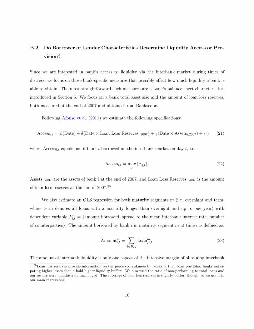
B.2 Do Borrower or Lender Characteristics Determine Liquidity Access or Pro-

vision?

Since we are interested in bank’s access to liquidity via the interbank market during times of

distress, we focus on those bank-specific measures that possibly affect how much liquidity a bank is

able to obtain. The most straightforward such measures are a bank’s balance sheet characteristics,

introduced in Section 5. We focus on a bank total asset size and the amount of loan loss reserves,

both measured at the end of 2007 and obtained from Bankscope.

Following Afonso et al. (2011) we estimate the following specifications:

Accessi,t = β(Date) + δ(Date× Loan Loss Reservesi,2007) + γ(Date×Assetsi,2007) + εi,t (21)

where Accessi,t equals one if bank i borrowed on the interbank market on day t, i.e.:

Accessi,t = maxj{gij,t}. (22)

Assetsi,2007 are the assets of bank i at the end of 2007, and Loan Loss Reservesi,2007 is the amount

of loan loss reserves at the end of 2007.25

We also estimate an OLS regression for both maturity segments m (i.e. overnight and term,

where term denotes all loans with a maturity longer than overnight and up to one year) with

dependent variable Fmi,t = {amount borrowed, spread to the mean interbank interest rate, number

of counterparties}. The amount borrowed by bank i in maturity segment m at time t is defined as:

Amountmi,t =∑j∈Bi,t

Loanmji,t. (23)

The amount of interbank liquidity is only one aspect of the intensive margin of obtaining interbank25Loan loss reserves provide information on the perceived riskiness by banks of their loan portfolio: banks antici-

pating higher losses should hold higher liquidity buffers. We also used the ratio of non-performing to total loans andour results were qualitatively unchanged. The coverage of loan loss reserves is slightly better, though, so we use it inour main regressions.

10

liquidity. The other aspect is the price a bank pays for liquidity, measured as the spread to the main

refinancing rate (in the overnight segment) or the average interbank interest rate (for the maturity

segments). For each point in time t and each maturity segment we have a network Gmt . Denote

the price of a loan from i to j at time t with maturity m as pmij,t and the volume-weighted price in

maturity segment m as p̂mij,t. Then:

p̂mij,t = pmij,t ×Loanmij,t∑

j∈Bi,t Loanmij,t

. (24)

The spread to the mean interbank interest rate that borrower i pays on the interbank market at

time t in maturity m is defined as:

Spreadm,bi,t =∑j∈Bi,t

p̂mij,t − p̂mt . (25)

where p̂mt is the average interbank interest rate in maturity segmentm at time t, p̂mt =

∑i

∑j:i p̂

mij,t.26

Using these definitions, we can specify OLS estimations that take borrower properties into

account as:

Fi,t = β(Date) + δ(Date× Loan Loss Reservesi,2007) + γ(Date×Assetsi,2007) (26)

+Θ

(Amounti,tAssetsi,2007

)+ αi + εi,t

where Amounti,t is the amount borrowed by bank i in both maturity segments and αi are bank fixed

effects. As before, the sample period runs from 04 July 2008 to 30 October 2008. In Tables (22)

to (25) we split our sample in two subsamples based on banks’ asset size. Large banks are in the

upper tercile of the asset size distribution, while small banks are in the lower tercile. Furthermore,

interacting the period dummies with borrower quality, measured by a bank i’s loan loss reserves

yields a triple difference-in-difference estimation that tests whether the interbank market has become26The computation for the average interest rate was done in three maturity segment separately to ensure comparable

results across maturities. Loans in the three segments have maturity m with: 1day < m ≤ 1week ; 1week < m ≤3month ; 3month < m < 1year.Differently from the term maturities, the spread for the overnight maturity is definedrelative to the main refinancing rate.

11

sensitive to bank characteristics post-crisis and whether the sensitivity is greater for large or small

banks.

As pointed out by Afonso et al. (2011), if lenders respond to the crisis by hoarding liquidity,

we would expect to find an aggregate decrease in amounts lent and worse performing banks lending

less. If instead uncertainty about counterparty risk increases after a shock but banks can still

discriminate between risks, then we would expect to find a large shift in the distribution of funds

and rates in the cross section of borrowers and worse performing banks borrowing less and/or

paying higher rates. The aggregate view of market developments taken so far allows us to exclude

an aggregate decrease in amounts lent after the bankruptcy of Lehman (with the only exception of

the reduction on Tuesday 09/16 in the term segment). Moreover, in Table 12 we saw that bank-

specific characteristics drove a relatively high increase in overnight and term borrowing rates and a

reduction in the number of counterparties from which banks could obtain liquidity. Only in the term

segment these developments are associated to a generalized decrease in borrowed amounts. This

overall picture seems consistent with an increase in counterparty risk in the euro area interbank

market around the Lehman event, especially in the ovenight segment, and a more pronounced

market freeze only in the term segment.

Tables (22) and (23) corroborate and shed further light on this picture. Access to the market

is reduced on Monday 15 and Tuesday 16, and especially so for small borrowers and for the overnight

segment (models (1) and (2)). In models (3) and (4) we add interactions of the period dummies with

loan loss reserves as a proxy for borrower quality. The interaction terms reveal that large borrowers

whose loan portfolio is riskier pre-crisis access the overnight market less, both around the Lehman

event and afterwards. No such effect is visible for small borrowers. In contrast, in the term segment

large, worse performing borrowers are found to actually increase their participation pre-Lehman

and especially on Tuesday 16 September (model (7)). Evidence from Table (23) confirms that there

was no decrease in amounts borrowed overnight around Lehman, not even for the worse performing

banks. The significant and large coefficient on the large banks for the full-allotment period in

model (3) tells us that it was large borrowers who strongly reduced their interbank funding after

12

the Eurosystem switched to full-allotment operations in mid-October 2008. It were small banks

that reduced their interbank funding in the term segment on Monday 15 September and in the

full-allotment regime, instead.

Table (24) shows that both large and small banks see an increase in overnight spreads on

Monday 15 September. However, the increase persists only for small banks on Tuesday 16 Septem-

ber, while large banks actually start borrowing at a discount, relative to the initial reference period,

both in the post-Lehman period and especially after the ECB measures (SRO and full-allotment).

When we add interactions of the period dummies with loan loss reserves, models (3) and (4), we

still observe the increase in spreads on Monday 15 September (larger for small banks), but we do

not see a significant deterioration of borrowing terms for small worse performing banks immediately

after the Lehman event. The only significant and positive coefficient appears for the interaction

between loan loss reserves and the SRO period dummy, which suggests that small banks with a

riskier loan portfolio pre-crisis could not obtain all the liquidity they needed at the Eurosystem’s

special refinancing operation. For the term segment, models (5) to (8) show that immediately after

the crisis the relationship between spreads and borrower quality was not significantly different from

that for the pre-crisis period, i.e. interest rates in the term segment did not become increasingly

sensitive to measures of borrower quality.

We find similar evidence in Table (25) for the number of counterparties a bank borrows from.

The results do not provide strong evidence of a changed market sensitivity of to borrower size, nor to

borrower quality immediately after the Lehman insolvency. The only significant and economically

sizeable effect can be observed after the adoption of the full-allotment regime on 15 October, when

large banks reduce the number of counterparties from which they borrow (−2.6 counterparties in

model (1) and −3.4 in model (3)). A similar effect is found in the term segment, again for large

banks, but this effect is not as large as in the overnight segment.

Overall, these tables do not show a drastic change in the distribution of loans and rates in

the cross section of borrowers depending on borrower pre-crisis quality, at least not immediately

after the Lehman insolvency. This does not mean, however, that the market was not sensitive to

13

counterparty risks, as we have shown in the aggregate perspective in Table (12). In a situation

of stress, lenders may rather start to manage their unsecured interbank exposures by the amount

they lend to a particular bank or even whether they lend to a given bank at all. Bank-to-bank

relationships may actually become more important for the lenders’ decision because they convey

soft information that cannot be otherwide obtained from pre-crisis balance sheets. But this means

that a more granular analysis of bilateral links between banks is needed. This motivates our network

view in the rest of the paper.

14

Tab

le22

:Im

pact

ofLe

hman

Event

onBorrower

Access

Overnight

Term

Large

Small

Large

Small

Large

Small

Large

Small

(1)

(2)

(3)

(4)

(5)

(6)

(7)

(8)

Pre-Leh

man

-0.107

-0.125∗

-0.193∗∗

-0.141

0.04

10.09

00.13

10.06

2(0.066

)(0.073

)(0.084

)(0.134

)(0.071

)(0.074

)(0.082

)(0.105

)Mon

day09

/15

-1.332∗∗∗

-1.678∗∗∗

-1.393∗∗∗

-1.569∗∗∗

-1.226∗∗∗

-1.401∗∗∗

-1.078∗∗∗

-1.342∗∗∗

(0.112

)(0.098

)(0.131

)(0.154

)(0.129

)(0.121

)(0.174

)(0.173

)Tue

sday

09/1

6-1.409∗∗∗

-1.760∗∗∗

-1.484∗∗∗

-1.784∗∗∗

-1.669∗∗∗

-1.639∗∗∗

-1.437∗∗∗

-1.462∗∗∗

(0.120

)(0.088

)(0.139

)(0.144

)(0.117

)(0.154

)(0.149

)(0.211

)Post-Le

hman

-0.145∗

-0.171∗∗

-0.283∗∗∗

-0.127

-0.182∗∗∗

-0.156∗∗

-0.251∗∗∗

-0.089

(0.080

)(0.071

)(0.094

)(0.126

)(0.065

)(0.075

)(0.072

)(0.102

)SR

O-0.055

-0.176∗∗

-0.141

-0.108

-0.174∗∗

-0.106

-0.181

0.00

2(0.097

)(0.088

)(0.115

)(0.139

)(0.080

)(0.081

)(0.114

)(0.117

)Fu

ll-allotm

ent

-0.239∗∗

-0.275∗∗∗

-0.336∗∗∗

-0.237

-0.060

-0.166∗

-0.073

-0.188

(0.106

)(0.096

)(0.128

)(0.162

)(0.083

)(0.093

)(0.114

)(0.134

)

Pre-Leh

man×Lo

anLo

ssReserves

-0.000

01∗∗

-0.001

0.00

002∗∗∗

0.00

1(0.000

)(0.001

)(0.000

)(0.001

)Mon

day09

/15×

Loan

Loss

Reserves

-0.000

04∗

-0.003

0.00

00.00

3(0.000

)(0.002

)(0.000

)(0.002

)Tue

sday

09/1

6×Lo

anLo

ssReserves

-0.000

04∗∗

-0.002

0.00

005∗∗∗

-0.001

(0.000

)(0.002

)(0.000

)(0.002

)Post-Le

hman×Lo

anLo

ssReserves

-0.000

01∗∗∗

-0.001

0.00

0-0.001

(0.000

)(0.001

)(0.000

)(0.001

)SR

O×Lo

anLo

ssReserves

-0.000

01∗∗

-0.001

-0.000

0.00

1(0.000

)(0.001

)(0.000

)(0.001

)Fu

ll-allotm

ent×

Loan

Loss

Reserves

-0.000

01∗∗∗

-0.001

0.00

0-0.000

(0.000

)(0.002

)(0.000

)(0.001

)

Fixed

Effe

cts

No

No

No

No

No

No

No

No

N2,6

172,6

182,6

172,6

181,8

28

1,8

38

1,8

28

1,8

38

Not

e:Im

pact

oftheLeh

man

eventon

borrow

ers.

Term

segm

entinclud

esallloans

withamaturityof

long

erthan

oneda

yan

dup

toon

eyear.

Large

(small)

bank

sarein

theup

per(low

er)tercile

ofAssets 2

007.The

datesforthepe

riod

sareas

follo

ws.

Init:04

July

-21

July;Pre:

28Aug

ust-12

Septem

ber;

Mon

day:

15Se

ptem

ber;

Tue

sday:16

Septem

ber;

Post:

17Se

ptem

ber-29

Septem

ber;

SRO:30

Septem

ber-14

Octob

er;F

ull:

15Octob

er-30

Octob

er.

15

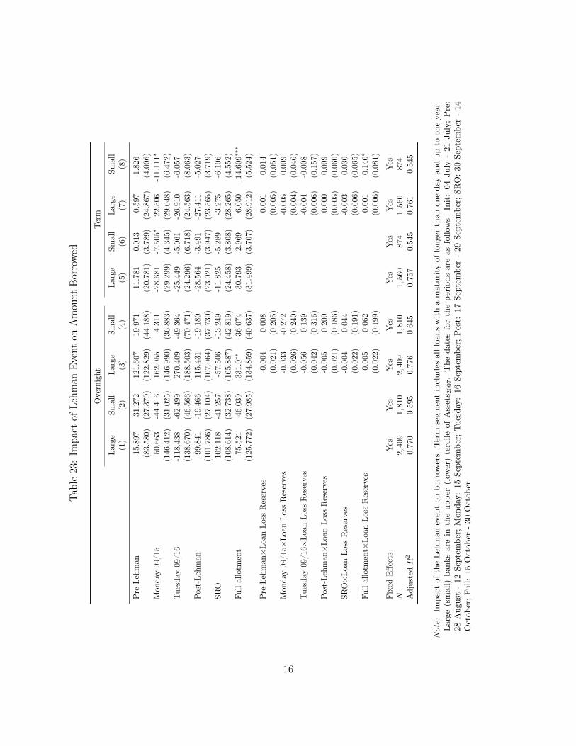
Tab

le23:Im

pact

ofLe

hman

Event

onAmou

ntBorrowed

Overnight

Term

Large

Small

Large

Small

Large

Small

Large

Small

(1)

(2)

(3)

(4)

(5)

(6)

(7)

(8)

Pre-Leh

man

-15.89

7-31.27

2-121

.607

-19.97

1-11.781

0.01

30.59

7-1.826

(83.58

0)(27.37

9)(122

.829

)(44.188)

(20.78

1)(3.789

)(24.86

7)(4.006

)Mon

day09

/15

50.663

-44.41

616

2.05

54.311

-28.68

1-7.505∗

22.506

-11.11

1∗

(146

.412

)(31.02

5)(146

.990

)(36.883)

(29.29

9)(4.345

)(29.04

8)(6.472

)Tue

sday

09/1

6-118.438

-62.49

927

0.40

9-49.36

4-25.44

9-5.061

-26.91

0-6.057

(138

.670

)(46.56

6)(188

.503

)(70.471)

(24.29

6)(6.718

)(24.56

3)(8.063

)Post-Le

hman

99.841

-19.46

611

5.43

1-19.18

0-28.56

4-3.491

-27.41

1-5.027

(101

.786

)(27.10

4)(107

.064

)(37.730)

(23.02

1)(3.947

)(23.56

5)(3.719

)SR

O10

2.11

8-41.257

-57.50

6-13.24

9-11.82

5-5.289

-3.275

-6.106

(108

.614

)(32.73

8)(105

.887

)(42.819)

(24.45

8)(3.808

)(28.26

5)(4.552

)Fu

ll-allotm

ent

-75.521

-46.03

9-331

.0∗∗

-36.07

4-30.79

3-2.969

-6.050

-14.60

9∗∗∗

(125

.772

)(27.98

5)(134

.859

)(40.637)

(31.49

9)(3.707

)(28.91

2)(5.524

)

Pre-Leh

man×Lo

anLo

ssReserves

-0.004

0.00

80.00

10.01

4(0.021

)(0.205

)(0.005

)(0.051

)Mon

day09

/15×

Loan

Loss

Reserves

-0.033

-0.272

-0.005

0.00

9(0.026

)(0.240

)(0.004

)(0.046

)Tue

sday

09/1

6×Lo

anLo

ssReserves

-0.056

0.13

9-0.004

-0.008

(0.042

)(0.316

)(0.006

)(0.157

)Post-Le

hman×Lo

anLo

ssReserves

-0.005

0.20

00.00

00.009

(0.021

)(0.186

)(0.005

)(0.060

)SR

O×Lo

anLo

ssReserves

-0.004

0.04

4-0.003

0.03

0(0.022

)(0.191

)(0.006

)(0.065

)Fu

ll-allotm

ent×

Loan

Loss

Reserves

-0.005

0.06

20.00

10.14

0∗

(0.022

)(0.199

)(0.006

)(0.081

)

Fixed

Effe

cts

Yes

Yes

Yes

Yes

Yes

Yes

Yes

Yes

N2,

409

1,81

02,

409

1,81

01,5

60874

1,56

087

4AdjustedR

20.7

700.5

950.7

760.6

450.

757

0.54

50.

761

0.54

5

Not

e:Im

pact

oftheLeh

man

eventon

borrow

ers.

Term

segm

entinclud

esallloans

withamaturityof

long

erthan

oneda

yan

dup

toon

eyear.

Large

(small)

bank

sarein

theup

per(low

er)tercile

ofAssets 2

007.The

datesforthepe

riod

sareas

follo

ws.

Init:04

July

-21

July;Pre:

28Aug

ust-12

Septem

ber;

Mon

day:

15Se

ptem

ber;

Tue

sday:16

Septem

ber;

Post:

17Se

ptem

ber-29

Septem

ber;

SRO:30

Septem

ber-14

Octob

er;F

ull:

15Octob

er-30

Octob

er.

16

Tab

le24:Im

pact

ofLe

hman

Event

onSp

read

s

Overnight

Term

Large

Small

Large

Small

Large

Small

Large

Small

(1)

(2)

(3)

(4)

(5)

(6)

(7)

(8)

Pre-Leh

man

0.02

4∗∗∗

0.02

0∗-0.000

0.04

9∗∗

0.00

60.00

60.01

10.00

6(0.008

)(0.012

)(0.020

)(0.021

)(0.008)

(0.007

)(0.011

)(0.013

)Mon

day09

/15

0.15

7∗∗∗

0.15

8∗∗∗

0.14

2∗∗∗

0.16

5∗∗∗

0.00

50.06

40.00

80.09

2(0.011

)(0.021

)(0.026

)(0.037

)(0.011)

(0.056

)(0.015

)(0.095

)Tue

sday

09/1

6-0.021

0.13

3∗∗∗

-0.007

0.12

5∗∗∗

0.04

10.02

60.08

30.03

5(0.026

)(0.026

)(0.035

)(0.045

)(0.031)

(0.017

)(0.062

)(0.028

)Post-Le

hman

-0.076∗∗∗

0.02

5-0.123∗∗∗

0.01

80.01

7∗∗

0.03

0∗∗

0.03

0∗0.00

9(0.017

)(0.017

)(0.027

)(0.029

)(0.008)

(0.013

)(0.011

)(0.014

)SR

O-0.132∗∗∗

0.06

1-0.224∗∗∗

-0.006

0.05

2∗∗∗

0.06

1∗∗∗

0.05

6∗∗∗

0.07

0∗∗∗

(0.031

)(0.039

)(0.035

)(0.062

)(0.009)

(0.012

)(0.012

)(0.019

)Fu

ll-allotm

ent

-0.296∗∗∗

-0.126∗∗∗

-0.358∗∗∗

-0.119

0.03

1∗∗

0.01

10.04

2∗∗

-0.000

(0.020

)(0.043

)(0.026

)(0.083

)(0.013)

(0.010

)(0.016

)(0.013

)

Pre-Leh

man×Lo

anLo

ssReserves

0.00

0-0.000

3∗∗

-0.000

-0.000

(0.000

)(0.000

)(0.000

)(0.000

)Mon

day09

/15×

Loan

Loss

Reserves

0.00

00.00

0-0.000

-0.000

(0.000

)(0.000

)(0.000

)(0.000

)Tue

sday

09/1

6×Lo

anLo

ssReserves

-0.000

0.00

0-0.000

005∗

-0.000

(0.000

)(0.000

)(0.000

)(0.000

)Post-Le

hman×Lo

anLo

ssReserves

0.00

00.00

0-0.000

001∗

0.00

0(0.000

)(0.000

)(0.000

)(0.000

)SR

O×Lo

anLo

ssReserves

0.00

00.00

1∗∗

-0.000

-0.000

(0.000

)(0.000

)(0.000

)(0.000

)Fu

ll-allotm

ent×

Loan

Loss

Reserves

0.00

0-0.000

-0.000

02∗∗∗

0.00

0(0.000

)(0.001

)(0.000

)(0.000

)

Fixed

Effe

cts

Yes

Yes

Yes

Yes

Yes

Yes

Yes

Yes

N2,

409

1,8

102,4

091,

810

1,56

087

41,5

60874

AdjustedR

20.

333

0.48

00.

346

0.4

880.2

070.

410

0.2

060.4

18

Not

e:Im

pact

oftheLeh

man

eventon

borrow

ers.

Term

segm

entinclud

esallloans

withamaturityof

long

erthan

oneda

yan

dup

toon

eyear.

Large

(small)

bank

sarein

theup

per(low

er)tercile

ofAssets 2

007.The

datesforthepe

riod

sareas

follo

ws.

Init:04

July

-21

July;Pre:

28Aug

ust-12

Septem

ber;

Mon

day:

15Se

ptem

ber;

Tue

sday:16

Septem

ber;

Post:

17Se

ptem

ber-29

Septem

ber;

SRO:30

Septem

ber-14

Octob

er;F

ull:

15Octob

er-30

Octob

er.

17

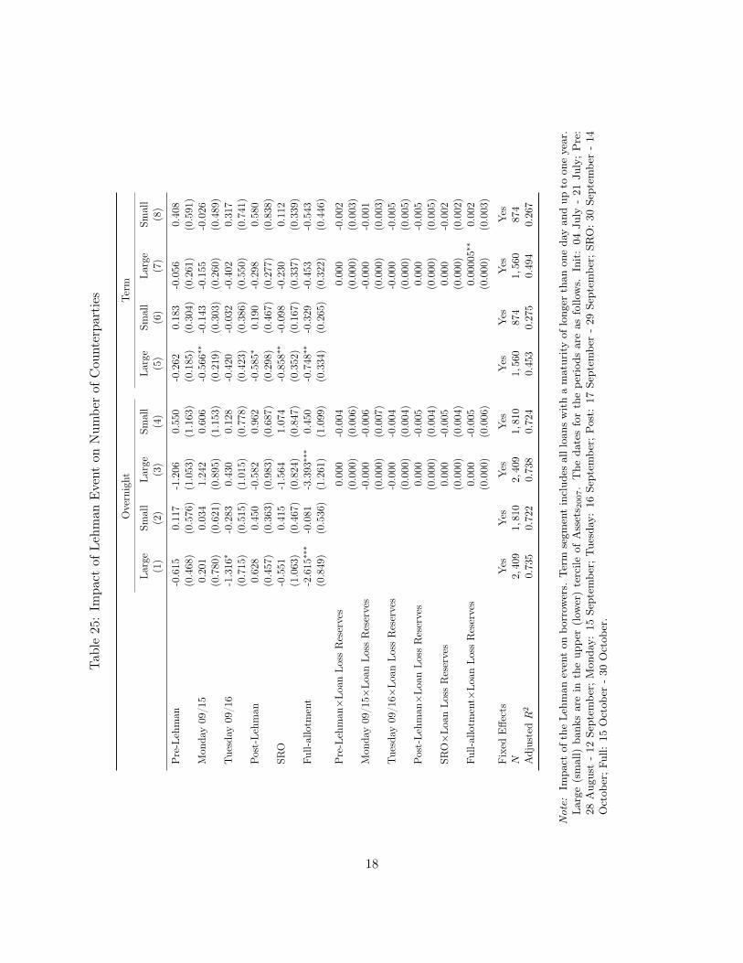
Tab

le25

:Im

pact

ofLe

hman

Event

onNum

berof

Cou

nterpa

rties

Overnight

Term

Large

Small

Large

Small

Large

Small

Large

Small

(1)

(2)

(3)

(4)

(5)

(6)

(7)

(8)

Pre-Leh

man

-0.615

0.11

7-1.206

0.55

0-0.262

0.18

3-0.056

0.40

8(0.468

)(0.576

)(1.053

)(1.163

)(0.185

)(0.304

)(0.261

)(0.591

)Mon

day09

/15

0.20

10.03

41.24

20.606

-0.566∗∗

-0.143

-0.155

-0.026

(0.780

)(0.621

)(0.895

)(1.153

)(0.219

)(0.303

)(0.260

)(0.489

)Tue

sday

09/1

6-1.316∗

-0.283

0.43

00.12

8-0.420

-0.032

-0.402

0.31

7(0.715

)(0.515

)(1.015

)(0.778

)(0.423

)(0.386

)(0.550

)(0.741

)Post-Le

hman

0.62

80.45

0-0.582

0.96

2-0.585∗

0.19

0-0.298

0.58

0(0.457

)(0.363

)(0.983

)(0.687

)(0.298

)(0.467

)(0.277

)(0.838

)SR

O-0.551

0.41

5-1.564

1.07

4-0.858∗∗

-0.098

-0.230

0.11

2(1.063

)(0.467

)(0.824

)(0.847

)(0.352

)(0.167

)(0.337

)(0.339

)Fu

ll-allotm

ent

-2.615∗∗∗

-0.081

-3.393∗∗∗

0.45

0-0.748∗∗

-0.329

-0.453

-0.543

(0.849

)(0.536

)(1.261

)(1.099

)(0.334

)(0.265

)(0.322

)(0.446

)

Pre-Leh

man×Lo

anLo

ssReserves

0.000

-0.004

0.00

0-0.002

(0.000

)(0.006

)(0.000

)(0.003

)Mon

day09

/15×

Loan

Loss

Reserves

-0.000

-0.006

-0.000

-0.001

(0.000

)(0.007

)(0.000

)(0.003

)Tue

sday

09/1

6×Lo

anLo

ssReserves

-0.000

-0.004

-0.000

-0.005

(0.000

)(0.004

)(0.000

)(0.005

)Post-Le

hman×Lo

anLo

ssReserves

0.00

0-0.005

0.00

0-0.005

(0.000

)(0.004

)(0.000

)(0.005

)SR

O×Lo

anLo

ssReserves

0.00

0-0.005

0.00

0-0.002

(0.000

)(0.004

)(0.000

)(0.002

)Fu

ll-allotm

ent×

Loan

Loss

Reserves

0.00

0-0.005

0.00

005∗∗

0.00

2(0.000

)(0.006

)(0.000

)(0.003

)

Fixed

Effe

cts

Yes

Yes

Yes

Yes

Yes

Yes

Yes

Yes

N2,4

091,

810

2,40

91,

810

1,5

6087

41,

560

874

AdjustedR

20.7

350.7

220.7

380.7

240.4

530.2

750.4

940.2

67

Not

e:Im

pact

oftheLeh

man

eventon

borrow

ers.

Term

segm

entinclud

esallloans

withamaturityof

long

erthan

oneda

yan

dup

toon

eyear.

Large

(small)

bank

sarein

theup

per(low

er)tercile

ofAssets 2

007.The

datesforthepe

riod

sareas

follo

ws.

Init:04

July

-21

July;Pre:

28Aug

ust-12

Septem

ber;

Mon

day:

15Se

ptem

ber;

Tue

sday:16

Septem

ber;

Post:

17Se

ptem

ber-29

Septem

ber;

SRO:30

Septem

ber-14

Octob

er;F

ull:

15Octob

er-30

Octob

er.

18

B.3 Can Nodes Influence their own Centrality?

In Khwaja and Mian (2008) banks experience an exogenous liquidity shock due to sanctions imposed

on Pakistan following an unannounced nuclear weapon’s test. This exogenous shock is crucial for

identification and begs the question whether a change in a node’s network centrality can be seen as

exogenous. We use three shocks in this paper: the insolvency of the US investment bank Lehman

Brothers on 15 September 2008 (our main specification), the first full-allotment special refinancing

operation on 29 September, and the decision by the Eurosystem to move from a variable-rate

auction-based regime of monetary policy to a full-allotment regime on 15 October 2008. Our main

hypothesis is that banks in a more central position within the network have easier access to more and

cheaper liquidity. We show in Section 2 that the interbank network structure changes significantly

between the different sample periods. This aggregate change causes substantial change in individual

banks’ network position (measured by their degree, volume, and centralities). We test the hypothesis

that this change in bank i’s network position leads to a change in i’s liquidity provision and access

using a diff-in-diff setting similar to Khwaja and Mian (2008).

However, one concern could be that banks can strategically choose their network position. A

change in their network position would thus not be an exogenous shock. In this section we thus

test whether banks can indeed strategically choose a certain value of their centrality. Intuitively, we

expect this not to be the case because a bank’s centrality depends on the entire network structure,

while the bank can only decide about its immediate neighborhood (i.e. whether to form a link with

other banks and thus add them to the neighborhood). While there is no easy analytical proof of

our intuition, we can test it numerically.

Consider the following simple algorithm with seven steps:

1. Select an undirected random network with N nodes. Since interbank networks are typically

of core-periphery type, we draw NG core-periphery networks G with N nodes. 27.27In line with the evidence commonly found in the empirical literature on interbank networks, we set the number

of cores for each network randomization to be chosen randomly between 10− 20% of the total number of nodes

19

2. Select Nr random reference nodes r.

3. Calculate the initial centrality of the reference node Cir where C ∈ {Betweenness,Katz}.

4. Add Nm random links to/from the reference node r.

5. Allow the rest of the network to change: select N−r random nodes in the network and change

a random number of links of these, that are not to/from the reference node r.

6. Now calculate the updated centrality of the reference node Cur and compute the absolute

change in the centrality (relative to the initial centrality):

∆Cr =

∣∣∣∣Cur − CirCir

∣∣∣∣ .7. Calculate the mean of ∆Cr.28.

We perform the numerical simulation both for core-periphery network configuration and for

Erdös-Rényi network with rewiring probability equal to 0.8. Choosing a high value for the last

parameter, we aim to reflect the empirical evidence that interbank market structure is relatively

tightly knit. As it has been argued by Haldane (2009) indeed, the financial sector has undergone

increasing levels of homogeneity. Moreover, several empirical papers show that bank networks

feature a core-periphery structure with a core of big and densely connected banks and a periphery

of smaller banks. Our hypothesis aims therefore to capture the opportunity for banks in this core

to change their network position.

In Figure 5 we show the change in the centrality measures of node r in a log scale and do

linear fit, which corresponds to an exponential increase in the mean of ∆Cr. We obtain in general

a good level of the linear fit of the two series in log scale, as shown by the R-square values of

0.92 and 0.72 calculated respectively for the core-periphery and the Erdös-Rényi network. This28Technically, in the numerical simulation we compute three averages. First, we calculate the average change in the

reference node centrality induced by othersâĂŹ links change over Nm different links randomizations of the referencenode r. The calculation of this average is performed for Nr random reference nodes selected (using the same initialnetwork configuration selected in step 1.) and the mean of these averages is calculated over NG random configurationsof the network. This last average gives the value for ∆Cr for each given number of nodes.

20

implies that increasing network size, the change in a node r’s centrality due to changes outside

of the neighborhood of r increases more than the change in r’s centrality due to changes in the

neighborhood of r. Accordingly, the results of the analysis support our intuition that nodes cannot

influence their centrality and strategically choose their network position.

21

Figure 5: Mean relative change ∆Cr in node r’s centrality versus network size. Mean is computedover NG = 100 random draws, Nr = 10 random reference nodes that can randomly change Nm = 10links, and N−r = 1 random changes of links outside r’s neighborhood. We use core-peripherynetwork (top) and Erdös-Rényi network with rewiring probability equal to 0.8 (bottom).

22