A Neural Network Truth Maintenance System

Louisiana State UniversityLSU Digital Commons

LSU Historical Dissertations and Theses Graduate School

1991

A Neural Network Truth Maintenance System.Suresh GuddantiLouisiana State University and Agricultural & Mechanical College

Follow this and additional works at: https://digitalcommons.lsu.edu/gradschool_disstheses

This Dissertation is brought to you for free and open access by the Graduate School at LSU Digital Commons. It has been accepted for inclusion inLSU Historical Dissertations and Theses by an authorized administrator of LSU Digital Commons. For more information, please [email protected].

Recommended CitationGuddanti, Suresh, "A Neural Network Truth Maintenance System." (1991). LSU Historical Dissertations and Theses. 5185.https://digitalcommons.lsu.edu/gradschool_disstheses/5185

https://digitalcommons.lsu.edu?utm_source=digitalcommons.lsu.edu%2Fgradschool_disstheses%2F5185&utm_medium=PDF&utm_campaign=PDFCoverPages

https://digitalcommons.lsu.edu/gradschool_disstheses?utm_source=digitalcommons.lsu.edu%2Fgradschool_disstheses%2F5185&utm_medium=PDF&utm_campaign=PDFCoverPages

https://digitalcommons.lsu.edu/gradschool?utm_source=digitalcommons.lsu.edu%2Fgradschool_disstheses%2F5185&utm_medium=PDF&utm_campaign=PDFCoverPages

https://digitalcommons.lsu.edu/gradschool_disstheses?utm_source=digitalcommons.lsu.edu%2Fgradschool_disstheses%2F5185&utm_medium=PDF&utm_campaign=PDFCoverPages

https://digitalcommons.lsu.edu/gradschool_disstheses/5185?utm_source=digitalcommons.lsu.edu%2Fgradschool_disstheses%2F5185&utm_medium=PDF&utm_campaign=PDFCoverPages

mailto:[email protected]

INFORMATION TO USERS

This manuscript has been reproduced from the microfilm master. UM I films the text directly from the original or copy submitted. Thus, some thesis and dissertation copies are in typewriter face, while others may be from any type of computer printer.

The quality of this reproduction is dependent upon the quality of the copy subm itted. Broken or indistinct print, colored or poor quality illustrations and photographs, print bleedthrough, substandard margins, and improper alignment can adversely affect reproduction.

In the unlikely event that the author did not send UM I a com plete manuscript and there are missing pages, these will be noted. Also, if unauthorized copyright material had to be removed, a note will indicate the deletion.

Oversize m aterials (e.g., maps, drawings, charts) are reproduced by sectioning the original, beginning a t the upper left-hand corner and continuing from left to right in equal sections with small overlaps. Each orig inal is also photographed in one exposure and is included in reduced form at the back of the book.

Photographs included in the original manuscript have been reproduced xerographically in this copy. Higher quality 6" x 9" black and white photographic prints are available for any photographs or illustrations appearing in this copy for an additional charge. Contact UM I directly to order.

University Microfilms International A Beil & Howell Information C o m p a n y

3 0 0 North Z e e b R o a d . Ann Arbor. Ml 4 8 1 0 6 - 1 3 4 6 USA 3 1 3 / 7 6 1 - 4 7 0 0 8 0 0 / 5 2 1 - 0 6 0 0

Order N um ber 9207507

A neural network truth m aintenance system

Guddanti, Suresh, Ph.D.

The Louisiana State University and Agricultural and Mechanical Col., 1991

U M I300 N. ZeebRd.Ann Arbor, MI 48106

A Neural Network

Truth Maintenance System

A Dissertation

Submitted to the Graduate Faculty of the Louisiana State University and

Agricultural and Mechanical College in partial fulfillment of the

requirements for the degree of Doctor of Philosophy

in

The Department of Mechanical Engineering

bySuresh Guddanti

B.E., Bombay University, 1983 M.S., Louisiana State University, 1987

August 1991

ACKNOWLEDGEMENT

I would like to express my appreciation to the Department of Mechanical

Engineering, Louisiana State University, for funding my graduate study. I also

appreciate Dr. W. Pratt Mounfield Jr., my major professor, and my father Mr. G.

Srikrishna Murty for encouraging me to pursue a doctoral degree.

I also would like to thank the following members of my committee, Dr. S.C.

Kak, Dr. G.D. Catalano, Dr. Vic Cundy, and Dr. D.W. Yannitell. I am thankful to

Dr. Ljubomir T. Gruic from the University of Belgrade for his advice during the

conclusion of this work.

Finally, I appreciate my wife Revathi Guddanti for her patience and

understanding.

FOREWORD

The following work is a result of knowledge gained from graduate level

courses from three different disciplines namely Artificial Intelligence (AI) in

Computer Science, Neural Networks in Electrical Engineering and finally Control

Systems in Mechanical Engineering. Generally, the techniques developed in AI at

the conceptual stage are powerful, but are often not practical during

implementation. Techniques from other fields are therefore necessary. Neural

Networks have applications in many disciplines, and a successful approach toward

a solution requires a combined effort arising from the various disciplines that are

involved in the application. The Neural Network Truth Maintenance System is a

step toward such a combined effort.

Table of Contents

ACKNOWLEDGEMENT ....................................................................... ii

FOREWORD............................................... Hi

List of Tables .......................................................................................... vii

List of Figures ........................................................................................ viii

ABSTRACT ............................................................................................... be

1 Introduction................ 1

1.1 Biological Neurons ................................................................................... 2

1.2 Artificial Neurons ..................................................................................... 3

1.3 Expert System s........................................................................................... 6

2 Truth Maintenance Systems ......................................................... 82.1 Some More Terms and Definitions in a T M S .................................... 10

2.2 Applications and Importance ............................................................... 10

2.3 Conventional TMS Methodology .......................................................... li

2.4 Prior Work ............................................................................................... 13

3 TMS Neural Network M odel........................................................... 18

3.1 Fact Representation ............................................................................... 18

3.2 Knowledge Representation..................................................................... 19

iv

3.3 Labelling P rocess................................................................................... 21

3.4 Expert System Application ................................................................. 23

4 Hardware Implementation .............................................................. 24

5 Example Problems ............................................................................ 27

5.1 Case of Four Facts ............................................................................... 27

5.1.1 Computer Simulation R esults..................................................................... 27

5.12 Experimental R esu lts .................................................................................. 28

5.2 Eight Queen P ro b lem ........................................................................... 28

5.3 Case o f Six F a c ts ................................................................................... 30

5.4 Doyle’s Case ........................................................................................... 31

5.5 Solution T rajectories............................................................................. 31

6 TMS Neural Network as an Iterative Process ............................ 33

6.1 Gauss-Seidel O p e ra to r ........................................... 34

6.2 Asynchronous Model of Example 1 .................................................... 35

62.1 Iteration Graphs .......................................................................................... 35

6.3 Significance of Update Sequence........................................................ 37

6.4 Incidence Matrix: ................................................................................. 37

7 Mathematical Modelling of TMS Neural Network..................... 40

7.1 AND Gate ............. 41

7.2 Inverter ................................................................................................... 42

7.3 OR G a te ................................................................................................... 42

7.4 Example Problem ................................................................................... 42

8 Application of Lyapunov Stability Criteria ................................. 448.1 Terms and Definitions ......................................................................... 46

8.1.1 Positive Definite Function............................................................................ 46

V

8.1.2 Positive Semi-Definite Function ................................................................ 46

8.13 Negative Definite Function ......................................................................... 46

8.1.4 Negative Semi-Definite Function................................................................. 46

8.1.5 Positive Definite M atrix ............................................................................... 47

8.2 Lyapunov’s Stability Theorem s ...................................................................... 47

83.1 Stable Equilibrium....................................................................................... 47

8 3 3 Asymptotically Stable Equilibrium ............................................................ 48

8.3 Translation of the Equilibrium P o in t ................................................ 488.4 Lyapunov Functions ................................................................................ 49

9 Stability of TMS Neural Network.................................................. 52

10 Conclusions ....................................................................................... 5810.1 Salient F e a tu re s .................................................................................. 5810.2 Future W o rk .......................................................................................................... 60

References................................................................................................. 62

APPENDIX I ..................................................................................................................................... 65

APPENDIX I I ................................................................................................................................... 67

APPENDIX I I I ................................................................................................................................. 86

V IT A ...................................................................................................................................................... 101

vi

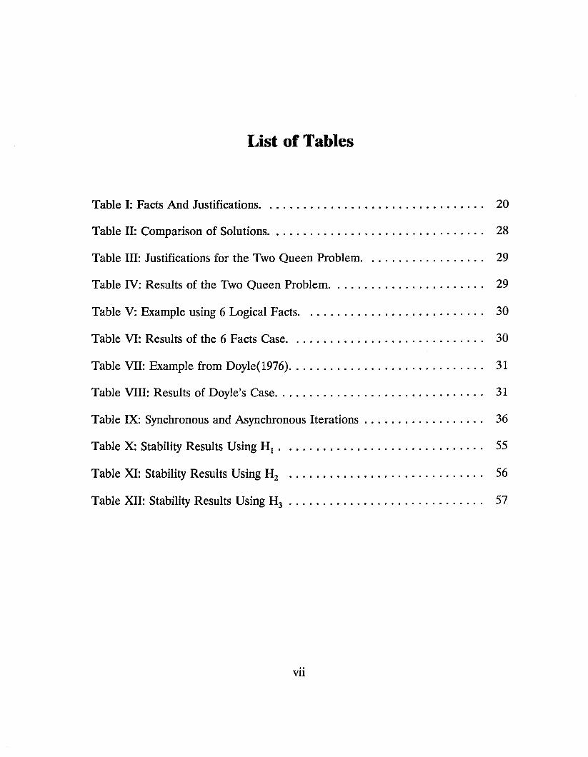
List of Tables

Table I: Facts And Justifications.............................................................................. 20

Table II: Comparison of Solutions........................................................................... 28

Table III: Justifications for the Two Queen Problem........................................... 29

Table IV: Results of the Two Queen Problem...................................................... 29

Table V: Example using 6 Logical Facts................................................................. 30

Table VI: Results of the 6 Facts Case..................................................................... 30

Table VII: Example from Doyle(1976).................................................................... 31

Table VIII: Results of Doyle’s Case........................................................................ 31

Table IX: Synchronous and Asynchronous Ite ra tio n s .......................................... 36

Table X: Stability Results Using H j ....................................................................... 55

Table XI: Stability Results Using H2 ................................................................... 56

Table XII: Stability Results Using H3 ................................................................... 57

vii

List of Figures

Figure 1: Basic Neuron Interconnections................................................................. 2

Figure 2: Basic Neural Network Architecture...................................................... 19

Figure 3: Electronic Circuit for TMS Neural N etw ork ....................................... 24

Figure 4: Two Queen Problem.................................................................................. 29

Figure 5: Iteration Graph for Synchronous M o d e l.............................................. 36

Figure 6: Iteration Graph Using Asynchronous Model .................................... 37

Figure 7: Types of Stability...................................................................................... 45

Figure 8: Immediate Neighborhood Points of the Origin.................................... 50

viii

ABSTRACT

A novel approach using Neural Networks has been developed to generate

consistent labelling of facts in relation to a given set of rules. In the proposed

system, facts are represented by neurons and their interconnections form the

knowledge base. The Neural Network Truth Maintenance System(TMS) arrives at

a valid solution provided the solution exists. A valid solution is a consistent

labelling of facts. If a valid solution does not exist the network does not converge.

An experimental setup was built and tested using conventional integrated circuits.

The hardware design is suitable for VLSI implementation for large, real-time

problems. The TMS Neural Network blends the simplicity and speed of Neural

Network architecture with the power of artificial intelligence techniques. A

methodology has been developed to study the stability of logical networks in terms

of Lyapunov Stability criteria.

1 Introduction

The development of Neural Networks is an attempt to mimic the operation

of the human brain. While traditional computers have taken a prominent place in

today’s technology even the most powerful computers have not matched the human

brain in solving certain types of problems in real time. For example speech

recognition is carried out by the human brain much faster than traditional

computers. The primary reason for the difference in performance can be attributed

to the parallel processing that occurs in the operation of the human brain in

contrast to the sequential processing in a traditional computer.

A traditional computer essentially has a central processing unit (CPU), and

many memory locations that have specific memory addresses. The CPU fetches

instructions sequentially from the memory locations and performs the necessary

operations. During this time all the other data/instructions residing in the memory

locations are sitting idle with no contribution to the throughput of the system. The

sequential processing is therefore a big bottleneck in the processing speed of a

traditional computer.

The concept of parallel processing has been introduced where several CPU

units processed the data in parallel. But the parallel processing is limited to

1

independent processes, and the overall computation process is essentially sequential.

The only difference is that different parts of the entire sequence of operations that

are independent, are processed simultaneously. The context of parallel processing

in the human brain is completely different. Every memory cell that contains data,

collectively act to produce the output. Study of the biological structure of the

human brain has indicated that the concept of a CPU does not exist in the human

brain. The detailed operation of the human brain is not clear yet and has not been

completely understood. However, current research in Neural Networks is based on

the gross organization of the brain cells.

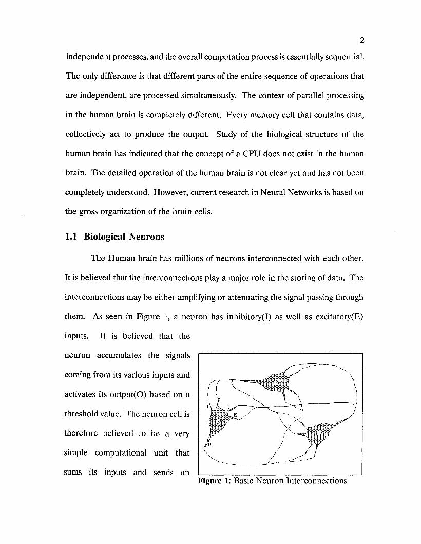
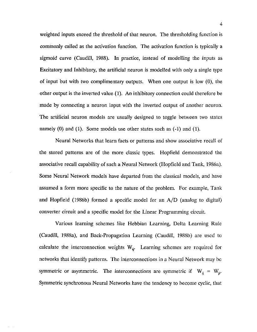
1.1 Biological Neurons

The Human brain has millions of neurons interconnected with each other.

It is believed that the interconnections play a major role in the storing of data. The

interconnections may be either amplifying or attenuating the signal passing through

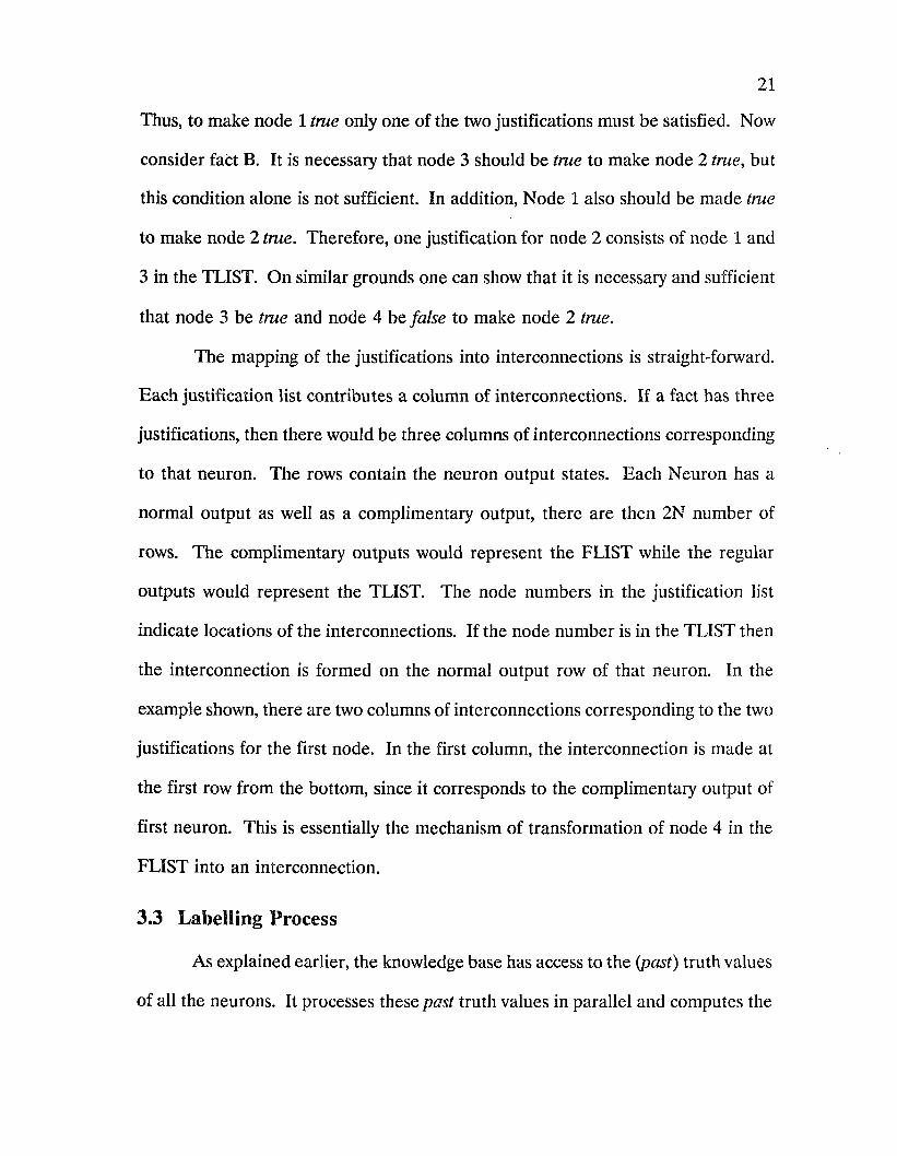
them. As seen in Figure 1, a neuron has inhibitory(I) as well as excitatory(E)

inputs. It is believed that the

neuron accumulates the signals

coming from its various inputs and

activates its output(O) based on a

threshold value. The neuron cell is

therefore believed to be a very

simple computational unit that

sums its inputs and sends anFigure 1: Basic Neuron Interconnections

output signal if the sum is above a threshold value. The attenuation or weight

factor associated with the interconnection may be a result of the length of the

interconnecting links. New links may be formed as new data is learned, or existing

links may be strengthened on repeated learning, or sometimes, the interconnections

may vanish because of loss of memory. The key factor is that if a few cells cease

functioning, the brain will still function and reconstruct the data with some minor

loss in detail (Hopfield, 1986). In fact the remaining cells may reconfigure during

another learning phase to compensate for the loss. A traditional CPU on the other

hand will halt if one memory location malfunctions.

1.2 Artificial Neurons

A Neural Network modelled after the brain is a set of computational units

whose interconnections are analogous to the interconnection between biological

neurons. In general, any model that resembles the interconnections of a biological

neuron has been classified as a Neural Network. Each computational unit has an

output and some inputs. Each input of the neuron is connected to an output of

another unit. In some cases one input of the neuron may be connected to its own

output, this is termed self or direct feedback (Caudill, 1987). The interconnections

are through amplifiers with gains ranging from 0 to > 1. The gains of these

amplifiers are generally called as weights.

A neuron is said to be triggered or ’fired’ when its output goes high (or a

logic level 1). The Excitatory inputs have a positive effect in triggering a neuron

in contrast to the Inhibitory inputs. A neuron is triggered when the sum of all the

weighted inputs exceed the threshold of that neuron. The thresholding function is

commonly called as the activation function. The activation function is typically a

sigmoid curve (Caudill, 1988). In practice, instead of modelling the inputs as

Excitatory and Inhibitory, the artificial neuron is modelled with only a single type

of input but with two complimentary outputs. When one output is low (0), the

other output is the inverted value (1). An inhibitory connection could therefore be

made by connecting a neuron input with the inverted output of another neuron.

The artificial neuron models are usually designed to toggle between two states

namely (0) and (1). Some models use other states such as (-1) and (1).

Neural Networks that learn facts or patterns and show associative recall of

the stored patterns are of the more classic types. Hopfield demonstrated the

associative recall capability of such a Neural Network (Hopfield and Tank, 1986a).

Some Neural Network models have departed from the classical models, and have

assumed a form more specific to the nature of the problem. For example, Tank

and Hopfield (1986b) formed a specific model for an A /D (analog to digital)

converter circuit and a specific model for the Linear Programming circuit.

Various learning schemes like Hebbian Learning, Delta Learning Rule

(Caudill, 1988a), and Back-Propagation Learning (Caudill, 1988b) are used to

calculate the interconnection weights W^. Learning schemes are required for

networks that identify patterns. The interconnections in a Neural Network may be

symmetric or asymmetric. The interconnections are symmetric if Wjj = Wjj.

Symmetric synchronous Neural Networks have the tendency to become cyclic, that

is, the network outputs a sequence of states and finally repeats a particular

sequence of states (Martland, 1987). If all neurons in a Neural Network update

their states simultaneously, the Neural Network is synchronous. If the updating is

randomly sequential that is, one neuron at a time is updated, the Neural Network

is asynchronous. Based on the nature of the intermediate states of a neuron,

Neural Networks are further classified into discrete or continuous networks.

Discrete Neural Networks (Vidal et al., 1987) have the same advantage over analog

Neural Networks as digital circuits have over analog circuits that is immunity to

noise in the small signal range.

The Neural Network model presented in this paper is of the discrete type,

where the only valid states of a neuron are a T or a ’O’. The Neural Network is

also an asymmetric asynchronous system. The Truth Maintenance System (TMS)

Neural Network model is different from the classic Hopfield model conceptually as

well as architecturally. The classic Hopfield model arrives at solutions (patterns)

that are stored in the Network in terms of the interconnection weights. The known

solutions are used to teach the Hopfield network to find the interconnection weights

via the learning schemes mentioned above. Once the interconnection weights are

determined, the network will converge to one of the stored patterns closest to the

given arbitrary input pattern. This type of memory access system is known as

associative memory. However, in the TMS Neural Network the interconnections are

fixed by the user based on rules and the solutions are not known apriori as is

explained in the following sections. Besides, the TMS Network is asymmetric,

compared to the symmetric network of Hopfield.

1.3 Expert Systems

One application of Neural Networks is in Expert Systems. The TMS Neural

Network (as would be shown later) could also be adapted as an Expert System. A

brief description of an Expert System is therefore included.

Expert Systems (Patrick and Winston, 1984) are essentially computer

programs that make use of knowledge and inference procedures to solve problems

that require human intelligence. The user provides facts and rules to the expert

system while the Expert System provides its expertise in solving the problem for the

user. The Expert System thus has a knowledge base and an inference engine. The

knowledge base consists of rules relating various facts present in the system.

Inferencing is arriving at a conclusion, which follows from given facts and the rules

present in the knowledge base. For example, assume that a knowledge base

contains the following rules regarding automobile diagnostics for a car that car does

not start:

(1) If ENGINE CRANKS and SPARK PLUGS FIREthen FUEL SYSTEM IS FAULTY

(2) If BATTERY IS LOWthen ALTERNATOR IS BAD or BATTERY IS BAD.

(3) If SPARK PLUGS DO NOT FIREthen BATTERY IS LOW or IGNITION COIL IS FAULTY

(4) If ENGINE DOES NOT CRANKthen BATTERY IS LOW

Note that the words in uppercase are facts and the if-then statements are the

rules that link the facts. The part before then is called the antecedent and the part

after then is called consequence. These rules are stored in a tree format so that it

is easy to search through the tree. Given a fact that the engine is not cranking, the

inferencing program searches through the rule tree using a search technique among

the antecedent part of the rule and finds a match with Rule #4. Rule #4 indicates

LOW BATTERY is a probable cause. The inferencing program then searches for

LOW BATTERY among the antecedents and finds a match with Rule #2. There

are two consequences for Rule # 2 namely BAD ALTERNATOR, BAD

BATTERY. The inferencing program then branches out and tries to find either of

the two consequence in the antecedent part of the rules but finds no match. The

inferencing program therefore arrives at two possibilities for the cause, namely a

bad alternator or a bad battery. In practice, the knowledge data base is large and

require complex search techniques.

The basic Truth Maintenance System is explained in Chapter 2. Chapter 3

is a literature search of related topics. The proposed TMS Neural Network is

explained in chapter 4. Chapter 5 details the hardware aspects of the system.

Example problems and simulation results are given in chapter 6. Modelling aspects

of the TMS Neural Network are covered in Chapter 7. Stability computations of

the TMS Neural Network are presented in Chapter 8. The final chapter concludes

the dissertation with suggestions for future work.

2 Truth Maintenance Systems

Consider a logic system system containing a finite number of facts. In the

current context, a fact is considered to be a description of an entity or process. The

facts are interrelated by rules. In the Truth Maintenance System a fact is restricted

to have two labels - true or false. The rules are lists of truth values that make a

particular fact true. Note that the words true and false are merely symbolic and may

be substituted by any set of labels that are complimentary to each other logically.

The labels true and false will be used from now on for the sake of convenience.

Each rule may use the truth values of some or all of the remaining facts. The truth

value for any fact is justified if at least one rule associated with that fact is satisfied.

If the truth values of all facts are justified, then the truth values are said to be

consistent.

A TMS algorithm solves for a consistent set of truth values for a set of facts

stored in a knowledge base. The state of the art TMS makes use of a recursive

labelling algorithm (Doyle, 1979) involving list manipulations. Such an algorithm

is well suited for implementations in LISP (List Processing). In practice the

number of facts that are stored in the TMS is very large. For a set of N facts, there

are 2N possible combinations of true/false values of which only a few combinations

8

may be consistent.

To understand the concept of facts and consistent truth values, consider a

system of facts as shown below:

FACT #1: (A) = CLOUDY SKY

FACT #2: (B) = RAIN

FACT #3: (A->B) = CLOUDY SKY implies RAIN

FACT #3: (NA) = Not CLOUDY SKY

In the above system there are 4 facts. If we assign truth values (a truth

value can be True (T) or False (F)) to each fact in the following order: T F T F

then by looking at the facts we can conclude by using our own logical reasoning that

the truth values namely T F T F are not consistent among each other with respect

to the rules defined above. This conclusion can be arrived at by the following

reasoning. It is trivial that the first (T) and fourth (F) truth values are consistent

with each other. The first truth value (T) tells us Sky is Cloudy. Since Fact #3 is

assigned True we can conclude that it will rain. However the second truth

value(F) indicates NO RAIN. Therefore we have an inconsistency or contradiction

in the set of truth values T F T F. Though this was a very simple example with

only four facts, we can see that the reasoning chain is complex. Since the actual

number of possible combinations of truth values are 2N for N number of facts, the

total number of combinations of the truth values in the above example is 16. For

a large problem with thousands of facts, the total number of combinations of truth

values become tremendously large. For such a large problem, one can imagine how

long it would take to find out even one set of consistent truth values.

10

2.1 Some More Terms and Definitions in a TMS

For a formal definition of a Truth Maintenance System consider a system

containing a finite number of facts. Let the truth value of each fact be dependent

on a number of rules. A fact can have one of two truth values - True or False.

Each rule may use the truth values of some or all of the remaining facts. The truth

value for any fact may be justified if at least one rule associated with that fact is

satisfied. If the truth values of all facts are justified, then the truth values are said

to be consistent. A Truth Maintenance System solves for a consistent set of truth

values for a set of facts stored in a knowledge base. The knowledge base contains

rules for determining truth values of the facts. The format of the rule storage is

discussed in more detail in the following chapters.

2.2 Applications and Importance

An expert system contains a rule database, and an inference engine. As

more and more rules are added, there is a distinct possibility of having conflicts

between the most recent rules and the existing rules in the database. This could

lead to faulty inferences. The TMS system would therefore be a valuable tool in

maintaining the consistency in the rule database. The TMS system can also be used

as an expert system. For example, to see if Fact 1 and Fact 2 imply Fact 3, Fact

3 (which is the goal node) is clamped to a false state, while the nodes for Fact 1

and Fact 2 are clamped true. If the system arrives at a consistent solution, then the

implication of the goal is False. The inference of the goal would be true only if the

11

system does not reach a consistent solution, i.e, it keeps oscillating. Thus to make

inferences, one has to only clamp the appropriate truth values. By clamping a truth

value for a particular node, the node is not allowed to be updated. It is said to be

locked.

The proposed TMS Neural Network model generates consistent truth values

for a given set of facts and rules. The TMS Neural Network is based on the

representation given by Doyle (1979). Doyle (1979) uses a generalized notion of

in and out instead of true and false representation. By in Doyle implies that the

corresponding fact is in the current set of beliefs otherwise, it is not in the set of

beliefs.

The TMS Neural Network model reduces the computation time by a large

factor when compared with a software implementation of the conventional labelling

algorithm on a traditional computer. The reduction in computation time can be

attributed to the massively parallel computation process that takes place in a Neural

Network. To our knowledge, there are no Neural Network models reported in the

literature, which uses the concept of TMS in arriving at consistent truth values.

Considering the simplicity in structure of the model combined with the speed of

obtaining solutions, the TMS Neural Network would be a significant step in

applying Neural Networks to expert system applications.

2.3 Conventional TMS Methodology

The significance of the TMS Neural Network will be perceived if one can

get an idea of the relative complication involved in obtaining the valid solutions

12

using conventional methods. A simplified version of Doyle’s algorithm (Kundu,

1989) is explained here for clarity. The algorithm begins with initializing all facts

to arbitrary truth values. A process of elimination begins by considering the truth

value (label = true/false) of the first fact and examining the justification lists of all

other facts. It may be recalled that each justification has two lists (a) TLIST and

(b) FLIST. For each justification a check is made to see if the label (true/false) of

fact #1 is same as the name of the list (TLIST/FLIST) to which it belongs. If the

check is positive, then the first fact number is eliminated from the appropriate list

in the justification in question. For instance, if fact #1 was labeled true and it was

found in the TLIST of a particular justification (say for fact #3), the first fact is

removed from the TLIST of the justification. If at this stage, the justification (say

for fact #3) becomes a pair of null sets, then the label of fact #3 is made true

irrespective of the previous assumption. Fact #1 is then called the justifier of the

justification being considered. If the check is negative then the entire justification

under scrutiny is removed. Again at this stage, if there are no justifications for a

particular fact remaining, then that fact is labeled false. This process is repeated

by considering fact # 2 and so on until the last fact. In the above process, it is

possible to arrive at a label for fact #1, contradictory to the one assumed. One

then has to back up to the point where the truth value of fact #1 was assumed, and

repeat the above process after changing the assumption for fact #1.

The above explanation is a brief outline of the concept of the labelling

process used in conventional AI techniques. In actual practice, the state of

13

computation is kept track of so that one knows how much to back up whenever a

contradiction takes place. The actual details of the process are not important to

this discussion since the purpose is to grasp the computational rigor involved in

arriving at a valid labelling.

2.4 Prior Work

An extensive search of published literature revealed no prior work on a TMS

Neural Network. However, work has been reported on implementing inferencing

in hardware. Inferencing involves arriving at conclusions based on a given set of

rules and initial facts. If the truth values are graded then the inference is a called

fuzzy inference. An inference engine is a processor that processes rules according

to a particular technique. Each updating process in a TMS Neural Network can be

considered as an inference step.

Kemke (1987) provides mathematical definitions of neurobiological terms.

He shows the similarities of the models of human neuron operations occurring in

neural networks. He shows that by selecting appropriate parameters the neurons

could behave as flip-flops and logical functions such as AND, OR and NOT. This

representation of neurons agrees very much with the TMS Neural Network model.

McNaughton and Papert (1971) also refer to neurons as a type of flip-flop.

Many hardware implementations of inferencing reported in the literature

make use of a hybrid architecture involving an external computer and are primarily

aimed at arriving at a conclusion. Some implementations store rules in ROM

(Read Only Memory). Cleary (1987) describes a VLSI chip in which the

communication between neurons is multiplexed. The VLSI chip is accessed by a

host computer and performs the mathematical operations or thresholding. One

application of the VLSI chip suggested is for rule based type of reasoning as used

in expert systems. In his system he assigns one unit (neuron) to each rule, fact, and

conclusion present in the expert system. A rule is said to fire if each of its

preconditions is true. This is programmed by setting the threshold equal to the

number of preconditions. This operation is similar to the logical AND function

with the number of inputs equal to the number of preconditions. A conclusion is

considered true if there is any rule that makes the conclusion and is firing. Simple

true / false reasoning is possible in this system and the author claims that the

system is very fast and could be part of an expert system where speed is important.

Some researchers have considered the modifications of search trees that are

extensively used in expert systems. One such work is based on Fuzzy Cognitive

Maps (FCMs) that are feedback generalizations of search trees. Kosko (1987)

considers an FCM as a form of Neural Network. He builds a connection matrix

having weights of 0, +1, and -1. The connection matrix is used for inferencing.

Each iteration of an inference consists of multiplying an input vector with the

weight matrix. The process is repeated by using the product of the previous

iteration until a limit cycle is reached. That is, the FCM stabilizes to a limit cycle.

He argues that convergence is obvious in at most 2N iterations since there are only

2n possibilities. He claims that in practice the convergence is obtained in very few

15

iterations. Comparisons of limit cycles (Taber and Siegel, 1987) of FCMs based on

different experts have also been studied.

Another approach taken by Green and Michalson (1987) uses a network

similar to an inference net. A node essentially has a summing junction for its

weighted inputs with a particular activation level. The node gives a boolean result

based on the inputs. They call their network an Evidence Flow Graph (EFG). The

graph essentially shows the links between the input hypothesis and Knowledge

Source Procedures (KSPs). The KSPs then evaluate all their inputs based on the

above method. The technique lacks specific mapping procedures to map decision

process into an EFG.

Another inference net approach was taken by Venkatasubramanian (1985)

who designed a parallel network expert system to deal with inexact or probablistic

reasoning. He used a parallel network of binary, threshold units. The solution was

obtained by a probabilistic search through the solution space using the simulated

annealing algorithm. The simulated annealing algorithm is a probablistic technique

in which the system is excited so that the current state is capable of escaping from

a local minima, and finally letting the system settle down at a new local minimum.

His architecture had three levels of nodes (1) input data nodes that were clamped

either in the on state or the o ff state depending on the observed symptoms of the

problem, (2) the intermediate level nodes that were driven by the nodes at the same

level along with the data supplied by the input nodes, and (3) the answer nodes that

represented the decision reached by the system. The number of levels for the class

16

of intermediate nodes depend on the problem. Knowledge was represented by the

weighted interconnections between the nodes. The weights were initially assigned

randomly, and were refined by comparing the outputs with the real world data.

There is no mention of any hardware implementation and an explicit rule

formulation is not given.

Optical implementation of expert systems (McAulay, 1987), (Warde and

Kottas, 1986), (Eichmann and Caulfield, 1985), (Szu and Caulfield, 1987) have also

been reported in the literature.

In all the literature reviewed (except McNaughton and Papert, 1971) none

of the implementations make use of the flip-flop model of a neuron. The TMS

Neural Network stands out uniquely, based on its capability to detect consistency

among all the facts in the database. At the same time, the TMS Neural Network

allows for inferences to be made as explained in the previous section.

Many references were found in the literature on the discrete analysis of

networks. Robert(1986) treated boolean networks as discrete iterations and used

the incidence matrix approach to study the convergence properties. This technique

is covered in more detail in Chapter 6. Thomas and Richelle (1988) obtains

relations for the number of steady states based on the number of positive loops in

the interaction graph. A graph with n positive loops may have up to 3" steady

states. He claims that interactions between the loops reduce the number of steady

states. A graph of interactions is a signed directed graph using the logical ’OR’

operator for the connection. The signed property of the connecting links represent

17

INVERTORS. This N element signed graph is then converted into a NxN adjacency

matrix which has the elements 0 ,1 , -1, depending on the connections. Thomas and

Richelle claim that this adjacency matrix is analogous to the Jacobian matrix of the

continuous systems. But, they conclude that their technique does not generalize

when the loops interact with each other. They described gene interactions in terms

of logical equations to use their technique. Apparently gene interaction seems to

be another area of application of TMS Neural Networks.

Bankovic (1989) shows that for a set of boolean equations that are

consistent, it is possible to arrive at a solution by the method of successive

elimination. This technique may be therefore used to verify the consistency of the

boolean equations. However, this technique would be more of a brute-force type

approach and involves symbolic computation.

3 TMS Neural Network Model

The TMS Neural Network embodies the following functions, (1) Fact

representation, (2) Knowledge representation, and (3) Labelling or Inferencing

process. A hardware implementation of the Network is also shown along with an

example problem. The conceptual architecture is shown in Figure 1. There is only

one layer of neurons that act as the input as well as the output neurons. This layer

is directly interconnected based on the rules involving the neurons.

3.1 Fact Representation

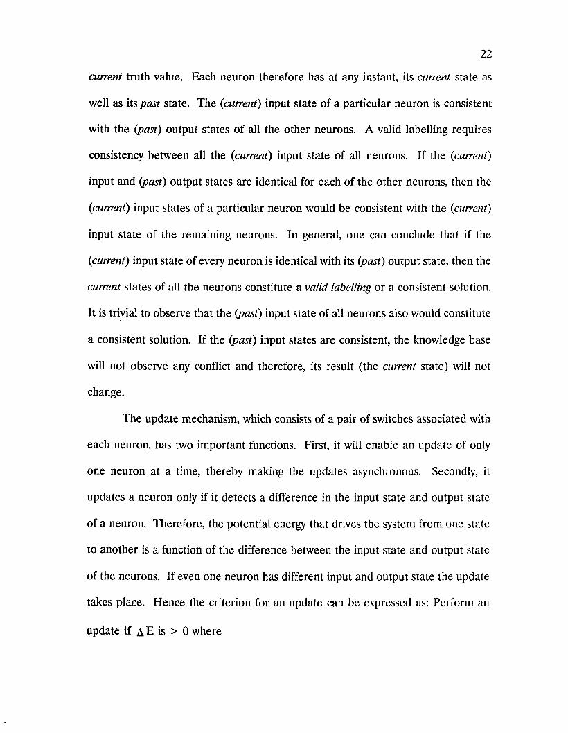
Each neuron represents a fact. The context of a fact is the same as

described in the earlier chapter. As seen from Figure 1, each neuron has an input

state as well as an output state. The input states of all neurons are volatile, i.e,

their states are determined by the instantaneous outputs of the knowledge base.

The output states on the other-hand store the input state values that were present

during triggering. The input or output state of a neuron can be either 0 or 1. For

simplicity in the hard-wiring, the inhibitory inputs are realized by having

complimentary (inverted) neuron outputs besides the regular neuron output. The

combined output states of these neurons form the output of the system. The inputs

19

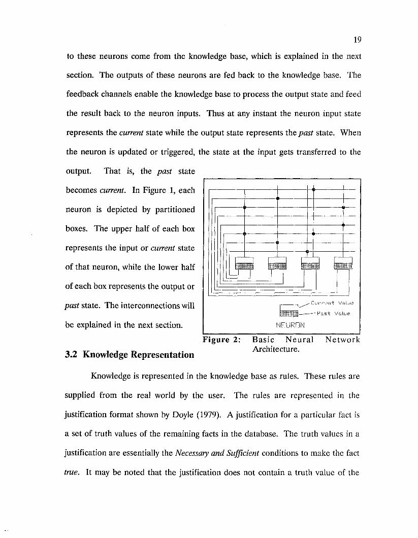
to these neurons come from the knowledge base, which is explained in the next

section. The outputs of these neurons are fed back to the knowledge base. The

feedback channels enable the knowledge base to process the output state and feed

the result back to the neuron inputs. Thus at any instant the neuron input state

represents the current state while the output state represents the past state. When

the neuron is updated or triggered, the state at the input gets transferred to the

output. That is, the past state

becomes current. In Figure 1, each

neuron is depicted by partitioned

boxes. The upper half of each box

represents the input or current state

of that neuron, while the lower half

of each box represents the output or

past state. The interconnections will

be explained in the next section.

3.2 Knowledge Representation

Knowledge is represented in the knowledge base as rules. These rules are

supplied from the real world by the user. The rules are represented in the

justification format shown by Doyle (1979). A justification for a particular fact is

a set of truth values of the remaining facts in the database. The truth values in a

justification are essentially the Necessary and Sufficient conditions to make the fact

true. It may be noted that the justification does not contain a truth value of the

C u r r e n t Va l ue

— P a s t V a l ue

im m

N E U R O N

rigu re 2: B asic N eu ra l N etw orkArchitecture.

2 0

same fact. In other words, there is no self-feedback present in the system.

As mentioned before a justification contains the truth values of several facts.

Facts are identified by node numbers. To identify the facts as well as their truth

values, each justification is separated into two lists, namely the TLIST and the

FLIST. The TLIST contains the node numbers of the facts that are true while the

FLIST contains the node numbers of the facts that are false.

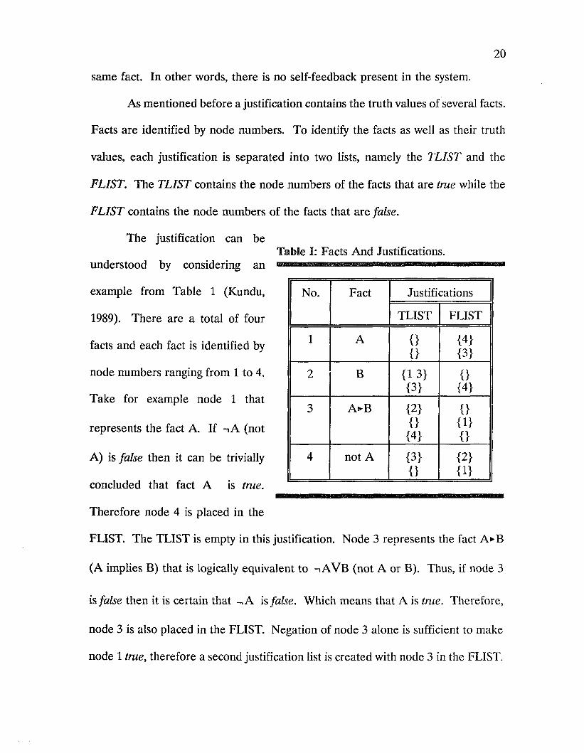
The justification can beTable I: Facts And Justifications.

understood by considering an

example from Table 1 (Kundu,

1989). There are a total of four

facts and each fact is identified by

node numbers ranging from 1 to 4.

Take for example node 1 that

represents the fact A. If -iA (not

A) is false then it can be trivially

concluded that fact A is true.

Therefore node 4 is placed in the

FLIST. The TLIST is empty in this justification. Node 3 represents the fact A^B

(A implies B) that is logically equivalent to -iAVB (not A or B). Thus, if node 3

is false then it is certain that -.A is false. Which means that A is true. Therefore,

node 3 is also placed in the FLIST. Negation of node 3 alone is sufficient to make

node 1 true, therefore a second justification list is created with node 3 in the FLIST.

No. Fact Justifications

TLIST FLIST

1 A {} {4}{} {3}

2 B {13} {}{3} {4}

3 A<*B {2} 0{} {1}

{4} {}

4 not A {3} {2}{} {1}

2 1

Thus, to make node 1 true only one of the two justifications must be satisfied. Now

consider fact B. It is necessary that node 3 should be true to make node 2 true, but

this condition alone is not sufficient. In addition, Node 1 also should be made true

to make node 2 true. Therefore, one justification for node 2 consists of node 1 and

3 in the TLIST. On similar grounds one can show that it is necessary and sufficient

that node 3 be true and node 4 be false to make node 2 true.

The mapping of the justifications into interconnections is straight-forward.

Each justification list contributes a column of interconnections. If a fact has three

justifications, then there would be three columns of interconnections corresponding

to that neuron. The rows contain the neuron output states. Each Neuron has a

normal output as well as a complimentary output, there are then 2N number of

rows. The complimentary outputs would represent the FLIST while the regular

outputs would represent the TLIST. The node numbers in the justification list

indicate locations of the interconnections. If the node number is in the TLIST then

the interconnection is formed on the normal output row of that neuron. In the

example shown, there are two columns of interconnections corresponding to the two

justifications for the first node. In the first column, the interconnection is made at

the first row from the bottom, since it corresponds to the complimentary output of

first neuron. This is essentially the mechanism of transformation of node 4 in the

FLIST into an interconnection.

3.3 Labelling Process

As explained earlier, the knowledge base has access to the {past) truth values

of all the neurons. It processes these past truth values in parallel and computes the

2 2

current truth value. Each neuron therefore has at any instant, its current state as

well as its past state. The (current) input state of a particular neuron is consistent

with the (past) output states of all the other neurons. A valid labelling requires

consistency between all the (current) input state of all neurons. If the (current)

input and (past) output states are identical for each of the other neurons, then the

(current) input states of a particular neuron would be consistent with the (current)

input state of the remaining neurons. In general, one can conclude that if the

(current) input state of every neuron is identical with its (past) output state, then the

current states of all the neurons constitute a valid labelling or a consistent solution.

It is trivial to observe that the (past) input state of all neurons also would constitute

a consistent solution. If the (past) input states are consistent, the knowledge base

will not observe any conflict and therefore, its result (the current state) will not

change.

The update mechanism, which consists of a pair of switches associated with

each neuron, has two important functions. First, it will enable an update of only

one neuron at a time, thereby making the updates asynchronous. Secondly, it

updates a neuron only if it detects a difference in the input state and output state

of a neuron. Therefore, the potential energy that drives the system from one state

to another is a function of the difference between the input state and output state

of the neurons. If even one neuron has different input and output state the update

takes place. Hence the criterion for an update can be expressed as: Perform an

update if a E is > 0 where

M 1, 0] (Eq.2)

and Fjj is the input state of the neuron j and Foj is the output state of neuron j.

When a consistent solution is obtained a E becomes zero. The system can then

be considered to have come to a minimum energy state. As long as there is conflict

among the past states, the system will keep searching for a consistent labelling.

Stability aspects of the network will be shown in later chapters.

3.4 Expert System Application

The TMS Neural Network could be used as an expert system by clamping

the truth values of the antecedent facts and the consequent facts. For example to

verify if Fact #1 implies Fact #3 of an imaginary TMS Neural Network, the truth

value of Fact #1 is clamped to a ’1’ and the truth value of Fact #3 is clamped to

a ’O’. If the network converges, then the implication Fact #1 implies Fact #3 is

false. If the network does not converge then the implication is true.

4 Hardware Implementation

An Integrated Circuit (IC) design of the Network using CMOS

(Com plim entary M etal Oxide

Semiconductor) chips is shown in

Figure 3. The Network has

interconnected AND gates, and OR

g a te s . E ach co lu m n of

interconnections corresponding to a

particular neuron represents an

AND gate. The AND gates ensure

that all nodes in a particular

justification satisfy the required

conditions. The outputs of all AND

gates of a particular neuron are connected to an OR gate. The OR gates allow

choice of any justification that becomes true. The output of each AND gate is

connected to one input of the OR gate. The output of each OR gate is connected

to the neuron input. Thus, the current state of each neuron is represented by the

output of an OR gate.

□ s c

Figure 3: Electronic Circuit for TMS Neural Network

24

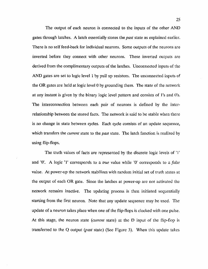
25

The output of each neuron is connected to the inputs of the other AND

gates through latches. A latch essentially stores the past state as explained earlier.

There is no self feed-back for individual neurons. Some outputs of the neurons are

inverted before they connect with other neurons. These inverted outputs are

derived from the complimentary outputs of the latches. Unconnected inputs of the

AND gates are set to logic level 1 by pull up resistors. The unconnected inputs of

the OR gates are held at logic level 0 by grounding them. The state of the network

at any instant is given by the binary logic level pattern and consists of l ’s and 0’s.

The interconnection between each pair of neurons is defined by the inter

relationship between the stored facts. The network is said to be stable when there

is no change in state between cycles. Each cycle consists of an update sequence,

which transfers the current state to the past state. The latch function is realized by

using flip-flops.

The truth values of facts are represented by the discrete logic levels of T

and ’O’. A logic ’1’ corresponds to a true value while ’0’ corresponds to a false

value. At power-up the network stabilizes with random initial set of truth states at

the output of each OR gate. Since the latches at power-up are not activated the

network remains inactive. The updating process is then initiated sequentially

starting from the first neuron. Note that any update sequence may be used. The

update of a neuron takes place when one of the flip-flops is clocked with one pulse.

At this stage, the neuron state (current state) at the D input of the flip-flop is

transferred to the Q output (past state) (See Figure 3). When this update takes

26

place, the new value will alter the current states of the remaining neurons,

depending on the interconnections. After the propagation delay, which is of the

order of nanoseconds (CMOS Data Book, 1981), all neuron inputs stabilize to the

appropriate new logic states.

Clock pulses are supplied by an oscillator at point A (Figure 3). The

updating procedure is minimal, in the sense that clock pulses for updating are not

sent to those neurons (flip-flops) that have identical current and past states. This

is achieved for each neuron by a pair of switches controlled by an XOR gate that

monitors the past and current state of that neuron. The switches associated with a

given neuron direct the clock pulses to the other neurons or to itself, depending on

the past and current states of the neuron in question. The switching arrangement

allows only one neuron to be updated at a time. If stability is reached then the

clock pulses start appearing at point B (Figure 3).

In order for the network to be used as an expert system, the truth values of

’0’ or T are clamped by using the RESET and SET inputs of the flip-flop.

Modification of the update mechanism is also necessary to prevent the update of

the clamped flip-flop.

5 Example Problems

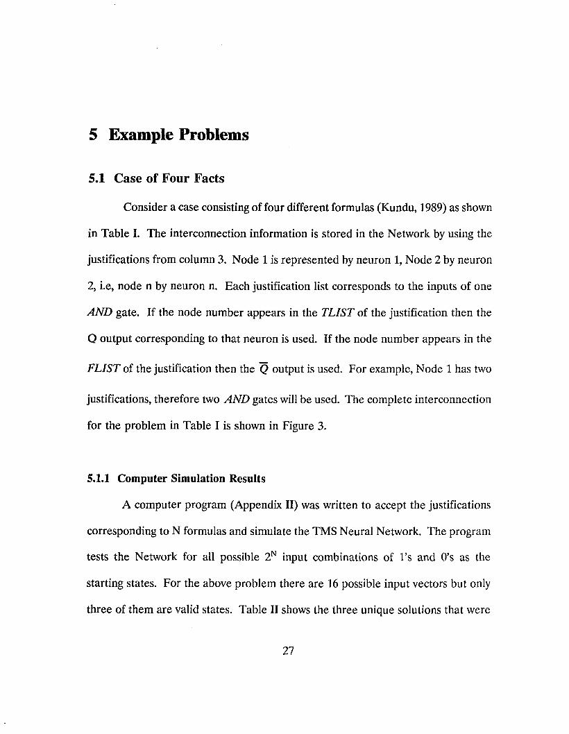
5.1 Case of Four Facts

Consider a case consisting of four different formulas (Kundu, 1989) as shown

in Table I. The interconnection information is stored in the Network by using the

justifications from column 3. Node 1 is represented by neuron 1, Node 2 by neuron

2, i.e, node n by neuron n. Each justification list corresponds to the inputs of one

AND gate. If the node number appears in the TLIST of the justification then the

Q output corresponding to that neuron is used. If the node number appears in the

FLIST of the justification then the Q output is used. For example, Node 1 has two

justifications, therefore two AND gates will be used. The complete interconnection

for the problem in Table I is shown in Figure 3.

5.1.1 Computer Simulation Results

A computer program (Appendix II) was written to accept the justifications

corresponding to N formulas and simulate the TMS Neural Network. The program

tests the Network for all possible 2N input combinations of l ’s and 0’s as the

starting states. For the above problem there are 16 possible input vectors but only

three of them are valid states. Table II shows the three unique solutions that were

27

28

obtained by this program compared to the conventional labelling algorithm. Note

that the conventional labelling algorithm would be implemented in LISP and would

require more computation time than the Neural Network to arrive at a valid

labelling.

5.1.2 Experimental Results

An experimental setup Table II: Comparison of Solutions,

was constructed of CMOS IC’s

with the interconnections

shown in Figure 3. LED’s were

used to indicate the output

states of individual neurons.

Table II shows that the

solutions were same as those obtained by the computer simulation. The clock

frequency was slowed to about 1 Hz, so that one could visually see the updates

taking place. With no clamping, each time the circuit was switched on, the network

began with a random set of truth values for the past states of each neuron, and

subsequently arrived at one of the stable states. The solution was observed almost

instantaneously when the clock was stepped up to 1 Mhz.

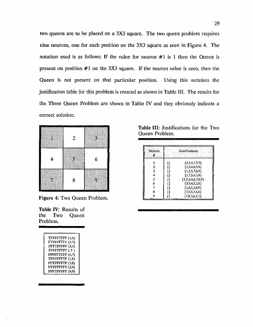
5.2 Eight Queen Problem

Another interesting example is the eight queen problem. The goal is to

place eight queens on an empty chess board such that no queen can attack another

queen. This problem is simplified and adapted to the TMS Neural Network so that

Conventional TMS Neural Network

Simulation

TMS Neural Network

Experimental

TTTF TTTF TTTFFFTT FFTT FFTT

TFFF TFFF TFFF

29

two queens are to be placed on a 3X3 square. The two queen problem requires

nine neurons, one for each position on the 3X3 square as seen in Figure 4. The

notation used is as follows: If the value for neuron #1 is 1 then the Queen is

present on position #1 on the 3X3 square. If the neuron value is zero, then the

Queen is not present on that particular position. Using this notation the

justification table for this problem is created as shown in Table III. The results for

the Three Queen Problem are shown in Table IV and they obviously indicate a

correct solution.

1 2 3

4 5 6

7 8 9

Figure 4: Two Queen Problem.

Table IV: Results of the Two Queen Problem.

TFFFFTFFF (1,6) FTFFFFTFF (2,7) FFTTFFFFF (3,4)

FFFFFTTFF (6,7) TFFFFFFTF (1,8)

FTFFFFFFT (2,9) FFFTFFFFT (4,9)

Table III: Justifications for the Two Queen Problem.

Neuron#

Justifications

1 {} {2,3,4,7,5,9}2 {} {1,3,4,6,5,8}3 {} {1,2,5,7,6,9}4 {) {1,7,5,6,2,8}5 {} {1,2,3,4,6,7,8,9}6 {} {3,9,4,5,2,8}7 {} {1,4,5,3,8,9}8 {} {7,9,5,2,4,6}9 {} {7,8,3,6,5,1}

30

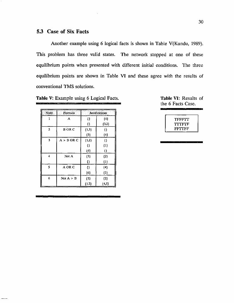
5.3 Case of Six Facts

Another example using 6 logical facts is shown in Table V(Kundu, 1989).

This problem has three valid states. The network stopped at one of these

equilibrium points when presented with different initial conditions. The three

equilibrium points are shown in Table VI and these agree with the results of

conventional TMS solutions.

Table V: Example using 6 Logical Facts. Table VI: Results ofw f l w w i i mmii'iiii—iiiiiHiiiiiiii the 6 Facts Case.

TFFFTT TTTFTF FFTTFF

Node Formula Justifications

1 A {} {4}

{} {3,2}

2 B O R C {1,3} {}{3} {4}

3 A > B OR C {1,2} {}

{} {1}{4} {}

4 Not A {3} {2}

{} {1}5 A O R C {} {4}

{6} {2}6 Not A > B {1} {2}

{1.2} {4,5}

31

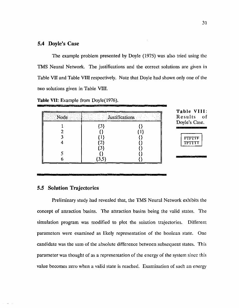
5.4 Doyle’s Case

The example problem presented by Doyle (1975) was also tried using the

TMS Neural Network. The justifications and the correct solutions are given in

Table VII and Table VIII respectively. Note that Doyle had shown only one of the

two solutions given in Table VIII.

Table VII: Example from Doyle(1976).

T a b l e V I I I :R e s u l t s of Doyle’s Case.

FTFTTFTFTTTT

5.5 Solution Trajectories

Preliminary study had revealed that, the TMS Neural Network exhibits the

concept of attraction basins. The attraction basins being the valid states. The

simulation program was modified to plot the solution trajectories. Different

parameters were examined as likely representation of the boolean state. One

candidate was the sum of the absolute difference between subsequent states. This

parameter was thought of as a representation of the energy of the system since this

value becomes zero when a valid state is reached. Examination of such an energy

Node Justifications

1 {3} {}2 {} {1}3 {1} {}4 {2} {}

{3} {}5 {} {}6 {3,5} {}

32

trajectory had shown unusual behavior of traversing over peaks and valleys before

coming to a minimum of zero. The plots of these trajectories are shown in

Appendix I as dark lines. Another parameter that was examined was the center o f

gravity in terms of the l ’s present in the boolean state. For example the center of

gravity for 0110 as well as for 1001 would be (1x1 + lx4 )/(l + 1) = 2.5. It was

hypothesized that the trajectory of the center of gravity would exhibit the

convergence toward the center of gravity of the valid state. The light colored line

of Appendix I indicates the center of gravity of the state trajectory. However study

of both the above trajectories did not reveal any interesting behavior.

6 TMS Neural Network as an Iterative Process

As mentioned before, the TMS Neural Network is a sequential updating

network. The system essentially produces an output state based on an input state.

The new output is fed back into the system to produce another output state. This

process is repeated until the output state becomes equal to the input state. The

operation of the TMS Neural Network can therefore be thought of as a discrete

iterative process. Francois Robert(1976) visualized the boolean iterative network

as an iteration graph and obtained several results. In this chapter, the results

developed by Robert(1976) will be applied to the TMS Neural Network. The

iteration graph of the TMS Neural Network for example 1 will be shown in the

subsequent sections of this chapter.

An iterative process can be mathematically described as given in(Eq.3):

X r n = F { X r) 0r = 0,1,2,...) (E9-3)

Where X and F are n dimensional vectors whose components are given by (Eq.4)

Since X is a n-dimensional vector, the above operation constitutes a synchronous

update mechanism. This is because, the output states of all neurons are computed

simultaneously based on the current input state. However, in the TMS Neural

33

X2 i=f2(Eq.4)

r+1 /. / r r r\Xn =fn{X l ’X2 > -Xn)

Network, only one neuron is allowed to compute the output and feed the result to

all other neurons. For modelling purposes, an operator is necessary that will map

the sequential update to a synchronous update. This will allow us to express the

asynchronous network operation in the format shown above. One candidate is the

Gauss-Seidel operator.

6.1 Gauss-Seidel Operator

The Gauss-Seidel operator will allow the updates, one neuron at a time,

though it may appear that all neurons are being updated simultaneously. The Gauss-

Seidel operator is applied as shown in (Eq.5):

= / i ( * p X2>-">Xn)

8 2{X V - S „ ) = / 2(£l(*)> X2’ - > Xn)

8 n(X V - ^ n ) = fn (8 !<*)» 82&>’ - 8 n - lV > ’ Xn)

(Eq.5)

Note that, the synchronous iteration for the TMS Neural Network is simpler to

express mathematically based on the interconnections. The Gauss-Seidel operator

35

can then be applied to incorporate the sequential update sequence. The update

sequence is determined by the order in which the equations are arranged. In the

above formulation the update sequence is 1, 2,..., i, ...n. The conversion is shown for

the following example.

6.2 Asynchronous Model of Example 1

From the relationships represented by the justifications in Table I, we obtain

the mathematical equations in terms of boolean logic as given by (Eq.6):

f x(x) = T3 + X4

f 2(x) = x xx3 +jCyX4 (Eq.6)f 3(x) = x2 + x x + x4

f 4(x) = x^x2 + x~x

Note that the OR operator is represented by +, the AND operator is represented by

multiplication, and the summation 1 + 1 is equal to 1 in boolean logic.

After applying the Gauss-Seidel operator and simplifying the boolean

expressions, we obtain (Eq.7) for an update sequence of 1,2,3,4:

g x(x) = 73 + x~4

g 2(x) = x ^ 4 (E q < 7)

g 3(x) = x3 + x4

g 4(x) = X4

6.2.1 Iteration Graphs

The iteration graph for the above problem can be obtained by considering all

possible vectors as an input and their corresponding output after one iteration. The

36

calculation is performed using synchronous as well as asynchronous operations

namely f(x) and g(x) respectively.

Table IX: Synchronous and Asynchronous Iterations

Figure 5 shows the iteration ■

graph for the synchronous update

model(Eq.6). The graph consists of

segments connecting the input state

code for x (column 1 of Table IX)

and output state code (column 4) as

calculated in Table IX. Note that

there are two graphs that are cyclic.

Starting from an initial state 2, 15,

or 6 the system cycles between states

6 and 15. Starting from an initial

state of 9, 12, 13, or 10, the systemm

cycles between 10 and 13. For all

other initial states except, 8 and 14 the

system reaches a fixed point namely, 3.

The other two fixed points 8 and 14 are

isolated fixed points. The fixed points

(3, 8, and 14) are defined as stable

states.Figure 5: Iteration Graph for SynchronousModel [F(x)]

INPUT SynchronousO/P

AsynchronousO/P

Code X F(x) Code G(x) Code

0 0 0 0 0 1 0 11 11 1 0 0 0 8

1 0 0 0 1 1 0 1 1 11 1 0 11 11

2 0 0 1 0 1 1 1 1 15 1 1 1 0 14

3 0 0 11 0 0 11 3 0 0 11 3

4 0 1 0 0 1 0 11 11 1 0 0 0 8

5 0 1 0 1 1 0 11 11 1 0 11 11

6 0 1 1 0 1 1 1 1 15 1 1 1 0 14

7 0 1 1 1 0 0 11 3 0 0 11 3

8 1 0 0 0 1 0 0 0 8 1 0 0 0 8

9 1 0 0 1 1 0 1 0 10 1 0 11 11

10 1 0 1 0 1 1 0 1 13 1 1 1 0 14

11 1 0 11 0 1 1 1 7 0 0 11 3

12 1 1 0 0 10 10 10 1 0 0 0 8

13 1 1 0 1 10 10 10 1 0 11 11

14 1 1 1 0 1 1 1 0 14 11 1 0 14

15 1 1 1 1 0 1 1 0 6 0 0 11 3

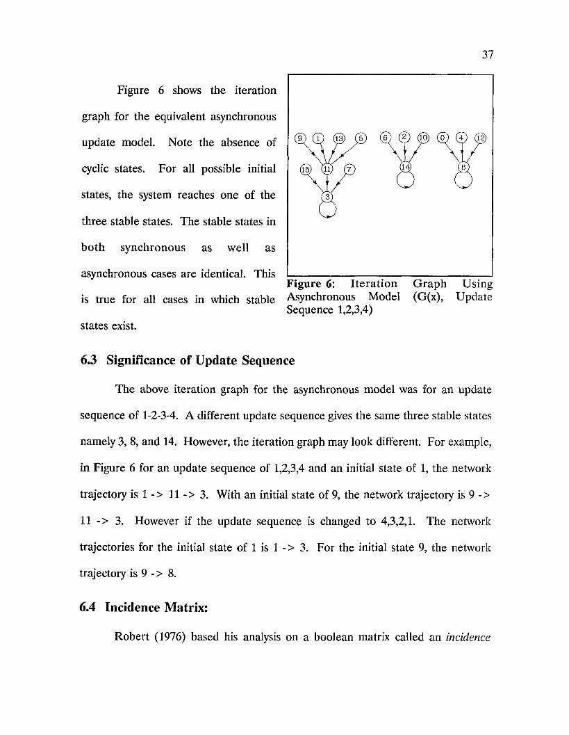
Figure 6 shows the iteration

graph for the equivalent asynchronous

update model. Note the absence of

cyclic states. For all possible initial

states, the system reaches one of the

three stable states. The stable states in

both synchronous as well as

asynchronous cases are identical. This

is true for all cases in which stable

states exist.

6.3 Significance of Update Sequence

The above iteration graph for the asynchronous model was for an update

sequence of 1-2-3-4. A different update sequence gives the same three stable states

namely 3, 8, and 14. However, the iteration graph may look different. For example,

in Figure 6 for an update sequence of 1,2,3,4 and an initial state of 1, the network

trajectory is 1 -> 11 -> 3. With an initial state of 9, the network trajectory is 9 - >

11 -> 3. However if the update sequence is changed to 4,3,2,1. The network

trajectories for the initial state of 1 is 1 -> 3. For the initial state 9, the network

trajectory is 9 - > 8.

6.4 Incidence Matrix:

Robert (1976) based his analysis on a boolean matrix called an incidence

37

5

14]

Figure 6: Itera tion G raph UsingAsynchronous Model (G(x), Update Sequence 1,2,3,4)

38

matrix. The incidence matrix of F is defined to be a NxN boolean matrix given by

(Eq.8):B(F) = b{.

where b.j = 0 i f f t is independent o f Xj and btj = 1 i f f . is dependent o f xj

The incidence matrix for the synchronous system (Eq.6) is given by (Eq.9)

(Eq.8)

B(F)

0 0 1 1 1 0 1 1 1 1 0 0 1 1 1 0

(Eq.9)

For the asynchronous system (Eq.7) the incidence matrix is given by(Eq.lO):

B(G) =

0 0 1 1 0 0 1 1 0 0 1 1 0 0 0 1

(Eq.10)

The incidence matrix however seems to be a crude tool to study the stability

because it carries very little information about the relationship between the state

variables. It is also possible to have the same incidence matrix for a stable as well

as an unstable system. A counter example that discourages the use of incidence

matrix is shown next.

39

Consider the system (E q .ll), which does not have any equilibrium points,

gi(x) = x3 + x4 g2(x) = x^ 4 g jx ) = x3 + x4 g4(x) = x4

(E q.ll)

The incidence matrix is given by (Eq.12)

B(G) =

0 0 1 10 0 1 1

0 0 1 1

0 0 0 1

(Eq.12)

Compared to the stable system (Eq.7) and its associated incidence matrix

(Eq.10), It could be seen that both (Eq.10) and (Eq.12) are same! Following this

discovery, the incidence matrix technique was abandoned.

7 Mathematical Modelling of TMS Neural Network

To study the stability of the TMS Neural Network it is necessary to generate

a mathematical model of the system. The mathematical model of the TMS Neural

Network can be described if we can model the individual components of the system.

The components of the system are logic gates and flip-flops. The motivation behind

developing the mathematical model is to find out the stability characteristics of the

system. An algebraic model would enable us to apply stability principles developed

by Lyapunov. It is therefore necessary for the system model to be completely

algebraic.

There are two basic approaches: (1) model the individual components used

in the hardware circuit and develop equations based on the hardware connections

between individual components; or (2) develop the equations for each neuron in

terms of the boolean functions implied by the justification table, and then convert

the boolean equations into the necessary algebraic form. Both techniques involve

development of simple algebraic relations for boolean operations. The use of the

first technique directly yields equations that incorporate the asynchronous update

operation. The second technique still would require some type of transformation to

incorporate the asynchronous update operation. Implementation of the first

technique involves substantial computation, also the computation would be different

40

41

for each problem. The first method was therefore abandoned.

The second technique involved development of the boolean equations to

model the operation of the individual neurons. This step was simple since the

justification table provided the logical relationships required for each neuron. The

sequential update information was then incorporated by using the Gauss-Seidel

operator(Sec. 6.1). The resulting boolean equations now closely represented the

asynchronous operation of the TMS Neural Network. The next step is to convert

these boolean equations into simple algebraic equations without the use of MAX or

ABS functions. The conversion of the boolean equations would require equivalent

algebraic operations corresponding to boolean operations namely AND, NOT, OR,

etc.

The algebraic model of each boolean operation can be devised by observing

the truth table of each logic element. The truth table of all the logic elements used

in the TMS Neural Network is shown below with the respective algebraic description.

All the models assume that the input states and output states take the logic states of

0 and 1.

7.1 AND Gate

The AND gate is the simplest to model algebraically and is described by the

product of the inputs. This model is also valid for multiple inputs. The algebraic

equation for an AND gate with three inputs A, B, and C and output as Q is given

by (Eq.13)

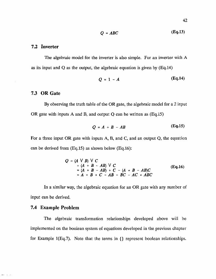
42

Q = ABC (Eq.13)

7.2 Inverter

The algebraic model for the inverter is also simple. For an inverter with A

as its input and Q as the output, the algebraic equation is given by (Eq.14)

Q = 1 - A (Eq.14)

73 OR Gate

By observing the truth table of the OR gate, the algebraic model for a 2 input

OR gate with inputs A and B, and output Q can be written as (Eq.15)

Q = A + B - AB (Eq.15)

For a three input OR gate with inputs A, B, and C, and an output Q, the equation

can be derived from (Eq.15) as shown below (Eq.16):

Q = {A V B) V C= (A + B - AB) V C (Eq.16)= (A + B - AB) + C - (A + B - AB)C = A + B + C - A B - B C - A C + ABC

In a similar way, the algebraic equation for an OR gate with any number of

input can be derived.

7.4 Example Problem

The algebraic transformation relationships developed above will be

implemented on the boolean system of equations developed in the previous chapter

for Example l(Eq.7). Note that the terms in {} represent boolean relationships.

43

The algebraic transformation is obtained as (Eq.17):

8 i ( x ) = {*3 + * 4}= (1 - JC3) + (1 - x4) - (1 - x3) (1 - x4)

= 1_ - *3 * 4

g 2(x) = {*3x4}= x3(l - *4) (Eq.17)

g 3(x) = {*3 + x4)= x3 + x4 - x3 x4

8&) = {*4}= *4

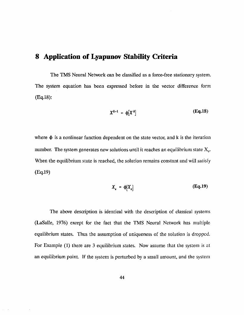
8 Application of Lyapunov Stability Criteria

The TMS Neural Network can be classified as a force-free stationary system.

The system equation has been expressed before in the vector difference form

(Eq.18):

Xk+l = <J>[X*] (Eq.18)

where <J> is a nonlinear function dependent on the state vector, and k is the iteration

number. The system generates new solutions until it reaches an equilibrium state Xe.

When the equilibrium state is reached, the solution remains constant and will satisfy

(Eq.19)

Xe = <j)[XJ (Eq.19)

The above description is identical with the description of classical systems

(LaSalle, 1976) except for the fact that the TMS Neural Network has multiple

equilibrium states. Thus the assumption of uniqueness of the solution is dropped.

For Example (1) there are 3 equilibrium states. Now assume that the system is at

an equilibrium point. If the system is perturbed by a small amount, and the system

44

45

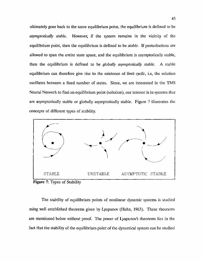
ultimately goes back to the same equilibrium point, the equilibrium is defined to be

asymptotically stable. However, if the system remains in the vicinity of the

equilibrium point, then the equilibrium is defined to be stable. If perturbations are

allowed to span the entire state space, and the equilibrium is asymptotically stable,

then the equilibrium is defined to be globally asymptotically stable. A stable

equilibrium can therefore give rise to the existence of limit cyclic, i.e, the solution

oscillates between a fixed number of states. Since, we are interested in the TMS

Neural Network to find an equilibrium point (solution), our interest is in systems that

are asymptotically stable or globally asymptotically stable. Figure 7 illustrates the

concepts of different types of stability.

STABLE UNSTABLE ASYMPTOTIC STABLE

Figure 7: Types of Stability

The stability of equilibrium points of nonlinear dynamic systems is studied

using well established theorems given by Lyapunov (Hahn, 1963). These theorems

are mentioned below without proof. The power of Lyapunov’s theorems lies in the

fact that the stability of the equilibrium point of the dynamical system can be studied

46

without the knowledge of the system trajectories or solution. This method can

therefore be applied to the stability analysis of the TMS Neural Network.

8.1 Terms and Definitions

Lyapunov’s direct method involves finding a scalar function called Lyapunov

Function with certain properties. These properties are explained below:

8.1.1 Positive Definite Function

A scalar function V(x) is positive definite if and only if both conditions (1) and

(2) hold

(1) V(x) is zero at the origin.-

(2) V(x) > 0 at all points in the state space other than the origin.

Note that a positive definite function is not allowed to be equal to zero at any

point other than zero.

8.1.2 Positive Semi-Definite Function

A scalar function V(x) is positive semi-definite if and only if condition (1)

holds

(1) V(x) > = 0 at all points in the state space other than the origin.

8.1.3 Negative Definite Function

A scalar function V(x) is negative definite if -V(x) is positive definite.

8.1.4 Negative Semi-Definite Function

A scalar function V(x) is negative semi-definite if -V(x) is positive semi

definite.

47

8.1.5 Positive Definite Matrix

A matrix H, can be positive definite if the following equivalent conditions are

true

1. The quadratic form of H, which is XTHX is positive definite

2. All the principal minors of H are greater than zero.

The principal minors of a matrix H, are calculated by computing the

determinants of the sub-matrices, with each diagonal element of H, as the first

element of the sub-matrix. For a NxN matrix there would be N principal minors.

The computation of the principal minors is carried out in the next chapter.

8.2 Lyapunov’s Stability Theorems

The stability of the equilibrium points of dynamical systems is classified into

three major categories namely (1) Stable Equilibrium, (2) Asymptotically Stable

Equilibrium, and (3) Unstable Equilibrium. According to Lyapunov, the three types

of stability can be defined based on a function. This function called the Lyapunov

function is based on the problem description, which is in terms of the derivative of

the state variables. Definitions of the different types of stability in terms of

Lyapunov functions are given below.

8.2.1 Stable Equilibrium

The equilibrium state X = 0 is stable if there exists a scalar function V(x) that

is positive definite and AV(X) is negative semi-definite. V(x) is called a Lyapunov

function.

48

8.2.2 Asymptotically Stable Equilibrium

The equilibrium state X = 0 is asymptotically stable if there exists a scalar

function V(X) that is positive definite and A F ( X ) i s negative definite.

Note that the stability definitions are defined with respect to the equilibrium

point at the origin. In the TMS Neural Network, the equilibrium points are usually

non-zero. This demands mapping the system equations so as to translate the

equilibrium to the origin.

8.3 Translation of the Equilibrium Point

The TMS Neural Network may have multiple equilibrium points none of

which may be at the origin of the system. However, all Lyapunov’s stability tests are

defined with respect to the origin as an equilibrium point. It therefore becomes

necessary to translate the equilibrium point to the origin and then test its stability.

The translation of the equilibrium point is carried out by the following procedure.

Using (Eq.18), (Eq.19) and with y as the transformed coordinate, we obtain

(Eq.20-a)-(Eq.20-c).

Y k = X k - X,e (Eq.20-a)

X k = Y k + Xe(Eq.20-b)

X*+1 = Yk+1 + Xe(Eq.20-c)

Substituting the above relations into the system equation (Eq.18) we get (Eq.21)

49

i'**1 - ♦(r* + X.) - X,Yk+1 - $(Yk) (Eq.21)

where®(Yk) = <t>(F* + Xe) - Xe

The translated system equation now has an equilibrium at Ye = [0 0 0 0] and will be

used later in the Lyapunov’s stability theorems.

8.4 Lyapunov Functions

Though Lyapunov provided a powerful technique to test the stability of the

equilibrium of a system, there is no general methodology to derive suitable Lyapunov

functions. The Lyapunov function may be different for different systems and are not

unique for a given system. Extensive work (Edward 1968, Vannelli 1985, Szego 1963)

has been done in the generation of Lyapunov functions but they are usually restricted

to specific class of problems. To prove the stability of an equilibrium point, one has

to search for a suitable Lyapunov function. Failure to find such a function still does

not guarantee instability. The technique however, guarantees stability, if a Lyapunov

function is found.

A common form of a Lyapunov functions is of the form (Eq.22)

y = [ yi y2 - y„ ]T (Eq.2 2 )V1(Y) = \ Y \

V! is obviously positive definite on st”

Another form used widely is (Eq.23)

In the limiting case, with H = I, we obtain V2 = YT1Y = YTY = V1

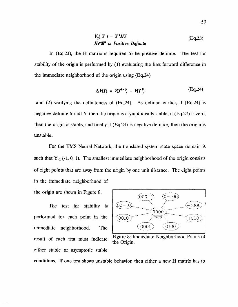
50

V2( Y ) = Y tHY (Eq.23)H e 81" is Positive Definite

In (Eq.23), the H matrix is required to be positive definite. The test for

stability of the origin is performed by (1) evaluating the first forward difference in

the immediate neighborhood of the origin using (Eq.24)

AF(Y) = V{Yk+1) - F(F*) (Eq.24)

and (2) verifying the definiteness of (Eq.24). As defined earlier, if (Eq.24) is

negative definite for all Y, then the origin is asymptotically stable, if (Eq.24) is zero,

then the origin is stable, and finally if (Eq.24) is negative definite, then the origin is

unstable.

For the TMS Neural Network, the translated system state space domain is

such that Y e{-l, 0, 1). The smallest immediate neighborhood of the origin consists

of eight points that are away from the origin by one unit distance. The eight points

in the immediate neighborhood of

the origin are shown in Figure 8. ___ ___(000-JJ (0-100)

The test for stability is X jooo)

performed for each point in the ( O O I O X ^ y o iic iiT s . XlQQo)

immediate neighborhood. The (^oooT) (o io o )

result of each test must indicate Immediate Neighborhood Points ofthe Origin.

either stable or asymptotic stable

conditions. If one test shows unstable behavior, then either a new H matrix has to

51

be tried or a new V(Y) has to be found. If an H matrix can be found such that all

tests indicate stable behavior then it can be concluded that the origin vis-a-vis the

equilibrium point in question is stable. The stability test has to be carried out for all

the equilibrium points in the system in a similar way.

9 Stability of TMS Neural Network

The concepts of stability developed in the previous chapter will be applied to

the TMS Neural Network example 1. The network function for each neuron is first

represented in boolean notation. This step is simple since the circuit is also a logic

circuit. The resulting boolean equations are shown below (Eq.25)

Equations (Eq.25) in fact represent the operation of the network in a synchronous

update mode. Since the TMS Network operates in asynchronous mode, the system

equations are transformed using the Gauss-Siedel operator (Sec. 6.1) as shown in

(Eq.26-a), (Eq.26-b) along with the intermediate boolean simplification steps. The

system (Eq.26-a), (Eq.26-b) shown is for an update sequence 1-2-3-4.

fx(x) = x3 + x4f 2(x) = x{x3 + x3x4f 3(x) = x2 + x^ + x4f 4(x) = xjx2 +

(Eq.25)

gfo) = * 3 + * 4

g2ix) = Xfa + *3*4

= ( f3 + * > 3 + *3*4 (Eq.26-a)

= 0 + x3x4 + x3x4= X3X4

52

£>(*> = X2 + *1 + X4= X3X4 + x 3 + x 4 + x 4= x jc 4 + XyX4 + X4= x 3(x4 + x4) + *4

= x3( 1 ) + *4= * 3 + X4

g 4(x) = x 3x2 + x x

= (x3 + x4) ( x ^ ) + X3~ T T 4

= (X3 + X4)(X3 + Xi) + X3X4= (x3x 3 + x3x4 + x / 3 + x4x4) + x # 4= (0 + x 3x4 + x4x 3 + x4) + X3X4= x 4(x3 + x 3 + 1 + x 3j

= x4a + 1)

The boolean equations (Eq.26-a)-(Eq.26-b) are then transformed into simple

algebraic equations using the relations developed earlier. The algebraic

simplification steps are shown below (Eq.27):

g x(x) = (1 - x3) + (1 - x4) - (1 - x3)(l - x4)= 1 x3x4

82(x) = h i 1 ~ x4) (Eq.27)= x 3 - x3x4

g 3{x) = x3 + x4 - x3x4

g4{x) = x4

Rewriting the algebraic equations in difference form we obtain (Eq.28).

53

(Eq.26-b)

£+1 . k kXi = 1 - X3x4

*2 - x3i1 x4 ) (Eq.28)‘(i - */)* + i *x3 = X3 + x4

*+1 kX4 = X4

54

As mentioned before, the TMS Neural Network often has multiple

equilibrium points. Since we are translating the system with respect to one

equilibrium point at a time. The origin represents only one of the equilibrium

points. The origin therefore cannot be a global attractor due to the presence of

other attractors in the state space. The stability analysis of the network with multiple

equilibrium points therefore has to restrict to the nearest neighborhood of the origin.

Using equations (Eq.28), one has to find an H matrix such that the first

forward difference (Eq.24) is greater then or equal to zero for all the immediate

neighborhood points of the equilibrium point. The H matrix is a 4x4 matrix, so to

make the search easier an interactive computer program was written (Appendix III).

The computer program makes use of the above equations along with the translation

equations (Eq.21) and computes the first forward difference (Eq.24) for each

neighborhood point of the equilibrium point, and evaluates their stability. Note that

after each translation, each equilibrium point becomes the origin of the system. The

neighborhood points in the translated state space would therefore be same for all the

three equilibrium points. The program displays the H matrix on the screen and

allows the user to edit the H matrix. The evaluation of the stability of all the three

equilibrium states for all their immediate neighborhood points is displayed on the

screen simultaneously. The user can keep changing the H matrix arbitrarily until the

desired results are obtained. Here, the H matrix was changed until at least one

equilibrium point had all its neighborhood points satisfy the Lyapunov criterion.

After several trials, it was possible to obtain an H matrix that made all the

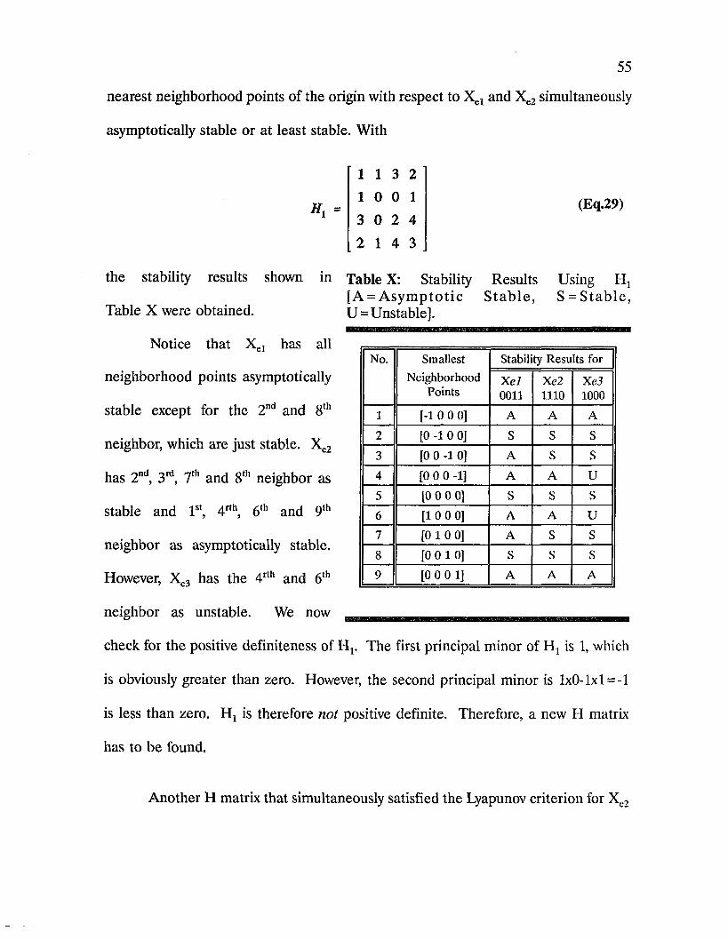
55

nearest neighborhood points of the origin with respect to Xel and Xe2 simultaneously

asymptotically stable or at least stable. With

1 1 3 2 1 0 0 1 3 0 2 4

2 1 4 3

(Eq.29)

the stability results shown in Table X: Stability Results Using Hj[A = A sy m p to tic S ta b le , S = S tab le ,

Table X were obtained. U=Unstable].

Notice that Xel has all

neighborhood points asymptotically

stable except for the 2nd and 8th

neighbor, which are just stable. Xe2

has 2nd, 3rd, 7th and 8th neighbor as

stable and 1st, 4rth, 6th and 9th

neighbor as asymptotically stable.

However, Xe3 has the 4rth and 6th

neighbor as unstable. We now

No. SmallestNeighborhood

Points

Stability Results for

X el0011

Xe21110

Xe31000

1 [-1 0 0 0] A A A

2 [0 -1 0 0] S S S

3 [0 0 -1 0] A S S

4 [0 0 0 -1] A A u5 [0 0 0 0] S S s6 [10 0 0] A A u7 [0 1 0 0] A S s8 [0 0 10] S S s9 [0 0 0 1] A A A

check for the positive definiteness of Hj. The first principal minor of is 1, which

is obviously greater than zero. However, the second principal minor is lxO-lxl = -l

is less than zero. H 3 is therefore not positive definite. Therefore, a new H matrix

has to be found.

Another H matrix that simultaneously satisfied the Lyapunov criterion for Xc2

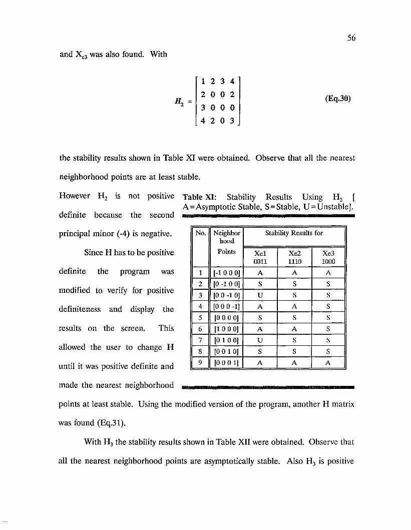
56

and Xe3 was also found. With

1 2 3 4

to 0 0 23 0 0 04 2 0 3

(Eq.30)

the stability results shown in Table XI were obtained. Observe that all the nearest

neighborhood points are at least stable.

However H2 is not positive Table XI: Stability Results Using H2 [A=Asymptotic Stable, S=Stable, U=Unstable].

definite because the second

principal minor (-4) is negative.

Since H has to be positive

definite the program was

modified to verify for positive

definiteness and display the

results on the screen. This

allowed the user to change H

until it was positive definite and

made the nearest neighborhood

points at least stable. Using the modified version of the program, another H matrix

was found (Eq.31).

With H3 the stability results shown in Table XII were obtained. Observe that

all the nearest neighborhood points are asymptotically stable. Also H3 is positive

No. Neighborhood

Points


X el0011

Xe21110

Xe31000

1 [-1 0 0 0] A A A

2 [0 -1 0 0] S S S

3 [0 0 -1 0] U S S

4 [0 0 0 -1] A A S

5 [0 0 0 0] S S s6 [1 0 0 0] A A s7 [0 1 0 0] U S s8 [0 0 10] s S s9 [0 0 0 1] A A A

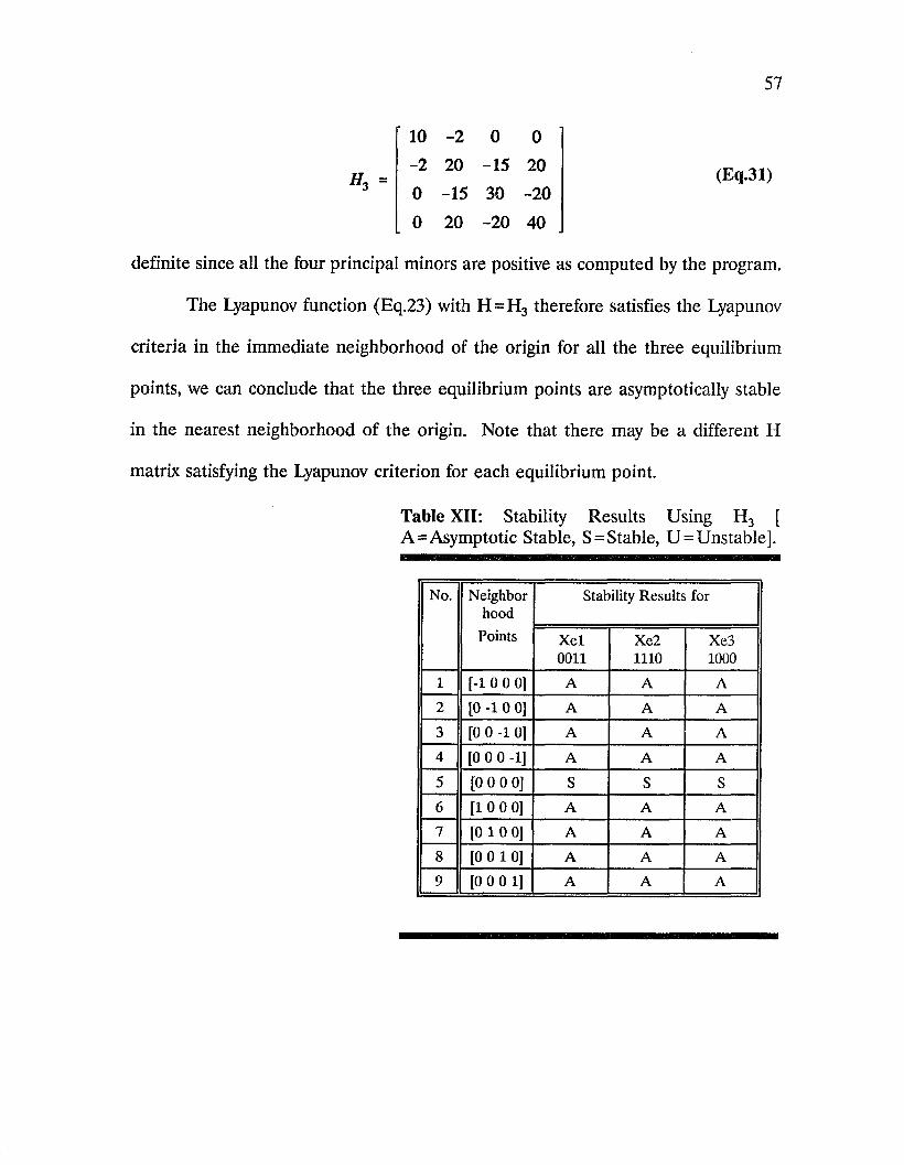
57

10 -2 0 0-2 20 -15 200 -15 30 -200 20 -20 40

(Eq.31)

definite since all the four principal minors are positive as computed by the program.

The Lyapunov function (Eq.23) with H = H 3 therefore satisfies the Lyapunov

criteria in the immediate neighborhood of the origin for all the three equilibrium

points, we can conclude that the three equilibrium points are asymptotically stable

in the nearest neighborhood of the origin. Note that there may be a different H

matrix satisfying the Lyapunov criterion for each equilibrium point.

Table XII: Stability Results Using H3 [A=Asymptotic Stable, S = Stable, U = Unstable].

No. Neighborhood

Points


X el0011

Xe21110

Xe31000

1 [-1 0 0 0] A A A2 [0 -1 0 0] A A A

3 [0 0 -1 0] A A A4 [0 0 0 -1] A A A

5 [0 0 0 0] S S S6 [10 0 0] A A A7 [0 1 0 0] A A A8 [0 0 10] A A A9 [0 0 0 1] A A A

10 Conclusions

10.1 Salient Features

In spite of the development of powerful techniques and representation models,

Artificial Intelligence (AI) has had a limited success in the application arena because

of lack of real time performance efficiency. Neural Networks on the other hand have

the unique capability of high speed by virtue of their parallel architecture. The TMS

Neural Network inherits the good features of both AI and Neural Networks with

respect to model representation and execution speed. The TMS Neural Network

model stands out uniquely from conventional Neural Network models functionally

as well as architecturally. Conventional Neural Networks are primarily aimed at

associative memory storage by generating the interconnection weights for a given set

of memories. For a TMS Neural Network the interconnection weights are known

apriori. Given an input the conventional Neural Network is expected to yield one

of the stored memories. However, the TMS Neural Network gives a solution that

is not known apriori. Of course, there are optimization applications of Neural

Networks that yield an unknown solution. Based on this context, the TMS Neural

Network would fit into the optimization application branch of Neural Networks.

The knowledge representation model of the TMS Neural Network makes it

58

59

unique when compared with other expert system implementations using Neural

Networks. The knowledge representation model allows the TMS Neural Network

to check for consistency in the knowledge (rule) base as more rules are added to it.

The TMS Neural Network system is as sensitive as a conventional TMS algorithm

to the addition or removal of rules or certain facts. This is in spite of the fact that

the algorithms are different from each other. This behavior was observed in the

initial stages of development of the TMS Neural Network and was very encouraging.

This partly contributed to the validity of the TMS Neural Network in the absence of

a convergence proof at the developmental stage.

The hardware is simple due to the absence of resistors and operational

amplifiers usually found in conventional Neural Networks. The TMS Neural

Network is based on logic and the interconnections are switches. This makes it more

reliable and less prone to noise problems. However it is possible to develop an

equivalent model using resistors and comparators. The neuron update operation of

the TMS Neural Network is also very simple and is driven by the difference between

the input state and output states. Our intuition agrees with this type of update since

the system is trying to reach a state of zero difference between the input and output

state. Overall, the concept of TMS has never been merged or implemented with

Neural Networks before.

The time required to arrive at a stable state is insignificant, considering the

high clock frequency that could be used. For very large problems a stable solution

would be found using a much higher clock frequency, say for example 10 MHz. The

60

high speed of inferencing lends this new system toward a real time expert system.

A true mathematical model of the TMS Neural Network that included the

asynchronous update process was constructed. A new methodology for applying the

modified Lyapunov stability criterion to the TMS Neural Network has also been

successfully devised. Application of the Lyapunov stability criterion has revealed that

the equilibrium points of the TMS Neural Network were asymptotically stable in the

nearest neighborhood of the origin. However since the system has multiple

equilibrium points, it would not be possible to find a Lyapunov Function for

satisfying Global Asymptotic Stability criterion. That is, the origin with respect to

one of the equilibrium points cannot be an attractor for the whole state space due

to the presence of other attractors.

10.2 Future Work

As mentioned before, the behavior of the system is different for different

update sequences. This behavior needs to be studied in greater detail. Knowledge

of the trajectory behavior in relation to the update sequence could be used for faster

convergence toward the solution. Also, the update sequence in the practical

implementation changes dynamically. Modelling of the dynamic update sequence

could therefore be undertaken in the near future.

The hardware implementation shown here demonstrated the operation of the

network. The practical implementation however involves many intricate details such

as interfacing of the network with traditional computers. The ultimate goal is to

fabricate the TMS Neural Network on a chip. Practical limitations of the number

61

of pins on a chip requires the use of multiplexing for loading and unloading of the

interconnection data. The circuit details necessary for loading the interconnection

data also need to be worked out.

References

Bankovic Dragic, 1989, Some Remarks on the Number of Parameters of The Solutions of Boolean Equations, Discrete Mathematics, 79(1989/90), pp229- 234.

Caudill, M., 1987, "Neural Networks PRIMER Part I", A I EXPERT, December, pp46-51.

Caudill, M , 1988a, "Neural Networks PRIMER Part II", A I EXPERT, February, pp55-61.

Caudill, M., 1988b, "Neural Networks PRIMER Part III", A I EXPERT, June, pp53-59.

Chang Chieh Hang, Chang, J.A., 1970, IEEE Transactions on Automatic Control, August 1970, pp 510-512.

Cleary, J. G.,1987, 'A simple VLSI connectionist architecture", IEEE First International Conference in Neural Networks, Vol iii, pp 419-426.

CMOS databook, 1981, National Semiconductor Corporation.

Dale F. Stewart and Edward T. Wall, 1969, A Matrix Transformation for the Direct Generation of Liapunov State Functions, ACTA TECHNICA CSAV, Prague, Czechoslovakia, No. 6., pp 667-682.

Doyle, J., 1979, 'A Truth Maintenance System", Artificial Intelligence, Vol 12, pp231-272.

Edward T. Wall, 1968, A Topological Approach To The Generation Of The Liapunov Functions, ACTA TECHNICA CSAV, Prague, Czechoslovakia, No. 2., pp 159-177.

Eichmann, G., and Caulfield, J. H., 1985, "Optical learning (inference) machines", Applied optics, Vol 24, No. 14, pp 2051- 2054.

Green, P. E, and Michalson, W. R., 1987, "Real Time Evidential Reasoning and Network based processing", IEEE First International Conference on Neural Networks, Vol ii, pp359-365.

62

63

Hahn W., 1963, Theory and Application of Lyapunov’s Direct Method, Prentice-Hall, Englewood Cliffs, NJ.

Hopfield, J. J., and Tank, D. W., 1986a, "Computing with Neural Circuits: A Model", Science, Vol 233, pp625-632.

Ingwerson D.R., 1961, A modified Lyapunov Method for Nonlinear Stability Analysis, IRE Transactions on Automatic Control, 1961, ppl99-210.

James A. Yorke, 1970, A Theorem on Lyapunov Functions Using V, Mathematical Systems Theory, Vol 4, No. 1., Springer-Verlag New York Inc., pp 40-45.

Kemke, C.,1987, "Modelling Neural Networks by means of Networks of Finite Automata", IEEE First International Conference on Neural Networks, Vol iii, pp23-29.

Kosko, B.,1987, 'Adaptive Inference in Fuzzy Knowledge Networks", IEEE First International Conference on Neural Networks, Vol ii, pp261-268.

Kundu, S., 1989, Advanced Artificial Intelligence Lecture Notes, Louisiana State University.

LaSalle J.P., 1976, The Stability of Dynamical Systems, Society for Industrial and Applied Mathematics, Philadelphia.

Lindorff D.P., 1965, Theory of Sampled Data Systems, John Wiley & Sons Inc., New York.

Maitra, K. K., 1961, "Stability of Logical Networks and Its application to Improvement of Reliability", IRE Transactions on Circuit Theory, September, pp335-341.

Martland, D., 1987, "Behavior of Autonomous (Synchronous), Boolean Networks, IEEE First International Conference on Neural Networks, Vol ii, pp243-250.

McAulay, A. D., 1987, "Real Time Optical Expert System", Applied Optics, Vol 26, No. 10, pp 1927-1933.

McNaughton, R., Papert, S., 1971, Counter-Free Automata , MIT Press.

Michel A.N., Sarabudha N.R., and Miller R.K., 1981, Stability Analysis of Complex Dynamical Systems, Circuits Systems Signal Process, Vol 1, No. 2, ppl71-202.

64

Robert F., 1986, Discrete Iterations - A Metric Study, Springer-Verlag Berlin.

Szego G.P., 1963, New Methods for Constructing Liapunov Functions for Time- invariant Control Systems, Proceedings o f the 2nd IFAC World Congress, Basel, 1963/1964.

Szu, H. H., and Caulfield, J. H., 1987, "Optical expert Systems", Applied Optics, Vol 26, No. 10.

Taber, W. R., and Siegel, M. A.,1987, "Estimation of expert weights using fuzzy cognitive maps", IEEE First International Conference on Neural Networks, Vol ii, pp319-325.

Tank, D. W., and Hopfield, J. J., 1986b, "Simple ’Neural’ Optimization Networks: An A /D Converter, Signal Decision Circuit, and a Linear Programming Circuit", IEEE Transactions on circuits and systems, Vol CAS-33, No.5, pp 533-541.

Thomas R., Richelle J., 1988, Positive Feedback Loops and Multistationarity, Discrete Applied Mathematics 19(1988), pp381-396.

Vannelli A., Vidyasagar M., 1985, Maximal Lyapunov Functions and Domains of Attraction for Autonomous Nonlinear Systems., Automatica, Vol 21, No. 1, pp69-80.

VenkataSubramanian, V., 1985, "Inexact Reasoning in Expert Systems: A Stochastic Parallel Network Approach", IEEE Computer Society Conference on A I Applications.

Vidal, J. J., Pemberton, J. C., and Goodwin, M.,1987, "Implementing Neural Nets with Programmable Logic", IEEE First International Conference on Neural Networks,Vol iii, pp 539-545.

Warde, C., and Kottas, J., 1986, "Hybrid optical inference machines: architectural considerations", Applied optics, Vol 25, No.6, pp 940-947.}

APPENDIX I

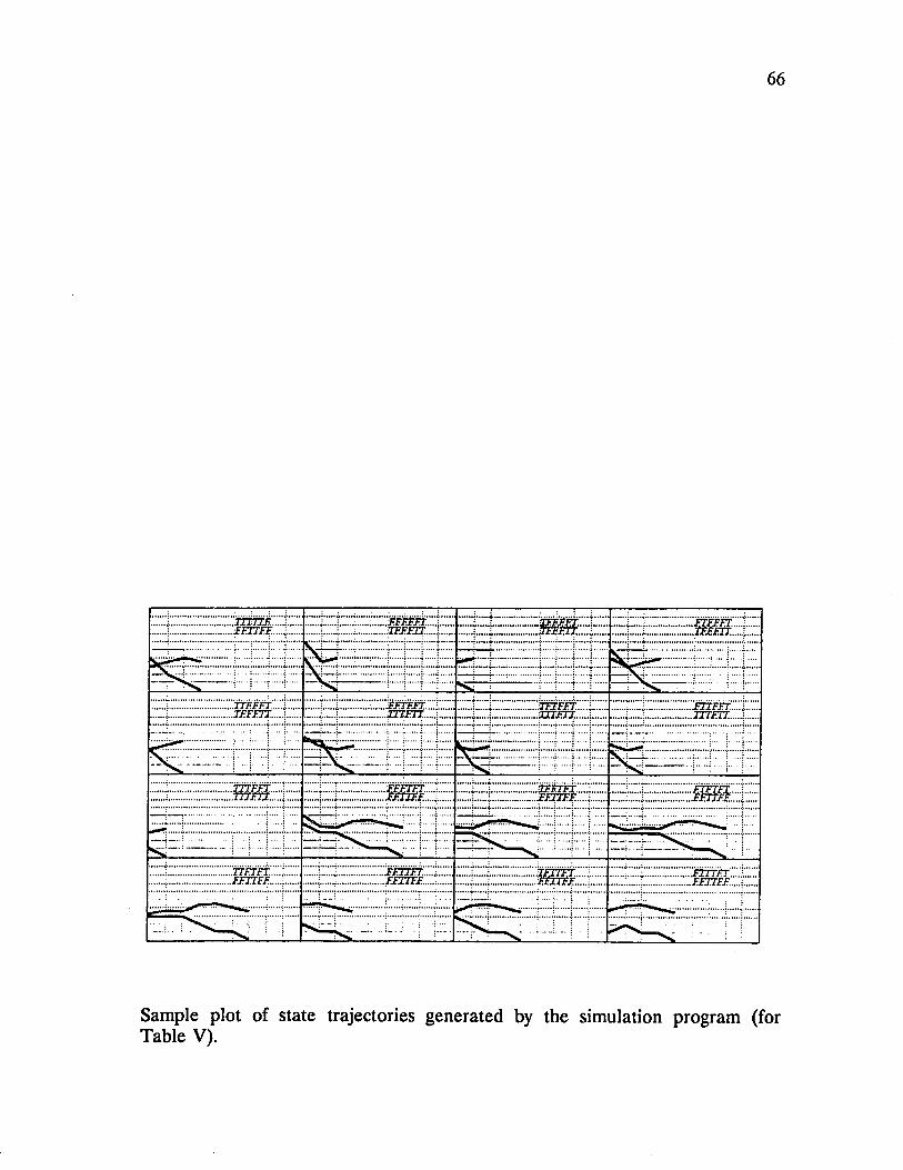
66

Sample plot of state trajectories generated by the simulation program (for Table V).

APPENDIX II

Source Code of Program SIMTMSNN.BAS

67

TMS Neural Network SIMULATOR

Program Written by: Suresh Guddanti Postscript Plotting support included

DEFINT I-NDECLARE SUB helpscreen ()DECLARE SUB postbox ()DECLARE SUB postlinel (xpsll, ypsll, xps21, yps2!, pthickl, pgray!) DECLARE SUB postpage ()DECLARE SUB postclose ()DECLARE SUB posttext (xpll, ypl!, ptex$)DECLARE SUB POSTLINE (xpll, ypl!, xp2!, yp2!, pthickl, pgray!) DECLARE SUB newstate ()DECLARE SUB stable ()DECLARE SUB allneuron ()DECLARE SUB negation ()DECLARE SUB plotreset ()DECLARE SUB convstate (s$)DECLARE SUB initplot ()DECLARE SUB plot ()DECLARE SUB initplotl (jb)DECLARE SUB tmsfast ()DECLARE SUB fastrulesl (i)DECLARE SUB regen ()DECLARE SUB wsort ()DECLARE SUB fastrules ()DECLARE SUB checkwt (i, j, k, iww)DECLARE SUB intersect (i)DECLARE SUB wvupdate (i)DECLARE SUB music ()DECLARE SUB default ()DECLARE SUB actvert (i, j)DECLARE SUB neuronl (i)DECLARE SUB settle ()DECLARE SUB automode ()DECLARE SUB dec2bcd (ib)DECLARE SUB consistent (i, v)DECLARE SUB sCIRCLEl (p, q, c)DECLARE SUB redraw ()DECLARE SUB delay (tm)DECLARE SUB getdata ()DECLARE SUB savedata ()DECLARE SUB vupdate (i)DECLARE SUB tms ()DECLARE SUB rules ()DECLARE SUB wupdatc (iww)DECLARE SUB wtredraw ()DECLARE SUB scircle (p, q, c)DECLARE SUB weights ()DECLARE SUB kcyinput ()DECLARE SUB neuron (i)DECLARE SUB vertical (i)DECLARE SUB horizontal (i)DIM SHARED xn(10,10, 20), yn(10,10, 20), aimage(lOOO), itr, id, abort DIM SHARED k$, ipast(lO), icurient(lO), xmax, x, invert(lO), noninvert(lO), DIM SHARED nwt, wx(100), wy(100), nvert(lO), wtcol, restart, rcstartl, dl DIM SHARED nlock(lO), order(lO), up$, ncycle, iw(100), kw(100), jw(100) DIM SHARED ksound, fl$, pulse(lOOO), npulsc, postprn DIM SHARED nwn(10,10), kkw(10, 10, 50)

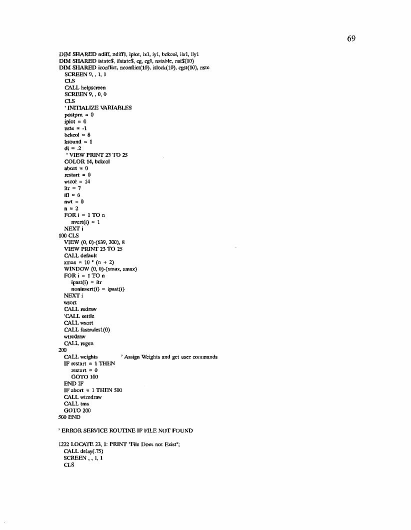
DIM SHARED ndiff, ndiffl, iplot, ixl, iyl, bckcol, ilxl, ilyl DIM SHARED istateS, ifstateS, eg, egl, nstable, nst$(10)DIM SHARED iconflict, nconflict(lO), islock(10), cgst(10), nste

SCREEN 9, , 1, 1 CLSCALL helpscreen SCREEN 9, , 0, 0 CLS’ INITIALIZE VARIABLESpostpm = 0iplot = 0nste = -1bckcol = 8ksound = 1dl = .2’ VIEW PRINT 23 TO 25

COLOR 14, bckcol abort = 0 restart = 0 wtcol = 14 itr = 7 ifl = 6 nwt = 0 n = 2FOR i = 1 TO n

nvert(i) = 1 NEXT i

100 CLS VIEW (0, 0)-(639, 300), 8 VIEW PRINT 23 TO 25 CALL default xmax = 10 * (n + 2)WINDOW (0, 0)-(xmax, xmax)FOR i = 1 TO n

ipast(i) = itr noninvert(i) = ipast(i)

NEXT i wsortCALL redraw ’CALL settle CALL wsort CALL fastrulesl(O) wtredraw CALL regen

200CALL weights ’ Assign Weights and get user commandsIF restart = 1 THEN

restart = 0 GOTO 100

END IFIF abort = 1 THEN 500 CALL wtredraw CALL tms GOTO 200

500 END

’ ERROR SERVICE ROUTINE IF FILE NOT FOUND

1222 LOCATE 23, 1: PRINT "File Does not Exist";CALL delay(.75)SCREEN , , 1,1 CLS

PRINT "Files in your directory;"PRINT "Files in your directory;"FOR i = 1 TO 30: PRINT : NEXT i FILESPRINT : PRINT : PRINTLOCATE 23, 1: INPUT "Load File; ", fl$CALL helpscreen SCREEN , , 0, 0FOR i = 1 TO 10: PRINT : NEXT i CLSRESUME

SUB actvert (i, j) xl = i * 10 + 10 + 5 / (nvert(i) + 1) * j LINE (xl, 18.5)-(xl, xmax), 11

END SUB

SUB allneuron FOR i = 1 TO n

CALL neuron(i)NEXT i END SUB

SUB automode CALL wsortIF iplot = 0 THEN nstable = 0IF iplot = 1 THEN CALL initplotpulset = 0pulsemax = 0FOR jb = 0 T O 2 ' n - lCALL dec2bcd(jb)IF iplot = 1 THEN CALL convstate(jstate$) istateS - jstateSIF iplot = 1 THEN CALL initplotl(jb)’ LOCATE 24, 1: PRINT b;

k$ = INKEYS IF k$ = "X" THEN

restart = 1IF iplot = 1 THEN CALL plotreset GOTO 899

END IFCALL tmsfastIF npulse > pulsemax THEN pulsemax = npulsc pulset = pulset + npulse pulse(B + 1) = npulse NEXT jbpulsea = pulset / 2 A n IF iplot = 0 THEN

LOCATE 23, 50: PRINT "Update Average = pulsea; LOCATE 24, 50: PRINT "Max. Updates = "; pulsemax; LOCATE 23, 1: PRINT SPACE$(48);LOCATE 23, 1: PRINT "Stable States :";FOR kkl = 1 TO nstable

PRINT nst$(kkl); " ";NEXT kkl

ELSECALL keyinput CALL plotreset

END IF 899

IF postprn = 1 THEN CALL postclose END SUB

71

SUB checkwt (i, j, k, iww) iww = 0FOR mw = 1 TO nwt

IF iw(mw) = i AND jw(mw) = j AND kw(mw) = k THEN iww = mw NEXT mw

END SUB

SUB consistent (i, v) v = 1: ndiff = 0: eg = 0 FOR ii = 1 TO n

IF ii = i THEN 543 IF ipast(ii) < > icurrent(ii) THEN

v = 0ndiff = ndiff + 1

END IF 543 NEXT ii

n2 = 0FOR ii = 1 TO n

IF ipast(ii) = itr THEN eg = eg + ii n2 = n2 + 1

END IF NEXTiiIF n2 = 0 THEN

eg = 0 ELSE

eg = eg / n2 END IF

END SUB

SUB convstate (s$) s$ = ""FOR i = 1 TO n

IFipast(i) = itr THEN s$ = s$ + "T"

ELSEs$ = s$ + "F"

END IF NEXT i END SUB

SUB dec2bcd (ia)FOR i = 1 TO n

ib = 2 A (i - 1) itemp = (ib AND ia) / ib ipast(i) = itrIF itemp = 0 THEN ipast(i) = ifl

NEXT iFOR i = 1 TO n

IF nlock(i) < > 0 THEN ipast(i) = islock(i)

END IF NEXT i’ IF iconflict = 1 THEN CALL negation

END SUB

SUB default up$ =FOR pi = 1 TO n

oider(pl) = piup$ = up$ + CHR$(48 + pi)

NEXT pi

72

LOCATE 24,1: PRINT "Update Sequence: up$;ixl = 1: iyl = 1 ilxl = 9: ilyl = 2

END SUB

SUB delay (tm) tl = TIMERWHILE ABS(TIMER - t l) < tm WEND

END SUB

SUB fastrulesl (ineuron)’ IF iconflict = 1 THEN CALL negation FOR i = 1 TO n

IF i = ineuron THEN 435 icurient(i) = ill FOR j = 1 TO nvert(i)

FOR nw = 1 TO nwn(i, j) temp = kkw(i, j, nw) / 2 itemp = INT(temp)IF (1 AND kkw(i, j, nw)) = 1 THEN

IF ipast(itemp + 1) = itr THEN GOTO 124

ELSE END IF

ELSEIF ipast(itemp) = ill THEN GOTO 124 ELSE END IF

END IF NEXT nw icurrent(i) = itr EXIT FOR

124 NEXT j 435 NEXT i

’ IF iconflict = 1 THEN CALL negation END SUB

SUB getdata ON ERROR GOTO 1222 LOCATE 24, 1: PRINT SPACE$(20);LOCATE 24, 1: INPUT "Load File: ", flS IF fl$ = "" THEN GOTO 134 OPEN fl$ FOR INPUT AS #1

INPUT #1, n, nwt FOR i = 1 TO nwt

INPUT #1, iw(i), jw(i), kw(i)NEXT iFOR i = 1 TO n

INPUT #1, nvert(i)NEXT iFOR i = 1 TO n

INPUT #1, nconflict(i)NEXT i CLOSE

134 LOCATE 24, 1: PRINT SPACE$(20);ON ERROR GOTO 0

END SUB

SUB helpscreenFOR i = 1 TO 25: PRINT : NEXT i

73

COLOR 14LOCATE 1, 30: PRINT "HELP SCREEN"COLOR 13LOCATE 3,10: PRINT "EDITING COMMANDS"LOCATE 4, 5: COLOR 14: PRINT "n/N"; : COLOR 3: PRINT ": Add/Delete Neuron"LOCATE 5, 5: COLOR 14: PRINT "a/A"; : COLOR 3: PRINT ": Add/Delete Justifications"LOCATE 6, 5: COLOR 14: PRINT "i/I"; : COLOR 3: PRINT ": Add/Delete Interconnection"COLOR 13LOCATE 8, 10: PRINT "FILE COMMANDS"LOCATE , 5: COLOR 14: PRINT T ’; : COLOR 3: PRINT ": Save problem to file"LOCATE , 5: COLOR 14: PRINT "r"; : COLOR 3: PRINT ": Retrive problem from file"LOCATE , 5: COLOR 14: PRINT "Z"; : COLOR 3: PRINT ": Specify PostScript filename"COLOR 13LOCATE 13, 10: PRINT "PLOTTING COMMANDS"LOCATE , 5: COLOR 14: PRINT "p"; : COLOR 3: PRINT ": Enable Plotting"LOCATE , 5: COLOR 14: PRINT "P"; : COLOR 3: PRINT ": Disable Plotting"COLOR 13LOCATE 3, 50: PRINT "SIMULATION COMMANDS"LOCATE , 45: COLOR 14: PRINT "t : COLOR 3: PRINT " : Toggle Neuron State"LOCATE , 45: COLOR 14: PRINT "y : COLOR 3: PRINT " : Enable Fast Settling"LOCATE , 45: COLOR 14: PRINT "e/E"; : COLOR 3: PRINT " : Enable/Disable Negation"LOCATE , 45: COLOR 14: PRINT "1 : COLOR 3: PRINT " : Lock neuron State"LOCATE , 45: COLOR 14: PRINT "o/O"; : COLOR 3: PRINT " : Change/Default Update Seq"LOCATE , 45: COLOR 14: PRINT "R : COLOR 3: PRINT ” : Reset all neuron states"LOCATE , 45: COLOR 14: PRINT "B : COLOR 3: PRINT " : Set to next binary state"LOCATE , 45: COLOR 14: PRINT "b : COLOR 3: PRINT " : Try all inputs"LOCATE , 45: COLOR 14: PRINT "X "; : COLOR 3: PRINT " : QUIT PROGRAM"LOCATE 22, 5: COLOR 14: PRINT "NOTE: KEYBOARD MUST BE IN NUMLOCK MODE FOR ARROWS TO WORK" END SUB

SUB horizontal (i)IF i = 0 THEN EXIT SUB noninvert(i) = ipast(i) invert(i) = itrIF noninvert(i) = itr THEN invert(i) = iflx = i * 10 + 10xl = x + 1.25x2 = x + 3.75yl = 13.5 -1 3 / n * iy2 = 13.5 - 13 / n * (i - 1)y = (yl + y2) / 2LINE (xl, 13.5)-(xl, y), invert(i)x3 = 20 -1 9 / n * (i)x4 = 20 - 19 / n * (i - 1)x4 = (x4 + x3) / 2LINE (x2, yl)-(x3, yl), noninvert(i)LINE (xl, y)-(x4, y), invert(i)xy = xmax - 23y3 = 18.5 + xy / n * iy4 = 18.5 + xy / n * (i - 1)y4 = (y3 + y4) / 2 + 1.5LINE (x3, yl)-(x3, y3), noninvert(i)LINE (x4, y)-(x4, y4), invert(i)LINE (x3, y3)-(xmax, y3), noninvert(i)LINE (x4, y4)-(xmax, y4), invert(i)LINE (x2, 13.5)-(x2, yl), noninvert(i)CALL intersect(i)

END SUB

SUB initplot ixl = 1: iyl = 1 ilxl = 9: ilyl = 2

74

VIEW PRINT 1 TO 25VIEW (ixl, iyl)-(ixl + 160, iyl + 87), 1CLSWINDOW (0, 0)-(xmax, xmax)CALL regenWINDOW (0, 0)-(n + 3, 2 * n - 2)

END SUB

SUB initplotl (jb) ixl = ixl + 160 IF ixl > 580 THEN

ixl = 1iyl = iyl + 87 IF iyl > 265 THEN

iyl = 1CALL keyinputVIEW (0, 0)-(639, 349), , 3CLSIF postpm = 1 THEN CALL postpage

END IF END IFVIEW (ixl, iyl)-(ixl + 158, iyl + 85),, 3 IF postpm = 1 THEN CALL postbox CLSiymax = 2 * n - 2 FOR ix = 1 TO n + 3

LINE (ix, 0)-(ix, iymax), 8 xpl = ix: ypl = 0: yp2 = iymaxIF postpm = 1 THEN POSTLINE xpl, ypl, xpl, yp2, 1, .8

NEXT ix ixmax = n + 3 FOR iy = 1 TO iymax - 1

LINE (0, iy)-(ixmax, iy), 8 xpl = 0: ypl = iy: xp2 = ixmaxIF postpm = 1 THEN POSTLINE xpl, ypl, xp2, ypl, 1, .8

NEXT iy ilxl = ilxl + 20 IF ilxl > 70 THEN

ilxl = 9 ilyl = ilyl + 6 IF ilyl > 20 THEN ilyl = 2

END IFCOLOR 10: LOCATE ilyl, ilxl: PRINT istateS;ptex$ = istateSxpl = n - 1: ypl = n + 2IF postpm = 1 THEN CALL posttext(xpl, ypl, ptex$) COLOR 3: PRINT jb;

END SUB

SUB intersect (i) x = i * 10 + 10 xy = xmax - 23 FOR j = 1 TO nvert(i)

FOR k = 1 TO 2 * n STEP 2 y3 = 18.5 + x y / n * ( k + 1) / 2 y4 = 18.5 + xy / n * ((k + 1) / 2 - 1) y4 = (y3 + y4) / 2 + 1.5 xl = x + j * 5 / (nvert(i) + 1) xn(i, j, k) = xl xn(i, j, k + 1) = xl yn('. j. k) = y4 yn(i, j, k + 1) = y3

75

NEXT k NEXT j

END SUB

SUB keyinput BEEP k$ = ""WHILE k$ = ""REM LOCATE 24, 20: PRINT

k$ = INKEY$WEND

END SUB

SUB music IF ksound = 1 THEN EXIT SUB FOR j = 1T O 60

k = 50 * j SOUND k, .05

NEXT j END SUB

SUB negation FOR i = 1 TO n IF nconflict(i) < > 0 THEN

IF ipast(nconflict(i)) = itr THEN icurrent(i) = ifl

END IFIF ipast(i) = itr THEN

icurrent(nconflict(i)) = ifl END IFIF ipast(i) = ipast(nconflict(i)) THEN

ipast(i) = itrIF ipast(nconflict(i)) = itr THEN

ipast(i) = ifl END IF

END IFIF icurrent(i) = icurrcnt(nconflict(i)) THEN

icurrent(i) = itrIF icurrent(nconflict(i)) = itr THEN

icurrent(i) = ifl END IF

END IF END IF NEXT i

END SUB

SUB neuron (i) x = i * 10 + 10LINE (x, 13.5)-(x + 5, 16), ipast(i), BF LINE (x, 16)-(x + 5, 18.5), icurrent(i), BF LINE (x, 16)-(x + 5, 16), 0 REM Ik = itrREM IF ipast(i) = itr THEN Ik = iflIF nlock(i) < > 0 THEN CALL scircle(x + 2.5, 14.75, 1)IF iconflict = 1 AND nconflict(i) < > 0 THEN CIRCLE (x + 2.5, 14.75), .75, 11

END SUB

SUB neuronl (i) x = i * 10 + 10LINE (x, 13.5)-(x + 5, 18.5), 4, B

END SUB

SUB newstate IF nste > 2 A n - 1 THEN nste = -1 nste = nste + 1 CALL dec2bcd((nste))

END SUB

SUB plotLINE (npulse - 1, ndiffl)-(npulse, ndiff), 14xpl = npulse -1: ypl = ndifflxp2 = npulse: yp2 = ndiffpgray = 0pthick = 36IF postpm = 1 THEN POSTLINE xpl, ypl, xp2, yp2, pthick, pgray ndiffl = ndiffLINE (npulse - 1, cgl)-(npulse, eg), 13 ypl = egl: yp2 = eg pgray = .3IF postpm = 1 THEN POSTLINE xpl, ypl, xp2, yp2, pthick, pgray egl = eg

END SUB

SUB plotreset VIEW (0, 0)-(639, 349)CLSVIEW (0, 0)-(639, 300), 8 WINDOW (0, 0)-(xmax, xmax) ixl = 1: iyl = 1 ilxl = 9: ilyl = 2 CALL regen

END SUB

SUB postboxxpsl = ixl - 1: ypsl = iyl - 1: xps2 = ixl + 159: yps2 = iyl + 86 postlinel xpsl, ypsl, xps2, ypsl, 14, 0 postlinel xps2, ypsl, xps2, yps2, 14, 0 postlinel xps2, yps2, xpsl, yps2, 14, 0 postlinel xpsl, yps2, xpsl, ypsl, 14, 0

END SUB

SUB postclose ’ PRINT #4 , "_ep ed end"CLOSE #4 postpm = 0

END SUB

SUB POSTLINE (xpl, ypl, xp2, yp2, pthick, pgray)’ input local coordinatesxpsl = PMAP(xpl, 0) + ixl ’get pixel address and add vport oig ypsl = PMAP(ypl, 1) + iyl xps2 = PMAP(xp2, 0) + ixl yps2 = PMAP(yp2,1) + iylCALL postlinel(xpsl, ypsl, xps2, yps2, pthick, pgray)

END SUB

SUB postlinel (xpsl, ypsl, xps2, yps2, pthick, pgray) xpssl = xpsl: ypssl = ypsl: xpss2 = xps2: ypss2 = yps2 VIEW (0, 0)-(639, 349)WINDOW (1200, 1200)-(9000, 5500)

ixpsl = PMAP(xpsl, 2) ’ convert pixel to physical page coordinates iypsl = PMAP(ypssl, 3) ixps2 = PMAP(xps2, 2)

77

iyps2 = PMAP(ypss2, 3)PRINT #4, "gsavePRINT #4, USING pgray;PRINT #4, " _gPRINT #4, USING " # #####" ; pthick; PRINT #4 ," setlinewidth PRINT #4, USING ”# # # # # # " ; ixpsl; iypsl; PRINT #4, " _m"PRINT #4, USING ”# # # # # # " ; ixps2; iyps2; PRINT #4 ," I _s grestore"

VIEW (ixl, iyl)-(ixl + 158, iyl + 85), , 3 WINDOW (0, 0)-(n + 3, 2 * n - 2)

END SUB

SUB postpage PRINT #4, " _ep "PRINT #4, " bp /Times-ItalicR 399 _ff " PRINT #4, "0~13200 10200 omt"

END SUB

SUB posttext (xpl, ypl, ptex$) xpsl = ixl + PMAP(xpl, 0) ypsl = iyl + PMAP(ypl, 1)VIEW (0, 0)-(639, 349)WINDOW (1200, 1200)-(9000, 5500) xpsl = PMAP(xpsl, 2) ypsl = PMAP(ypsl, 3)PRINT #4, USING " # #####" ; xpsl; ypsl; PRINT #4 ," m ("; ptexS;") S"VIEW (ixl, iyl)-(ixl + 158, iyl + 85),, 3 WINDOW (0, 0)-(n + 3, 2 * n - 2)

END SUB

SUB redraw FOR i = 1 TO n

invert(i) = itrIF noninvert(i) = itr THEN invert(i) = ifl CALL neuron(i)CALL vertical(i)CALL horizontal(i)

NEXT i

END SUB

SUB regen FOR i = 1 TO n CALL neuron®CALL vertical®CALL horizontal(i)NEXT iCALL wtredraw

END SUB

SUB rules FOR i = 1 TO n

CALL vertical®CALL wtredraw FOR j = 1 TO nvert(i)

tl = 0: t2 = 0 FOR k = 1 TO 2 * n

wc = POINT(xn(i, j, k), yn(i, j, k)) ws = POINT(xmax - .1, yn(i, j, k))IF wc = wtcol THEN tl = tl + 1 IF wc = wtcol AND ws = ifl THEN 20 IF wc = wtcol AND ws = itr THEN t2 = t2 + 1

NEXT kIF tl = t2 AND tl < > 0 AND icurrent(i) = ifl THEN

’ SOUND 2000, .5 icurrent(i) = itr CALL actvert(i, j)GOTO 10

END IFIF tl = t2 AND tl < > 0 AND icurrent(i) = itr THEN CALL actvert(i, j)GOTO 30 END IF

20 NEXT jIF icurrent(i) = itr THEN

icurrent(i) = ifl ’ sound 1000, .5

ELSEGOTO 30

END IF 10 CALL neuron(i)

CALL horizontal(i)CALL wtredraw

30 NEXT i END SUB

SUB savedataLOCATE 24, 1: INPUT "Save to File: ", fl$IF fl$ = "" THEN GOTO 102 OPEN fl$ FOR OUTPUT AS #1 PRINT #1, n, nwt FOR i = 1 TO nwt

PRINT #1, iw(i), jw(i), kw(i)NEXT tFOR i = 1 TO n

PRINT #1, nvert(i)NEXT iFOR i = 1 TO n

PRINT #1, nconflict(i)NEXT i CLOSE

102 LOCATE 24, 1: PRINT SPACE$(20);END SUB

SUB scircle (p, q, c)LINE (p - .2, q - .2)-(p + .2, q + .2), c, BF END SUB

SUB sCIRCLEl (p, q, c)LINE (p - .3, q - ,4)-(p + .3, q + .4), c, BF

END SUB

SUB settle CALL music LOCATE 25, 40 PRINT SPACE$(35);LOCATE 25, 40 PRINT "Settling";

FOR i = 1 TO n CALL vertical(i)CALL wtredraw icurrent(i) = ifl

FOR j = 1 TO nvert(i) t l = 0: t2 = 0 FOR k = 1 TO 2 * n

wc = POINT(xn(i, j, k), yn(i, j, k))IF wc < > wtcol THEN 55ws = POINT(xmax - .1, yn(i, j, k))IF wc = wtcol THEN tl = tl + 1 IF wc = wtcol AND ws = ifl THEN GOTO 22 IF wc = wtcol AND ws = itr THEN t2 = t2 + 1

55 NEXT kIF tl = t2 AND tl < > 0 THEN

icurrent(i) = itr CALL actvert(i, j)CALL wtredraw GOTO 11

END IF 22 NEXT j11 CALL neuron(i)

CALL horizontal(i)CALL wtredraw

NEXT iLOCATE 25, 40 PRINT SPACE$(35);

END SUB

SUB stable CALL convstate(kstateS)FOR i = 1 TO nstable

IF kstateS = nst$(i) THEN EXIT SUB NEXT iCALL consistent(0, v) nstable = nstable + 1 nst$(nstable) = kstateS cgst(nstable) = eg

END SUB

SUB test FOR i = 0 TO 15

CALL dec2bcd(i)PRINT ipast(l); ipast(2); ipast(3); ipast(4)

NEXT i END SUB

SUB tmsLOCATE 23, 40: PRINT SPACE$(35); validl = 0 FOR i = 1 TO n

CALL neuron(i)NEXT i CALL settle npulse = 0LOCATE 25, 50: PRINT "No. Of Updates:"; npulse; WHILE validl = 0

FOR p = 1 TO n i = order(p)

SOUND 10000, .1

REM CALL neuronl((i»j$ = INKEYSIF j$ < > "" THEN EXIT SUB IF nlock(i) = 0 THEN

IF ipast(i) < > icurrent(i) THEN ipast(i) = icurrent(i)SOUND 300, .5 npulse = npulse + 1LOCATE 25, 50: PRINT "No. Of Updates:1'; npulse;CALL neuron((i))CALL horizontal((i))CALL fastrulesl((i))CALL consistent(i, validl)EXIT FOR

END IF END IF

NEXT p CALL regen WENDLOCATE 23, 40: PRINT "CONSISTENT SOLUTION";

END SUB

SUB tmsfast validl = 0 CALL fastrulesl(O)CALL consistent(0, v) ndiffl = ndiff: egl = eg npulse = 0 ntry = 0WHILE validl = 0

ntry = ntry + 1 IF ntry > 30 THEN

SOUND 1000, 2 GOTO 267

END IFFOR ip = 1 TO n i = otder(ip)IF ndiff > 2 AND iconflict = 1 AND icurrent(i) = icurrent(nconflict(i)) THEN 341

IF nlock(i) = 0 AND ipast(i) < > icurrent(i) THEN ipast(i) = icurrent(i) npulse = npulse + 1 CALL fastrulesl((i))IF iplot = 1 THEN

CALL consistcnt(i, v)CALL plot

END IFIF npulse > 20 THEN

BEEP EXIT SUB

END IF EXIT FOR

END IF 341 NEXT ip

CALL consistcnt(0, validl)WEND

267IF iplot = 0 THEN

CALL stable END IFIF iplot = 1 THEN

CALL convstate(jstate$) ifstateS = jstateS

COLOR 12: LOCATE ilyl + 1, ilxl: PRINT ifstateS; xpl = n - 1: ypl = n + 1: ptexS = ifstateS IF postpm = 1 THEN posttext xpl, ypl, ptexS

FOR i = 1 TO nstable LINE (npulse, cgst(i))-(npulse + .25, cgst(i)), 12

NEXT i END IFFOR i = 1 TO n

neuron (i)NEXT i

END SUB

SUB vertical (i)FOR k = 1 TO nvert(i)

x l = i * 10 + 10 + 5 / (nvert(i) + 1) * k LINE (xl, 18.5)-(xl, xmax), 3

NEXT k END SUB

SUB vupdate (i) x = i * 10 + 10LINE (x, 18.5)-(x + 5, xmax), 8, BF CALL neuron(i)CALL vertical(i)FOR j = I T O n

CALL horizontal(j)NEXT j

END SUB

SUB weights cur = 1j = 1i = 1 k = 1

810 k$ = ""WHILE k$ < > ”g"

k$ = "" xc = xn(i, j, k) yc = yn(i, j, k) r = 3xgl = xc - r xg2 = xc + r ygl = yc - r yg2 = yc + rGET (xgl, yg2)-(xg2, ygl), aimage(l)CALL sCIRCLEl(xc, yc, 10)WHILE k$ = ""

k$ = INKEYS WENDPUT (xgl, ygl), aimage(l), PSET COLOR 14, bckcolLOCATE 24, 1: PRINT "Update Sequence: up$; " LOCATE 24, 1: PRINT "Update Sequence: up$; " LOCATE 23, 1: PRINT SPACE$(38);LOCATE 23, 40: PRINT SPACE$(39);LOCATE 24, 40: PRINT SPACE$(39);CALL wsort SELECT CASE k$CASE IS = "e" ’Enable negation conflicticonflict = 1 CALL allneuron

CASE IS = "E" ’Disable negation conflicticonflict = 0CALL allneuionCASE IS = "c"iconflict = 1jeon = iLOCATE 25, 1: PRINT Take Cursor to Negation and press zGOTO 810CASE IS = "C"nconflict(i) = 0CASE IS = "Z"

LOCATE 24, 1: INPUT "Enter PostScript file name:"; pfl$IF pfl$ < > "" THEN

OPEN pfl$ FOR OUTPUT AS #4 LOCATE 24,1: PRINT SPACE$(40); postpm = 1

ELSE CALL plotreset

END IF CASE IS = V nconflict(i) = jeon nconflict(jcon) = iLOCATE 25, 1: PRINT SPACE$(50);CASE IS = "p" ’ Enable Plotting

iplot = 1 ixl = 1: iyl = 1 VIEW PRINT 1 TO 25

CASE IS = ”P" ’ Disable Plottingiplot = 0VIEW PRINT 23 TO 25 CALL plotreset

CASE IS = "q" ’ SOUND TOGGLEIF ksound = 1 THEN

ksound = 0 ELSE bound = 1 END IF

CASE IS = "6” ’ DIRECTION ARROWS NUMERIC KEYPADj = j + 1IF j > nvert(i) THEN

j = 1 i = i + 1IF i > n THEN i = 1

END IF CASE IS = "8"

k = k + 1IF k > 2 * n THEN k = 1

CASE IS = "4"j = j - 1IF j < 1 THEN

i = i - 1IF i < 1 THEN i = n j = nvert(i)

END IF CASE IS = "2"

k = k - 1IF k < 1 THEN k = 2 * n

CASE IS = "3”j = 1i = i + 1IF i > n THEN i = 1

CASE IS = " "

’ Enable fast updates

’ Insert interconnection

Delete interconnection

i = i + 1IF i > n THEN i = 1

CASE IS = "1" i = i - 1IF i < 1 THEN i = n

CASE IS = "t" ’ Toggle stateIF ipast(i) = ifl THEN

ipast(i) = itr ELSEIF ipast(i) = itr THEN ipast(i) = ifl END IF CALL neuron(i)CALL horizontal(i)

’ CALL settle CALL fastrulesl(i)CALL regen

CASE IS = y CALL tmsfast

CASE IS = "i"CALL checkwt(i, j, k, iww)IF ABS(iww) < .1 THEN

nwt = nwt + 1iw(nwt) = i: jw(nwt) = j: kw(nwt) = k CALL wtredraw CALL music

END IF CASE IS = "I"

CALL checkwt(i, j, k, iww)IF ABS(iww) > .1 THEN

CALL wupdate(iww) nwt = nwt -1 CALL scircle(xc, yc, 8)CALL wtredraw CALL music

END IF CASE IS = "a"

nvert(i) = nvert(i) + 1 CALL vupdate(i)CALL intersect(i)CALL wtredraw CALL music

CASE IS = ’A"nvert(i) = nvert(i) -1 IF j = nvert(i) + 1 THEN j = nvert(i) CALL vupdate(i)CALL intersect(i)CALL wvupdate(i)CALL wtredraw CALL music

CASE IS = T CALL savcdata

CASE IS = V CALL getdata restart = 1 EXIT SUB

CASE IS = "N" n = n - 1 restart = 1 EXIT SUB

CASE IS = V n = n + 1 nvert(n) = 1 restart = 1

’ Add justification line

Remove justification line

’ Save problem to file

’ Retrieve problem from file

’ Delete neuron

’ Add neuron

EXIT SUBCASE IS = "X" ’ QUIT

restart = 0abort = 1EXIT SUB

CASE IS = V ' Not implemented yetdl = dl * .75

CASE IS = "V" ’ Not implemented yetdl = dl * 1.25

CASE IS = "b" ’ Automatically try all inputsCALL automode

CASE IS = "R" ’ Reset all neuronsnn2 = 2 A n - 1CALL dec2bcd(nn2)CALL fastrulesl(O)CALL regen

CASE IS = "B" ’ Get next binary stateCALL newstateCALL fastrulesl(O)CALL regen

CASE IS = T ' lock neuron stateIF nlock(i) = 2 THEN

nlock(i) = 0ELSE

islock(i) = ipast(i)nlock(i) = 2

END IFCALL neuion(i)

CASE IS = "w" ’ ZoomCLSVIEW (0, 0)-(320, 175), 8restart = 1EXIT SUB

CASE IS = "W" ’ UnzoomCLSVIEW (0, 0)-(639, 300), 8restart = 1EXIT SUB

CASE IS = "o" ’ Change update sequenceLOCATE 24, 1: PRINT "Enter Update Sequence"; : INPUT FOR pi = 1 TO n

otder(pl) = VAL(MID$(upS, pi, 1))NEXT piLOCATE 24, 1: PRINT SPACE$(40);LOCATE 24, 1: PRINT "Update Sequence: up$; "

CASE IS = "O" ’ Set default update sequenceCALL default

CASE ELSELOCATE 24, 1: PRINT "ERROR";CALL delay(.2)LOCATE 24, 1: PRINT " ";SCREEN , , 1, 1 WHILE INKEYS = WEND

END SELECT SCREEN , , 0, 0

WEND END SUB

SUB wsort FOR i = 1 TO n

FOR j = 1 TO nvert(i) nw = 0

FOR k = 1 TO 2 * nCALL checkwt(i, j, k, kwk)IF kwk < > 0 THEN

nw = nw + 1 kkw(i, j, nw) = k

END IF NEXT k nwn(i, j) = nw

NEXT j NEXT i END SUB

SUB wtredraw FOR i = 1 TO nwtCALL scircle(xn(iw(i), jw(i), kw(i)), yn(iw(i), jw(i), kw(i)), wtcol)

NEXT i END SUB

SUB wupdate (iww)FOR ii = iww TO nwt - 1 iw(ii) = iw(ii + 1)

NEXTiiFOR ii = iww TO nwt -1 jw(ii) = jw(ii + 1)

NEXTiiFOR ii = iww TO nwt - 1 kw(ii) = kw(ii + 1)

NEXTii END SUB

SUB wvupdate (i)FOR ii = 1 TO nwt

IF jw(ii) > nvert(i) THEN CALL wupdate(ii) nwt = nwt - 1

END IF ’ IF kw(ii) > 2 * n THEN ’ CALL wupdate(ii)’ nwt = nwt - 1’ END IF NEXT ii

END SUB

APPENDIX III

Source Code of Program STABCHEK.BAS

86

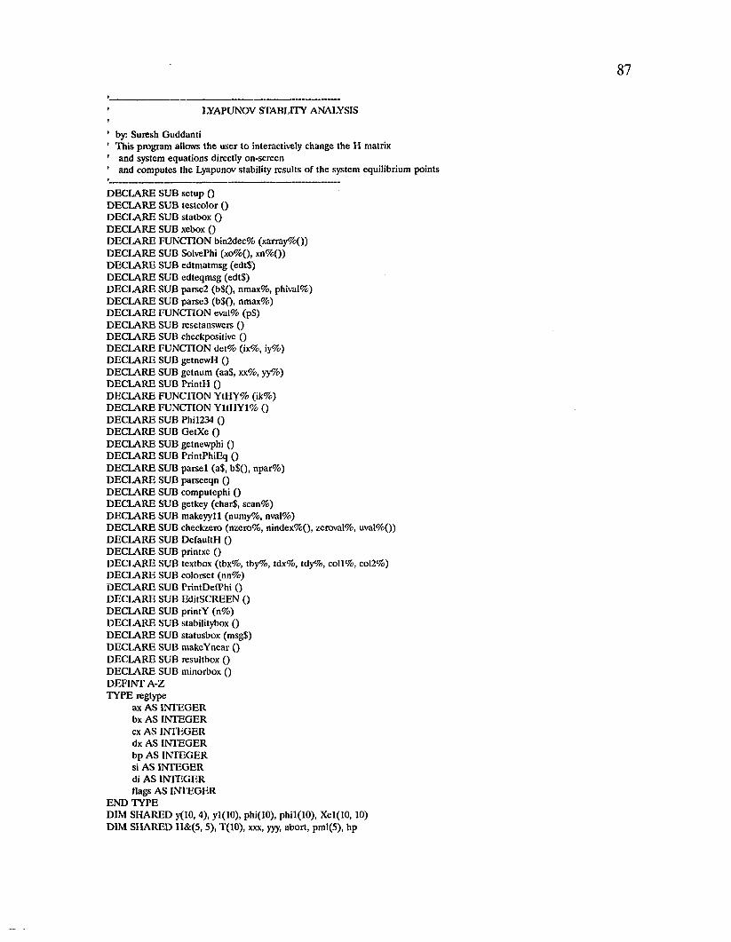
LYAPUNOV STABLITY ANALYSIS

by: Suresh GuddantiThis program allows the user to interactively change the II matrix and system equations directly on-screenand computes the Lyapunov stability results of the system equilibrium points

DECLARE SUB setup ()DECLARE SUB testcolor ()DECLARE SUB statbox ()DECLARE SUB xebox ()DECLARE FUNCTION bin2dec% (xarray%())DECLARE SUB SolvePhi (xo%(), xn%())DECLARE SUB edtmatmsg (edt$)DECLARE SUB edteqmsg (edt$)DECLARE SUB parse2 (b$(), nmax%, phival%)DECLARE SUB parse3 (b$(), nmax%)DECLARE FUNCTION eval% (p$)DECLARE SUB resetanswers ()DECLARE SUB checkpositive ()DECLARE FUNCTION det% (ix%, iy%)DECLARE SUB getnewH ()DECLARE SUB getnum (aa$, xx%, yy%)DECLARE SUB PrintH ()DECLARE FUNCTION YtHY% (ik%)DECLARE FUNCTION YltHYl% ()DECLARE SUB Phil234 ()DECLARE SUB GetXe ()DECLARE SUB getnewphi ()DECLARE SUB PrintPhiEq ()DECLARE SUB parsel (a$, b$(), npar%)DECLARE SUB parseeqn ()DECLARE SUB computephi ()DECLARE SUB getkey (char$, scan%)DECLARE SUB makeyyll (numy%, nval%)DECLARE SUB checkzero (nzero%, nindex%(), zeroval%, uval%()) DECLARE SUB DefaultH ()DECLARE SUB printxc ()DECLARE SUB textbox (tbx%, tby%, tdx%, tdy%, coll%, col2%) DECLARE SUB colorset (nn%)DECLARE SUB PrintDefPhi ()DECLARE SUB EditSCREEN ()DECLARE SUB printY (n%)DECLARE SUB stabilitybox ()DECLARE SUB statusbox (msg$)DECLARE SUB makeYnear ()DECLARE SUB resultbox ()DECLARE SUB minorbox ()DEFINT A-Z TYPE regtype

ax AS INTEGER bx AS INTEGER cx AS INTEGER dx AS INTEGER bp AS INTEGER si AS INTEGER di AS INTEGER flags AS INTEGER

END TYPEDIM SHARED y(10, 4), yl(10), phi(10), phil(10), Xel(10, 10)DIM SHARED H&(5, 5), T(10), xxx, yyy, abort, pml(S), hp

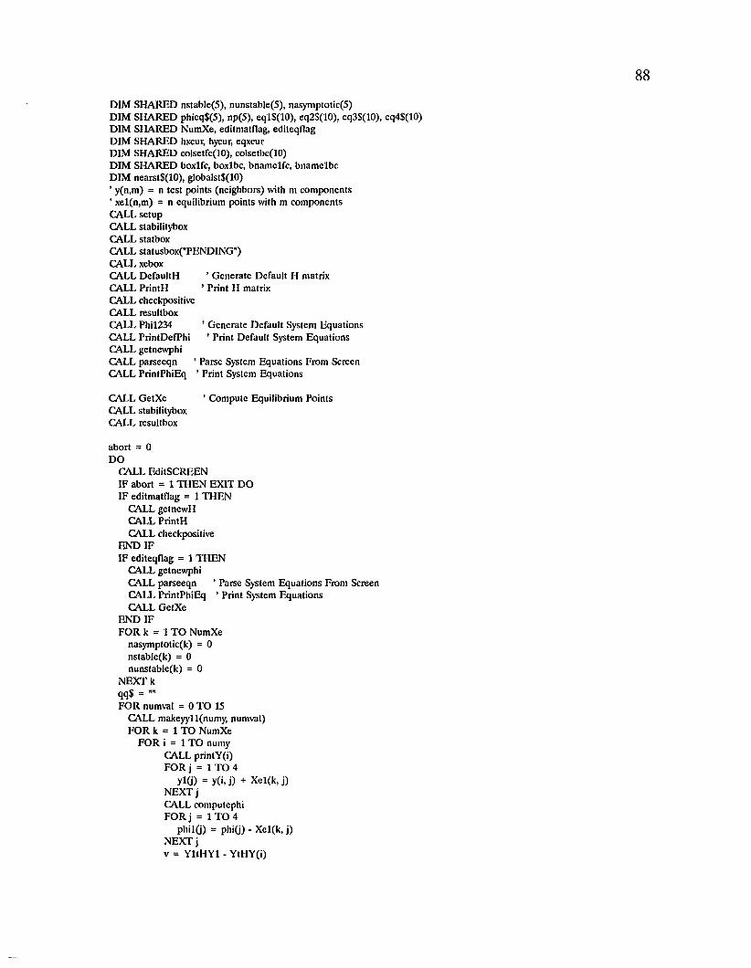
DIM SHARED nstable(5), nunstable(5), nasymptotic(5)DIM SHARED phieq$(5), np(5), eql$(10), eq2$(10), eq3$(10), eq4$(10) DIM SHARED NumXe, editmatflag, editcqflag DIM SHARED hxcur, hycur, eqxcur DIM SHARED colsetfc(lO), colsetbc(lO)DIM SHARED boxlfc, boxlbc, bnamelfc, bnamelbc DIM nearst$(10), globalst$(10)’ y(n,m) = n test points (neighbors) with m components ’ xel(n,m) = n equilibrium points with m componentsCALL setupCALL stabilityboxCALL statboxCALL statusbox("PENDING")CALL xeboxCALL DefaultH ’ Generate Default H matrixCALL PrintH ’ Print H matrixCALL checkpositiveCALL resultboxCALL Phil234 ’ Generate Default System EquationsCALL PrintDefPhi ’ Print Default System EquationsCALL getnewphiCALL parseeqn ’ Parse System Equations From ScreenCALL PrintPhiEq 1' Print System Equations

CALL GetXe ’ Compute Equilibrium PointsCALL stabilityboxCALL resultbox

abort = 0DO

CALL EditSCREEN IF abort = 1 THEN EXIT DO IF editmatflag = 1 THEN

CALL getnewH CALL PrintH CALL checkpositive

END IFIF editeqflag = 1 THEN

CALL getnewphiCALL parseeqn ’ Parse System Equations From Screen CALL PrintPhiEq ’ Print System Equations CALL GetXe

END IFFOR k = 1 TO NumXe

nasymptotic(k) = 0 nstable(k) = 0 nunstable(k) = 0

NEXT k qq$ = ""FOR numval = 0 TO 15

CALL makeyyll(numy, numval)FOR k = 1 TO NumXe

FOR i = 1 TO numy CALL printY(i)FOR j = 1 TO 4

y l© = y(i. j) + Xel(k, j)NEXT jCALL computephi FOR j = 1 TO 4

phil(j) = phi© - Xel(k, j)NEXT jv = Y ltH Yl - YtHY(i)

LOCATE 3 + k qq$ = qqS + INKEYS IF qq$ < > "" THEN

statusbox ("ABORTED")GOTO 100

END IF colorset (2)LOCATE, , 0 SELECT CASE v

CASE IS < 0 ’ Asymptotic Stablenasymptotic(k) = nasyniptotic(k) + 1 LOCATE , 44PRINT USING ”# # # # " ; nasymptotic(k)

CASE IS = 0 ’ Stablenstable(k) = nstable(k) + 1 LOCATE , 22PRINT USING "####"; nstable(k)

CASE IS > 0 ’ Unstablenunstable(k) = nunstable(k) + 1 LOCATE , 32PRINT USING "####"; nunstable(k)

CASE ELSE BEEP: BEEP: BEEP

END SELECT IF numval = 0 THEN

IF nasymptotic(k) > 0 THEN nearstS(k) = "Asymptotic" IF nstable(k) > 0 THEN nearstS(k) = "Stable "IF nunstable(k) > 0 THEN nearst$(k) = "Unstable " LOCATE 3 + k, 56: colorset (2): PRINT ncaist$(k)

ELSEIF nasymptotic(k) > 0 THEN globalstS(k) = ’Asymptotic" IF nstable(k) > 0 THEN globalstS(k) = "Stable "IF nunstable(k) > 0 THEN globalstS(k) = "Unstable " LOCATE 3 + k, 67: colorset (2): PRINT globalst$(k)

END IF NEXT i

NEXT kIF numval = 0 THEN

ntmp = 0FOR k = 1 TO NumXe

IF nearst$(k) = "Unstable " THEN ntmp = ntmp + 1 NEXT kIF ntmp = NumXe THEN EXIT FOR

END IF NEXT numval

statusbox ("COMPLETE")100 LOOP PALETTE COLOR 7, 0 CLSSOUND 2000, 4PRINT "PROGRAM TERMINATED"END

FUNCTION bin2dec (xarray()) dxval = 0 FOR i = 1 TO 4

dxval = dxval + xarray(i) * 2 * (i - 1)NEXT i

90

bin2dec = dxval END FUNCTION

SUB checkpositive hp = 1pm!(l) = H&(1, 1)IF pm!(l) < = 0 THEN hp = -1pm!(2) = H& (1,1) * II&(2, 2) - H&(1, 2) * H&(2, 1)IF pm!(2) < = 0 THEN hp = -1pm!(3) = H&(1, 1) * (H&(2, 2) * H&(3, 3) - H&(2, 3) * H&(3, 2)) - H&(1, 2) * (H & (2,1) * H&(3, 3) - H& (3,1) * H&(2, 3)) + H&(1, 3) * (H&(2, 1) * H&(3, 2) - H&(2, 2) * H&(3, 1))IF pm!(3) < = 0 THEN hp = -1

dl& = II&(2, 2) * det(3, 4) - H&(2, 3) * det(2, 4) + II&(2,4) * det(2, 3)d2& = H&(2, 1) * det(3, 4) - H&(2, 3) * det(l, 4) + II&(2, 4) * det(l, 3)d3& = H&(2, 1) * det(2, 4) - II&(2, 2) * det(l, 4) + H&(2, 4) * det(l, 2)d4& = H&(2, 1) * det(2, 3) - H&(2, 2) * det(l, 3) + II&(2, 3) * det(l, 2)pm!(4) = H&(1, 1) * dl& - H&(1, 2) * d2& + II&(1, 3) * d3& - H&(1, 4) * d4&IF pm!(4) < = 0 THEN hp = -1CALL minorboxLOCATE 22, 2: PRINT pm!(l)LOCATE , 2: PRINT pm!(2);LOCATE 22, 12: PRINT pm!(3)LOCATE , 12: PRINT pm!(4);LOCATE 20, 2 COLOR,2 IF hp > 0 THEN

PRINT "POSITIVE DEFINITE"ELSE

PRINT "NOT POSITIVE DEFINITE"END IF END SUB

SUB checkzero (nzero, nindex(), zeroval, uval()) nzero = 0 FOR i = 1 TO 4

IF uval(i) = zeroval THEN nzero = nzero + 1 nindex(nzero) = i

END IF NEXT i END SUB

SUB colorset (nn)COLOR colsetfc(nn), colsetbc(nn)END SUB

SUB computephiCALL parsel(phieq$(l), eql$(), np(l))CALL parse3(eql$(), np(l))CALL parse2(eql$(), np(l), phival) phi(l) = phival

CALL parsel(phieq$(2), eq2$(), np(2))CALL parse3(eq2$(), np(2))CALL parse2(eq2$(), np(2), phival) phi(2) = phival


91


END SUB

SUB DefaultH

’ Default H matrix

H& (1,1) = 10 H&(1, 2) = -2 H&(1, 3) = 0 H&(1, 4) = 0

H & (2,1) = -2 H&(2, 2) = 20 H&(2, 3) = -15 H&(2, 4) = 20

H&(3, 1) = 0 H&(3, 2) = -15 H&(3, 3) = 30 H&(3, 4) = -20

H&(4, 1) = 0 H&(4, 2) = 20 H&(4, 3) = -20 H&(4, 4) = 40

END SUB

FUNCTION det (ix, iy)det = H&(4, iy) * H&(3, ix) - H&(4, ix) * H&(3, iy) END FUNCTION

SUB EditSCREEN yy = hycur xx = hxcur editmatflag = 0 editeqflag = 0 edtmatmsg ("Editing")LOCATE yy, xx, 1 scan = 0WHILE scan < > 28

CALL getkey(a$, scan)COLOR 11,1 SELECT CASE scan

CASE IS = 15 IF xx > eqxcur - 2 THEN

xx = 2edtmatmsg ("Editing”) edteqmsg (" ")

ELSE xx = eqxcur edtmatmsg (" ")edteqmsg ("Editing")

END IF CASE IS = 77

IF xx < 80 THEN xx = xx + 1 IF xx > eqxcur THEN

edtmatmsg (" ")edteqmsg ("Editing")

END IF CASE IS = 75

IF xx > 2 THEN xx = xx - 1 IF xx < eqxcur THEN

edtmatmsg ("Editing”) edteqmsg (" ")

END IF CASE IS = 72

yy = y y -1IF yy < 15 THEN yy = 15

CASE IS = 80 yy = yy + 1IF yy > 18 THEN yy = 18

CASE IS = 28XXX = XX

yyy = yy c a s e i s = 1

abort = 1 EXIT SUB

CASE IS = 46 testcolor

CASE ELSE IF xx < eqxcur - 1 AND editmatflag = 0 THEN

editmatflag = 1 CALL resetanswers

END IFIF xx > eqxcur -1 AND editeqflag = 0 THEN

editeqflag = 1 CALL resetanswers

END IFLOCATE yy, xx, 1 colorset (2)COLOR 11 PRINT a$;XX = XX + 1

END SELECT LOCATE yy, xx, 1

WEND

END SUB

SUB edteqmsg (edt$)LOCATE hycur - 1, eqxcur + 1, 0: colorset (1) PRINT edt$END SUB

SUB edtmatmsg (edt$)LOCATE hycur - 1, hxcur + 1, 0: colorset (1) PRINT edt$END SUB

FUNCTION eval (p$)IF MID$(p$, 1, 1) = "z" THEN

eval = yl(VAL(MID$(p$, 2)))ELSE

eval = VAL(p$)END IFEND FUNCTION

SUB getkey (char$, scan)DIM inregs AS regtype, outregs AS regtype outregs.flags = 64 WHILE outregs.flags AND 64

inregs.ax = &H100CALL interrupt(&H16, inregs, outregs)

WEND inregs.ax = 0CALL interrupt(&H16, inregs, outregs)scan = outregs.ax \ 255char$ = CHR$((outregs.ax - scan) MOD 255)IF char$ > = "0" AND char$ < = "9" THEN scan END SUB

SUB getnewH

’ Obtain H matrix from Screen cl = 0yy = hycur - 1 xx = 1FOR i = 1 TO 4 yy = yy + 1 xx = 1FOR j = 1 T 0 4

nn = 0CALL getnum(aa$, xx, yy)H&(i, j) = VAL(aa$)

NEXT j NEXT i COLOR,0 LOCATE, , 0 END SUB

SUB getnewphi yy = hycur - 1 FOR i = 1 TO 4

yy = yy + 1 xx = 30 phieq$(i) = ""WHILE xx < 80

CALL getnum(aa$, xx, yy) phieq$(i) = phieq$(i) + aa$

WEND NEXT i

END SUB

SUB getnum (aa$, xx, yy) aa$ = "" nn = 32WHILE nn = 32

nn = SCREEN(yy, xx) xx = xx + 1IF xx > = 80 THEN EXIT SUB

WENDXX = XX - 1

WHILE nn < > 32 nn = SCREEN(yy, xx) aa$ = aa$ + CHR$(nn) xx = xx + 1IF xx = 80 THEN EXIT SUB

WEND

94

END SUB

SUB GetXeDIM Xold(5), Xnew(5), resultof(30)’ COMPUTE EQUILIBRIUM POINTS NumXe = 1 CALL xebox colorset (2)LOCATE 4, 3, 1: PRINT "Computing...";LOCATE, , 0 NumXe = 0 FOR i = 0 TO 15

FOR j = 1 T 0 4Xold(j) = SGN(2 " G ' l ) AND i)

NEXT jCALL SolvePhi(Xold(), Xnew()) ddold = bin2dec(Xold()) ddnew = bin2dec(Xnew())IF ddold = ddnew THEN

NumXe = NumXe + 1 FOR j = 1 T O 4

Xel(NumXe, j) = Xnew(j)NEXT j

ELSEresultof(ddold) = ddnew

END IF NEXT i CALL xebox CALL printxe CALL stabilitybox CALL resultbox END SUB

SUB makeYnear

’ generate Immediate Neighborhood points

FOR i = 1 TO 4FOR j = 1 TO 10

y(j. >) = oNEXT j

NEXT i y(l, 1) = -1 y(2, 2) = -1 y(3, 3) = -1 y(4, 4) = -1y(s. 4) = i y(6> 3) = l y(7 ,2) = ly (8 ,1) = 1 END SUB

SUB makeyyll (numy, nval)DIM nindex(5), u(5), uval(5)IF nval = 0 THEN ’ Test only nearest Neighbors

CALL makeYnear numy = 8 EXIT SUB

END IFFOR i = 1 TO 4

uval(i) = SGN(2 " (i - 1) AND nval) y(l, i) = uval(i)

95

y(2, i) = -uval(i)NEXT i numy = 2

zeroval = 0CALL checkzero(nzero, nindex(), zeroval, uval())IF nzero < > 0 THEN

FOR i = 1 TO 4 u(i) = uval(i)

NEXT iFOR i = 1 TO (2 * nzero) - 1

FOR j = 1 TO nzerou(nindexG')) = -1 * SGN(2 A (j - 1) AND i)

NEXT j numy = numy + 1 FOR j = 1 T O 4

y(numy, j) = u©NEXT j NEXT i

END IF END SUB

SUB minorboxCALL textbox(2, 21, 20, 3, 1, 2)LOCATE 21, 2: colorset (1): PRINT " Principal Minors" colorset (2)END SUB

SUB parsel (a$, b$(), npar) nb = 0 i = 0 bb$ = ""WHILE bb$ < > " = "

i = i + 1bb$ = MID$(a$, i, 1)

WEND i = i + 1WHILE i < = LEN(a$)

aa$ = MID$(a$, i, 1)SELECT CASE aa$CASE IS =

nb = nb + 1 b$(nb) =

CASE IS = "+" nb = nb + 1 b$(nb) = " + "

CASE IS =nb = nb + 1 b$(nb) =

CASE IS = ""CASE IS = ""CASE ELSE

nb = nb + 1b$(nb) = *"bb$ = MID$(a$, i, 1)WHILE (bb$ < > " ") AND (i < = LEN(a$)) AND bb$ < > "•" AND bb$ < > " + " AND bb$ < >

b$(nb) = b$(nb) + bb$ i = i + 1bb$ = MID$(a$, i, 1)

WEND i = i - 1

END SELECT

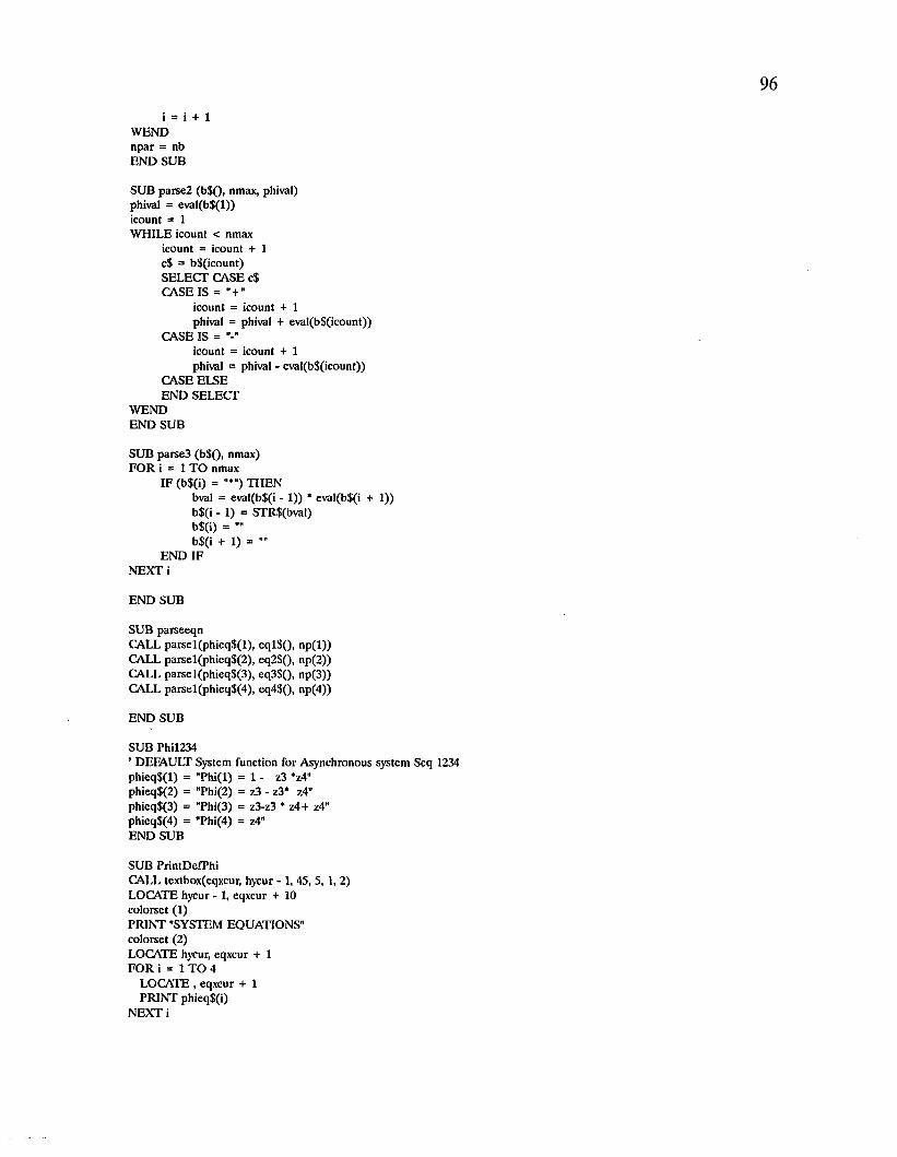
i = i + 1 WEND npar = nb END SUB

SUB parse2 (b$(), nmax, phival) phival = eval(b$(l)) icount = 1WHILE icount < nmax

icount = icount + 1 c$ = b$(icount)SELECT CASE c$CASE IS = " + "

icount = icount + 1phival = phival + evaI(b$(icount))

CASE IS =icount = icount + 1phival = phival - eval(b$(icount))

CASE ELSE END SELECT

WEND END SUB

SUB parse3 (b$(), nmax)FOR i = 1 TO nmax

IF (b$(i) = "»") THENbval = eval(b$(i -1 )) * eval(b$(i + 1)) b$(i - 1) = STR$(bval) b$(i) = "" b$(i + 1) = ',B

END IF NEXT i

END SUB

SUB parseeqnCALL parsel(phieq$(l), eql$(), np(l))CALL parsel(phieq$(2), eq2$(), np(2))CALL parsel(phieq$(3), eq3$(), np(3))CALL parsel(phieq$(4), eq4$(), np(4))

END SUB

SUB Phil234’ DEFAULT System function for Asynchronous system Seq 1234phieq$(l) = "Phi(l) = 1 - z3 *z4"phieq$(2) = flPhi(2) = z3 - z3* z4"phieq$(3) = "Phi(3) = z3-z3 * z4+ z4"phieq$(4) = ”Phi(4) = z4"END SUB

SUB PrintDefPhiCALL textbox(cqxcur, hycur - 1, 45, 5 ,1 , 2)LOCATE hycur - 1, eqxcur + 10 colorset (1)PRINT "SYSTEM EQUATIONS" colorset (2)LOCATE hycur, eqxcur + 1 FOR i = 1 TO 4

LOCATE , eqxcur + 1 PRINT phieq$(i)

NEXT i

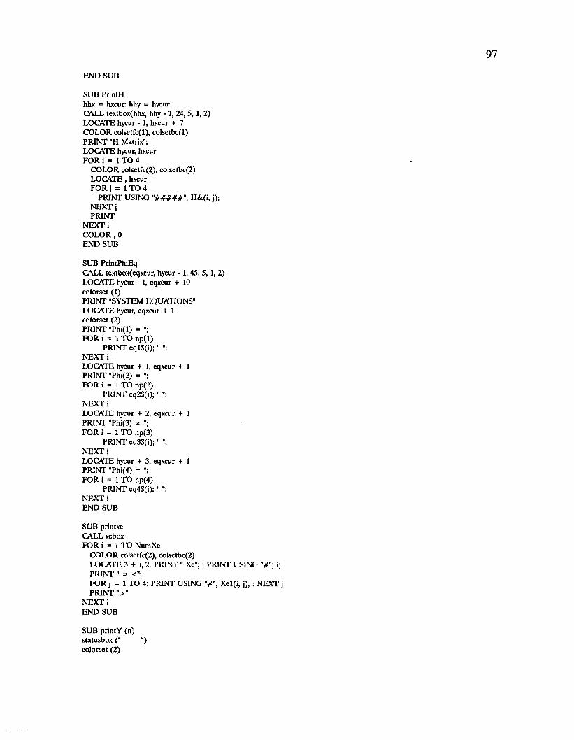
97

END SUB

SUB PrintHhhx = hxcur: hhy = hycurCALL textbox(hhx, hhy - 1, 24, 5 ,1 , 2)LOCATE hycur - 1, hxcur + 7 COLOR colsetfc(l), colsetbc(l)PRINT "H Matrix";LOCATE hycur, hxcur FOR i = 1 TO 4

COLOR colsetfc(2), colsetbc(2)LOCATE, hxcur FOR j = 1 T O 4

PRINT USING ”# # # # # ”; H&(i, j);NEXT j PRINT

NEXT i COLOR,0 END SUB

SUB PrintPhiEqCALL textbox(eqxcur, hycur - 1, 45, 5,1, 2)LOCATE hycur - 1, eqxcur + 10 colorset (1)PRINT "SYSTEM EQUATIONS"LOCATE hycur, eqxcur + 1 colorset (2)PRINT "Phi(l) = ";FOR i = 1 TO np(l)

PRINT eql$(i); "NEXT iLOCATE hycur + 1, eqxcur + 1 PRINT "Phi(2) =FOR i = 1 TO np(2)

PRINT eq2$(i); ”NEXT iLOCATE hycur + 2, eqxcur + 1 PRINT "Phi(3) = ";FOR i = 1 TO np(3)

PRINT eq3$(i); " ";NEXT iLOCATE hycur + 3, eqxcur + 1 PRINT ”Phi(4) =FOR i = 1 TO np(4)

PRINT eq4$(i); "NEXT i END SUB

SUB printxe CALL xebox FOR i = 1 TO NumXe

COLOR colsetfc(2), colsetbc(2)LOCATE 3 + i, 2: PRINT " Xe";: PRINT USING "#"; i; PRINT " = <";FOR j = 1 TO 4: PRINT USING Xel(i, j); : NEXT j PRINT ">"

NEXT i END SUB

SUB printY (n) statusbox (" ")colorset (2)

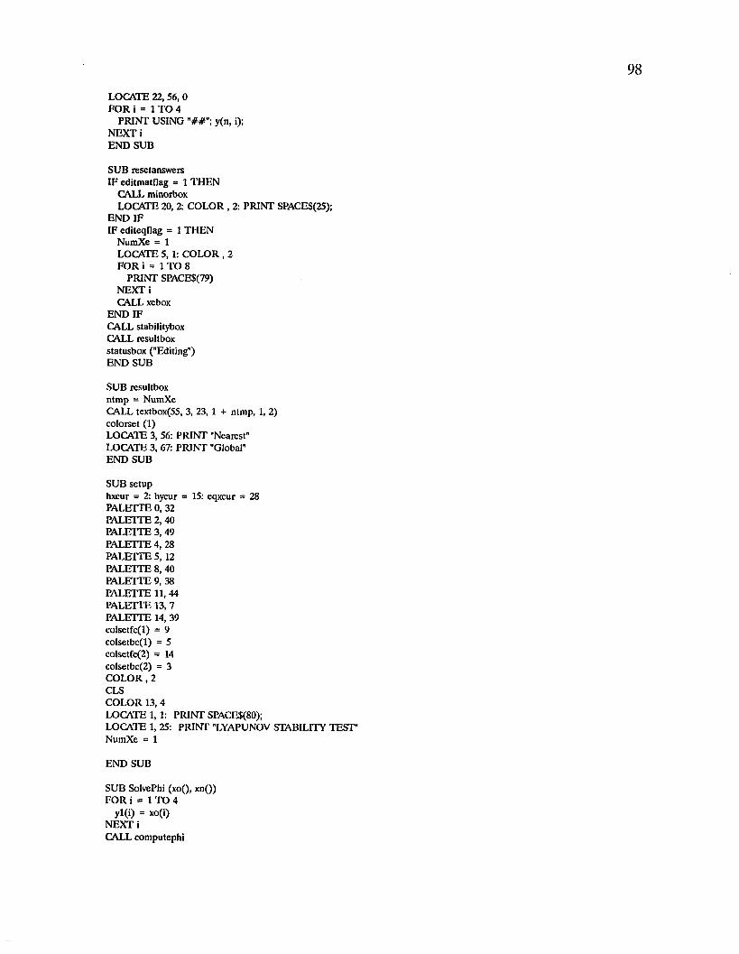
LOCATE 22, 56, 0 FOR i = 1 TO 4

PRINT USING y(n, i);NEXT i END SUB

SUB resetanswers IF editmatflag = 1 THEN

CALL minorboxLOCATE 20, 2: COLOR , 2: PRINT SPACE$(25);

END IFIF editeqflag = 1 THEN

NumXe = 1LOCATE 5,1: COLOR , 2 FOR i = 1 TO 8

PRINT SPACE$(79)NEXT i CALL xebox

END IFCALL stabilitybox CALL resultbox statusbox ("Editing")END SUB

SUB resultbox ntmp = NumXeCALL textbox(55, 3, 23, 1 + ntmp, 1, 2) colorset (1)LOCATE 3, 56: PRINT "Nearest"LOCATE 3, 67: PRINT "Global"END SUB

SUB setuphxcur = 2: hycur = 15: eqxcur = 28PALETTE 0, 32PALETTE 2, 40PALETTE 3, 49PALETTE 4, 28PALFITE 5, 12PALETTE 8, 40PALETTE 9, 38PALETTE 11, 44PALETTE 13, 7PALETTE 14, 39colsetfc(l) = 9colsctbc(l) = 5colsetfc(2) = 14colsetbc(2) = 3COLOR,2CLSCOLOR 13, 4LOCATE 1, 1: PRINT SPACE$(80);LOCATE 1, 25: PRINT "LYAPUNOV STABILITY TEST" NumXe = 1

END SUB

SUB SolvePhi (xo(), xn())FOR i = 1 TO 4

y i(0 = *>(■)NEXT iCALL computephi

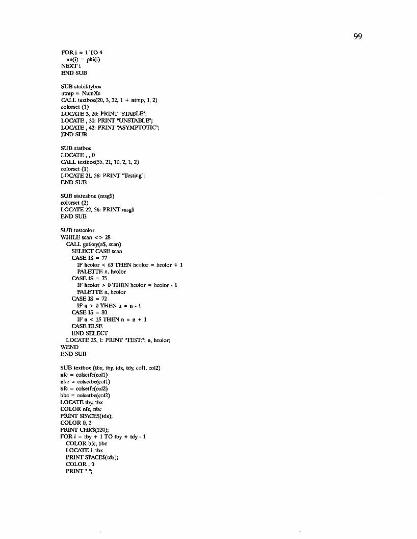
FOR i = 1 TO 4 xn(i) = phi(i)

NEXT i END SUB

SUB stabilitybox ntmp = NumXeCALL textbox(20, 3, 32, 1 + ntmp, 1, 2) colorset (1)LOCATE 3, 20: PRINT "STABLE";LOCATE , 30: PRINT "UNSTABLE";LOCATE , 42: PRINT "ASYMPTOTIC";END SUB

SUB statbox LOCATE , , 0CALL textbox(55, 21, 10, 2 ,1 , 2) colorset (1)LOCATE 21, 56: PRINT "Testing";END SUB

SUB statusbox (msg$) colorset (2)LOCATE 22, 56: PRINT msg$END SUB

SUB testcolor WHILE scan < > 28

CALL getkey(a$, scan)SELECT CASE scan CASE IS = 77

IF hcolor < 63 THEN hcolor = hcolor + 1 PALETTE n, hcolor

CASE IS = 75 IF hcolor > 0 THEN hcolor = hcolor - 1 PALETTE n, hcolor

CASE IS = 72 IF n > 0 THEN n = n - 1

CASE IS = 80 IF n < 15 THEN n = n + 1

CASE ELSE END SELECT

LOCATE 25, 1: PRINT "TEST:"; n, hcolor; WEND END SUB

SUB textbox (tbx, tby, tdx, tdy, coll, col2)nfc = colsetfc(coll)nbc = colsetbc(coll)bfc = colsetfc(col2)bbc = colsetbc(col2)LOCATE tby, tbx COLOR nfc, nbc PRINT SPACES(tdx);COLOR 0, 2 PRINT CHR$(220);FOR i = tby + 1 TO tby + tdy - 1

COLOR bfc, bbc LOCATE i, tbx PRINT SPACE$(tdx);COLOR,0 PRINT"";

NEXT i COLOR 0, 2LOCATE tby + tdy, tbx + 1 PRINT STRING$(tdx, 223);END SUB

SUB xebox ntmp = NumXeCALL textbox(2, 3 ,16 ,1 + ntmp, 1, 2) COLOR colsetfc(l), colsetbc(l) LOCATE 3, 2: PRINT "Equilibrium Pts"; END SUB

FUNCTION Y ltH Yl

’ Compute ylthyl

zz = 0FOR i = 1 TO 4

T(i) = 0 FOR j = 1 T O 4

T(i) = T(i) + ph il© * H&(j> i) NEXT jzz = zz + T(i) * phil(i)

NEXT i Y ltH Y l = zz END FUNCTON

FUNCnON YtHY (ik)

’ compute YtHY

zz = 0FOR i = 1 TO 4

T(i) = 0 FOR j = 1 T O 4

T(i) = T(i) + y(ik, j) * H&(j, i) NEXT jzz = zz + T(i) * y(ik, i)

NEXT i YtHY = zz END FUNCTION

VITA

Suresh Guddanti was bora on September 25, 1960, in Kurnool located in

Andhra Pradesh state of India, son of G. Sri Krishna Murty and G. Manikyam. He

attended high school at Atomic Energy Central School, Bombay, India. Mr.

Guddanti has graduated First Class with Distinction with a Bachelor of Engineering

in Mechanical Engineering.

Mr. Guddanti has worked as a Research Engineer for Larsen & Toubro

Limited, Bombay, for two years. He obtained his Masters Degree in Mechanical

Engineering at Louisiana State University in December 1987.

101

DOCTORAL EXAMINATION AND DISSERTATION REPORT

Candidate: Suresh G uddanti

Major Field: M ech an ica l E n g in e e r in g

Title of Dissertation: A N eu ra l Network T ruth M aintenance System

Approved:

M ajor Professor and la irm ai

D ean of the Graduate School

EXAMINING COMMITTEE:

'£ J L

Date of Examination:

4 / 2 6 / 9 1

Documents

A Neural Network Truth Maintenance System