Pergamon S0952-1976(96)00006-1

EngngApplic. Artif. lntell. Vol. 9, No. 2, pp. 153-161, 1996 Copyright t~) 1996 Elsevier Science Ltd

Printed in Great Britain. All tights reserved 0952-1976196 $15.00 + 0.00

Contributed Paper

A Neuro-Expert System for the Prediction of Software Metrics

J. S. MERTOGUNO Binghamton University, U.S.A.

R. PAUL Office of the Under Secretary of Defense, U.S.A.

N. G. BOURBAKIS Binghamton University, U.S.A.

C. V. RAMAMOORTHY University of California at Berkeley, U.S.A.

(Received December 1994; in revised form December 1995)

This paper deals with the design and modeling of a neuro-expert (NE) system for the prediction of software metrics. The NE consists of two neural networks and an expert system with fuzzy reasoning in order to achieve a better evaluation of software metrics. More specifically, the importance of using both neural networks and an expert system is to combine the adaptive nature of neural networks on different sets of data, with the high-level reasoning provided by the expert system, for a better overall evaluation. In this paper the first stage modeling of the NE system is presented. Copyright (~ 1996 Elsevier Science Ltd

Keywords: Software metrics, expert systems, neural networks, software interfaces, fuzzy reasoning.

1. INTRODUCTION

Successful project management requires the bench- marking and tracking of projects. In order to assess a project's performance, metrics are generated, so that a project can be analyzed quantitatively. ~-3 Large soft- ware projects are no exception, and in fact the com- plexity and scale of software projects can be daunting without some quantitative measures. 2 Once the metrics have been gathered the problem of analysis must be addressed. This paper describes an approach to pro- cessing the U.S. Army Software Testing and Evaluation Program (STEP) software metrics. 4

Classical analytical techniques have been applied to metrics in the past, and can provide information about metric value distributions and correlation. 2'3 Neural networks are tools which have been widely applied to analyzing data, and are useful in environments where

Correspondence should be sent to: Professor N. G. Bourbakis, Depar tment of Electrical Engineering, T. J. Watson School of Applied Sciences, A A A I Lab, SUNY--Binghamton , Binghamton, NY 13902-6000, U.S.A.

correlations among variables are difficult to compute due to the complexity of the environment, and where there are large amounts of data to train the network. 5 The backpropagation neural-network model is a method of characterizing a possibly noisy dataset, and interpolating new data based on that characterization)

This paper describes an approach using a backpropa- gation neural network and a fuzzy rule-based system for assisting in the analysis and application of the software metric information. More specifically, the paper describes the expert-system extension of the neural-network concept to a working system using a real metric data format. The STEP Neural Network Interface (SNNI) uses past project STEP metric data- sets to train a backpropagation neural network to predict the final software project status of an uncom- pleted project. The expert (rule-based) system exten- sion of SNNI gives a second prediction and an interpre- tation of the metrics. The results from the neural network and the expert system can be used to intervali- date each other. The use of fuzzy logic in the inference engine of SNNI helps to reduce the number of rules needed.

153

154 J .S. MERTOGUNO et al. : SOFTWARE METRICS

M~ric Name milcsa~ fast available Cost 0 ~ e 0 *CRU 1 +Em,irotmaeat N/A

Tr,~ility

Sta~ay Design 2

Stability ~ta~xity 2 Bl~,,~ith of 2 T~ing

D~th of 2 r ~ i ~

Fatdt Prafile 3 Reliability 3

* "Computer Resource Utilization" + F_avirmu~ metric, a non-hurtle quantity, is not used

Fig. 1. Summary of the STEP metrics.

2. PROJECTION OF PROJECT'S METRICS

The STEP program has adopted a set of metrics based on past software metrics analysis. 4 There are 12 metrics, each of which has several numeric compo- nents. Figure 1 shows a list of the metric types. These metrics are described further in the database interface description below.

Milestones in a project refer to events marking a change in the phase of the project. This system considers a project 's progress to be one of five mile- stones. Milestones are used to quantize a project 's progress into stages that can reasonably be compared. Figure 1 shows the milestone at which each metric is first available.

3. A NEW SNNI DESIGN

The global design of a new SNNI version is shown in Fig. 2. It consists of five units. These units are: the User Interface, the Database, the Neural Network 1, the Neural Network 2, and the Expert System. As can be seen in Fig. 2, the raw data is handled by the first-stage neural network (NN1). This first-stage neural network provides inputs for both the second-stage neural network (NN2) and the expert system.

User L

Fig. 2. Global design of the SNNI.

3.1. The user interface (UI)

The user interface module provides the user with control over the operation of other modules in the SNNI. It has a screen to display the output of the expert system, the NN1, the NN2 and messages about the states of the operations. The user interface has connec- tions to almost all of the SNNI units (except for the clause generator). The UI unit provides for interaction between the user and the SNNI.

3.2. The database interface

The most complex part of the SNNI system is the interface between the database and the neuro-expert system. The metric data cannot be fed directly to the neural network. The metric database available is a set of text files, one file per metric. Each file has one line per metric checkpoint, and most metrics are gathered on a monthly schedule. In order to be able to accommodate the data into the neural network input, another set of data has to be extracted from the metric data set.

The database interface generates one file for each project. This file has five records, one for each mile- stone. Each record has 179 fields, representing the pre- processed metric data.

The design of SNNI includes conceptually five neural networks, one for projection from each milestone. These neural networks have different numbers of input features, depending to the number of metrics available at that particular milestone. For unavailable data, a value of zero is given.

Additional data is needed to extract the new data set from the original data set, which is the list of the milestone dates. This is not directly available from the STEP metric database at this time.

The output of the neural network should be a rela- tively simple quantity in order to be of more immediate use than the entire metric set. The simplest method of achieving it is a good/bad dichotomy classification of the project, as discussed in Ref. 6. If possible, it is desired to get more information than this, but there is no need to go beyond a certain point of detail since the network only approximates based on past experience. It cannot reasonably be expected to get a fully detailed projection of all metrics. The output of SNNI is chosen to be:

(1) a projection of the schedule deviation; (2) a projection of the cost deviation.

These two pieces of information will be able to indicate the global characteristics of the project. They will give some indication to the user of the degree of success, rather than just a binary success/failure. These output parameters are calculated from the available cost and schedule metrics.

3.3. Neural network 1 (NN1)

The neural network 1 has a number of inputs equal to the number of parameters in the entire software metric.

J. S. MERTOGUNO et al. : SOFFWARE METRICS 155

The output of the NN1 will be directly fed to both NN2 and the clause generator. NN1 has a small number of outputs. Each output corresponds to an initial clause to be created by the clause generator. The output of NN1 will be the goodness values extracted from the metrics (one for each metric), and the others are some (one or two) important parameters extracted from each metric. These important parameters are yet to be determined by the experts in this field.

In front of this NN1 there is an interface that trans- forms raw data into a meaningful set of data for the input of NN1. This interface is the result of the previous phase of the work on SNNI. 7

3.4. Neural network 2

The neural network 2 (NN2) takes all the NN1 outputs as input. NN2 draws ammoverall prediction of the project as its final output(s). The outputs of NN2 are still to be defined by the expert. One of the outputs will be the overall goodness value of the project being evaluated. NN2 is not the only unit that produces final interpretations of the evaluated project; the expert system as a part of SNNI also produces final outputs. If there is any conflict between the final conclusions produced by NN2 and those of the expert system, the judgment is left to the user, to draw a final conclusion based on the results from both NN2 and the expert system.

In order for a good performance to be achieved, the NN1-NN2 path of the SNNI needs to be trained with an appropriate set of data. In training, the NN1-NN2 can be considered as a single multilayer neural network, and trained by using the well-known backpro- pagation method. A simple algorithm is needed to maintain the output values of the NN1 (in the range of 0 to 9) and a different range for those of NN2. Another method is to train the NN1 and the NN2 nets separ- ately. With this method, a set of intermediate NN1 outputs has to be pre-determined. The latter method has been chosen, due to the easier development, and the separation which makes the NN2 part less sensitive to the type of project, a feature that is well received, since it provides more reuse of the sets of trained weight of NN2.

3.5. The rule-based expert system

The expert system consists of four units (the clause generator, the blackboard, the inference engine and the rule base). The clause generator has as many inputs as the number of neural networks [16 in the first stage of the neural networks (NN1)]. The clause generator produces a clause for every NN1 output. These clauses are statements to be used as the starting point of a sequence of inferences which will be generated by the inference engine in order to come to the final conclu- sion. These clauses (statements) are put in the black- board.

The blackboard is a kind of scratch pad for the

operation of the inference engine. All of the input statements, intermediate statements and the final state- ment (final conclusion) are placed in the blackboard. The inference will constantly read the blackboard until a final conclusion is found. In this case, the inference engine will signal the user interface to get the output from the blackboard.

The inference engine is the main part of the expert system. This unit continuously scans both blackboard and rule-base to find sets of statements and rules that can be fired, until a final conclusion is found. Thus this unit has a direct connection to the blackboard and the rule base. When a set of rules and statements is fired, a new statement is produced, along with its belief mea- sure. Thus, the calculation of the belief measure is also the reponsibility of the inference engine. To evaluate the belief measure, a scheme of knowledge and truth representation is needed. The evaluation of the belief measure in SNNI uses fuzzy logic concepts. The discus- sion about this scheme is carried out later in this paper.

The rule-base is the place where all of the rules (knowledge) of the system are stored. These rules are stored in the form of connected statements and their confidence levels. A confidence level represents the goodness level of the corresponding rule.

4. THE EXPERT SYSTEM FOR SNNI

In order to make SNNI more convincing, an expert system has been added to provide explanations about how the conclusion was made. To provide inputs for the expert system, the neural network of SNNI has to be divided into two sections: the first-level and second- level neural networks. The first-level neural network provides inputs to the expert system and to the second- level neural network, as shown in Fig. 3. The expert system and the second-level neural network provide independent final conclusions to the user. Theoretically these independent conclusions should agree to each other, but there will be a case where the results of expert system and the second-stage neural network partially (in rare cases totally) disagree. In this case it is up to the user to judge which conclusion is more accurate. The belief measure in the expert system and the output of the neural network will be good indica- tions by which to judge the conclusions. Note that the

Neural Network- l [ - - cl._ Bl. kbo d I

Generator

] Inference ~ ' Engine

i Expert System I

Fig. 3. Block diagram of SNNI's expert system.

156 J .S. MERTOGUNO et al. : SOFTWARE METRICS

output of the neural networks (both the first and the second stages) are goodness values (in a certain range, for instance 0-1).

4.1. The knowledge model

A rule-based expert system, in general, searches for a corresponding rule for each proposition stored in the blackboard, fires the rules and calculates the belief measure of the resulting proposition. In order for the system to be able to evaluate the belief measure, some kind of knowledge (belief) model has to be defined. Using the fuzzy logic, the belief measure can be eva- luated over a range, using a function to represent the characteristic of the belief value inside the range. The range represents the fuzzy concept, and the characteris- tic function represents the measure of fitness between a certain proposition and the corresponding fuzzy con- cept.

In the fuzzy expert system used here, the characteris- tic function was based on the assumption that the degree of correspondence is normally distributed inside the fuzzy range of the concept. This assumption implies that the most matched condition (point of correspon- dence in a range) occurs when the range of the (compo- nent of the) proposition falls in the middle of the range of the (component of the) rule. The point of correspon- dence is defined as the highest point in the characteris- tic function of a range. This assumption appears to give a good approximation for most of the rules/ propositions, except for two classes of concepts. The first is the class of concepts where the point of corre- spondence of a concept occurs to the extreme right of the range, such as the concept "bigger". The further right the value goes, the better the concept is matched. The second class is the opposite of the first class, where the point of correspondence occurs to the extreme left of the concept's range. In these two classes, one of the boundaries of the range is actually defined as an approximation of infinity which cannot be expressed accurately by a computer, since one is operating in a limited world. In the knowledge model used here, the belief measures for components of propositions are classified into three types, as shown in Fig. 4. These three types are:

• The close-range model, where the point of correspondence falls approximately in the mid- dle of the range, as shown in Fig. 4(a).

• The right open model, where the point of correspondence is located at the extreme right of the range, as shown in Fig. 4(b).

• The left open model, where the point of corre- spondence occurs in the extreme left of the range, as shown in Fig. 4(c).

4.2. Derivation of the characteristic function

As was mentioned above, the distribution of truth in the fuzzy range is approximated by using a normal distribution. This normal distribution model is shown in

(a)

~ _ Mode = - 1

P/L U

L

~ M o d e --- 0

P U

( C ) f Mtxl© = 1

7 1 L PIU

Fig, 4. The belief measure models.

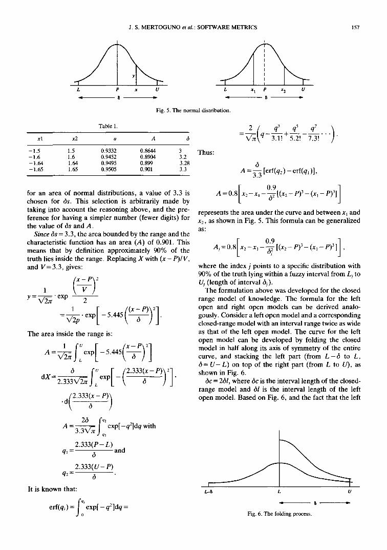
Fig. 5, where it can be seen that there is a fuzzy range with interval length of 6, that starts at L (xl) and ends at U (x2). The characteristic function is symmetrical, with its axis coinciding with the point of correspon- dence (P). The equation for the characteristic function is:

1 y = ~ exp[ - (X2/2)]

and the area under the curve, is:

area = f l ~ exp[-(X2/2)ldX"

The area under the curve from - o0 to U is defined as

a = exp[ - (X2/2)ldX

and the area under the curve between L and U as:

A=f2exp[-(X212)]dX

where

(x - P) L + U X ~ , p = - - - ~ a n d S = U - L .

A scaling parameter V is also defined, such that V = 8/8s = (x-P)/X, where b is the length of the range interval, as was mentioned above, and bs is the length of a chosen standard range interval for a normal distri- bution. The selection of 8s is based on the reasoning that the summation of all the possibilities of truth inside the range should be close to 1. Note that for a fuzzy statement there is always an infinitesimal possibility of the truth lying outside its fuzzy range. From Table 1,

J. S. M E R T O G U N O et al. : S O F T W A R E M E T R I C S 157

L P x U L x I P x 2 U

Fig. 5. The n o r m a l d i s t r ibu t ion .

Tab le 1.

x l x2 a A 6

- 1.5 1.5 0.9332 0.8644 3 - 1.6 1.6 0.9452 0.8904 3.2 - 1.64 1.64 0.9495 0.899 3.28 - 1 . 6 5 1.65 0.9505 0.901 3.3

for an area of normal distributions, a value of 3.3 is chosen for 6s. This selection is arbitrarily made by taking into account the reasoning above, and the pre- ference for having a simpler number (fewer digits) for the value of 6s and A.

Since 6s = 3.3, the area bounded by the range and the characteristic function has an area (A) of 0.901. This means that by definition approximately 90% of the truth lies inside the range. Replacing X with (x - P)/V, and V= 3.3, gives:

1 Y - V ' ~ "exp 2

1

The area inside the range is: [ / x - P \ 2 ] A = ~ - ~ ceXp --5.445~----~) ]

6 (v [ /2.333(x-- dX 2"333X/~JLexp[ - -~ ' p))2] .

. [ 2 . 3 3 3 ( x -

"°k e)) 26

fqz exp[-qZ]dq with a - 3 . 3 ~ |

J ql

2.333(P- L) and q J - 6

2 .333(U- P) q 2 - - 6

It is known that:

erf(qi)=fi 'exp[-q2]dq=

Thus:

2 ( q3 qS q 7 ) =~-~ q - 3 - ~ . 1÷5.2! 7 . 3 ! " " "

6 A = ~-~ [erf(q2) - erf(ql )],

[ 09 ] A =0.8 x2-x,---~-[(x2 - P) 3 - ( x , - p)3]

represents the area under the curve and between x~ and x2, as shown in Fig. 5. This formula can be generalized as"

[ o.9 ] A,=0.8 x 2 - x l - ~ [(x2- P) 3- (x,-e)31 ,

where the index j points to a specific distribution with 90% of the truth lying within a fuzzy interval from Lj to Uj (length of interval dj).

The formulation above was developed for the closed range model of knowledge. The formula for the left open and right open models can be derived analo- gously. Consider a left open model and a corresponding closed-range model with an interval range twice as wide as that of the left open model. The curve for the left open model can be developed by folding the closed model in half along its axis of symmetry of the entire curve, and stacking the left part (from L - 6 to L, 6 = U - L) on top of the right part (from L to U), as shown in Fig. 6.

6c = 261, where 6c is the interval length of the closed- range model and 6l is the interval length of the left open model. Based on Fig. 6, and the fact that the left

Y r--------

L-~ L U

Fig. 6. T h e f o l d i n g process .

158 J .S . M E R T O G U N O et al.: S O F T W A R E METRICS

and right parts of the closed-range model are symmetri- cal, then for the left open model:

y = 2yc = exp --~- ,

with

x - P X = - - and V=

V

6

1.65

(since the left open model is considered as stacked half intervals). Thus:

y = ~ / 2

and:

= 0.8{x2 - xl - - - A/

with P = L.

exp [ - [x - - p\2] 1"362t~-- ) ]'

0.463 } 6~ [(x2-p)3-(x '-p)3] '

By analogy, the equations for the right open model can be formulated as:

[ y = exp - 1 . 3 6 2 t - - - - ~ ) J ,

and

= 0.8{x2 Ai

with P = U.

0.463 } - x, 6~ [ ( x 2 - p ) 3 _ (Xl - P)31 ,

4.3. Calculation of the belief measure

The belief measure is a parameter that approximates how much truth (belief) the result of an inference contains. Naturally, the calculation of the belief meas- ure is a function of the confidence level of the rule, and the cumulative measures of all matching pairs (between components of the statement and components of the rules). Thus, BM =f(ML, CF), where BM is the belief measure of the result, ML is the average matching level of the components, and CF is the confidence level of the rule. In the case where the evaluated statement is an intermediate statement (the result of a previous inference), and not a fact (input statement, BM= 1), the BM of the statement is not unity, and then the belief measure should also be a function of the inter- mediate statement belief measure. Thus, BM =f(BM', ML, CF), where BM' is the belief measure of the intermediate result. CF is a pre-assigned parameter, which its value implies the confidence of the expert in using the corresponding rule. Every rule has its own confidence level. ML is a calculated parameter, where its value depends on the degree of matching between the range of value of the rule and that of the statement, and the size of the intersection area of the rules and of the statement. Thus, ML =f(mlr, mlp), where mlr is

the level of the match according to the intersection area, and mlp is the matching level according to the position of corresponding points of both the rule and the statement.

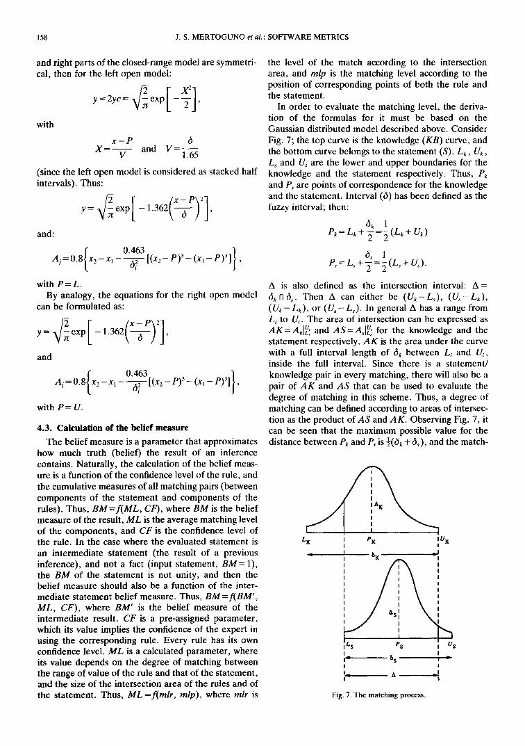
In order to evaluate the matching level, the deriva- tion of the formulas for it must be based on the Gaussian distributed model described above. Consider Fig. 7; the top curve is the knowledge (KB) curve, and the bottom curve belongs to the statement (S). Lk, Uk, Ls and U~ are the lower and upper boundaries for the knowledge and the statement respectively. Thus, Pk and Ps are points of correspondence for the knowledge and the statement. Interval (6) has been defined as the fuzzy interval; then:

6 k 1 P~ = L~+~=~ (L~+ u~)

l P,=L,+~=-~(L,+ U~).

A is also defined as the intersection interval: A= 6k n 6s. Then A can either be (U,~-Ls), (U~--Lk), (Us-Lk) , or (Us-Ls). In general A has a range from Li to Ui. The area of intersection can be expressed as AK=AkJU~ and AS=AsJUL~ for the knowledge and the statement respectively. AK is the area under the curve with a full interval length of 6k between L~ and Ui, inside the full interval. Since there is a statement/ knowledge pair in every matching, there will also be a pair of AK and AS that can be used to evaluate the degree of matching in this scheme. Thus, a degree of matching can be defined according to areas of intersec- tion as the product of AS and AK. Observing Fig. 7, it can be seen that the maximum possible value for the distance between P k and Ps is ½(54 + 6s), and the match-

LK PK I U K I

8 K

/i s

I_ ~ g

Fig. 7. The matching process.

US

KB

ST

J. S. M E R T O G U N O et al. : S O F T W A R E METRICS

= A ~ -o-==-= A

159

(a) (b) (c) (d)

Fig. 8. Four types of matching.

ing level according to the position of the peak (point of correspondence) can be expressed as:

21Pk- P,I mlp 6k + 6s

Having been able to express mlp and mlr mathemati- cally, the total matching level (ML) can be formulated as the geometric mean of mlr and mlp. Thus:

ML = VC-mlr • mlp.

There are also two possible ways to formulate the belief measure. The first way is by using the geometrical mean: BM---~/BM' • ML • CF, and the other is by using fuzzy logic: BM = min(BM', ML, CF). At this point it seems appropriate to use the fuzzy concept. Thus the latter formula will be used. Note that the fuzzy logic can always be used to replace the geometric mean in SNNI. The fuzzy logic has not been used earlier because it is preferable that both (or more) parameters should contribute (geometric mean) to the formulation, rather than choosing one to be used (min or max operator in the fuzzy logic).

Generally, there are four possible types of matching for a closed-range model. These types of matching are shown in Fig. 8(a-d). Additional classes of types of matching (for left open and right open models) are shown in Fig. 9(a-c). Notice that in the left or right

open model, the area of the statement's range outside the intersection interval is included in the calculation of AS.

4.4. Sentence format and the blackboard

The expert system processes sentences by comparing input sentences with knowledge-base sentences, and calculates the belief measures of the resulting sentences. Thus, a sentence and its format has to be defined. Since there are two types of sentences; state- ments and knowledge-base sentences, there are two type of formats:

Statement: P , N , O ,LI , U 1 ,M1 ,L2 , U~ ,M2 ,B M, TF.

Knowledge-base sentence: P,N,O,LI, U1 ,MI ,L2,/-/2 ,M2 # # P,N,O,L1 ,U1 ,M~ ,L2 ,U2 ,M2# . . . . # P,N,O,L1 , U1 ,M l ,L2 ,UE ,M2 > > P,N,O,L1, U1 ,Ml ,L2,/-/2 ,/142 ,CF.

Where P stands for pronoun, N for noun, O for object, Li for lower boundary, Ui for upper boundary, Mi for mode (left open, closed, right open), TF for tracking field, BM for belief measure, and CF for confidence factor. The sign # indicates the 'and' operator, and > separates conditions and conclusion. Notice that the 'or' operator is not supported here, since a sentence

KB

F"

(a) (b)

Fig. 9. Addit ional types of matching.

/L (c)

EAAI9-2-D

160 J.s. MERTOGUNO et al. : SOFFWARE METRICS

with an or operator can be analyzed into two or more simpler sentences without 'or' operators. A tracking field is used to keep track of the fired rules and control the rule firings. The tracking field has the format: A \ B \ C \ D , where A is a flag (0 if completed, and 1 if conditional). B is the number of the last rule which was fired, C is a list (using a point " ." as the delimiter) of unsatisfied conditions, and D is list (with point " ." as delimiter) of fired rules. The use of this tracking field will be discussed later. These formats represent the general form of a statement stored in the blackboard, and a rule in the rule-base.

4.5. The clause generator

The clause generator translates every output of neural network 1 into statements which can be under- stood by the inference engine. These statements will be stored in the blackboard as the initial statements. The clause generator is basically a look-up table which maps every output of NN1 into a specific statement, and translates the output value of NN1 into "Li"s, "Ui"s, and "Mi"s. The translation from the output values into "Li"S, "Ui"s , and "M~"s, follows sets of rules specific for every output of the NN1. Since people have differ- ent interpretation of quality, such as "bad", "OK" and "good", a table of the fuzzy range, along with its interpretation, has to be provided with the data for every qualitative word in the rules. Thus, the clause generator reads the output of the NNI and the fuzzy range table in order to come up with the output sentences.

4.6. The rule-base and the inference engine

All the rules for the expert system are stored in the rule-base in a certain format, as was described in the previous section. The rule base can be accessed by the inference engine to produce statement-rule pairs. This rule-base should contain enough knowledge (extracted from the experts in this area) for the inference engine to make the appropriate decisions. The use of fuzzy logic significantly reduces the number of these rules.

By its nature, there are three types of rules. These types are: simple, conditional (complex), and addi- tional (pseudo-complex). A simple rule has only one condition, e.g. (X---~Y) day very cloudy---* day likely rain (translation: if the day is very cloudy, it is likely to rain). A conditional or complex rule has two or more conditions and cannot be analyzed into several simple rules, e.g. restaurant food good and restaurant food cheap---~restaurant very crowded (translation: if a res- taurant has good and cheap food, it will be crowded), supply is low and demand is high-*price is rising. An additional rule has two or more conditions, but they can be analyzed into two or more simple rules, e.g. day is very cold or day is raining heavily---~ most people stay indoors. This example can be analyzed into: day is very

cold---~most people stay indoors and day is raining heavily---~most people stay indoors. Only simple and complex rules are supported by SNNI. Pseudo-complex rules have to be analyzed into two or more simple rules.

In order to reach the final conclusions, the inference engine keeps comparing statements in the blackboard with the rules in the rule-base, to find all statement rule pairs that can be fired. The outputs of inferences (new statements) are written back into the blackboard. Inference stops when no statement/rule pair can be found. When this condition occurs, all of the state- ments in the blackboard form a historical graph of all of the inferences that have occurred. Statements become nodes in the graph, and the relations among statements can be verified from the tracking fields of the state- ments (the tracking field shows the position of a state- ment in the graph of statements). At this point, there may be several redundancies (several copies of the same statement) in the graph. To simplify the graph and reduce redundancies, the inference engine will perform cleaning up, so that only a single copy of a certain statement can occur in the graph. The copy of the statement with the highest belief value is chosen in this case. This graph is then sent to the user interface to be presented as output.

For every single statement-rule firing, the simplified processes listed below take place.

1. Get statement from the blackboard. 2. Compare N, P and O with rules in the rule-base,

and get the appropriate rule. 3. Verify the fuzzy range (compare "L"s and "U"s

between statement and rule). 4. Calculate the belief value and update the tracking

field. 5. If complex, scan the blackboard to find other

part(s) (statement(s)) of the rule and go to step 3. 6. Put the result statement (or unresolved complex

statement) onto the blackboard. Some examples of the execution of the rule firing

sequences are shown below: Simple inference example: S: Xl (BF, TRF= 0 \ - 1\- l~a.b.c) R: rule no. 11: X2=enforced X~---~X3

Result: X3 (BF= BF', TRF= 0\-1\- l \a.b.c.11) Complex inference example: S~: Xj (BF=BF~, TRF=O\ -1 \ - l\a.b.c) $2:)(2 (BF= BF2, TRF=O\- 1\- l\a.b.c) $3:)(3 (BF= BF3, TRF= 0\ - 1\- l\a.b.c) R: rule no. 16:XI#X2#X~-*X4

IRI: Xs=enforced X4 (BF=BF, TRF= 1162.3a.b.c) IR2: X4 (BF= BF, TRF= 1116\l.3~a.b.c) IR3: )(5 (BF= BF, TRF= 1\16\l.2~a.b.c) IR4: X4 (BF= BF, TRF= l\16\3\a.b.c) IRs: X4 (BF= BF, TRF= l\16\lla.b.c) IR6: )(5 (BF= BF, TRF= l\16\2ka.b.c) R: )(5 (BF= BF, TRF=OI1 - 1\- l\a.b.c.16)

In the example of complex rule firing, IRI-IR 6 are all of the possible intermediate results that may occur. In the

J. S. MERTOGUNO et al. : SOFTWARE METRICS 161

real case the sequences are either IR~ , IR4 ,R or I R 1 , IR 6 ,R or IR2 ,IR5 ,R or I R 2 , IR 4 ,R or I R 3 , IR 5 ,R or I R 3 , IR 6 ,R.

5. CONCLUSIONS

This paper has discussed the modeling of the neuro- expert system within the SNNI project, and the metric data files that can be used to forecast project perfor- mance from data at interim milestones in a project. This is an important tool for a project manager to analyze the large amount of information gathered in metrics, as an addition to qualitative evaluation and intuition.

This paper has demonstrated the concept of using a neural network for metric analysis. Although the con- cept of metric analysis has been shown, the efficacy of the system in a real-data environment has not been evaluated. Training of the neural network on past projects does not guarantee good generalizations of future performance. At worst, there will be no correla- tion in the training sets used, and so by definition no valid projections can be made. In that case, even though the network will be able to be trained to correctly project the historical data, the output will exhibit only random performance on new data. However , this is not anticipated, since the goal of metrics is to provide information that is usefully corre- lated with project status. In particular, the STEP metric set was carefully evaluated to include metrics that have descriptive utility.

The only critical requirement for the SNNI system that is not already in place is the recording of project milestone dates. This is a recommended addition to the

STEP metrics, and is required to perform the functions described above on any other metric set.

Future development of the SNNI project will include improvements in the user interface and usability. However , there are larger questions about the efficiency of the system, the efficacy of the predictions, and the validity of the conclusions. Although these questions may never be completely answered, using the system in a more complete data environment will allow the analysis of the neural-network configuration, the system performance, and the predictive ability. The technique of using part of the training data as a valida- tion set will be applied, to allow evaluation of the performance of the network, and to evaluate the system performance statistically.

Acknowledgement--This work was partially supported by a grant FRG-6165B, 1994-95.

6. REFERENCES

1. Vick and Ramamoorthy C. V. Software Engineering. Van Nostrand Reinhold, Princeton, NJ (1984).

2. Jones C. Applied Software Measurement. McGraw-Hill, New York (1991).

3. Moiler K. H. and Paulish D. J. Software Metrics. IEEE Computer Society Press, CA (1993).

4. Software Test and Evaluation Procedure Guidelines, Part 7, U.S. Army.

5. Wasserman, Adoanced Methods in Neural Computing. Van Nostrand Reinhold, Princeton, NJ (1993).

6. Paul R. Metric-based neural network classification tool for analyz- ing large-scale software, Proc. 1992 1EEE Int. Conf. on Tools with AL Arlington, VA (1992).

7. Mertoguno J. S., Gattiker J., Paul R. and Bourbakis N. G. An approach to processing software metrics using neural nets, Int. Syrup. on AI and Technology, MD (1994).

AUTHORS' BIOGRAPHY

C. V. Ramamoorthy is a Fellow of the IEEE, with a Ph.D. from Harvard University, and is a professor at UC Berkeley, CA. He is an internationally recognised authority in computer engineering and software engineering with many distinguished IEEE awards for his research contributions. N. G. Bourbakis is a Fellow of the IEEE, a Ph.D. from the University of Patras, Greece, and the Associate Director of the Center for Intelligent Systems, Binghamton University (SUNY). His research interests are in applied AI, robotics, multimedia and machine vision. R. Paul obtained his Ph.D. in Japan. He is a Director of the Software Evaluation Tasks under the Secretary of Defense, Pentagon, U.S.A. His research interests lie in Software Engineering. S. Mertoguno gained his Ph.D. from SUNY, Binghamton. He is a software engineer at Fujitsu Corporation and a Research Associate at the CIS Center, SUNY, with research interests in AI, machine vision, and computer engineering.