Embed Size (px)
Citation preview
A New Anomaly: The Cross-SectionalProfitability of Technical Analysis
Yufeng HanUniversity of Colorado at Denver
Ke YangWashington University in St. Louis
andGuofu Zhou
Washington University in St. Louis∗
First Draft: December 2009Current version: October, 2010
∗We are grateful to William Brock, Mebane Faber, Eugene F. Fama, Leonard Hsu, GerganaJostova, Raymond Kan, Chakravarthi Narasimhan, Farris Shuggi, Jack Strauss, Dean Taylor, Jef-frey Wurgler, Frank Zhang and seminar participants at Georgetown University, 2010 MidwestEconometrics Group Meetings, and Washington University in St. Louis for helpful comments.Correspondence: Guofu Zhou, Olin School of Business, Washington University, St. Louis, MO63130; e-mail: [email protected], phone: 314-935-6384.
A New Anomaly: The Cross-SectionalProfitability of Technical Analysis
Abstract
In this paper, we document that an application of a moving average strategy oftechnical analysis to portfolios sorted by volatility generates investment timing portfo-lios that often outperform the buy-and-hold strategy. For high volatility portfolios, theabnormal returns, relative to the CAPM and the Fama-French three-factor models, arehigh, and higher than those from the well known momentum strategy. The abnormalreturns remain high even after accounting for transaction costs. Although both themoving average and the momentum strategies are trend-following methods, their per-formances are surprisingly uncorrelated and behave differently over the business cycles,default and liquidity risk.
JEL Classification: G11, G14
Keywords: Technical Analysis, Moving Average, Anomaly, Market Timing

1. Introduction
Technical analysis uses past prices and perhaps other past data to predict future market
movements. In practice, all major brokerage firms publish technical commentary on the mar-
ket and many of their advisory services are based on technical analysis. Many top traders
and investors use it partially or exclusively (see, e.g., Schwager, 1993, 1995; Covel, 2005; Lo
and Hasanhodzic, 2009). Whether technical analysis is profitable or not is an issue discussed
in empirical studies going as far back as Cowles (1933) who found inconclusive evidence.
Recent studies, such as Brock, Lakonishok, and LeBaron (1992) and Lo, Mamaysky, and
Wang (2000), however, find strong evidence of profitability when using technical analysis,
primarily a moving average scheme, to forecast the market. Although Sullivan, Timmer-
mann, and White (1999) show that Brock, Lakonishok, and LeBaron’s (1992) results have
weakened since 1987, the consensus appears that technical analysis is useful in making in-
vestment decisions. Zhu and Zhou (2009) further demonstrate that technical analysis can
be a valuable learning tool about the uncertainty of market dynamics.
Our paper provides the first study on the cross-sectional profitability of technical analysis.
Unlike existing studies that apply technical analysis to either market indices or individual
stocks, we apply it to volatility decile portfolios, i.e., those portfolios of stocks that are
sorted by their standard deviation of daily returns. There are three factors that motivate
our examination of the volatility decile portfolios. First, we view technical analysis as one of
the signals investors use to make trading decisions. When stocks are volatile, other signals
are likely imprecise, and hence investors tend to rely more heavily on technical signals.
Therefore, if technical signals are truly profitable, this is likely to show up for high volatility
stocks rather than for low volatility stocks. Second, theoretical models, such as Brown and
Jennings (1989), show that rational investors can gain from forming expectations based on
historical prices and this gain is an increasing function of the volatility of the asset. Third, our
use of technical analysis focuses on applying the popular strategy of using moving averages
to time investments. This is a trend-following strategy, and hence our profitability analysis
relies on whether there are detectable trends in the cross-section of the stock market. Zhang
(2006) argues that stock price continuation is due to under-reaction to public information by
investors, and investors will under-react even more in case of greater information uncertainty
which is well approximated by asset volatility. Therefore, to understand the cross-sectional
1
profitability of technical analysis, it is a sensible starting point to examine the volatility
decile portfolios.
We apply the moving average (MA) strategy to 10 volatility decile portfolios formed from
stocks traded on the NYSE/Amex1 by computing the 10-day average prices of the decile
portfolios. For a given portfolio, the MA investment timing strategy is to buy or continue
to hold the portfolio today when yesterday’s price is above its 10-day MA price, and to
invest the money into the risk-free asset (the 30-day Treasury bill) otherwise. Similar to the
existing studies on the market, we compare the returns of the 10 MA timing portfolios with
the returns on the corresponding decile portfolios under the buy-and-hold strategy. We define
the differences in the two returns as returns on the MA portfolios (MAPs), which measure
the performance of the MA timing strategy relative to the buy-and-hold strategy. We find
that the 10 MAP returns are positive and are increasing with the volatility deciles (except
one case), ranging from 8.42% per annum to 18.70% per annum. Moreover, the CAPM
risk-adjusted or abnormal returns are also increasing with the volatility deciles (except one
case), ranging from 9.34% per annum to 21.95% per annum. Similarly, the Fama-French
risk-adjusted returns also vary monotonically (except one case) from 9.83% per annum to
23.72% per annum. In addition, the betas are either negative or negligibly small, indicating
that the MAPs have little (positive) factor risk exposures.
How robust are the results? We address this question in four ways. First, we consider
alternative lag lengths, of L = 20, 50, 100 and 200 days, for the moving averages. We find
that the abnormal returns appear more short-term with decreasing magnitude over the lag
lengths, but they are still highly economically significant with the long lag lengths. For
example, the abnormal returns range from 7.93% to 20.78% per annum across the deciles
when L = 20, and remain largely over 5% per annum when L = 200. Second, we also apply
the same MA timing strategy to the commonly used value-weighted size decile portfolios from
NYSE/Amex/Nasdaq, which are a proxy of the volatility deciles. Excluding the largest size
decile or the decile portfolio that is the least volatile, we obtain similar results that, when
L = 10, the average returns of the MAPs range from 9.82% to 20.11% per annum, and
the abnormal returns relative to the Fama-French model range from 13.70% to 21.87% per
annum. Third, we examine whether the abnormal returns are eliminated once transaction
1We obtain similar results with volatility deciles formed from stocks traded on the Nasdaq or NYSE,respectively.
2
costs are incorporated. With a cost of 25 basis points for each trade each day, the transaction
costs decrease the abnormal returns. But the Fama-French alphas on the last five volatility
decile portfolios are still over 9% per annum when L = 10, a magnitude of great economic
significance. Finally, we assess the performance over subperiods and find that the major
conclusions are unaltered.
The abnormal returns on the MAPs constitute a new anomaly. In his extensive analysis
of many anomalies published by various studies, Schwert (2003) finds that the momentum
anomaly appears to be the only one that is persistent and has survived since its publication.
The momentum anomaly, published originally in the academic literature by Jegadeesh and
Titman (1993), is about the empirical evidence that stocks which perform the best (worst)
over a three- to 12-month period tend to continue to perform well (poorly) over the sub-
sequent three to 12 months. Note that the momentum anomaly earns roughly about 12%
annually, substantially smaller than the abnormal returns earned by the MA timing strategy
on the highest volatility decile portfolio. However, interestingly, even though both the mo-
mentum and MAP anomalies are results of trend-following, they capture different aspects
of the market because their return correlation is low, ranging from -0.01 to 0.07 from the
lowest decile MAP to the highest decile MAP. Moreover, the MAPs generate economically
and statistically significant abnormal returns (alphas) in both expansion and recession peri-
ods, and generate much higher abnormal returns in recessions. In contrast, the momentum
strategy generates much smaller risk-adjusted abnormal returns during recessionary periods.
Furthermore, they respond quite differently to default and liquidity risks. In short, despite
trend-following by both strategies, the MAP and momentum are two distinct anomalies.2
The rest of the paper is organized as follows. Section 2 discusses the investment timing
strategy using the MA as the timing signal. Section 3 provides evidence for the profitability of
the MA timing strategy. Section 4 examines the robustness of the profitability in a number
of dimensions. Section 5 compares the momentum strategy and the MA timing strategy
over the business cycles and the sensitivity of the abnormal returns to economic variables.
Section 6 provides concluding remarks.
2Han and Zhou (2010) explore how technical analysis can help to enhance the popular momentum strategy.
3
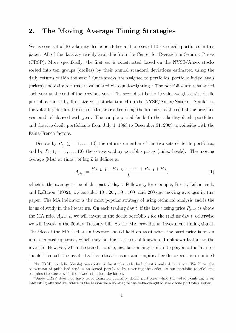
2. The Moving Average Timing Strategies
We use one set of 10 volatility decile portfolios and one set of 10 size decile portfolios in this
paper. All of the data are readily available from the Center for Research in Security Prices
(CRSP). More specifically, the first set is constructed based on the NYSE/Amex stocks
sorted into ten groups (deciles) by their annual standard deviations estimated using the
daily returns within the year.3 Once stocks are assigned to portfolios, portfolio index levels
(prices) and daily returns are calculated via equal-weighting.4 The portfolios are rebalanced
each year at the end of the previous year. The second set is the 10 value-weighted size decile
portfolios sorted by firm size with stocks traded on the NYSE/Amex/Nasdaq. Similar to
the volatility deciles, the size deciles are ranked using the firm size at the end of the previous
year and rebalanced each year. The sample period for both the volatility decile portfolios
and the size decile portfolios is from July 1, 1963 to December 31, 2009 to coincide with the
Fama-French factors.
Denote by Rjt (j = 1, . . . , 10) the returns on either of the two sets of decile portfolios,
and by Pjt (j = 1, . . . , 10) the corresponding portfolio prices (index levels). The moving
average (MA) at time t of lag L is defines as
Ajt,L =Pjt−L−1 + Pjt−L−2 + · · ·+ Pjt−1 + Pjt
L, (1)
which is the average price of the past L days. Following, for example, Brock, Lakonishok,
and LeBaron (1992), we consider 10-, 20-, 50-, 100- and 200-day moving averages in this
paper. The MA indicator is the most popular strategy of using technical analysis and is the
focus of study in the literature. On each trading day t, if the last closing price Pjt−1 is above
the MA price Ajt−1,L, we will invest in the decile portfolio j for the trading day t, otherwise
we will invest in the 30-day Treasury bill. So the MA provides an investment timing signal.
The idea of the MA is that an investor should hold an asset when the asset price is on an
uninterrupted up trend, which may be due to a host of known and unknown factors to the
investor. However, when the trend is broke, new factors may come into play and the investor
should then sell the asset. Its theoretical reasons and empirical evidence will be examined
3In CRSP, portfolio (decile) one contains the stocks with the highest standard deviation. We follow theconvention of published studies on sorted portfolios by reversing the order, so our portfolio (decile) onecontains the stocks with the lowest standard deviation.
4Since CRSP does not have value-weighted volatility decile portfolios while the value-weighting is aninteresting alternative, which is the reason we also analyze the value-weighted size decile portfolios below.
4
in the next section.
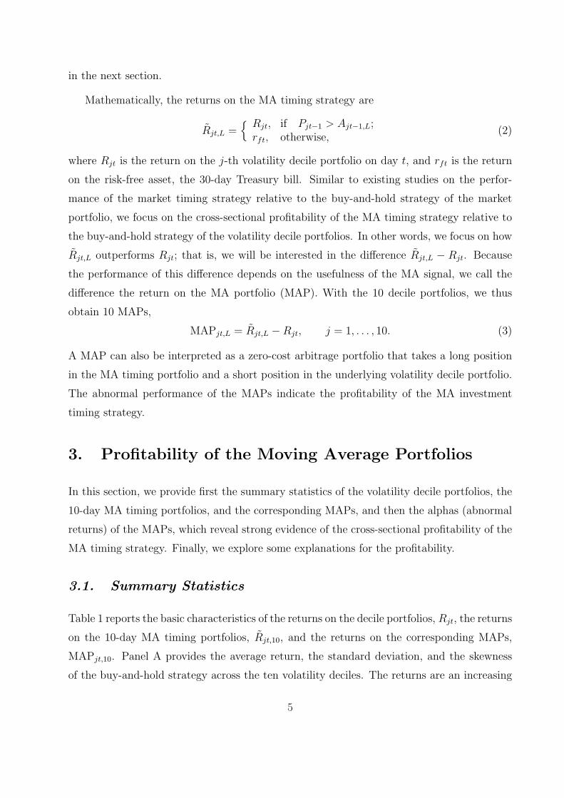
Mathematically, the returns on the MA timing strategy are
Rjt,L ={ Rjt, if Pjt−1 > Ajt−1,L;
rft, otherwise,(2)
where Rjt is the return on the j-th volatility decile portfolio on day t, and rft is the return
on the risk-free asset, the 30-day Treasury bill. Similar to existing studies on the perfor-
mance of the market timing strategy relative to the buy-and-hold strategy of the market
portfolio, we focus on the cross-sectional profitability of the MA timing strategy relative to
the buy-and-hold strategy of the volatility decile portfolios. In other words, we focus on how
Rjt,L outperforms Rjt; that is, we will be interested in the difference Rjt,L − Rjt. Because
the performance of this difference depends on the usefulness of the MA signal, we call the
difference the return on the MA portfolio (MAP). With the 10 decile portfolios, we thus
obtain 10 MAPs,
MAPjt,L = Rjt,L −Rjt, j = 1, . . . , 10. (3)
A MAP can also be interpreted as a zero-cost arbitrage portfolio that takes a long position
in the MA timing portfolio and a short position in the underlying volatility decile portfolio.
The abnormal performance of the MAPs indicate the profitability of the MA investment
timing strategy.
3. Profitability of the Moving Average Portfolios
In this section, we provide first the summary statistics of the volatility decile portfolios, the
10-day MA timing portfolios, and the corresponding MAPs, and then the alphas (abnormal
returns) of the MAPs, which reveal strong evidence of the cross-sectional profitability of the
MA timing strategy. Finally, we explore some explanations for the profitability.
3.1. Summary Statistics
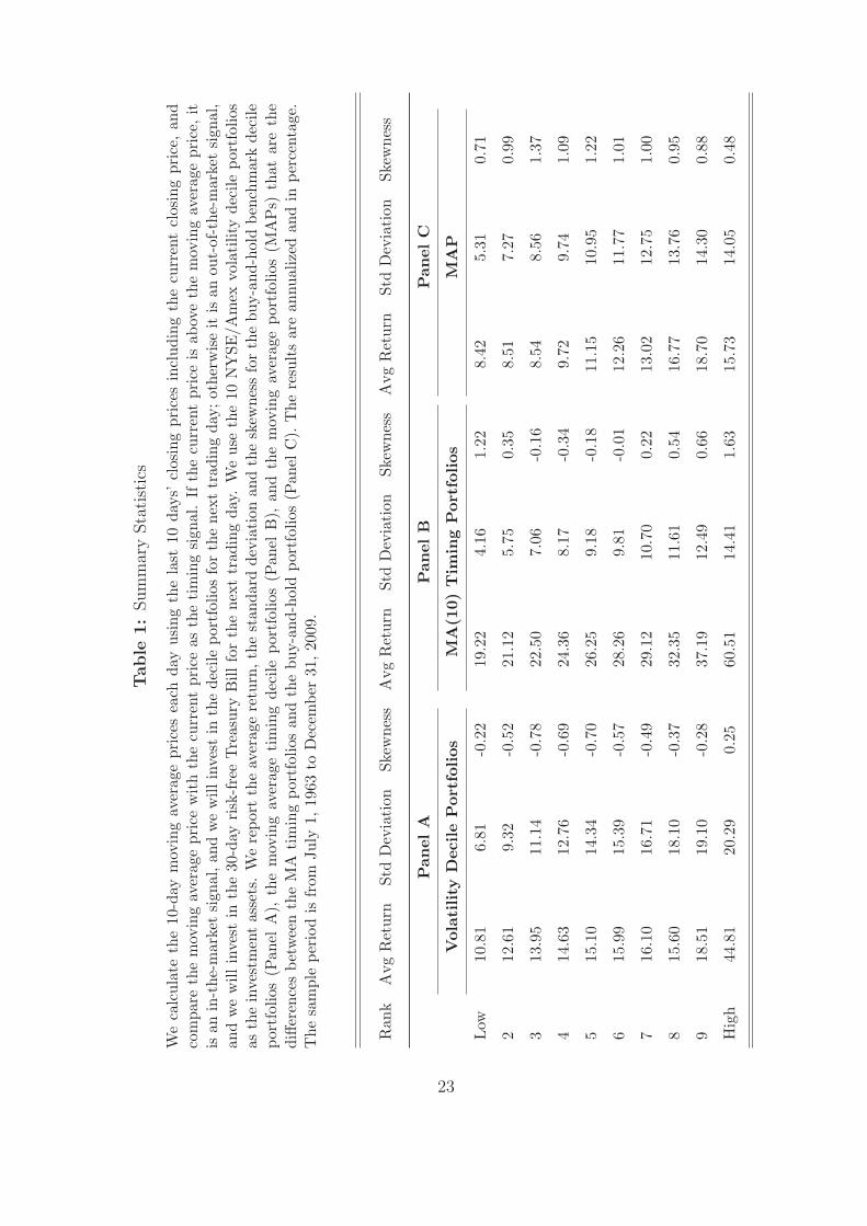
Table 1 reports the basic characteristics of the returns on the decile portfolios, Rjt, the returns
on the 10-day MA timing portfolios, Rjt,10, and the returns on the corresponding MAPs,
MAPjt,10. Panel A provides the average return, the standard deviation, and the skewness
of the buy-and-hold strategy across the ten volatility deciles. The returns are an increasing
5
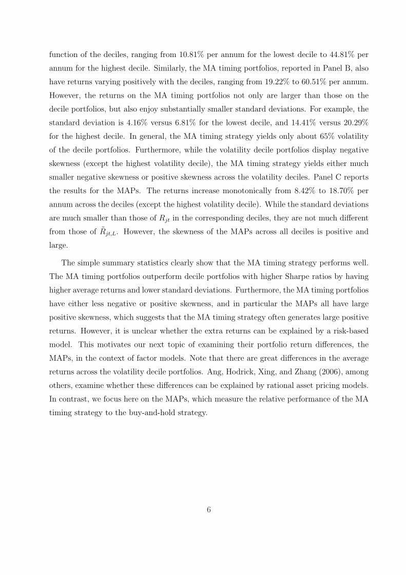
function of the deciles, ranging from 10.81% per annum for the lowest decile to 44.81% per
annum for the highest decile. Similarly, the MA timing portfolios, reported in Panel B, also
have returns varying positively with the deciles, ranging from 19.22% to 60.51% per annum.
However, the returns on the MA timing portfolios not only are larger than those on the
decile portfolios, but also enjoy substantially smaller standard deviations. For example, the
standard deviation is 4.16% versus 6.81% for the lowest decile, and 14.41% versus 20.29%
for the highest decile. In general, the MA timing strategy yields only about 65% volatility
of the decile portfolios. Furthermore, while the volatility decile portfolios display negative
skewness (except the highest volatility decile), the MA timing strategy yields either much
smaller negative skewness or positive skewness across the volatility deciles. Panel C reports
the results for the MAPs. The returns increase monotonically from 8.42% to 18.70% per
annum across the deciles (except the highest volatility decile). While the standard deviations
are much smaller than those of Rjt in the corresponding deciles, they are not much different
from those of Rjt,L. However, the skewness of the MAPs across all deciles is positive and
large.
The simple summary statistics clearly show that the MA timing strategy performs well.
The MA timing portfolios outperform decile portfolios with higher Sharpe ratios by having
higher average returns and lower standard deviations. Furthermore, the MA timing portfolios
have either less negative or positive skewness, and in particular the MAPs all have large
positive skewness, which suggests that the MA timing strategy often generates large positive
returns. However, it is unclear whether the extra returns can be explained by a risk-based
model. This motivates our next topic of examining their portfolio return differences, the
MAPs, in the context of factor models. Note that there are great differences in the average
returns across the volatility decile portfolios. Ang, Hodrick, Xing, and Zhang (2006), among
others, examine whether these differences can be explained by rational asset pricing models.
In contrast, we focus here on the MAPs, which measure the relative performance of the MA
timing strategy to the buy-and-hold strategy.
6
3.2. Alpha
Consider first the capital asset pricing model (CAPM) regression of the zero-cost portfolio
returns on the market portfolio,
MAPjt,L = αj + βj,mkt(Rmkt,t − rft) + εjt, j = 1, . . . , 10, (4)
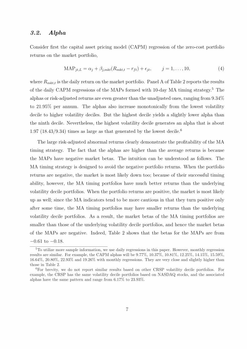
where Rmkt,t is the daily return on the market portfolio. Panel A of Table 2 reports the results
of the daily CAPM regressions of the MAPs formed with 10-day MA timing strategy.5 The
alphas or risk-adjusted returns are even greater than the unadjusted ones, ranging from 9.34%
to 21.95% per annum. The alphas also increase monotonically from the lowest volatility
decile to higher volatility deciles. But the highest decile yields a slightly lower alpha than
the ninth decile. Nevertheless, the highest volatility decile generates an alpha that is about
1.97 (18.43/9.34) times as large as that generated by the lowest decile.6
The large risk-adjusted abnormal returns clearly demonstrate the profitability of the MA
timing strategy. The fact that the alphas are higher than the average returns is because
the MAPs have negative market betas. The intuition can be understood as follows. The
MA timing strategy is designed to avoid the negative portfolio returns. When the portfolio
returns are negative, the market is most likely down too; because of their successful timing
ability, however, the MA timing portfolios have much better returns than the underlying
volatility decile portfolios. When the portfolio returns are positive, the market is most likely
up as well; since the MA indicators tend to be more cautious in that they turn positive only
after some time, the MA timing portfolios may have smaller returns than the underlying
volatility decile portfolios. As a result, the market betas of the MA timing portfolios are
smaller than those of the underlying volatility decile portfolios, and hence the market betas
of the MAPs are negative. Indeed, Table 2 shows that the betas for the MAPs are from
−0.61 to −0.18.
5To utilize more sample information, we use daily regressions in this paper. However, monthly regressionresults are similar. For example, the CAPM alphas will be 9.77%, 10.37%, 10.81%, 12.25%, 14.15%, 15.59%,16.64%, 20.80%, 22.93% and 19.26% with monthly regressions. They are very close and slightly higher thanthose in Table 2.
6For brevity, we do not report similar results based on other CRSP volatility decile portfolios. Forexample, the CRSP has the same volatility decile portfolios based on NASDAQ stocks, and the associatedalphas have the same pattern and range from 6.17% to 23.93%.
7
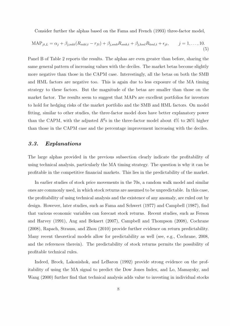
Consider further the alphas based on the Fama and French (1993) three-factor model,
MAPjt,L = αj + βj,mkt(Rmkt,t − rft) + βj,smbRsmb,t + βj,hmlRhml,t + εjt, j = 1, . . . , 10.(5)
Panel B of Table 2 reports the results. The alphas are even greater than before, sharing the
same general pattern of increasing values with the deciles. The market betas become slightly
more negative than those in the CAPM case. Interestingly, all the betas on both the SMB
and HML factors are negative too. This is again due to less exposure of the MA timing
strategy to these factors. But the magnitude of the betas are smaller than those on the
market factor. The results seem to suggest that MAPs are excellent portfolios for investors
to hold for hedging risks of the market portfolio and the SMB and HML factors. On model
fitting, similar to other studies, the three-factor model does have better explanatory power
than the CAPM, with the adjusted R2s in the three-factor model about 4% to 26% higher
than those in the CAPM case and the percentage improvement increasing with the deciles.
3.3. Explanations
The large alphas provided in the previous subsection clearly indicate the profitability of
using technical analysis, particularly the MA timing strategy. The question is why it can be
profitable in the competitive financial markets. This lies in the predictability of the market.
In earlier studies of stock price movements in the 70s, a random walk model and similar
ones are commonly used, in which stock returns are assumed to be unpredictable. In this case,
the profitability of using technical analysis and the existence of any anomaly, are ruled out by
design. However, later studies, such as Fama and Schwert (1977) and Campbell (1987), find
that various economic variables can forecast stock returns. Recent studies, such as Ferson
and Harvey (1991), Ang and Bekaert (2007), Campbell and Thompson (2008), Cochrane
(2008), Rapach, Strauss, and Zhou (2010) provide further evidence on return predictability.
Many recent theoretical models allow for predictability as well (see, e.g., Cochrane, 2008,
and the references therein). The predictability of stock returns permits the possibility of
profitable technical rules.
Indeed, Brock, Lakonishok, and LeBaron (1992) provide strong evidence on the prof-
itability of using the MA signal to predict the Dow Jones Index, and Lo, Mamaysky, and
Wang (2000) further find that technical analysis adds value to investing in individual stocks
8
beyond the index. Neely, Rapach, Tu, and Zhou (2010) provide the most recent evidence
on the value of technical analysis in forecasting market risk premium. Covering over 24,000
stocks spanning 22 years, Wilcox and Crittenden (2009) continue to find profitability of
technical analysis. Across various asset classes, Faber (2007) shows that technical analysis
improves the risk-adjusted returns. In other markets, such as the foreign exchange markets,
evidence on the profitability of technical analysis is even stronger. For example, LeBaron
(1999) and Neely (2002), among others, show that there are substantial gains with the use of
the MA signal and the gains are much larger than those for stock indices. Moreover, Gehrig
and Menkhoff (2006) argue that technical analysis is as important as fundamental analysis
to currency traders.
From a theoretical point of view, incomplete information on the fundamentals is a key for
investors to use technical analysis. In such a case, for example, Brown and Jennings (1989)
show that rational investors can gain from forming expectations based on historical prices,
and Blume, Easley, and O’Hara (1994) show that traders who use information contained
in market statistics do better than traders who do not. With incomplete information, the
investors can face model uncertainty even if the stock returns are predictable. In this case,
Zhu and Zhou (2009) show that MA strategies can help to learn about the predictability and
thus can add value to asset allocation. Note that both the MA and momentum strategies are
trend-following. The longer a trend continues, the more profitable the strategies may become.
Hence, models that explain momentum profits can also help to understand the profitability of
the MA indicators. In the market under-reaction theory, for example, Barberis, Shleifer, and
Vishny (1998) argue that prices can trend slowly when investors underweight new information
in making decisions. Daniel, Hirshleifer, and Subrahmanyam (1998) and Hong and Stein
(1999) show that behavior biases can also lead to price continuation. Moreover, Zhang
(2006) argues that stock price continuation is due to under-reaction to public information
by investors.
Explanations above help to understand why the MA strategy is profitable; the question
remains whether such profitability can be explained by compensation for risk. While this may
well be the case, the alphas we find for the MA strategies are large. Similar to the momentum
returns (see, e.g., Schwert, 2003; Jegadeesh and Titman, 1993, 2001), such magnitude of
abnormal returns is unlikely explained away by a more sophisticated and known asset pricing
model. Hence, we leave the search for new models in explaining the MAP anomaly to future
9
research.
4. Robustness
In this section, we examine the robustness of the profitability of the MAPs in several dimen-
sions. We first consider alternative lag lengths for the MA indicator, and then consider the
use of the value-weighted size decile portfolios. We analyze further the profitability of the
MA timing strategy when transaction costs are imposed. Finally we examine the profitability
in two subperiods.
4.1. Alternative Lag Lengths
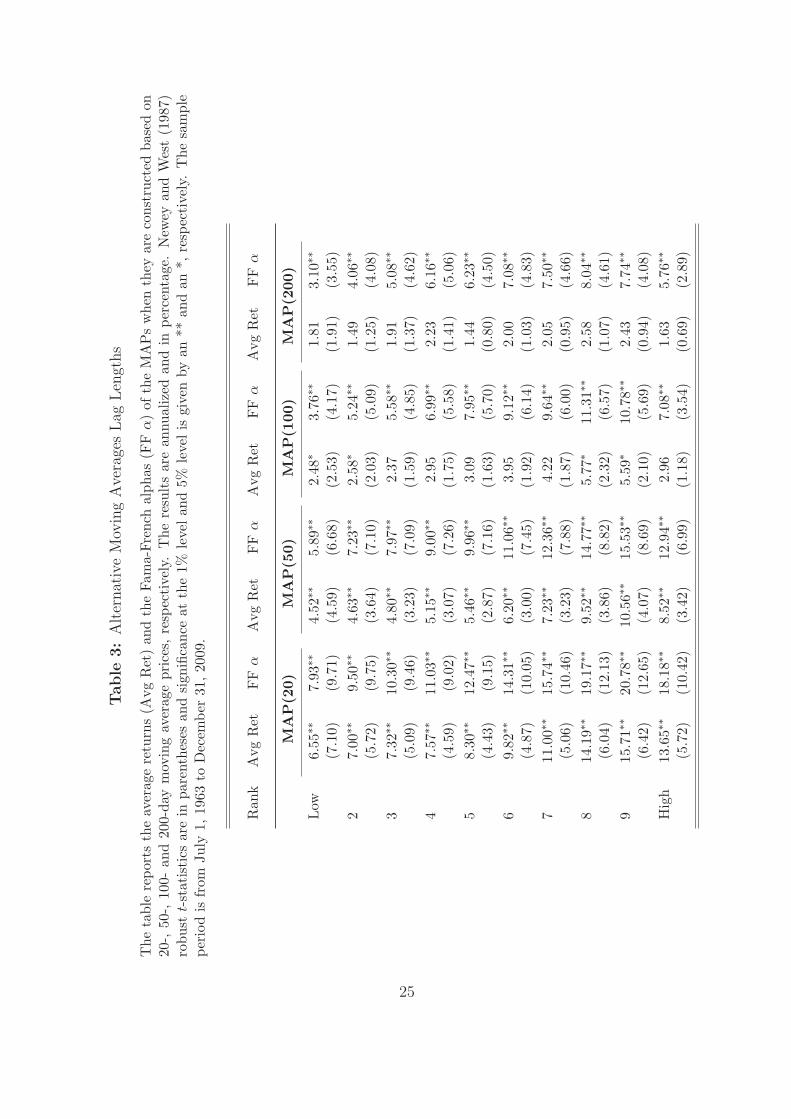
Consider now the profitability of the MAPs by using 20-day, 50-day, 100-day, and 200-day
moving averages. Table 3 reports both the average returns and Fama-French alphas for the
MAPs of the various lag lengths. The results are fundamentally the same as before, but two
interesting features emerge. First, the MA timing strategy still generates highly significant
abnormal returns relative to the buy-and-hold strategy regardless of the lag length used to
calculate the moving average price. This is reflected by the significantly positive returns and
significantly positive alphas of the MAPs. For example, even when the timing strategy is
based on the 200-day MA, the risk-adjusted abnormal returns range from 3.10% to 8.04%
per annum and are all significant. However, the magnitude of the abnormal returns does
decrease as the lag length increases. The decline is more apparent for the higher ranked
volatility decile portfolios, and accelerates after L = 20. For example, consider the case
for the highest decile portfolio. The Fama-French alpha with the 20-day MA is 18.18%
per annum, which is about 90% of the 10-day MA alpha (20.29% per annum reported in
Table 2). In contrast, the 50-day MA timing strategy generates a risk-adjusted abnormal
return of 12.94%, which is about 64% of the 10-day MA alpha. In addition, the 200-day MA
timing strategy only generates 5.76%, only about 29% of the risk-adjusted abnormal return
of the 10-day MA.
Second, similar to the 10-day MA timing strategy, all the other MA timing strategies
generate monotonically increasing abnormal returns across the deciles, except the highest
decile case where it has slightly lower values than those of the ninth decile. However, differ-
10

ences in the abnormal returns between the highest and lowest deciles decline as the lag length
increases. For example, the abnormal return of the highest decile is about 2.29 (18.18/7.93)
times of that of the lowest decile when L = 20, and only about 1.84 (5.71/3.09) times of
that of the lowest decile when L = 200.
4.2. Size Decile Portfolios
CRSP volatility decile portfolios are equal-weighted, which raises a concern about the larger
role the small stocks play in these portfolios than they play in the value-weighted case. To
mitigate this concern, we use the value-weighted size portfolios to further check the robust-
ness of the results. Since smaller size deciles have larger volatilities, the 10 size portfolios
may be viewed approximately as another set of volatility decile portfolios.
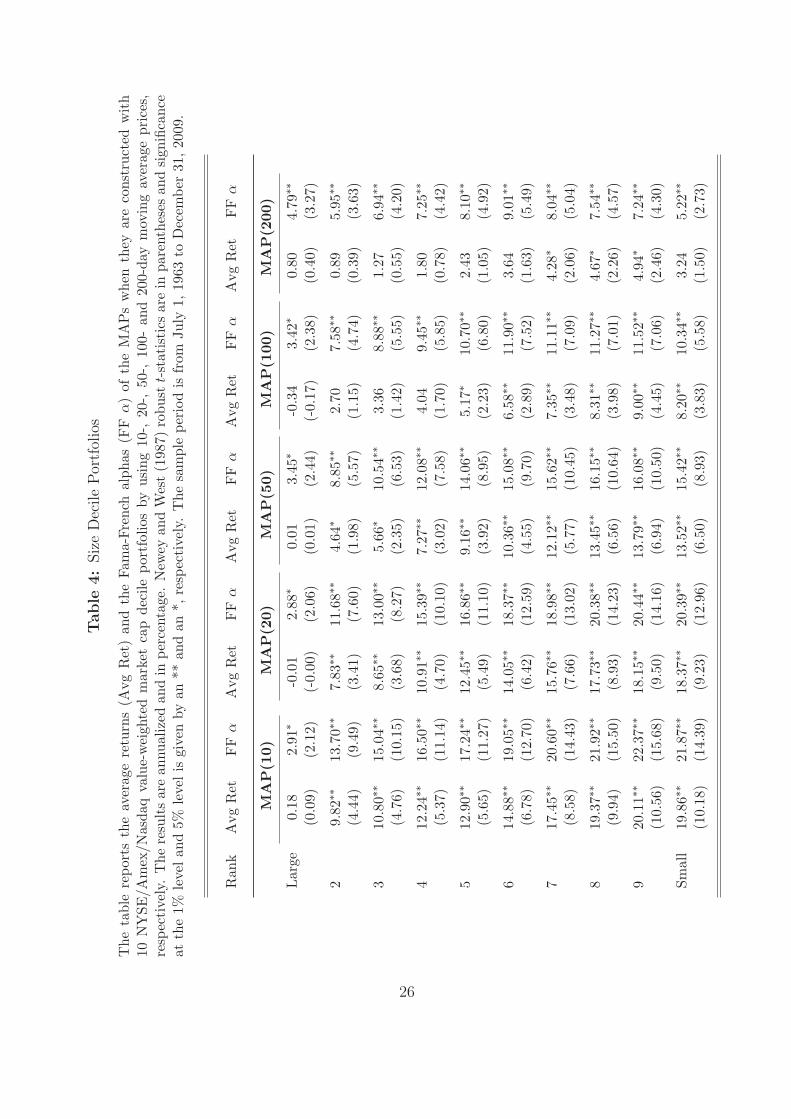
Table 4 reports the average returns and Fama-French alphas for the MAPs based on the
size portfolios formed with value-weighting based on stocks traded on NYSE/Amex/Nasdaq.7
With the important exception on the largest size portfolio which tends to have the least
volatile stocks, the results are similar to the previous ones using the volatility decile portfolios.
Across all the lag lengths, the alphas on the MAPs based on the largest size portfolio are
about only 3% per annum. Nevertheless, starting from the next largest decile (the 2nd decile),
both the average returns and Fama-French alphas increase from large stock deciles to small
stock deciles, and the magnitude is comparable to that of the volatility decile portfolios. For
example, the Fama-French alphas range from 13.70% to 22.37% when L = 10 and when the
largest size portfolio case is ignored. Overall, it is clear that the profitability of the MA
timing strategy remains strong with the use of the value-weighted size decile portfolios.
Small size effect was first documented by Banz (1981) and Reinganum (1981) who show
that small stocks traded on NYSE earn higher average returns than is predicted by the
CAPM. Many subsequent studies confirm the small size effect. Fama and French (1993) use
the small size effect to form the SMB factor. However, Schwert (2003) show that the small
size effect has disappeared after its initial publication.
Table 5 reports the results of the CAPM regressions of the size decile portfolios, and the
corresponding MAPs in the period from January 02, 2004 to December 31, 2009. All the
alphas of the size decile portfolios are insignificant in this subperiod, even for the smallest
7Similar results are obtained if the size decile portfolios are formed by using only NYSE stocks.
11
size decile, which is consistent with Schwert (2003). In contrast, the MAPs based on the
size portfolios still have significantly positive and alphas from decile seven to decile 10. In
addition, the abnormal returns are as large as before in magnitude, and are of great economic
significance. For example, the MAP for the smallest decile yield an annualized abnormal
return of 21.10%. It is interesting that while the size anomaly disappears in this subperiod,
the MA anomaly is alive and well. This suggests that trading the size portfolios can still
earn abnormal profits with the use of technical analysis.
4.3. Average Holding Days, Trading Frequency and TransactionCosts
Since the MA timing strategy is based on daily signals, it is of interest to see how often it
trades. If the trades occur too often, it will be of real concern whether the abnormal returns
can survive transaction costs. We address this issue by analyzing the average holding days
of the timing portfolios, their trading frequency, as well as their returns after accounting for
the trading costs.
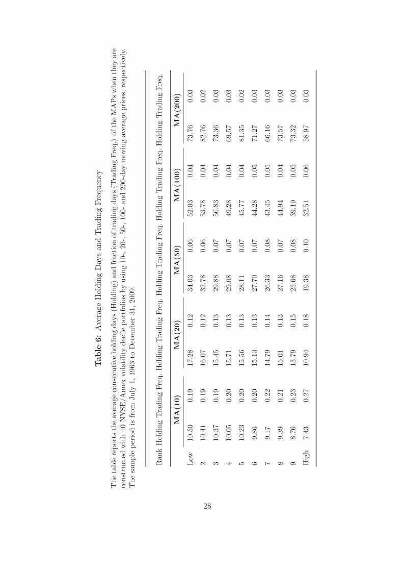
The average holding days are reported in Table 6. It is not surprising that longer lag
lengths result in longer average holding days as longer lag lengths capture longer trends.
For example, the 10-day MA timing strategy has about 9 to 10 holding days on average,
whereas the 200-day MA timing strategy has average holding days ranging from 59 to 83
days. In addition, the differences in the holding days across the deciles also increase with
the lag length. The lowest volatility deciles often has the longest holding days, whereas the
highest volatility decile often has the shortest holding days. To assess further on trading,
we also estimate the fraction of days when the trades occur relative to the total number of
days and report it as ‘Trading Frequency (Trade Freq.)’ in Table 6. Since longer lag lengths
have longer average holding days, the trading frequency is inversely related to the lag length.
For example, the 10-day MA strategy requires about 20% trading days, whereas the 200-day
MA has about only 3%, a very small number.
Consider now how the abnormal returns will be affected once we impose transaction
costs on all the trades. Intuitively, due to the large size of the abnormal returns, and due to
the modest amount of trading, the abnormal returns are likely to survive, especially for the
highest volatility decile portfolio. This is indeed the case as it turns out below.
12
Following Balduzzi and Lynch (1999), Lynch and Balduzzi (2000), and Han (2006), for
example, we assume that we incur transaction costs for trading the decile portfolios but no
costs for trading the 30-day Treasury Bill. Then, in the presence of transaction cost τ per
trade, the returns on the MA timing strategy are:
Rjt,L =
Rjt, if Pjt−1 > Ajt−1,L and Pjt−2 > Ajt−2,L;Rjt − τ, if Pjt−1 > Ajt−1,L and Pjt−2 < Ajt−2,L;rft, if Pjt−1 < Ajt−1,L and Pjt−2 < Ajt−2,L;rft − τ, if Pjt−1 < Ajt−1,L and Pjt−2 > Ajt−2,L.
(6)
Determining the appropriate transaction cost level is always a difficult issue, and recent
studies use a transaction cost level ranging from one basis point to 50 basis points. For
example, Balduzzi and Lynch (1999) use one basis point and 50 basis points as the lower and
upper bounds for transaction costs, and Lynch and Balduzzi (2000) consider a transaction
cost of 25 basis points. Following the latter, we set τ equal to 25 basis points, which amounts
to 63% (252× .25) per annum trading costs if one trades every trading day.
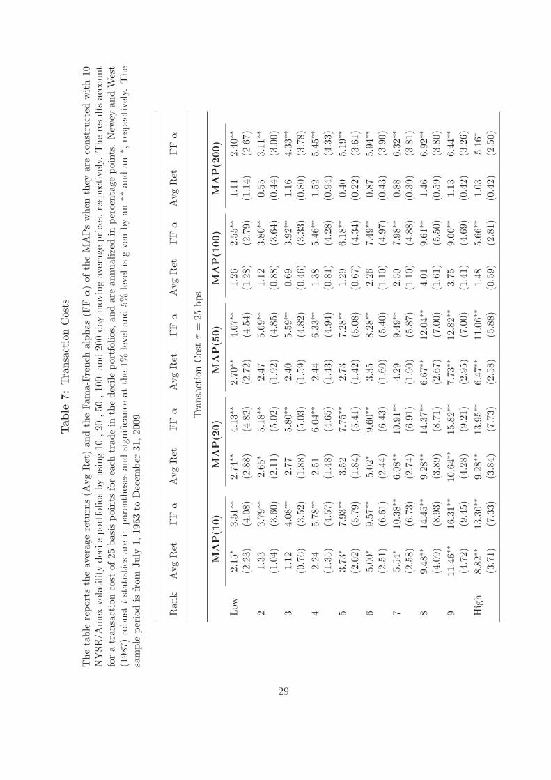
Table 7 reports the abnormal returns of the MAPs under the transaction cost of 25 basis
points per trade. The transaction cost has reduced the abnormal returns across the various
MA timing strategies. The 10-day MA strategy experiences the largest impact. Its abnor-
mal returns drop about 6 to 7% per annum on average due to its relatively high trading
frequency. However, the 20-day MA experiences only about 3 to 4% per annum drop in
abnormal performance, whereas the 200-day MA has only about 0.7 to 1.0% drop in the
abnormal returns. Nevertheless, all of the MAPs still have significantly positive abnormal
returns. Despite the presence of transaction costs, the 10-day MA timing strategy still gen-
erates greatly significant abnormal returns, 13.30% and 16.31% per annum, respectively, for
the highest decile and the ninth decile. Interestingly, though, after accounting for trans-
action costs, the 20-day MA timing strategy performs as strong as the 10-day MA timing
strategy. Overall, transaction costs have little impact on performance, and the MAPs still
have economically highly significant abnormal returns.
4.4. Subperiods
Now we further check the robustness of the profitability of the MA timing strategy by exam-
ining its performance over subperiods. To avoid possible bias in affecting the performance, we
simply divide the entire sample period into two subperiods with roughly equal time length.
13
Table 8 reports the abnormal returns and beta coefficients from both the CAPM and the
Fama-French models. In both subperiods, the MAPs yield significant and positive abnormal
returns, similar to the case of the entire sample period. Moreover, both the CAPM and
the Fama-French alphas increase monotonically across the deciles except for the highest
decile which often has lower alphas than the ninth decile. Once again, the market betas
are significantly negative, so are the SMB betas. In addition, the HML betas are largely
insignificant and small in the first subperiod, but are significant and negative in the second
subperiod.
However, both the CAPM and the Fama-French alphas are higher in the first subperiod
than in the second subperiod, and also higher than those from the entire sample period. For
example, the lowest volatility decile has a CAPM and Fama-French alpha of about 11.27%
and 12.72 % per annum, respectively, in the first subperiod, but the abnormal returns reduce
to 7.39% and 7.69% per annum, respectively, in the second subperiod, and are compared to
9.34% and 9.83% per annum, respectively, in the entire sample period. Overall, the results
continue to support that the MAPs, especially those high decile ones, constitute a new
anomaly in asset pricing.
5. Comparison with Momentum
In this section, we compare the MAPs with the momentum factor, both of which are trend-
following and zero-cost spread portfolios, by examining their performance over business cycles
and their sensitivities to default and liquidity risks.
5.1. Momentum Betas
With returns on the momentum factor (UMD) which is readily available from French’s web
site, we can compute the correlations between UMD and the MAPs, which range from -0.01
to 0.07 from the lowest volatility decile MAP to the highest volatility decile MAP.
Table 9 reports the regression results of the MAPs on the Fama-French three factors and
the momentum factor. Clearly, momentum does not explain the abnormal returns of the
MAPs. Similar to the CAPM model and Fama-French three-factor model, the alphas are
still significantly positive and monotonically increasing across the deciles except the highest
14
decile for which the alpha is reduced. Moreover, the four-factor alphas are even slightly larger
than those of the CAPM and Fama-French models. This is due to the negative exposure of
the MAPs on the momentum factor.
However, the momentum betas of the MAPs are statistically significant, which suggests
that there is some statistical relation between the MAPs and the UMD. This is not surprising
since both are trend-following strategies. However, the link is quite weak. The magnitude of
the momentum betas are very small, a reflection of the low correlations between the MAPs
and the momentum factor. Moreover, the additional explanatory power of the momentum
factor is quite small. The last column of Table 9 reports the differences of the four-factor
regression R2s with those of the earlier Fama-French three-factor regression (Table 2). The
incremental R2s are all less than 1%. Therefore, we conclude that the MAPs and the UMD
are substantially different trend-following strategies. The question is whether there is any
economic linkage between them, which we address below.
5.2. Business Cycles
Chordia and Shivakumar (2002) provide evidence that the profitability of momentum strate-
gies is related to business cycles. They show that momentum payoffs are reliably positive and
significant over expansionary periods, whereas they become negative and insignificant over
recessionary periods. However, Griffin, Ji, and Martin (2003) find that momentum is still
profitable over negative GDP growth periods and explain that the earlier finding of Chordia
and Shivakumar (2002) may be due to not skipping a month between ranking and invest-
ment periods and the NBER classification of economic states. Using a new hand-collected
data set of the London Stock Exchange from the Victorian era (1866–1907), thus obviating
any data mining concern, Chabot, Ghysels, and Jagannathan (2010) do not find a link be-
tween momentum profits and GDP growth, either. Therefore, the overall evidence that the
profitability of the momentum strategy is affected by the business cycles seems mixed. On
the other hand, Cooper, Gutierrez, and Hameed (2004) argue that the momentum strategy
is profitable only after an up market, where the up market is defined as having positive
returns in the past one, two, or three years. Huang (2006) finds similar evidence in the
international markets, and Chabot, Ghysels, and Jagannathan (2010) extend the results to
the early periods of the Victorian era.
15

In our comparison of the performance of both the UMD and the MAPs, we regress both
the UMD factor and MAPs, respectively, on the Fama-French three factors and either a Re-
cession dummy variable indicating the NBER specified recessionary periods, or an Up Market
dummy variable indicating the periods when the market return of the previous year is posi-
tive. Table 10 reports the results. Consistent with Griffin, Ji, and Martin (2003) and Chabot,
Ghysels, and Jagannathan (2010), the Recession dummy variable (Panel A) is negative but
insignificant for the UMD factor, suggesting that the momentum strategy is profitable in
both expansionary and recessionary periods, but the profits may be smaller in recessions. In
contrast, all the MAPs have significant coefficients for the Recession dummy. Furthermore,
the coefficients are all positive, indicating that the MA timing strategy generates higher ab-
normal profits in recessionary periods than in expansionary periods. Nevertheless, the MAPs
yield both economically and statistically significant risk-adjusted abnormal returns (alphas)
in both periods, with positive alphas ranging from 8.05% to 20.72% per annum in expansion-
ary periods and ranging from 18.75% to 37.91% per annum in recessionary periods. Because
of the exceptionally high abnormal returns generated by the MAPs during recessions, one
may suspect that the overall performance of the MAPs should be much higher than that in
the expansion periods. Table 2 clearly states that this is not the case. The reason is that
there are only a few recessionary periods over the entire sample period. Overall, we find that
the MAPs are more sensitive to recessions and more profitable in recessions than the UMD.
From an asset pricing perspective, this is valuable. In the case of negative returns on the
market (shortage of an asset), the positive returns are worth more than usual (the price of
the asset will be higher than normal).
Panel B of Table 10 reports the results with the Up Market dummy variable. Consis-
tent with Cooper, Gutierrez, and Hameed (2004), Huang (2006), and Chabot, Ghysels, and
Jagannathan (2010), the alpha of the UMD factor is insignificant, indicating that the mo-
mentum strategy has insignificant risk-adjusted abnormal returns following the down market,
whereas the coefficient of the Up Market dummy is statistically significant and economically
considerable, about 10.86% per annum. In contrast, the coefficients of the Up Market dummy
are negative for all the MAPs, and less than half of them are statistically significant. This is
probably due to mean-reversion in the price that cannot be immediately captured by the MA
timing strategy. Nevertheless, the abnormal returns of the MAPs are still highly significant
and positive following the up market. On the other hand, the abnormal returns of the MAPs
16
are much higher following the down market, a result that is very different from that of the
momentum factor, but similar to that of MAPs using the NBER recession dummy variable
in Panel A.
5.3. Default Risk
Chordia and Shivakumar (2002) provide evidence that momentum profits can be explained
by exposure to macroeconomic variables including default spread, defined as the yield spread
between BAA and AAA corporate bonds. They show that when regressing the momentum
returns on a number of macroeconomic variables, default spread has a negative and significant
coefficient. Avramov and Chordia (2006) also show that momentum profits are related to
the default spread. Avramov, Chordia, Jostova, and Philipov (2007) further argue that there
is a strong link between momentum and credit rating, and that the momentum profits are
exclusively generated by low-grade firms and are nonexistent among high-grade firms. Their
results suggest a positive relation between momentum profits and default spread.
Panel A of Table 11 reports the results of regressing the UMD factor and the MAPs on the
Fama-French three factors and the default spread separately. Consistent with Chordia and
Shivakumar (2002), the coefficient of the UMD factor on the default spread is negative and
significant. In contrast, the MAPs are insensitive to the default spread: all the coefficients
are positive but insignificant. Hence, on an economic ground as measured by the default
risk, the UMD and MAPs represent different risk exposures as well.
5.4. Liquidity Risk
Pastor and Stambaugh (2003) propose an aggregate liquidity measure and show that the
spread portfolio which takes a long position on the highest quintile portfolio and a short
position on the lowest quintile portfolio sorted on the aggregate liquidity can explain a certain
portion of the abnormal return from the UMD factor. However, Pastor and Stambaugh
(2003) also point out that the liquidity beta of the UMD factor is positive but insignificant.
Sadka (2006) also shows that momentum profits are related to liquidity risk premium.
Panel B of Table 11 reports the results of regressing separately both the UMD factor
and MAP portfolios on the Fama-French three factors and the aggregate liquidity measure
of Pastor and Stambaugh (2003). The momentum strategy has a negatively small beta and
17
is statistically insensitive to this aggregate liquidity measure, consistent with Pastor and
Stambaugh (2003). On the other hand, the coefficients of the MAPs are about twice or more
as negative. In addition, the R2s of the regressions are about 10 times as large as that of the
UMD. Once again, from the liquidity point of view, the UMD and MAPs are different too.
6. Concluding Remarks
In this paper, we document that a standard moving average of technical analysis, when
applied to portfolios sorted by volatility, can generate investment timing portfolios that
outperform the buy-and-hold strategy greatly, with returns that have negative or little risk
exposures on the market factor and the Fama-French SMB and HML factors. Especially
for the high volatility portfolios, the abnormal returns, relative to the CAPM and the Fama
and French (1993) three-factor models, are high, and higher than those from the momentum
strategy. The abnormal returns remain high even after accounting for transaction costs.
While the moving average strategy is a trend-following one similar to the momentum strategy,
its performance has little correlation with the momentum strategy, and behaves differently
over business cycles, and with respect to default and liquidity risks.
Our research provides new research avenues in several areas. First, our study suggests
that it will be likely fruitful to examine the profitability of technical analysis in various
markets and asset classes by investigating the cross-sectional performance, especially focusing
on portfolios sorted by volatility. Given the vast literature on technical analysis, potentially
many open questions may be explored and answered. Second, our study presents an exciting
new anomaly in the finance literature. Given the size of the abnormal returns and the wide
use of technical analysis, explaining the moving average anomaly with new asset pricing
models will be important and desirable. Thirdly, because of its trend-following nature,
various investment issues that have been investigated around the momentum strategies can
also be investigated for the moving average anomaly. All of these are interesting topics for
future research.
18
References
Ang, A., G. Bekaert, 2007. Stock return predictability: Is it there? The Review of Financial
Studies 20, 651–707.
Ang, A., R. J. Hodrick, Y. Xing, X. Zhang, 2006. The cross-section of volatility and expected
returns. Journal of Finance 61(1), 259–299.
Avramov, D., T. Chordia, 2006. Asset pricing models and financial market anomalies. The
Review of Financial Studies 19(3), 1001–1040.
Avramov, D., T. Chordia, G. Jostova, A. Philipov, 2007. Momentum and credit rating.
Journal of Finance 62(5), 2503–2520.
Balduzzi, P., A. W. Lynch, 1999. Transaction costs and predictability: Some utility cost
calculations. Journal of Financial Economics 52, 47–78.
Banz, R., 1981. The relationship between return and market value of common stock. Journal
of Financial Economics 9, 3–18.
Barberis, N., A. Shleifer, R. Vishny, 1998. A model of investor sentiment. Journal of Financial
Economics 49(3), 307–343.
Blume, L., D. Easley, M. O’Hara, 1994. Market statistics and technical analysis: The role of
volume. Journal of Finance 49(1), 153–81.
Brock, W., J. Lakonishok, B. LeBaron, 1992. Simple technical trading rules and the stochas-
tic properties of stock returns. The Journal of Finance 47(5), 1731–1764.
Brown, D. P., R. H. Jennings, 1989. On technical analysis. The Review of Financial Studies
2(4), 527–551.
Campbell, J. Y., 1987. Stock returns and the term structure. Journal of Financial Economics
18, 373–399.
Campbell, J. Y., S. B. Thompson, 2008. Predicting excess stock returns out of sample: Can
anything beat the historical average? The Review of Financial Studies 21(4), 1509–1532.
19
Chabot, B. R., E. Ghysels, R. Jagannathan, 2010. Momentum cycles and limits to arbitrage
- evidence from Victorian England and post-depression US stock markets. Unpublished
working paper.
Chordia, T., L. Shivakumar, 2002. Momentum, business cycle, and time-varying expected
returns. Journal of Finance 57(2), 985–1019.
Cochrane, J. H., 2008. The dog that did not bark: A defense of return predictability. Review
of Financial Studies 21(4), 1533–1575.
Cooper, M. J., R. C. Gutierrez, Jr., A. Hameed, 2004. Market states and momentum. The
Journal of Finance 59(3), 1345–1365.
Covel, M. W., 2005. Trend Following: How Great Traders Make Millions in Up or Down
Markets. Prentice-Hall, New York, New York.
Cowles, A., 1933. Can stock market forecasters forecast? Econometrica 1, 309–324.
Daniel, K., D. Hirshleifer, A. Subrahmanyam, 1998. Investor psychology and security market
under- and overreactions. Journal of Finance 53(6), 1839–1885.
Faber, M. T., 2007. A quantitative approach to tactical asset allocation. The Journal of
Wealth Management 9(4), 69–79.
Fama, E. F., K. R. French, 1993. Common risk factors in the returns on stocks and bonds.
Journal of Financial Economics 33, 3–56.
Fama, E. F., W. Schwert, 1977. Asset returns and inflation. Journal of Financial Economics
5, 115–146.
Ferson, W. E., C. R. Harvey, 1991. The variation of economic risk premiums. Journal of
Political Economy 99, 385–415.
Gehrig, T., L. Menkhoff, 2006. Extended evidence on the use of technical analysis in foreign
exchange. International Journal of Finance and Economics 11(4), 327–338.
Griffin, J. M., X. Ji, J. S. Martin, 2003. Momentum investing and business cycle risk: Evi-
dence from pole to pole. Journal of Finance 58, 2515–2547.
20
Han, Y., 2006. Asset allocation with a high dimensional latent factor stochastic volatility
model. The Review of Financial Studies 19(1), 237–271.
Han, Y., G. Zhou, 2010. The momentum anomaly: An enhanced strategy based on technical
analysis. Work in progress.
Hong, H., J. C. Stein, 1999. A unified theory of underreaction, momentum trading, and
overreaction in asset markets. Journal of Finance 54(6), 2143–2184.
Huang, D., 2006. Market states and international momentum strategies. The Quarterly Re-
view of Economics and Finance 46, 437–446.
Jegadeesh, N., S. Titman, 1993. Returns to buying winners and selling losers: Implications
for stock market efficiency. The Journal of Finance 48(1), 65–91.
, 2001. Profitability of momentum strategies: An evaluation of alternative explana-
tions. Journal of Finance 56(2), 699–720.
LeBaron, B., 1999. Technical trading rule profitability and foreign exchange intervention.
Journal of International Economics 49, 125–143.
Lo, A. W., J. Hasanhodzic, 2009. The Heretics of Finance: Conversations with Leading
Practitioners of Technical Analysis. Bloomberg Press, New York.
Lo, A. W., H. Mamaysky, J. Wang, 2000. Foundations of technical analysis: Computational
algorithms, statistical inference, and empirical implementation. The Journal of Finance
55(4), 1705–1770.
Lynch, A. W., P. Balduzzi, 2000. Predictability and transaction costs: The impact on rebal-
ancing rules and behavior. Journal of Finance 66(5), 2285–2309.
Neely, C. J., 2002. The temporal pattern of trading rule returns and central bank interven-
tion: intervention does not generate technical trading rule profits. Unpublished working
Papers, Federal Reserve Bank of St. Louis.
Neely, C. J., D. E. Rapach, J. Tu, G. Zhou, 2010. Out-of-sample equity premium prediction:
Fundamental vs. technical analysis. Unpublished working paper, Washington University
in St. Louis.
21
Newey, W. K., K. D. West, 1987. A simple, positive semi-definite, heteroskedasticity and
autocorrelation consistent covariance matrix. Econometrica 55, 703–708.
Pastor, L., R. Stambaugh, 2003. Liquidity risk and expected stock returns. Journal of Polit-
ical Economy 111(3), 642–685.
Rapach, D. E., J. K. Strauss, G. Zhou, 2010. Out-of-sample equity premium prediction:
Combination forecasts and links to the real economy. Review of Financial Studies 23(2),
821–862.
Reinganum, M. R., 1981. Misspecification of capital asset pricing: Empirical anomalies based
on earnings’ yields and market values. Journal of Financial Economics 9(1), 19–46.
Sadka, R., 2006. Momentum and post-earnings-announcement drift anomalies: The role of
liquidity risk. Journal of Financial Economics 80, 309–349.
Schwager, J. D., 1993. Market Wizards: Interviews with Top Traders. Collins, New York,
New York.
, 1995. The New Market Wizards: Conversations with America’s Top Traders. Wiley,
New York, New York.
Schwert, G. W., 2003. Anomalies and market efficiency. in Handbook of the Economics of
Finance, ed. by G. Constantinides, M. Harris, and R. M. Stulz. Elsevier Amsterdam,
Netherlands vol. 1 of Handbook of the Economics of Finance chap. 15, pp. 939–974.
Sullivan, R., A. Timmermann, H. White, 1999. Data snooping, technical trading rule per-
formance, and the bootstrap. Journal of Finance 54, 1647–1691.
Wilcox, C., E. Crittenden, 2009. Does trend following work on stocks? Unpublished working
paper.
Zhang, X. F., 2006. Information uncertainty and stock returns. Journal of Finance 61(1),
105–136.
Zhu, Y., G. Zhou, 2009. Technical analysis: An asset allocation perspective on the use of
moving averages. Journal of Financial Economics 92, 519–544.
22
Table
1:
Sum
mar
ySta
tist
ics
We
calc
ulat
eth
e10
-day
mov
ing
aver
age
pric
esea
chda
yus
ing
the
last
10da
ys’cl
osin
gpr
ices
incl
udin
gth
ecu
rren
tcl
osin
gpr
ice,
and
com
pare
the
mov
ing
aver
age
pric
ew
ith
the
curr
ent
pric
eas
the
tim
ing
sign
al.
Ifth
ecu
rren
tpr
ice
isab
ove
the
mov
ing
aver
age
pric
e,it
isan
in-t
he-m
arke
tsi
gnal
,and
we
will
inve
stin
the
deci
lepo
rtfo
lios
for
the
next
trad
ing
day;
othe
rwis
eit
isan
out-
of-t
he-m
arke
tsi
gnal
,an
dw
ew
illin
vest
inth
e30
-day
risk
-fre
eTre
asur
yB
illfo
rth
ene
xttr
adin
gda
y.W
eus
eth
e10
NY
SE/A
mex
vola
tilit
yde
cile
port
folio
sas
the
inve
stm
ent
asse
ts.
We
repo
rtth
eav
erag
ere
turn
,the
stan
dard
devi
atio
nan
dth
esk
ewne
ssfo
rth
ebu
y-an
d-ho
ldbe
nchm
ark
deci
lepo
rtfo
lios
(Pan
elA
),th
em
ovin
gav
erag
eti
min
gde
cile
port
folio
s(P
anel
B),
and
the
mov
ing
aver
age
port
folio
s(M
AP
s)th
atar
eth
edi
ffere
nces
betw
een
the
MA
tim
ing
port
folio
san
dth
ebu
y-an
d-ho
ldpo
rtfo
lios
(Pan
elC
).T
here
sult
sar
ean
nual
ized
and
inpe
rcen
tage
.T
hesa
mpl
epe
riod
isfr
omJu
ly1,
1963
toD
ecem
ber
31,20
09.
Ran
kA
vgR
etur
nSt
dD
evia
tion
Skew
ness
Avg
Ret
urn
Std
Dev
iati
onSk
ewne
ssA
vgR
etur
nSt
dD
evia
tion
Skew
ness
Pan
elA
Pan
elB
Pan
elC
Vol
atility
Dec
ile
Por
tfol
ios
MA
(10)
Tim
ing
Por
tfol
ios
MA
P
Low
10.8
16.
81-0
.22
19.2
24.
161.
228.
425.
310.
71
212
.61
9.32
-0.5
221
.12
5.75
0.35
8.51
7.27
0.99
313
.95
11.1
4-0
.78
22.5
07.
06-0
.16
8.54
8.56
1.37
414
.63
12.7
6-0
.69
24.3
68.
17-0
.34
9.72
9.74
1.09
515
.10
14.3
4-0
.70
26.2
59.
18-0
.18
11.1
510
.95
1.22
615
.99
15.3
9-0
.57
28.2
69.
81-0
.01
12.2
611
.77
1.01
716
.10
16.7
1-0
.49
29.1
210
.70
0.22
13.0
212
.75
1.00
815
.60
18.1
0-0
.37
32.3
511
.61
0.54
16.7
713
.76
0.95
918
.51
19.1
0-0
.28
37.1
912
.49
0.66
18.7
014
.30
0.88
Hig
h44
.81
20.2
90.
2560
.51
14.4
11.
6315
.73
14.0
50.
48
23
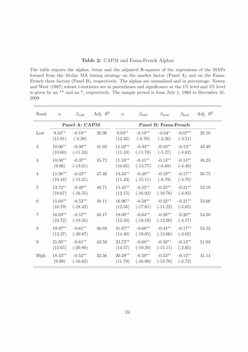
Table 2: CAPM and Fama-French Alphas
The table reports the alphas, betas and the adjusted R-squares of the regressions of the MAPsformed from the 10-day MA timing strategy on the market factor (Panel A) and on the Fama-French three factors (Panel B), respectively. The alphas are annualized and in percentage. Neweyand West (1987) robust t-statistics are in parentheses and significance at the 1% level and 5% levelis given by an ** and an *, respectively. The sample period is from July 1, 1963 to December 31,2009.
Rank α βmkt Adj. R2 α βmkt βsmb βhml Adj. R2
Panel A: CAPM Panel B: Fama-French
Low 9.34∗∗ -0.18∗∗ 26.96 9.83∗∗ -0.19∗∗ -0.04∗ -0.07∗∗ 28.10(11.81) (-8.20) (12.32) (-8.70) (-2.26) (-3.51)
2 10.06∗∗ -0.30∗∗ 41.02 11.02∗∗ -0.33∗∗ -0.10∗∗ -0.13∗∗ 43.49(10.60) (-11.33) (11.43) (-11.78) (-5.27) (-4.62)
3 10.50∗∗ -0.37∗∗ 45.72 11.58∗∗ -0.41∗∗ -0.13∗∗ -0.14∗∗ 48.23(9.86) (-13.61) (10.85) (-13.77) (-6.68) (-4.49)
4 11.98∗∗ -0.43∗∗ 47.40 13.34∗∗ -0.48∗∗ -0.19∗∗ -0.17∗∗ 50.75(10.18) (-15.21) (11.43) (-15.11) (-8.79) (-4.70)
5 13.72∗∗ -0.49∗∗ 48.71 15.45∗∗ -0.55∗∗ -0.25∗∗ -0.21∗∗ 53.19(10.67) (-16.55) (12.15) (-16.02) (-10.76) (-4.83)
6 15.04∗∗ -0.53∗∗ 48.11 16.96∗∗ -0.59∗∗ -0.32∗∗ -0.21∗∗ 53.68(10.79) (-18.42) (12.56) (-17.61) (-11.22) (-5.05)
7 16.03∗∗ -0.57∗∗ 48.17 18.00∗∗ -0.64∗∗ -0.38∗∗ -0.20∗∗ 54.20(10.72) (-19.35) (12.50) (-18.19) (-12.00) (-4.57)
8 19.97∗∗ -0.61∗∗ 46.93 21.87∗∗ -0.68∗∗ -0.44∗∗ -0.17∗∗ 53.52(12.37) (-20.87) (14.40) (-19.05) (-12.66) (-3.62)
9 21.95∗∗ -0.61∗∗ 43.59 23.72∗∗ -0.68∗∗ -0.50∗∗ -0.13∗∗ 51.03(12.65) (-20.80) (14.57) (-19.20) (-15.11) (-2.65)
High 18.43∗∗ -0.52∗∗ 32.56 20.29∗∗ -0.59∗∗ -0.53∗∗ -0.13∗∗ 41.14(9.99) (-16.62) (11.79) (-16.00) (-13.76) (-2.72)
24
Table
3:
Alt
ernat
ive
Mov
ing
Ave
rage
sLag
Len
gths
The
tabl
ere
port
sth
eav
erag
ere
turn
s(A
vgR
et)
and
the
Fam
a-Fr
ench
alph
as(F
Fα)
ofth
eM
AP
sw
hen
they
are
cons
truc
ted
base
don
20-,
50-,
100-
and
200-
day
mov
ing
aver
age
pric
es,re
spec
tive
ly.
The
resu
lts
are
annu
aliz
edan
din
perc
enta
ge.
New
eyan
dW
est
(198
7)ro
bust
t-st
atis
tics
are
inpa
rent
hese
san
dsi
gnifi
canc
eat
the
1%le
velan
d5%
leve
lis
give
nby
an**
and
an*,
resp
ecti
vely
.T
hesa
mpl
epe
riod
isfr
omJu
ly1,
1963
toD
ecem
ber
31,20
09.
Ran
kA
vgR
etFF
αA
vgR
etFF
αA
vgR
etFF
αA
vgR
etFF
α
MA
P(2
0)M
AP
(50)
MA
P(1
00)
MA
P(2
00)
Low
6.55∗∗
7.93∗∗
4.52∗∗
5.89∗∗
2.48∗
3.76∗∗
1.81
3.10∗∗
(7.1
0)(9
.71)
(4.5
9)(6
.68)
(2.5
3)(4
.17)
(1.9
1)(3
.55)
27.
00∗∗
9.50∗∗
4.63∗∗
7.23∗∗
2.58∗
5.24∗∗
1.49
4.06∗∗
(5.7
2)(9
.75)
(3.6
4)(7
.10)
(2.0
3)(5
.09)
(1.2
5)(4
.08)
37.
32∗∗
10.3
0∗∗
4.80∗∗
7.97∗∗
2.37
5.58∗∗
1.91
5.08∗∗
(5.0
9)(9
.46)
(3.2
3)(7
.09)
(1.5
9)(4
.85)
(1.3
7)(4
.62)
47.
57∗∗
11.0
3∗∗
5.15∗∗
9.00∗∗
2.95
6.99∗∗
2.23
6.16∗∗
(4.5
9)(9
.02)
(3.0
7)(7
.26)
(1.7
5)(5
.58)
(1.4
1)(5
.06)
58.
30∗∗
12.4
7∗∗
5.46∗∗
9.96∗∗
3.09
7.95∗∗
1.44
6.23∗∗
(4.4
3)(9
.15)
(2.8
7)(7
.16)
(1.6
3)(5
.70)
(0.8
0)(4
.50)
69.
82∗∗
14.3
1∗∗
6.20∗∗
11.0
6∗∗
3.95
9.12∗∗
2.00
7.08∗∗
(4.8
7)(1
0.05
)(3
.00)
(7.4
5)(1
.92)
(6.1
4)(1
.03)
(4.8
3)7
11.0
0∗∗
15.7
4∗∗
7.23∗∗
12.3
6∗∗
4.22
9.64∗∗
2.05
7.50∗∗
(5.0
6)(1
0.46
)(3
.23)
(7.8
8)(1
.87)
(6.0
0)(0
.95)
(4.6
6)8
14.1
9∗∗
19.1
7∗∗
9.52∗∗
14.7
7∗∗
5.77∗
11.3
1∗∗
2.58
8.04∗∗
(6.0
4)(1
2.13
)(3
.86)
(8.8
2)(2
.32)
(6.5
7)(1
.07)
(4.6
1)9
15.7
1∗∗
20.7
8∗∗
10.5
6∗∗
15.5
3∗∗
5.59∗
10.7
8∗∗
2.43
7.74∗∗
(6.4
2)(1
2.65
)(4
.07)
(8.6
9)(2
.10)
(5.6
9)(0
.94)
(4.0
8)H
igh
13.6
5∗∗
18.1
8∗∗
8.52∗∗
12.9
4∗∗
2.96
7.08∗∗
1.63
5.76∗∗
(5.7
2)(1
0.42
)(3
.42)
(6.9
9)(1
.18)
(3.5
4)(0
.69)
(2.8
9)
25
Table
4:
Siz
eD
ecile
Por
tfol
ios
The
tabl
ere
port
sth
eav
erag
ere
turn
s(A
vgR
et)
and
the
Fam
a-Fr
ench
alph
as(F
Fα)
ofth
eM
AP
sw
hen
they
are
cons
truc
ted
wit
h10
NY
SE/A
mex
/Nas
daq
valu
e-w
eigh
ted
mar
ket
cap
deci
lepo
rtfo
lios
byus
ing
10-,
20-,
50-,
100-
and
200-
day
mov
ing
aver
age
pric
es,
resp
ecti
vely
.T
here
sult
sar
ean
nual
ized
and
inpe
rcen
tage
.N
ewey
and
Wes
t(1
987)
robu
stt-
stat
isti
csar
ein
pare
nthe
ses
and
sign
ifica
nce
atth
e1%
leve
lan
d5%
leve
lis
give
nby
an**
and
an*,
resp
ecti
vely
.T
hesa
mpl
epe
riod
isfr
omJu
ly1,
1963
toD
ecem
ber
31,20
09.
Ran
kA
vgR
etFF
αA
vgR
etFF
αA
vgR
etFF
αA
vgR
etFF
αA
vgR
etFF
α
MA
P(1
0)M
AP
(20)
MA
P(5
0)M
AP
(100
)M
AP
(200
)
Lar
ge0.
182.
91∗
-0.0
12.
88∗
0.01
3.45∗
-0.3
43.
42∗
0.80
4.79∗∗
(0.0
9)(2
.12)
(-0.
00)
(2.0
6)(0
.01)
(2.4
4)(-
0.17
)(2
.38)
(0.4
0)(3
.27)
29.
82∗∗
13.7
0∗∗
7.83∗∗
11.6
8∗∗
4.64∗
8.85∗∗
2.70
7.58∗∗
0.89
5.95∗∗
(4.4
4)(9
.49)
(3.4
1)(7
.60)
(1.9
8)(5
.57)
(1.1
5)(4
.74)
(0.3
9)(3
.63)
310
.80∗∗
15.0
4∗∗
8.65∗∗
13.0
0∗∗
5.66∗
10.5
4∗∗
3.36
8.88∗∗
1.27
6.94∗∗
(4.7
6)(1
0.15
)(3
.68)
(8.2
7)(2
.35)
(6.5
3)(1
.42)
(5.5
5)(0
.55)
(4.2
0)
412
.24∗∗
16.5
0∗∗
10.9
1∗∗
15.3
9∗∗
7.27∗∗
12.0
8∗∗
4.04
9.45∗∗
1.80
7.25∗∗
(5.3
7)(1
1.14
)(4
.70)
(10.
10)
(3.0
2)(7
.58)
(1.7
0)(5
.85)
(0.7
8)(4
.42)
512
.90∗∗
17.2
4∗∗
12.4
5∗∗
16.8
6∗∗
9.16∗∗
14.0
6∗∗
5.17∗
10.7
0∗∗
2.43
8.10∗∗
(5.6
5)(1
1.27
)(5
.49)
(11.
10)
(3.9
2)(8
.95)
(2.2
3)(6
.80)
(1.0
5)(4
.92)
614
.88∗∗
19.0
5∗∗
14.0
5∗∗
18.3
7∗∗
10.3
6∗∗
15.0
8∗∗
6.58∗∗
11.9
0∗∗
3.64
9.01∗∗
(6.7
8)(1
2.70
)(6
.42)
(12.
59)
(4.5
5)(9
.70)
(2.8
9)(7
.52)
(1.6
3)(5
.49)
717
.45∗∗
20.6
0∗∗
15.7
6∗∗
18.9
8∗∗
12.1
2∗∗
15.6
2∗∗
7.35∗∗
11.1
1∗∗
4.28∗
8.04∗∗
(8.5
8)(1
4.43
)(7
.66)
(13.
02)
(5.7
7)(1
0.45
)(3
.48)
(7.0
9)(2
.06)
(5.0
4)
819
.37∗∗
21.9
2∗∗
17.7
3∗∗
20.3
8∗∗
13.4
5∗∗
16.1
5∗∗
8.31∗∗
11.2
7∗∗
4.67∗
7.54∗∗
(9.9
4)(1
5.50
)(8
.93)
(14.
23)
(6.5
6)(1
0.64
)(3
.98)
(7.0
1)(2
.26)
(4.5
7)
920
.11∗∗
22.3
7∗∗
18.1
5∗∗
20.4
4∗∗
13.7
9∗∗
16.0
8∗∗
9.00∗∗
11.5
2∗∗
4.94∗
7.24∗∗
(10.
56)
(15.
68)
(9.5
0)(1
4.16
)(6
.94)
(10.
50)
(4.4
5)(7
.06)
(2.4
6)(4
.30)
Smal
l19
.86∗∗
21.8
7∗∗
18.3
7∗∗
20.3
9∗∗
13.5
2∗∗
15.4
2∗∗
8.20∗∗
10.3
4∗∗
3.24
5.22∗∗
(10.
18)
(14.
39)
(9.2
3)(1
2.96
)(6
.50)
(8.9
3)(3
.83)
(5.5
8)(1
.50)
(2.7
3)
26
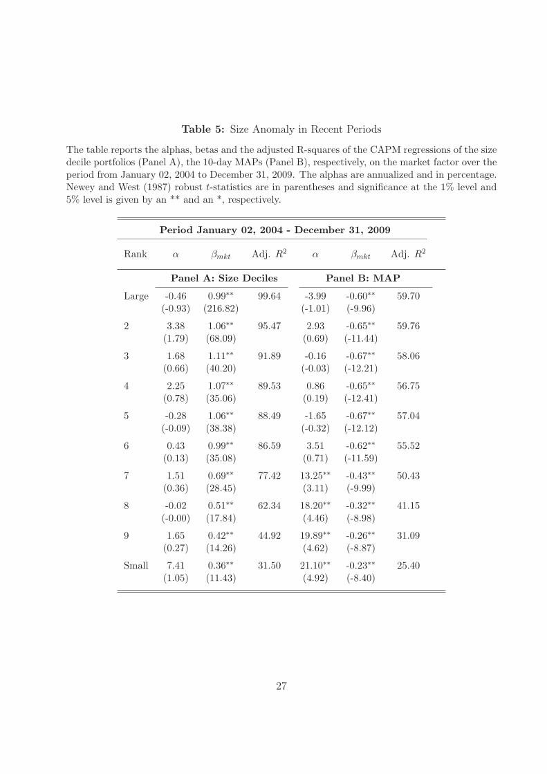
Table 5: Size Anomaly in Recent Periods
The table reports the alphas, betas and the adjusted R-squares of the CAPM regressions of the sizedecile portfolios (Panel A), the 10-day MAPs (Panel B), respectively, on the market factor over theperiod from January 02, 2004 to December 31, 2009. The alphas are annualized and in percentage.Newey and West (1987) robust t-statistics are in parentheses and significance at the 1% level and5% level is given by an ** and an *, respectively.
Period January 02, 2004 - December 31, 2009
Rank α βmkt Adj. R2 α βmkt Adj. R2
Panel A: Size Deciles Panel B: MAP
Large -0.46 0.99∗∗ 99.64 -3.99 -0.60∗∗ 59.70(-0.93) (216.82) (-1.01) (-9.96)
2 3.38 1.06∗∗ 95.47 2.93 -0.65∗∗ 59.76(1.79) (68.09) (0.69) (-11.44)
3 1.68 1.11∗∗ 91.89 -0.16 -0.67∗∗ 58.06(0.66) (40.20) (-0.03) (-12.21)
4 2.25 1.07∗∗ 89.53 0.86 -0.65∗∗ 56.75(0.78) (35.06) (0.19) (-12.41)
5 -0.28 1.06∗∗ 88.49 -1.65 -0.67∗∗ 57.04(-0.09) (38.38) (-0.32) (-12.12)
6 0.43 0.99∗∗ 86.59 3.51 -0.62∗∗ 55.52(0.13) (35.08) (0.71) (-11.59)
7 1.51 0.69∗∗ 77.42 13.25∗∗ -0.43∗∗ 50.43(0.36) (28.45) (3.11) (-9.99)
8 -0.02 0.51∗∗ 62.34 18.20∗∗ -0.32∗∗ 41.15(-0.00) (17.84) (4.46) (-8.98)
9 1.65 0.42∗∗ 44.92 19.89∗∗ -0.26∗∗ 31.09(0.27) (14.26) (4.62) (-8.87)
Small 7.41 0.36∗∗ 31.50 21.10∗∗ -0.23∗∗ 25.40(1.05) (11.43) (4.92) (-8.40)
27
Table
6:
Ave
rage
Hol
din
gD
ays
and
Tra
din
gFre
quen
cy
The
tabl
ere
port
sth
eav
erag
eco
nsec
utiv
eho
ldin
gda
ys(H
oldi
ng)an
dfr
acti
onof
trad
ing
days
(Tra
ding
Freq
.)of
the
MA
Psw
hen
they
are
cons
truc
ted
wit
h10
NY
SE/A
mex
vola
tilit
yde
cile
port
folio
sby
usin
g10
-,20
-,50
-,10
0-an
d20
0-da
ym
ovin
gav
erag
epr
ices
,res
pect
ivel
y.T
hesa
mpl
epe
riod
isfr
omJu
ly1,
1963
toD
ecem
ber
31,20
09.
Ran
kH
oldi
ngTra
ding
Freq
.H
oldi
ngTra
ding
Freq
.H
oldi
ngTra
ding
Freq
.H
oldi
ngTra
ding
Freq
.H
oldi
ngTra
ding
Freq
.
MA
(10)
MA
(20)
MA
(50)
MA
(100
)M
A(2
00)
Low
10.5
00.
1917
.28
0.12
34.0
30.
0652
.03
0.04
73.7
60.
03
210
.41
0.19
16.0
70.
1232
.78
0.06
53.7
80.
0482
.76
0.02
310
.37
0.19
15.4
50.
1329
.88
0.07
50.8
30.
0473
.36
0.03
410
.05
0.20
15.7
10.
1329
.08
0.07
49.2
80.
0469
.57
0.03
510
.23
0.20
15.5
60.
1328
.11
0.07
45.7
70.
0481
.35
0.02
69.
860.
2015
.13
0.13
27.7
00.
0744
.28
0.05
71.2
70.
03
79.
170.
2214
.79
0.14
26.3
30.
0843
.45
0.05
66.1
60.
03
89.
390.
2115
.01
0.13
27.1
60.
0744
.94
0.04
73.5
70.
03
98.
760.
2313
.79
0.15
25.6
80.
0839
.19
0.05
73.3
20.
03
Hig
h7.
430.
2710
.94
0.18
19.3
80.
1032
.51
0.06
58.9
70.
03
28
Table
7:
Tra
nsa
ctio
nC
osts
The
tabl
ere
port
sth
eav
erag
ere
turn
s(A
vgR
et)
and
the
Fam
a-Fr
ench
alph
as(F
Fα)
ofth
eM
AP
sw
hen
they
are
cons
truc
ted
wit
h10
NY
SE/A
mex
vola
tilit
yde
cile
port
folio
sby
usin
g10
-,20
-,50
-,10
0-an
d20
0-da
ym
ovin
gav
erag
epr
ices
,res
pect
ivel
y.T
here
sult
sac
coun
tfo
ra
tran
sact
ion
cost
of25
basi
spo
ints
for
each
trad
ein
the
deci
lepo
rtfo
lios,
and
are
annu
aliz
edin
perc
enta
gepo
ints
.N
ewey
and
Wes
t(1
987)
robu
stt-
stat
isti
csar
ein
pare
nthe
ses
and
sign
ifica
nce
atth
e1%
leve
lan
d5%
leve
lis
give
nby
an**
and
an*,
resp
ecti
vely
.T
hesa
mpl
epe
riod
isfr
omJu
ly1,
1963
toD
ecem
ber
31,20
09.
Ran
kA
vgR
etFF
αA
vgR
etFF
αA
vgR
etFF
αA
vgR
etFF
αA
vgR
etFF
α
Tra
nsac
tion
Cos
tτ
=25
bps
MA
P(1
0)M
AP
(20)
MA
P(5
0)M
AP
(100
)M
AP
(200
)
Low
2.15∗
3.51∗∗
2.74∗∗
4.13∗∗
2.70∗∗
4.07∗∗
1.26
2.55∗∗
1.11
2.40∗∗
(2.2
3)(4
.08)
(2.8
8)(4
.82)
(2.7
2)(4
.54)
(1.2
8)(2
.79)
(1.1
4)(2
.67)
21.
333.
79∗∗
2.65∗
5.18∗∗
2.47
5.09∗∗
1.12
3.80∗∗
0.55
3.11∗∗
(1.0
4)(3
.60)
(2.1
1)(5
.02)
(1.9
2)(4
.85)
(0.8
8)(3
.64)
(0.4
4)(3
.00)
31.
124.
08∗∗
2.77
5.80∗∗
2.40
5.59∗∗
0.69
3.92∗∗
1.16
4.33∗∗
(0.7
6)(3
.52)
(1.8
8)(5
.03)
(1.5
9)(4
.82)
(0.4
6)(3
.33)
(0.8
0)(3
.78)
42.
245.
78∗∗
2.51
6.04∗∗
2.44
6.33∗∗
1.38
5.46∗∗
1.52
5.45∗∗
(1.3
5)(4
.57)
(1.4
8)(4
.65)
(1.4
3)(4
.94)
(0.8
1)(4
.28)
(0.9
4)(4
.33)
53.
73∗
7.93∗∗
3.52
7.75∗∗
2.73
7.28∗∗
1.29
6.18∗∗
0.40
5.19∗∗
(2.0
2)(5
.79)
(1.8
4)(5
.41)
(1.4
2)(5
.08)
(0.6
7)(4
.34)
(0.2
2)(3
.61)
65.
00∗
9.57∗∗
5.02∗
9.60∗∗
3.35
8.28∗∗
2.26
7.49∗∗
0.87
5.94∗∗
(2.5
1)(6
.61)
(2.4
4)(6
.43)
(1.6
0)(5
.40)
(1.1
0)(4
.97)
(0.4
3)(3
.90)
75.
54∗
10.3
8∗∗
6.08∗∗
10.9
1∗∗
4.29
9.49∗∗
2.50
7.98∗∗
0.88
6.32∗∗
(2.5
8)(6
.73)
(2.7
4)(6
.91)
(1.9
0)(5
.87)
(1.1
0)(4
.88)
(0.3
9)(3
.81)
89.
48∗∗
14.4
5∗∗
9.28∗∗
14.3
7∗∗
6.67∗∗
12.0
4∗∗
4.01
9.61∗∗
1.46
6.92∗∗
(4.0
9)(8
.93)
(3.8
9)(8
.71)
(2.6
7)(7
.00)
(1.6
1)(5
.50)
(0.5
9)(3
.80)
911
.46∗∗
16.3
1∗∗
10.6
4∗∗
15.8
2∗∗
7.73∗∗
12.8
2∗∗
3.75
9.00∗∗
1.13
6.44∗∗
(4.7
2)(9
.45)
(4.2
8)(9
.21)
(2.9
5)(7
.00)
(1.4
1)(4
.69)
(0.4
2)(3
.26)
Hig
h8.
82∗∗
13.3
0∗∗
9.28∗∗
13.9
5∗∗
6.47∗∗
11.0
6∗∗
1.48
5.66∗∗
1.03
5.16∗
(3.7
1)(7
.33)
(3.8
4)(7
.73)
(2.5
8)(5
.88)
(0.5
9)(2
.81)
(0.4
2)(2
.50)
29
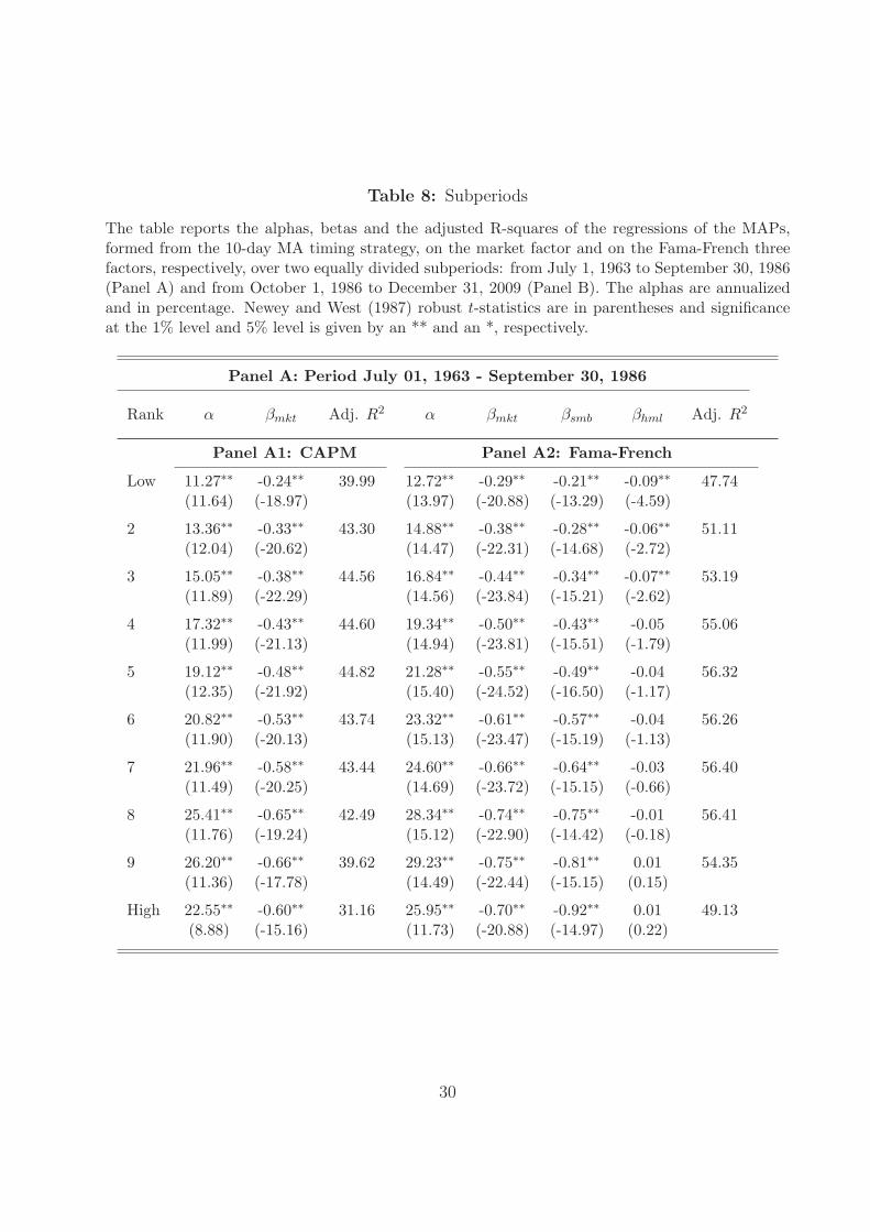
Table 8: Subperiods
The table reports the alphas, betas and the adjusted R-squares of the regressions of the MAPs,formed from the 10-day MA timing strategy, on the market factor and on the Fama-French threefactors, respectively, over two equally divided subperiods: from July 1, 1963 to September 30, 1986(Panel A) and from October 1, 1986 to December 31, 2009 (Panel B). The alphas are annualizedand in percentage. Newey and West (1987) robust t-statistics are in parentheses and significanceat the 1% level and 5% level is given by an ** and an *, respectively.
Panel A: Period July 01, 1963 - September 30, 1986
Rank α βmkt Adj. R2 α βmkt βsmb βhml Adj. R2
Panel A1: CAPM Panel A2: Fama-French
Low 11.27∗∗ -0.24∗∗ 39.99 12.72∗∗ -0.29∗∗ -0.21∗∗ -0.09∗∗ 47.74(11.64) (-18.97) (13.97) (-20.88) (-13.29) (-4.59)
2 13.36∗∗ -0.33∗∗ 43.30 14.88∗∗ -0.38∗∗ -0.28∗∗ -0.06∗∗ 51.11(12.04) (-20.62) (14.47) (-22.31) (-14.68) (-2.72)
3 15.05∗∗ -0.38∗∗ 44.56 16.84∗∗ -0.44∗∗ -0.34∗∗ -0.07∗∗ 53.19(11.89) (-22.29) (14.56) (-23.84) (-15.21) (-2.62)
4 17.32∗∗ -0.43∗∗ 44.60 19.34∗∗ -0.50∗∗ -0.43∗∗ -0.05 55.06(11.99) (-21.13) (14.94) (-23.81) (-15.51) (-1.79)
5 19.12∗∗ -0.48∗∗ 44.82 21.28∗∗ -0.55∗∗ -0.49∗∗ -0.04 56.32(12.35) (-21.92) (15.40) (-24.52) (-16.50) (-1.17)
6 20.82∗∗ -0.53∗∗ 43.74 23.32∗∗ -0.61∗∗ -0.57∗∗ -0.04 56.26(11.90) (-20.13) (15.13) (-23.47) (-15.19) (-1.13)
7 21.96∗∗ -0.58∗∗ 43.44 24.60∗∗ -0.66∗∗ -0.64∗∗ -0.03 56.40(11.49) (-20.25) (14.69) (-23.72) (-15.15) (-0.66)
8 25.41∗∗ -0.65∗∗ 42.49 28.34∗∗ -0.74∗∗ -0.75∗∗ -0.01 56.41(11.76) (-19.24) (15.12) (-22.90) (-14.42) (-0.18)
9 26.20∗∗ -0.66∗∗ 39.62 29.23∗∗ -0.75∗∗ -0.81∗∗ 0.01 54.35(11.36) (-17.78) (14.49) (-22.44) (-15.15) (0.15)
High 22.55∗∗ -0.60∗∗ 31.16 25.95∗∗ -0.70∗∗ -0.92∗∗ 0.01 49.13(8.88) (-15.16) (11.73) (-20.88) (-14.97) (0.22)
30
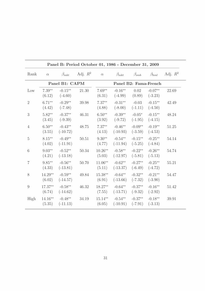
Panel B: Period October 01, 1986 - December 31, 2009
Rank α βmkt Adj. R2 α βmkt βsmb βhml Adj. R2
Panel B1: CAPM Panel B2: Fama-French
Low 7.39∗∗ -0.15∗∗ 21.30 7.69∗∗ -0.16∗∗ 0.02 -0.07∗∗ 22.69(6.12) (-4.60) (6.31) (-4.99) (0.89) (-3.23)
2 6.71∗∗ -0.29∗∗ 39.98 7.37∗∗ -0.31∗∗ -0.03 -0.15∗∗ 42.49(4.42) (-7.48) (4.88) (-8.00) (-1.11) (-4.50)
3 5.82∗∗ -0.37∗∗ 46.31 6.50∗∗ -0.39∗∗ -0.05∗ -0.15∗∗ 48.24(3.45) (-9.39) (3.92) (-9.72) (-1.95) (-4.15)
4 6.50∗∗ -0.43∗∗ 48.75 7.37∗∗ -0.46∗∗ -0.09∗∗ -0.19∗∗ 51.25(3.55) (-10.72) (4.13) (-10.93) (-3.59) (-4.53)
5 8.15∗∗ -0.49∗∗ 50.51 9.30∗∗ -0.54∗∗ -0.15∗∗ -0.25∗∗ 54.14(4.02) (-11.91) (4.77) (-11.94) (-5.25) (-4.84)
6 9.03∗∗ -0.52∗∗ 50.34 10.26∗∗ -0.58∗∗ -0.22∗∗ -0.26∗∗ 54.74(4.21) (-13.18) (5.03) (-12.97) (-5.81) (-5.13)
7 9.85∗∗ -0.56∗∗ 50.70 11.06∗∗ -0.62∗∗ -0.27∗∗ -0.25∗∗ 55.21(4.33) (-13.81) (5.11) (-13.37) (-6.49) (-4.72)
8 14.29∗∗ -0.59∗∗ 49.84 15.38∗∗ -0.64∗∗ -0.32∗∗ -0.21∗∗ 54.47(6.02) (-14.57) (6.91) (-13.66) (-7.32) (-3.90)
9 17.37∗∗ -0.58∗∗ 46.32 18.27∗∗ -0.64∗∗ -0.37∗∗ -0.16∗∗ 51.42(6.74) (-14.62) (7.55) (-13.71) (-9.32) (-2.92)
High 14.16∗∗ -0.48∗∗ 34.19 15.14∗∗ -0.54∗∗ -0.37∗∗ -0.18∗∗ 39.91(5.35) (-11.13) (6.05) (-10.91) (-7.91) (-3.13)
31
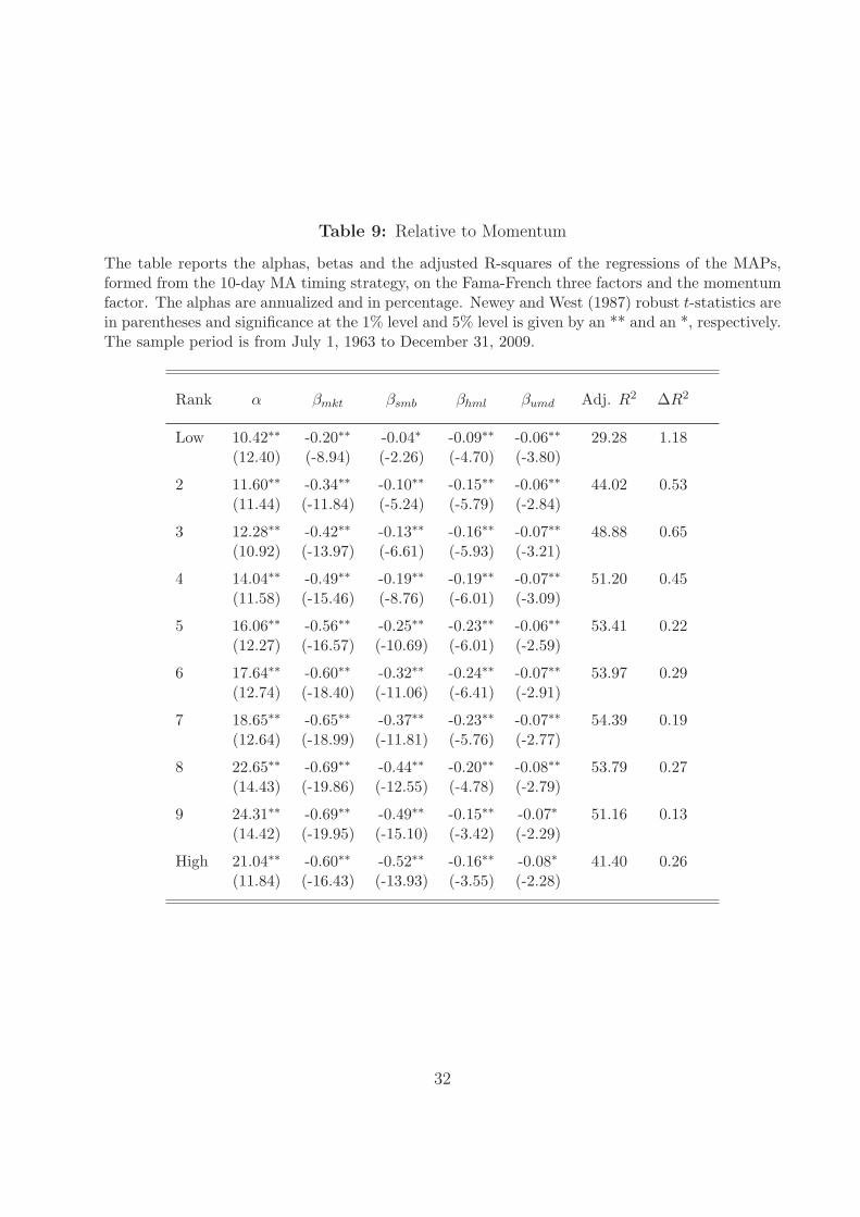
Table 9: Relative to Momentum
The table reports the alphas, betas and the adjusted R-squares of the regressions of the MAPs,formed from the 10-day MA timing strategy, on the Fama-French three factors and the momentumfactor. The alphas are annualized and in percentage. Newey and West (1987) robust t-statistics arein parentheses and significance at the 1% level and 5% level is given by an ** and an *, respectively.The sample period is from July 1, 1963 to December 31, 2009.
Rank α βmkt βsmb βhml βumd Adj. R2 ∆R2
Low 10.42∗∗ -0.20∗∗ -0.04∗ -0.09∗∗ -0.06∗∗ 29.28 1.18(12.40) (-8.94) (-2.26) (-4.70) (-3.80)
2 11.60∗∗ -0.34∗∗ -0.10∗∗ -0.15∗∗ -0.06∗∗ 44.02 0.53(11.44) (-11.84) (-5.24) (-5.79) (-2.84)
3 12.28∗∗ -0.42∗∗ -0.13∗∗ -0.16∗∗ -0.07∗∗ 48.88 0.65(10.92) (-13.97) (-6.61) (-5.93) (-3.21)
4 14.04∗∗ -0.49∗∗ -0.19∗∗ -0.19∗∗ -0.07∗∗ 51.20 0.45(11.58) (-15.46) (-8.76) (-6.01) (-3.09)
5 16.06∗∗ -0.56∗∗ -0.25∗∗ -0.23∗∗ -0.06∗∗ 53.41 0.22(12.27) (-16.57) (-10.69) (-6.01) (-2.59)
6 17.64∗∗ -0.60∗∗ -0.32∗∗ -0.24∗∗ -0.07∗∗ 53.97 0.29(12.74) (-18.40) (-11.06) (-6.41) (-2.91)
7 18.65∗∗ -0.65∗∗ -0.37∗∗ -0.23∗∗ -0.07∗∗ 54.39 0.19(12.64) (-18.99) (-11.81) (-5.76) (-2.77)
8 22.65∗∗ -0.69∗∗ -0.44∗∗ -0.20∗∗ -0.08∗∗ 53.79 0.27(14.43) (-19.86) (-12.55) (-4.78) (-2.79)
9 24.31∗∗ -0.69∗∗ -0.49∗∗ -0.15∗∗ -0.07∗ 51.16 0.13(14.42) (-19.95) (-15.10) (-3.42) (-2.29)
High 21.04∗∗ -0.60∗∗ -0.52∗∗ -0.16∗∗ -0.08∗ 41.40 0.26(11.84) (-16.43) (-13.93) (-3.55) (-2.28)
32
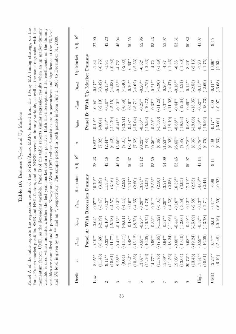
Table
10:
Busi
nes
sC
ycl
esan
dU
pM
arke
ts
Pan
elA
ofth
eta
ble
repo
rts
the
regr
essi
onre
sult
sof
the
NY
SE/A
mex
MA
Ps,
form
edfr
omth
e10
-day
MA
tim
ing
stra
tegy
,on
the
Fam
a-Fr
ench
mar
ket
port
folio
,SM
Ban
dH
ML
fact
ors,
and
anN
BE
Rre
cess
ion
dum
my
vari
able
,as
wel
las
the
sam
ere
gres
sion
wit
hth
em
omen
tum
fact
or,U
MD
,as
the
depe
nden
tva
riab
le.
Pan
elB
ofth
eta
ble
repo
rts
sim
ilar
regr
essi
onre
sult
sw
hen
anup
mar
ket
dum
my
vari
able
isus
edw
hich
indi
cate
sw
heth
erth
ela
stye
arm
arke
tre
turn
ispo
siti
ve.
Bot
hth
ein
terc
epts
and
the
coeffi
cien
tson
the
dum
my
vari
able
sar
ean
nual
ized
and
inpe
rcen
tage
.N
ewey
and
Wes
t(1
987)
robu
stt-
stat
isti
csar
ein
pare
nthe
ses
and
sign
ifica
nce
atth
e1%
leve
lan
d5%
leve
lis
give
nby
an**
and
an*,
resp
ecti
vely
.T
hesa
mpl
epe
riod
inbo
thpa
nels
isfr
omJu
ly1,
1963
toD
ecem
ber
31,20
09.
Dec
ileα
βm
kt
βsm
bβ
hm
lR
eces
sion
Adj
.R
2α
βm
kt
βsm
bβ
hm
lU
pM
arke
tA
dj.
R2
Pan
elA
:W
ith
Rec
essi
onD
um
my
Pan
elB
:W
ith
Up
Mar
ket
Dum
my
Low
8.05∗∗
-0.1
9∗∗
-0.0
4∗-0
.07∗∗
10.7
0∗∗
28.2
310
.82∗∗
-0.1
9∗∗
-0.0
4∗-0
.07∗∗
-1.3
227
.90
(11.
46)
(-8.
69)
(-2.
19)
(-3.
47)
(3.3
9)(7
.02)
(-8.
64)
(-2.
19)
(-3.
42)
(-0.
76)
29.
11∗∗
-0.3
3∗∗
-0.1
0∗∗
-0.1
3∗∗
11.3
3∗∗
43.4
612
.44∗∗
-0.3
3∗∗
-0.1
0∗∗
-0.1
3∗∗
-1.9
443
.23
(10.
61)
(-11
.77)
(-5.
18)
(-4.
57)
(3.1
6)(6
.42)
(-11
.70)
(-5.
15)
(-4.
53)
(-0.
92)
39.
68∗∗
-0.4
1∗∗
-0.1
3∗∗
-0.1
3∗∗
11.0
6∗∗
48.1
915
.06∗∗
-0.4
1∗∗
-0.1
3∗∗
-0.1
3∗∗
-4.7
6∗48
.04
(9.6
4)(-
13.7
7)(-
6.61
)(-
4.44
)(2
.92)
(7.0
1)(-
13.7
1)(-
6.58
)(-
4.40
)(-
2.03
)4
11.3
2∗∗
-0.4
8∗∗
-0.1
8∗∗
-0.1
6∗∗
11.7
7∗∗
50.6
718
.14∗∗
-0.4
8∗∗
-0.1
9∗∗
-0.1
6∗∗
-6.6
0∗∗
50.5
5(1
0.36
)(-
15.1
2)(-
8.75
)(-
4.65
)(2
.80)
(7.6
2)(-
15.0
4)(-
8.71
)(-
4.62
)(-
2.53
)5
13.0
7∗∗
-0.5
5∗∗
-0.2
5∗∗
-0.2
0∗∗
13.9
4∗∗
53.1
220
.22∗∗
-0.5
5∗∗
-0.2
5∗∗
-0.2
0∗∗
-6.5
2∗52
.96
(11.
26)
(-16
.05)
(-10
.74)
(-4.
79)
(3.0
5)(7
.84)
(-15
.93)
(-10
.72)
(-4.
75)
(-2.
33)
614
.77∗∗
-0.5
9∗∗
-0.3
2∗∗
-0.2
1∗∗
12.5
3∗∗
53.5
920
.36∗∗
-0.5
9∗∗
-0.3
2∗∗
-0.2
1∗∗
-4.7
253
.43
(11.
76)
(-17
.65)
(-11
.22)
(-5.
01)
(2.5
6)(6
.86)
(-17
.50)
(-11
.20)
(-4.
96)
(-1.
49)
715
.69∗∗
-0.6
4∗∗
-0.3
7∗∗
-0.2
0∗∗
13.2
1∗∗
54.0
921
.53∗∗
-0.6
4∗∗
-0.3
7∗∗
-0.2
0∗∗
-4.8
753
.97
(11.
56)
(-18
.24)
(-11
.96)
(-4.
52)
(2.5
8)(6
.92)
(-18
.10)
(-11
.92)
(-4.
47)
(-1.
46)
819
.05∗∗
-0.6
8∗∗
-0.4
4∗∗
-0.1
6∗∗
16.3
2∗∗
53.4
526
.65∗∗
-0.6
8∗∗
-0.4
4∗∗
-0.1
6∗∗
-6.5
553
.31
(13.
04)
(-19
.10)
(-12
.66)
(-3.
58)
(3.0
5)(7
.85)
(-18
.93)
(-12
.64)
(-3.
51)
(-1.
80)
920
.72∗∗
-0.6
8∗∗
-0.4
9∗∗
-0.1
2∗∗
17.1
9∗∗
50.9
729
.78∗∗
-0.6
8∗∗
-0.4
9∗∗
-0.1
2∗∗
-8.2
0∗50
.82
(13.
48)
(-19
.24)
(-15
.09)
(-2.
58)
(2.9
3)(8
.36)
(-19
.08)
(-15
.05)
(-2.
53)
(-2.
13)
Hig
h17
.81∗∗
-0.5
9∗∗
-0.5
2∗∗
-0.1
3∗∗
14.6
9∗∗
41.1
425
.78∗∗
-0.5
9∗∗
-0.5
2∗∗
-0.1
3∗∗
-7.2
041
.07
(10.
61)
(-16
.05)
(-13
.78)
(-2.
71)
(2.4
4)(6
.75)
(-15
.96)
(-13
.73)
(-2.
69)
(-1.
75)
UM
D12
.24∗∗
-0.1
7∗∗
-0.0
1-0
.41∗∗
-6.9
99.
113.
09-0
.17∗∗
-0.0
0-0
.41∗∗
10.8
6∗9.
45(6
.19)
(-5.
48)
(-0.
16)
(-6.
59)
(-0.
92)
(0.6
3)(-
5.60
)(-
0.07
)(-
6.68
)(2
.03)
33
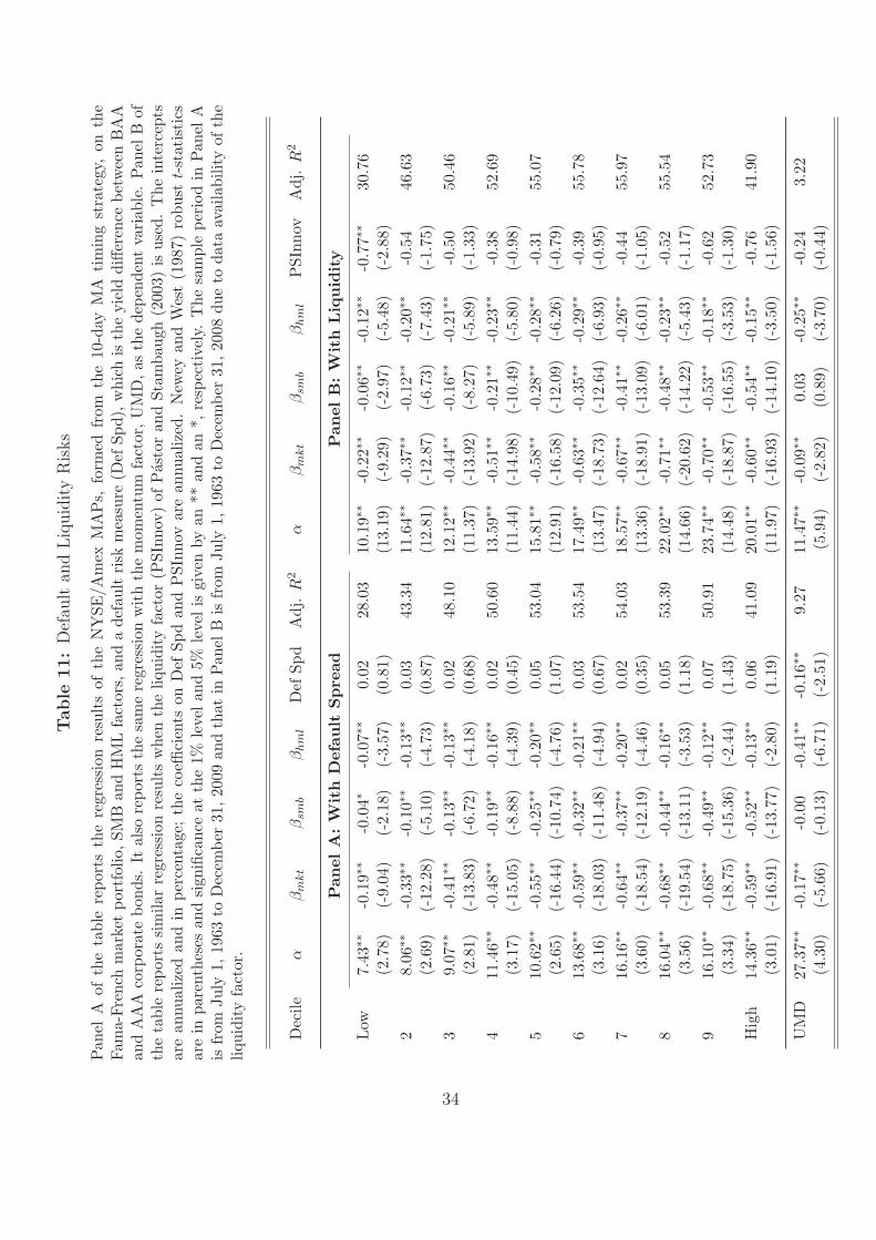
Table
11:
Def
ault
and
Liq
uid
ity
Ris
ks
Pan
elA
ofth
eta
ble
repo
rts
the
regr
essi
onre
sult
sof
the
NY
SE/A
mex
MA
Ps,
form
edfr
omth
e10
-day
MA
tim
ing
stra
tegy
,on
the
Fam
a-Fr
ench
mar
ket
port
folio
,SM
Ban
dH
ML
fact
ors,
and
ade
faul
tri
skm
easu
re(D
efSp
d),w
hich
isth
eyi
eld
diffe
renc
ebe
twee
nB
AA
and
AA
Aco
rpor
ate
bond
s.It
also
repo
rts
the
sam
ere
gres
sion
wit
hth
em
omen
tum
fact
or,U
MD
,as
the
depe
nden
tva
riab
le.
Pan
elB
ofth
eta
ble
repo
rts
sim
ilar
regr
essi
onre
sult
sw
hen
the
liqui
dity
fact
or(P
SInn
ov)
ofP
asto
ran
dSt
amba
ugh
(200
3)is
used
.T
hein
terc
epts
are
annu
aliz
edan
din
perc
enta
ge;
the
coeffi
cien
tson
Def
Spd
and
PSI
nnov
are
annu
aliz
ed.
New
eyan
dW
est
(198
7)ro
bust
t-st
atis
tics
are
inpa
rent
hese
san
dsi
gnifi
canc
eat
the
1%le
velan
d5%
leve
lis
give
nby
an**
and
an*,
resp
ecti
vely
.T
hesa
mpl
epe
riod
inPan
elA
isfr
omJu
ly1,
1963
toD
ecem
ber
31,2
009
and
that
inPan
elB
isfr
omJu
ly1,
1963
toD
ecem
ber
31,2
008
due
toda
taav
aila
bilit
yof
the
liqui
dity
fact
or.
Dec
ileα
βm
kt
βsm
bβ
hm
lD
efSp
dA
dj.
R2
αβ
mkt
βsm
bβ
hm
lP
SInn
ovA
dj.
R2
Pan
elA
:W
ith
Def
ault
Spre
adPan
elB
:W
ith
Liq
uid
ity
Low
7.43∗∗
-0.1
9∗∗
-0.0
4∗-0
.07∗∗
0.02
28.0
310
.19∗∗
-0.2
2∗∗
-0.0
6∗∗
-0.1
2∗∗
-0.7
7∗∗
30.7
6(2
.78)
(-9.
04)
(-2.
18)
(-3.
57)
(0.8
1)(1
3.19
)(-
9.29
)(-
2.97
)(-
5.48
)(-
2.88
)2
8.06∗∗
-0.3
3∗∗
-0.1
0∗∗
-0.1
3∗∗
0.03
43.3
411
.64∗∗
-0.3
7∗∗
-0.1
2∗∗
-0.2
0∗∗
-0.5
446
.63
(2.6
9)(-
12.2
8)(-
5.10
)(-
4.73
)(0
.87)
(12.
81)
(-12
.87)
(-6.
73)
(-7.
43)
(-1.
75)
39.
07∗∗
-0.4
1∗∗
-0.1
3∗∗
-0.1
3∗∗
0.02
48.1
012
.12∗∗
-0.4
4∗∗
-0.1
6∗∗
-0.2
1∗∗
-0.5
050
.46
(2.8
1)(-
13.8
3)(-
6.72
)(-
4.18
)(0
.68)
(11.
37)
(-13
.92)
(-8.
27)
(-5.
89)
(-1.
33)
411
.46∗∗
-0.4
8∗∗
-0.1
9∗∗
-0.1
6∗∗
0.02
50.6
013
.59∗∗
-0.5
1∗∗
-0.2
1∗∗
-0.2
3∗∗
-0.3
852
.69
(3.1
7)(-
15.0
5)(-
8.88
)(-
4.39
)(0
.45)
(11.
44)
(-14
.98)
(-10
.49)
(-5.
80)
(-0.
98)
510
.62∗∗
-0.5
5∗∗
-0.2
5∗∗
-0.2
0∗∗
0.05
53.0
415
.81∗∗
-0.5
8∗∗
-0.2
8∗∗
-0.2
8∗∗
-0.3
155
.07
(2.6
5)(-
16.4
4)(-
10.7
4)(-
4.76
)(1
.07)
(12.
91)
(-16
.58)
(-12
.09)
(-6.
26)
(-0.
79)
613
.68∗∗
-0.5
9∗∗
-0.3
2∗∗
-0.2
1∗∗
0.03
53.5
417
.49∗∗
-0.6
3∗∗
-0.3
5∗∗
-0.2
9∗∗
-0.3
955
.78
(3.1
6)(-
18.0
3)(-
11.4
8)(-
4.94
)(0
.67)
(13.
47)
(-18
.73)
(-12
.64)
(-6.
93)
(-0.
95)
716
.16∗∗
-0.6
4∗∗
-0.3
7∗∗
-0.2
0∗∗
0.02
54.0
318
.57∗∗
-0.6
7∗∗
-0.4
1∗∗
-0.2
6∗∗
-0.4
455
.97
(3.6
0)(-
18.5
4)(-
12.1
9)(-
4.46
)(0
.35)
(13.
36)
(-18
.91)
(-13
.09)
(-6.
01)
(-1.
05)
816
.04∗∗
-0.6
8∗∗
-0.4
4∗∗
-0.1
6∗∗
0.05
53.3
922
.02∗∗
-0.7
1∗∗
-0.4
8∗∗
-0.2
3∗∗
-0.5
255
.54
(3.5
6)(-
19.5
4)(-
13.1
1)(-
3.53
)(1
.18)
(14.
66)
(-20
.62)
(-14
.22)
(-5.
43)
(-1.
17)
916
.10∗∗
-0.6
8∗∗
-0.4
9∗∗
-0.1
2∗∗
0.07
50.9
123
.74∗∗
-0.7
0∗∗
-0.5
3∗∗
-0.1
8∗∗
-0.6
252
.73
(3.3
4)(-
18.7
5)(-
15.3
6)(-
2.44
)(1
.43)
(14.
48)
(-18
.87)
(-16
.55)
(-3.
53)
(-1.
30)
Hig
h14
.36∗∗
-0.5
9∗∗
-0.5
2∗∗
-0.1
3∗∗
0.06
41.0
920
.01∗∗
-0.6
0∗∗
-0.5
4∗∗
-0.1
5∗∗
-0.7
641
.90
(3.0
1)(-
16.9
1)(-
13.7
7)(-
2.80
)(1
.19)
(11.
97)
(-16
.93)
(-14
.10)
(-3.
50)
(-1.
56)
UM
D27
.37∗∗
-0.1
7∗∗
-0.0
0-0
.41∗∗
-0.1
6∗∗
9.27
11.4
7∗∗
-0.0
9∗∗
0.03
-0.2
5∗∗
-0.2
43.
22(4
.30)
(-5.
66)
(-0.
13)
(-6.
71)
(-2.
51)
(5.9
4)(-
2.82
)(0
.89)
(-3.
70)
(-0.
44)
34