Embed Size (px)
Citation preview

A New Approach of Using Levy Processes for Determining
High-Frequency Value at Risk Predictions
Wei Sun
Institute for Statistics and Mathematical Economics
University of Karlsruhe, Germany
Svetlozar Rachev
Institute for Statistics and Mathematical Economics
University of Karlsruhe, Germany
and
Department of Statistics and Applied Probability
University of California, Santa Barbara, USA
Frank J. Fabozzi∗
Yale School of Management
Yale University, USA†
∗Corresponding author: Frank J. Fabozzi, 858 Tower View Circle, New Hope, PA 18938, U.S.A. Email:
[email protected].†Acknowledgment: W. Sun’s research was supported by grants from the Deutschen Forschungsgemeinschaft and Chinese
Government Award for Outstanding Ph.D Students Abroad 2006 (No. 2006-180). S. Rachev’s research was supported by
grants from Division of Mathematical, Life and Physical Science, College of Letters and Science, University of California,
Santa Barbara, and the Deutschen Forschungsgemeinschaft.
1

A New Approach of Using Levy Processes for Determining High-FrequencyValue at Risk Predictions
Abstract
A new approach for using Levy processes to compute value at risk (VaR) using high-frequency datais presented in this paper. The approach is a parametric model using an ARMA(1,1)-GARCH(1,1)model where the tail events are modeled using the fractional Levy stable noise and Levy stabledistribution. Using high-frequency data for the German DAX Index, the VaR estimates from thisapproach are compared to those of a standard nonparametric estimation method that captures theempirical distribution function, and with models where tail events are modeled using Gaussian dis-tribution and fractional Gaussian noise. The results suggest that the proposed parametric approachyields superior predictive performance.
Key Words: Fractional Gaussian noise, Fractional Levy stable noise, High-frequency data, Levystable distribution, Value at Risk
JEL Classification: C15, C46, C52, G15
2
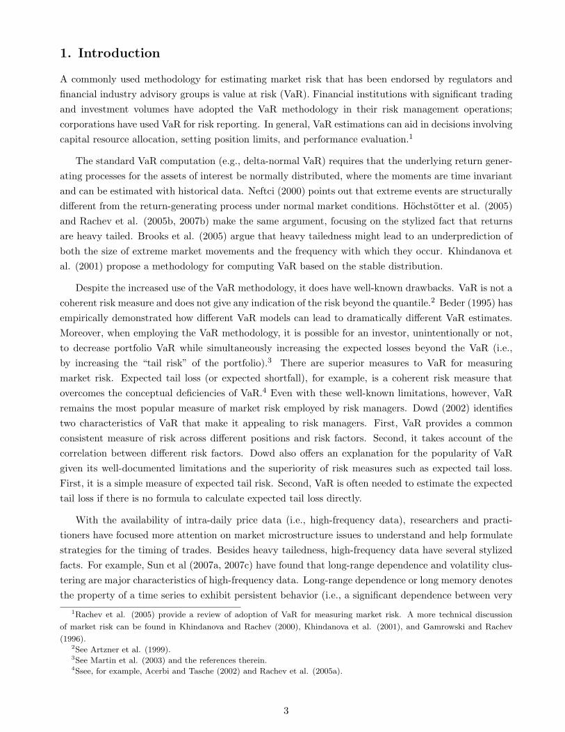
1. Introduction
A commonly used methodology for estimating market risk that has been endorsed by regulators andfinancial industry advisory groups is value at risk (VaR). Financial institutions with significant tradingand investment volumes have adopted the VaR methodology in their risk management operations;corporations have used VaR for risk reporting. In general, VaR estimations can aid in decisions involvingcapital resource allocation, setting position limits, and performance evaluation.1
The standard VaR computation (e.g., delta-normal VaR) requires that the underlying return gener-ating processes for the assets of interest be normally distributed, where the moments are time invariantand can be estimated with historical data. Neftci (2000) points out that extreme events are structurallydifferent from the return-generating process under normal market conditions. Hochstotter et al. (2005)and Rachev et al. (2005b, 2007b) make the same argument, focusing on the stylized fact that returnsare heavy tailed. Brooks et al. (2005) argue that heavy tailedness might lead to an underprediction ofboth the size of extreme market movements and the frequency with which they occur. Khindanova etal. (2001) propose a methodology for computing VaR based on the stable distribution.
Despite the increased use of the VaR methodology, it does have well-known drawbacks. VaR is not acoherent risk measure and does not give any indication of the risk beyond the quantile.2 Beder (1995) hasempirically demonstrated how different VaR models can lead to dramatically different VaR estimates.Moreover, when employing the VaR methodology, it is possible for an investor, unintentionally or not,to decrease portfolio VaR while simultaneously increasing the expected losses beyond the VaR (i.e.,by increasing the “tail risk” of the portfolio).3 There are superior measures to VaR for measuringmarket risk. Expected tail loss (or expected shortfall), for example, is a coherent risk measure thatovercomes the conceptual deficiencies of VaR.4 Even with these well-known limitations, however, VaRremains the most popular measure of market risk employed by risk managers. Dowd (2002) identifiestwo characteristics of VaR that make it appealing to risk managers. First, VaR provides a commonconsistent measure of risk across different positions and risk factors. Second, it takes account of thecorrelation between different risk factors. Dowd also offers an explanation for the popularity of VaRgiven its well-documented limitations and the superiority of risk measures such as expected tail loss.First, it is a simple measure of expected tail risk. Second, VaR is often needed to estimate the expectedtail loss if there is no formula to calculate expected tail loss directly.
With the availability of intra-daily price data (i.e., high-frequency data), researchers and practi-tioners have focused more attention on market microstructure issues to understand and help formulatestrategies for the timing of trades. Besides heavy tailedness, high-frequency data have several stylizedfacts. For example, Sun et al (2007a, 2007c) have found that long-range dependence and volatility clus-tering are major characteristics of high-frequency data. Long-range dependence or long memory denotesthe property of a time series to exhibit persistent behavior (i.e., a significant dependence between very
1Rachev et al. (2005) provide a review of adoption of VaR for measuring market risk. A more technical discussion
of market risk can be found in Khindanova and Rachev (2000), Khindanova et al. (2001), and Gamrowski and Rachev
(1996).2See Artzner et al. (1999).3See Martin et al. (2003) and the references therein.4Ssee, for example, Acerbi and Tasche (2002) and Rachev et al. (2005a).
3

distant observations and a pole in the neighborhood of the zero frequency of its spectrum.5 Long-rangedependence time series typically exhibit self-similarity. The stochastic processes with self-similarity areinvariant in distribution with respect to changes of time and space scale.6
In this paper, we propose an approach for calculating VaR with high-frequency data. The approachutilizes the ARMA(1,1)-GARCH(1,1) model with Levy stable processes for computing VaR. The em-pirical evidence we present suggests that this approach outperforms three other parametric modelsinvestigated. Our findings are consistent with the empirical results reported in Sun et al. (2007a) thatan ARMA(1,1)-GARCH(1,1) model with Levy stable noise residuals exhibits superior performance inmodeling high-frequency stock returns.
We have organized the paper as follows. In Section 2, we introduce the methodology for estimatingand evaluating parametric and nonparametric VaR. In Section 3, we specify the three Levy familymodels investigated in our study (the Levy stable distribution, fractional Gaussian noise, and Levyfractional stable noise) utilized in modeling the residuals distribution for computing parametric VaRwith the help of the ARMA(1,1)-GARCH(1,1) model. In this section, we discuss the financial meaningof using these models. The study’s data and empirical methodology are described in Section 4. InSection 5, we compare the performance of our VaR models based on high-frequency data at 1-minutelevel for the German DAX index. We summarize our conclusions in Section 6.
2. Value at Risk
In mathematical terms, VaR is defined as follows. Given α ∈ (0, 1], R is a random gain or loss of aninvestment over a certain period. VaR of a random variable R at level of α is the absolute value ofthe worst loss not to be exceeded with a probability of at least α, more formally, if α-quantile of R isqα(R) = inf{r ∈ < : P [R ≤ r] ≥ α}, the VaR at confidence level α of R is V aRα(R) = qα(−R).
2.1 Non-parametric Approach of VaR Estimation
VaR is in fact the quantile of loss distribution for an asset. Consequently, the estimation of VaR isindeed the estimation of the loss distribution. The kernel estimator is the basic methodology employedto estimate the density (see Silverman (1986)). If random variable X has density f(x), then
f(x) = lima→0
12a
P (x− a < X < x + a) .
By counting the proportion of sampling observations falling in the interval of (x−a, x+a), the probabilityP (x− a < X < x + a) can be estimated for any given a. Defining the kernel function K for∫ ∞
−∞K(x)d(x) = 1,
5Baillie (1996) provides a survey of the major econometric research on long-range dependence processes, fractional
integration, and applications in economics and finance. Doukhan et al. (2003) and Robinson (2003) provide a comprehen-
sive review of the studies on long-range dependence. Bhansali and Kokoszka (2006) review recent research on long-range
dependence time series. Recent theoretical and empirical research on long-range dependence in economics and finance
is provided by Rangarajan and Ding (2006) and Teyssiere and Kirman (2006). Sun et al. (2007c) provide a review of
long-range dependence research based on using intra-daily data.6See Samorodnisky and Taqqu (1994) and Doukhan et al. (2003).
4

in which K(x) usually but not always is regarded as a symmetric probability density function (e.g.,normal density), the kernel estimator is defined by
f(x) =1na
n∑i=1
K
(x−Xi
a
),
where a is the window width and n is sample size. The kernel estimator can be reviewed as a sum ofbumps placed at the observations Xi. Kernel function K(x) determines the shape of the bumps andwindow width a determines the width of the bumps. Silverman (1986) shows that
aopt = n−1/5 k−2/52
(∫f ′′(x)2dx
)−1/5 (∫K(t)2dt
)1/5
and the optimal solution is given by the Epanechnikov kernel KE(x):
KE(x) =
3
4√
5(1− x2
5 ), −√
5 ≤ x ≤√
5
0, else
A slight drawback suffered by the kernel estimator is the inefficiency in dealing with long-tailed distri-butions. Since across the whole sample the window width is fixed, a good degree of smoothing overthe center of the distribution will often leave spurious noise in the tail (see Silverman (1986) and Dowd(2005)). Silverman (1986) offers several solutions such as the nearest neighbor method and variablekernel method. For the nearest neighbor method, the window width placed on an observation dependson the distance between that observation and its nearest neighbors. For the variable kernel estimator,the density f(x) is estimated as follows
f(x) =1n
n∑i=1
1ahi,k
K
(x−Xi
ahi,k
),
where hi,k is the distance between Xi and the kth nearest of the other data points. The window widthof the kernel placed on Xi is proportional to hi,k, therefore flatter kernels will be placed on more sparsedata.
2.2 Parametric Approach of VaR Estimation
The parametric approach for VaR estimation is based on the assumption that the financial returns Rt
are a function of two components µt and εt (i.e., Rt = f(µt, εt)). Rt can be regarded as a function ofεt conditional on a given µt; typically this function takes a simple linear form Rt = µt + εt = µt + σtut.Usually µt is referred to as the location component and σt the scale component. ut is an independentand identically distributed (i.i.d.) random variable that follows a probability density function fu. VaRbased on information up to time t is then
˜V aRt := qα(Rt) = −µt + σ qα(u),
where qα(u) is the α-quantile implied by fu.
Unconditional parametric approaches set µt and σt as constants, therefore the returns Rt are i.i.drandom variables with density σ−1fu(σ−1(Rt−µ)). Conditional parametric approaches set location com-ponent and scale component as functions not constants. The typical time-varying conditional location
5

setting is the ARMA(r, m) processes. That is, the conditional mean equation is:
µt = α0 +r∑
i=1
αi Rt−i +m∑
j=1
βjεt−j .
The typical time-varying conditional variance setting is GARCH(p,q) processes given by
σ2t = κ +
p∑i=1
γi σ2t−i +
q∑j=1
θj ε2t−j .
Different distributional assumptions for the innovation distribution fu can be made. In the empir-ical analysis below, distributional assumptions analyzed for the parametric approaches are the normaldistribution, fractional Gaussian noise, fractional Levy stable noise, and Levy stable distribution.
2.3 Evaluation of VaR Estimators
Backtesting is the usual method to evaluate the VaR estimators and its forecasting quality. It canbe performed for in-sample estimation evaluation and for out-of-sample interval forecasting evaluation.The backtesting is based on the indicator function It which is defined as It(α) = I(rt < −V aRt(α)).The indicator function shows violations of the quantiles of the loss distribution. Then the process{It}t∈T is a process of i.i.d Bernoulli variables with violation probability 1 − α. Christoffersen (1998)shows that evaluating the accuracy of VaR can be reduced to checking whether (1) the number ofviolations is correct on average and (2) the pattern of violations is consistent with i.i.d processes. Inanother word, an accurate VaR measure should satisfy both the unconditional coverage property andindependent property. The unconditional coverage property means that the probability of realization ofa loss in excess of the estimated V aRt(α) must be exactly α% (i.e., P (It(α) = 1) = α). The independentproperty means that previous VaR violations do not presage future VaR violations.
Kupiec (1995) proposes a frequency of failures test that checks how many time an estimated VaRis violated in a given time period. If the observed frequency of failures of the estimated VaR differssignificantly from α × 100%, the underlying risk measure is less reliable. The shortcoming of thebacktesting proposed by Kupiec is that it fails to focus on the independence property. In order todetect violations of the independence property of an estimated VaR measure, say, It(α), Christoffersen(1998) suggests the Markov test. This test detects whether the likelihood of a VaR violation dependson another VaR violation occurring in the previous time period. The assumption underlying this test isthat VaR is adequate to capture the risk factors and previous VaR violations cannot cause a future VaRviolation; that is, the chance of violating the current period’s VaR should not depend on whether theprevious period’s VaR was violated and the chance of violating current period’s VaR should not influencenext period’s violation. Campbell (2005) provides a review of backtests examining the adequacy of VaRmodels.
6

3. Levy Processes with Financial Implementation
Levy processes7 have become increasingly popular in mathematical finance because they can describethe observed behavior of financial markets in a more accurate way than other processes typically usedsuch as the normal distribution. They capture jumps, heavy-tails, and skewness observed in the marketfor asset price processes. Moreover, Levy processes provide the appropriate option pricing frameworkto model implied volatilities across strike prices and across maturities with respect to the “risk-neutral”assumption.
When investors select stocks and put them together to form a portfolio, they use the normal distrib-ution to calculate risk by first calculating the beta, a measure of a particular stock’s volatility in relationto the overall market, for every investment in the portfolio. Unfortunately, the normal distribution isnot adequate enough to capture market characteristics (see, for example, Rachev and Mittnik (2000)).Some recurring themes in the pattern of stock returns such as volatility clustering have been observed.So how might portfolio managers better measure risk if stock returns followed a pattern that is not anormal distribution? Mandelbrot makes a few suggestions for measuring market risk based on the toolsof fractal geometry. Among the more alluring are the “H” (Hurst) index, which is an indication of the“persistence” or trend that affects a stock’s return. Roughly speaking, a high “H” value could indicatecrowd behavior of stock returns, while a low “H” value may indicate a more random “classic” marketforce (see Mandelbrot (1997, 2005) and Sun et al. (2007a)). The Levy stable distribution and Levyfractional stable processes provide a good solution to capture observed market characteristics such asvolatility clustering, heavier tails than the normal distribution, and persistence of stock returns.
Moreover, fractal processes have a close relationship to the fractal market hypothesis (FMH), whichstates that (1) a market consists of many investors with different investment horizons and (2) theinformation set that is important to each investment horizon is different. As long as the market maintainsthis fractal structure, with no characteristic time scale, the market remains stable. When the market’sinvestment horizon becomes uniform, the market becomes unstable because everyone is trading basedupon the same information set (see Peters (1989, 1994)). The roughness induced by the fractal markethypothesis can be modeled by fractal processes (see Mandelbrot (1997, 2005)).
4. Data
To test the relative performance of the models we presented in this paper, we use high-frequency datafor the Deutsche Aktien Xchange (DAX) index from January 2 to September 30, 2006 that were aggre-gated to the 1-minute frequency level.8 The aggregation algorithm is based on the linear interpolationmethodology introduced by Wasserfallen and Zimmermann (1995). That is, given an inhomogeneousseries with times ti and values ϕi = ϕ(ti), the index i identifies the irregularly spaced sequence. Thetarget homogeneous time series is given at times t0 + j∆t with fixed time interval ∆t starting at t0.
7We review the definition of Levy processes as well as one specific form (the Levy fractional stable motion) and two
extensions of infinitely divisible distributions (the Levy stable distribution and fractional Brownian motion) that we use
in the appendix to this paper. Further details can be found in Sato (1999).8The DAX index is a stock market index whose components include 30 blue chip German stocks that are traded on the
Frankfurt Stock Exchange. Starting in 2006, the DAX index is calculated every second. In our original dataset, the DAX
index is sampled at the one-second level.
7
The index j identifies the regularly spaced sequence. The time t0 + j∆t is bounded by two times ti ofthe irregularly spaced series, I = max( i |ti ≤ t0 + j∆t) and tI ≤ t0 + j∆t > tI+1. Data are interpolatedbetween tI and tI+1. The linear interpolation shows that
ϕ(t0 + j∆t) = ϕI +t0 + j∆t− tI
tI+1 − tI(ϕI+1 − ϕI).
Dacorogna et al. (2001) point out that linear interpolation relies on the forward point of time andMuller et al. (1990) suggests that linear interpolation is an appropriate method for stochastic processeswith i.i.d. increments.
Empirical evidence has identified the seasonality in high-frequency data. Engle and Russell (1998)and other researchers adopt several methods to adjust the seasonal effect in data in order to remove suchdisturbance. In our study, seasonality is treated as one type of self-similarity which can be captured byfactional processes that we employed. Consequently, it is not necessary to adjust for the seasonal effectin the data.
In previous studies that have studied the computing of VaR, low-frequency data typically have beenused. Because stock indexes change their composition quite often over time, it is difficult to identifythe impact of these changes in composition when analyzing the return history of stock indexes usinglow-frequency data. Dacorogna et al. (2001) call this phenomenon the “breakdown of the permanencehypothesis”. In order to overcome this problem, we use high-frequency data in our study. In addition,because more and more day trading strategies are being employed by practitioners, measuring the riskover a short time interval is of importance to practitioners. Therefore, using high-frequency data tocompute VaR has practical importance.
Employing high-frequency data has several advantages compared with low-frequency data. First,with a very large number of observations, high-frequency data offers a higher level of statistical signif-icance. Second, high-frequency data are gathered at a low level of aggregation, thereby capturing theheterogeneity of players in financial markets. These players should be properly modeled in order to makevalid inferences about market movements. Low-frequency data such as daily or weekly data aggregatethe heterogeneity in a smoothing way. As a result, many of the movements in the same direction arestrengthened and those in the opposite direction cancelled in the process of aggregation. The aggregatedseries generally show smoother style than their components. The relationships between the observationsin these aggregated series often exhibit greater smoothness than their components. For example, a curveexhibiting a one-week market movement based on daily return data might be a line with a couple ofkinks. The smooth line segment masks the intra-daily fluctuation of the market. But high-frequencydata can reflect such intra-daily fluctuations and the intra-daily factors that influence the risks canbe taken into account. Third, using high-frequency data in computing VaR in an equity market canconsider both microstructure risk effects and macroeconomic risk factors. This is because informationcontained in high-frequency data can be separated into a higher frequency part (i.e., the intra-dailyfluctuation) and a lower frequency part (i.e., low-frequency smoothness). The information provided bythe higher frequency part mirrors the microstructure effect of the equity markets and the information inthe lower frequency part shows the smoothed trend that is usually influenced by macroeconomic factorsin these markets.
Standard econometric techniques are based on homogeneous time series analysis. If a practitioner
8
uses analytic methods of homogeneous time series for inhomogeneous time series, the reliability of theresults will be doubtful. Aggregating inhomogeneous tick-by-tick data to the equally spaced (homoge-neous) time series is required. Engle and Russell (1998) argue that aggregating tick-by-tick data to afixed time interval, if a short time interval is chosen, there will be many intervals in which there is nonew information, and if choosing a wide interval, micro-structure features might be missing. Aıt-Sahalia(2005) suggests keeping the data at the ultimate frequency level. In our empirical study, intra-dailydata (which we refer to as high-frequency data in this paper) at the 1-minute level is aggregated fromtick-by-tick data to compute VaR for the models investigated.
5. Empirical study
An ARMA(1,1)-GARCH(1,1) model with different residuals (i.e., the normal distribution, the Levystable distribution, the Levy fractional stable noise, and the fraction Gaussian noise) is employedto compute VaR using the high-frequency DAX data described in Section 4. We will refer to theARMA(1,1)-GARCH(1,1) model as simply the “AG model”. The methodology for estimation and sim-ulation of the AG model with different residuals is explained in Sun et al. (2007a). We performed twoexperiments. In the first experiment, we calculate 95%-VaR values and 99%-VaR values for the entiredata sample. In the second experiment, we split the dataset into two subsets: an in-sample (training)set and an out-of-sample (forecasting) set. The purpose of this second experiment is mainly to checkthe predictive power of parametric VaR values computed from the training sample.
We compute the in-sample 95% VaR and 99% VaR for a horizon of six months. Our datasetcontains nine months of data. In order to ensure randomness of the data from which VaR is computed,after each computation, we shift the next starting point of the training dataset for VaR computationtwo weeks afterwards. Table 1 shows the results of the VaR value computed six times by the above-mentioned models for the in-sample estimation. The empirical VaR is computed using the nonparametricKernel estimator. Table 2 provides a comparison between the VaR values computed from the differentparametric AG models and the empirical VaR values. The results in this table indicate that the 95%VaR computed from the AG model with fractional stable noise has minimal absolute distance to theempirical value. However, the AG model with standard normal residuals has minimal absolute distanceto the empirical VaR value in computing the 99% VaR compared to the other alternatives. This resultsuggests that although the AG model with fractional Levy stable residuals provides a good modelingmechanism to capture the stylized facts observed from high-frequency data (see Sun et al. (2007a)), itis focusing on capturing long-term dependence of extreme events. In this case, the VaR value turns outto overestimate the VaR value if α is set too small.
In order to test the predictive power of the VaR value computed for each model, in our secondexperiment we test the following six predictions using a different length of time for the training andprediction datasets:
1. Training period is 6 months (236,160 data points) and one-step-ahead forecast for 6 months, 3months, 1 month, 1 week, 1 day and 1 hour;
2. Training period is 3 months (124,800 data points) and one-step-ahead forecast for 3 months, 1month, 1 week, 1 day and 1 hour;
9

3. Training period is 1 month (40,320 data points) and one-step-ahead forecast for 1 month, 1 week,1 day and 1 hour;
4. Training period is 1 week (9,600 data points) and one-step-ahead forecast for 1 week, 1 day and1 hour;
5. Training period is 1 day (1,920 data points) and one-step-ahead forecast for 1 day and 1 hour;
6. Training period is 1 hour(240 data points) and one-step-ahead forecast for 1 hour.
Tables 3 and 4 show the results for the 95% VaR and 99% VaR computations, respectively.
Table 5 shows the admissible VaR violations and violation frequencies based on the Kupiec test.Considering the admissible VaR violations and violation frequencies shown in Table 3 for the predictionof 95% VaR, the AG model with fractional stable noise performs better than the other alternatives.For the prediction of 99% VaR, although all computed VaR values turns out to be conservative, theAG model with standard normal distribution has the best performance because it has violations closeto the admissible VaR violations.
Backtesting is the typical method for evaluating VaR estimators and their forecasting performance.It can be performed for in-sample estimation evaluation and for out-of-sample interval forecasting evalua-tion. The backtesting is based on the indicator function It which is defined as It(α) = I(rt < −V aRt(α)).The indicator function shows violations of the quantiles of the loss distribution. Then the process {It}t∈T
is a process of i.i.d Bernoulli variables with violation probability 1 − α. Christoffersen (1998) showsthat evaluating the accuracy of VaR can be reduced to checking whether the number of violations iscorrect on average and the pattern of violations is consistent with i.i.d processes (see Section 2.3). Inanother words, an accurate VaR measure should satisfy both the unconditional coverage property andindependent property. The unconditional coverage property means that the probability of realization ofa loss in excess of the estimated V aRt(α) must be exactly α% (i.e., P (It(α) = 1) = α). The independentproperty means that previous VaR violations do not presage future VaR violations. Table 3 reportsthe p value for the Christoffersen test, where the null hypothesis is that the pattern of violations isconsistently independent.
By comparing the admissible VaR violations with the violation in our out-of-sample forecastingexperiment, we find that the parametric VaR values computed from the AG models provide a relativelyconservative risk measure for forecasting if the α is set too small for the training dataset used tocompute in-sample VaR. The reason is that given the model used for parametric VaR calculation iswell specified, the VaR values calculated from the in-sample dataset in which the data illustrate highvolatility or significant regime switching will provide a conservative prediction (over-prediction) for theout-of-sample (forecasting) dataset. If the out-of-sample (forecasting) dataset share similar trends asthose in the in-sample (training) dataset, the VaR value can provide adequate prediction with respectto the α level specified. If the in-sample dataset illustrate different trends in the out-of-sample dataset,particularly when regime switching is observed for the in-sample dataset to the out-of-sample dataset,the predictive power of the VaR value for the latter dataset will be reduced.
Table 6 reports the p-value for Christoffersen test. The results of this test suggest that the patternof violation of our parametric VaR in the out-of-sample forecasting is consistently independent. We can
10

observe that the VaR value calculated by the AG model with Levy stable and fractional Levy noiseperforms better than the alternative models because the p-values for rejecting the null hypothsis areless than that of the alternative models.
6. Conclusion
There is considerable interest in the computing of VaR for market risk management. Most modelsfollow the Gaussian distribution despite the overwhelming empirical evidence that fails to support thehypothesis that financial asset returns can be characterized as Gaussian random walks. There are anumber of arguments against both the Gaussian assumption and random walk assumption. One ofthe most compelling is that there exist fractals in financial markets. In this paper, we propose a newapproach for computing VaR. We test this approach using the DAX index at one minute frequency levelwith parametric models which capture stylized facts observated in high-frequency data, i.e., ARMA(1,1)-GARCH(1,1) model with Levy-type of residuals.
In our empirical analysis, we investigate both in-sample (training) performance and out-of-sample(forecasting) performance based on the Kupiec violation test and Christoffersen independent test. Ourempirical results show that the VaR calculated from the underlying models (i.e., AG model with residualsof Levy stable distribution and AG model with residuals of fractional Levy noise) performs better thanVaR calculated based on the alternative models (i.e., AG model with residuals of normal distributionand AG model with fractional Gaussian noise).
The empirical evidence based on out-of-sample forecasting suggests that VaR calculated by theunderlying models turns out to be conservative with respect to violation frequencies. However, theprediction power of parametric VaR is limited by the training dataset and our models focus on capturingconsistent extreme events. In order to make the VaR value less conservative, the underlying datagenerating processes should have tempered tails in their distributions.
11

Appendix
Levy Stable Distribution
The Levy stable distribution (sometimes referred to as α-stable distribution) has four parameters forcomplete description: an index of stability α ∈ (0, 2] (also called the tail index), a skewness parameterβ ∈ [−1, 1], a scale parameter γ > 0, and a location parameter ζ ∈ <. There is unfortunately noclosed-form expression for the density function and distribution function of a Levy stable distribution.Rachev and Mittnik (2000) give the definition for the Levy stable distribution: A random variable Xis said to have a Levy stable distribution if there are parameters 0 < α ≤ 2, −1 ≤ β ≤ 1, γ ≥ 0 and ζ
real such that its characteristic function has the following form:
E exp(iθX) =
{exp{−γα|θ|α(1− iβ(sin θ) tan πα
2 ) + iζθ}, if α 6= 1exp{−γ|θ|(1 + iβ 2
π (sin θ) ln |θ|) + iζθ}, if α = 1
and,
signθ =
1, if θ > 00, if θ = 0
−1, if θ < 0
For 0 < α < 1 and β = 1 or β = −1, the stable density is only for a half line.
Fractional Brownian Motion
For a given H ∈ (0, 1), there is basically a single Gaussian H-sssi 9 process, namely fractional Brownianmotion (fBm), first introduced by Kolmogorov (1940). Mandelbrot and Wallis (1968) and Taqqu (2003)define fBm as a Gaussian H-sssi process {BH(t)}t∈R with 0 < H < 1. Mandelbrot and van Ness (1968)define the stochastic representation
BH(t) :=1
Γ(H + 12)
(∫ 0
−∞[(t− s)H− 1
2 − (−s)H− 12 ]dB(s) +
∫ t
0(t− s)H− 1
2 dB(s))
,
where Γ(·) represents the Gamma function:
Γ(a) :=∫ ∞
0xa−1e−xdx,
and 0 < H < 1 is the Hurst parameter. The integrator B is ordinary Brownian motion. The principaldifference between fractional Brownian motion and ordinary Brownian motion is that the incrementsin Brownian motion are independent while in fractional Brownian motion they are dependent. Forfractional Brownian motion, Samorodnitsky and Taqqu (1994) define its increments {Yj , j ∈ Z} asfractional Gaussian noise (fGn), which is, for j = 0,±1,±2, ..., Yj = BH(j − 1)−BH(j).
9The abbreviation of “sssi” means self-similar stationary increments, if the exponent of self-similarity H is to be
emphasized, then “H-sssi” is adopted. Lamperti (1962) first introduced the semi-stable processes (which we today refer
to as self-similar processes). Let T be either R, R+ = {t : t ≥ 0} or {t : t > 0}. The real-valued process {X(t), t ∈ T} has
stationary increments if X(t + a) − X(a) has the same finite-dimensional distrituions for all a ≥ 0 and t ≥ 0. Then the
real-valued process {X(t), t ∈ T} is self-similar with exponent of self-similarity H for any a > 0, and d ≥ 1, t1, t2, ..., td ∈ T ,
satisfying: (X(at1), X(at2), ..., X(atd))d= (aHX(t1), a
HX(t2), ...aHX(td)).
12

Levy Stable Motion
The most commonly used is linear Levy fractional motion (also called linear fractional stable motion),{Lα,H(a, b; t), t ∈ (−∞,∞)}, which Samorodinitsky and Taqqu (1994) define as
Lα,H(a, b; t) :=∫ ∞
−∞fα,H(a, b; t, x)M(dx), (1)
where
fα,H(a, b; t, x) := a
((t− x)
H− 1α
+ − (−x)H− 1
α+
)+ b
((t− x)
H− 1α
− − (−x)H− 1
α−
), (2)
and a, b are real constants. |a|+ |b| > 1, 0 < α < 2, 0 < H < 1, H 6= 1/α, and M is an α-stable randommeasure on R with Lebesgue control measure and skewness intensity β(x), x ∈ (−∞,∞) satisfying:β(·) = 0 if α = 1. They define linear fractional stable noises expressed by Y (t), and Y (t) = Xt −Xt−1,
Y (t) = Lα,H(a, b; t)− Lα,H(a, b; t− 1) (3)
=∫
R
(a
[(t− x)
H− 1α
+ − (t− 1− x)H− 1
α+
]+ b
[(t− x)
H− 1α
− − (t− 1− x)H− 1
α−
])M(dx),
where Lα,H(a, b; t) is a linear fractional stable motion and M is a stable random measure with Lebesguecontrol measure given 0 < α < 2. Samorodinitsky and Taqqu (1994) show that the kernel fα,H(a, b; t, x)is d-self-similar with d = H − 1/α when Lα,H(a, b; t) is 1/α-self-similar. This implies H = d + 1/α (seeTaqqu and Teverovsky (1998) and Weron et al. (2005)).10 In this paper, if there is no special indication,the fractional stable noise (fsn) is generated from a linear fractional Levy motion.
10Some properties of these processes have been discussed in Mandelbrot and Van Ness (1968), Maejima (1983), Maejima
and Rachev (1987), Rachev and Mittnik (2000), Rachev and Samorodnitsky (2001), Samorodnitsky (1994, 1996, 1998),
Samorodinitsky and Taqqu (1994), and Cohen and Samorodnitsky (2006).
13

References
[1] Acerbi, C., D. Tasche (2002) On the coherence of expected shortfall. Journal of Banking and Finance 26: 1487-1503.
[2] Artzner, P., F. Delbaen, J. Eber, D. Heath (1999). Coherent measures of risk. Mathematical Finance 9: 203-228.
[3] Baillie, R.T. (1996). Long memory processes and fractional integration in econometrics. Journal of Econometrics
73(1): 5-59.
[4] Beder, T. (1995). VAR: seductive but dangerous. Financial Analysts Journal (51): 12-24.
[5] Bhansali, R.J., P.S. Kokoszaka (2006). Prediction of long-memory time series: a tutorial review. In G. Rangarajan
and M. Ding (eds.) Processes with Long-Range Correlations: Theory and Applications. Springer: New York.
[6] Brooks, C., A. D. Clare, J. Molle, G. Persand (2005). A comparison of extreme value theory approaches for deter-
mining value at risk. Journal of Empirical Finance 12: 339-352.
[7] Campbell, S.D. (2005). A review of backtesting and backtesting procedures. Finance and Economic Discussion Series,
Federal Reserve Board, Washington, D.C.
[8] Christoffersen, P. (1998). Evaluating interval forecasts. International Economic Review 39: 841-862.
[9] Cohen, S., G. Samorodnitsky (2006). Random rewards, fractional Brownian local times and stable self-similar
processes. The Annals of Applied Probability 16(3): 1432-1461.
[10] Doukhan, P., G. Oppenheim, M.S. Taqqu (2003). Theory and Applications of Long-Range Dependence, eds.,
Birkhauser: Boston.
[11] Dowd, K. (2002). Measuring Market Risk. John Wiley & Sons: Chichester.
[12] Fama, E. (1963). Mandelbrot and the stable Paretian hypothesis. Journal of Business 36: 420-429.
[13] Gamrowski, B., S. Rachev (1996). Testing the validity of value at risk measures. In C. Heyde et al. (eds) Applied
Probability.
[14] Hochstotter, M., S. Rachev, F. Fabozzi, F (2005). Distributional analysis of the stocks comprising the DAX 30.
Probability and Mathematical Statistics 25(2):363-383.
[15] Khindanova, I., S. Rachev (2000). Value at Risk: Recent Advances. In: G. Anastassiou (ed) Handbook of Analytic-
Computational Methods in Applied Mathematics, 801-858. Boca Raton, FL: CRC Press.
[16] Khindanova, I., S. Rachev, E. Schwartz (2001). Stable modeling of value at risk. Mathematical and Computer
Modelling 34: 1223-1259.
[17] Kupiec, P. (1995). Techniques for verifying the accuracy of risk management models. Journal of Derivatives 3: 73-84.
[18] Maejima, M. (1983). On a class of self-similar processes. Zeitschrift fur Vahrscheinlichkeitstheorie und verwandte
Gebiete 62: 235-245.
[19] Maejima, M., S. Rachev (1987). An ideal metric and the rate of convergence to a self-similar process. Annals of
Probability 15: 702-727.
[20] Mandelbrot, B. (1997). Fractals and Scaling in Finance. Springer, New York.
[21] Mandelbrot, B. (2005). The inescapable need for fractal model tools in finance. Annal of Finance 1: 193-195.
[22] Martin, D., S. Rachev, F. Siboulet (2003). Phi-Alpha optimal protfolios and extreme risk management. Wilmott
Magazine of Finance, November: 70-83.
14

[23] Mittnik, S., S. Rachev (1993a). Modeling asset returns with alternative stable models. Econometric Reviews 12:
261-330.
[24] Mittnik, S., S. Rachev (1993b). Reply to comments on “Modeling asset returns with alternative stable models” and
some extensions. Econometric Reviews 12: 347-389.
[25] Neftci, S. N. (2000). Value at risk calculation, extreme events, and tail estimation. The Journal of Derivatives 7:
23-37.
[26] Peters, E. (1989). Fractal structure in the capital markets. Financial Analysts Journal 45: 32-37.
[27] Peters, E. (1994). Fractal Market Analysis. John Wiley & Sons. New York.
[28] Rachev, S., S. Mittnik (2000). Stable Paretian Models in Finance, New York: Wiley.
[29] Rachev, S., G. Samorodnitsky (2001). Long strange segments in a long range dependent moving average. Stochastic
Processes and their Applications 93: 119-148.
[30] Rachev, S. (2003). Handbook of Heavy Tailed Distributions in Finance(ed), Amsterdam: Elsevier.
[31] Rachev, S., C. Menn, F. Fabozzi (2005a). Fat-Tailed and Skewed Asset Return Distributions, Wiley, New Jersey.
[32] Rachev, S., S. Stoyanov, S. Biglova, F. Fabozzi (2005b). An Empirical examination of daily stock return distributions
for U.S. stocks. In D. Baier, R. Decker, and L. Schmidt-Thieme (eds.) Data Analysis and Decision Support, Springer
Series in Studies in Classification, Data Analysis, and Knowledge Organization. Springer-Verlag Berlin, 269-281.
[33] Rachev, S., S. Mittnik, F. Fabozzi, S. Focardi, T. Jasic (2007a) Financial Econometrics: From Basics to Advanced
Modelling Techniques. Wiley: Hoboken New Jersey.
[34] Rachev, S., S. Stoyanov, C. Wu, F. Fabozzi (2007b). Empirical Analyses of Industry Stock Index Return Distributions
for the Taiwan Stock Exchange. Annals of Economics and Finance 1: 21-31.
[35] Rachev, S., G. Samorodnitsky (2001). Long strange segments in a long range dependent moving average. Stochastic
Processes and their Applications 93: 119-148.
[36] Robinson, P. M. (2003). Time Series with Long Memory (ed.). Oxford University Press: New York.
[37] Rangarajan, G., M. Ding (2006). Processes with Long-Range Correlations: Theory and Applications (eds.). Springer:
New York.
[38] Samorodnitsky, G. (1994). Possible sample paths of self-similar alpha-stable processes. Statistics and Probability
Letters 19: 233-237.
[39] Samorodnitsky, G. (1996). A class of shot noise models for financial applications. In Proceeding of Athens International
Conference on Applied Probability and Time Series. Volume 1: Applied Probability, C. Heyde, Yu. V. Prohorov, R.
Pyke, and S. Rachev, (eds.). Springer: Berlin.
[40] Samorodnitsky, G. (1998). Lower tails of self-similar stable processes. Bernoulli 4: 127-142.
[41] Samorodnitsky, G., M. S. Taqqu (1994). Stable Non-Gaussian Random Processes: Stochastic Models with Infinite
Variance. Chapman & Hall/CRC: Boca Raton.
[42] Sun, W., S. Rachev, F. Fabozzi (2007a). Fratals or i.i.d.: evidence of long-range dependence and heavy tailedness
form modeling German equity market volatility. Journal of Economics and Business, forthcoming.
[43] Sun, W., S. Rachev, F. Fabozzi, P. Kalev P (2007b). Fratals in duration: capturing long-range dependence and heavy
tailedness in modeling trade duration. Annals of Finance, forthcoming.
15

[44] Sun, W., S. Rachev, F. Fabozzi (2007c). Long-Range Dependence, Fractal Processes, and Intra-daily Data. In: Seese,
D., Weinhardt, C., Schlottmann, F., (eds.) Handbook on Information Technology in Finance, Springer, forthcoming,
2007.
[45] Teyssiere, G., A. P. Kirman (2006). Long Memory in Economics (eds.). Springer: Berlin.
16

Table 1: VaR values calculated by Kernel estimator (empirical) and ARMA(1,1)-GARCH(1,1) with different residuals
(i.e., normal, stable, fractional stable noise, and fractional Gaussian noise).
95% 99%Empirical Normal stable FSN FGN Empirical Normal stable FSN FGN
No. 1 1.4018 1.8682 1.3874 1.3929 1.8727 2.6607 2.6382 3.7350 3.6972 2.6419No. 2 1.5218 2.0601 1.5090 1.4778 2.0544 2.8501 2.9267 3.9461 3.8371 2.9178No. 3 1.5402 2.3234 1.5562 1.6189 2.3158 2.9148 3.2939 4.3943 4.0179 3.2580No. 4 1.4901 1.8864 1.3882 1.4224 1.9109 2.8036 2.6445 4.4273 3.5853 2.6159No. 5 1.3861 1.7735 1.5159 1.4412 1.8549 2.4768 2.6127 4.5385 4.4081 2.8099No. 6 1.6819 1.5163 1.5085 1.7600 1.9079 2.7741 2.6503 5.6604 6.4754 2.9549
Table 2: Difference between VaR values calculated by Kernel estimator (empirical) and ARMA(1,1)-GARCH(1,1) with
different residuals (i.e., normal, stable, fractional stable noise, and fractional Gaussian noise).
95% 99%Normal stable FSN FGN Normal stable FSN FGN
No. 1 -0.4044 0.0144 0.0089 -0.4709 0.0225 -1.0743 -1.0365 0.0188No. 2 -0.5383 0.0128 0.0440 -0.5326 -0.0766 -1.0960 -0.9870 -0.0677No. 3 -0.7832 -0.0160 -0.0787 -0.7756 -0.3791 -1.4795 -1.1031 -0.3432No. 4 -0.3963 0.1019 0.0677 -0.4208 0.1591 -1.6237 -0.7817 0.1877No. 5 -0.3874 -0.1298 -0.0551 -0.4688 -0.1359 -2.0617 -1.9313 -0.3331No. 6 0.1656 0.1734 -0.0781 -0.2260 0.1238 -2.8863 -3.7013 -0.1808|∑| 2.6752 0.4483 0.3325 2.8947 0.8970 10.2215 9.5409 1.1313
17

Tab
le3:
Vio
lati
ons
ofV
aR(9
5%)
com
pute
dfr
omA
RM
A(1
,1)-
GA
RC
H(1
,1)
wit
hdi
ffere
ntre
sidu
als.
6m
onth
s(2
3616
0)3
mon
ths
(124
800)
1m
onth
(403
20)
1w
eek
(960
0)1
day
(192
0)1
hour
(240
)N
orm
alFSN
Nor
mal
FSN
Nor
mal
FSN
Nor
mal
FSN
Nor
mal
FSN
Nor
mal
FSN
1ho
ur13
2512
254
1113
218
168
6(2
40)
0.05
420.
1042
0.05
000.
1042
0.01
670.
0458
0.05
420.
0875
0.03
330.
0667
0.03
330.
0250
1da
y35
7149
105
3373
4711
059
95(1
920)
0.01
820.
0370
0.02
550.
0547
0.01
720.
0380
0.02
450.
0573
0.03
070.
0495
1w
eek
117
246
185
425
187
458
260
545
(960
0)0.
0122
0.02
560.
0193
0.04
430.
0195
0.04
770.
0271
0.05
681
mon
th54
511
2468
616
0266
116
24(4
0320
)0.
0135
0.02
790.
0170
0.03
970.
0164
0.04
033
mon
ths
1572
3165
1810
4222
(124
800)
0.01
260.
0254
0.01
450.
0338
6m
onth
s27
4455
38(2
3616
0)0.
0116
0.02
35
Stab
leFG
NSt
able
FG
NSt
able
FG
NSt
able
FG
NSt
able
FG
NSt
able
FG
N1
hour
2514
2514
134
1813
158
66
(240
)0.
1042
0.05
830.
1042
0.05
830.
0542
0.01
670.
0750
0.05
420.
0625
0.03
330.
0250
0.02
501
day
7137
9850
9033
9647
9356
(192
0)0.
0370
0.01
930.
0510
0.02
600.
0469
0.01
720.
0500
0.02
450.
0484
0.02
921
wee
k24
411
340
818
254
218
048
426
0(9
600)
0.02
540.
0118
0.04
250.
0190
0.05
650.
0188
0.05
040.
0271
1m
onth
1146
556
1608
684
1955
647
(403
20)
0.02
840.
0138
0.03
990.
0170
0.04
850.
0160
3m
onth
s32
5915
8842
2118
01(1
2480
0)0.
0261
0.01
270.
0338
0.01
446
mon
ths
5728
2781
(236
160)
0.02
430.
0118
18

Tab
le4:
Vio
lati
ons
ofV
aR(9
9%)
com
pute
dfr
omA
RM
A(1
,1)-
GA
RC
H(1
,1)
wit
hdi
ffere
ntre
sidu
als.
6m
onth
s(2
3616
0)3
mon
ths
(124
800)
1m
onth
(403
20)
1w
eek
(960
0)1
day
(192
0)1
hour
(240
)N
orm
alFSN
Nor
mal
FSN
Nor
mal
FSN
Nor
mal
FSN
Nor
mal
FSN
Nor
mal
FSN
1ho
ur2
05
21
19
24
13
0(2
40)
0.00
830.
0000
0.02
080.
0083
0.00
420.
0042
0.03
750.
0083
0.01
670.
0042
0.01
250.
0000
1da
y13
417
1012
724
522
4(1
920)
0.00
680.
0021
0.00
890.
0052
0.00
630.
0036
0.01
250.
0026
0.01
150.
0021
1w
eek
4010
6225
6936
114
30(9
600)
0.00
420.
0010
0.00
650.
0026
0.00
720.
0038
0.01
190.
0031
1m
onth
198
4824
193
257
120
(403
20)
0.00
490.
0012
0.00
600.
0023
0.00
640.
0030
3m
onth
s59
318
863
726
8(1
2480
0)0.
0048
0.00
150.
0051
0.00
216
mon
ths
1055
354
(236
160)
0.00
450.
0015
Stab
leFG
NSt
able
FG
NSt
able
FG
NSt
able
FG
NSt
able
FG
NSt
able
FG
N1
hour
02
25
11
19
12
02
(240
)0.
0000
0.00
890.
0083
0.02
080.
0042
0.00
420.
0042
0.03
750.
0042
0.00
830.
0000
0.00
831
day
413
1118
611
225
420
(192
0)0.
0021
0.00
680.
0057
0.00
940.
0031
0.00
570.
0010
0.01
300.
0021
0.01
041
wee
k11
4024
6535
6921
112
(960
0)0.
0011
0.00
420.
0025
0.00
680.
0036
0.00
720.
0022
0.01
171
mon
th58
197
9024
113
324
8(4
0320
)0.
0014
0.00
490.
0022
0.00
600.
0028
0.00
623
mon
ths
213
591
260
651
(124
800)
0.00
170.
0047
0.00
210.
0052
6m
onth
s38
810
44(2
3616
0)0.
0016
0.00
44
19

Table 5: Admissible VaR violations and violation frequenciesviolation violation frequency violation violation frequency
T = α = 0.05 α = 0.05 α = 0.01 α = 0.011 hour 240 [6,18] [0.0250,0.0750] [4,20] [0.0166,0.0833]1 day 1920 [80,120] [0.0417,0.0583] [74,118] [ 0.0385,0.0614 ]
95% VaR 1 week 9600 [445,515] [0.0463,0.0536] [430,530] [ 0.0447,0.0552 ]1 month 40320 [1944,2088] [0.0482,0.0517] [1915,2118] [ 0.0474,0.0525 ]3 months 124800 [6114,6366] [0.0489,0.0510] [6061,6419] [ 0.0485,0.0514 ]6 months 236160 [11634,11982] [0.0492,0.0507] [11562,12054] [ 0.0489,0.0510 ]1 hour 240 [0,5] [0.0000,0.0208] [0,6] [ 0.0000,0.0250 ]1 day 1920 [12,26] [0.0062,0.0135] [9,29] [ 0.0046,0.0151 ]
99%VaR 1 week 9600 [80,112] [0.0083,0.0117] [73,119] [ 0.0076,0.0123 ]1 month 40320 [370,436] [0.0092,0.0108] [357,450] [ 0.0088,0.0111]3 months 124800 [1190,1306] [0.0095,0.0105] [1167,1330] [ 0.0093,0.0106]6 months 236160 [2282,2441] [0.0097,0.0103] [2249,2474] [ 0.0095,0.0104 ]
20

Tab
le6:
The
p-v
alue
ofC
hris
toffe
rsen
test
for
in-s
ampl
eV
aRco
mpu
ted
from
AR
MA
(1,1
)-G
AR
CH
(1,1
)w
ith
diffe
rent
resi
dual
s.T
hep-v
alue
ofC
hris
toffe
rsen
test
for
99%
-VaR
issh
own
byit
alic
fond
s.6
mon
ths
(236
160)
3m
onth
s(1
2480
0)1
mon
th(4
0320
)1
wee
k(9
600)
1da
y(1
920)
1ho
ur(2
40)
Nor
mal
FSN
Nor
mal
FSN
Nor
mal
FSN
Nor
mal
FSN
Nor
mal
FSN
Nor
mal
FSN
1ho
ur0.
0331
0.00
830.
0520
0.03
750.
0367
0.01
650.
0458
0.02
910.
0416
0.00
830.
0421
0.00
20(2
40)
0.02
500.
0000
0.01
830.
001
0.00
410.
0001
0.00
375
0.00
010.
0125
0.00
250.
0041
0.00
001
day
0.03
880.
0094
0.01
610.
0197
0.03
540.
0192
0.04
010.
0223
0.02
340.
0021
(192
0)0.
0063
0.00
210.
0125
0.00
360.
0093
0.00
210.
0098
0.00
050.
0341
60.
0041
61
wee
k0.
0152
0.00
130.
0104
0.01
130.
0157
0.01
600.
0304
0.00
25(9
600)
0.03
540.
0145
0.08
130.
0022
0.01
460.
0028
0.01
370.
0017
1m
onth
0.05
440.
0008
0.06
670.
0074
0.04
150.
0404
(403
20)
0.02
310.
0011
0.00
540.
0012
0.00
850.
0019
3m
onth
s0.
0080
0.00
170.
0051
0.00
07(1
2480
0)0.
0031
0.00
100.
0054
0.00
126
mon
ths
0.02
070.
0152
(236
160)
0.01
290.
0083
Stab
leFG
NSt
able
FG
NSt
able
FG
NSt
able
FG
NSt
able
FG
NSt
able
FG
N1
hour
0.00
410.
0233
0.01
250.
0366
0.04
580.
0691
0.00
000.
0066
0.00
830.
0533
0.00
000.
0004
(240
)0.
0000
0.02
500.
0000
0.01
670.
0000
0.00
420.
0416
0.05
200.
0083
0.01
250.
0000
0.01
431
day
0.00
140.
0093
0.00
140.
0187
0.03
480.
0392
0.01
820.
0223
0.00
360.
0171
(192
0)0.
0016
0.00
630.
0031
0.03
130.
0021
0.00
930.
0005
0.00
940.
0020
0.01
191
wee
k0.
0169
0.03
840.
0180
0.02
150.
0182
0.02
710.
0270
0.03
04(9
600)
0.00
120.
0035
0.00
210.
0082
0.00
200.
0114
0.00
150.
0124
1m
onth
0.01
540.
0280
0.00
700.
0141
0.01
810.
0215
(403
20)
0.00
100.
0031
0.00
120.
0054
0.00
120.
0084
3m
onth
s0.
0154
0.01
800.
0092
0.00
99(1
2480
0)0.
0083
0.02
310.
0009
0.00
356
mon
ths
0.00
360.
0071
(236
160)
0.00
070.
0029
21