A New Approach to Estimate Directional Spreading

A New Approach to Estimate Directional Spreading Parameters of a Cosine-2s Model

SHAOSONG ZHANG AND JUN ZHANG

Ocean Engineering Program, Civil Engineering Department, Texas A&M University, College Station, Texas

(Manuscript received 21 December 2004, in final form 13 July 2005)

ABSTRACT

For accurate and consistent estimates of the directional spreading parameter and mean wave direction ofdirectional seas based on a cosine-2s directional spreading model, a new approach is proposed, employinga maximum likelihood method (MLM) to estimate the directional spreading function and then the angularFourier coefficients. Because an MLM is more tolerant of errors in the estimated cross-spectrum than adirectional Fourier transfer used in the conventional approach, the proposed approach is able to estimatethe directional spreading parameter more accurately and consistently, which is examined and confirmed byapplying the proposed approach and conventional approach, respectively, to the time series generated bynumerical simulation and recorded in field measurements.

1. Introduction

Ocean waves are often directional and the informa-tion about wave direction and spreading around themean wave direction is crucial to the applications ofoceanography, and coastal and ocean engineering (For-ristall and Ewans 1998). For example, wave directionand spreading play an important role in wave loads onoffshore or coastal structures and the sediment trans-port in a surf zone. For simulating directional wavesnumerically or experimentally, a simple wave model,known as a cosine-2s model, has been widely used todescribe waves spreading in a unimodal wave fieldwhere water waves at the same frequency spreadaround only one main direction although at differentfrequencies the main wave directions may be different(Hwang and Wang 2000). A directional wave spectrumcan be described by S(f, �) � S( f)D(�), where S( f) isthe energy density spectrum and D(�) is the directionalspreading function at frequency f. A cosine-2s modeldefines the spreading function by

D�� cos2s�� M

2 �, �1�

where � is a normalization factor, �M the mean wavedirection, and s the directional spreading parameter.Both �M and s depend on frequency f and are the key

factors for the simulation of directional waves when acosine-2s model is employed. Hence, the calibrationand collection of various sea states in term of these twoparameters are of great importance to wave climatology.

A general directional spreading function at fre-quency f can be expanded in an angular Fourier series,

D�� 1� �1

2� �

n�1

�

An cosn� � Bn sinn��, �2�

where An and Bn are the angular Fourier coefficients.In practice, directional waves are often measured bythree or more wave sensors. Furthermore, three wavesensors at the same location are often deployed formeasuring directional waves, for example, a pitch/rollbuoy and the combination of a pressure transducer anda current meter. Based on three simultaneous wavemeasurements recorded at the same location, it isknown that only the first and second angular Fouriercoefficients can be obtained based on the cross-spectrausing a method known as direct Fourier transfer (DFT)(Longuet-Higgins et al. 1963). In the case of the mea-surements recorded by a pitch/roll buoy,

A1 �Q12

C11�C22 � C33�1�2 , B1 �Q13

C11�C22 � C33�1�2 ,

A2 �C22 � C33

C22 � C33, B2 �

2C23

C22 � C33,

�3�

where subscripts 1, 2, and 3 denote wave elevation; thex- and y-direction wave slope of the surface, respec-

Corresponding author address: Dr. Jun Zhang, Ocean Engi-neering Program, Dept. of Civil Engineering, Texas A&M Uni-versity, College Station, TX 77843-3136.E-mail: [email protected]

FEBRUARY 2006 Z H A N G A N D Z H A N G 287

© 2006 American Meteorological Society

JTECH1846

Unauthenticated | Downloaded 02/15/22 12:54 AM UTC

tively; and the real and imaginary parts Cij and Qij of across-spectrum between wave records i and j. When thedirectional spreading function is described by a cosine-2s function, the spreading parameter s and the meanwave direction �M are related to the first harmonicthrough

s1 �r1

1 � r1, r1 � �A1

2 � B12, �M1 � tan�1

B1

A1,

�4�

or to the second harmonic through

s2 �1 � 3r2 � �1 � 14r2 � r2

2

2�1 � r2�, r2 � �A2

2 � B22, �M2 �

12

tan�1B2

A2. �5�

This approach has been widely used to determine themean wave direction and spreading parameter. For ex-ample, wave data recorded by the National Data BuoyCenter (NDBC) buoys are routinely processed usingthis approach (Earle 1996). In the following descrip-tion, we name this approach as the conventional ap-proach.

Ideally, if the directional spreading in ocean wavestruly follows a cosine-2s model and the first two angularFourier coefficients can be accurately computed basedon the cross-spectra that are free from errors, then thespreading parameter and mean wave direction esti-mated, respectively, based on the first and second Fou-rier coefficient, should be identical, that is, s1 � s2 and�M1 � �M2. Of course, the above “if” is not realistic andsome differences between the two sets of estimates areexpected. It is well documented that there are signifi-cant differences between s1 and s2, and s2 is in generalgreater than s1 (Hasselmann et al. 1980; Ewing andLaing 1987; Wang and Freise 1997). The data given bythe database of NDBC (see information online athttp://www.ndbc.noaa.gov/rmd.shtml) show that s2 canbe as great as twice s1. Our tests conducted in this studyshow that even if a homogenous wave field is numeri-cally generated following a cosine-2s model and isbased on linear wave theory the estimated cross-spectrainvolve a random errors resulting from the “interac-tion” term (Jefferys 1987). Based on the statistics of thisrandom error, Long (1980) approximately derived thestandard deviations of s1, s2, �M1 and �M2 when theestimates are based on the measurements of a pitch–roll buoy using the conventional approach.

When the amplitude of the first and second Fouriercoefficients (r1 and r2) approaches unity, the value of s1

and s2 become very large [see Eqs. (4) and (5)]. A smallerror in estimating the cross-spectra may be greatly am-plified and results in an extremely large error in esti-mating the spreading parameter, as well as the signifi-cant inconsistency between estimated s1 and s2. In otherwords, the conventional approach is sensitive to errorsin estimating the cross-spectra. To make the related

estimates less sensitive to the errors in the cross-spectra, this study proposes an alternative method,namely, a data adaptive method, to estimate the angu-lar Fourier coefficients and then the spreading param-eter and mean wave direction. Applying it to numeri-cally simulated wave records and field measurements,the proposed approach is found to be statistically supe-rior to the conventional approach, especially in estimat-ing the spreading parameter s.

In the next section, the statistics of the error resultingfrom the interaction term is quantified. The proposedapproach to estimate s and �M is detailed in section 3.The superiority of the proposed approach over the con-ventional one is demonstrated in the cases of numeri-cally simulated records in section 4 and in the cases offield measurements in section 5, respectively. Finally,the conclusions are given in section 6.

2. Errors in the estimation of cross-spectrum

The computation of the cross-spectra of a wave fieldis a prerequisite of estimating its directional spreadingparameter and the mean wave direction. Errors relatedto estimated cross-spectra may result from noises oc-curring in measurements and assumptions made incomputing wave characteristics, such as neglecting non-linear wave interactions, wind, wave breaking, and theviscosity of water. In addition, the most common errorsresult from the so-called interaction term, which existseven in a homogenous wave field numerically gener-ated based on linear wave theory. Because this type oferror is significant and common to the estimated cross-spectra, and in turn to the predicted spreading param-eter and mean wave direction, here we briefly show thesource of the interaction term and the related measurefor reducing its magnitude.

To simulate a linear and homogenous directionalwave field, a single summation over the frequency do-main is used to produce a resultant wave property bysuperposing the corresponding one of individual wavecomponents:

288 J O U R N A L O F A T M O S P H E R I C A N D O C E A N I C T E C H N O L O G Y VOLUME 23


�m�t� � Re�j�1

�

Hm� fj, �j, x, z�aje�i�j, �6�

where �j � kj · xj � 2 fjt0 � �j, aj and �j are, respec-tively, the amplitude and initial phase of the jth com-ponent, and t0 is the initial time; Hm stands for a lineartransfer function from the elevation to the mth waveproperty. For example, the linear transfer functionsused in this paper are listed in Table 1. Considering thefact that the numerically generated or measured waverecords used in this study to determine the cross-spectra are of the same horizontal coordinates, withoutloss of generality, we may put the location of theserecords coincident with or below the origin of the Car-tesian coordinates whose x and y axes are in the planeof the still water surface and z axis points upward.Hence, the horizontal coordinates of wave records dis-appear in the following equations.

To generate an ocean wave field consisting of numer-ous wave components whose frequencies vary almostcontinuously from low to high, the increment frequency�fg is chosen to be extremely small. That is, it is muchsmaller than the frequency increment used in the de-composition of a wave field into wave components �fg

� �fd � 1/T, where T is the duration of the waverecords used in the decomposition. The use of a singlesummation implies that simulated resultant waves aredifferent in directions at different frequencies but areunidirectional at each discrete frequency, which seemsto contradict the concept of wave directional spreading.The seemingly contradictory is resolved owing to �fg �

�fd � 1/T, as elaborated below.Based on the time series with limited duration T, the

decomposed wave component at a discrete frequencydefined by the fast Fourier transform (FFT) is the con-volution of the actual wave components (of much finerresolution �fg in the frequency domain) and the Fou-rier transform of a window function of duration T,

Fm� fk� � Hmae�i� � W, �7�

where � denotes convolution. Various window func-tions, for example, rectangular and Hanning windows

(Harris 1978), were employed in the digital signal pro-cessing. In the following equations, a rectangular win-dow is used, which is also employed in our analysis ofnumerical simulation and field measurements. TheFourier transform of a rectangular window function isgiven by

W� f� �sin�fT

�fTe�i�fT. �8�

It is noted that the magnitude of W diminishes when| f | increases. Hence, Eq. (7) can be approximated by

Fm� fk� � �j�k�M

k�M

Hm� fj, �j, z�aje�i�jW� fj � fk�, �9�

where M is a relatively large integer and M�fg �fd �(M � 1)�fg. The above equation indicates that the de-composed wave component of discrete frequency fk isapproximately equal to the superposition of 2M � 1wave components used in generating resultant wavefield whose frequencies range from fk � M�fg to fk �M�fg. These (2M � 1) wave components are differentin directions, and the directional spreading at frequencyfk can be approximately realized by appropriatelychoosing the directions of the 2M � 1 wave compo-nents to follow a prescribed directional spreading func-tion. Details about the implementation of the singlesummation model were described by Sand and Mynett(1987) and Miles (1989).

Using the Fourier coefficients of the wave propertiesm and n, the cross-spectrum between them at discretefrequency fk is given by

mn �12 �

j�k�M

k�M

Hm� fj, �j, z�H*n� fj, �j, z�wj2aj

2 � �mn,

�10�

where

wj �sin�� fj � fk�T

�� fj � fk�T,

�mn �12 �

j�k�M

k�M

�i�k�Ml � j

k�M

Hm�fj, �j, z�H*n

�fl, �l, z�wjwlajale�i �jl, �11�

�jl � �j � �l � ��fj � fl��2t0 � T�, �12�

and * denotes the complex conjugate. The left-handside of Eq. (10) is the estimated cross-spectrum and thefirst term at the right-hand side is approximately thetrue cross-spectrum. The second term ��mn, known asthe interaction term, is hence the discrepancy between

TABLE 1. Linear transfer functions for different wave proper-ties, where � � {cosh[k(h � z)]/coshkh} and � � 2 f{cosh[k(h �z)]/sinhkh}.

Wave property Hm(�, f, z)Pressure �g�x-axis velocity � cos�y-axis velocity � sin�x-axis displacement i� cos�y-axis displacement i� sin�



the true and estimated cross-spectrum. Because ��jl isa random variable, the error ��mn behaves like a ran-dom variable as well. Its statistical properties were de-rived by Jenkins and Watts (1968). Although the meanof the error is equal to zero, for each individual real-ization (run) it is not likely to be zero, and indeed maynot be very small. Their results were also confirmed inour numerical tests. For example, the normalized error��11/�11 of the computed power spectrum from a singlerealization approximately obeys the chi-squared distri-bution [(1/2)�2

2 � 1] with 2 degrees of freedom, as plot-ted in Fig. 1a. In a single realization, the probability for|��11/�11| � 0.1 is only about 0.0737, indicating that inmore than 90% of the individual realizations the rela-tive error is greater than 10%. To increase the prob-ability for |��11/�11| � �, where � is a small positivefraction, say 0.1, a common practice is to chop a timeseries of a wave record into a number of segments ofthe same duration T. A cross-spectrum is calculatedbased on a simultaneous set of segments belonging to apair of wave records and then the corresponding cross-spectra of all segments are averaged to render the av-erage cross-spectrum. The normalized error of the av-erage power spectrum ��11/�11 � [(1/2n)�2

2n � 1] obeysthe chi-squared distribution with 2n degrees of free-dom, where n is the number of segments used in theaverage. The probability density functions for relatedchi-squared distributions of n � 16 and 128 are alsoplotted in Fig. 1a. It is shown that the variance of thenormalized error is greatly reduced with the increase ofn. For example, the probability that |��11/�11| � 0.1increases to 0.7429 when n � 128. In reality, however,the number of segments is limited because of the over-all length of the measured wave records, and even if the

measurements have durations much longer than 20 minthe overall length of wave records used in the analysishas to be truncated in order to be consistent with theassumption of the stationary wave fields.

3. A new approach for estimating directionalspreading

To obtain consistent and reliable estimation of uni-modal directional seas in terms of �M and s, we proposea new approach based on the directional spreadingfunction estimated using a data adaptive method. It wasdemonstrated that the directional spreading of a mea-sured wave field could be estimated using data adaptivemethods, such as the maximum likelihood method(MLM), maximum entropy method (MEM), andBayesian method. Based on three simultaneous waverecords, such as those measured by a pressure-currentsensor (PUV) or a pitch–roll buoy, a conventional DFTmethod renders a directional energy spreading de-scribed by the first and second Fourier coefficients onlywhile a data adaptive method is able to render a generalapproximate energy spreading. Because an MLM doesnot require prescribed (often subjective) parametersand its numerical scheme is relatively simple in com-parison with an MEM or Bayesian method (Massel andBrinkman 1998), we use an MLM to estimate the di-rectional spreading function. Three basic steps involvedin our proposed approach are outlined in Fig. 2 andelaborated below.

At the beginning, the directional spreading functiondenoted by D(�) is estimated using an MLM based onthree or more simultaneous wave records followingIsobe et al. (1984). In comparison with a prescribed

FIG. 1. (a) Probability density of ��11/�11, and (b) cumulative distribution of ��11/�11.



unimodal wave spreading function following which across-spectrum matrix was generated and used as theinput to the MLM, Isobe et al. (1984) found that theMLM slightly underpredicted wave energy around themean wave direction while it overpredicted energyaround the opposite direction. His observation was alsoconfirmed in our related numerical tests.

Knowing the shortcomings of the MLM, in the sec-ond step we modify the estimated directional spreadingfunction D(�) to reduce the discrepancies. The modifi-cation is to cut wave energy nearby the opposite direc-tion and then add to that around the mean direction. Assketched in Fig. 3, the cutoff angles, denoted by �L and�R, beyond which the wave energy is cut, are chosenbased on two criteria: 1) the amount of wave energy cutbeyond �L and �R is 7% of the total wave energy, and2) wave energy at these two angles are equal, D(�L) �D(�R). To conserve the total energy, the 7% energy cutin the tail is added back to the energy spreading func-tion between �L and �R. The addition at a given direc-tion � is proportional to the value of D(�) before thecut. Hence, the modification of energy spreading keepsthe mean wave direction virtually unchanged and addsthe wave energy mainly around the mean wave direc-tion. It is noted that the modified energy spreadingfunction abruptly reduces to zero at �L and �R. Becausethe discontinuities at these two directions do not playsignificant roles in determining the first and second

Fourier coefficients (for estimating �M and s) of modi-fied directional spreading function, no effort was madeto smooth them. It is also noted that the choice of the7% cutoff energy in the tail is not a rigorous decision.Our numerical tests, however, show that the 7% cutworks well in reducing the discrepancies between thedirectional spreading function predicted by the MLMand the corresponding cosine-2s function used as theinput in for a wide range of s. It should be noted thatthe above modification to D(�) might fail if the esti-mated directional spreading function is bi- or multimo-dal. Hence, the application of the proposed approachshould be limited to sea states of unimodal directionalspreading. At the third step, the first and second Fou-rier coefficients of the modified D(�) are obtained us-ing the FFT, and then the parameters s1 and �M1 or s2

and �M2 are calculated using Eqs. (4) and (5).

4. Application to numerically generated waverecords

Before applying the proposed approach to the mea-surements of ocean waves, it is desirable to examine itsaccuracy and consistency under ideal conditions, that is,applying it to numerically simulated wave records thatare free of measurement noises and errors because ofthe assumptions made in computing wave characteris-tics. Based on the time series of a wave field simulatedfollowing a cosine-2s spreading function of prescribedvalues of s and �M, the corresponding values of s and �M

can be estimated using the proposed and conventionalapproach, respectively. The comparison between theestimated and the prescribed directional spreading pa-rameter and mean wave direction may divulge the ac-curacy of the proposed approach and its superiorityover the conventional approach. It is important to em-phasize that the simulated wave records used as theinput to the two approaches are time series recorded ata fixed point, resembling the measurements of oceanwaves made by a pitch–roll buoy or a PUV. In someprevious studies of data adaptive methods (e.g., Isobeet al. 1984; Hashimoto 1997), cross-spectra were calcu-lated directly based on a prescribed directional spread-ing function and used as the input to numerical tests. Ofcourse, the use of the cross-spectra directly calculatedbased on a prescribed directional spreading functionavoids the error resulting from the interaction term as

FIG. 2. Flowchart of the proposed approach.

FIG. 3. Sketch of the modification of D(�).



described in section 2, which may make the comparisonlook better. In our opinion, however, such numericaltests are unrealistic because the measurements of oceanwaves in an overwhelming majority of cases are in theform of time series and its spreading function is notknown in advance.

a. Numerically generated time series

To generate homogenous directional seas within thescope of linear theory, a single summation over thefrequency domain is used to superpose individual wavecomponents consisting of a directional wave field, asdescribed in section 2. A directional irregular wavefield of a prescribed cosine-2s spreading function at fre-quency fk � 11/128 Hz is generated using 1025 wavecomponents that are evenly distributed within the fre-quency band between 10/128 and 12/128 Hz (�fg � 2�16

Hz and M � 512). Hence, the time series of the gener-ated resultant wave field at a fixed point have nonre-peated durations of 65 536 s (about 18.2 h). The ampli-tude of these 1025 wave components are chosen to bethe same and their initial phases are randomly selectedbetween � and . Making use of an approximationfor large s (Tucker and Pitt 2001),

cos2s� � �M

2� exp��

�� M�2

4�s �,

the directions of the 1025 components are randomlyassigned following a normal distribution of the mean of�M and variance of 2/s. Figure 4 shows that the aboveapproximation holds well for s � 5.

In the following numerical tests, the time series offour resultant wave fields of different directionalspreading parameters s � 5, 10, 15, and 20 are gener-ated. These values of s cover the range of the spreadingparameter of a majority ocean waves near their spectralpeak frequencies (Mitsuyasu et al. 1975; Hasselmann etal. 1980). In all four resultant wave fields, the meanwave direction remains the same, �M � 0°. It will beshow that the use of the mean wave directions otherthan 0° does not substantially alter the findings made inour numerical tests. Once the time series of a direc-tional wave field are generated, we apply the FFT tothem and then obtain the related cross-spectra.

b. Statistics of estimated spreading parameter andmean wave direction

Each wave field of a prescribed spreading parameterwas simulated 100 times, and each simulation (run) isrealized by a set of randomly selected initial phases anddirectional angles as described in section 4a. In eachrun, the time series of wave-induced pressure and twohorizontal velocity components were recorded at 5 mbelow the still water level and those of wave elevationand two wave slopes in the x and y axis were recordedat the still water level. It is understood that the waveslope at the still water level does not exist when thewave elevation is negative, and thus they are recordedas the extension of related wave slopes based on linearwave theory. Although the total nonrepeated durationof time series is about 18 h, we only use a 20-min sectionof time series in the numerical tests, resembling thelength of most field measurements. Each time series isdivided into 17 segments that are 128 s long with a 50%overlap. Because of the overlap, the equivalent degreeof freedom (EDF) is reduced to 23 from 34 (Welch1967). Applying the proposed and conventional ap-proach, respectively, to the averaged cross-spectra, weobtain the estimated spreading parameter s and meandirection �M for each run of a resultant wave field.Based on the results of 100 runs of a simulated wavefield, we are able to obtain the mean and variance of s1,s2, �M1, and �M2 of each simulated wave field. The com-parisons of the estimated and prescribed spreading pa-rameter and mean wave direction based on the PUVrecords are similar to those based on the pitch/roll buoyrecords. For brevity, we only present the comparisonsbased on the pitch/roll buoy records in Tables 2–4. Toconfirm our computation on the statistics of the esti-mated spreading parameter and mean wave directionusing the conventional approach, the correspondingones calculated based on Long (1980), after a printingerror in his equation for computing the standard devia-tion of s1 was corrected, are also included in Tables 2

FIG. 4. Comparison of cosine-2s models with the correspondingnormal distributions {large dots denote cos2s[(� � �M)/2]; smalldots denote exp� ((� � �M)2)/(4/s)]}.



and 4. His equations for computing the related statisticswere derived based on the assumptions that the errorsresulting from the interaction term obey a normal dis-tribution and can be approximated by linearization.When the EDF is large enough, the chi-squared distri-bution becomes symmetric and closes to a normal dis-tribution, as evidenced in Fig. 1a. Therefore, the stan-dard deviations estimated using the conventional ap-proach should be close to the corresponding onescomputed based on Long (1980), which is confirmed inTables 2 and 4.

It is found that the estimated mean directions of �M1

and �M2 by both approaches are consistent and in ex-cellent agreement with the prescribed �M. For example,the statistics of the estimated mean wave directiongiven in Table 2 for the case of s � 10 and �M � 0°indicate that the accuracy of the mean wave directionpredicted by both approaches is indeed excellent andthe proposed approach produces slightly better resultsthan the conventional approach. Consequently, our at-tention hereafter focuses on the comparisons of esti-mated and prescribed spreading parameters. As shownin Table 3, the mean of s1 and s2 predicted by bothapproaches is in satisfactory agreement with the corre-sponding prescribed value. It is noticed that the meanvalues of s2 are consistently and noticeably greater thanthose of s1 when they are estimated using the conven-tional approach. The proposed approach gives signifi-cantly smaller standard deviations of estimated s1 and s2

than the conventional approach, as shown in Table 4.The standard deviations of s1 estimated using the pro-posed approach is about 42% in average smaller thanthose estimated using the conventional approach. Inthe case of s2, the average reduction in the standarddeviation is even greater, about 53%. It is also observed

in Table 4 that the standard deviations of s1 and s2

estimated by both approaches increase with the in-crease in s, which is expected because when s is large itis very sensitive to a small change in Fourier coeffi-cients. As a result, a small error in the average cross-spectrum may result in large error in the estimation ofthe spreading parameter.

Large standard deviations of s1 and s2 may result inan inconsistency between estimated s1 and s2. This in-consistency was reported previously in using the con-ventional approach (Hasselmann et al. 1980; Ewing andLaing 1987). The large discrepancy between them wasone of the major reasons to discard certain estimates ofthe spreading parameter of ocean waves (Wang andFreise 1997). To examine the consistency between thempredicted by these two approaches, we plotted s1

against s2 of all runs of four simulated wave fields pre-dicted by the conventional and proposed approach inFigs. 5a and 5b, respectively. Overall, the consistencybetween s1 and s2 shown in Fig. 5b is excellent becauseall points are close to the diagonal line, especially whenthe value of the prescribed spreading parameter islarge. On the other hand, the consistency between s1

and s2 shown in Fig. 5a is unsatisfactory and in generals2 is greater than s1, especially in the cases of smallprescribed spreading parameters. The inconsistency be-tween s1 and s2 predicted using the conventional ap-proach is not unique to the pitch/roll wave records. Itwas also observed in the case of PUV wave records.

Because the prescribed mean wave direction hasbeen kept at zero in our numerical tests and one ofrecoded wave properties happens to be in the x direc-tion, one may wonder whether the trend observed inthe above comparison of the statistics will change if theprescribed mean wave direction is different from 0° or90°. To answer this question, three additional pre-scribed mean wave directions (�M � 30°, 45°, and 60°)were used to simulate a resultant wave field of a pre-scribed spreading parameter s � 15. As in the previousnumerical tests, 100 runs were performed for each pre-scribed mean wave direction. The related statistics arepresented in Tables 5 and 6. They confirm that thestatistics are virtually independent of the choice of pre-scribed mean wave direction.

TABLE 3. Mean of the estimated s (�M � 0°, EDF � 23).

s

s1 s2

Conventional Proposed Conventional Proposed

5 4.93 4.64 5.57 4.6110 10.16 10.34 10.70 10.1715 16.00 15.81 16.72 15.6120 21.94 21.86 22.89 21.69

TABLE 4. Std dev of the estimated s (�M � 0°, EDF � 23).

s

s1 s2

Long Conventional Proposed Long Conventional Proposed

5 1.97 2.00 1.34 2.89 2.86 1.3310 4.25 4.38 2.79 5.19 5.25 2.8115 6.84 7.02 3.12 7.93 8.06 3.1320 9.21 8.89 5.03 10.53 10.20 5.05

TABLE 2. Statistics of estimated �M (s � 10, �M � 0°,EDF � 23).

Method

�M1 (°) �M2 (°)

Mean Std dev Mean Std dev

Long (1980) 0 5.402 0 6.994Conventional approach 0.5260 6.437 0.5424 8.258Proposed approach 0.5436 4.580 0.5700 5.051



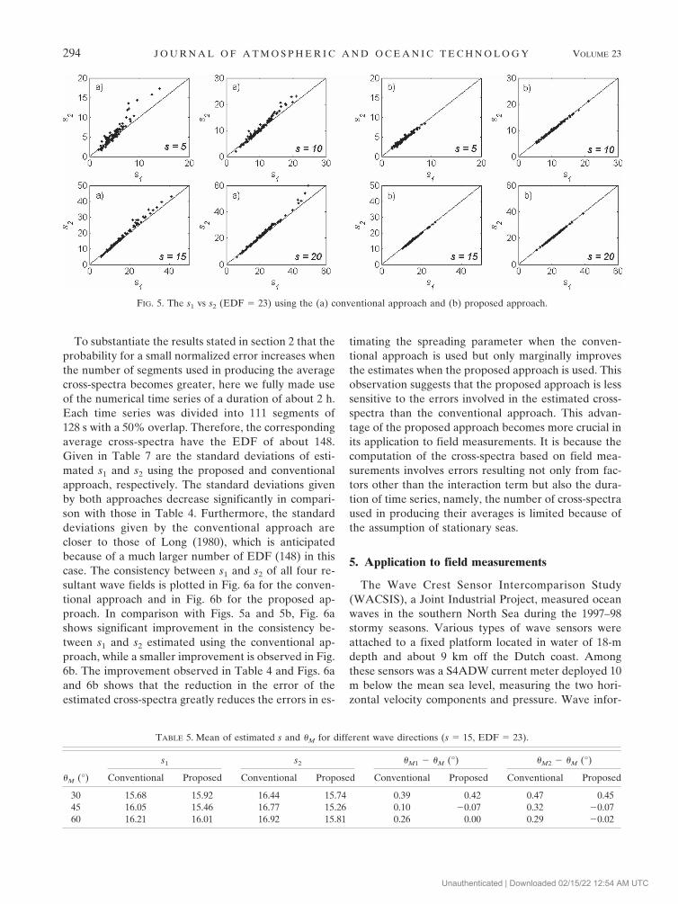
To substantiate the results stated in section 2 that theprobability for a small normalized error increases whenthe number of segments used in producing the averagecross-spectra becomes greater, here we fully made useof the numerical time series of a duration of about 2 h.Each time series was divided into 111 segments of128 s with a 50% overlap. Therefore, the correspondingaverage cross-spectra have the EDF of about 148.Given in Table 7 are the standard deviations of esti-mated s1 and s2 using the proposed and conventionalapproach, respectively. The standard deviations givenby both approaches decrease significantly in compari-son with those in Table 4. Furthermore, the standarddeviations given by the conventional approach arecloser to those of Long (1980), which is anticipatedbecause of a much larger number of EDF (148) in thiscase. The consistency between s1 and s2 of all four re-sultant wave fields is plotted in Fig. 6a for the conven-tional approach and in Fig. 6b for the proposed ap-proach. In comparison with Figs. 5a and 5b, Fig. 6ashows significant improvement in the consistency be-tween s1 and s2 estimated using the conventional ap-proach, while a smaller improvement is observed in Fig.6b. The improvement observed in Table 4 and Figs. 6aand 6b shows that the reduction in the error of theestimated cross-spectra greatly reduces the errors in es-

timating the spreading parameter when the conven-tional approach is used but only marginally improvesthe estimates when the proposed approach is used. Thisobservation suggests that the proposed approach is lesssensitive to the errors involved in the estimated cross-spectra than the conventional approach. This advan-tage of the proposed approach becomes more crucial inits application to field measurements. It is because thecomputation of the cross-spectra based on field mea-surements involves errors resulting not only from fac-tors other than the interaction term but also the dura-tion of time series, namely, the number of cross-spectraused in producing their averages is limited because ofthe assumption of stationary seas.

5. Application to field measurements

The Wave Crest Sensor Intercomparison Study(WACSIS), a Joint Industrial Project, measured oceanwaves in the southern North Sea during the 1997–98stormy seasons. Various types of wave sensors wereattached to a fixed platform located in water of 18-mdepth and about 9 km off the Dutch coast. Amongthese sensors was a S4ADW current meter deployed 10m below the mean sea level, measuring the two hori-zontal velocity components and pressure. Wave infor-

TABLE 5. Mean of estimated s and �M for different wave directions (s � 15, EDF � 23).

�M (°)

s1 s2 �M1 � �M (°) �M2 � �M (°)

Conventional Proposed Conventional Proposed Conventional Proposed Conventional Proposed

30 15.68 15.92 16.44 15.74 0.39 0.42 0.47 0.4545 16.05 15.46 16.77 15.26 0.10 �0.07 0.32 �0.0760 16.21 16.01 16.92 15.81 0.26 0.00 0.29 �0.02

FIG. 5. The s1 vs s2 (EDF � 23) using the (a) conventional approach and (b) proposed approach.



mation was also collected by a directional Waveriderbuoy measuring three components of wave-induced ac-celeration, which was moored about 1 km to the northof the platform. Comprehensive description of theWACSIS and its measurement are referred to in For-ristall et al. (2004). The measurements recorded by theS4ADW and Waverider are used here to examine theaccuracy and consistency of the two approaches in es-timating the directional spreading parameter and meanwave direction. Because second-order wave–wave in-teractions mainly affect wave characteristics in the fre-quency ranges that are relatively low or high with re-spect to the spectral peak frequency (Zhang et al.1996), to exclude the errors resulting from the neglectof second-order nonlinear wave–wave interactions inthis study we mainly focus our attention to the estimateof the directional spreading parameter and mean direc-tion of waves at the spectral peak frequency. It isknown that the spreading parameter at the spectralpeak reaches the maximum and decreases away fromthe peak frequency (Mitsuyasu et al. 1975; Hasselmannet al. 1980). To demonstrate the efficacy of the pro-posed approach not limited to the measurements at thespectral peaks, we also estimate the spreading param-eters at frequencies at the entire frequency domain us-ing both approaches. It should be noted that the esti-mate of the spreading parameters away from the spec-tral peak, especially at relatively high or lowfrequencies, can be further improved if the second-order bound waves are decoupled from the measure-ments, which will be conducted in our future study.

All available datasets recorded by the S4ADW andWaverider were screened based on the following threecriteria. First, if a dataset involves a lot of abnormal

spikes that were observed in some velocity recordsmade by the S4ADW, the related dataset was excludedin this study. Second, when the velocity component ofthe ocean currents in the mean wave direction is sig-nificant with respect to the wave phase velocity at thespectral peak frequency, the observed (or appearance)wave frequency can be significantly different from thecorresponding intrinsic frequency resulting from theDoppler effect, which may result in large errors in es-timating wave directional spreading unless the effect ofcurrent is properly accounted for (Zhang and Zhang2004). Hence, when the projected current velocity inthe mean wave direction is greater than 5% of thephase velocity at the spectral peak, the related datasetswere discarded. Third, the consistency between the es-timated �M1 and �M2 is excellent if the directionalspreading function of a wave field is of unimodal, asevidenced in our previous numerical tests. It is alsoknown that the estimated mean wave directions (�M1

and �M2) of a wave field of bi- or multimodal directionalspreading are significantly different. Therefore, signifi-cant differences between them can be viewed as a vitalsign of the sea states of bi- or multimode directionalspreading. Hence, if the difference between the �M1 and�M2 estimated using the conventional approach isgreater than 10°, the related wave field is thought to bebi- or multimodal and should not be modeled by a co-sine-2s spreading function. The related datasets wereconsequently rejected as well. It is noted that the casesthat were rejected because of the difference between�M1 and �M2 being greater than 10° are very few in theWACSIS datasets, accounting for about 3.4% of casesconsidered in our study.

After screening, we had 85 cases available to our

TABLE 6. Std dev of estimated s and �M for different wave directions (s � 15, EDF � 23).

�M (°)

s1 s2 �M1 (°) �M2 (°)

Conventional Proposed Conventional Proposed Conventional Proposed Conventional Proposed

30 6.64 3.81 7.87 3.83 4.38 3.41 5.18 3.5145 6.54 3.50 7.50 3.53 4.93 3.96 5.82 4.0460 6.66 3.90 7.81 3.94 4.64 3.41 5.47 3.53

TABLE 7. Std dev of the estimated s (�M � 0°, EDF � 148).

s

s1 s2

Long Conventional Proposed Long Conventional Proposed

5 0.68 0.73 0.53 0.94 0.96 0.5310 1.45 1.41 1.00 1.72 1.68 1.0015 2.30 2.58 1.54 2.60 2.88 1.5520 3.17 3.53 2.00 3.52 3.90 2.00



study, each of which was recorded by both S4ADW andWaverider. The related datasets were used as the inputto the two approaches for the estimate of the spreadingparameter and mean wave direction. The ratio of theprojecting current to the phase velocity and the signifi-cant wave height of 85 selected cases are summarized inFig. 7. Each dataset involves a 20-min time series of asampling rate at 2 Hz. Similar to our numerical tests, forobtaining the average cross-spectra each 20-min timeseries was divided into 17 segments of a 128-s durationwith a 50% overlap between two consecutive segments.

a. Datasets recorded by the directional Waveriderbuoy

Unlike a pitch–roll buoy measuring the vertical ac-celeration and two wave slopes in the x and y directions,

the directional Waverider buoy measures three accel-eration components (vertical, north, and west). Threemeasured acceleration components were then inte-grated twice in the time domain to render three corre-sponding components of the particle displacement,which were given in the WACSIS database. Consistentwith linear wave theory, we assumed that the threecomponents of the displacement were recorded at afixed point at the mean sea level. The first and secondFourier coefficients of the directional spreading func-tion of a measured wave field were calculated followingEq. (3) in using the conventional approach.

The spreading parameters s1 and s2 and mean wavedirections �M1 and �M2 at the spectral peaks, estimatedusing the two approaches, respectively, are compared inFigs. 8 and 9. Similar to the trend observed in the re-

FIG. 6. The s1 vs s2 (EDF � 148) using the (a) conventional approach and (b) proposed approach.

FIG. 7. Histogram of (a) the ratio of the projecting current velocity in the mean wave direction to the phase velocity, and (b) thesignificant wave height.



lated numerical tests, the consistency between s1 and s2

estimated using the proposed approach is excellent,with virtually all points falling near the diagonal line asshown in Fig. 8b. On the other hand, Fig. 8a shows thatthe consistency of the conventional approach is poorand s2 is in general greater than s1. Almost all of theestimated s falls in the range from 5 to 20 in using theproposed approach. While most estimated s using theconventional approach falls in that range, in about 18%of the cases, s1 estimated using the conventional ap-proach is significantly greater than 20, which is toogreat and hence may be erroneous. The consistencybetween �M1 and �M2 is satisfactory as observed in bothFigs. 9a and 9b, although that given by the proposedapproach is slightly better. The satisfactory consistencymay partially result from the exclusion of the datasetsin which the difference between �M1 and �M2, estimated

using the conventional approach, is greater than 10°.Although the trends observed in these two figures arebased on the field measurements, they are very similarto those observed in the numerical tests.

b. Estimation based on the PUV

In applying the conventional approach, Eq. (3) wasused to compute the Fourier coefficients, except thatQ12 and Q13 are replaced by C12 and C13, respectively,where subscripts 1, 2, and 3 denote wave pressure, andthe x- and y-axis velocity components. The related re-sults are plotted in Figs. 10 and 11. As observed in Figs.10a and 10b, the consistency between s1 and s2 esti-mated using the proposed approach remains excellent,while that given by the conventional approach is ratherpoor. The estimated values of s2 are in general greater,and some are significantly greater than those of s1 in

FIG. 8. The s1 vs s2 estimated from Waverider data using the (a) conventional approach and (b) proposed approach.

FIG. 9. The �M1 vs �M2 estimated from Waverider data using the (a) conventional approach and (b) proposed approach.



using the conventional approach. The consistency be-tween estimated �M1 and �M2 is satisfactory. In short,the general trends observed in the cases of the PUVrecords are similar to those in the cases of the Wave-rider records. However, the consistency of either ap-proach is slightly deteriorated in comparison with thecorresponding one in the case of the Waveriderrecords.

c. Spreading parameters at frequencies away fromthe spectral peaks

To show that the proposed approach can also im-prove the estimate of the spreading parameters at fre-quencies other than the peak frequency, both ap-proaches were applied to the estimate of the spreadingparameters in the entire frequency domain for fourWaverider records. The four cases are named as

9803051100, 9803051120, 9803050500, and 9803050520.The names refer to the starting time for the relatedmeasurements (yy/mm/dd/hh/mm). The significantwave heights, peak frequencies, and ratios of windspeed to phase velocity at the peak frequency (U10/cp)of these cases are summarized in Table 8.

The dependence of the spreading parameter on thefrequency in all four cases is similar. For brevity, onlythe results of estimated s1 and s2 for case 9803051100are presented in Figs. 12a and 12b, respectively, depict-ing the estimated s1 and s2 using the conventional andproposed approaches as a function of the frequencynormalized by the peak frequency. For the purpose ofcomparison, also plotted in the figures is the empiricalcurve given by Hasselmann et al. (1980). It is observedthat s1 and s2 estimated by both approaches reach themaximum near the peak frequency and decrease when

FIG. 11. The �M1 vs �M2 estimated from PUV data using the (a) conventional approach and (b) proposed approach.

FIG. 10. The s1 vs s2 estimated from PUV data using the (a) conventional approach and (b) proposed approach.



the frequency moves away from the spectral peak. Theyare in satisfactory agreement with the trend of the em-pirical curves fitted based on the Joint North Sea WaveProgram (JONSWAP) data. It is also observed thatboth s1 and s2 fluctuate with respect to the empiricalcurves. Nevertheless, the fluctuation amplitude is muchsmaller in using the proposed approach.

To examine the consistency between estimated s1

and s2, we also compare the results of four cases in Fig.13a for the conventional approach and Fig. 13b for theproposed approach. The figures clearly show that theconsistency of s1 and s2 estimated using the proposedapproach is superior, similar to that observed in sec-tions 5a and 5b. In general, the estimated s2 is muchgreater than s1 in using the conventional approach. Theconsistency between s1 and s2 estimated using the pro-posed approach is excellent in the entire range of thespreading parameters, except for those of extremelysmall values (s � 2). The relatively large discrepanciesmainly occur at very low or high frequency rangeswhere nonlinear second-order (difference frequencyand sum frequency) bound waves are significant. It willbe our future effort to find out whether or not theconsistency can be improved after second-order boundwaves are filtered from the measurements.

6. Conclusions

The accuracy and consistency of the proposed andconventional approaches were examined in estimatingthe mean wave direction and spreading parameter atthe spectral peak of a wave field whose wave recordswere either numerically generated or measured in situ.In the case of the input being numerically generatedwave records, the comparison between the estimatesand the related prescribed values indicates that the pro-posed approach is statistically superior to the conven-tional approach, especially in estimating the directionalspreading parameter. Namely, the former renders analmost unbiased mean and significantly smaller stan-dard deviation in estimating the spreading parameter.When the field measurements were used as the input,the comparison between estimated s1 and s2 shows thatthe proposed approach results in substantially betterconsistency between them, which is consistent with thecorresponding observation made in the numerical tests.Furthermore, the spreading parameters of waves at fre-quencies other than the peak frequency were also esti-mated using both approaches and are qualitatively con-sistent with the trend given by Hasselmann et al. (1980).The consistency between s1 and s2 estimated using theproposed approach at the frequencies other than thepeak frequency is also found to be superior to thatusing the conventional approach. The consistency be-tween estimated s1 and s2 is especially crucial in ana-lyzing field measurements where the spreading param-eter of a measured wave field is not known.

The employment of a data adaptive method (MLM)to estimate the directional spreading function and thenits first two Fourier coefficients is the reason for the

FIG. 12. Dependence of s on f/fp for case 9803051100 (U10/cp � 1.35) using the (a) conventional approach and (b) proposedapproach.

TABLE 8. Sea states of selected four cases.

Case H1/3 (m) fp (Hz) U10/cp

9803050500 3.39 0.1240 1.399803050520 3.42 0.1289 1.519803051100 3.42 0.1143 1.359803051120 3.10 0.1143 1.34



superiority of the proposed approach over the conven-tional approach. This is because an MLM is more tol-erant of errors involved in the estimated cross-spectrathan is the DFT used in the conventional approach.Although the average of the cross-spectra may reduceerrors, especially those resulting from the “interaction”term, the reduction is limited by the duration of mea-sured wave records and the requirements of resolutionin the frequency domain. Hence, the use of the pro-posed approach in estimating the directional spreadingcoefficients of ocean wave is strongly recommended.Because a cosine-2s model is intended to model the seastates of unimode directional spreading and the efficacyof the proposed approach is only examined in these seastates in our study, it is not recommended to apply it tothe sea states of a bi- and multimode.

Acknowledgments. The authors gratefully acknowl-edge the partial financial support provided by the Off-shore Technology Research Center at Texas A&MUniversity.

REFERENCES

Earle, M. D., 1996: Nondirectional and directional wave dataanalysis procedures. DNBC Tech. Doc. 96-01, 37 pp.

Ewing, J. A., and A. K. Laing, 1987: Directional spectra of seasnear full development. J. Phys. Oceanogr., 17, 1696–1706.

Forristall, Z. G., and K. C. Ewans, 1998: Worldwide measure-ments of directional wave spreading. J. Atmos. Oceanic Tech-nol., 15, 440–469.

——, and Coauthors, 2004: Wave crest sensor intercomparisonstudy: An overview of WACSIS. J. Offshore Mech. Arct.Eng., 126, 26–34.

Harris, F. J., 1978: On the use of windows for harmonic analysiswith the discrete Fourier transform. Proc. IEEE, 66, 51–83.

Hashimoto, N., 1997: Analysis of the directional wave spectrafrom field data. Advances in Coastal and Ocean Engineering,Vol. 3, P.L.-F. Liu, Ed., World Scientific, 103–143.

Hasselmann, D. E., M. Dunckel, and J. A. Ewing, 1980: Direc-tional wave spectra observed during JONSWAP 1973. J.Phys. Oceanogr., 10, 1264–1280.

Hwang, P. A., and D. W. Wang, 2000: Airborne measurements ofthe wavenumber spectra of ocean surface waves. Part II: Di-rectional distribution. J. Phys. Oceanogr., 30, 2768–2787.

Isobe, M., K. Kondo, and K. Horikawa, 1984: Extension of MLMfor estimating directional wave spectrum. Proc. Symp. onDescription and Modeling of Directional Seas, Lyngby, Den-mark, Danish Hydraulic Institute, A-6-1–A-6-15.

Jefferys, E. R., 1987: Directional sea should be ergodic. Appl.Ocean Res., 9, 186–191.

Jenkins, G. M., and D. G. Watts, 1968: Spectra Analysis and ItsApplications. Holden Day, 525 pp.

Long, R. B., 1980: The statistical evaluation of directional spec-trum estimates derived from pitch/roll buoy data. J. Phys.Oceanogr., 10, 944–952.

Longuet-Higgins, M. S., D. E. Cartwright, and N. D. Smith, 1963:Observations of the directional spectrum of sea waves usingthe motions of a floating buoy. Ocean Wave Spectra, PrenticeHall, 111–132.

Massel, S. R., and R. M. Brinkman, 1998: On the determination ofdirectional wave spectra for practical applications. Appl.Ocean Res., 20, 357–374.

Miles, M. D., 1989: A note on directional random wave synthesisby the single summation method. Proc. 23d IAHR Congress,Vol. C, Ottawa, ON, Canada, IAHR, 243–250.

Mitsuyasu, H., F. Tasai, T. Suhara, S. Mizuno, M. Ohkusu, T.Honda, and K. Rikiishi, 1975: Observation of the directionalspectrum of ocean waves using a cloverleaf buoy. J. Phys.Oceanogr., 5, 750–760.

Sand, S. E., and A. E. Mynett, 1987: Directional wave generationand analysis. Proc. IAHR Seminar on Wave Analysis and

FIG. 13. Scatterplots of s1 and s2 estimated in the entire frequency domain using the (a) conventional approach and (b) proposedapproach.



Generation in Laboratory Basins, Lausanne, Switzerland,IAHR, 209–235.

Tucker, M. J., and E. G. Pitt, 2001: Waves in Ocean Engineering.Elsevier Science, 550 pp.

Wang, H. T., and C. B. Freise, 1997: Error analysis of the direc-tional wave spectra obtained by the NDBC 3-m pitch-rolldiscus buoy. IEEE J. Oceanic Eng., 22, 639–648.

Welch, P. D., 1967: The use of fast Fourier transform for the

estimation of power spectra: A method based on time aver-aging over short, modified periodgrams. IEEE Trans. AudioElectroacoust., AU-15, 70–73.

Zhang, J., L. Chen, M. Ye, and R. E. Randall, 1996: Hybrid wavemodel for unidirectional irregular waves. Part I. Theory andnumerical scheme. Appl. Ocean Res., 18, 77–92.

Zhang, S., and J. Zhang, 2004: Analysis of directional wave fieldswith strong current. Appl. Ocean Res., 26, 13–22.



Documents

A New Approach to Estimate Directional Spreading