A new approach to measuring competition in the loan markets of the

ISSN 1561081-0

9 7 7 1 5 6 1 0 8 1 0 0 5

WORKING PAPER SER IESNO 768 / JUNE 2007

A NEW APPROACH TO MEASURING COMPETITION IN THE LOAN MARKETS OF THE EURO AREA

by Michiel van Leuvensteijn, Jacob A. Bikker, Adrian A.R.J.M. van Rixtel

and Christoffer Kok Sørensen

In 2007 all ECB publications

feature a motif taken from the €20 banknote.

WORK ING PAPER SER IE SNO 768 / JUNE 2007

This paper can be downloaded without charge from http://www.ecb.int or from the Social Science Research Network

electronic library at http://ssrn.com/abstract_id=991604.

1 The authors are grateful to Francesco Drudi and participants of the Eurobanking Conference, Dubrovnik (May 2006), the XV International Tor Vergata Conference on ‘Money, Finance and Growth’, Rome (December 2006) and seminars at DNB, ECB and

BdE for valuable comments and suggestions. The views expressed in this paper are personal and do not necessarily reflect those of the ECB, CPB, DNB or BdE.

2 M. van Leuvensteijn was attached to the Directorate General Economics of the European Central Bank (ECB) when the paper was written. He is currently at the Netherlands Bureau for Economic Policy Analysis (CPB), P.O. Box 80510, 2508 GM,

The Hague, the Netherlands; e-mail: [email protected] J.A. Bikker is attached to De Nederlandsche Bank (DNB), Supervisory Policy Division, Strategy Department, P.O. Box 98,

NL-1000 AB Amsterdam, The Netherlands; e-mail: [email protected] When this paper was written, A. van Rixtel was affiliated with the ECB. He is currently at the International Economics and

International Relations Department, Banco de España (BdE), Alcalá 48, 28014 Madrid, Spain; e-mail: [email protected]

60066 Frankfurt am Main, Germany; e-mail: [email protected]

A NEW APPROACH TO MEASURING COMPETITION IN THE LOAN MARKETS OF

THE EURO AREA 1

by Michiel van Leuvensteijn 2, Jacob A. Bikker 3, Adrian A.R.J.M. van Rixtel 4

5 and Christoffer Kok Sørensen

5 C. Kok Sørensen is attached to the Directorate General Economics of the ECB, P.O. Box 160319,

© European Central Bank, 2007

AddressKaiserstrasse 2960311 Frankfurt am Main, Germany

Postal addressPostfach 16 03 1960066 Frankfurt am Main, Germany

Telephone +49 69 1344 0

Internethttp://www.ecb.int

Fax +49 69 1344 6000

Telex411 144 ecb d

All rights reserved.

Any reproduction, publication and reprint in the form of a different publication, whether printed or produced electronically, in whole or in part, is permitted only with the explicit written authorisation of the ECB or the author(s).

The views expressed in this paper do not necessarily reflect those of the European Central Bank.

The statement of purpose for the ECB Working Paper Series is available from the ECB website, http://www.ecb.int.

ISSN 1561-0810 (print)ISSN 1725-2806 (online)

3ECB

Working Paper Series No 768June 2007

CONTENTS

Abstract 4

Non-technical summary 5

1 Introduction 7

2 Literature on measuring competition 8

3 The Boone indicator model 9

14

5 Estimation results 16 5.1 Marginal costs 16 17 5.2.1 Degree of competition across countries 18 5.2.2 Developments in competition over the years 21 5.2.3 Competition in the separate bank categories 25

6 Conclusions 29

References 30

European Central Bank Working Paper Series 34

5.2 The Boone indicator

Appendix: Estimations of the translog cost function 32

4 The data

Abstract This paper is the first that applies a new measure of competition, the Boone indicator, to the

banking industry. This approach is able to measure competition of bank market segments, such as

the loan market, whereas many well-known measures of competition can consider the entire

banking market only. A caveat of the Boone-indicator may be that it assumes that banks generally

pass on at least part of their efficiency gains to their clients. Like most other model-based

measures, this approach ignores differences in bank product quality and design, as well as the

attractiveness of innovations. We measure competition on the lending markets in the five major

EU countries as well as, for comparison, the UK, the US and Japan. Bearing the mentioned

caveats in mind, our findings indicate that over the period 1994-2004 the US had the most

competitive loan market, whereas overall loan markets in Germany and Spain were among the

best competitive in the EU. The Netherlands occupied a more intermediate position, whereas in

Italy competition declined significantly over time. The French, Japanese and UK loan markets

were generally less competitive. Turning to competition among specific types of banks,

commercial banks tend to be more competitive, particularly in Germany and the US, than savings

and cooperative banks.

JEL code: D4, G21, L1;

Key words: Banking industry, competition, loan markets, marginal costs, market shares;

4ECB Working Paper Series No 768June 2007

NON-TECHNICAL SUMMARY

This paper investigates the measurement of competition in the EU banking sector. Bank

competition is pivotal to monetary policy as it may affect the way changes in the policy rates of

the European Central Bank (ECB) are passed on to the interest rates that banks offer their

customers.

The paper uses a new approach, the so-called Boone indicator, to estimate competition in

the loan markets of the euro area. To our knowledge, this is the first paper which applies this

method to the banking market. This indicator measures the effect of efficiency on performance in

terms of profits or market shares. The idea underlining the Boone indicator is that competition

enhances the performance of efficient firms and impairs the performance of inefficient firms,

which is reflected in lower profits or smaller market shares.

Our approach is innovative in the sense that this method allows measurement of

competition not only for the entire banking market, but also for separate product markets, such as

the loan market, and for single types of banks, such as commercial, savings and cooperative

banks. By contrast, other often applied measures of bank competition, such as the Panzar-Rosse

model, typically only investigate the competitive nature of the aggregate of all banking activities.

Another advantage of the Boone indicator is that it requires relatively little data, contrary to many

other approaches, e.g. the Bresnahan model, which are very data intensive. That serves for the

estimation of competition on an annual basis, which enables us to assess developments in

competitive conditions over time. A disadvantage of the Boone-indicator is that it assumes that

banks generally pass on at least part of their efficiency gains to their clients. Furthermore, like

many other model-based measures, our approach ignores differences in product quality and

design across banks, as well as the attractiveness of innovations.

We apply the Boone indicator to the loan markets of the five major countries in the euro

area and, for comparison, to the UK, the US and Japan over 1994–2004. Our findings indicate

that the US had the most competitive loan market, whereas Germany and Spain were among the

best competitive EU markets. The German results seem to be driven partly by a competitive

commercial banking sector reflecting the distinct nature of its “three-pillar” banking system. In

Spain, competition remained strong and relatively stable over the full sample period, indicating

the progress the Spanish banking system has made since the major liberalisation reforms in the

late 1980s and early 1990s. The Netherlands took up a more intermediate position among the

countries in our sample, despite having a relatively concentrated banking market dominated by a

small number of very large players. Italian competition declined significantly over time, which

may be due to the partial reconstitution of market power by the banking groups formed in the

early 1990s. French and British loan markets were less competitive overall. In Japan, competition

in loan markets was found to increase dramatically over the years, in line with the consolidation

and revitalisation of the Japanese banking industry in recent years.

5ECB


The paper also measures competition among specific types of banks. Commercial banks,

which are more exposed to competition from foreign banks and capital markets, tend to be more

competitive, particularly in Germany and the US, than savings and cooperative banks, which

typically operate in local markets. An exception is Japan, where competition among savings and

cooperative banks was considerably stronger than competition between commercial banks. This

may indicate the adverse impact of the banking crises on bank competition, as the commercial

banks were particularly hard-hit by the severe banking crisis that engulfed Japan during the

1990s.

All in all, according to the Boone indicator, competitive conditions in the loan markets

and their developments over time are found to differ considerably across countries. These

differences seem largely to reflect distinct characteristics of the national banking sectors, such as

the relative importance of commercial, cooperative and saving banks respectively, and changes to

the banks’ institutional and regulatory environment during our sample period.


1. Introduction This paper investigates the measurement of competition in the EU banking sector. Competition is

a key driver of social welfare, as it may push down prices (i.e. interest rates) and improves

services for consumers and enterprises (Cetorelli, 2001).1 Also, competition is pivotal to

monetary policy: in a competitive market, changes in the policy rates of the European Central

Bank (ECB) are passed on more quickly to the interest rates that banks offer their customers.

The paper presents estimates of competition in loan markets of the major EU countries

using a new approach, introduced and applied by Boone (2000, 2004), Boone et al. (2004) and

CPB (2000). So far this method has not been applied to banking markets.2 The so-called Boone

indicator measures the impact of efficiency on performance in terms of profits or market shares.

The idea behind the Boone indicator is that competition enhances the performance of efficient

firms and impairs the performance of inefficient firms, which is reflected in their respective

profits or market shares. This approach is related to the well-known efficiency hypothesis, which

also explains banks’ performances by differences in efficiency (Goldberg and Rai, 1996;

Smirlock, 1985).

A well-known problem in the banking industry is that competition cannot be measured

directly, as costs and often also price data of single banking products are usually unavailable.

Hence, indirect measures are needed. This paper adds to the competition literature in applying a

new competition indicator to the banking sector which is an improvement on widely accepted

concentration measures, such as the Herfindahl-Hirschmann Index (HHI). The HHI has the

disadvantage of not distinguishing between large and small countries. Furthermore, concentration

may also be due to consolidation forced by severe competition. Hence, the concentration index is

an ambiguous measure.3

Our approach to competition is also innovative in the sense that we can measure

competition not only for the entire banking market, but also for various product markets, such as

the loan market, and for several types of banks, such as commercial, savings banks and

cooperative banks. An often applied measure such as the Panzar-Rosse model only investigates

the competitive nature of the total of all banking activities. Another advantage of the Boone

indicator is that it requires relatively little data, different from, e.g. the Bresnahan model which is

very data intensive. This allows the estimation of competition on an annual basis to assess

developments over time. A disadvantage of the Boone-indicator is that it assumes that banks

generally pass on at least part of their efficiency gains to their clients. Like many other model-

1 However, as is stressed by Allen et al. (2001), there is a conflict between this traditional view, stemming from the industrial organisation literature, and more recent theoretical models of bank competition, which raise the question whether competition between banks is good or bad. See, for example, Cetorelli and Strahan (2006). 2 Boone has applied his indicator to various manufacturing industries and Bikker and Van Leuvensteijn (2007) to the life insurance business. 3 A world-wide study by Claessens and Laeven (2004) found that bank concentration was positively instead of negatively related to competition.

7ECB


based measures, our approach ignores differences in bank product quality and design, as well as

the attractiveness of innovations.

The structure of this paper is as follows. Section 2 presents an overview of different

approaches in the literature to measure banking competition. Section 3 provides a theoretical

basis for the Boone indicator as a new measure for competition and discusses its properties. The

data are described in the following section. The econometric method and the results are presented

in Section 5. Finally, Section 6 concludes.

2. Literature on measuring competition

Competition in the banking sector has been analysed by measuring market power and efficiency.

A well-known approach to measuring market power is suggested by Bresnahan (1982) and Lau

(1982), recently used by Bikker (2003) and Uchida and Tsutsui (2005). They analyse bank

behaviour on an aggregate level and estimate the average conjectural variation of banks. A high

conjectural variation implies that a bank is highly aware of its interdependence with other firms in

terms of output and prices (via the demand equation). Under perfect competition where output

price equals marginal costs, the conjectural variation between banks should be zero, whereas a

value of one would indicate monopoly.

Panzar and Rosse (1987) propose an approach based on the so-called H-statistic which is

the sum of the elasticities of the reduced-form revenues with respect to the input prices. This H-

statistic ranges from -∞ to 1. An H-value equal to or smaller than zero indicates monopoly or

perfect collusion, whereas a value between zero and one provides evidence of a range of

oligopolistic or monopolistic types of competition. A value of one points to perfect competition.

This approach has been applied to all EU countries by Bikker and Haaf (2002).

A third indicator for market power is the Hirschman-Herfindahl Index, which measures

the degree of market concentration. This indicator is often used in the context of the ‘Structure

Conduct Performance’ (SCP) model (see e.g. Berger et al., 2004, and Bos, 2004), which assumes

that market structure affects banks’ behaviour, which in turn determines their performance.4 The

idea is that banks with larger market shares may have more market power and use that. Moreover,

a smaller number of banks make collusion more likely. To test the SCP-hypothesis, performance

(profit) is explained by market structure (as measured by the HHI).

Market power may also be related to profit, in the sense that extremely high profits may

be indicative of a lack of competition. A traditional measure of profitability is the price-cost

margin (PCM), which is equal to the output price minus the marginal costs, divided by the output

price. The PCM is frequently used in the empirical industrial organization literature as an

empirical approximation of the theoretical Lerner index.5 In the literature, banks’ efficiency is

4 Bikker and Bos (2005), pages 22 and 23. 5 The Lerner index derives from the monopolist's profit maximisation condition as price minus marginal cost, divided by price. The monopolist maximises profits when the Lerner index is equal to the inverse


often seen as a proxy of competition. The existence of scale and scope economies has in the past

been investigated thoroughly. It is often assumed that unused scale economies would be exploited

and, consequently, reduced under strong competition.6 Hence, the existence of non-exhausted

scale economies is an indication that the potential to reduce costs has not been exhausted and,

therefore, can be seen as an indirect indicator of (a lack of) competition (Bikker and Van

Leuvensteijn, 2007). The existence of scale efficiency is also important as regards the potential

entry of new firms, which is a major determinant of competition. Strong scale effects would put

new firms into an unfavourable position.

A whole strand of literature is focused on X-efficiency, which reflects managerial ability

to drive down production costs, controlled for output volumes and input price levels. The X-

efficiency of firm i is defined as the difference in costs between that firm and the best practice

firms of similar size and input prices (Leibenstein, 1966). Heavy competition is expected to force

banks to drive down their X-inefficiency, so that the latter is often used as an indirect measure of

competition. An overview of the empirical literature is presented in Bikker (2004) and Bikker and

Bos (2005).

A final area in the literature has been devoted to the Structure Conduct Performance

(SCP) model where conduct reflects competitive behaviour. This hypothesis assumes that market

structure affects competitive behaviour and, hence, performance. Many articles test this model

jointly with an alternative explanation of performance, namely the efficiency hypothesis, which

attributes differences in performance (or profit) to differences in efficiency (e.g. Goldberg and

Rai, 1996, and Smirlock, 1985). As mentioned above, the Boone indicator can be seen as an

elaboration on this efficiency hypothesis. This test is based on estimating an equation which

explains profits by market structure variables and measures of efficiency. The efficiency

hypothesis assumes that market structure variables do not contribute to profits once efficiency is

considered as cause of profit. As Bikker and Bos (2005) show, this test suffers from a

multicollinearity problem if the efficiency hypothesis holds.

3. The Boone indicator model

Boone’s model is based on the notion, first, that more efficient firms (that is, firms with lower

marginal costs) gain higher market shares or profits and, second, that this effect is stronger the

heavier the competition in that market is. In order to support this quite intuitive market

characteristic, Boone develops a broad set of theoretical models (see Boone, 2000, 2001 and

2004, Boone et al., 2004, and CPB, 2000). We use one of these models to explain the Boone

price elasticity of market demand. Under perfect competition, the Lerner index is zero (market demand is infinitely elastic), in monopoly it approaches one for positive non-zero marginal cost. The Lerner index can be derived for intermediary cases as well. For a discussion see Church and Ware (2000). 6 This interpretation would be different in a market numbering only a few firms. Furthermore, this interpretation would also change when many new entries incur unfavourable scale effects during the initial phase of their growth path.

9ECB


indicator and to examine its properties compared to common measures such as the HHI and PCM

approaches. Following Boone et al. (2004), and replacing ‘firms’ by ‘banks’, we consider a

banking industry where each bank i produces one product qi (or portfolio of banking products),

which faces a demand curve of the form:

p (qi, qj≠i) = a – b qi – d ∑j≠i qj (1)

and has constant marginal costs mci. This bank maximizes profits πi = (pi – mci) qi by choosing the

optimal output level qi. We assume that a > mci and 0 < d ≤ b. The first-order condition for a

Cournot-Nash equilibrium can then be written as:

a –2 b qi – d ∑ i≠j qj – mci = 0 (2)

When N banks produce positive output levels, we can solve the N first-order conditions (2),

yielding:

qi (ci) = [(2 b/d – 1) a – (2 b/d + N – 1) mci + ∑ j mcj]/[(2 b + d (N – 1))(2 b/d – 1)] (3)

We define profits πi as variable profits excluding entry costs ε. Hence, a bank enters the banking

industry if, and only if, πi ≥ ε in equilibrium. Note that Equation (3) provides a relationship

between output and marginal costs. It follows from πi = (pi – mci) qi that profits depend on marginal

costs in a quadratic way.

In this market, competition can increase in two ways. First, competition increases when

the produced (portfolios of) services of the various banks become closer substitutes, that is, d

increases (keeping d below b). Second, competition increases when entry costs ε decline. Boone

et al. (2004) prove that market shares of more efficient banks (that is, with lower marginal costs

c) increase both under regimes of stronger substitution and amid lower entry costs.

Equation (3) supports the use of the following model for market share, defined as si = qi / ∑ j qj:

ln si = α + β ln mci (4)

The market shares of banks with lower marginal costs are expected to increase, so that β is

negative. The stronger competition is, the stronger this effect will be, and the larger, in absolute

terms, this (negative) value of β. We refer to the β parameter as the Boone indicator. For

empirical reasons, Equation (4) has been specified in log-linear terms in order to deal with

heteroskedasticty. Moreover, this specification implies that β is an elasticity, which facilitates


easy interpretation, particularly across equations.7 The choice of functional form is not essential,

as the log-linear form is just an approximation of the pure linear form. In Section 5.2.1, we will

find that the results of the linear model are very similar to those of the log-linear model.

The theoretical model above can also be used to explain why widely-applied measures

such as the HHI and the PCM fail as reliable competition indicators. The standard intuition of the

HHI is based on a Cournot model with symmetric banks, where a fall in entry barriers reduces the

HHI. However, with banks that differ in efficiency an increase in competition through a rise in d

reallocates output to the more efficient banks that already had higher output levels. Hence, the

increase in competition raises the HHI. The effect of increased competition on the industry’s

PCM may also be perverse. Generally, heavier competition reduces the PCM of all banks. But

since more efficient banks may have a higher PCM (skimming off part of the profits stemming

from their efficiency lead), the increase of their market share may raise the industry’s average

PCM, contrary to common expectations.

We note that the Boone indicator model, like every other model, is a simplification of

reality. First, efficient banks may choose to translate lower costs either into higher profits or into

lower output prices in order to gain market share. Our approach assumes that the behaviour of

banks is between these two extreme cases, so that banks generally pass on at least part of their

efficiency gains to their clients. More precisely, we assume that the banks’ passing-on behaviour,

which drives Equation (4), does not diverge too strongly across the banks. Second, our approach

ignores differences in bank product quality and design, as well as the attractiveness of

innovations. We assume that banks are forced over time to provide quality levels that are more or

less similar. By the same token, we presume that banks have to follow the innovations of their

peers. Hence, like many other model-based measures, the Boone indicator approach focuses on

one important relationship, affected by competition, thereby disregarding other aspects (see also

Bikker and Bos, 2005). Naturally, annual estimates of β are more likely to be impaired by these

distortions than the estimates covering the full sample period. Also, compared to direct measures

of competition, the Boone indicator may have the disadvantage of being an estimate and thus

surrounded by a degree of uncertainty. Of course, other model-based measures, such as Panzar

and Rosse’s H-statistic, suffer from the same disadvantage. The latter shortcoming concerns to

the annual estimates βt rather than the full sample period estimate β.

As the Boone indicator may be time dependent, reflecting changes in competition over

time, we estimate β separately for every year (hence, βt). We do not have an absolute benchmark

for the level of β. We only know that the more negative β is, the stronger competition must be.

Comparing the indicator across regions or countries, or even across industries, may help to

interpret estimation results. For that reason, Boone and Weigand in CPB (2000) and Boone et al.

(2004) applied the model to different manufacturing industries. Since measurement errors –

7 The few existing empirical studies based on the Boone indicator have all used a log linear relationship. See, for example, Bikker and Van Leuvensteijn (2007).

11ECB


including unobserved country or industry specific factors – are less likely to vary over time than

across industries, the time series interpretation of beta is probably more robust than the cross-

sector one (that is, comparison of β for various countries or industries at a specific moment in

time). Therefore, Boone focuses mainly on the change in βt over time within a given industry,

rather than comparing β between industries.

Because marginal costs cannot be observed directly, CPB (2000) and Boone et al. (2004)

approximate a firm’s marginal costs by the ratio of average variable costs and revenues. As

dependent variable in Equation (4), CPB (2000) uses the relative values of profits and as

explanatory variable the ratio of variable costs and revenues, whereas Boone et al. (2004)

consider absolute instead of relative values.

We improve on Boone’s approach in two ways. First, we calculate marginal costs instead

of approximating this variable with average variable costs. We are able to do so by using a

translog cost function, which is more precise and more closely in line with theory. An important

advantage is that these marginal costs allow focussing on segments of the market, such as the

loan market, where no direct observations of individual cost items are available. Second, we use

market share as dependent variable instead of profits. The latter is, by definition, the product of

market shares and profit margin. We have views on the impact of efficiency on market share and

its relation with competition, supported by the theoretical framework above, whereas we have no

a priori knowledge about the effect of efficiency on the profit margin. Hence, a market share

model will be more precise. An even greater advantage of using market shares is that they are

always positive, whereas the range of profits (or losses) includes negative values. A log linear

specification would exclude negative profits (losses) by definition, so that the estimation results

would be distorted by sample bias, because inefficient, loss-making banks would have to be

ignored.

In order to be able to calculate marginal costs, we first estimate, for each country, a

translog cost function (TCF) using individual bank observations. Such a function assumes that the

technology of an individual bank can be described by one multiproduct production function.

Under proper conditions, a dual cost function can be derived from such a production function,

using output levels and factor prices as arguments. A TCF is a second-order Taylor expansion

around the mean of a generic dual cost function with all variables appearing as logarithms. It is a

flexible functional form that has proven to be an effective tool in explaining multiproduct bank

services. The TCF has the following form:

ln cith = α0 + ∑h=1,..,(H-1) αh di

h + ∑t=1,..,(T-1) δt dt + ∑h=1,..,H ∑j=1,..,K βjh ln xijt dih

+∑h=1,..,H ∑j=1,..,K ∑k=1,..,K γjkh ln xijt ln xikt dih + vit (5)

where the dependent variable cith reflects the production costs of bank i (i = 1, .., N ) in year t (t =

1, .., T ). The sub-index h (h = 1, .., H ) refers to the type category of the bank, that is, commercial


bank, savings bank or cooperative bank. The variable dih is a dummy variable, which is 1 if bank i

is of type h and otherwise zero. The variable dt is a dummy variable, which is 1 in year t and

otherwise zero. The explanatory variables xikt represent three groups of variables (k = 1, .., K.).

The first group consists of (K1) bank output components, such as loans, securities and other

services (proxied by other income). The second group consists of (K2) input prices, such as wage

rates, deposit rates (as price of funding) and the price of other expenses (proxied as the ratio of

other expenses to fixed assets). The third group consists of (K-K1-K2) control variables (also

called ‘netputs’), e.g. the equity ratio. In line with Berger and Mester (1997), the equity ratio

corrects for differences in loan portfolio risk across banks. The coefficients αh, βjh and γjkh, all

vary with h, the bank type. The parameters δt are the coefficients of the time dummies and vit is

the error term.

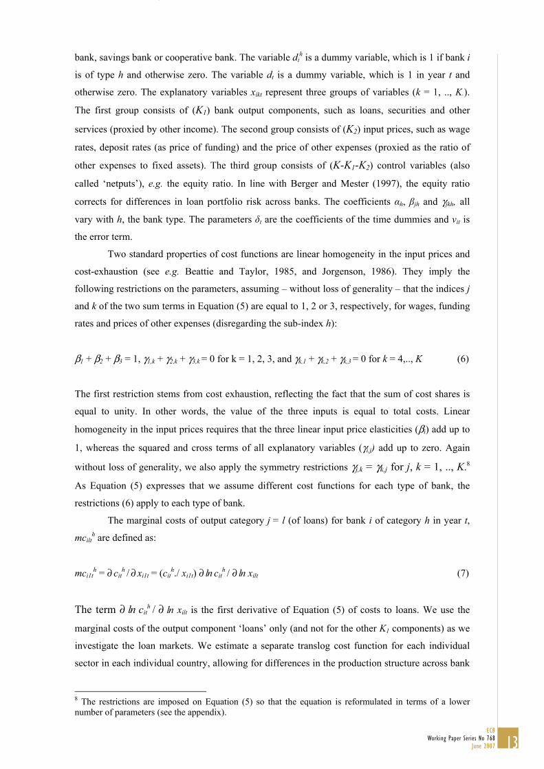
Two standard properties of cost functions are linear homogeneity in the input prices and

cost-exhaustion (see e.g. Beattie and Taylor, 1985, and Jorgenson, 1986). They imply the

following restrictions on the parameters, assuming – without loss of generality – that the indices j

and k of the two sum terms in Equation (5) are equal to 1, 2 or 3, respectively, for wages, funding

rates and prices of other expenses (disregarding the sub-index h):

β1 + β2 + β3 = 1, γ1,k + γ2,k + γ3,k = 0 for k = 1, 2, 3, and γk,1 + γk,2 + γk,3 = 0 for k = 4,.., K (6)

The first restriction stems from cost exhaustion, reflecting the fact that the sum of cost shares is

equal to unity. In other words, the value of the three inputs is equal to total costs. Linear

homogeneity in the input prices requires that the three linear input price elasticities (βi) add up to

1, whereas the squared and cross terms of all explanatory variables (γi,j) add up to zero. Again

without loss of generality, we also apply the symmetry restrictions γj,k = γk,j for j, k = 1, .., K.8

As Equation (5) expresses that we assume different cost functions for each type of bank, the

restrictions (6) apply to each type of bank.

The marginal costs of output category j = l (of loans) for bank i of category h in year t,

mcilth are defined as:

mci1th = ∂ cit

h / ∂ xi1t = (cith./ xi1t) ∂ ln cit

h / ∂ ln xilt (7)

The term ∂ ln cith / ∂ ln xilt is the first derivative of Equation (5) of costs to loans. We use the

marginal costs of the output component ‘loans’ only (and not for the other K1 components) as we

investigate the loan markets. We estimate a separate translog cost function for each individual

sector in each individual country, allowing for differences in the production structure across bank

8 The restrictions are imposed on Equation (5) so that the equation is reformulated in terms of a lower number of parameters (see the appendix).

13ECB


types within a country. This leads to the following equation of the marginal costs for output

category loans (l ) for bank i in category h during year t:

mci1th = cit

h / xi1t (β1h + 2 γ1lh ln xilt + ∑k=1,..,K; k ≠ l γ1kh ln xikt ) dih (8)

4. The data This paper uses an extended Bankscope database of banks’ balance sheet data running from 1992

to 2004. We investigate banking markets of the major euro area countries, i.e. France, Germany,

Italy, the Netherlands and Spain, as well as, for comparison, the UK, the US and Japan. The focus

is on commercial banks, savings banks, cooperative banks and mortgage banks and, for most

countries, ignores specialized banks, such as investment banks, securities firms and specialized

governmental credit institutions. For Germany, some specialized governmental credit institutions,

that is, the major Landesbanks, are included in the sample in order to have a more adequate

coverage of the German banking system. In addition to certain public finance duties, these

Landesbanks also offer banking activities in competition with the private sector banks

(Hackethal, 2004). For Japan, in contrast with Uchida and Tsutsui (2005), we also include three

long-term credit banks, because they traditionally have been offering long-term loans to the

corporate sector and have increasingly become competitors of the commercial banks, due to the

ongoing process of financial liberalisation in Japan which has eroded the traditional segmentation

of the Japanese banking sector (Van Rixtel, 2002).

In order to exclude irrelevant and unreliable observations, banks are incorporated in our

sample only if they fulfilled the following conditions: total assets, loans, deposits, equity and

other non-interest income should be positive; the deposits-to-assets ratio and loans-to-assets ratio

should be less than, respectively, 0.98 and 1; the income-to-assets ratio should be below 20

percent; personnel expenses-to-assets and other expenses-to-assets ratios should be between

0.05% and 5%; and finally, the equity-to-assets ratio should be between 1% and 50%. These

restrictions reduced the sample by 3,980 observations mainly due to the equity-to-assets ratio

restriction. As the Japanese banking sector experienced a deep crisis during most of our sample

period, we have relaxed the equity ratio restriction for Japanese banks.


Table 4.1. Number of banks by country and by type in 2002

Country Commercial banks

Cooperative banks

Long-term credit banks

Real estate banks/ Mortgage banks

Savings banks

Special governmental credit institutions Total

DE 130 867 0 44 501 28 1,570 ES 61 17 0 0 43 0 121 FR 115 83 0 2 30 0 230 UK 80 0 0 57 3 0 140 IT 105 476 0 1 52 0 634 JP 169 676 3 0 1 0 849 NL 24 1 0 4 1 0 30 US 7,921 1 0 1 914 0 8,837 Total 8,605 2,121 3 109 1,545 28 12,411

As a result, the data set for 2002 totals 8,605 commercial banks (including Landesbanks), 2,121

cooperative banks, 1,545 savings banks and 109 mortgage banks, plus 31 other banks, which are

12,411 banks in total (see Table 4.1). Over all years of the sample, the number of observations is

88,647. German and, particularly, US banks dominate the sample with, respectively, 1,570 and

8,837 banks (in 2002). Before 1999, the number of US banks is only around one quarter of this

number.

Table 4.2 gives a short description of the variables used in the estimations, such as costs,

loans, securities and other services, each expressed as a share of total assets, income or funding.

Costs are defined as the sum of interest expenses, personnel expenses and other non-interest

expenses. Costs, loans and securities are, respectively, 6%, 61% and 25% of total assets. Average

market shares differ strongly across countries, due mainly to country size effects. The output

factor other services is proxied by non-interest income, which is around 12% of total income.

Wage rates are proxied by personnel expenses as ratio of total assets, as for most banks the

number of staff is not available. Wages average 1.5% of total assets. The other-expenses-to-fixed-

assets ratio provides an input price for this input factor. Finally, interest rate costs, proxied by the

ratio of interest expenses and total funding, run to around 3.1%.

Table 4.2. Mean values of key variables by countries for the period 1992-2004 (in %)

Country

Total costs as a share of total assets

Average market share of lending

Loans as a share of total assets

Securities as a share of total assets

Other services as a share of total income

Other expenses as a share of fixed assets

Wages as a share of total assets

Interest expenses as a share of total funding

DE 6.44 0.06 60 22 12 227 1.5 3.7 ES 6.63 0.98 58 14 16 167 1.5 4.1 FR 7.42 0.41 54 4 20 537 1.5 4.8 UK 6.29 0.78 59 11 14 885 0.9 5.1 IT 6.67 0.22 53 26 16 261 1.7 3.5 JP 2.89 0.25 58 20 14 128 0.1 0.4 NL 6.59 0.54 54 15 13 340 0.9 5.4 US 5.63 0.01 63 28 11 148 1.6 2.8 Total 5.82 0.12 61 25 12 203 1.5 3.1

15ECB


5. Estimation results

5.1. Marginal costs

The first step of our estimation procedure is to calculate the marginal costs of the national

banking sectors, that is, we estimate Equation (8) for each of the respective eight countries. For

this purpose, we use the explanatory variables described in Section 4, namely bank outputs

(loans, securities and other services), input prices (wages, funding rates and prices of other non-

interest expenses) and the control variable (equity ratio). As an example, Table A.1 in the

appendix presents the translog cost function for Germany.9 The development of the marginal costs of loans for all individual countries during our

sample period is shown in Table 5.1. It is clear that these costs have gradually declined over time,

which to a large extent reflects the decrease in funding rates during 1992-2004. However, the

speed and magnitude of this decline differ across countries. Thus, differences in country specific

characteristics, such as banking technology or differences in legislation and supervision play a

role in the development of marginal costs. Germany and Spain have relatively high marginal

costs compared to the Netherlands, which may be related to population density. A low population

density may raise operating costs in relative terms, because it makes the retail distribution of

banking services relatively more costly. Table 5.1 also shows that marginal costs in France are

the highest of all countries during the second half of our sample period.

Table 5.1. Marginal costs of loans over time, weighted by loans (in % of loans) 1)

Year/country DE ES FR UK IT JP NL US Average 1992 10.2 15.9 13.8 14.5 13.2 6.0 9.2 – 10.9 1993 9.4 17.2 13.4 11.3 12.0 5.4 8.1 – 9.8 1994 9.2 14.3 11.9 9.8 12.2 5.4 7.4 – 9.1 1995 8.9 15.4 11.7 10.2 11.8 5.6 7.1 – 9.3 1996 8.5 14.3 10.9 9.2 11.3 4.5 6.3 – 8.8 1997 7.4 11.7 10.9 9.0 9.7 5.0 6.4 – 8.2 1998 7.1 11.1 11.2 10.3 7.5 5.1 7.4 – 7.9 1999 6.4 8.8 10.0 7.7 6.7 4.0 6.4 6.8 6.8 2000 7.1 9.9 11.2 8.0 6.7 3.0 6.5 7.4 7.3 2001 7.3 9.6 11.7 7.2 6.6 3.2 6.4 6.9 7.6 2002 7.1 7.8 10.7 6.3 6.1 3.1 5.7 5.6 6.7 2003 6.4 5.9 8.9 5.8 5.3 2.8 4.9 4.9 5.9 2004 6.0 4.8 7.9 5.6 4.9 2.7 4.6 4.5 5.4

1) Marginal costs are first calculated with Equation (8) at the individual bank level. Next, the numbers are weighted by the amount of loans on the balance sheet and aggregated by country and by year.

Table 5.2 shows that commercial banks in general have higher marginal costs than savings and

cooperative banks. A possible explanation is that these banks attract fewer deposits and therefore

have higher funding costs.

9 The translog cost functions for the other countries may be obtained from the authors.


Table 5.2. Marginal costs by country and by bank type in 2002 (in % of loans) 1)

Country Commercial banks Savings banks Cooperative banks DE 7.14 5.80 6.13 ES 10.12 4.67 4.96 FR 10.31 6.89 11.52 UK 4.94 9.63 – IT 6.64 4.28 4.77 JP 1.95 0.56 3.15 NL 6.52 – 3.83 US 5.71 4.78 –

1) Marginal costs are first calculated with Equation (8) at the individual bank level. Next, the numbers are weighted by the amount of loans on the balance sheet and aggregated by country, by year and by bank type.

5.2. The Boone indicator

Given the estimated marginal costs from the previous section, we are now able to estimate the

Boone indicator. To do so, we use for each country the relationship between the marginal costs of

individual banks and their market shares as in Equation (4): 10

ln silt = α + β ln mcilt + ∑t=1,..,(T-1) γt dt + uilt (9)

where s stands for market share, mc for marginal costs, i refers to bank i, l to output type ‘loans’,

and t to year t; dt. are time dummies (as in Equation (5)) and uilt is the error term. This provides us

with the coefficient β, the Boone indicator. We estimate this equation for, respectively, the overall

banking sector in each country (Sections 5.2.1 and 5.2.2) and for the various banking categories

separately: commercial banks, savings banks, cooperative banks and mortgage banks (Section

5.2.3). We present country estimates of β both for the entire period, referred to as full sample

period estimates, and for each year separately, referred to as annual estimates.

The estimations are carried out using the Generalized Method of Moments (GMM) with

as instrument variables the one-, two- or three-year lagged values of the explanatory variable,

marginal costs.11 To test for overidentification of the instruments, we apply the Hansen J-test for

GMM (Hayashi, 2000). The joint null hypothesis is that the instruments are valid instruments, i.e.

uncorrelated with the error term. Under the null hypothesis, the test statistic is chi-squared with

the number of degrees of freedom equal to the number of overidentification restrictions. A

rejection would cast doubt on the validity of the instruments. Further, the Anderson canonical

correlation likelihood ratio is used to test for the relevance of excluded instrument variables

(Hayashi, 2000). The null hypothesis of this test is that the matrix of reduced form coefficients

has rank K-1, where K is the number of regressors, meaning that the equation is underidentified.

Under the null hypothesis of underidentification, the statistic is chi-squared distributed with L-

K+1 degrees of freedom, where L is the number of instruments (whether included in the equation

10 As bank types do not play any role here, we do not refer to the index h. (Compare to Equation (11)). 11 For Germany, the one-, two- or three-year lagged values of the average costs are used.

17ECB


or excluded). This statistic provides a measure of instrument relevance, and rejection of the null

hypothesis indicates that the model is identified. We use kernel-based heteroskedastic and

autocorrelation consistent (HAC) variance estimations. The bandwidth in the estimation is set at

two periods and the Newey-West kernel is applied. Where the instruments are overidentified,

2SLS is used instead of GMM. For this 2SLS estimator, Sargan's statistic is used instead of the

Hansen J-test.

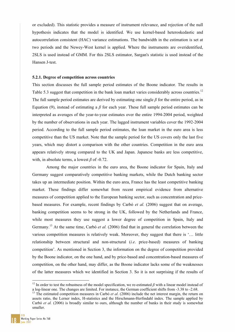
5.2.1. Degree of competition across countries

This section discusses the full sample period estimates of the Boone indicator. The results in

Table 5.3 suggest that competition in the bank loan market varies considerably across countries.12

The full sample period estimates are derived by estimating one single β for the entire period, as in

Equation (9), instead of estimating a β for each year. These full sample period estimates can be

interpreted as averages of the year-to-year estimates over the entire 1994-2004 period, weighted

by the number of observations in each year. The lagged instrument variables cover the 1992-2004

period. According to the full sample period estimates, the loan market in the euro area is less

competitive than the US market. Note that the sample period for the US covers only the last five

years, which may distort a comparison with the other countries. Competition in the euro area

appears relatively strong compared to the UK and Japan. Japanese banks are less competitive,

with, in absolute terms, a lowest β of -0.72.

Among the major countries in the euro area, the Boone indicator for Spain, Italy and

Germany suggest comparatively competitive banking markets, while the Dutch banking sector

takes up an intermediate position. Within the euro area, France has the least competitive banking

market. These findings differ somewhat from recent empirical evidence from alternative

measures of competition applied to the European banking sector, such as concentration and price-

based measures. For example, recent findings by Carbó et al. (2006) suggest that on average,

banking competition seems to be strong in the UK, followed by the Netherlands and France,

while most measures they use suggest a lower degree of competition in Spain, Italy and

Germany.13 At the same time, Carbó et al. (2006) find that in general the correlation between the

various competition measures is relatively weak. Moreover, they suggest that there is ‘… little

relationship between structural and non-structural (i.e. price-based) measures of banking

competition’. As mentioned in Section 3, the information on the degree of competition provided

by the Boone indicator, on the one hand, and by price-based and concentration-based measures of

competition, on the other hand, may differ, as the Boone indicator lacks some of the weaknesses

of the latter measures which we identified in Section 3. So it is not surprising if the results of

12 In order to test the robustness of the model specification, we re-estimated β with a linear model instead of a log-linear one. The changes are limited. For instance, the German coefficient shifts from -3.38 to -2.68. 13 The estimated competition measures in Carbó et al. (2006) include the net interest margin, the return on assets ratio, the Lerner index, H-statistics and the Hirschmann-Herfindahl index. The sample applied by Carbó et al. (2006) is broadly similar to ours, although the number of banks in their study is somewhat smaller.


Carbó et al. (2006) differ from ours. We compare our estimates of the full-sample period Boone

indicator with the HHI statistic and find a Pearson correlation coefficient of 0.30. This suggests

that a higher number of banks (or lower concentration) correlates positively, be it weakly, with a

larger (negative) value, in absolute terms, of the Boone indicator (indicating stronger

competition).

Contrary to recent criticism on the functioning of the German banking sector (e.g. IMF,

2004), our estimates suggest that this sector is among the most competitive in the euro area. Most

likely, this result for Germany hinges in part on the special structure of its banking system, being

built on three pillars, namely commercial banks, publicly-owned savings banks and cooperative

banks (see Hackethal, 2004). Contrary to most other euro area countries, the total market share of

the commercial banks in the loan and deposit markets is relatively limited, amounting to a mere

20-30%. Thus, this distinct characteristic of the German banking system may partly explain why

competition is found to be strongest in this country, since the Boone indicator is based on the

relationship between banks’ relative marginal costs (which in Germany, as in most countries,

were found to be lower for the non-commercial banks than for the commercial banks) and their

market share (which is larger for the non-commercial banks in Germany than for those in other

countries). Hence, our results should not be seen as contradicting the concerns of the IMF (see

IMF, 2004) about the inflexibility and distortive effects of the so-called three-pillar system in

Germany, but rather as reflecting the structural characteristics discussed above (see also Section

5.2.3). The Boone indicator for Germany may rather reflect the competitive environment of the

commercial banking sector, which operates countrywide, than the competitiveness of the savings

and cooperative banks that, generally, are active in regional markets only.

Table 5.3. Estimates of the Boone indicator over 1994-2004 for various countries

1) Asterisks indicate 95% (*) and 99% (**) levels of confidence. 2) The z-value indicates whether the parameter significantly differs from 0 under the normal distribution with zero mean and standard deviation one. 3) For Germany and the US, 2SLS is used and the equation is exactly identified, so that the Hansen J-test statistic is 0.00.

Boone indicator1) z-value2) F-test

Anderson canon. corr. LR-test

Hansen J-test (p-value)

Number of observations

DE3) **-3.38 -10.80 18.03 930.7 0.00 14,534 ES **-4.15 -3.99 2.87 162.7 1.339 (0.25) 734 FR **-0.90 -4.89 7.98 1,122.7 1.816 (0.18) 936 IT **-3.71 -7.77 19.16 1,613.6 1.690 (0.19) 3,419 NL **-1.56 -3.46 2.59 159.2 1.106 (0.29) 197 UK **-1.05 -3.12 1.50 1,068.4 0.396 (0.52) 787 US3) **-5.41 -40.49 345.04 9,916.0 0.00 40,177 JP *-0.72 -2.26 14.08 402.1 4.88 (0.03) 1,423

19ECB


The results for Spain and Italy seem to be driven mainly by the boost to competition following

the deregulation and liberalisation of the banking sector in the two countries in the early 1990s.14

In the Netherlands, the banking sector went through a process of profound reorganisation and

consolidation during the 1980s and 1990s.15 This development increased concentration in the

Dutch banking sector, but may also have led to efficiency improvements. All in all, the Boone

indicator suggests that from an international perspective competitive conditions in the Dutch

banking sector take up an intermediate position.16 Finally, the French banking sector is found to

be the least competitive of the euro area countries considered. This finding may in part stem from

the fact that although most French banks have now been privatized and the government continues

its withdrawal from the banking industry, the role of the State in the French banking sector

remains non-negligible, in that some important entities remain State-controlled (see for example:

Fitch Ratings, 2001; Moody’s Investors Service, 2004; S&P, 2005b).

Turning to the non-euro area countries, the Boone indicator suggests that in the UK,

competition in the loan market is weak. This may be because in specific segments of the UK loan

market, in particular mortgage lending, other institutions play an important role.17 Our results are

in line with Drake and Simper (2003) who find that due to the change in the ownership structure

of building societies (‘de-mutualisation’) competition in retail banking activities in the UK

declined during 1999-2001. As a matter of fact, the Boone indicator for the loan market without

the real estate and mortgage banks shows that competition in this segment is significantly

stronger.18

The US banking sector appears to be the most competitive among the countries in our

sample, reflecting the significant changes in the US banking system over the past two decades.

While it remains largely bifurcated along metropolitan and rural lines and continues to hinge on

the principles of specialisation and regionalism (basically stemming from legislation enacted

following the Great Depression), especially the lifting of restrictions on the range of banking

activities and of the ban on interstate banking have transformed the US banking system.19

14 See for example S&P (2004) and Moody’s Investors Service (2006). Our results are in line with Maudos et al. (2002), who find that profit margins during that decade declined significantly in Spain, especially for commercial banks and, to a lesser extent, for saving banks. For Italy, Coccorese (2005) presents evidence for the largest eight Italian banks during 1988-2000 that despite increased concentration the degree of competition remained considerable. 15 See for example Moody’s Investors Service (2005a). 16 Our results are in line with other empirical investigations, such as on competition in the Dutch market for revolving consumer credit, which showed that this market is competitive indeed (see Toolsema, 2002). 17 The UK has over 100 mortgage lenders. See also Moody’s Investors Service (2005c). 18 According to Heffernan (2002), the mortgage market in the UK is relatively competitive, but in other market segments such as personal loans there is substantially less competition. Results for the UK of estimations using a sample in which the mortgage lenders can be obtained from the authors upon request. 19 See for overviews of the various legislative changes for example Cetorelli (2001), Clarke (2004) and Fitch Ratings (2005). Emmons and Schmid (2000) find evidence that even before most of this new legislation was enacted, banks and credit unions competed directly.


Finally, the poor result for Japan is largely driven by the regulation of the banking

industry during the 1990s. As will be shown in the next section, however, competition in the

Japanese loan market increased dramatically during the period under investigation.

This section’s estimates, based on the entire sample period, may conceal considerable

differences over time and across types of banks. We investigate developments in the level of

competition over time in the next section and differences across types of banks in Section 5.2.3.

5.2.2. Developments in competition over the years

Table 5.4 shows the estimates of the Boone indicator across countries and over time (usually

1994-2004, depending on the respective country), based on:

ln silt = α + ∑t=1,..,T βt dt ln mcilt + ∑t=1,..,(T-1) γt dt + uilt (10)

Note that, in this section, the indicator βt is time dependent. While the above conclusions based

on the full sample period estimates generally remain valid, there are some notable differences

across countries in the Boone indicator’s development during the sample period. In most

countries, not all the βt’s differ significantly from zero for all years. Only for the US, the betas

differ from zero for all years. For Spain and the Netherlands, we observe substantial jumps in the

series over time (see also Chart 5.1). However, generally, the estimated successive annual betas

do not differ significantly from each other.20 Finally, for Japan (for six years), France (for 2 years)

and the Netherlands and the UK (for one year), the value of βt is positive instead of, as expected,

negative, in line with the rationale of Equation (4).21 This paragraph discusses only the countries

with statistically significant changes over time: Italy, the US and Japan.22 Chart 5.1 shows the

results for the other countries.

The banking sector in Italy, particularly the savings banks, went through a process of

deregulation and liberalisation in the early 1990s, fuelled in part by the adoption of various EU

Directives on financial institutions, which led to a consolidation wave.23 Whereas the EU

legislative initiatives affected all EU banking sectors, their eventual impact on competition was

most probably driven by the actual implementation at the national level and by additional

country-specific initiatives. In Italy, in particular, these institutional and regulatory changes are

likely to have had a catalytic effect on competition, as our estimates suggest strong competition

20 In this paper, ‘significant’ refers to the 95% level of confidence all along. 21 An alternative explanation is that competition on quality may lead to both higher marginal costs and higher market shares. 22 For these countries a Wald test with an H0 hypothesis of no change over time was rejected at the 5% level of significance. 23 In the early 1990s, large universal banking groups were established in Italy, as various restrictions on business activities were abolished. See for example Fitch Ratings (2002b), Moody’s Investors Service (2005d) and S&P (2005a). The process of financial deregulation was partly affected via Community legislation such as the Second Banking Coordination Directive; see Angelini and Cetorelli (2003) and Cetorelli (2004). A largely similar development took place in Spain, where important mergers involving the largest commercial banks took place in 1999 and 2000. See, for example, Fitch Ratings (2002a).

21ECB


22

ECB Working Paper Series No 768June 2007

around the mid-1990s (see Coccorese, 2005; Gambacorta and Iannotti, 2005). In more recent

years, the new banking groups formed in the early 1990s may have been able to reconstitute some

market power, as our results point to a continuous decline in competition since 1997 (see also

Chart 5.2).24

Although our estimates of the Boone indicator for the US show a significantly increasing

trend (indicating a decline in competition),25 the level of competition remains comparatively high.

A possible explanation for this gradual decline of competition is the decrease in market share of

commercial banks, which are generally more competitive than savings banks, as will be shown in

Section 5.2.3 (see also Jones and Critchfield, 2005).

In Japan, competition seems to have improved significantly (see Chart 5.3). This

remarkable increase can be partly attributed to a history of no or very little competition in the mid-

1990s. The Wald test rejects the null hypothesis of no change at 1% for Japan. In particular, our

estimates show that the Japanese banking sector experienced a rather marked transformation from a

climate with very little competition in the mid-1990s to a more competitive environment in recent

years, to where Japan ranked second in 2004, behind the US. This partly reflects the process of

financial deregulation and the gradual resolution of the bad loan problems that plagued Japanese

banks throughout the 1990s (Van Rixtel, 2002). Eventually, this development involved the de-facto

nationalisation of the worst-performing institutions and a major wave of consolidations, resulting in

the establishment of a small number of large commercial banking groups in 2000 and 2001 (Van

Rixtel et al., 2004). Our estimates suggest that the profound and structural changes in the Japanese

banking sector have helped to foster a competitive environment.

Table 5.4. Developments of the Boone indicator over time for various countries2)

Germany1) France Italy1) The Boone indicator βt z-value βt z-value βt z-value 1993 -5.90 -1.18 1994 **-7.25 -3.24 1995 -4.47. -1.40 **-1.28 -3.36 **-4.51 -3.53 1996 **-7.09 -2.92 **-1.28 -3.56 **-5.58 -3.98 1997 **-4.64 -3.41 **-1.11 -3.55 **-5.89 -4.08 1998 **-5.10 -3.97 *-0.79. -1.99 **-4.60 -6.08 1999 **-2.60 -4.04 *-0.78 -2.30 **-4.05 -4.39 2000 **-2.50 -4.60 -0.46. -1.34 **-3.32 -4.39 2001 **-3.31 -7.02 -0.68. -1.67 **-2.66 -3.62 2002 **-4.53 -4.71 -0.40. -0.78 -1.59. -1.82 2003 **-2.73 -5.62 0.27. 0.39 **-2.42 -3.69 2004 **-2.66 -4.15 0.10. 0.12 **-1.81 -2.79 F-test 10.70 5.10 13.23 Anderson canon corr. LR-test 185.2 1,023.7 300.3 Hansen J-test 0.00 19.69 (0.48) 0.00 Number of observations 14,534 918 4,918

24 In 2005 and 2006, a new wave of consolidation in the Italian banking sector was initiated. However, as our sample ends in 2004, our results do not capture these events. 25 The Wald test rejects the null hypothesis of no change at the 1% level of significance.

23

ECB Working Paper Series No 768

June 2007

Spain1) Netherlands US1) The Boone indicator βt z-value βt z-value βt z-value 1993 *-4.21 -2.49 1994 *-4.80 -2.28 -1.92 -1.42 1995 -5.20 -1.92 *-4.42 -2.42 1996 -9.61 -0.67 **-2.09 -2.58 1997 -4.36 -1.78 -3.57 -1.70 1998 -5.40 -0.86 1.04 0.38 1999 *-5.46 -2.21 -1.44 -0.85 2000 -3.44 -1.93 **-3.26 -3.00 **-6.89 -20.34 2001 **-4.38 -2.55 **-3.91 -4.71 **-6.16 -20.94 2002 *-3.88 -2.09 *-2.45 -2.44 **-5.54 -22.61 2003 -3.42 -1.20 -2.22 -1.80 **-4.87 -22.15 2004 **-2.69 -5.62 **-3.09 -2.85 **-4.54 -25.53 F-test 3.33 3.90 198.30 Anderson canon corr. LR-test 38.8 31.7 7,084.3 Hansen J-test 0.00 20.5 (0.04) 0.00 Number of observations 1,015 241 40,177

United Kingdom Japan The Boone indicator βt z-value βt z-value 1994 0.36 0.55 1995 -0.95 -1.57 **7.30 4.93 1996 -0.48 -0.64 **13.88 6.63 1997 -1.33 -1.52 **5.98 3.97 1998 *-1.87 -2.17 **3.97 4.04 1999 *-1.52 -1.96 **4.85 2.58 2000 *-1.56 -2.05 0.11 0.03 2001 *-1.46 -1.97 **-2.52 -4.04 2002 -1.22 -1.65 **-2.63 -3.73 2003 -0.43 -0.66 **-2.90 -6.56 2004 -0.49 -0.93 **-3.63 -5.95 F-test 1.25 23.48 Anderson canon corr. LR-test 1,468.2 214.8

Hansen J-test, (p-value) 20.88 (0.03) 34.43 (0.02) Number of observations 912 1476

Notes: Asterisks indicate 95% (*) and 99% (**) levels of confidence. Coefficients of time dummies have not been shown. 1) 2SLS is used and the equation is exactly identified, so that the Hansen J-test is 0.00. 2)

Equation (10) is estimated with the GMM. The number of observations for Italy, Japan, the Netherlands, Spain and the UK is higher than in Table 5.3, due to the use of instrumental variables with lags of a higher order in Table 5.3.

Chart 5.1. Indicators of the countries with no significant change in competition over time

-10

-8

-6

-4

-2

0

2

1993 1994 1995 1996 1997 1998 1999 2000 2001 2002 2003 2004

Boo

ne-in

dica

tor

The Netherlands Spain France UK Germany

Chart 5.2. Indicators of the countries with significantly diminishing competition over time

-8

-6

-4

-2

0

1993 1994 1995 1996 1997 1998 1999 2000 2001 2002 2003 2004

Boo

ne-in

dica

tor

Italy US


Chart 5.3. The indicator of the country with significantly improving competition over time

-5

0

5

10

15

1994 1995 1996 1997 1998 1999 2000 2001 2002 2003 2004

Boo

ne-in

dica

tor

Japan

5.2.3. Competition in the separate bank categories

Possibly, banks in some countries compete mainly with other banks in the same category, rather

than with all the other banks. It is conceivable that small cooperative and savings banks offer

mainly traditional bank products to retail customers and to small and medium-sized enterprises,

whereas the large commercial banks serve mainly larger firms and wealthy individuals in need of

a diversified palette of advanced services. In such countries, competition estimates for separate

bank categories may be more accurate than estimates based on all banks. Therefore, this section

estimates separate Boone indicators for commercial banks, savings banks and cooperative banks,

for all countries, except the Netherlands and the UK, based on:

ln silth = αh + ∑t=1,..,T βt

h ln mcilth + ∑t=1,..,(T-1) γt

h dth + uilt

h (11)

The banking sectors in the latter markets show only minor segmentation, so that estimating

indicators for specific bank categories seems irrelevant. For Germany we consider, on the one

hand, commercial banks and Landesbanks, which are assumed to compete with each other, and

on the other, cooperative banks and small savings banks, as they compete in local markets only

(see Hackethal, 2004). In Italy, competition is estimated separately for the three bank types

considered. Some cooperative banks, e.g. the banche populari, operate on a local level, whereas

the banche di credito cooperative (BCC) operate on a regional to national level, competing more

directly with the commercial banks (Fitch Ratings, 2002b). The sample of cooperative banks is

dominated by the BCCs, which also explains the fact that the level of competition is closely in

line with that of the Italian commercial banks. For the other countries, cooperative banks and

25ECB


savings banks are bundled together, as they behave quite similarly. The results are presented in

Table 5.5.

Particularly in Germany and the US, competition is found to be stronger among

commercial banks than among cooperative and savings banks. In Italy, commercial banks are

found to be more competitive than the savings banks for most of the period.26 These findings may

be explained by the fact that traditionally, savings banks and cooperative banks tend to operate at

the local level and have access to a stable and cheap pool of deposits from a loyal customer base.

Furthermore, savings and cooperative banks are often partly protected from competition, being

unable (either through regulation or by tradition) to compete across regional borders.27

Commercial banks are typically larger and operate on a national (or at least supra-regional) level,

where they face competition from other regional and foreign banks. Lacking easy access to a

stable pool of deposits, they depend more on costly interbank and market-based funding. They

provide loans and services predominantly to larger corporate customers and face competition

from the capital markets. These factors may induce commercial banks to behave more

competitively than the protected savings and cooperative banks.28

In France, the estimated degrees of competition among commercial banks and among

other banks are similar. This may be due to a considerable degree of consolidation across the

different banking sectors. Possibly, our results may be explained by this lack of effective or de

facto segmentation. However, the results for both the commercial banks and the other banks are

only significant for a limited number of years, and so should be interpreted carefully. In the case

of Spain, none of the yearly estimates for the category of savings and cooperative banks is

significant. As a matter of fact, it may be doubted whether segment specific estimation makes

sense for Spain, as savings banks, which dominate the other banks category, are seen to compete

at the national level with commercial banks, rather than at the regional or local level.29

Results for Japan indicate that the savings and cooperative banks there have generally

been more competitive than the commercial banks. This result may reflect the fact that savings

and cooperative banks were much less exposed to the collapse of the Japanese ‘bubble’ economy,

with its inflated real estate and other asset prices, than the large commercial banks (including

26 The finding that the cooperative banks in Italy are highly competitive (compared to the commercial and savings banks) are surprising, as the Italian cooperative banking sector traditionally has been dominated by a large number of small banks that have a solid franchise in the local market benefiting from strong customer loyalty. However, as is reported in Fitch Ratings (2002b), the cooperative sector has seen strong rationalisation, with the remaining cooperative banks falling into two categories: a small group of larger multi-regional cooperative banks and a group of small cooperative banks serving their home regions. This process may actually have been beneficial to competition. 27 This is the case in Germany through the so-called Regionalprinzip, or principle of market demarcation within the banking groups (see e.g. Fischer and Pfeil, 2004; Fischer and Hempel, 2005). In Italy and the US restrictions to cross-regional competition were effectively lifted during the 1990s, although in practice the majority of the local banks continue to operate predominantly within their historical regional borders. 28 Furthermore, in Germany these competitive features may be further amplified by the existence of the three-pillar system, which hinders consolidation across the three bank types (see Fischer and Pfeil, 2004; IMF, 2005). 29 Crespí et al. (2004) find that competition in retail banking in Spain, including both commercial and savings banks, remains high.


long-term credit and trust banks). The latter, being more strongly exposed to the real estate sector,

bore the brunt of this collapse (Van Rixtel, 2002). The substantial government support

commercial banks received in order to avoid bankruptcy distorted competition.

Table 5.5. Segmented markets in Germany, Italy, France, Spain, Japan and the US

Germany Commercial banks and Landesbanken

Cooperative banks and savings banks

Boone indicator βt z-value βt z-value 1995 *-3.01 -2.44 0.52 0.39 1996 *-3.89 -2.12 **-1.94 -3.10 1997 **-4.08 -2.69 **-1.92 -4.66 1998 **-3.11 -3.23 **-2.08 -5.87 1999 -2.54 -1.45 **-2.19 -6.34 2000 *-3.61 -2.45 **-2.39 -9.21 2001 **-6.09 -3.96 **-2.94 -8.48 2002 -9.36 -1.65 **-3.41 -8.19 2003 *6.06 -2.13 **-2.46 -8.19 2004 **-5.41 -2.66 **-2.39 -7.34 F-test 3.68 18.95 Anderson canon corr. LR-test 56.6 719.7 Hansen J-test 12.7 (0.24) 24.2 (0.01) Number of observations 849 11,097

Italy Commercial banks1) Savings banks1) Cooperative banks1) Boone indicator βt z-value βt z-value βt z-value 1993 -8.44 -0.60 -1.97 -0.55 -6.10 -1.51 1994 -9.01 -1.46 -2.38 -1.66 **-8.08 -3.16 1995 *-2.87 -2.00 -2.10 -1.43 **-9.54 -4.15 1996 **-3.73 -2.68 -1.40 -0.98 **-5.73 -5.57 1997 **-5.87 -2.80 -1.56 -1.05 **-5.53 -7.60 1998 **-4.56 -3.17 -2.59 -1.70 **-4.41 -8.47 1999 *-3.07 -2.42 *-1.91 -2.10 **-4.67 -10.27 2000 **-2.59 -2.91 -0.78 -1.93 **-5.69 -11.05 2001 *-1.69 -2.39 -1.43 -1.70 **-5.40 -9.13 2002 *-0.95 -2.37 **-3.29 -3.36 **-4.95 -11.30 2003 **-2.48 -3.20 **-3.60 -3.05 **-5.08 -11.84 2004 *-1.77 -2.48 -2.84 -1.58 **-4.96 -8.45 F-test 2.30 2.69 31.26 Anderson canon corr. LR-test 28.55 70.5 1425.7 Hansen J-test 0.00 0.00 0.00 Number of observations 1,010 608 3,296 France Commercial banks Savings, cooperative and mortgage banks Boone indicator βt z-value βt z-value 1995 **-1.45 -2.76 *-1.16 -2.10 1996 **-1.82 -3.18 -0.65 -1.26 1997 **-1.59 -2.98 -0.58 -1.58 1998 -0.85 -0.99 -0.66 -1.59 1999 -0.91 -1.39 **-0.87 -3.10 2000 0.28 0.24 -0.61 -1.92 2001 -0.43 -0.47 **-1.07 -3.19 2002 0.52 0.47 -0.98 -1.80 2003 0.63 0.61 1.06 1.87 2004 -0.03 -0.02 *1.23 2.28

27ECB


F-test 2.48 4.91 Anderson canon corr. LR-test 378.9 745.5 Hansen J-test 25.763 (0.17) 7.83 (0.65) Number of observations 482 440 Spain Commercial banks1) Savings and cooperative banks1) Boone indicator βt z-value βt z-value 1993 **-4.10 -2.71 5.83 1.52 1994 **-4.67 -2.61 9.57 1.43 1995 -5.67 -1.90 3.82 1.11 1996 -8.75 -0.67 2.42 0.94 1997 -4.16 -1.76 1.38 0.38 1998 -4.90 -0.85 -2.76 -1.11 1999 *-5.10 -2.14 3.70 0.73 2000 -3.15 -1.75 2.89 0.59 2001 *-4.18 -2.48 -1.64 -0.37 2002 *-3.29 -2.12 -3.97 -0.61 2003 -2.96 -1.17 -3.49 -0.80 2004 **-2.54 -4.86 -0.88 -0.28 F-test 2.35 1.37 Anderson canon corr. LR-test 22.8 21.8 Hansen J-test 0.00 0.00 Number of observations 525 486

United States Commercial banks1) Savings banks1) Boone indicator βt z-value βt z-value 2000 -6.06** -19.44 -3.40** -5.63 2001 -5.54** -21.17 -3.60** -7.14 2002 -4.63** -24.22 -3.61** -8.41 2003 -7.01** -19.81 -3.50** -6.15 2004 -4.97** -20.90 -3.62** -6.62 F-test 177.9 20.57 Anderson canon corr. LR-test 6541.4 1175.8 Hansen J-test 0.00 0.00 Number of observations 36,229 3,939 Japan Commercial banks Savings banks and cooperative banks Boone indicator βt z-value βt z-value 1995 4.30 1.41 **1.44 4.07 1996 **14.18 7.03 **2.43 2.56 1997 ** 9.09 5.37 0.55 0.28 1998 **3.68 3.87 *7.16 2.50 1999 **5.82 6.81 -0.78 -0.87 2000 **13.98 1.86 -1.26 -0.35 2001 **-1.01 -11.40 **-3.14 -4.07 2002 **-1.59 -13.56 **-3.42 -3.68 2003 **-2.36 -19.94 **-3.63 -3.45 2004 **-2.20 -15.50 **-3.69 -2.75 F-test 127.55 93.90 Anderson canon corr. LR-test 13.6 73.6 Hansen J-test 6.863 (0.55) 22.25 (0.13) Number of observations 63 1,416

Notes: Asterisks indicate 95% (*) and 99% (**) levels of confidence. Coefficients of time dummies have not been shown. 1) 2SLS is used and the equation is thus exactly identified, so that the Hansen J-test is 0.00.


29ECB


6. Conclusions

This paper uses a new measure for competition, the Boone indicator, and is the first study that

applies this approach to the banking markets. This indicator quantifies the impact of marginal

costs on performance, measured in terms of market shares. We improve the original Boone

indicator by calculating marginal costs instead of approximating marginal costs by average

variable costs. This approach has the advantage of being able to measure bank market segments,

such as the loan market, whereas many well-known measures of competition, such as the Panzar-

Rosse method, consider only the entire banking market. Moreover, estimation of the Boone

indicator requires relatively moderate amounts of data only. A disadvantage of the Boone-

indicator is that it assumes that banks generally pass on at least part of their efficiency gains to

their clients. Furthermore, like many other model-based measures, our approach ignores

differences in bank product quality and design, as well as the attractiveness of innovations.

Finally, as all model-based measures, the Boone indicator should only be regarded as an estimate.

We apply the Boone indicator to the loan markets of the five major countries in the euro

area and, for comparison, to the UK, the US and Japan over the 1994-2004 period. Our findings

indicate that during this period the US had the most competitive loan market, whereas overall

loan markets in Germany and Spain were among the best competitive in the EU. The German

results seem to be driven partly by a competitive commercial banking sector reflecting the distinct

nature of its “three-pillar” banking system. In Spain, competition remained strong and relatively

stable over the full sample period, indicating the progress the Spanish banking system has made

since the major liberalisation reforms in the late 1980s and early 1990s. The Netherlands

occupied a more intermediate position among the countries in our sample, despite having a

relatively concentrated banking market dominated by a small number of very large players.

Italian competition declined significantly over time, which may be due to the partial

reconstitution of market power by the banking groups formed in the early 1990s. French and

British loan markets were less competitive overall. In Japan, competition in loan markets was

found to increase dramatically over the years, in line with the consolidation and revitalisation of

the Japanese banking industry in recent years.

Turning to competition among specific types of banks, we found that commercial banks,

which are more exposed to competition from foreign banks and capital markets, tend to be more

competitive, particularly in Germany and the US, than savings and cooperative banks, which

typically operate in local markets. Competition among savings and cooperative banks in Japan

was considerably stronger than competition between commercial banks. This may indicate the

adverse impact of banking crises on bank competition, as the commercial banks were particularly

hard-hit by the severe banking crisis that engulfed Japan during the 1990s.

All in all, according to the Boone indicator, competitive conditions in the loan markets

and their developments over time are found to differ considerably across countries. These

30

ECB Working Paper Series No 768June 2007

differences seem largely to reflect distinct characteristics of the national banking sectors, such as

the relative importance of commercial, cooperative and saving banks respectively, and changes to

the banks’ institutional and regulatory environment during our sample period.

References

Allen, F., H. Gersbach, J.-P. Krahnen and A.M. Santomero, 2001, Competition among banks: Introduction and conference overview, European Finance Review 5, 1–11.

Angelini, P. and N. Cetorelli, 2003, The effects of regulatory reform on competition in the banking industry, Journal of Money, Credit, and Banking 35, 663–684.

Baele, L., A. Ferrando, P. Hördahl, E. Krylova and C. Monnet, 2004, Measuring financial integration in the euro area, European Central Bank Occasional Paper No. 14.

Beattie, B.R., and C.R. Taylor, 1985, The Economics of Production, John Wiley & Sons. Berger, A.N, A. Demirgüç-Kunt, R. Levine and J.G. Haubrich, 2004, Bank concentration and

competition: An evolution in the making, Journal of Money, Credit, and Banking 36, 433–451.

Berger, A.N., and L.J. Mester, 1997, inside the black box: What explains differences in the efficiencies of financial institutions? Journal of Banking and Finance 21, 895–947.

Bikker, J.A., and K. Haaf, 2002, Competition, concentration and their relationship: an empirical analysis of the banking industry, Journal of Banking and Finance 26, 2191–2214.

Bikker, J.A., 2003, Testing for imperfect competition on the EU deposit and loan markets with Bresnahan’s market power model, Kredit und Kapital 36, 167–212.

Bikker, J.A., 2004, Competition and Efficiency in a Unified European Banking Market, Edward Elgar.

Bikker, J.A., and J.W.B. Bos, 2005, Trends in Competition and Profitability in the Banking Industry: A Basic Framework, SUERF Studies No. 2005/2.

Bikker, J.A., and M. van Leuvensteijn, 2007, Competition and efficiency in the Dutch life insurance industry, Applied Economics (forthcoming); see also DNB Working Paper No. 47, De Nederlandsche Bank.

Boone, J., 2000, Competition, CEPR Discussion Paper Series No. 2636. Boone, J., 2001, Intensity of competition and the incentive to innovate, International Journal of

Industrial Organization 19(5), 705–726. Boone, J., 2004, A New Way to Measure Competition, CEPR Discussion Paper Series No. 4330. Boone J., R. Griffith and R. Harrison, 2004, Measuring Competition, presented at the Encore

Meeting 2004 ‘Measuring competition’. Bresnahan, T.F., 1982, The oligopoly solution concept is identified, Economics Letters 10, 87–92. Carbó, S., D. Humphrey, J. Maudos and P. Molyneux, 2006, Cross-Country Comparisons of

Competition and Pricing Power in European Banking, mimeograph, 2 March. Centraal Planbureau, 2000, Measuring competition; how are cost differentials mapped into profit

differentials’, CPB Working Document nr. 131. Cetorelli, N., 2001, Competition among banks: Good or bad? Federal Reserve Bank of Chicago,

Economic Perspectives 2Q/2001, 38–48. Cetorelli, N., 2003, Real effects of bank competition, Journal of Money, Credit, and Banking 36,

543–558. Cetorelli, N. and P.E. Strahan, 2006, Finance as a barrier to entry: Bank competition and industry

structure in local U.S. markets, Journal of Finance 61, 437–461. Church, J., and R. Ware, 2000, Industrial Organization: A Strategic Approach, McGraw Hill. Claessens, S., and L. Laeven, 2004, What drives bank competition? Some international evidence,

Journal of Money, Credit, and Banking 36, 563–583. Clarke, M.Z., 2004, Geographic deregulation of banking and economic growth, Journal of

Money, Credit, and Banking 36, 929–942. Coccorese, P., 2005, Competition in markets with dominant firms: A note on the evidence from

the Italian banking industry, Journal of Banking and Finance 29, 1083–1093. Cottarelli, C., and A. Kourelis, 1994, Financial Structure, bank lending rates and the transmission

mechanism of monetary policy, IMF Staff Papers 41, 587–623.

Crespi, R., M.A. García-Cestona and V. Salas, 2004, Governance mechanisms in Spanish banks. Does ownership matter? Journal of Banking and Finance 28, 2311–2330.

Drake, L., and R. Simper, 2003, Competition and Efficiency in UK Banking: The Impact of Corporate Ownership Structure, mimeograph.

Emmons, W.R, and F.A. Schmid, 2000, Bank competition and concentration: Do credit unions matter? Federal Reserve Bank of St. Louis, Review, May/June, 29–42.

Fischer, K.-H., and C. Pfeil, 2004, Regulation and competition in German banking: An assessment, in: J.P. Krahnen and R.H. Schmidt (eds.), The German Financial System, Oxford University Press, 291–349.

Fischer, K.-H., and H.S. Hempel, 2005, Oligopoly and conduct in banking: An empirical analysis, mimeograph.

Fitch Ratings, 2001, The French Banking System, July. Fitch Ratings, 2002a, The Spanish Banking System, March. Fitch Ratings, 2002b, The Italian Banking System, November. Fitch Ratings, 2005, U.S. Banking System, 12 January. Gambacorta, L., and S. Iannotti, 2005. Are there asymmetries in the response of bank interest

rates to monetary shocks?, Temi di discussione (Economic working papers) no. 566, Economic Research Department, Bank of Italy.

Hackethal, A. 2004, German banks and banking structure, in: J.P. Krahnen and R.H. Schmidt (eds.), The German Financial System, Oxford University Press, 71–105.

Hayashi, F., 2000, Econometrics, Princeton University Press. Heffernan, S.A., 2002, How do UK financial institutions really price their banking products?

Journal of Banking and Finance 26, 1997–2016. International Monetary Fund, 2004, Germany’s three-pillar banking system: Cross country

perspectives in Europe, IMF Occasional Paper No. 233. Jones, D.K., and T. Critchfield, 2005, Consolidation in the U.S. banking industry: Is the ‘long

strange trip’ about to end? FDIC Banking Review 17, 31–61. Lau, L., 1982, On identifying the degree of competitiveness from industry price and output data,

Economics Letters 10, 93–99. Maudos, J. J.M. Pastor and F. Perez, 2002, Competition and efficiency in the Spanish banking

sector: The importance of specialisation, Applied Financial Economics 12, 505–516. Moody’s Investors Service, 2004, Banking System Outlook: France, October. Moody’s Investors Service, 2005a, Banking System Outlook: The Netherlands, September. Moody’s Investors Service, 2005b, Banking System Outlook: United Kingdom, September. Moody’s Investors Service, 2005c, UK Mortgage Lenders, August. Moody’s Investors Service, 2005d, Banking System Outlook: Italy, November. Moody’s Investors Service, 2006, Banking System Outlook: Spain, January Panzar, J.C., and J.N. Rosse, 1987, Testing for ‘monopoly’ equilibrium, Journal of Industrial

Economics 35, 443–456. Rixtel, A. van, 2002, Informality and Monetary Policy in Japan: The Political Economy of Bank

Performance, Cambridge University Press. Rixtel, A. van, Y. Wiwattanakantang, T. Souma and K. Suzuki, 2004, Banking in Japan: will too

big to fail prevail? In: B.E. Gup (ed.), Too Big to Fail: Policies and Practices in Government Bailouts, Praeger, 253–283.

Standard & Poor’s, 2004, Bank Industry Risk Analysis: Spain, 23 December. Standard & Poor’s, 2005a, Bank Industry Risk Analysis: Italy, 4 March. Standard & Poor’s, 2005b, Bank Industry Risk Analysis: France, 15 February. Toolsema, L.A., 2002, Competition in the Dutch consumer credit market, Journal of Banking and

Finance 26, 2215–2229. Uchida, H. and Y. Tsutsui, 2005, Has competition in the Japanese banking sector improved?

Journal of Banking and Finance 29, 419–439.

31ECB


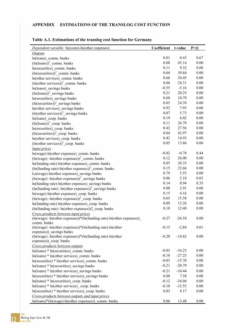
APPENDIX ESTIMATIONS OF THE TRANSLOG COST FUNCTION

Table A.1. Estimations of the translog cost function for Germany

Dependent variable: ln(costs)-ln(other expenses) Coefficient t-value P>|t| Outputs ln(loans)_comm. banks 0.01 0.43 0.67 (ln(loans))2_comm. banks 0.08 45.14 0.00 ln(securities)_comm. banks 0.11 9.32 0.00 (ln(securities))2_comm. banks 0.04 39.84 0.00 ln(other services)_comm. banks 0.66 34.45 0.00 (ln(other services))2_comm. banks 0.06 24.31 0.00 ln(loans)_savings banks -0.55 -5.16 0.00 (ln(loans))2_savings banks 0.21 20.25 0.00 ln(securities)_savings banks 0.60 10.79 0.00 (ln(securities))2_savings banks 0.05 24.39 0.00 ln(other services)_savings banks 0.92 7.93 0.00 (ln(other services))2_savings banks 0.07 5.73 0.00 ln(loans)_coop. banks 0.19 6.02 0.00 (ln(loans))2_coop. banks 0.11 26.79 0.00 ln(securities)_coop. banks 0.42 27.56 0.00 (ln(securities))2_coop. banks 0.04 42.97 0.00 ln(other services)_coop. banks 0.42 14.93 0.00 (ln(other services))2_coop. banks 0.05 13.86 0.00 Input prices ln(wage)-ln(other expenses)_comm. banks -0.02 -0.78 0.44 (ln(wage) -ln(other expenses))2_comm. banks 0.12 26.00 0.00 ln(funding rate)-ln(other expenses)_comm. banks 0.85 28.35 0.00 (ln(funding rate)-ln(other expenses))2_comm. banks 0.15 22.66 0.00 Ln(wage)-ln(other expenses)_savings banks 0.79 5.55 0.00 (ln(wage) -ln(other expenses))2_savings banks 0.06 2.18 0.03 ln(funding rate)-ln(other expenses)_savings banks 0.14 0.94 0.35 (ln(funding rate) -ln(other expenses))2_savings banks 0.08 2.91 0.00 ln(wage)-ln(other expenses)_coop. banks 0.15 4.16 0.00 (ln(wage) -ln(other expenses))2_coop. banks 0.65 15.58 0.00 ln(funding rate)-ln(other expenses)_coop. banks 0.09 15.26 0.00 (ln(funding rate) -ln(other expenses))2_coop. banks 0.10 12.40 0.00 Cross-products between input prices (ln(wage) -ln(other expenses))*(ln(funding rate)-ln(other expenses))_ comm. banks

-0.27 -26.54 0.00

(ln(wage) -ln(other expenses))*(ln(funding rate)-ln(other expenses))_savings banks

-0.15 -2.84 0.01

(ln(wage) -ln(other expenses))*(ln(funding rate)-ln(other expenses))_coop. banks

-0.20 -14.82 0.00

Cross-products between outputs ln(loans) * ln(securities)_comm. banks -0.03 -16.25 0.00 ln(loans) * ln(other services)_comm. banks -0.10 -27.25 0.00 ln(securities) * ln(other services)_comm. banks -0.03 -15.70 0.00 ln(loans) * ln(securities)_savings banks -0.21 -20.79 0.00 ln(loans) * ln(other services)_savings banks -0.21 -10.44 0.00 ln(securities) * ln(other services)_savings banks 0.08 7.58 0.00 ln(loans) * ln(securities)_coop. banks -0.12 -34.04 0.00 ln(loans) * ln(other services)_ coop. banks -0.10 -15.55 0.00 ln(securities) * ln(other services)_coop. banks 0.03 9.17 0.00 Cross-products between outputs and input prices ln(loans)*(ln(wage)-ln(other expenses))_comm. banks 0.06 13.48 0.00


ln(loans)*(ln(funding rate)-ln(other expenses))_comm. banks -0.04 -8.27 0.00 ln(loans)*(ln(wage)-ln(other expenses))_savings banks 0.00 -0.11 0.91 ln(loans)*(ln(funding rate)-ln(other expenses))_savings banks 0.02 0.78 0.44 ln(loans)*(ln(wage)-ln(other expenses))_coop. banks 0.10 11.44 0.00 ln(loans)*(ln(funding rate)-ln(other expenses))_coop. banks -0.08 -8.09 0.00 ln(securities)*(ln(wage)-ln(other expenses))_comm. banks 0.03 11.11 0.00 ln(securities)*(ln(funding rate)-ln(other expenses))_comm. banks -0.04 -10.00 0.00 ln(securities)*(ln(wage)-ln(other expenses))_savings banks -0.10 -6.34 0.00 ln(securities)*(ln(funding rate)-ln(other expenses))_savings banks 0.06 3.88 0.00 ln(securities)*(ln(wage)-ln(other expenses))_coop. banks -0.06 -14.28 0.00 ln(securities)*(ln(funding rate)-ln(other expenses))_coop. banks 0.05 10.49 0.00 ln(other services)*(ln(wage)-ln(other expenses))_comm. banks -0.05 -9.36 0.00 ln(other services)*(ln(funding rate)-ln(other expenses))_comm. banks 0.04 6.74 0.00 ln(other services) *(ln(wage)-ln(other expenses))_savings banks 0.07 2.22 0.03 ln(other services)*(ln(funding rate)-ln(other expenses))_savings banks -0.06 -1.89 0.06 ln(other services)*(ln(wage)-ln(other expenses))_coop. banks -0.04 -4.48 0.00 ln(other services)*(ln(funding rate)-ln(other expenses))_coop. banks 0.03 2.79 0.01 Control variables ln(equity/assets)_comm. banks -0.15 -4.26 0.00 ln(equity/assets)2_comm. banks 0.01 1.96 0.05 ln(equity/assets)_savings banks 1.11 6.80 0.00 ln(equity/assets)2_savings banks 0.21 7.86 0.00 ln(equity/assets)_coop. banks 0.51 10.03 0.00 ln(equity/assets)2_coop. banks 0.10 11.86 0.00 dummy savings banks 2.63 6.12 0.00 dummy coop. banks -0.15 -13.49 0.00 Intercept 3.07 48.08 0.00 Number of observations 19,551 F(80, 19,470) 25,462.91 Adjusted R-square 0.99 Explanation: Coefficients of time dummies have not been shown.

33ECB



European Central Bank Working Paper Series

For a complete list of Working Papers published by the ECB, please visit the ECB’s website(http://www.ecb.int)

737 “Structural balances and revenue windfalls: the role of asset prices revisited” by R. Morris and L. Schuknecht, March 2007.

738 “Commodity prices, money and inflation” by F. Browne and D. Cronin, March 2007.

739 “Exchange rate pass-through in emerging markets” by M. Ca’ Zorzi, E. Hahn and M. Sánchez, March 2007.

740 “Transition economy convergence in a two-country model: implications for monetary integration” by J. Brůha and J. Podpiera, March 2007.

741 “Sectoral money demand models for the euro area based on a common set of determinants” by J. von Landesberger, March 2007.

742 “The Eurosystem, the US Federal Reserve and the Bank of Japan: similarities and differences” by D. Gerdesmeier, F. P. Mongelli and B. Roffia, March 2007.

743 “Credit market and macroeconomic volatility” by C. Mendicino, March 2007.

744 “International financial linkages of Latin American banks: the effects of political risk and deposit dollarisation” by F. Ramon-Ballester and T. Wezel, March 2007.

745 “Market discipline, financial integration and fiscal rules: what drives spreads in the euro area government bond market?” by S. Manganelli and G. Wolswijk, April 2007.

746 “U.S. evolving macroeconomic dynamics: a structural investigation” by L. Benati and H. Mumtaz, April 2007.

747 “Tax reform and labour-market performance in the euro area: a simulation-based analysis using the New Area-Wide Model” by G. Coenen, P. McAdam and R. Straub, April 2007.

748 “Financial dollarization: the role of banks and interest rates” by H. S. Basso, O. Calvo-Gonzalez and M. Jurgilas, May 2007.

749 “Excess money growth and inflation dynamics” by B. Roffia and A. Zaghini, May 2007.

750 “Long run macroeconomic relations in the global economy” by S. Dees, S. Holly, M. H. Pesaran and L. V. Smith, May 2007.

751 “A look into the factor model black box: publication lags and the role of hard and soft data in forecasting GDP” by M. Bańbura and G. Rünstler, May 2007.

752 “Econometric analyses with backdated data: unified Germany and the euro area” by E. Angelini and M. Marcellino, May 2007.

753 “Trade credit defaults and liquidity provision by firms” by F. Boissay and R. Gropp, May 2007.

754 “Euro area inflation persistence in an estimated nonlinear DSGE model” by G. Amisano and O. Tristani, May 2007.

755 “Durable goods and their effect on household saving ratios in the euro area” by J. Jalava and I. K. Kavonius, May 2007.

35ECB


756 “Maintaining low inflation: money, interest rates, and policy stance” by S. Reynard, May 2007.

757 “The cyclicality of consumption, wages and employment of the public sector in the euro area” by A. Lamo, J. J. Pérez and L. Schuknecht, May 2007.

758 “Red tape and delayed entry” by A. Ciccone and E. Papaioannou, June 2007.

759 “Linear-quadratic approximation, external habit and targeting rules” by P. Levine, J. Pearlman and R. Pierse, June 2007.

760 “Modelling intra- and extra-area trade substitution and exchange rate pass-through in the euro area” by A. Dieppe and T. Warmedinger, June 2007.

761 “External imbalances and the US current account: how supply-side changes affect an exchange rate adjustment” by P. Engler, M. Fidora and C. Thimann, June 2007.

762 “Patterns of current account adjustment: insights from past experience” by B. Algieri and T. Bracke, June 2007.

763 “Short- and long-run tax elasticities: the case of the Netherlands” by G. Wolswijk, June 2007.

764 “Robust monetary policy with imperfect knowledge” by A. Orphanides and J. C. Williams, June 2007.

765 “Sequential optimization, front-loaded information, and U.S. consumption” by A. Willman, June 2007.

766 “How and when do markets tip? Lessons from the Battle of the Bund” by E. Cantillon and P.-L. Yin, June 2007.

767 “Explaining monetary policy in press conferences” by M. Ehrmann and M. Fratzscher, June 2007.

768 “A new approach to measuring competition in the loan markets of the euro area” by M. van Leuvensteijn, J. A. Bikker, A. van Rixtel and C. Kok Sørensen, June 2007.

ISSN 1561081-0

9 7 7 1 5 6 1 0 8 1 0 0 5

Documents

A new approach to measuring competition in the loan markets of the