Turk J Elec Eng & Comp Sci

(2017) 25: 3827 – 3838

c⃝ TUBITAK

doi:10.3906/elk-1606-415

Turkish Journal of Electrical Engineering & Computer Sciences

http :// journa l s . tub i tak .gov . t r/e lektr ik/

Research Article

A new approach to pulse deinterleaving based on adaptive thresholding

Mostafa BAGHERI, Mohammad Hossein SEDAAGHI∗

Department of Electrical Engineering, Sahand University of Technology, Tabriz, Iran

Received: 25.06.2016 • Accepted/Published Online: 20.06.2017 • Final Version: 05.10.2017

Abstract: Since histogram-based methods are formed by some simple differences, they are very desirable for deinterleav-

ing. However, their main imperfection concerns recognizing complex pulse repetition interval (PRI) patterns like jittered

and staggered ones. In this paper, we present new thresholds to detect jittered and staggered PRI from histogram-based

methods even in complex circumstances such as noisy time of arrival (TOA), complex PRI patterns, and large missing

pulses. Simulation results demonstrate that our method can detect and extract constant, jittered, and staggered PRI

correctly. Moreover, the method is proved to be considerably robust and reliable at a missing pulses rate up to 30%.

Key words: Radar, electronic support, pulse repetition interval, deinterleaving, adaptive thresholding

1. Introduction

Radars are considered the enemy’s eyes and have an important role in gathering information. In order to

increase their performance to detect moving targets or to be invisible for electronic warfare (EW) systems,

radars change pulse width (PW), radio frequency (RF), and pulse repetition interval (PRI) even from pulse to

pulse. Therefore, detection of such radars in a dense environment with complex signals is very complicated.

EW is a military action that employs electromagnetic energy radiated by radars for surveillance, and

electronic attack in some cases.

EW has classically been divided into three major classes: electronic support (ES, also called ESM),

electronic attack (EA, or alternatively named electronic counter measures (ECMs)) and electronic protect (EP,

as well as being entitled as electronic counter countermeasures (ECCM)). The main function of ES systems is

to receive, measure, and deinterleave pulses, and then identify alternative threat emitters. EA systems are used

to interfere with the operation of radars and EP systems are employed to protect one’s own systems against an

enemy’s electronic attacks [1].

Unlike the radar receivers having complete knowledge about what they should receive, an EW receiver is

not aware of the enemy’s radar signals. Therefore, it has a passive antenna with a wideband receiver to ensure

that all targets are covered. When each pulse is received, five parameters are usually measured and saved as

pulse description/descriptor word (PDW): PW, RF, pulse amplitude (PA), angle of arrival (AOA), and TOA

[2]. They are sent to the main processor to be classified and deinterleaved. This step should be performed with

high accuracy and speed to obviate EW requirements for fast decisions and actions. Moreover, a large number

of missing pulses are encountered due to the presence of low probability of intercept (LPI) radars [2,3], the

existence of obstacles to receive signals, and overlapping pulses. Thus, the algorithms for deinterleaving should

not fail in the presence of a high rate of missing pulses.

∗Correspondence: sedaaghi@sut.ac.ir

3827

BAGHERI and SEDAAGHI/Turk J Elec Eng & Comp Sci

Deinterleaving algorithms are divided into two categories: single parametric [4–18] and multiple para-

metric [19–23]. In multiple-parameter algorithms, two or more parameters are used for deinterleaving, while

in single-parameter ones, only one parameter is utilized. Among all pulse parameters mentioned above, TOA

is of considerable interest since it leads to a key derived parameter called PRI, which represents the difference

of sequential TOAs of the received pulses [19]. Thus, methods that use TOA for deinterleaving have been the

focus of many studies. In the work by Mardia et al. [6], a histogram-based method was proposed based on

accumulation called cumulative differentials (CDIF). This method is a discrete method and uses differences to

form differential histograms. Milojevic et al. [7] tried to decrease the computational cost of the CDIF algorithm

by extracting PRIs in each difference level. Thus, the modified version was proposed as the sequential differen-

tials (SDIF). In the research by Orsi et al. [8], an FFT-based method was proposed to extract pulse repetition

frequency (PRF = 1/PRI). Rather than trying to deinterleave a received interleaved pulse train directly, this

method focuses solely on determining the number of pulse trains present and the frequency of each pulse train.

In the work by Perkins and Coat [9], the nonlinear problem of pulse train deinterleaving is mapped into that of

line detection in a plane. The image processing technique known as Hough transform is then applied. Yujun et

al. [10] proposed straightforward SDIF-based PRI estimation. The approach uses only simple operations like

addition and comparison to calculate the SDIF and peak-value-detection to obtain possible PRIs. Nishiguchi

et al. [18] proposed a method called modified PRI transform that is a nonlinear integral transform. It retains

the peaks corresponding to PRIs and completely suppresses the peaks of the subharmonics.

Among all techniques that use TOA for deinterleaving, histogram-based methods are very common

because they are reliable and since they are formed by some simple differences they are easy to implement.

However, their main drawback is that the traditional thresholds cannot detect complex PRI patterns [24].

In this paper, we introduce new thresholds to extract complex PRI patterns like jittered and staggered

PRIs from histogram-based methods. Simulation results prove that the proposed method outperforms the

existing algorithms even in complex and dense environments with high rates of noise and missing pulses.

The organization of the paper is as follows. In Section 2 are shown the main PRI patterns. Section 3

introduces the proposed method. The analysis and results of the simulations are discussed in Section 4. Finally,

Section 5 concludes the paper.

2. PRI patterns

There are three basic PRIs: constant, stagger, and jitter. Constant PRI means the peak variations in PRI

values are less than about 1% of the mean PRI [19]. The times of arrival in this sequence are

tj = (j − 1) τs + tφ; j = 1, . . . , N, (1)

where τs is PRI and tφ is the reference time or phase.

Jittered PRI has large intentional PRI variations up to about 30% of the mean PRI with uniform

distribution:

tj = (j − 1) τc ± ατc + tφ; j = 1, . . . , N, (2)

where tj and τc denote TOA and the mean PRI, respectively. α is the deviation factor.

Staggered PRI uses two or more PRIs selected in a fixed sequence [19]. The sequence has M pulse gaps,

T1, . . . , TM repeated in M-count cycle: T j+M = Tj . The times of arrival are

3828

BAGHERI and SEDAAGHI/Turk J Elec Eng & Comp Sci

t1 = tφ

tj = tj−1 + Tj ; j = 2, . . . , N (3)

3. Proposed method

In order to extract PRIs from histograms, we propose two thresholds that are utilized simultaneously. The first

threshold is adaptive and extracts constant and staggered PRIs and the second one is applied to reveal the

jittered PRIs.

The proposed method is completed through four steps that will subsequently be discussed in detail.

3.1. Differential histogram forming

Let N interleaved pulses be recorded as [10]

ti ≡ {t1, t2, . . . , tN} (4)

where ti denotes TOA of the ith pulse and tj > ti > 0 ∀ j > i > 0.

All TOA differences from ti up to c adjacent pulses are computed:

∆t = tc+i − ti; i = 1, . . . , N − c (5)

where c increments by one until

tc+i − ti > PRImax (6)

Later, theith pulse is ignored and the process continues with other TOAs.

The time vector in a histogram is divided into K sections (also called bins):

τ i=τ1, . . . ,τK (7)

Bin’s width is computed by

b =PRImax−PRImin

K, (8)

where PRImaxPRImax and PRIminPRImaxdenote maximum and minimum values of acceptable PRI, respec-

tively. K is a constant indicating the number of bins.

PRImin, PRImax, and K are predefined values. Finally, each ∆t is placed into an appropriate bin

(τ1, . . . , τK).

3.2. Adaptive thresholding

In order to extract PRIs in a histogram of differences, a threshold is required. If the level of the threshold is

high, it will reduce the probability of correct detection. In contrast, a low level will lead to a higher false alarm

rate.

The main idea in the proposed method for thresholding is to control the required level adaptively. In order

to prevent the receiver from saturation by a large number of false alarms, some search radars employ constant

false alarm rate (CFAR). A histogram of differences can be modelled as received signal and noise in CFAR

3829

BAGHERI and SEDAAGHI/Turk J Elec Eng & Comp Sci

radars. In this histogram, each bin containing true PRIs is considered a true signal and the rest of the bins (not

carrying any PRI) are taken as noise. The assumption of uniform distribution gives good approximation for the

evaluation of the noise component [18]. Among all CFAR techniques, e.g., cell-averaging CFAR (CA-CFAR),

greatest of CFAR (GO-CFAR), and smallest of CFAR (SO-CFAR), CA-CFAR reveals the best performance in

homogeneous environments, specifically when considering noise (with uniform distribution) in the histogram

[25]. In CA-CFAR, an adaptive threshold for each bin (cell under test (CUT)) is derived by calculating the

mean value of the adjacent cells (reference cells) and multiplying it by a constant. Note that cells immediately

adjacent to the CUT, called guard cells, are excluded from the average [25]. Guard cells are used for separating

the CUT from the reference area in order to prevent true PRI from falsifying false adjacent bins made by noisy

TOA.

Therefore, the idea of adaptive threshold is driven using the following two steps:

1. calculate the mean value of each bin (averaging process):

M (i) =

i−G2∑

j=i−m2

R (j) +i+m

2∑j=i+G

2

R(j)

2(m−G); i = 1, . . . , k − x, (9)

where Rand m denote the bin’s value and number of reference cells, respectively, and G is the number

of guard cells. If x contains both guard and reference cells (x = m + G), to extract all stagger levels

correctly, x is derived by

(i+x

2)− (i− x

2) = x = 2f/b (10)

f is minimum PRI that is accepted for staggered radar and b is the bin’s width.

Thus, M is the mean value of xbins around the ith bin (CUT).

2. Compute the adaptive threshold as follows [25]:

T (i) = hM(i) (11)

T denotes the adaptive threshold and h is the threshold multiplier, obtained by

h = m(p

−1m

fa − 1)

(12)

where m is the number of reference cells and pfa is the probability of a false alarm.

3.3. Constant and staggered PRIs extraction

After applying the threshold, the bins exceeding the threshold are considered valid PRIs. To specify whether

they are constant or staggered, the following scale is used:

Si =Tw

( τib )=

bTw

τi; i = 1, . . . ,K, (13)

3830

BAGHERI and SEDAAGHI/Turk J Elec Eng & Comp Sci

where Tw and τi denote the last TOA and candidate PRI, respectively. By this scale, we can distinguish

constant PRIs from staggered ones. For example, if there exists staggered radar with M levels, the bins

indicating these levels will have magnitude equal(Tw/Ts)

M , where Ts = T1 + . . .+ TM . Therefore,

{τi = constant PRI |R (i) > (1/2)Si

τ i = staggered PRI |R (i) < (1/2)Si

(14)

where R(i) is the magnitude of the ith bin.

Since jittered PRI and histogram noise have the same distribution (uniform), jittered PRI behaves like

noise and the adaptive threshold cannot detect it. Thus, another threshold needs to be used to detect the PRI

of jittered radars.

3.4. Second threshold

After detecting/extracting constant and staggered PRIs, their corresponding bins are removed. Accordingly,

only jittered radars will reside in the histogram. Another threshold is then needed to detect jittered PRIs. Bin

magnitude related to jittered PRI is

Aτ =Ac

w; −ατc < τ < +ατc (15)

where Ac =Tw

τcand w = 2ατc

b ; thus,

Aτ =Twb

2ατ2c; −ατc < τ < +ατc (16)

Since the adaptive threshold has more flatness compared to bin magnitude (because of cell averaging) and

decreases the rate of false alarms, the second threshold is applied on the adaptive one. Therefore, the second

threshold should have the same offset:

γ (i) = h

(Twb

2ατ2i

); i = 1, . . . ,K (17)

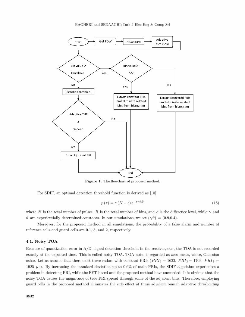
h is threshold multiplier used in the adaptive threshold. The flowchart of the proposed method is depicted in

Figure 1.

4. Simulation and analysis

There are many algorithms to deinterleave repetitive pulse trains. Nevertheless, the SDIF algorithm [7] and

FFT-based method [8] are very common. Other methods have some disadvantages such as being time consuming

[12], unreliable in the presence of noise [14], and not suitable for today’s harsh circumstances.

In order to compare the performance of the proposed method against these algorithms, the results of the

simulation experiments are presented. Note that the FFT-based method detects the PRF of each pulse train.

Simulation results of this method are presented in the frequency domain.

In this section, we will investigate complicated scenarios such as existing noisy TOAs, staggered and

jittered PRI, missing pulses, and mixed signals.

3831

BAGHERI and SEDAAGHI/Turk J Elec Eng & Comp Sci

Figure 1. The flowchart of proposed method.

For SDIF, an optimal detection threshold function is derived as [10]

p (τ) = γ (N − c) e−τ/ϑB (18)

where N is the total number of pulses, B is the total number of bins, and c is the difference level, while γ and

ϑ are experientially determined constants. In our simulations, we set (γϑ) = (0.9,0.4).

Moreover, for the proposed method in all simulations, the probability of a false alarm and number of

reference cells and guard cells are 0.1, 8, and 2, respectively.

4.1. Noisy TOA

Because of quantization error in A/D, signal detection threshold in the receiver, etc., the TOA is not recorded

exactly at the expected time. This is called noisy TOA. TOA noise is regarded as zero-mean, white, Gaussian

noise. Let us assume that there exist three radars with constant PRIs (PRI1 = 1633, PRI2 = 1703, PRI3 =

1925 µs). By increasing the standard deviation up to 0.6% of main PRIs, the SDIF algorithm experiences a

problem in detecting PRI, while the FFT-based and the proposed method have succeeded. It is obvious that the

noisy TOA causes the magnitude of true PRI spread through some of the adjacent bins. Therefore, employing

guard cells in the proposed method eliminates the side effect of these adjacent bins in adaptive thresholding

3832

BAGHERI and SEDAAGHI/Turk J Elec Eng & Comp Sci

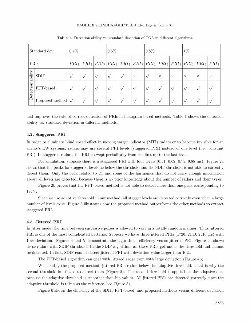
Table 1. Detection ability vs. standard deviation of TOA in different algorithms.

Standard dev. 0.4% 0.6% 0.8% 1%

PRIs PRI1 PRI2 PRI3 PRI1 PRI2 PRI3 PRI1 PRI2 PRI3 PRI1 PRI2 PRI3

Detection

ability

SDIF√ √ √ √ √

×√

× × × × ×

FFT-based√ √ √ √ √ √ √ √ √ √ √ √

Proposed method√ √ √ √ √ √ √ √ √ √ √ √

and improves the rate of correct detection of PRIs in histogram-based methods. Table 1 shows the detection

ability vs. standard deviation in different methods.

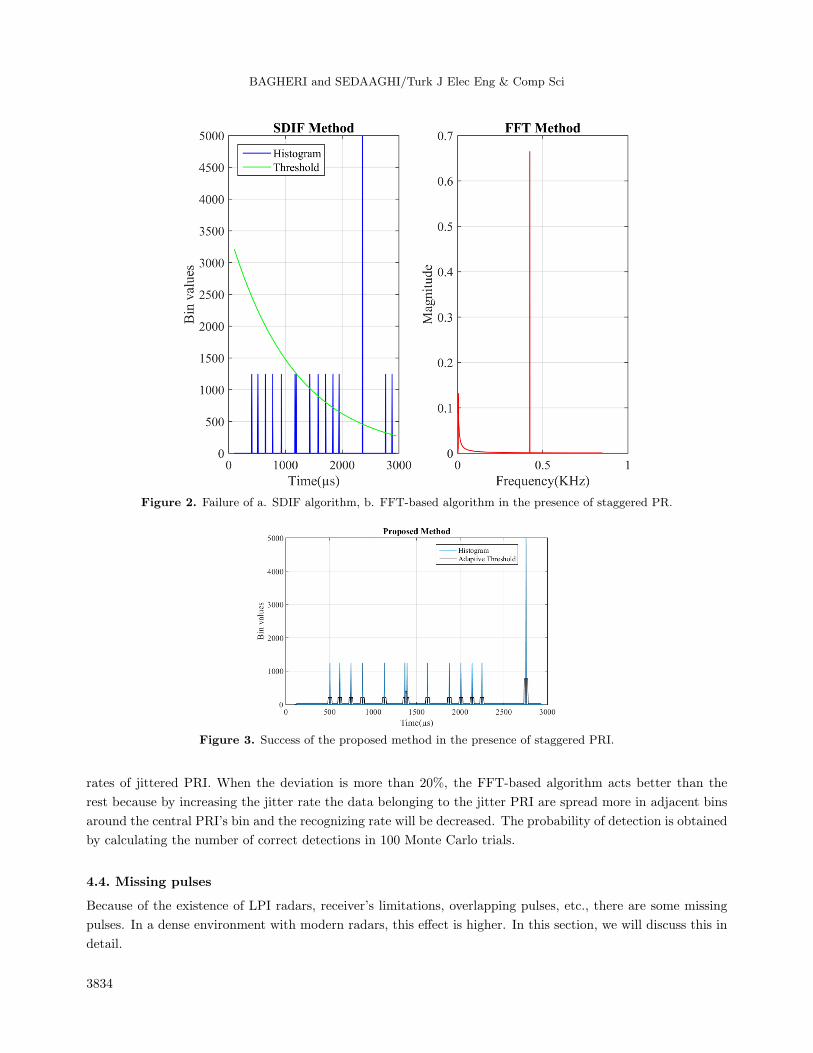
4.2. Staggered PRI

In order to eliminate blind speed effect in moving target indicator (MTI) radars or to become invisible for an

enemy’s EW systems, radars may use several PRI levels (staggered PRI) instead of one level (i.e. constant

PRI). In staggered radars, the PRI is swept periodically from the first up to the last level.

For simulation, suppose there is a staggered PRI with four levels (0.51, 0.62, 0.75, 0.88 ms). Figure 2a

shows that the peaks for staggered levels lie below the threshold and the SDIF threshold is not able to correctly

detect them. Only the peak related to Ts and some of the harmonics that do not carry enough information

about all levels are detected, because there is no prior knowledge about the number of radars and their types.

Figure 2b proves that the FFT-based method is not able to detect more than one peak corresponding to

1/Ts .

Since we use adaptive threshold in our method, all stagger levels are detected correctly even when a large

number of levels exist. Figure 3 illustrates how the proposed method outperforms the other methods to extract

staggered PRI.

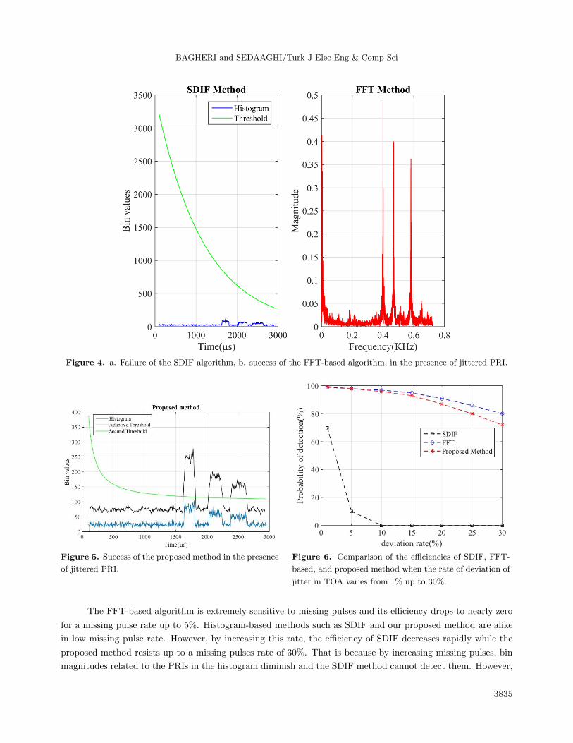
4.3. Jittered PRI

In jitter mode, the time between successive pulses is allowed to vary in a totally random manner. Thus, jittered

PRI is one of the most complicated patterns. Suppose we have three jittered PRIs (1720, 2140, 2510 µs) with

10% deviation. Figures 4 and 5 demonstrate the algorithms’ efficiency versus jittered PRI. Figure 4a shows

these radars with SDIF threshold. In the SDIF algorithm, all these PRIs get under the threshold and cannot

be detected. In fact, SDIF cannot detect jittered PRI with deviation value larger than 10%.

The FFT-based algorithm can deal with jittered radar even with large deviation (Figure 4b).

When using the proposed method, jittered PRIs reside below the adaptive threshold. That is why the

second threshold is utilized to detect them (Figure 5). The second threshold is applied on the adaptive one,

because the adaptive threshold is smoother than bin values. All jittered PRIs are detected correctly since the

adaptive threshold is taken as the reference (see Figure 5).

Figure 6 shows the efficiency of the SDIF, FFT-based, and proposed methods versus different deviation

3833

BAGHERI and SEDAAGHI/Turk J Elec Eng & Comp Sci

Figure 2. Failure of a. SDIF algorithm, b. FFT-based algorithm in the presence of staggered PR.

Figure 3. Success of the proposed method in the presence of staggered PRI.

rates of jittered PRI. When the deviation is more than 20%, the FFT-based algorithm acts better than the

rest because by increasing the jitter rate the data belonging to the jitter PRI are spread more in adjacent bins

around the central PRI’s bin and the recognizing rate will be decreased. The probability of detection is obtained

by calculating the number of correct detections in 100 Monte Carlo trials.

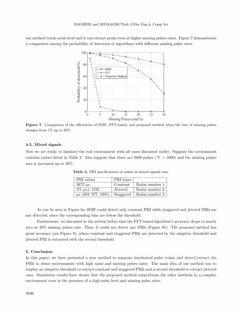
4.4. Missing pulses

Because of the existence of LPI radars, receiver’s limitations, overlapping pulses, etc., there are some missing

pulses. In a dense environment with modern radars, this effect is higher. In this section, we will discuss this in

detail.

3834

BAGHERI and SEDAAGHI/Turk J Elec Eng & Comp Sci

Figure 4. a. Failure of the SDIF algorithm, b. success of the FFT-based algorithm, in the presence of jittered PRI.

Figure 5. Success of the proposed method in the presence

of jittered PRI.

Figure 6. Comparison of the efficiencies of SDIF, FFT-

based, and proposed method when the rate of deviation of

jitter in TOA varies from 1% up to 30%.

The FFT-based algorithm is extremely sensitive to missing pulses and its efficiency drops to nearly zero

for a missing pulse rate up to 5%. Histogram-based methods such as SDIF and our proposed method are alike

in low missing pulse rate. However, by increasing this rate, the efficiency of SDIF decreases rapidly while the

proposed method resists up to a missing pulses rate of 30%. That is because by increasing missing pulses, bin

magnitudes related to the PRIs in the histogram diminish and the SDIF method cannot detect them. However,

3835

BAGHERI and SEDAAGHI/Turk J Elec Eng & Comp Sci

our method tracks noise level and it can extract peaks even at higher missing pulses rates. Figure 7 demonstrates

a comparison among the probability of detection of algorithms with different missing pulse rates.

Figure 7. Comparison of the efficiencies of SDIF, FFT-based, and proposed method when the rate of missing pulses

changes from 1% up to 30%.

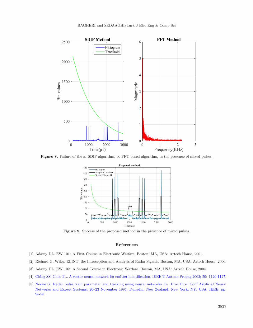
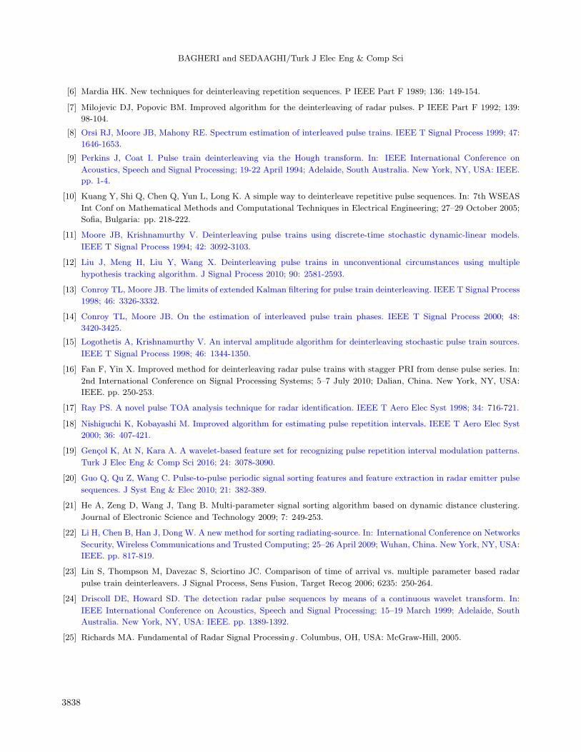
4.5. Mixed signals

Now we are ready to simulate the real environment with all cases discussed earlier. Suppose the environment

contains radars listed in Table 2. Also suppose that there are 5000 pulses (N = 5000) and the missing pulses

rate is increased up to 30%.

Table 2. PRI specifications of radars in mixed signals case.

PRI values PRI types2672 µs Constant Radar number 15% µs± 1533 Jittered Radar number 2µs (893, 977, 1085) Staggered Radar number 3

As can be seen in Figure 8a, SDIF could detect only constant PRI while staggered and jittered PRIs are

not detected, since the corresponding bins are below the threshold.

Furthermore, we discussed in the section before that the FFT-based algorithm’s accuracy drops to nearly

zero at 30% missing pulses rate. Thus, it could not detect any PRIs (Figure 8b). The proposed method has

great accuracy (see Figure 9), where constant and staggered PRIs are detected by the adaptive threshold and

jittered PRI is extracted with the second threshold.

5. Conclusion

In this paper, we have presented a new method to separate interleaved pulse trains and detect/extract the

PRIs in dense environments with high noise and missing pulses rates. The main idea of our method was to

employ an adaptive threshold to extract constant and staggered PRIs and a second threshold to extract jittered

ones. Simulation results have shown that the proposed method outperforms the other methods in a complex

environment even in the presence of a high noise level and missing pulse rates.

3836

BAGHERI and SEDAAGHI/Turk J Elec Eng & Comp Sci

Figure 8. Failure of the a. SDIF algorithm, b. FFT-based algorithm, in the presence of mixed pulses.

Figure 9. Success of the proposed method in the presence of mixed pulses.

References

[1] Adamy DL. EW 101: A First Course in Electronic Warfare. Boston, MA, USA: Artech House, 2001.

[2] Richard G. Wiley. ELINT, the Interception and Analysis of Radar Signals. Boston, MA, USA: Artech House, 2006.

[3] Adamy DL. EW 102: A Second Course in Electronic Warfare. Boston, MA, USA: Artech House, 2004.

[4] Ching SS, Chin TL. A vector neural network for emitter identification. IEEE T Antenn Propag 2002; 50: 1120-1127.

[5] Noone G. Radar pulse train parameter and tracking using neural networks. In: Proc Inter Conf Artificial Neural

Networks and Expert Systems; 20–23 November 1995; Dunedin, New Zealand. New York, NY, USA: IEEE. pp.

95-98.

3837

BAGHERI and SEDAAGHI/Turk J Elec Eng & Comp Sci

[6] Mardia HK. New techniques for deinterleaving repetition sequences. P IEEE Part F 1989; 136: 149-154.

[7] Milojevic DJ, Popovic BM. Improved algorithm for the deinterleaving of radar pulses. P IEEE Part F 1992; 139:

98-104.

[8] Orsi RJ, Moore JB, Mahony RE. Spectrum estimation of interleaved pulse trains. IEEE T Signal Process 1999; 47:

1646-1653.

[9] Perkins J, Coat I. Pulse train deinterleaving via the Hough transform. In: IEEE International Conference on

Acoustics, Speech and Signal Processing; 19-22 April 1994; Adelaide, South Australia. New York, NY, USA: IEEE.

pp. 1-4.

[10] Kuang Y, Shi Q, Chen Q, Yun L, Long K. A simple way to deinterleave repetitive pulse sequences. In: 7th WSEAS

Int Conf on Mathematical Methods and Computational Techniques in Electrical Engineering; 27–29 October 2005;

Sofia, Bulgaria: pp. 218-222.

[11] Moore JB, Krishnamurthy V. Deinterleaving pulse trains using discrete-time stochastic dynamic-linear models.

IEEE T Signal Process 1994; 42: 3092-3103.

[12] Liu J, Meng H, Liu Y, Wang X. Deinterleaving pulse trains in unconventional circumstances using multiple

hypothesis tracking algorithm. J Signal Process 2010; 90: 2581-2593.

[13] Conroy TL, Moore JB. The limits of extended Kalman filtering for pulse train deinterleaving. IEEE T Signal Process

1998; 46: 3326-3332.

[14] Conroy TL, Moore JB. On the estimation of interleaved pulse train phases. IEEE T Signal Process 2000; 48:

3420-3425.

[15] Logothetis A, Krishnamurthy V. An interval amplitude algorithm for deinterleaving stochastic pulse train sources.

IEEE T Signal Process 1998; 46: 1344-1350.

[16] Fan F, Yin X. Improved method for deinterleaving radar pulse trains with stagger PRI from dense pulse series. In:

2nd International Conference on Signal Processing Systems; 5–7 July 2010; Dalian, China. New York, NY, USA:

IEEE. pp. 250-253.

[17] Ray PS. A novel pulse TOA analysis technique for radar identification. IEEE T Aero Elec Syst 1998; 34: 716-721.

[18] Nishiguchi K, Kobayashi M. Improved algorithm for estimating pulse repetition intervals. IEEE T Aero Elec Syst

2000; 36: 407-421.

[19] Gencol K, At N, Kara A. A wavelet-based feature set for recognizing pulse repetition interval modulation patterns.

Turk J Elec Eng & Comp Sci 2016; 24: 3078-3090.

[20] Guo Q, Qu Z, Wang C. Pulse-to-pulse periodic signal sorting features and feature extraction in radar emitter pulse

sequences. J Syst Eng & Elec 2010; 21: 382-389.

[21] He A, Zeng D, Wang J, Tang B. Multi-parameter signal sorting algorithm based on dynamic distance clustering.

Journal of Electronic Science and Technology 2009; 7: 249-253.

[22] Li H, Chen B, Han J, Dong W. A new method for sorting radiating-source. In: International Conference on Networks

Security, Wireless Communications and Trusted Computing; 25–26 April 2009; Wuhan, China. New York, NY, USA:

IEEE. pp. 817-819.

[23] Lin S, Thompson M, Davezac S, Sciortino JC. Comparison of time of arrival vs. multiple parameter based radar

pulse train deinterleavers. J Signal Process, Sens Fusion, Target Recog 2006; 6235: 250-264.

[24] Driscoll DE, Howard SD. The detection radar pulse sequences by means of a continuous wavelet transform. In:

IEEE International Conference on Acoustics, Speech and Signal Processing; 15–19 March 1999; Adelaide, South

Australia. New York, NY, USA: IEEE. pp. 1389-1392.

[25] Richards MA. Fundamental of Radar Signal Processing . Columbus, OH, USA: McGraw-Hill, 2005.

3838