Embed Size (px)
Citation preview

Portland State University Portland State University
PDXScholar PDXScholar
Dissertations and Theses Dissertations and Theses
1989
A new approach to state minimization of finite state A new approach to state minimization of finite state
machines machines
William Yue Zhao Portland State University
Follow this and additional works at: https://pdxscholar.library.pdx.edu/open_access_etds
Part of the Electrical and Computer Engineering Commons
Let us know how access to this document benefits you.
Recommended Citation Recommended Citation Zhao, William Yue, "A new approach to state minimization of finite state machines" (1989). Dissertations and Theses. Paper 3951. https://doi.org/10.15760/etd.5835
This Thesis is brought to you for free and open access. It has been accepted for inclusion in Dissertations and Theses by an authorized administrator of PDXScholar. Please contact us if we can make this document more accessible: [email protected].

AN ABSTRACT OF TIIE TIIESIS OF William Yue Zhao for the
Master of Science in Electrical Engineering presented February 28, 1989.
Title: A New Approach to State Minimization of Finite State Machines.
APPROVED BY THE MEMBERS OF THE THESIS COMMITTEE:
Marek A. Pt owski
Robert L. Broussard
A complete program to ease the task of large scale Finite State Machine (FSM)
minimization presented in this thesis: TDFM (Two Dimensional FSM Minimizer), is a
part of the DIADES system. DIADES is an Automatic Design Synthesis System whose
development in the Department of Electrical Engineering at Portland State University is
supported in part by a research grant from SHARP Microelectronics Technology.
In compliance with the requirement of the DIADES system, the program TDFM
accepts two types of FSM formats of input data, .stab (state table) and .kiss (Keep the
Internal States Simple). TDFM's minimization procedures include the input based state
minimization (column minimization) and internal state based minimization (row minimi-

2
zation). As the major contribution of the program TDFM and this thesis, it has been pro
ven that this new type of minimization procedure, the column minimization, is possible
in the entire state minimization process and is as necessary as the traditional row minimi
zation. Furthermore, both of these two types of minimization can be done basically by
the same routines after some modification.
TDFM performs these two minimization processes in series, and iterates these
two procedures until there are no more compatible inputs or present states in the final
form of the machine. In other words, it generates an equivalent machine M*, which has
the minimal numbers of columns and rows. The optimal machine M* can also com
pletely replace the initial machine M 0 for the next design stages in the DIADES system.
It is the goal of the processes mentioned above to minimize the area of the VLSI circuit,
increase the speed, and improve the reliability.
These two minimization procedures basing on the state table are iterately per
formed through the following steps:
(1) find all of the compatible pairs of present states or inputs, by detecting
corresponding compatible conditions for each minimization process.
(2) generate all of the compatible groups (CG) for either the input columns
(CGI) or the present state rows (COP) and focus on those maximal compa
tible groups.
(3) create the closed and complete covering (CC) sets and then search out one
set of the minimal closed and complete covering (MCC) of either the
input columns (MCCI) or present state rows (MCCP) from those CGs
especially from those maximal CGs after each minimization process.
Finally, after the iteration of above minimization process steps, the last created
MCCI and MCCP forming from the most recently created state table are the optimal
minimal closed and complete coverings (OMCC) of input columns (OMCCI) and present

3
state rows (OMCCP).
For the purpose of searching for all the CGs in step 2, and for the MCCs (espe
cially for the OMCC) in step 3 during column minimization and row minimization as
well as in the additional procedure of column minimization (the input combinational
logic encoding), the program TDFM employs a universal Artificial Intelligence subrou
tine MULTCOM. This subroutine is used to list all of the CGs (first call for both column
and row minimizations described above) and later on to search out the MCCs (second
call) as well as to search for the MCC in the input encoding by using different specified
cost functions complemented by the respective quality functions and the selected search
ing strategies.
This thesis discusses the TDFM program in CHAPTER II and its main subroutine
MUL TCOM in CHAPTER IV in order to explain the entire minimization process.
During the development of the program TDFM, I obtained essential direction and
concern from my adviser Dr. Marek Perkowski and the help for understanding the rou
tine MUL TCOM from my colleague, Jiuling Liu. Here, I sincerely thank them for their
help. Without this help, the program TDFM may have been impossible.
Electrical Engineering Department
Portland State University
William Y. Zhao
A NEW APPROACH TO STATE MINIMIZATION OF
FINITE ST ATE MACHINES
by
WILLIAM YUE ZHAO
A thesis submitted in partial fulfillment of the the requirements for the degree of
MASTER OF SCIENCE in
ELECTRICAL ENGINEERING
Portland State University
1989

TO THE OFFICE OF GRADUATE STUDIES:
The members of the Committee approve the thesis of William Yue Zhao presented
February 28, 1989.
APPROVED:
Rolf Schaumann, Coordinator, Electrical Engineering
Bernard Ross, Vice Provost for Graduate Studies
TABLE OF CONTENTS
........................................................................................................................ PAGE
LIST OF TABLES ...................................................................................................... v
LIST OF FIGURES .................................................................................................... vu
MA TIIEMA TICAL SYMBOLS ................................................................................ ix
NOTICES.................................................................................................................... x
CHAP'I'ER ................................................................................................................. PAGE
I INTRODUCTION .......................................................................................... 1
II TIIE PROGRAM : TWO DIMENSIONAL FSM
MINIMIZER TDFM ....................................................................................... 9
2.1. Principle of State Table Minimization ................................. :............. 10
2.2. State Minimization Based On the Inputs
(Column minimization) ................................................................... 25
2.3. State Minimization Based On the Internal States
(Row Minimization) ....................................................................... 31
2.4. Input Signal Combinational Encoding ............................................... 36
III FORMATS OF FINITE ST A TE MACHINES .............................................. 44
3.1. Translation of Input Data Formats from .kiss to .stab ....................... 45
3.2. Translation of Input Data Formats from .liss to .stab ........................ 50
3.3. Specification of Input Files ........................................ ........................ 57
iv
CHAPTER PAGE
IV DESCRIPTION OF ROUTINE MULTCOM .............................................. 61
4.1. Selection of Strategies, Parameters and Size
Limitation of the Tree ..... ............ .. ...... .. .. .. ........ ...... ........ ...... ........ .. .. .. 61
4.2. Call to MUL TCOM for Finding All Compatible Groups ................. 66
4.3. Call to MUL TCOM for Creating MCCs .......................................... 70
4.4. Call to MUL TCOM for Input Combinational Covering .................. 82
V CONCLUSION ................................................................................ .............. 87
REFERENCES ........................................................................................................... 90
APPENDIX : USERS MANUAL .............................................................................. 92
LIST OF TABLES
TABLE PAGE
I An Initial State Table of Mealy Machine M 0 ............................................. 26
II Merger List ZGOD from State TABLE I for
Column Minimization .............................................................................. .. 28
ID List of Compatible Groups TAB IMP from State TABLE I ....................... 29
IV New State Table M 1 Created from TABLE I
after Column Minimization ....................................................................... 30
V Merger List ZGOD Created from TABLE IV
for Row Minimization ............................................................................... 33
VI List of Compatible Groups from State TABLE IV ................................... 34
VII New State Table M 2 Created from TABLE IV
after Row Minimization ............................................................................. 34
VIII Optimal State Table M* after Iteration of Minimizations .. .... .. .. .. .. .. .... .. .. 35
IX Process of Input Group Collection in List CGG ................................ ........ 37
X Code Table Created from Accumulation of
Input Compatible Groups ........................................................................... 38
XI Process of Tabulation for Encoding Output Function Fm ......................... 41
XII List of Compatible Groups from State Space in Figure 12(a) .................. 42
XIII Standard .kiss Formatted File ... ........ .. ........ .. .. .. ...... .... .. .. .... ...... ...... .. .. .. .. .. 46
XIV Modified .kiss Formatted Input File from TABLE XTII .......................... 49
vi
TABLE PAGE
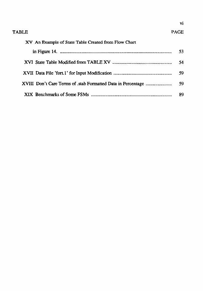
XV An Example of State Table Created from Flow Chart
in Figure 14. .............................................................................................. 53
XVI State Table Modified from TABLE XV .................................................. 54
XVII Data File 'fort. I' for Input Modification ................................................. 59
XVIII Don't Care Terms of .stab Formatted Data in Percentage ...................... 59
XIX Benchmarks of Some FSMs .................................................................... 89
LIST OF FIGURES
FIGURE PAGE
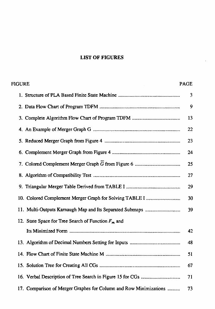
1. Structure of PLA Based Finite State Machine ....... .......................................... 3
2. Data Flow Chart of Program TDFM ................................................................ 9
3. Complete Algorithm Flow Chart of Program TDFM ...................................... 13
4. An Example of Merger Graph G ..................................................................... 22
5. Reduced Merger Graph from Figure 4 ............................................................ 23
6. Complement Merger Graph from Figure 4 ...................................................... 24
7. Colored Complement Merger Graph G from Figure 6 .................................... 25
8. Algorithm of Compatibility Test ..................................................................... 27
9. Triangular Merger Table Derived from TABLE I........................................... 29
10. Colored Complement Merger Graph for Solving TABLE I ..................... ...... 30
11. Multi-Outputs Karnaugh Map and Its Separated Submaps ............................ 39
12. State Space for Tree Search of Function Fm and
Its Minimized Form ................•....................................................................... 42
13. Algorithm of Decimal Numbers Setting for Inputs ........................................ 48
14. Flow Chart of Finite State Machine M ........................................................... 51
15. Solution Tree for Creating All CGs ................................................................ 67
16. Verbal Description of Tree Search in Figure 15 for CGs . .. ...... .... .. ...... .. .. .. .. .. 71
17. Comparison of Merger Graphes for Column and Row Minimizations .......... 73

Vlll
FIGURE PAGE
18. State Space for Tree Search of MCC .............................................................. 76
19. Solution Tree for Creating MCC .................................................................... 79
20. Verbal Description of Tree Search in Figure 19 for MCC ............................. 81
21. Solution Tree for Creating Covering of Function Fm ..................................... 85
22. Verbal Description of Tree Search in Figure 21 for MCC ............................. 86

MATHEMATICAL SYMBOLS
{a} : a group of single states.
{A} : a set of groups. Each group of this set can be represented by several states which belong to one group or be represented by the address of this group.
{A} = ~ : A is a empty set.
u: union.
n : intersection.
& : and, conjuncton.
v : or, disjunction.
EB : exclusive or.
a := b : a and b are compatible.
a = b: a and bare consistant.
A: the complement of A.
A ~B: A is included by B.
a e B : a is an element of B.
A I B: A conditioned on B.
a ~ b : b is implied by a.
CARD (A) : the number of elements in A.
l: (A) : the sum of the elements in A.
3 : there exists.
'if: for all.
m =fix (n) : m is the integer part of the real number n.
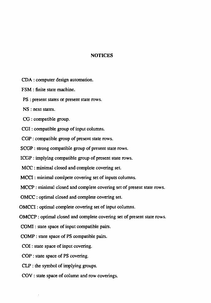
NOTICES
CDA : computer design automation.
FSM : finite state machine.
PS : present states or present state rows.
NS : next states.
CG : compatible group.
CGI : compatible group of input columns.
COP : compatible group of present state rows.
SCGP : strong compatible group of present state rows.
ICGP : implying compatible group of present state rows.
MCC : minimal closed and complete covering set.
MCCI : minimal comlpete covering set of inputs columns.
MCCP : minimal closed and complete covering set of present state rows.
OMCC: optimal closed and complete covering set.
OMCCI : optimal complete covering set of input columns.
OMCCP : optimal closed and complete covering set of present state rows.
COMI : state space of input compatible pairs.
COMP : state space of PS compatible pairs.
COi : state space of input covering.
COP : state space of PS covering.
CLP : the symbol of implying groups.
COV : state space of column and row coverings.

CHAPTER I
INTRODUCTION
The technology level used in circuit design rapidly progresses as the more sophis
ticated architectures used in VLSI (Very Large Scale Integration) computers and digital
circuit controllers are developed. This has especially been the case in the Eighties. One
component that plays a very important role in this respect (in the hardware design of
computers and other digital circuits) is the Finite State Machine (FSM). The state
minimization, state assignment, and Boolean minimization algorithm of FSM produce
much better results for the machine that have many don't care terms. Such machines can
be described in the initial specifications of control units (CU) in high-level synthesis sys
tems. This is, for instance, the case when the synthesis starts from the timing diagrams
(like for the control of the bus interface protocols), or when it uses constrained high-level
CU specifications.
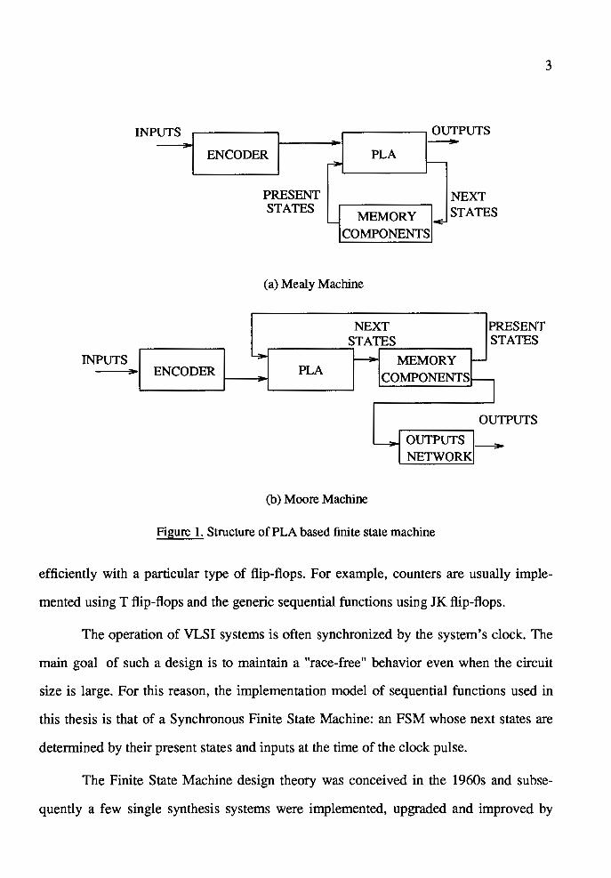
The hardware implementation of the FSM presented in this thesis consists of
three major components: input encoding circuit, combinational circuit as well as memory
components. These can be seen in the structures of the Mealy FSM model as shown in
Figure l(a) as well as in the Moore FSM model as shown in Figure l(b).
The difference between the Mealy and Moore machines is that the outputs of a
Mealy machine are dependent on both the present states and the inputs. This is accom
plished in the Mealy machine by using the present states given by the memory com
ponents as the functions of the machine states together with the primary inputs to make
up its primary outputs. On the other hand, the outputs of a Moore machine are deter
mined by the present states alone. The primary outputs of a Moore machine are created

2
from the memory components, via a separate output network. In both the Mealy and
Moore machines, the secondary states yielded by the combinational circuit form the next
states and become the input states to the memory components. The combinational circuit
and the memory components form a closed loop so that the internal states are changed in
the loop according to the transition functions. The memory components store the
representations of the states of the machine at any given time. The inputs to the memory
components are the next states and their outputs are the present states. The additional
input encoder is created to reduce the overall machine complexity. It is used to convert
those primary input signals into the secondary input signals according to the compatibil
ity of the primary input columns. The pertinent reduction procedure which is, of course,
not related to the memory components is introduced in § 2.4.
tives:
The VLSI implementation of a sequential circuit has to satisfy two major objec-
( 1) regular and structured design that can be supported by Computer Design
Automation (CDA) tools;
(2) size and performance optimization of the silicon implementation.
A PLA based or ROM based implementation of the FSM combinational circuit
and FSM based sequential circuit can be used to realize both of these goals. Since the
FSM memory components, as well as the PLAs, can be designed using regular structures,
the automation of FSM circuits design are allowable. Moreover, several techniques, such
as logic minimization and topological compaction, to design area-efficient PLAs have
been practical. Other realization of combinational functions, such as the standard cells,
Weinberger layouts, etc. are also applied on FSM design. A PLA-based FSM design can
then be optimized with respect to time-efficient performance.
The memory components of a FSM consist of a set of flip-flops. They can be of
several types, (Delay (D), Toggle (T), JK). Some functions can be implemented more
INP UTS
INPUTS I ENCODER I ~1 ,~UTS
JI ENCODER
PLA
PRESENT I STATES I MEMORY I
INEXT STATES
COMPONENTS
(a) Mealy Machine
NEXT STATES
~ ~ MEMORY -
PRESENT STATES
PLA COMPONENTS >--
UTPUTS
OUTPUTS ~
NETWORK
(b) Moore Machine
Figure 1. Structure of PLA based finite state machine
3
efficiently with a particular type of flip-flops. For example, counters are usually imple-
mented using T flip-flops and the generic sequential functions using JK flip-flops.
The operation of VLSI systems is often synchronized by the system's clock. The
main goal of such a design is to maintain a "race-free" behavior even when the circuit
size is large. For this reason, the implementation model of sequential functions used in
this thesis is that of a Synchronous Finite State Machine: an FSM whose next states are
determined by their present states and inputs at the time of the clock pulse.
The Finite State Machine design theory was conceived in the 1960s and subse
quently a few single synthesis systems were implemented, upgraded and improved by
4
several researchers. These research efforts had very little, if any, impact on the design
practice in the industrial environment during that period. The findings of these efforts
were not directly applicable to the computer realization. Another shortcoming of the
researches done during this period was that the implementation methodologies used in
their approaches did not take the exact optimization of designs into consideration.
Almost all research efforts in FSM state minimization begin with a state table
because it offers more clarity of the relationship of external and internal states, and so
far, the states can easily be translated from one table to the next. An example of such a
table is shown in TABLE I. The detailed description concerning state tables is given in §
2.2.
Paul and Unger [l] and Unger [2] have developed a general theory for the minim
ization of incomplete machines. Their method, however, for obtaining a minimal closed
covering involves a great deal of enumeration and inspection. Furthermore, their implica
tion graph only shows the implication between compatible pairs which obscures vital
information with respect to larger implied compatible present states containing more than
two states.
McCluskey [3], Pager [4], and Enrich [5] have developed ingenious methods for
minimizing a restricted class of incomplete FSM. Their techniques, however, are only
applicable to a very special class of machines.
Grasselli and Luccio [ 6] have presented an interesting approach by casting the
problem in the form of a linear integer program. Their minimization process which uses
the prime compatible present states and a closure covering table, however, is quite com
plex.
Luccio [7] improved the method from [ 6] by extending the definition of prime
compatible groups. His method, however, is quite lengthy and involves tedious pro
cedures.

5
As of the 1980s, most approaches to FSM design have began to concentrate on
circuit optimization and the computer design automation. Because of the progress that
has taken place in VLSI technology, research began to focus on FSM circuits having a
large number of states and inputs (for example, more than 50 present states and/or inputs)
as well as many don't care terms (over 50% of possible state transitions, and outputs).
A widely used program for the design of Finite State Machine is the PEG (PLA
Equation Generator), implemented by Gordon Hamachi, of UC Berkeley [8]. As an FSM
compiler, this program can translate the high level language description (the .peg format
input file specified by a flow chart) of a FSM into format .eqn by using the Moore
machine model. The FSM is represented by several logic equations in format .eqn.
Unfortunately, it deals with only the internal states minimization of the completely
specified machines. The result of this minimization, whatsoever, is not even minimal.
Moreover, it can be used for neither the state minimization of incompletely specified
machines nor for the design related optimization problem of these incompletely specified
machines.
In 1985, M. Perkowski and N. Nguyen [9] developed another FSM compiler,
SuperPEG: an even more powerful tool for state minimization. SuperPEG can accept
Moore and Mealy machine specifications and translate one form of representation into
the other. The outstanding contribution that SuperPEG made is that it is able to generate
all of the compatible groups of present state rows and select a minimal closed and com
plete covering for present state rows from the compatible internal state groups. It
employs a tree search approach with a cost function in order to cut off those tree
branches which are unable to lead to a minimal closed and complete covering of present
state rows. The routine MULTCOM, used in this compiler, is a problem-independent
Artificial Intelligence (Al) based tree-searching program. It can be personalized for vari
ous applications. During the state minimization, MUL TCOM has to be called twice. The

6
first calling to MULTCOM generates all compatible groups of present state rows. In the
second calling, a cost function is used to decide if the search on a certain branch of solu
tion tree should be retained or not. When a node is generated in the search process,
whose value of cost function exceeds (or equals) the cost of the tentative solution, then a
subtree starting from this node is cut-off and backtrack occurs. The other rules are based
on the properties of compatible (for instance the necessity to fulfill completeness condi
tion or closure condition for sets of compatible states and the general principles of cut-off
sets of nodes of the tree before their creation). The last property utilizes the concept of
operators. Application of an operator creates a new node of the tree. The operator antiCi
pates certain properties of descendant node before creating this node in the tree. The tree
size can be thus decreased by removing certain descendant nodes from the set of opera
tors to apply in the parent node, before actually opening it.
Considering the advantage of MULTCOM which yields the minimal solution out
of all solutions, especially when the state table involves a lot of don't care terms, the sub
routine MUL TCOM is also acceptable in the approach of this thesis. However, Super
PEG is not able to minimize the input columns of the state table; its solutions are actually
not optimal at this point.
In this thesis, the new ideas that the columns of the state table can also be minim
ized and the optimal solution is always carried out by the iteration of both column and
row minimization procedures are developed and presented. Usually, a number of
corresponding next states of some columns of the state table are combinable, when all of
these corresponding next states and outputs of these columns are consistent. This combi
nation occurs more frequently when there are many don't care terms in internal states and
outputs. As a result, the input column minimization should be considered in the entire
FSM minimization process. The possibilities of input column minimization should not
only be considered in the original state table, but also in the new state tables created by
7
each process of the present state minimizations mentioned above. This traditional present
state minimization is termed state row minimization in this thesis to distinguish it from
the input column minimization. After the result of column or row minimizations is
created, the program tests whether further minimization on another dimension (rows or
columns) is possible. If the answer is true, the result of this process becomes one minimal
complete covering for input columns or one minimal closed and complete covering for
present state rows, and so far, a new state table in which one dimension has been minim
ized is created and the next minimization process will be carried out in another dimen
sion. Otherwise, the last created results of column and row minimizations will become
the optimal solution. The optimal solution actually includes two parts: the optimal com
plete covering for input columns and the optimal closed and complete covering. Such an
optimal solution is, therefore, obtained only after the ultimately possible minimization
has been performed and the minimum state table has been created.
The detailed description of this new approach will be presented in CHAPTER II.
The new FSM minimization program TDFM has been implemented in support of the
approach presented in this thesis. The subroutine MUL TCOM is introduced in
CHAPTER IV. Even though there are other methods of performing the above minimiza
tions, such as using the graph coloring method [12] which minimizes only the input
columns, these methods discussed in the following chapters can not be applied for
minimization programming because of their shortcomings. To shorten the time perfor
mance of program TDFM, MUL TCOM has been adapted and used in this program for
present state row minimization, input column minimization and minimal covering for
binary input expressions encoding. The improvements done to the subroutine
MULTCOM to achieve these goals are also presented in CHAPTER II and CHAPTER
IV. In addition, several machines that have more complicated structures than the
machines presented in the previous approaches have been minimized: they have, for
example, more internal states, multi-bit inputs and outputs, and a higher percentage of

8
don't care terms. The specifications for these machines are presented in CHAPTER V.
CHAPTER II
THE PROGRAM : TWO DIMENSIONAL FSM MINIMIZER TDFM
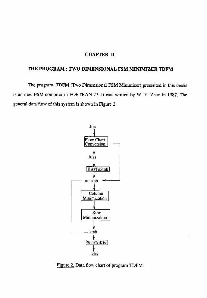
The program, TDFM (Two Dimensional FSM Minimizer) presented in this thesis
is an new FSM compiler in FORTRAN 77. It was written by W. Y. Zhao in 1987. The
general data flow of this system is shown in Figure 2 .
.liss
.------ .stab
Column Minimization
Row Minimization
~--.stab
StabToK.iss
.kiss
Figure 2. Data flow chart of program TDFM

10
The interconversion of the input data formats is presented in CHAPTER III. The
.kiss or .stab data file represents either a completely or an incompletely specified FSM.
The processes of both column and row minimizations are based only on the .stab format
ted Mealy state table.
Two types of minimizations, the column minimization and the row minimization,
are processed serially and iteratively until no more columns or rows can be minimized.
Similarly to SuperPEG, TDFM utilizes the procedure MULTCOM for tree search. The
difference is: MUL TCOM has been upgraded so that it will not only minimize the PS
rows but also minimize the input columns of the state tables and minimize the minimal
covering for the binary input encoding. Since these three tasks have different require
ments, TDFM can successfully deal with them respectively by using different strategies
and parameters. In the following sections, the improvements (such as suiting the input
data which have different styles, sizes, or formats, arranging the merger lists for the next
column or row minimization, collecting the input compatible groups for the binary input
expressions encoding, etc.), will be introduced. Some improvements in MULTCOM
(such as the application of particular prameters, the test of the closure condition for PS
row minimization, etc.), to match various tasks are also presented to explain the relation
ship between the main program TDFM and the subroutine MUL TCOM.
§ 2.1. PRINCIPLE OF ST ATE TABLE MINIMIZATIONS
After a .stab formatted input data table is presented, TDFM can start the minimi
zation procedures. As it has been mentioned, the most important improvement to TDFM
compared with those previous FSM minimizing methods is that TDFM can deal with two
types of the state minimization, the minimization based on the input columns and the
minimization based on the PS rows. Although both of them are intended to minimize the
structure of the state table, and the methodologies of these two kinds of minimization are

11
similar, or even the same in some points, they are quite different according to the princi
ple of minimization. The following definitions basing on Mealy state table are necessary
for the description of the appropriate problem formulation.
Definition (1 ):
A group of present states {si, ... ,sj} of machine M consists of a state compatible
~(COP), if and only if, under every input column Xr (1 ~ r ~ mx) the next states
{s'i,r. ... ,s'j,r} corresponding to all of the present state rows in the group {si, ... ,Sj} are
compatible (the corresponding next states belong to their parent present states) or are
consistent (the corresponding next states of the group either have the same value or are
don't-care terms) and the corresponding outputs {z'i,r•··.,z'j,r} are consistent bit by bit
(every corresponding bits of corresponding outputs either have the same value or are
don't-care terms).
Definition (2):
A group of input states {xi, .. .,Xj} of machine M consist of an input combinable
~ (CGn if and only if, under every present state rows Sr (1 ~ r ~ na) the next states
{s'r,i, .. .,s'r,j} corresponding to all of the input columns in this group {Xi,. . .,Xj} are con
sistent and the corresponding outputs {z'r,i, .. .,z'r,j} are also consistent bit by bit.
Property ( 1 ):
The combinational input state group is also called the input compatible group and
the addresses of the input states in this group are indicated by {ii,. .. ,ij} in this thesis.
Definition (3):
For a group of present states {Si, .. .,sj} if under a certain input column Xr the next
states s'i.r· .. .,s'j,r corresponding to all of the present state rows in the present state group
{si,. .. ,Sj} belong to another present states group {sp, .. .,sq}, and other next states
corresponding to the same present state rows satisfy the compatible condition according
to definition (1), then the group {si,. . .,sj} is considered to imply the group {s'i,r,. . .,s'j,r}.

If {sp, ... ,sq} is compatible, {si, ... ,sj} is called the implying compatible~ (ICGP).
Definition (4):
12
A set of compatible groups of machine M {Si, ... ,Sj} is overlap if the same ele
ments appear in different groups of this set.
Definition (5):
A set of compatible groups of present states (COP) of machine M satisfies the clo
sure condition, if each of its implied compatible groups (ICGP) is also included in a
group from this set as well.
Definition (6):
A set of compatible groups of machine M satisfies the completeness condition, if
each internal state or input state is contained in at least one group of this set.
Property (2):
A compatible group includes a certain number of elements. The quality of such a
CG is defined by Q, the number of its elements. A relatively maximal compatible group
has the highest Q value.
Definition (7):
A covering set which satisfies the conditions of both closure and completeness is
called a closed and complete covering set (CC) or a solution set.
Definition (8):
A solution set which satisfies the conditions of closure and completeness consists
of the minimum number of CGs with the relatively higher Q and less overlap is a
minimal solution set (MCC). Such a feasible solution set has the minimum cost value
(the number of CGs in this set) defined by CF.
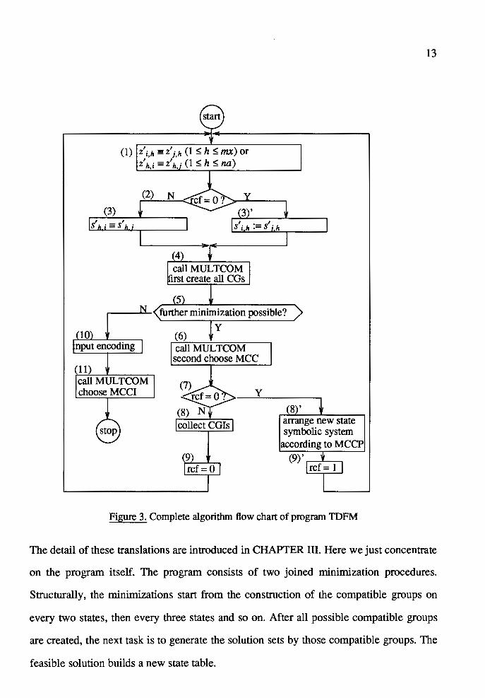
The complete algorithm for describing the behavior of the program TDFM is
presented in Figure 3. The procedures performed priorly and posteriorly to this program
are KissToStab and StabToKiss, if the input and required output files are .kiss formatted.
(1) lz'i,h = z'j,h (1 $; h $; mx) or z\i = z\; (1 $; h $; na)
N y
3)'
(4) call MULTCOM rst create all CGs
5 further minimization possible?
y 10
nput encoding
(11 call MULTCOM chooseMCCI
(6) call MULTCOM
second choose MCC
y
(8" arrange new state symbolic system
according to MCCP
(9)' i * i
ref= 1 --.-
Figure 3. Complete algorithm flow chart of program TDFM
13
The detail of these translations are introduced in CHAPTER III. Here we just concentrate
on the program itself. The program consists of two joined minimization procedures.
Structurally, the minimizations start from the construction of the compatible groups on
every two states, then every three states and so on. After all possible compatible groups
are created, the next task is to generate the solution sets by those compatible groups. The
feasible solution builds a new state table.
14
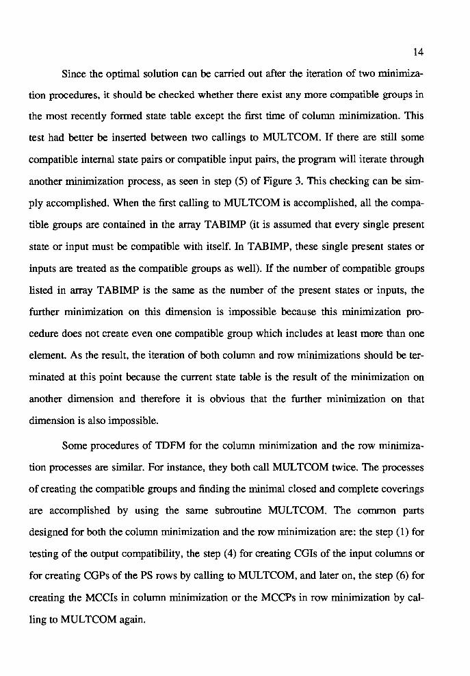
Since the optimal solution can be carried out after the iteration of two minimiza
tion procedures, it should be checked whether there exist any more compatible groups in
the most recently formed state table except the first time of column minimization. This
test had better be inserted between two callings to MUL TCOM. If there are still some
compatible internal state pairs or compatible input pairs, the program will iterate through
another minimization process, as seen in step (5) of Figure 3. This checking can be sim
ply accomplished. When the first calling to MUL TCOM is accomplished, all the compa
tible groups are contained in the array TAB IMP (it is assumed that every single present
state or input must be compatible with itself. In TAB IMP, these single present states or
inputs are treated as the compatible groups as well). If the number of compatible groups
listed in array TAB IMP is the same as the number of the present states or inputs, the
further minimization on this dimension is impossible because this minimization pro
cedure does not create even one compatible group which includes at least more than one
element. As the result, the iteration of both column and row minimizations should be ter
minated at this point because the current state table is the result of the minimization on
another dimension and therefore it is obvious that the further minimization on that
dimension is also impossible.
Some procedures of TDFM for the column minimization and the row minimiza
tion processes are similar. For instance, they both call MUL TCOM twice. The processes
of creating the compatible groups and finding the minimal closed and complete coverings
are accomplished by using the same subroutine MUL TCOM. The common parts
designed for both the column minimization and the row minimization are: the step (1) for
testing of the output compatibility, the step (4) for creating COis of the input columns or
for creating CGPs of the PS rows by calling to MULTCOM, and later on, the step (6) for
creating the MCCis in column minimization or the MCCPs in row minimization by cal
ling to MULTCOM again.

15
However, there exist also some differences between these two procedures. Partic
ularly, the step (3) for testing the compatibility of input state columns, the step (8) for
collecting the addresses of input CGis in the array COO, as well as the steps (10) and
(11) for input encoding are designed for column minimization alone. On the other hand,
the step (3)' for testing the PS compatibility, as well as the step (8)' for arranging the
new state symbolic system are designed for row minimization alone.
The compatibility conditions for NSs of these two procedures are entirely dif
ferent. This is because the nature of these two kinds of compatibilities are different. For
the row minimization, the compatibility of the internal state rows in the state table must
be tested as follows. For a compatible group of PS rows, every pair of the NSs and out
puts at the corresponding intersections of the selected rows and all columns must satisfy
the compatibility condition or they must satisfy the implied compatible condition. The
compatibility strictly follows the definition (1) for compatible groups (CGP) and also the
definition (3) for implied compatible groups (ICGP).
On the other hand, in the column minimization, for a group of input columns,
every corresponding NSs and outputs which can be arranged into a compatible group at
the intersections of the selected columns and all rows must have the same value or be
don't-care terms. The compatibility of input columns (CGI) are decided by definition
(2). The implied compatible groups do not exist in this procedure. Comparing the compa
tible conditions between column and row minimizations, the consistence conditions are
the same for the outputs, but the compatibility conditions are different on NSs. By chang
ing the compatible testing conditions, the same facilities, such as the merger list ZGOD
and the following of MULTCOM for creating the compatible groups, can be used for
both of these two minimizations for making the program shorter and more efficient. In
the column minimization, the reason that the term 'compatible' is borrowed from the
procedure of row minimization is that the merger list array ZGOD for creating the com-

16
patible pairs from the state table has been used in both row and column minimization
procedures (indicated by the step (1) and the step (3) or the step (3)' of Figure 3). The
detailed description of ZGOD and the different usages in these two procedures are intro
duced in § 2.2 and§ 2.3 respectively. This method has been proven very effective, easy
to be programmed and easy to be enhanced for dealing with relatively larger scale state
tables.
There is also some difference in the test of the closure and completeness condi
tions of the solution sets during the second MUL TCOM call. For instance, some implied
compatible groups (ICGP) might be chosen in the solution set in row minimization. The
test of closure and completeness must be carried out afterwards. In the second calling to
MULTCOM for the column minimization, the solution candidate test of CGis will not
include the closure condition, since all the CGis are naturally closed.
Even though the column and row minimization utilize the same subroutine
MULTCOM, there still exist some differences within the MUL TCOM. The analyses of
these problems can be found in CHAPTER IV.
Speaking of the nature of these differences, the state minimization based on
present state rows is a sequential logic reduction because the relationship of PSs and NSs
is actually the transition between the input and output of the sequential memory com
ponents. That is, when minimizing the number of PS rows, the NSs will be taken in con
sideration since they may relate to some other PSs and may affect the compatibility of
the PSs. Therefore, in the second calling to MUL TCOM, the test of the quality of the
internal state compatible groups (CGP) will include the closure, completeness and over
lapping of these CGPs with the other selected CGPs. However, in the column minimiza
tion, those NSs are not sequentially related to the input constraint conditions. The execu
tion of this minimization is absolutely a purely combinational logic reduction of the
corresponding NS/output units among those columns. Strictly speaking, this is not a com-

17
patibility problem but rather a simplification problem of combinational logic functions.
That is why, when the column minimization procedures are accomplished, an input
encoder must be inserted between the primary input states and the secondary input states
of the machine since the inputs are NOT reduced, but combined. An input encoding pro
cedure must be therefore used for this purpose in MUL TCOM correspondingly.
Consequently, the steps that carry out the column and row minimizations are as
follows.
( 1) Since these two minimization procedures use the same subroutine
MULTCOM, it is necessary to have a flag "ref' to distinguish the
processes of column and row minimizations. The routine will execute the
row minimization if this flag equals 'O'. Otherwise, it will execute the
column minimization if flag 'ref' equals '1 '. The column minimization
had better be performed first. The result of the column minimization (a
new state table) will become the input data file of the next step, the row
minimization. Then, after the row minimization process is executed, the
result of the row minimization (another new state table) is also used as the
input data file for the next column minimization. All of the state tables
created at each stage are stored as the records of the entire minimization
process.
(2) Search every corresponding NS/output units under every two rows or
every two columns in the state table to detect whether the two present
state rows or two input state columns are compatible according to
definitions (1) and (3) or definition (2). Definitions (4) and (5) correspond
only to the PS row minimization. The result of this step is to collect all the
compatible pairs.
(3) Generate all the compatible groups of PSs or inputs from all single states

18
and the compatible pairs created in the last step. Some of these CGs may
become the groups of the solution set. All the selected compatible groups
of inputs are represented by their addresses shown in the original state
table.
( 4) After the compatible groups have been created, check if further minimiza
tion is possible after each row or column minimization (notice that this
test is not necessary for the first time of row and column minimizations).
If true is returned, go to the step (6), and the next stage of iteration must
be taken. Otherwise, terminate the iteration. The last created MCCI and
MCCP sets are OMCCI and OMCCP (the optimal minimal complete cov
ering for input columns or the optimal minimal closed and complete cov
ering for PS rows).
(5) Execute the Input Encoding procedure. Call MUL TCOM to generate the
prime implicants indicated by the collection of CGI in step (3), and stop
the program.
(6) Search CCis or CCPs from CGis or CGPs, and subsequently, choose the
MCCI and the MCCP sets according to definition (8). The features of
MCCsetare:
(a) It must include the minimum number of groups in the solution set.
A non-minimum solution is never acceptable.
(b) Each selected address of CGI or CGP must be presented in a cer
tain group of the set (completeness). Closure and completeness are
the necessary conditions of a solution. Ideally, each input or PS
had better appear in only one group of the set. Such a solution set
is a so called non-overlapping solution according to definition (4).
For row minimization, this is usually not easy to achieve.

19
Build a new state table according to the MCCI or MCCP. Then, change
the value of the flag 'ref' and enter the next step of iteration of minimiza
tion i.e. go back to step ( 1 ).
In the previous approaches, a variety of methods for generating the CGs and,
therefore for finding the closed and complete coverings have been investigated aside
from using the subroutine MULTCOM. These approaches attempted to use different
methods to achieve this goal. A commonly acknowledged method is creating the merger
graph G derived from the triangular merger table.
Nripendra Biswas [10] in 1974 used this merger graph G solving the closed and
complete covering of PS row minimization. Then, Masotu Yamamoto [11] in 1980 used
both of the merger graph G and its complement graph G searching the MCCP in row
minimization. Later on, M. Perkowski and H. Uong [12] in 1987 introduced G searching
the MCCI for column minimization. Their method is to "color" the compatible input
columns in the same group according to their compatibility.
Essentially, these graph methods are used to create MCC by separating graph G
or its complement graph G into some constrained complete polygons for finding of the
compatible groups or incompatible groups. Such polygons are the so called Maximal
Cliques or Maximum Independent Sets of G or G, respectively.
For the column minimization, this method is very clear and it can easily illustrate
the nature of finding the complete coverings for input columns. Since every node in this
graph has a certain color, it will not appear in any other group if it has been assigned a
certain color. The groups finally make up the minimal complete coverings. Obviously,
this complete covering is never overlapped because each node can belong to only one
group. If the set has the smallest number of compatible groups and these compatible
groups do not overlap, this set is actually the minimal complete coverings in column
minimization process.

20
Basically, the graph method of finding the covering introduced in [12] is unable
to prove this covering's closure condition for implied compatible groups. Fortunately, in
column minimization, the 'implied' compatible group problem does not exist. According
to definition (2), the conditions of column compatibility point out that the NSs at the
corresponding intersections must have either the same value or at least one of them must
be a don't-care term. In other words, the NSs' compatibilities are not related to any other
PS groups not even to their own parent PS groups. Therefore the compatibility of input
columns in column minimization actually depends only on the relationship of the
corresponding NSs themselves.
Since the closure and completeness must be proven in any stage of row minimi
zation, this method is not able to complete the row minimization without further
modification. The modification for the merger graph is introduced in detail in CHAPTER
IV of this thesis and Figure 17 will illustrate an example of this.
The processes of the graph coloring and MUL TCOM are very different. After the
merger graph method creates those CGs it generates only one solution set at each time.
The CGs in the solution may not be the maximal. In other words, their quality Q (refer
ring to the Property (2) ) may be lower than some CGs which are not chosen to form this
solution. Therefore the cost of the solution (referring to the Property (3) ) may not be the
lowest. If someone wants to compare the costs of all solutions, the process of selecting
the solutions has to be applied many times until all of the solutions are created. As a con
trast, MUL TCOM creates all of the CGs also but then compares the numbers of elements
in every CGs (In column minimization, the number of don't-care terms in every binary
inputs are also be considered.) and gives the priority to the CGs which have higher Q
values in the solution set in the second calling to this subroutine. Therefore, such a solu
tion is minimal. The CGs which have lower Q values will not be used to create the solu
tions. In other words, these solutions are aborted before they are formed. Even though the

21
merger graph method can quickly create the solutions, in fact, calculating the qualities of
the existing CGs and the costs of the solutions will spend much longer time than creating
them. Consequently, the speed of MULTCOM is quite faster than the coloring graph
method for finding the MCCs when the size of the FSM is very large and the number of
solutions is increased sharply. Therefore, the subroutine MULTCOM has been applied
in the program TDFM considering the application of VLSI technology in FSM design.
Merger graph method, however, is still of benefit to clarify the compatibility of states or
inputs as well as the relationship of the completeness to those compatible groups of the
solution set. Therefore, this method is used to analyze the solution set of the machine
created by the program TDFM in this thesis.
The method of creating the merger graph is easy to learn. The graph G of the
column minimization has to be separated into some complete cliques to generate the
compatible groups (CGn. Figure 4 is a simple example of merger graph G. The steps to
draw a merger graph are:
(1) Put all of the input or PS decimal numbers in the nodes.
(2) Connect all of the compatible pairs of nodes.
(3) Decide the CGis in G, and formula (1):
(1)
is used. If a group of n nodes belong to a compatible group, the number of
the connections among these n nodes should be W. For instance, in Fig-
4(4-1) ure 4, a group {l,2,4,5) is a good one because n = 4 and W =
2 = 6.
The group {l,3,4) is not because n = 3 but there are only 2 connections.
It is clear that in graph G the nodes which are connected should belong to the
same group. This is shown in Figure 4 by creating a set of all the compatible groups CGI
= { 1, 2, 3, 4, 5, 6, 7, 12, 13, 14, 15, 16, 24, 25, 27, 36, 45, 47, 56, 124, 125, 136, 145,
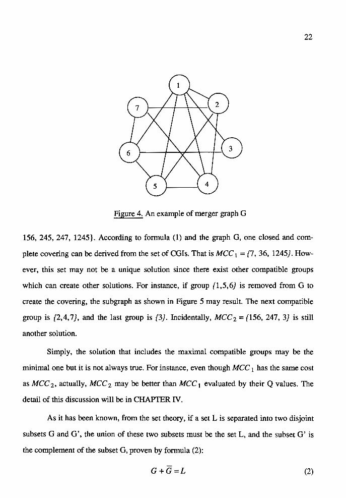
22
Figure 4. An example of merger graph G
156, 245, 247, 1245}. According to formula (1) and the graph G, one closed and com
plete covering can be derived from the set of CGis. That is MCC 1 = {7, 36, 1245). How
ever, this set may not be a unique solution since there exist other compatible groups
which can create other solutions. For instance, if group {l,5,6} is removed from G to
create the covering, the subgraph as shown in Figure 5 may result. The next compatible
group is {2,4,7), and the last group is {3}. Incidentally, MCC2 = {156, 247, 3) is still
another solution.
Simply, the solution that includes the maximal compatible groups may be the
minimal one but it is not always true. For instance, even though MCC 1 has the same cost
as MCC 2. actually, MCC 2 may be better than MCC 1 evaluated by their Q values. The
detail of this discussion will be in CHAPTER IV.
As it has been known, from the set theory, if a set L is separated into two disjoint
subsets G and G', the union of these two subsets must be the set L, and the subset G' is
the complement of the subset G, proven by formula (2):
G+G=L (2)

23
8
Figure 5. Reduced merger graph from Figure 4
As a result, G' must be G.
For achieving the same task as above, the complement graph G can also be
applied. G has to be separated into some complete cliques of incompatible groups. The
disconnected nodes can be colored together for this purpose. The following rules are for
creating a complete covering by using the complement graph G:
(1) Put all the input or PS decimal numbers into the nodes.
(2) Connect all the pairs of nodes which are NOT compatible.
(3) Give any one node a certain color first, supposing that it is 'a'. Then, con
sider the next adjacent node. If it is connected with the first node, give this
node a different color 'b'. Otherwise, color it 'a'. The other nodes should
be compared with all the previous colored nodes in the same way.
(4) The nodes which have no connection with any others will be randomly
given the same color with those colored groups respectively.
(5) Separate the entire graph into various subgraphes according to their
colors. The connections between the nodes which belong to different
subgraphes will no longer be retained. The number of the colors become

24
the number of compatible groups in a solution set. Therefore, the solution
is better when fewer colors are used.
According to these rules, the number of compatible groups included in a complete
covering set is the same as the number of colors used in the merger graph. The nodes
which have the same color belong to the same group.
Figure 6. Complement merger graph from Figure 4
As an example, shown in the complement graph G of graph G from Figure 6, the
nodes which are NOT connected have been arranged in the same group. in this example,
step (1) has been executed, and step (2) starts from node '1' (this is not necessary, other
nodes can also be a starting node), node '2' would have the same color as '1' but not as
'3'. Step (4) is passed because there is not any node which has no connection with any
other node. By the way, the same solutions can also be created by coloring the comple
ment merger graph G as by graph G. In this way, the complement merger graph is
colored as in Figure 7. The same result MCC 1 = {7, 36, 1245) as the one from the graph
G can also be created.
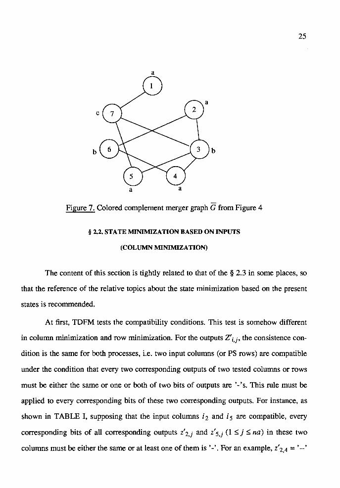
a
b b
a a
Figure 7. Colored complement merger graph G from Figure 4
§ 2.2. STA TE MINIMIZATION BASED ON INPUTS
(COLUMN MINIMIZATION)
25
The content of this section is tightly related to that of the § 2.3 in some places, so
that the reference of the relative topics about the state minimization based on the present
states is recommended.
At first, TDFM tests the compatibility conditions. This test is somehow different
in column minimization and row minimization. For the outputs Z'i,j• the consistence con
dition is the same for both processes, i.e. two input columns (or PS rows) are compatible
under the condition that every two corresponding outputs of two tested columns or rows
must be either the same or one or both of two bits of outputs are ' - 's. This rule must be
applied to every corresponding bits of these two corresponding outputs. For instance, as
shown in TABLE I, supposing that the input columns i1 and i5 are compatible, every
corresponding bits of all corresponding outputs z' 2,j and z' 5,j ( 1 ~ j ~ na) in these two
columns must be either the same or at least one of them is ' -'. For an example, z' 2,4 = ' -- '
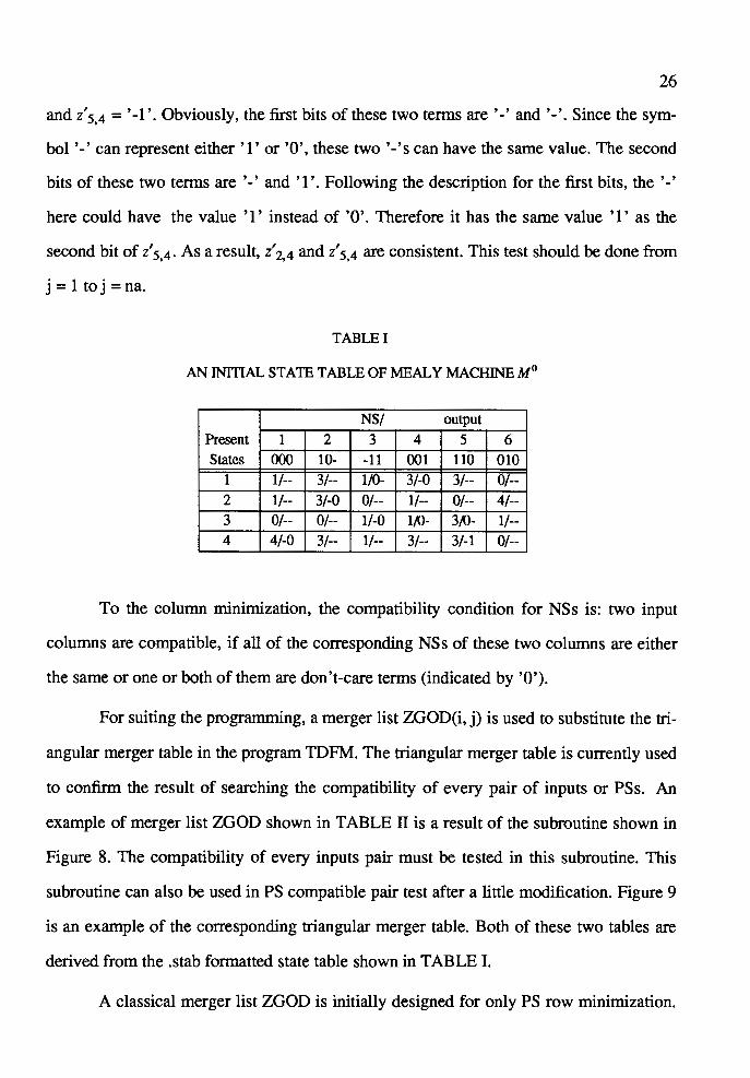
26
and z'5,4 = '-1'. Obviously, the first bits of these two terms are'-' and'-'. Since the sym-
bol ' - ' can represent either '1' or 'O', these two ' - 's can have the same value. The second
bits of these two terms are ' - ' and '1 '. Following the description for the first bits, the ' -'
here could have the value '1' instead of 'O'. Therefore it has the same value '1' as the
second bit of z' 5,4. As a result, z' 2,4 and z' 5,4 are consistent. This test should be done from
j = 1 toj = na.
TABLE I
AN INITIAL STATE TABLE OF MEALY MACHINE M 0
NS/ output
Present 1 2 3 4 5 6 States ()()() 10- -11 001 110 010
1 1/-- 3/-- 1/0- 3/-0 3/-- 0/--2 1/-- 3/-0 0/-- 1/-- 0/-- 4/--3 0/-- 0/-- 1/-0 1/0- 3/0- 1/--4 4/-0 3/-- 1/-- 3/-- 3/-1 0/--
To the column minimization, the compatibility condition for NSs is: two input
columns are compatible, if all of the corresponding NSs of these two columns are either
the same or one or both of them are don't-care terms (indicated by '0').
For suiting the programming, a merger list ZGOD(i, j) is used to substitute the tri
angular merger table in the program TDFM. The triangular merger table is currently used
to confirm the result of searching the compatibility of every pair of inputs or PSs. An
example of merger list ZGOD shown in TABLE II is a result of the subroutine shown in
Figure 8. The compatibility of every inputs pair must be tested in this subroutine. This
subroutine can also be used in PS compatible pair test after a little modification. Figure 9
is an example of the corresponding triangular merger table. Both of these two tables are
derived from the .stab formatted state table shown in TABLE I.
A classical merger list ZGOD is initially designed for only PS row minimization.
27
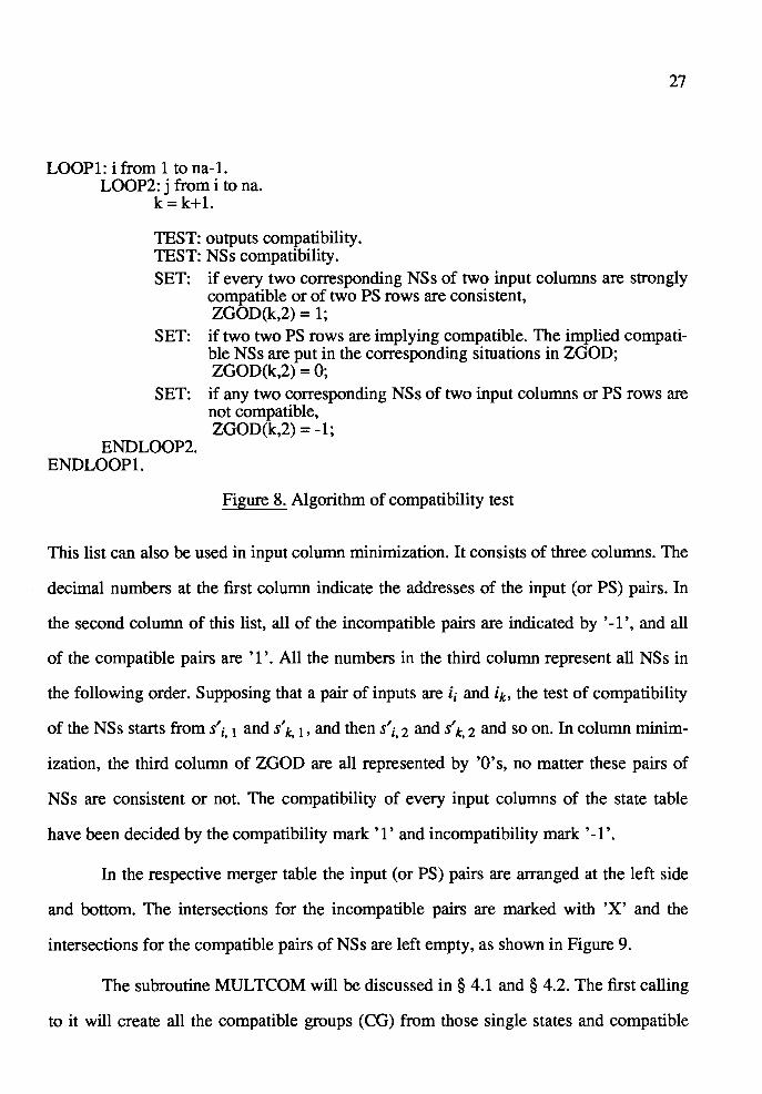
LOOPl: i from 1 to na-1. LOOP2: j from i to na.
k = k+l.
TEST: outputs compatibility. TEST: NSs compatibility. SET: if every two corresponding NSs of two input columns are strongly
compatible or of two PS rows are consistent, ZGOD(k,2) = 1;
SET: if two two PS rows are implying compatible. The implied compatible NSs are put in the corresponding situations in ZGOD; ZGOD(k,2) = O;
SET: if any two corresponding NSs of two input columns or PS rows are not compatible, ZGOD(k,2) = -1;
ENDLOOP2. END LOO Pl.
Figure 8. Algorithm of compatibility test
This list can also be used in input column minimization. It consists of three columns. The
decimal numbers at the first column indicate the addresses of the input (or PS) pairs. In
the second column of this list, all of the incompatible pairs are indicated by '-1 ', and all
of the compatible pairs are '1 '. All the numbers in the third column represent all NSs in
the following order. Supposing that a pair of inputs are ii and it. the test of compatibility
of the NSs starts from s'i, 1 and s' k, l • and then s'i, 2 and s' k, 2 and so on. In column minim-
ization, the third column of ZGOD are all represented by 'O's, no matter these pairs of
NSs are consistent or not. The compatibility of every input columns of the state table
have been decided by the compatibility mark '1' and incompatibility mark '-1 '.
In the respective merger table the input (or PS) pairs are arranged at the left side
and bottom. The intersections for the incompatible pairs are marked with 'X' and the
intersections for the compatible pairs of NSs are left empty, as shown in Figure 9.
The subroutine MULTCOM will be discussed in § 4.1 and § 4.2. The first calling
to it will create all the compatible groups (CG) from those single states and compatible
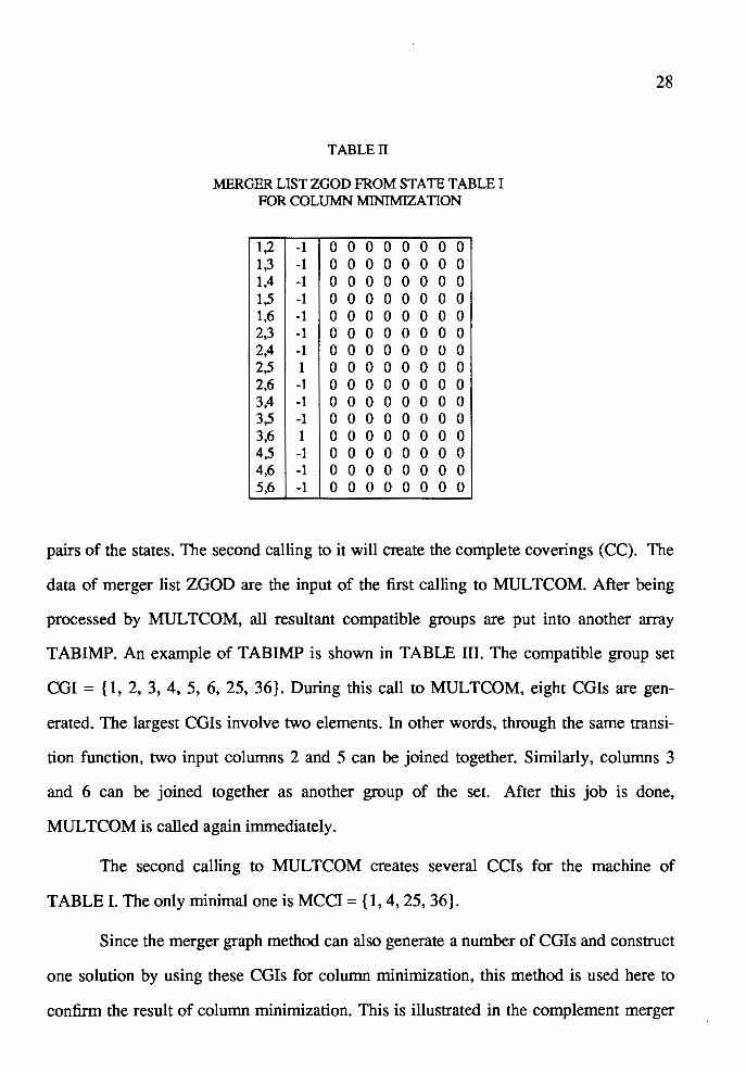
TABLE II
MERGER LIST ZGOD FROM STATE TABLE I FOR COLUMN MINIMIZATION
1,2 -1 0 0 0 0 0 0 0 0 1,3 -1 0 0 0 0 0 0 0 0 1,4 -1 0 0 0 0 0 0 0 0 1,5 -1 0 0 0 0 0 0 0 0 1,6 -1 0 0 0 0 0 0 0 0 2,3 -1 0 0 0 0 0 0 0 0 2,4 -1 0 0 0 0 0 0 0 0 2,5 1 0 0 0 0 0 0 0 0 2,6 -1 0 0 0 0 0 0 0 0 3,4 -1 0 0 0 0 0 0 0 0 3,5 -1 0 0 0 0 0 0 0 0 3,6 1 0 0 0 0 0 0 0 0 4,5 -1 0 0 0 0 0 0 0 0 4,6 -1 0 0 0 0 0 0 0 0 5,6 -1 0 0 0 0 0 0 0 0
28
pairs of the states. The second calling to it will create the complete coverings (CC). The
data of merger list ZGOD are the input of the first calling to MUL TCOM. After being
processed by MUL TCOM, all resultant compatible groups are put into another array
T ABIMP. An example of TABIMP is shown in TABLE III. The compatible group set
CGI = {1, 2, 3, 4, 5, 6, 25, 36}. During this call to MULTCOM, eight CGis are gen-
erated. The largest CGis involve two elements. In other words, through the same transi-
tion function, two input columns 2 and 5 can be joined together. Similarly, columns 3
and 6 can be joined together as another group of the set. After this job is done,
MULTCOM is called again immediately.
The second calling to MUL TCOM creates several CCis for the machine of
TABLE I. The only minimal one is MCCI = { 1, 4, 25, 36}.
Since the merger graph method can also generate a number of CGis and construct
one solution by using these CGis for column minimization, this method is used here to
confirm the result of column minimization. This is illustrated in the complement merger
29
2
3
4
5
6
1 2 3 4 5
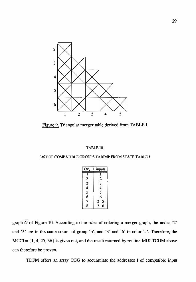
Figure 9. Triangular merger table derived from TABLE I
TABLE III
LIST OF COMPATIBLE GROUPS TABIMP FROM STATE TABLE I
OPi inputs
1 1 2 2 3 3 4 4 5 5 6 6 7 2 5 8 3 6
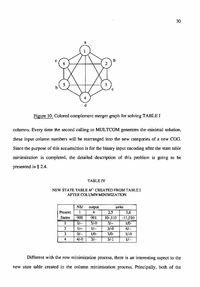
graph G of Figure 10. According to the rules of coloring a merger graph, the nodes '2'
and '5' are in the same color of group 'b', and '3' and '6' in color 'c'. Therefore, the
MCCI = { 1, 4, 25, 36} is given out, and the result returned by routine MULTCOM above
can therefore be proven.
TDFM offers an array CGG to accumulate the addresses I of compatible input
30
a
c b
b
d
Figure 10. Colored complement merger graph for solving TABLE I
columns. Every time the second calling to MUL TCOM generates the minimal solution,
these input column numbers will be rearranged into the new categories of a new CGG.
Since the purpose of this accumultion is for the binary input encoding after the state table
minimization is completed, the detailed description of this problem is going to be
presented in§ 2.4.
TABLEN
NEW STATE TABLE M 1 CREATED FROM TABLE I AFIER COLUMN MINIMIZATION
NS/ output units
Present 1 4 2,5 3,6 States ()()() 001 10-,110 -11,010
1 1/-- 3/-0 3/-- 1/0-2 1/-- 1/-- 3/-0 4/--3 0/-- 1/0- 3/0- 1/-0 4 4/-0 3/-- 3/-1 1/--
Different with the row minimization process, there is an interesting aspect to the
new state table created in the column minimization process. Principally, both of the
31
NS/out units in the corresponding locations of two certain columns are not related to the
input addresses. Therefore, every pair of corresponding NSs of a CGI is consistent, i.e.
their decimal expressions have the same value or the NS don't-care expressions by 'O',
and every corresponding bits of the corresponding outputs of a CGI have also either the
same symbolic expressions or don't-care expressions represented by ' - '. A new symbolic
system is not needed to identify the NSs and the outputs but simply the present number
expressions can still be used. For instance, in TABLE I, NS/output unit { s' I z') ~. 2 = 3 /-0
and (s' !z')~ 2 = 0/-. Therefore, the NS/output units in the second column and the fifth . column of the old table M 0 become one new column. It is the third column of the new
table M 1 of TABLE N, and the NS/output unit in this respective location is
(s' lz'Jl2=3!-0.
§ 2.3 ST ATE MINIMIZATION BASED ON INTERNAL ST ATES
(ROW MINIMIZATION)
After the column minimization, the new state table M 1 is created. Now the task is
to execute the row minimization. Referring to § 2.2, some steps are the same or similar in
both of these procedures, so that the description of row minimization will become some
what simpler. Repetition of the same issues will be avoided, but some of the similar
topics will still be described briefly.
The same as the process of the column minimization, the first step for row minim-
ization is also the test of compatibility conditions. The array ZGOD from TABLE V con
tains all the PS pairs, derived directly from the the state table TABLE N, the result of
the column minimization. If two PS rows satisfy definition ( 1 ), that is, if each pair of the
corresponding outputs (z'i,j• z'k,j} of the pair of PS rows {si, sk] are consistent, i.e.
z' i,j = z' k,j, and every pair of the corresponding next states of these two rows { s' i,j, s' k)
is either consistent, s' i,j = s' k,j, or belongs to their parent states s i or s k, this pair of two
32
rows
{si> s,J is strongly compatible (non- conditionally compatible). Such a group of PS rows
is a strongly compatible group (SCGP). Comparing with the column minimization, the
compatible conditions of row minimization are less strict. Otherwise, according to
definition (3), if some NSs of these two rows belong to some other pairs of the strongly
compatible present states, i.e. { s' i,j, s' k,j} c {Sp, sq}, and others satisfy the requirement of
strongly compatibility, the pair of these two rows {si,s,J which involves (s'i,j·s' k,j} is
called a implying compatible according to definition (3). Such a group of PS rows is an
implying compatible group (ICGP). Implying compatible is also called weakly compati
ble. Another case is: if some pairs of the next states (s'i,j• s' k,j} of a pair of PS {si,s,J is
included in another incompatible state pair {sp, sq}, the pair of PSs, {si,s,J is weakly
incompatible. The last case is: if some corresponding bits of the outputs {z'i,j• z'k,j} of
two PS rows {si, s,J are inconsistent (the corresponding bits of these two outputs are '1'
and '0') the PS pair {si>s,J is strongly incompatible.
The same algorithm as in Figure 8 can be used in the compatibility test. The
merger list ZGOD shown in TABLE V illustrates the result of this test. In the second
column of TABLE V, the strongly compatible pairs are marked by '1 '. The weakly com
patible pairs are marked by 'O'. Both the weakly and the strongly incompatible pairs are
marked by '-1 '. In the third column of ZGOD, if there exists any pair of positive
numbers in a certain row of this column, they are the NSs that is implied by the PSs of
the same row. Therefore, ZGOD has to check the compatibility of another PS pair which
this NS pair are included. If that PS pair is not compatible, the implying compatible mark
'O' of this implying PS pair should be changed to '-1 '.
The implying compatible present state rows can be chosen as the CGPs of a solu
tion in row minimization if the solution that includes such ICGPs satisfy the closure con
dition. The 'O's in the second column of TABLE V are the implying compatible marks

33
for closure test and such NSs are reserved in the third column of ZGOD for the reference
instead of being blocked by 'O's.
Another case is that all the NS pairs are not implied by any PS pair. These NSs
are not necessary to be kept in the third column, no matter whether they are compatible
or not. These sort of NSs are denoted by 'O's in the third column of ZGOD.
TABLEV
MERGER LIST ZGOD CREATED FROM TABLE IV FOR ROW MINIMIZATION
1,2 0 0 0 1 3 0 0 1 4 1,3 1 0 0 0 0 0 0 0 0 1,4 1 0 0 0 0 0 0 0 0 2,3 0 0 0 0 0 0 0 1 4 2,4 -1 1 4 1 3 0 0 1 4 3,4 0 0 0 1 3 0 0 0 0
The following steps are executed for row minimization:
(1) Call to MULTCOM for creating all the CGPs and ICGPS which are listed
in TABLE VI,
(2) Call to MUL TCOM again for creating the closed and complete coverings
for PS rows (CCP). The input data of MULTCOM at this time are: aside
the array TAB IMP, another array SMAX is set for collecting all the clo
sure conditions. One can find the theory and the formulas for the close and
complete covering in CHAPTER I, definitions (5), (6) and (7) of
CHAPTER II, and also in CHAPTER IV.
Above procedure applied to TABLE IV creates two solutions CCP 1 = { 134, 2}
and CCP 2 = { 14, 23} after the second calling to MULTCOM. Both of these two solu
tions are MCCPs. In this particular example, both the solution MCCP 1 and MCCP 2 have
the same cost (the cost value of a solution depends on the number of CGPs and ICGPs

34
TABLE VI
LIST OF COMPATIBLE GROUPS FROM STATE TABLE IV
OP; PSs
1 1 2 2 3 3 4 4 5 1 2 6 1 3 7 1 4 8 2 3 9 3 4 10 1 2 3 11 1 3 4
that a solution set includes. Obviously, the less their number is, the better the solution is).
In the tree search of MUL TCOM, MCCP 2 is created later than MCCP 1, and there is no
further solution which has lower cost and its compatible groups have higher qualities. To
shorten the execution time of searching for the solutions, the routine MUL TCOM is lim
ited to generate only the last found minimal solution. Therefore, the last created solution
MCCP 2 = { 14, 23} is acceptable, and the new state table M 2 with new internal states is
generated.
TABLE VII
NEW STATE TABLE M 2 CREATED FROM TABLE IV AFTER ROW MINIMIZATION
NS/ output units
Present 1 4 2,5 3,6
States ()()() 001 10-,110 -11,010 1 1/-0 2/-0 2/-1 1/0-2 1/-- 1/0- 2/00 1/-0
The way of arranging the new PSs and NSs in a new state table is: since the new
35
table includes two PS rows that covers those four PS rows in the old table, the S 2 s of the
new table are marked {1]2 = {1,4)0 and r2J2 = {2,3) 0 . Therefore, each intersection of
S'2s must belong to either {1]2 or {2]2. Simply, {1]2 = (1,4)0 and {2]2 = {2,3)0 are illus
trated in the respective positions of the new state table M2 (TABLE VII).
Consequently, the outputs of the new table are formed using the same method as
for those in the column minimization. It is performed as follows: the compatibilities of
all corresponding outputs are compared bit after bit. If an output bit is ' -', it must be sub
ject to the value of its corresponding bit of another output. In the case where all those
corresponding bits are ' -'s, they will be retained in the new table.
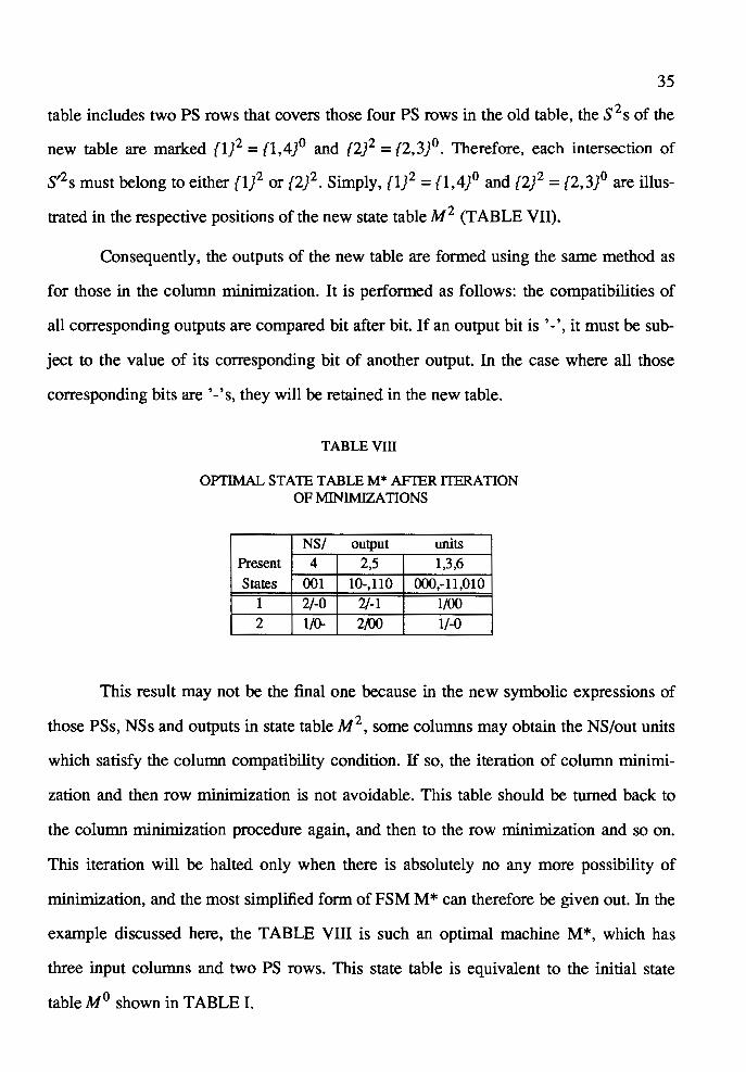
TABLE VIII
OPTIMAL STATE TABLE M* AFIER ITERATION OF MINIMIZATIONS
NS/ output units
Present 4 2,5 1,3,6
States 001 10-,110 000,-11,010
1 2/-0 2/-1 1/00 2 1/0- 2/00 1/-0
This result may not be the final one because in the new symbolic expressions of
those PSs, NSs and outputs in state table M2 , some columns may obtain the NS/out units
which satisfy the column compatibility condition. If so, the iteration of column minimi
zation and then row minimization is not avoidable. This table should be turned back to
the column minimization procedure again, and then to the row minimization and so on.
This iteration will be halted only when there is absolutely no any more possibility of
minimization, and the most simplified form of FSM M* can therefore be given out. In the
example discussed here, the TABLE VIII is such an optimal machine M*, which has
three input columns and two PS rows. This state table is equivalent to the initial state
table M0 shown in TABLE I.
36
§ 2.4 INPUT SIGNAL COMBINATIONAL ENCODING
Following the description in § 2.2, the compatible inputs are accumulated in some
groups. Functionally, these grouped input addresses indicate the input symbolic min
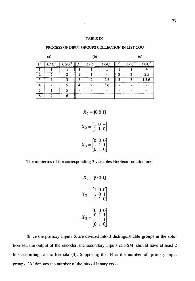
terms. The example of this accumulation is illustrated in TABLE IX. The inputs indi
cated by decimal addresses shown in the headings of TABLE I, TABLE IV and TABLE
VIII are set in different categories. TABLE IX( a) of COG lists every original inputs in
each category. Every time, when a column minimization process is finished, the input
addresses will be distributed in new categories in COG according to the solution set. For
instance, it is found that the binary inputs I~ and Ig are compatible after the first time of
column minimization process, so that the binary inputs I~ and Ig are rearranged in a new
address Ia shown in TABLE IX(b). The number of the inputs in this group, CARD(3, 6)
= 2 is placed in array CFC a. For the same reason, Ig and Ig are arranged in address I~.
Later on, after the second time execution of column minimization, another new input sys
tem is generated and indicated by the address I* in TABLE IX( c ). The input addresses I l and Ia belong to a CGI. The content of CGGl and CGG.l are accumulated into another
new group in address I; of TABLE IX(c). This example illustrates that this accumula
tion process is called by the input decimal addresses I instead of the input binary vari
ables X. Generally, after each execution of column minimization process, all the original
compatible input columns should be collected into one group. When the iterative
machine minimization processes are entirely finished, those groups of inputs will be dealt
with in the input signal encoding procedure.
Reviewing the OMCC created by several column minimization processes, a final
COG, after two column minimization processes, is CGG * = { 4, 25, 136}.
For the combinational logic synthesis, the binary input symbolic expressions are
actually the products of literals (cubes).
37
TABLE IX
PROCESS OF INPUT GROUPS COLLECTION IN LIST CGG
(a) (b) (c)
JU CFCU CGGU 11 CFC 1 CGG 1 r CFC° CGG* 1 1 1 1 1 1 1 1 4 2 1 2 2 1 4 2 2 2,5 3 1 3 3 2 2,5 3 3 1,3,6
4 1 5 4 2 3,6 - - -5 1 5 - - - - - -6 1 6 - - - - - -
x 1=[00 1]
[1 0 -J X2 = 1 1 0
[O 0 OJ X3 = - 1 1 0 1 0
The minterms of the corresponding 3 variables Boolean function are:
x 1=[00 l]
[1 0 OJ X2 = 1 0 1 1 1 0
[o o o] 0 1 1
X 3 = 1 1 1 0 1 0
Since the primary inputs X are divided into 3 distinguishable groups in the solu
tion set, the output of the encoder, the secondary inputs of FSM, should have at least 2
bits according to the formula (3). Supposing that B is the number of primary input
groups, 'A' denotes the number of the bits of binary code.
38
{
ftx(log2B) if MOD(log2 B) = 0
A= jix(log2B) + 1 if MOD(log2 B) > 0 (3)
This encoding could use any kind of code. Since the binary code yields less 'l's
which can simplify the structure of Boolean function and the process of Boolean reduc
tion, TDFM has chosen a ten bits of binary standard code and the code table is stored in
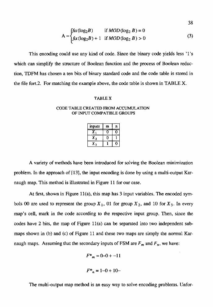
the file fort.2. For matching the example above, the code table is shown in TABLE X.
TABLEX
CODE TABLE CREATED FROM ACCUMULATION OF INPUT COMPATIBLE GROUPS
inputs m n
X1 0 0
Xz 0 1
X3 1 0
A variety of methods have been introduced for solving the Boolean minimization
problem. In the approach of [13], the input encoding is done by using a multi-output Kar
naugh map. This method is illustrated in Figure 11 for our case.
At first, shown in Figure 1 l(a), this map has 3 input variables. The encoded sym
bols 00 are used to represent the group X 1 , 01 for group X 2 , and 10 for X 3 . In every
map's cell, mark in the code according to the respective input group. Then, since the
codes have 2 bits, the map of Figure 11 (a) can be separated into two independent sub
maps shown in (b) and (c) of Figure 11 and these two maps are simply the normal Kar
naugh maps. Assuming that the secondary inputs of FSM are Fm and F n' we have:
F*m = 0-0 +-11
F*n = 1-0 + 10-
The multi-output map method is an easy way to solve encoding problems. Unfor-
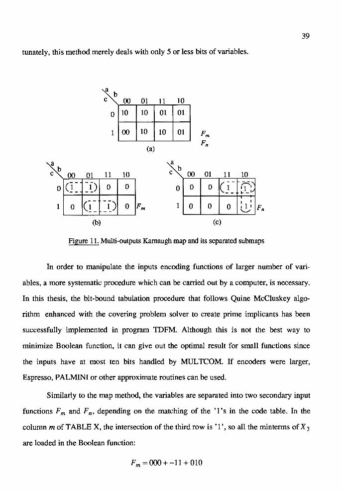
tunately, this method merely deals with only 5 or less bits of variables.
~~ ~A
10 10
()() 10
(a)
vv V.L ~ ~ A~
I (} = =[) 0 0
0 C!~ ~~) 0 Fm
(b)
~~
01
10
A~
01
01
a
Fm Fn
~ ()() 01 11 10
o I o I O I( J ~ f ~: ,..... I I
1 I 0 I 0 I 0 I 0..-' IF n
(c)
Figure 11. Multi-outputs Kamaugh map and its separated submaps
39
In order to manipulate the inputs encoding functions of larger number of vari
ables, a more systematic procedure which can be carried out by a computer, is necessary.
In this thesis, the bit-bound tabulation procedure that follows Quine McCluskey algo
rithm enhanced with the covering problem solver to create prime implicants has been
successfully implemented in program TDFM. Although this is not the best way to
minimize Boolean function, it can give out the optimal result for small functions since
the inputs have at most ten bits handled by MULTCOM. If encoders were larger,
Espresso, PALMINI or other approximate routines can be used.
Similarly to the map method, the variables are separated into two secondary input
functions Fm and F n, depending on the matching of the ' 1 's in the code table. In the
column m of TABLE X, the intersection of the third row is 'l ', so all the min terms of X 3
are loaded in the Boolean function:
Fm=000+-11+010

40
Similar to Fm• for the column n, only the intersection of the second row is 1. Therefore,
the function is:
Fn = 10-+ 110
If there were more groups, for instance, X 4 was a member of inputs, one more code 11
would be appended in the code table. All the variables in X 4 would also be used since the
column m of this code is also ' 1 '.
The tabulation procedure strictly follows these steps:
( 1) Arrange all min terms in groups, so that all terms which have the same
number of 'l's are in the same group. Start with the least number of '1 's
and continue with groups of increasing numbers of 'l's. The number of
'1 's in a term is called the index of that term.
(2) Compare every term of the lowest index group with each term in the suc
cessive group; whenever possible, combine the two terms being compared
by means of the combining theorem Aa + Aa =A. Repeat this by compar
ing each term in a group of index i with every term in the group of index
i+ 1, until all possible applications of the combining theorem have been
exhausted. Two terms from adjacent groups are combinable if their binary
representation differ by just a single digit in the same position; the com
bined term consists of the original fixed representation, with the different
digit replaced by ' -'.
(3) The terms generated in the last step are now compared in the same
fashion: a new term is generated by combining two terms which differ by
only one '1' and whose dashes are in the same position. The process con
tinues until no further combination is possible. The remaining unchecked
terms constitute the set of prime implicants of the function F.
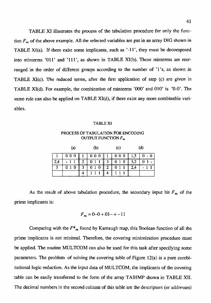
41
TABLE XI illustrates the process of the tabulation procedure for only the func
tion Fm of the above example. All the selected variables are put in an array DIG shown in
TABLE XI( a). If there exist some implicants, such as '-11 ', they must be decomposed
into minterms '011' and '111 ', as shown in TABLE XI(b). These minterms are rear-
ranged in the order of different groups according to the number of ' l's, as shown in
TABLE Xl(c). The reduced terms, after the first application of step (c) are given in
TABLE Xl(d). For example, the combination of minterms '()()()' and 010' is '0-0'. The
same rule can also be applied on TABLE XI(d), if there exist any more combinable vari-
ables.
1 2,4 3
TABLE XI
PROCESS OFT ABULATION FOR ENCODING OUTPUT FUNCTION Fm
(a) (b) (c) (d)
0 0 0 1 0 0 0 1 0 0 0 1,3 0 - 0
- 1 1 2 0 1 1 3 0 1 0 3,2 0 1 -0 1 0 3 0 1 0 2 0 1 1 2,4 - 1 1
4 1 1 1 4 1 1 1
As the result of above tabulation procedure, the secondary input bit Fm of the
prime implicants is:
Fm =0-0+01-+-11
Comparing with the F* m found by Karnaugh map, this Boolean function of all the
prime implicants is not minimal. Therefore, the covering minimization procedure must
be applied. The routine MUL TCOM can also be used for this task after specifying some
parameters. The problem of solving the covering table of Figure 12(a) is a pure combi
national logic reduction. As the input data of MULTCOM, the implicants of the covering
table can be easily transferred to the form of the array TAB IMP shown in TABLE XII.
The decimal numbers in the second column of this table are the descriptors (or addresses)
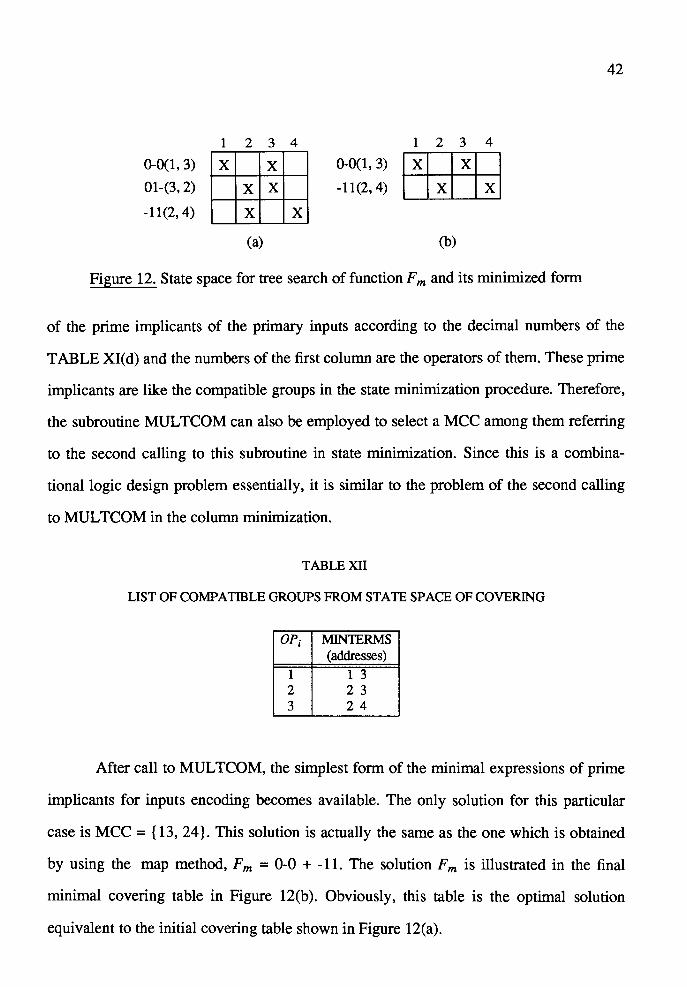
0-0(1, 3)
01-(3, 2)
-11(2, 4)
1
x 2 3 4
x x x x x
(a)
0-0(1, 3)
-11(2, 4)
1 2 3 4
I xi xi xi xi (b)
Figure 12. State space for tree search of function Fm and its minimized form
42
of the prime implicants of the primary inputs according to the decimal numbers of the
TABLE XI( d) and the numbers of the first column are the operators of them. These prime
implicants are like the compatible groups in the state minimization procedure. Therefore,
the subroutine MUL TCOM can also be employed to select a MCC among them referring
to the second calling to this subroutine in state minimization. Since this is a combina-
tional logic design problem essentially, it is similar to the problem of the second calling
to MUL TCOM in the column minimization.
TABLE XII
LIST OF COMPATIBLE GROUPS FROM ST A TE SPACE OF COVERING
OP; MINTERMS (addresses)
1 1 3 2 2 3 3 2 4
After call to MUL TCOM, the simplest form of the minimal expressions of prime
implicants for inputs encoding becomes available. The only solution for this particular
case is MCC = {13, 24}. This solution is actually the same as the one which is obtained
by using the map method, Fm = 0-0 + -11. The solution Fm is illustrated in the final
minimal covering table in Figure 12(b). Obviously, this table is the optimal solution
equivalent to the initial covering table shown in Figure 12(a).

43
Some minimizing possibilities could also result from the state assignment process
to the minimized state table and .kiss formatted data file, but these problems do not
belong to the topic of this thesis.
CHAPTER III
FORMATS OF FINITE STATE MACHINES
The program TDFM can accept two input data formats, .kiss (Keep Internal State
Simple) and .stab (State TABle). Both the .kiss formatted and .stab formatted data are
converted from the standard register-transfer flow chart in format .liss. Presented in Fig
ure 2, two possible conversions that precede the two-dimensional minimization pro
cedure are the machine translation from .liss or .kiss into .stab formatted Mealy machine.
The interconversion of the .kiss and .stab formats is a part of the program TDFM.
The .kiss or .stab data file represents either a completely or an incompletely specified
FSM. The processes of both column and row minimizations are based only on the .stab
formatted Mealy state table. The .kiss formatted file has to be converted into .stab format
before the two-dimensional minimizations (row minimization and column minimization).
On the other hand, the optimal result can also be represented in .kiss or .stab format for
the convenience of next design steps. For instance, some assignment programs, such as
KISS, that was implemented by De Micheli [13] in 1985, prefer to receive the .kiss for
matted data as the input file. Some other programs, such as the programs of CDA system
DIADES, use the .stab formatted file for machine type conversion and assignment.
Although the flow chart conversion process from .liss to .kiss or to .stab is not included in
TDFM, this process is also presented when explaining the forming of a state table. An
example of the flow chart .liss format is shown in Figure 14. This format is quite similar
to the .peg format by [8].
45
§ 3.1. TRANSLATION OF INPUT FILE FORMATS FROM .KISS TO .ST AB
Simply speaking, .kiss format assembles all 4-tuples of parameters into a list. The
parameters in each column are the groups of the external states: the inputs and the out
puts, and the groups of the internal states: the present states and the next states. The fol
lowing notations are presented for .kiss format.
Inputs:
Present states:
Next states:
Outputs:
X = {x1,. .. ,Xmx}
S = {s1,. . .,snaJ
S' = {s'1,1, .. .,s'na,mxJ
' { ' ' } Z= z1.1,. . .,Zna,mx
(4)
(5)
(6)
(7)
Although there exist different types of .kiss format, in this thesis, it is not neces
sary to discuss too much about this topic. One point has to be mentioned, however, that
the reason of using binary symbolic representations for inputs and outputs in the applied
.kiss formatted input file in this thesis is because that the De Micheli's encoding method
for testing of the consistence of the outputs and performing the input combinational
logic encoding has been partly employed as discussed in § 2.4.
A standard .kiss formatted data file is shown in TABLE XIII. For suiting the
usage of this format, the input states are represented in their binary expressions Xi shown
in the first column. The decimal numbers of the second column are internal states and
numbers in the third column are the next state symbols. The binary expressions in the
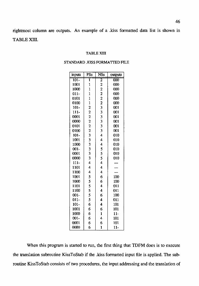
46
rightmost column are outputs. An example of a .kiss formatted data list is shown in
TABLEXID.
TABLE XIII
ST AND ARD .KISS FORMA TIED FILE
inputs PSs NSs outputs
101- 1 2 000 1001 1 2 000 1000 1 2 000 011- 1 2 000 0101 1 2 000 0100 1 2 000 101- 2 3 001 111- 2 3 001 0001 2 3 001 ()()()() 2 3 001 0101 2 3 001 0100 2 3 001 101- 3 4 010 1001 3 4 010 1000 3 4 010 001- 3 5 010 0001 3 5 010 ()()()() 3 5 010 111- 4 4 ---1101 4 4 ---1100 4 4 ---1001 5 6 100 1000 5 6 100 1101 5 4 011 1100 5 4 011 001- 5 6 100 011- 5 4 011 101- 6 4 101 1001 6 6 101 1000 6 1 11-001- 6 4 101 0001 6 6 101 ()()()() 6 1 11-
When this program is started to run, the first thing that TDFM does is to execute
the translation subroutine KissToStab if the .kiss formatted input file is applied. The sub
routine KissToStab consists of two procedures, the input addressing and the translation of

47
formats.
In the standard .kiss formatted file, there is no corresponding decimal addresses I
for inputs. The program has to arrange the decimal addresses for the input binary expres
sions when this .kiss file is read in. This procedure is called the input addressing. Since
the purpose of this addressing for the .kiss formatted file is to arrange the inputs in the
numbers at the headings of state table, the method applied in this process is:
( 1) Enumerate the first term of input with integer 1.
(2) Increase the number when the present binary expression is different with
the expressions already checked above. Otherwise use the same number as
the one which has been assigned to this term. The algorithm of this
arrangement is presented in Figure 13.
TABLE XIV is the result of applying this subroutine. In this input file, the
modified .kiss formatted input file, the decimal numbers have been marked from 1 to 12
inside the parentheses.
If the next state and all bits of output of a NS/output unit are don't-care terms,
such a type of don't-care unit is called complete don't-care unit. The complete don't-care
units are not presented in .kiss formatted input file. When the .kiss format file is
translated into .stab format file, in the corresponding intersections of .stab formatted
input file, this type of NS/output units have to be marked by 'O' for NS and all '-'s for
output. Otherwise, if NS or some bits of the output (not all) of a NS/output unit are
don't-cares, it is called incomplete don't-care unit.
There are two reasons why the decimal numbers of the PSs and inputs should start
from 1. First, in the incompletely specified FSM, more or less don't-care terms in both of
the NSs and outputs are possible. These don't-care terms may be either the complete
don't-care units or the incomplete don't-care units. The complete don't-care units do not
appear in the .kiss formatted file. During the translation, the complete don't-care
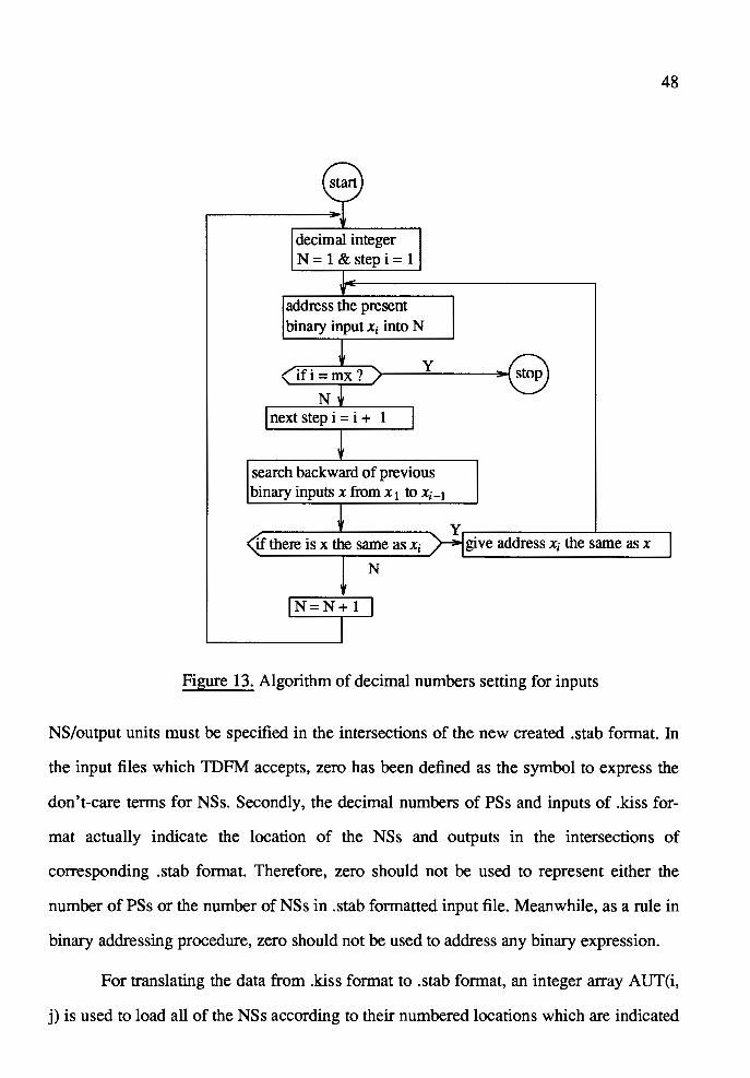
decimal integer N= 1&stepi=1
address the present binary input x; into N
y
N next step i = i + 1
search backward of previous binary inputs x from x 1 to x; _ 1
if there is x the same as x;
N
N=N+ 1
48
Y.----~~~~~~-'-~~~--, give address xi the same as x
Figure 13. Algorithm of decimal numbers setting for inputs
NS/output units must be specified in the intersections of the new created .stab format. In
the input files which TDFM accepts, zero has been defined as the symbol to express the
don't-care terms for NSs. Secondly, the decimal numbers of PSs and inputs of .kiss for
mat actually indicate the location of the NSs and outputs in the intersections of
corresponding .stab format. Therefore, zero should not be used to represent either the
number of PSs or the number of NSs in .stab formatted input file. Meanwhile, as a rule in
binary addressing procedure, zero should not be used to address any binary expression.
For translating the data from .kiss format to .stab format, an integer array AUT(i,
j) is used to load all of the NSs according to their numbered locations which are indicated
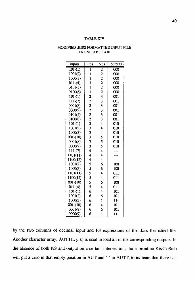
TABLE XIV
MODIFIED .KISS FORMA TIED INPUT FILE FROM TABLE XIII
inputs PSs NSs outputs
101-(1) 1 2 000 1001(2) 1 2 000 1000(3) 1 2 000 011-(4) 1 2 000 0101(5) 1 2 000 0100(6) 1 2 000 101-(1) 2 3 001 111-(7) 2 3 001 0001(8) 2 3 001 0000(9) 2 3 001 0101(5) 2 3 001 0100(6) 2 3 001 101-(1) 3 4 010 1001(2) 3 4 010 1000(3) 3 4 010
001-(10) 3 5 010 0001(8) 3 5 010 0000(9) 3 5 010 111-(7) 4 4 ---
1101(11) 4 4 ---1100(12) 4 4 ---1001(2) 5 6 100 1000(3) 5 6 100 1101(11) 5 4 011 1100(12) 5 4 011 001-(10) 5 6 100 011-(4) 5 4 011 101-(1) 6 4 101 1001(2) 6 6 101 1000(3) 6 1 11-001-(10) 6 4 101 0001(8) 6 6 101 0000(9) 6 1 11-
49
by the two columns of decimal input and PS expressions of the .kiss formatted file.
Another character array, AUTI(i, j, k) is used to load all of the corresponding outputs. In
the absence of both NS and output on a certain intersection, the subroutine KissToStab
will put a zero in that empty position in AUT and'-' in AUTT, to indicate that there is a
50
complete don't-care term in that location.
An example of translating the NSs and outputs from the .kiss formatted input file
into the corresponding .stab formatted file can be illustrated at row 23 of TABLE XIV.
The input number is 3 and the PS's number is 5, so that the NS s\5 = 6 and output
z\5 = 100. These two terms consist of a NS/output unit in the corresponding location of
the .stab format file shown in TABLE XVI.
The .stab formatted file is a two dimensional matrix and the .kiss formatted file is
a list with 4 columns. The decimal numbers marked for inputs of the .kiss formatted file
form the numbers of columns in the corresponding .stab fomatted file. Meanwhile, the
decimal numbers of PSs form the numbers of rows. Therefore, TABLE XVI has 12
columns and 6 rows since the maximal number of addressed inputs is mx = 12 and the
maximal number of PSs is na = 6. According to 'na' and 'mx', the size of .stab input file
can be therefore decided.
§ 3.2. TRANSLATION OF INPUT FILE FORMATS FROM .LISS TO .STAB
According to Figure 2, another possible stage that precedes the state minimization
procedure is the translation from a high level language description of FSM or a state flow
chart (in format .liss) into a .stab formatted Mealy state table directly. An example of
such a flow chart is shown in Figure 14. The description of the translation of this example
will illustrate how a state table of a FSM is formed in this way. In addition, the following
modification of this state table creates a number of complete don't-care terms by using
the invariants. These don't-care terms consequently make more columns and rows of the
modified state table compatible. Referring this example, the data notation are as follows.
( 1) There are six present states in this flow chart. The symbols s 1 to s 6 in the
graph nodes represent these PSs. Therefore, they can be put in the list of
PSs in the state table immediately.
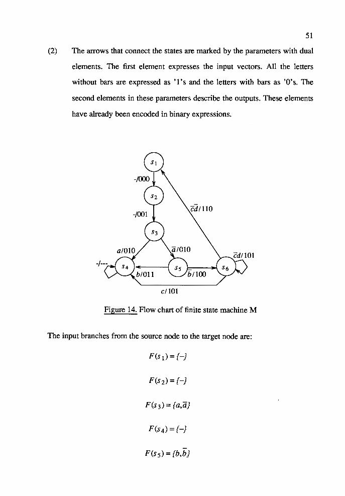
51
(2) The arrows that connect the states are marked by the parameters with dual
elements. The first element expresses the input vectors. All the letters
without bars are expressed as '1 's and the letters with bars as 'O's. The
second elements in these parameters describe the outputs. These elements
have already been encoded in binary expressions.
c/101
Figure 14. Flow chart of finite state machine M
The input branches from the source node to the target node are:
F(s1)={-}
F(s2) = {-}
F(s 3) = {a,a}
F(s4) = {-}
F(s5) = {b,b}
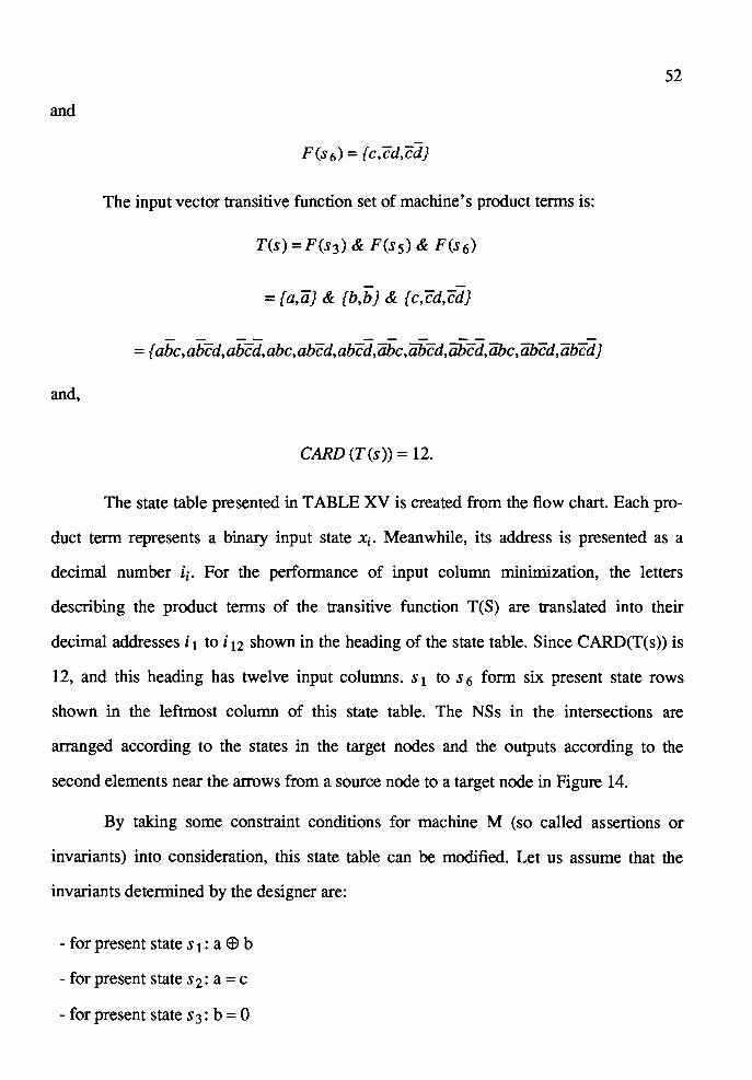
52
and
F(s6) = {c,cd,cdJ
The input vector transitive function set of machine's product terms is:
T(s) =F(s3) & F(ss) & F(s6)
= {a,aJ & {b,bJ & {c,cd,cdJ
- - - -= {abc,abcd,abcd,abc,abcd,abcd,'iibc,abcd,abcd,abc,abcd,abcdJ
and,
CARD (T(s)) = 12.
The state table presented in TABLE XV is created from the flow chart. Each pro-
duct term represents a binary input state Xi. Meanwhile, its address is presented as a
decimal number ii· For the performance of input column minimization, the letters
describing the product terms of the transitive function T(S) are translated into their
decimal addresses i 1 to i 12 shown in the heading of the state table. Since CARD(T(s)) is
12, and this heading has twelve input columns. s 1 to s 6 form six present state rows
shown in the leftmost column of this state table. The NSs in the intersections are
arranged according to the states in the target nodes and the outputs according to the
second elements near the arrows from a source node to a target node in Figure 14.
By talcing some constraint conditions for machine M (so called assertions or
invariants) into consideration, this state table can be modified. Let us assume that the
invariants determined by the designer are:
- for present state s 1 : a E9 b
- for present state s 2: a = c
- for present state s 3 : b = 0
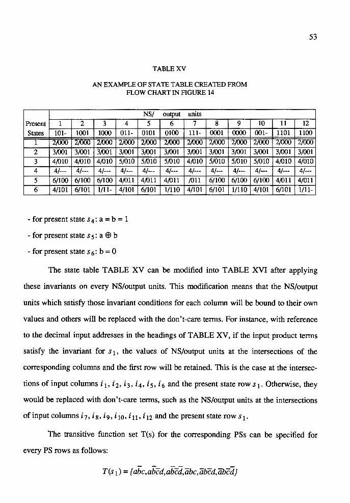
TABLE XV
AN EXAMPLE OF STATE TABLE CREATED FROM FLOW CHART IN FIGURE 14
NS/ output units
Present 1 2 3 4 5 6 7 8 9 States 101- 1001 1000 011- 0101 0100 111- 0001 ()()()()
1 2.iOOO 2/000 2,ooQ 2/000 2/000 2.iOOO 2ft)OO 2/000 2.iOOO
2 3/001 3/001 3/001 3/001 3/001 3/001 3/001 3/001 3/001
3 4/010 4/010 4/010 5/010 5/010 5/010 4/010 5/010 5/010
4 4/--- 4/--- 4/--- 4/--- 4/--- 4/--- 4/--- 4/--- 4/---
5 6/100 6/100 6/100 4/011 4/011 4/011 /011 6/100 6/100
6 4/101 6/101 1/11- 4/101 6/101 1/110 4/101 6/101 1/110
- for present state s 4: a = b = 1
- for present state s 5 : a E9 b
- for present state s 6: b = 0
53
10 11 12
001- 1101 1100
2/000 2.iOOO 2/000
3/001 3/001 3/001
5/010 4/010 4/010
4/--- 4/--- 4/---
6/100 4/011 4/011
4/101 6/101 1/11-
The state table TABLE XV can be modified into TABLE XVI after applying
these invariants on every NS/output units. This modification means that the NS/output
units which satisfy those invariant conditions for each column will be bound to their own
values and others will be replaced with the don't-care terms. For instance, with reference
to the decimal input addresses in the headings of TABLE XV, if the input product terms
satisfy the invariant for s 1 , the values of NS/output units at the intersections of the
corresponding columns and the first row will be retained. This is the case at the intersec
tions of input columns i 1 , i 2, i 3, i 4, i 5, i 6 and the present state row s 1 . Otherwise, they
would be replaced with don't-care terms, such as the NS/output units at the intersections
of input columns i 1, is, i 9, i 10. i 11. i 12 and the present state rows 1 ·
The transitive function set T(s) for the corresponding PSs can be specified for
every PS rows as follows:
- - - - -T(s 1) = { abc, abed, abed, abc, abed, abed}
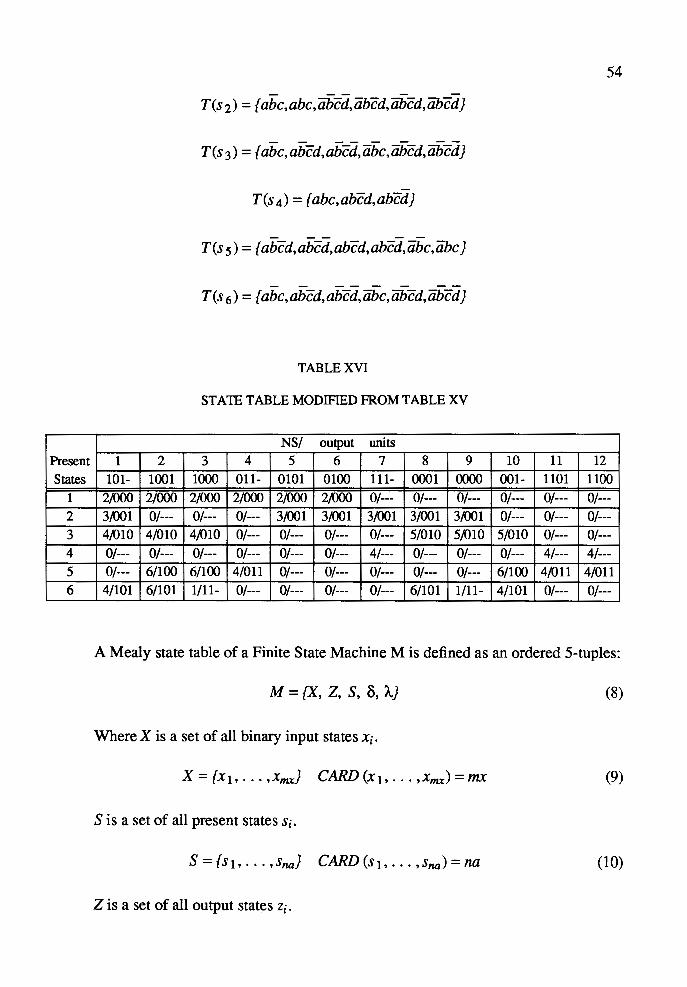
54 - - - - -
T(s 2) = {abc,abc,abcd,abcd,abcd,abcdJ
- - -- - -T(s 3 ) = {abc,abcd,abcd,abc,abcd,abcd}
T(s 4 ) = {abc,abcd,abcd}
T(s 5) = {abcd,abcd,abcd,abcd,abc,abc}
- - -- - -T(s 6 ) = {abc,abcd,abcd,abc,abcd,abcd}
TABLE XVI
STAIB TABLE MODIFIED FROM TABLE XV
NS/ output units
Present 1 2 3 4 5 6 7 8 9 10 11 12
States 101- 1001 1000 011- 0101 0100 111- 0001 ()()()() 001- 1101 1100
1 2/000 2/000 2/000 2/000 2/000 2/000 0/--- 0/--- 0/--- 0/--- 0/--- 0/---2 3/001 0/--- 0/--- 0/--- 3/001 3/001 3/001 3/001 3/001 0/--- 0/--- 0/---
3 4/010 4/010 4/010 0/--- 0/--- 0/--- 0/--- 5/010 5/010 5/010 0/--- 0/---4 0/--- 0/--- 0/--- 0/--- 0/--- 0/--- 4/--- 0/--- 0/--- 0/--- 4/--- 4/---
5 0/--- 6/100 6/100 4/011 0/--- 0/--- 0/--- 0/--- 0/--- 6/100 4/011 4/011 6 4/101 6/101 1/11- 0/--- 0/--- 0/--- 0/--- 6/101 1/11- 4/101 0/--- 0/---
A Mealy state table of a Finite State Machine Mis defined as an ordered 5-tuples:
M = {X, Z, S, B, /...) (8)
Where X is a set of all binary input states xi.
X = {x1, ... ,Xmx} CARD (X1, ... ,Xmx) = mx (9)
Sis a set of all present states Si.
S = {s1, ... ,sna} CARD (s1, ... ,sna) = na (10)
Z is a set of all output states Zi.

Z = { z 1, ... , z,J CARD (z 1 •... , zk) = k
55
(11)
X, S and Z are the basic sets of states of machine M. These three sets of states
determine the size of the machine. () is a two dimensional matrix used to map the succes
sors of PSs, the next states s' related to the inputs. It is the so called next state transition
function X* S -7 S'.
S' = B(Xi.Sj) = (s'i,j} 1 ~ i ~ m.x, 1 ~ j ~ na CARD (s'i,j) = mx * na (12)
A. is another two dimensional matrix used to map the outputs related to the present
states and input states. It is the so called output function X*S-7Z'.
Z' = A.(xi,Sj) = (z'i,j} 1 ~ i ~ m.x, 1 ~ j ~ na CARD (z'i,j) = mx * na (13)
According to the structure of Mealy machine M, the PSs and NSs are internal
states and the inputs and outputs are external states. In the form of the Mealy state table,
these 5-tuple elements are arranged in their individual locations. The PSs Sj (l~j~a) are
in the leftmost column. The inputs Xi (1 ~ i ~ m.x) are in the heading. Each unit of
NS/output { s' I z' hi is located in an intersection of the table. Their addresses j and i are
indicated by PSs Sj and input decimal expressions ii. Obviously, 'na', the number of PSs
also indicates the number of the NS/output units under each input column. So does 'mx',
the number of input states also indicates the number of the NS/output units under each PS
row.
The state table input format is the most popular format for representing FSMs,
because it clearly gives out the relationship of the inputs (represented in the columns of
the state table array) and the internal present and next states (in the rows). State table is
presented in Mealy or Moore model. In this program, the Mealy machine is recom
mended for all minimization procedures. All the definitions presented in § 2.1 are also
based on the state table of Mealy model because it permits to generate the compatible
groups column by column or row by row. The format for representing state tables is
56
called the format .stab. An example of state table of a Mealy machine M is shown in
TABLE XVI. It has twelve columns, which mean the machine has twelve distinguishable
input states and six rows which mean six internal present states s 1' ... ,s 6. The internal
present states shown in the leftmost column of the state table do not need binary sym
bolic expressions because there is no encoding problem at this stage. Each time when the
row minimization is accomplished, a new state numbering system of the state table will
be used to replace the old one. Meanwhile, for performing the state minimization based
on input columns introduced in § 2.2, they are represented by decimal numbers shown in
the input columns at the heading of state table as well as the addresses i 1, ... , i 12. For per
forming the input combinational logic encoding, inputs are marked by binary symbols
XJ, •• .,X12.
TDFM handles multi-bit input and output machines, so that the outputs are also
represented in binary symbols. This is not only for the performance of testing the output
consistence in both column and row minimizations but also for the performance of sym
bolic FSM assignment.
Program TDFM can deal with either completely specified sequential machines or
incompletely specified sequential machines. This means it is possible that some binary
representations or some bits of these binary representations have 'uncertain' values in the
inputs and outputs. In other words, the don't-care terms mean that these bits of the binary
representation may have double values 'l' and 'O'. In the program TDFM, character ' -'
can represent the don't-care term for both inputs and outputs and binary number 'l' or
'O' will represent one certain value. To the next states, 'O' will represent the don't-care
terms and the positive integers will represent the states that have certain specified values.
-------
57
§ 3.3 SPECIFICATION OF INPUT FILES
The TDFM programming utilizes a group of arrays. Some arrays are quite huge,
especially those arrays that have two or three dimensions. Meanwhile, the computers can
offer different sizes of memory spaces for running this program. As a result, the size of
the FSM must be limited. Running on VAX 11 system, the memory space is limited to
2.5mb. The arrays in TDFM for the inputs and present states are both limited to at most
fifty distinguishable expressions if the percentage of don't-care terms is not higher than
about 30% by estimation in both of NSs and outputs. These limits are based on the exper
iment of machine Mb shown in TABLE XIX. Obviously, the present states are
represented from 1 to 50 in order (note this: there is no '0'). As the successors of PSs, the
next states (NS) are limited in the same domain as PSs. The same limits of fifty different
expressions for binary inputs and outputs are also mentioned. Since both of inputs and
outputs are represented by binary symbols, according to the formula (14), 'B' is the
number of binary bits and 'A' will be the numbers of different expressions.
{
]i.x(log2 A) if MOD(log2 A)= 0
B = .fix(log2 A)+ 1 if MOD(log2 A)> 0 (14)
Assuming that A= 50 and there is no don't-care expression'-' in any bit among
those inputs or outputs, at most B = 6 bits of binary expressions are permissible.
The binary expressions which have more than six bits are still possible if there
exist some '-'sin some bits of inputs and outputs, but the total number of them should
not be more than fifty distinguishable expressions. Concentrating on the binary inputs, if
there are some don't-care bits in some binary expressions, any two inputs should not be
contrary. For instance, the input of the fourth column of TABLE XVI, 011- is actually
the combination of the terms 0110 and 0111. Therefore, if this combined term exists in
the list, it is illegal to have its implied term included in anywhere else of the input list.
58
The IDFM program can receive both the .kiss and the .stab input formats. It is,
however, not permissible to change anything in the source file of IDFM system since the
program IDFM is written in FORTRAN. Usually, the FSMs which users want to
minimize may have different formats or sizes. Moreover, different strategies for the
application of subroutines of IDFM are possible in practice. In IDFM system, a group of
data files 'fort' are offered to suit different cases. Fort.1 is for input data specification.
For instance, if the inputs or outputs of several machines have different sizes or different
bits, users can simply change some parameters in these fort files for TDFM's process.
In the example of fort.1 shown in TABLE XVII, the input file has been .kiss for
matted. The character following the term 'formt' denotes the format. The term 'formt' is
modified for dealing with a .kiss formatted input file if the following character is 'k'. The
numbers following the terms 'inbit' (means the bit of input) and 'oubit' (means the bits
of output) must be settled up for .kiss formatted file. The first and the last numbers of the
characters from 'forma' to 'formc' are required to be marked directly corresponding to
the 'inbit' and 'oubit'. For example, the 'inbit' of this table is 4 and the 'oubit' is 3 for
the .kiss formatted file TABLE XIV. The numbers following the terms 'innum' and
'psnum' should be ignored.
To the .stab formatted input file, the file fort. l can also be modified to deal with a
.stab formatted input file if the character following the term 'formt' is 's'. The numbers
following the terms 'oubit', 'innum' (means the number of inputs) and 'psnum' (means
the number of present states) must also be settled up according to the size of the state
table. The characters from 'formd' to 'forme' are required to be marked directly
corresponding to the 'oubit', 'innum' and 'psnum'. Other terms could be ignored in this
setting. The example of this specification for .stab formatted file TABLE XVI is: 'oubit'
equals '3', 'innum' is '12' and 'psnum' is '6'.
As an extra feature, TDFM gives out the percentage of don't-care terms of .stab
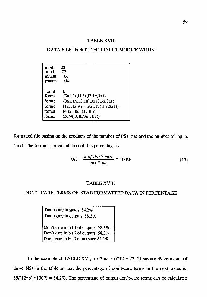
TABLE XVII
DATA FILE 'FORT.1' FOR INPUT MODIFICATION
inbit oubit inn um psnum
formt forma formb formc formd forme
03 03 06 04
k (3al ,3x,i3,3x,i3, lx,3al) (3al, lh(,i3, lh),3x,i3,3x,3al) (lal,lx,3h = ,3al,12(lh+,3al)) (4(i2,lh/,3al,lh )) (20/4(i3,lh/3al,lh ))
59
formatted file basing on the products of the number of PSs (na) and the number of inputs
(mx). The formula for calculation of this percentage is:
#of don't care * 100% DC= mx * na
TABLE XVIII
DON'T CARE TERMS OF .STAB FORMATTED DATA IN PERCENTAGE
Don't care in states: 54.2% Don't care in outputs: 58.3%
Don't care in bit 1 of outputs: 58.3% Don't care in bit 2 of outputs: 58.3% Don't care in bit 3 of outputs: 61.1 %
(15)
In the example of TABLE XVI, mx * na = 6*12 = 72. There are 39 zeros out of
those NSs in the table so that the percentage of don't-care terms in the next states is:
39/(12*6) *100% = 54.2%. The percentage of output don't-care terms can be calculated

~--~--- -----
60
as well. The number of the outputs which have ' -'s on all of 3 bits are 42. As a result, the
percentage of output don't-care terms is 42/(12*6) *100% = 58.3%. The detailed infor
mation of output don't-care percentage are also reported for each output bit separately.
All the don't-care terms in bits 1 and 2 of the outputs are 42 and the don't-care terms for
only bit 3 are 44 so that these percentages are 42/(12*6) *100% = 58.3% and 44/(12*6)
*100% = 61.1 % respectively. In TDFM, KissToStab will calculate these percentages
immediately after the input file is read in. The example of this process printout is shown
in TABLE XVIII.

CHAPTER IV
DESCRIPTION OF ROUTINE MULTCOM
The routine MULTCOM, first introduced by M. Perkowski in 1977 [14] is based
on the theory of Artificial Intelligence. It is used for solving problems which have many
solution sets, and among them, one or more minimal solutions exist. MUL TCOM per
forms a tree search synthesis to arrange the groups of the elements into sets (or the ele
ments into groups) according to the pre-decided conditions and the priority of these
groups (or elements). These conditions are variant in different tasks. For instance, in state
table minimization problems, this subroutine is applied twice. The condition of the first
application is that all the groups must be compatible. The conditions of the second appli
cation are that the compatible groups in a solution set must be closed and complete. The
quality of a compatible group is decided by the number of elements that this group has
covered and also, particularly, the degree of implying internal states of the COP in PS
row minimization or the number of the binary don't-care terms of the CGI in input
column minimization. The set must be minimal under the necessary conditions of the
closure and completeness. Such a solution set has a minimum cost. A set which has the
minimum cost and all of its CGs have the higher qualities will be the minimal solution.
§ 4.1. SELECTION OF STRATEGIES, PARAMETERS AND SIZE LIMITATION OF TREE
The subroutine MULTCOM's experience comes from the learning and anticipa
tion abilities. Learning means that every time the MUL TCOM creates a new node, the
routine will compare this node with all its parent nodes. If this node has a higher quality
value, it will be kept for the further extension; otherwise, it will not be kept. Anticipation
62
means that every time before MULTCOM creates a new node, it will look ahead to deter
mine if this new created node will lead to a minimal solution or not. If it does, this node
will be created; otherwise, this creation will be aborted. Generally, these learning and
anticipation abilities are based on the calculation and comparison of the quality functions
of the current applied node and its parent nodes. A number of heuristic, in other words,
trial-and-error processes is actually unavoidable; and so far, for speeding up the algo
rithm, the routine offers a number of search strategies for different tasks:
(1) Breadth First: with this strategy, each newly created node is appended to
the end of the 'open-list' which contains all the nodes waiting for the
extension. Each time the first node in the list is selected for this extension,
it is removed from this list. After all the available operators for this node
have been applied, the extension backtracks to another branch in the
open-list.
(2) Depth First: this is a strategy to extend the most recently generated node
first. Until it reaches a certain specified depth limit (defined by users), the
search backtracks to extend another node which is the deepest but does
not exceed this depth limit. The newly created node is put at the beginning
of the list so that the first node in this list is always the deepest one.
(3) Branch and Bound: with this strategy, a cost function CF(N) calculated by
routine FOC(N) is defined for each candidate node, where N is the node's
number of a solution set. A desired cost value F has been set before the
tree searching started and it holds the minimum cost of the solution
already found. Whenever a new node is generated, the cost value of the
solution set is compared with the value F. All the solutions whose costs
are larger than F will be cut-off from the tree.
(4) Ordering: This strategy can be selected in cooperation with the branch and

63
bound strategy. For this strategy, a quality function Q(op) is defined to
evaluate the cost function CF(N) for all operators (op) of the node under
extension. The order of application of these operators is in accordance
with their evaluated qualities. Actually, the node which has the highest
value Q will be arranged to have the priority to be chosen for the present
extension.
Meanwhile, the successive application of this subroutine also depends upon the
variant properties of a particular problem. For instance, the satisfaction of the complete
ness condition and the closure condition for the set of compatible states must be tested in
some cases. The time of generating solutions depends on the selection of the strategies
because the behavior of the algorithm is strongly parameter-dependent. For instance, the
Breadth First strategy can quickly create all solutions without checking their cost values
and qualities of the compatible groups (represented by their operators). In contrast, the
Branch and Bound strategy cooperating with Ordering will create the first minimal solu
tion without searching all nodes. Generally, creating a solution needs much less time than
proving its feasibility. Before the routine is called, the suitable setting of different stra
tegies for different tasks is proposed.
The parameters for MUL TCOM are:
(1) GENAS: This parameter causes the calling of local search procedure GEN
for the indispensable nodes. Lack of it causes only the global search.
(2) PRINT: This parameter causes the printing of descriptions of all states
during the search.
(3) EQUI: This parameter causes the calling to subroutine EQUI for discover
ing the 'included' compatible groups of a solution set. It is used only for
finding the MCC sets.
64
(4) ORD: This parameter causes the calling to subroutine ORD for the Order
ing search strategy.
(5) MUST: This parameter causes the calling to subroutine MUSTO for
finding all indispensable operators for nodes extension in the tree.
(6) SPRA W: This parameter causes that each new node of the tree (also the
solution) is compared with all previously created nodes. If this node has
the same quality as others, it will not be stored in the record of nodes in a
tree (the record array SMAX stores the operators which have the higher
qualities). This parameter is used only for the problem in which the same
states are unavoidable in the search.
(7) MEMO: This parameter causes that the number of all newly created nodes
be appended at the beginning of the list OPEN. Otherwise, they are
appended at the end of the list. Hence, the value of this parameter is
important only in the case of the first element in the list OPEN being
selected (this corresponds to the case when the parameter SELECT equals
0). In practice, when SELECT = 0, MEMO = 0 indicates the Breadth First
search strategy, and MEMO= 1 indicates the Depth First search.
(8) SELECT (values 0,1,2): Value 0 means that the first element in list OPEN
is selected for tree extension. Value 1 means that the "random" node is
selected and a procedure of probability distribution is called for this selec
tion. Value 2 means that the node with maximum value of quality function
(an attempt to find the minimal solution) is selected.
Some data are set for the specification of the tree size:
(1) NCMAX: Maximal number of the nodes extended. Standard value is
1000.

65
(2) SDMAX: Maximal depth of nodes in the tree for Depth First strategy.
Standard value is 20.
The parameters and the data listed above are set only for solving the problems
described in this paper. We will not discuss those unnecessary parameters and data. For
the same reason, in this section, all the discussions are also limited to state minimization
and minimal covering problem (the input encoding) which are related to just the content
of this thesis.
The routine MUL TCOM is called by TDFM for completing three different tasks,
the column minimization, the row minimization and the input encoding. In both column
and row minimization, MULTCOM is called twice. The first calling in both column and
row minimizations is for the creation of all compatible groups. The input of this calling is
the merger list ZGOD and the output is the compatible groups list TABIMP. The second
calling to MUL TCOM is for the creation of the minimal closed and complete coverings.
The input of this calling is the compatible groups list TAB IMP and the output is the
newly created state table. There is no difference in setting the parameters and data for
both column and row minimization procedures in the first calling to MUL TCOM. In the
second calling, the closed and complete conditions must be checked in the second calling
in row minimization. On the other hand, the checking of closure can be waived in the
second calling in column minimization.
Before running MUL TCOM, some preparations must be mentioned. Besides the
array ZGOD or TABIMP, some other arrays and declarators are needed for these
processes. Even though the purpose of these arrays and a variety of the declarators may
vary in different tasks, basically, they have a uniform usage. The notation will help us to
understand the verbal description of the tree search.
The arrays:

66
(1) RS : The auxiliary set of the operators that are NOT applied in the tree.
(2) AS : The set of closure conditions for every compatible pair in group QS.
(3) QS : The set of states in a compatible group corresponding to the respec
tive node.
(4) GS: Set of all operators which can be applied in node NC.
and the declarators:
(1) NC : Nodes number.
(2) SD : The depth of the nodes in the tree.
(3) PC : The number of the direct predecessor.
(4) OP: The number of the operators from PC to NC.
(5) CF: The cost function value.
§ 4.2. CALLING TO MULTCOM FOR FINDING ALL COMPATIBLE GROUPS
This calling to MUL TCOM is to create all compatible groups. The strategy for
defining those parameters is relatively simpler because MUL TCOM is needed only to list
all the compatible groups (implicants). There is not the feasibility problem for creating
the compatible groups. In other words, in this case, there is no cost function for the node
and no quality function for the operator. The results must satisfy only the compatible
conditions which have been indicated in the list ZGOD.
The strategy of Breadth First is chosen for this task because all the nodes on this
tree have to be appended and then the compatibilities among the compatible pairs have to
be checked. In particular, parameters MEMO = 0 and SELECT = 0 are necessary. In
order to speed up this extension, subroutine GEN is used to check the compatibility of
the operators appended on a certain node. Therefore, the parameter GENAS = 1 must be
established. These parameters are set in the data file 'fort.3'.
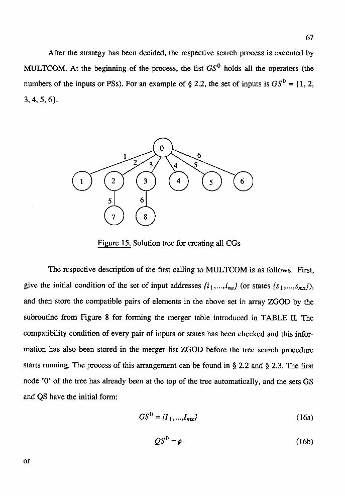
67
After the strategy has been decided, the respective search process is executed by
MULTCOM. At the beginning of the process, the list GS 0 holds all the operators (the
numbers of the inputs or PSs). For an example of§ 2.2, the set of inputs is GS0 = { 1, 2,
3, 4, 5, 6}.
8
Figure 15. Solution tree for creating all CGs
The respective description of the first calling to MUL TCOM is as follows. First,
give the initial condition of the set of input addresses {i 1, ... ,ina} (or states {si, ... ,sm:x}),
and then store the compatible pairs of elements in the above set in array ZGOD by the
subroutine from Figure 8 for forming the merger table introduced in TABLE II. The
compatibility condition of every pair of inputs or states has been checked and this infor
mation has also been stored in the merger list ZGOD before the tree search procedure
starts running. The process of this arrangement can be found in§ 2.2 and§ 2.3. The first
node 'O' of the tree has already been at the top of the tree automatically, and the sets GS
and QS have the initial form:
GS0 = {/1, ... ,ImxJ (16a)
QSO =¢ (16b)
or
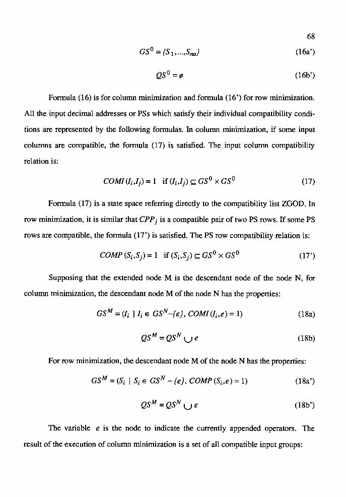
GS0 = {S 1 • .. .,SnaJ
QSo =¢
68
(16a')
(16b')
Formula (16) is for column minimization and formula (16') for row minimization.
All the input decimal addresses or PSs which satisfy their individual compatibility condi
tions are represented by the following formulas. In column minimization, if some input
columns are compatible, the formula (17) is satisfied. The input column compatibility
relation is:
COMI(Ii,/j) = 1 if (Ii,/j) c GS0 x GS0 (17)
Formula (17) is a state space referring directly to the compatibility list ZGOD. In
row minimization, it is similar that CPPj is a compatible pair of two PS rows. If some PS
rows are compatible, the formula (17') is satisfied. The PS row compatibility relation is:
COMP (Si,Sj) = 1 if (Si,Sj) c GS0 x GS0 (17')
Supposing that the extended node Mis the descendant node of the node N, for
column minimization, the descendant node M of the node N has the properties:
asM =(Ii I Ii e asN-(eJ, COMI(Ii,e) = 1)
QSM =QSN ue
(18a)
(18b)
For row minimization, the descendant node M of the node N has the properties:
asM =(Si I si e asN - (eJ, COMP(Si,e) = 1)
QSM =QSN ue
(18a')
(18b')
The variable e is the node to indicate the currently appended operators. The
result of the execution of column minimization is a set of all compatible input groups:
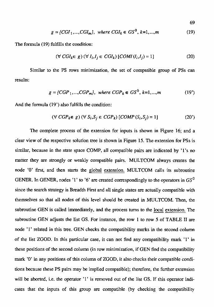
g ={CG/ 1 •... ,CGimJ, where CGh e GS0 , k=l, ... ,m
The formula (19) fulfills the condition:
('if CGhe g) ('if Ii,Jj e CGh) [COMJ(Ji,Jj) = l]
69
(19)
(20)
Similar to the PS rows minimization, the set of compatible group of PSs can
results:
g = {CGP1, ... ,CGPmJ, where CGPk e GS0, k=l, ... ,m (19')
And the formula (19') also fulfills the condition:
('if CGPke g) ('if Si,Sj e CGPk) [COMP (Si,Sj) = l] (20')
The complete process of the extension for inputs is shown in Figure 16; and a
clear view of the respective solution tree is shown in Figure 15. The extension for PSs is
similar, because in the state space COMP, all compatible pairs are indicated by '1 's no
matter they are strongly or weakly compatible pairs. MUL TCOM always creates the
node 'O' first, and then starts the global extension. MULTCOM calls its subroutine
GENER. In GENER, nodes '1' to '6' are created correspondingly to the operators in GS0
since the search strategy is Breadth First and all single states are actually compatible with
themselves so that all nodes of this level should be created in MUL TCOM. Then, the
subroutine GEN is called immediately, and the process turns to the local extension. The
subroutine GEN adjusts the list GS. For instance, the row 1 to row 5 of TABLE II are
node '1' related in this tree. GEN checks the compatibility marks in the second column
of the list ZGOD. In this particular case, it can not find any compatibility mark '1' in
these positions of the second column (in row minimization, if GEN find the compatibility
mark 'O' in any positions of this column of ZGOD, it also checks their compatible condi
tions because these PS pairs may be implied compatible); therefore, the further extension
will be aborted, i.e. the operator 'l' is removed out of the list GS. If this operator indi
cates that the inputs of this group are compatible (by checking the compatibility

70
condition), this operator will be added to a list MUS Tl. Then, the array QS collects the
contents of MUS Tl and appends the content of the operator '1 '. Otherwise, it is just
deleted from GS. After this step, GEN turns to the node '2'. So far, it is found that from
the row 6 to row 9 of the first column of ZGOD, there is only one 'l' at the 8th row and
the first column of this table indicates '2' and '5'. Therefore, the extension is executed,
That is, the operator '5' is put on the AS list and the new node '7' is created. After this,
the further local extension becomes impossible because there is no operator compatible
with both '2' and '5' simultaneously. As a result, GEN creates the new node '7' which
presents the CGI = { 2, 5} and then gives up this branch of the tree and backtracks to
node '3'.
The process creates all the compatible groups. These CGs are transferred from QS
into a two dimensional array TABIMP one after one and the numbers of the elements of
these groups are contained in another array FC. Meantime, it lists all the nodes created by
subroutine GEN as the new operators in array GS. All this information will be given out
when the subroutine GEN completes its work.
§ 4.3. CALLING TO MULTCOM FOR CREA TING MCCS
The second calling to MULTCOM is to create all the minimal closed and com
plete coverings. The operators in this calling are the addresses of the CGs created by the
last calling (in column minimization they are the numbers of the CGis; and in row
minimization they are the numbers of the CGPs) indicated by the array GS.
For explaining the difference between the complete coverings of input columns
and the closed and complete coverings of PS rows, the merger graph can be used again.
Referring to the discussion about this graph from previous sections, each node of this
graph represents an input or a PS. If two nodes are compatible, one connection must exist
between them. If the connections among several nodes are complete, which means these
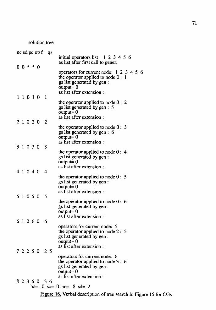
solution tree
nc sd pc op f qs
0 0 * * 0
1 1 0 1 0 1
2 1 0 2 0 2
3 1 0 3 0 3
4 1 0 4 0 4
5 1 0 5 0 5
6 1 0 6 0 6
7 2 2 5 0 2 5
8 2 3 6 0 3 6
initial operators list : 1 2 3 4 5 6 as list after first call to gener:
operators for current node: 1 2 3 4 5 6 the operator applied to node 0 : 1 gs list generated by gen : output= 0 as list after extension :
the operator applied to node 0 : 2 gs list generated by gen : 5 output= 0 as list after extension :
the operator applied to node 0 : 3 gs list generated by gen : 6 output= 0 as list after extension :
the operator applied to node 0 : 4 gs list generated by gen : output= 0 as list after extension :
the operator applied to node 0 : 5 gs list generated by gen : output= 0 as list after extension :
the operator applied to node 0 : 6 gs list generated by gen : output= 0 as list after extension :
operators for current node: 5 the operator applied to node 2 : 5 gs list generated by gen : output= 0 as list after extension :
operators for current node: 6 the operator applied to node 3 : 6 gs list generated by gen : output= 0 as list after extension :
be= 0 sc= 0 nc= 8 sd= 2
Figure 16. Verbal description of tree search in Figure 15 for CGs
71

72
nodes and connections satisfy the formula ( 10), the nodes within this complete clique
satisfy the closed and complete conditions.
Supposing that the nodes 'l' and '2' from Figure 17(a) are in such a CGI, for
column minimization, just remove this compatible group from the graph and disconnect
the connections between the nodes in this group and the nodes left in the remaining
graph. After this step is done, the connections between the nodes '1' and '4', '1' and '3'
as well as '2' and '3' are no longer retained.
All compatible groups have been created in the first calling to MUL TCOM
(includes the maximal compatible groups, i.e. the maximal complete cliques shown in
merger graph) and their compatibilities have been proven. Therefore, it is not necessary
to check again for column minimization in the second calling to MUL TCOM. However,
in row minimization, this problem is relatively more complicated. The difficulty is that in
the row minimization, using the same graph coloring method as in the column minimiza
tion, may cause some CGPs to lose their credit of compatibility. Moreover, it will result
in the creation of a wrong solution.
Supposing that a merger graph of Figure 17(a) is employed to minimize the rows
of TABLE IV, one solution { 12, 34} may be created. This solution is derived by the
same version of the merger graph as the one used in column minimization or by the
second calling to MULTCOM without checking the compatibility. On the surface, this
solution indeed satisfies the definitions (1) and (6), and also satisfies the formula (1)
because both of the groups { 1, 2} and {3, 4} are compatible. Unfortunately, this set is not
a correct solution. Reviewing definitions (3) and (5), it is found that choosing the MCCP
must consider the relation of implication between {Sil and (S'h,il· The merger graph as
the one of Figure 17(a), however, does not illustrate this relationship.
Another sort of merger graph is shown in Figure 17 (b) for solving the row minim
ization problem. Supposing that there are some implied NS group {S' mJ in a certain COP
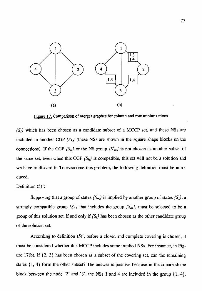
73
(a) (b)
Figure 17. Comparison of merger graphes for column and row minimizations
{Si} which has been chosen as a candidate subset of a MCCP set, and these NSs are
included in another CGP {Sh} (these NSs are shown in the square shape blocks on the
connections). If the CGP {Sh} or the NS group {S' ,,J is not chosen as another subset of
the same set, even when this CGP {Shl is compatible, this set will not be a solution and
we have to discard it. To overcome this problem, the following definition must be intro
duced.
Definition (5)':
Supposing that a group of states {S,,J is implied by another group of states {S1}, a
strongly compatible group {Sh} that includes the group {Sm}, must be selected to be a
group of this solution set, if and only if {Sz} has been chosen as the other candidate group
of the solution set.
According to definition (5)', before a closed and complete covering is chosen, it
must be considered whether this MCCP includes some implied NSs. For instance, in Fig
ure 17 (b ), if { 2, 3} has been chosen as a subset of the covering set, can the remaining
states { 1, 4} form the other subset? The answer is positive because in the square shape
block between the node '2' and '3', the NSs 1 and 4 are included in the group {1, 4}.

74
Therefore, the result is MCCP = { 23, 14}.
Usually, this problem can not be solved so easily. For instance, the implied com
patible group { 1, 2} has been chosen. In this particular case, node '1' must be left in the
remaining graph. Another subset of this CCP has to be { 1, 3, 4}. As a result, the solution
CCP = { 12, 134} is returned. This overlapping solution, however, can still be a MCCP
only in cases when the non-overlapping solution does not exist. This idea will also be
used to improve the routine MULTCOM.
Since the routine MULTCOM is called to select a minimal solution among more
than one solution, the Branch and Bound strategy is chosen, and the strategy Ordering is
added on this task for speeding up the procedure. The parameters used for this goal are
stored in the data file 'fort.4':
GENAS = 1: cause the subroutine GENER to link the subroutine GEN for
creating the descendant nodes.
EQUI = 1: add subroutine EQUI for dealing with equivalent operators
(this parameter is not used in column minimization because the compati
ble input columns are never overlapped).
MUST = 1: add subroutine MUSTO for appending the indispensable
operators to the list MUSTl.
SPRAW = 1: check the newly created node if this expansion is necessary.
ORD = 1: add subroutine ORD for ordering the operators in decreasing
quality values. The operator which has the highest Q value will be dealt
first.
SELECT = 2: select the node which has the highest value of quality func
tion.
NCMAX = 1000: limit the number of selected nodes.

75
A special parameter which is created by the algorithm itself is OUTPUT. If OUT
PUT = 0, the created node is a branch. If OUTPUT = 1, the created node is an end of the
tree. If OUTPUT = 2, the created nodes of this branch create a minimal solution.
Starting from the initial node 'O', the contents of the arrays for this procedure are
as follows:
GS0 = {CG/1, .. .,CGinJ (22a)
is a set of operators.
o r· . J AS = t 1,. . ., lmx (22b)
is a set of inputs.
QSo =¢ (22c)
and the relation of covering states by compatible groups is:
COI(i;,CGlj) = 1 if (i; e CGij, (i;,CGij) cAS 0 x GS0) (23)
For row minimization, the following formulas are available.
GS 0 = {CGP1, ... ,CGPnJ (22a')
is a set of operators.
AS0 = {si, ... ,snaJ (22b')
is a set of PSs.
QSO =¢ (22c')
and the relation of covering states by compatible groups is:
COP (s;,CGPj) = 1 if (s; e CGPj, (s;,CGPj) c ASo x GSo) (23')
and the closure relation:
CLP (CGP;,CGPj) = 1 if (CGP; ~ CGPj, (CGP;,CGPj) c GS0 x GS0) (23")
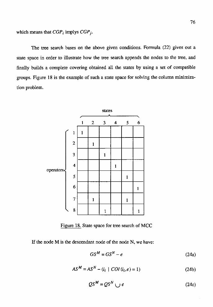
76
which means that CGPi implys CGPj.
The tree search bases on the above given conditions. Formula (22) gives out a
state space in order to illustrate how the tree search appends the nodes to the tree, and
finally builds a complete covering obtained all the states by using a set of compatible
groups. Figure 18 is the example of such a state space for solving the column minimiza
tion problem.
states
1 2 3 4 5 6
1 1
2 1
3 1
4 '
1 operators
I
5 1
6 1
7 1 1
8 1 1
Figure 18. State space for tree search of MCC
If the node Mis the descendant node of the node N, we have:
csM =GSN -e
ASM =ASN - (ii I COI(ii,e) = 1)
QSM =QSN ue
(24a)
(24b)
(24c)
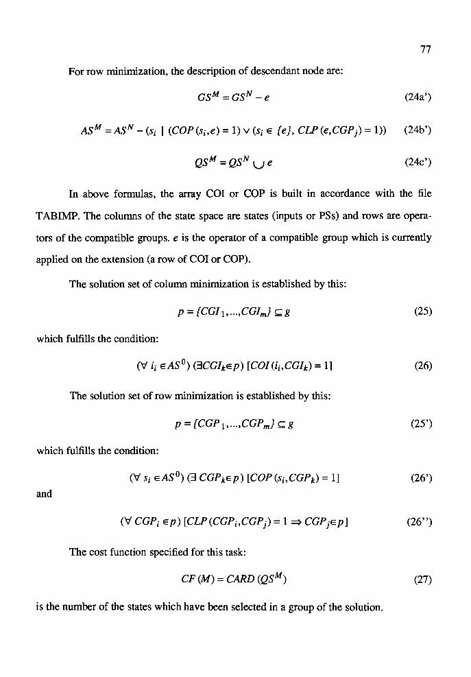
77
For row minimization, the description of descendant node are:
GSM = GSN - e (24a')
ASM =ASN - (si I (COP (si,e) = 1) v (si e {e}, CLP (e,CGPj) = 1)) (24b')
QSM = QSN U e (24c')
In above formulas, the array COI or COP is built in accordance with the file
TABIMP. The columns of the state space are states (inputs or PSs) and rows are opera
tors of the compatible groups. e is the operator of a compatible group which is currently
applied on the extension (a row of COI or COP).
The solution set of column minimization is established by this:
p ={CG! 1, ... ,CGI,,J cg (25)
which fulfills the condition:
(Vii eAS0) (3CG/kep) [COI(ii,CG/t) = l] (26)
The solution set of row minimization is established by this:
p = {CGPi. ... ,CGPmJ ~g (25')
which fulfills the condition:
(V Si eAS 0) (3 CGPkep) [COP (si,CGPk) = l] (26')
and
(V CGPi ep) [CLP(CGPi,CGPj) = 1 ~ CGPjep] (26")
The cost function specified for this task:
CF(M) =CARD (QSM) (27)
is the number of the states which have been selected in a group of the solution.
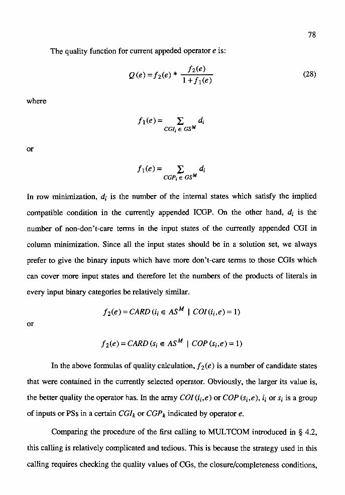
where
or
The quality function for current appeded operator e is:
/2(e) Q(e) =/2(e) * 1 + /1(e)
fi(e) = r, di cc1j e csM
/1(e) = r, di CGPi E GSM
78
(28)
In row minimization, di is the number of the internal states which satisfy the implied
compatible condition in the currently appended ICGP. On the other hand, di is the
number of non-don't-care terms in the input states of the currently appended CGI in
column minimization. Since all the input states should be in a solution set, we always
prefer to give the binary inputs which have more don't-care terms to those CGis which
can cover more input states and therefore let the numbers of the products of literals in
every input binary categories be relatively similar.
/2(e) =CARD (ii e ASM I COI(ii,e) = 1)
or
/2(e) =CARD (si e ASM I COP (si,e) = 1)
In the above formulas of quality calculation, / 2(e) is a number of candidate states
that were contained in the currently selected operator. Obviously, the larger its value is,
the better quality the operator has. In the array COI(ii,e) or COP (si,e), ii or Si is a group
of inputs or PSs in a certain CG/k or CGPk indicated by operator e.
Comparing the procedure of the first calling to MUL TCOM introduced in § 4.2,
this calling is relatively complicated and tedious. This is because the strategy used in this
calling requires checking the quality values of CGs, the closure/completeness conditions,

79
as well as the cost of the solution sets.
Q
GQ Figure 19. Solution tree for creating MCC
The complete process of this calling to MULTCOM is as follows. MUL TCOM
calls GENER. GENER is the procedure of finding indispensable operators and applying
them to extend the related node. The first cycle for global extension starts from the sub
routine GENER. At first, GENER calls EQUI for deleting the equivalent node. Secondly,
it calls MUSTO for searching the indispensable operators and applying them in list
MUSTl. Thirdly, it calls GEN for checking the closure and completeness conditions. In
the modified version of GEN in this thesis, if the procedure is for handling the row
minimization, the array SMAX which contains the compatible conditions is checked for
the closure of these CGs. This checking involves only those implied compatible groups
(ICGP) and the result of the first calling to MULTCOM is used directly. As a contrast,
this procedure is simply avoided in column minimization. In subroutine MUSTO, the list
MUSTl becomes empty if there is no more indispensable operator in the candidate list
GS; then the routine GENER terminates.
Here, MULTCOM puts the data generated by GENER in a long term list and then
orders the operators by calling to subroutine ORD. The second cycle starts from GENER
again. It performs in the same way as the first cycle discussed above, but the goal of this

80
cycle is the local extension.
The meaning of Branch and Bound is: Every time a search comes into a branch of
the tree, this search turns to a local extension from the global extension. If a node in this
local extension will be able to lead to a successive tree search, i.e., the extended nodes
tend to have better values of the quality functions and less overlappings, this extension
will continue; otherwise, this extension will be cut off and the backtrack occurs.
Generally, in both global and local extensions, if the tested operators satisfy the
condition described in the last paragraph, this extension is successive, and a new node is
created. If the compatible groups added to this node satisfy the closed and complete con
ditions, these CGs may consist of a minimal solution set. When a solution is created, all
of the indispensable operators which are involved in the extended nodes in a path of the
tree have been stored in the array QS. The completeness checking is to compare all of the
PS rows indicated by these operators with the list of PS rows in the array GS. If all of the
PS rows have been presented, this solution is complete. On the other hand, for column
minimization, this process is relatively simple because the closure checking is not neces
sary. If all of the operators can pass the above checking, finally this procedure calculates
these operators' value of cost function by calling to the subroutine FOC(f).
Figure 19 shows the example of this process for searching the minimal solution.
Its verbal expression is shown in Figure 20. The input of this process is the list of compa
tible groups stored in array TABIMP shown in TABLE III. In global search, the
indispensable operators '1' and '4' have been chosen as the subsets of any minimal solu
tion. In the second step (the description of global extension), these two operators are put
in list MULTl. Therefore, they will no longer appear in the local search. After calling to
the ordering subroutine ORD, the operators '7' and then '8' are chosen for local exten
sion, because they have higher quality values. In the following steps, the elements
represented by operators '2', '3', '5' and '6' are checked. The result is that they have
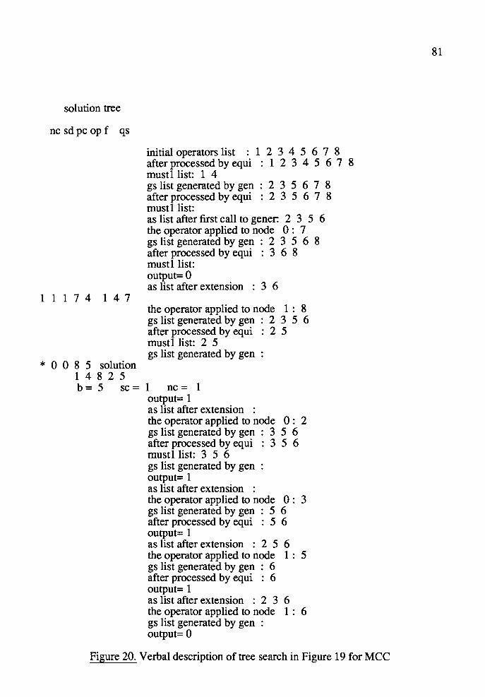
solution tree
nc sdpc op f qs
1 1 1 7 4 1 4 7
* 0 0 8 5 solution 1 4 8 2 5
initial operators list : 1 2 3 4 5 6 7 8 after processed by equi : 1 2 3 4 5 6 7 8 mustl list: 1 4 gs list generated by gen : 2 3 5 6 7 8 after processed by equi : 2 3 5 6 7 8 mustl list: as list after first call to gener: 2 3 5 6 the operator applied to node 0 : 7 gs list generated by gen : 2 3 5 6 8 after processed by equi : 3 6 8 mustl list: output= 0 as list after extension : 3 6
the operator applied to node 1 : 8 gs list generated by gen : 2 3 5 6 after processed by equi : 2 5 mustl list: 2 5 gs list generated by gen
b = 5 sc = 1 nc = 1 output= 1 as list after extension : the operator applied to node 0 : 2 gs list generated by gen : 3 5 6 after processed by equi : 3 5 6 mustl list: 3 5 6 gs list generated by gen output= 1 as list after extension : the operator applied to node 0 : 3 gs list generated by gen : 5 6 after processed by equi : 5 6 output= 1 as list after extension : 2 5 6 the operator applied to node 1 : 5 gs list generated by gen : 6 after processed by equi : 6 output= 1 as list after extension : 2 3 6 the operator applied to node 1 : 6 gs list generated by gen : output= 0
Figure 20. Verbal description of tree search in Figure 19 for MCC
81

2 1 1 6 4 1 4 6
1 4 7 8
as list after extension : 2 3 5
operators for current node: 3 6 8 the operator applied to node 1 : 8 gs list generated by gen : 3 6 * 1 0 8 4 solution
b = 4 sc = 2 nc = 2 output= 1 as list after extension : the operator applied to node 0 : 3 gs list generated by gen : 6 output= 1 as list after extension : 6 the operator applied to node 1 : 6 gs list generated by gen : output= 1 as list after extension : 3
the last solution is optimal be= 7 sc= 2 nc= 2 sd= 1 The Final Solution List:
1 4 7 8
Figure 20. Verbal description of tree search in Figure 19 for MCC (continue)
82
already been involved in the compatible groups represented by operators '7' and '8'
respectively. As a result, they are deleted from the list GS by subroutine EQUI before the
nodes t 1 , t 2, t3 and t4 are formed. Finally, the procedure creates the minimal solution
MCCI = { 1, 4, 25, 36}.
§ 4.4. CALLING TO MUL TCOM FOR INPUT COMBINATIONAL COVERING
The relative content of this process has been discussed at the end of § 2.4. The
minimization of the covering table of Figure 12(a) is actually such a problem. For refer
ence to this problem, the approach of M. Perkowski and J. Liu [15] is available.
Since this problem can be solved by using a similar method to the second calling
to MULTCOM for solving the state table minimization problem introduced in§ 4.3, the
Branch and Bound strategy is recommended. The parameters and data used in this prob
lem are the same as in the procedure for creating the MCCs in the second calling to
MUL TCOM. Some differences are in the setting of the initial conditions, in the process

83
methods for finding the equivalent groups in subroutine EQUI, and for picking up the
indispensable subsets in subroutine MUSTO. In this input logic encoding problem,
MULTCOM is called only once since the minterms have been found by the tabulation
procedure (they can be considered the same as CGs in state table minimization). This
only calling to MUL TCOM is for finding the minimal complete covering.
Comparing with the state table minimization algorithms, the features of this algo
rithm are:
(1) In MUSTO, the indispensable operators are checked by the numbers indi
cated in array FC. For instance, if a certain number is 1, this row has only
oneX.
(2) In EQUI, comparing any two rows of the covering table, if row i has the
same or less numbers of Xs and all these Xs are in the same columns with
row j or included in some columns of row j, row i is called equivalent
with row j; therefore, this row i should be deleted from list GS.
(3) The same as in the second calling to MULTCOM for column minimiza
tion, the checking of the compatibility is not necessary; therefore, the
algorithm in subroutine GEN becomes relatively simpler.
(4) Since the closure condition is not necessary to be checked (the same as in
the second calling to MULTCOM for column minimization), but the over
lap is sometimes still not avoidable.
GSo = {R l • ... ,Rm} (29a)
is the set of operators of binary prime implicants shown at the left side of the covering
table in Figure 12(a).
AS0 = {C 1 • .. .,CnJ (29b)
is the set of covering indicators shown at the heading of Figure 12(a).
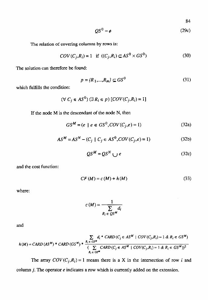
QSO =¢
The relation of covering columns by rows is:
COV(Cj,Ri) = 1 if ((Cj,Ri) ~ AS 0 x GS0)
The solution can therefore be found:
P = {R 1 ••• .,Rm.J c GSo
which fulfills the condition:
(\:/ Cj E AS0 ) (3 Ri E p) [COV(Cj.Ri) = l]
If the node Mis the descendant of the node N, then
GsM =(e I e e Gs0 ,COV(Cj,e)= 1)
ASM =ASN -(Cj I cj E AS0 ,COV(Cj,e) = 1)
QSM =QSN ue
and the cost function:
where:
and
CF(M) = c(M) + h(M)
1 c(M) = L di
M R; E QS
84
(29c)
(30)
(31)
(32a)
(32b)
(32c)
(33)
L d; * CARD (C; E ASM I cov (C;.R;) = 1 & R; E GSM) M R;e GS111
h (M) =CARD (ASM) * CARD (GS ) * ( L CARD (C; E ASM I COV(C;.R;) = 1 & R; E GSM))2
R;e GS111
The array COV(Cj,Ri) = 1 means there is a X in the intersection of row i and
column j. The operator e indicates a row which is currently added on the extension.
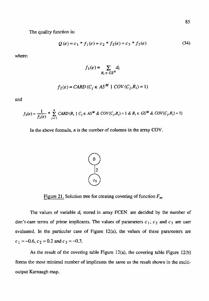
85
The quality function is:
Q(e)=c 1 * fi(e)+c2 * /2(e)+c3 * /3(e) (34)
where:
fi(e) = 1: di Rj e csN
f2(e) =CARD (Cj e ASM I COV(Cj,Ri) = 1)
and
1 11
f 3(e) = -1
( ) * L CARD (Ri I Ci e ASM & COV(Cj,Ri) = 1 & Ri e GSM & COV(Cj,Ri) = 1) 2 e i= 1
In the above formula, n is the number of columns in the array COV.
~ Q
Figure 21. Solution tree for creating covering of function Fm
The values of variable di stored in array FCEN are decided by the number of
don't-care terms of prime implicants. The values of parameters c 1, c 2 and c3 are user
evaluated. In the particular case of Figure 12(a), the values of these parameters are
c 1 = -0.6, c2 = 0.2 and c3 = -0.3.
As the result of the covering table Figure 12(a), the covering table Figure 12(b)
forms the most minimal number of implicants the same as the result shown in the multi-
output Karnaugh map.

solution tree
nc sd pc op f qs
* 0 0 2 4 solution 1 3
initial operators list : 1 2 3 after processed by equi : 1 2 3 mustl list: 1 3 gs list generated by gen : 2
b = 4 sc = 1 nc = 0 as list after first call of gener:
the last solution is optimal be= 1 sc= 1 nc= 0 sd= 0
Figure 22. Verbal description of tree search in Figure 21 for MCC
86
The search for the minimal covering can be done by MULTCOM. The operators
of the input data from the left side of Figure 12(a) and the indicators of the covering from
the heading of the same table are put in the array TABIMP shown in TABLE XII in this
tree search. The process of the tree search is shown in Figure 21 and its verbal descrip
tion is in Figure 22. This process is similar to the search for MCCs in the second calling
to MULTCOM. In the global search, MULTCOM finds that the operators '1' and '3' are
indispensable. Therefore, these compatible groups of two operators are chosen as the
parts of solution and nodes t 1 and t 2 are deleted before they are formed. In the next step,
MULTCOM finds that the operator 2 has been covered by operators '1' and '3'. There
fore, the node t 3 is also deleted and the compatible group of operator '2' will not be put
in the solution. The minimal closed and complete covering includes only the compatible
groups of operators '1' and '3'.

CHAPTER V
CONCLUSION
The complete program Two Dimensional FSM Minimizer TDFM discussed in
this thesis has been tried out on several Finite State Machines. Some of those machines
contain as many as 50 present states, some contain 20 inputs. From the results of these
trials, it appears that TDFM is able to deal with large scale machines and generates the
optimal solutions more quickly, if the percentage of don't care terms in these machines
is lower. As the percentage of don't care terms increases, the time needed in generating
the MCCPs will obviously expand. This is because that even though the generation of
compatible groups is a fast process, the identification of the compatibility, especially the
identification of feasibility for the closed and complete covering is usually a tedious pro
cess in row minimization problem. This identification includes not only the testing of
compatibility among the corresponding NSs of those CGPs but also the implied compati
bility among the ICGPs and other related compatible PS groups.
Another cause of the complication is related to the strategy setting. In the second
calling to MUL TCOM for generating the MCCP of row minimization, the parameter
SPRA W, for instance, is used to perform the branch and bound strategy. It orders the
algorithm to compare every newly generated node with all its parent nodes for deciding
each new node's quality. Since the large scale machines always produce a giant tree
structure, this comparison will unavoidably involve all the nodes in the established part
of the tree. The process will be considerably slowed down.
The last reason for this complication is that since the program deals with the
column and row minimizations iteratively, the more don't care terms exist in the initial

88
machine M 0 , the more times of the iterations will be applied to create both of OMCCI
and OMCCP of a FSM M*.
The questions discussed above do not mean that the program TDFM is not
efficient or even not practical. In fact, TDFM was the only program aimed at the large
scale machines with a relative high percentage of don't care terms. Therefore, the time
spent on the procedure is reasonably worthwhile since as it is known that there is not any
other time saving program or even the theory that can construct such a program for state
table minimization yet The AI program MUL TCOM is still based on the trial-and-error
theory. Up to now, this program has been able to compare the present node with its
parent nodes to decide its quality; but the cost of the solution and qualities of the esta
blished nodes are still not anticipatable. Presently, the methodology to save time is the
suitable selection of the strategies, as well as the suitable selection of the cost function
and quality function.
The theory about AI technology applied in MUL TCOM can be found in the refer
ence book "Problem Solving Methods in Artificial Intelligence" [16]. Additionally, a
study done by E. Lawler, 1966 [17] has discussed the method of branch and bound.
The algorithm of tabulation and then the selection of the minimal binary input
covering will not spend a lot of time, since the size of the machine has already been
reduced in previous minimization procedures. Even for those slightly reduced large scale
machines, time is still not a problem because it is a combinational logic question. In addi
tion, the testing of compatibility in MUL TCOM is simpler as has been discussed in § 4.4.
For the same reason, the column minimization hires a similar form of MUL TCOM in the
second calling for solving the closed and complete covering problem. Therefore, the
behavior of this problem can also be similar to the binary input covering problem.
Some machines have been practised on the program TDFM. The statistical results
of these machines are listed in TABLE XIX.
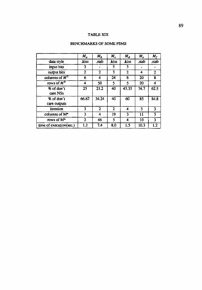
89
TABLE XIX
BENCHMARKS OF SOME FSMS
Ma Mb Mc M4 M. M1 data style .kiss .stab .kiss .kiss .stab .stab input bits 3 - 5 3 - -
output bits 2 2 3 2 4 2 columns of Mu 6 4 24 6 20 8
rows of Mu 4 50 5 5 20 4 % of don't 25 21.2 40 43.33 74.7 62.5 careNSs
% of don't 66.67 34.24 40 60 85 84.8 care outputs
iteration 3 2 2 4 3 3 columns of M* 3 4 19 3 11 3
rowsofM* 2 46 5 4 10 3 time of execution(sec.) 1.3 7.4 8.0 1.5 10.3 1.2
REFERENCES
[1] Paul M.C. and Unger, S.H. : "Minimizing the Number of States in Incompletely Specified Sequential Switching Functions", IRE Trans. Electron. Computers, Vol. EC-8, pp. 356-367, Sept. 1959.
[2] Unger, S.H.: "Flow Table Simplification - Some Useful Aids", IEEE Transaction on Electron. Computers (short notes), Vol. EC-14, pp. 472-475, June 1965.
[3] McCluskey, E.J. : "Minimum-State Sequential Circuits for a Restricted Class of Incompletely Specified Flow Tables", Bell System Tech. J., pp. 1759- 1768, Nov. 1962.
[4] Pager, D.: "Conditions for the Existence of Minimal Closed Covers Composed of Maximal Compatibles", IEEE Transaction on Computers. (short notes), Vol. C-20, pp. 450-452, April 1971.
[5] Enrich, H. : "A Note on State Minimization of a Special Class of Incomplete Sequential Machines", IEEE Transaction on Computers (short notes), Vol. C-21, pp. 500-502, May 1972.
[6] Grasselli, A. and Luccio, F.: "A Method for Minimizing the Number of Internal States in Incompletely Specified Sequential Networks", IEEE Transaction on Electron. Computers, Vol. EC-14, pp. 350-359, June 1965.
[7] Luccio, F.: "Extending the Definition of Prime Compatibility Classes of States in Incomplete Sequential Machine Reduction", IEEE Transaction on Computers, Vol. C-18, pp. 537-540, June 1969.
[8] Hamachi, G.: "Peg Tutorial", VLSI Tools, Univ. of California, Berkeley, 1984.
[9] Perkowski, M. and Nguyen, N. : "Minimization of Finite State Machines in SuperPeg", Proceeding of the Midwest Symposium on Circuits and Systems. Louisville, Kentucky, 22-24 .pp 139-147, August 1985.
[10] Biswas, N. N. : "State Minimization of Incompletely Specified Sequential Machines", IEEE Transaction on Computers, Vol. C-23, pp. 80-84, 1974.
[11] Yamamoto, M. : "A Method for Minimizing Incompletely Specified Sequential Machines" , IEEE Transactions on Computers, Vol. C-29, No. 8, pp. 732-736, August 1980.
91
[12] Perkowski, M. and Uong, H. : "Automatic Design of Finite State Machines with Electronically Programmable Devices", Record of Northcon 87, Portland, 1987, paper 13/4.
[13] De Micheli, G., Brayton, R. and Sangiovanni-Vincentelli, A.L. : "Optimal State Assignment for Finite State Machines", IEEE Transactions on Computer-Aided Design, Vol. CAD-4, No. 3, pp. 269-285, July 1985.
[14] Perkowski, M. : "An application of General Problem Solving Methods in Computer Aided Design", The Multicomp System And Its Problem Oriented Source Language, IV Intern. Symp. Methods of Heuresis (Warsaw 1977), Vol. 3, pp. 23-90.
[15] Perkowski, M., Liu, J. and Brown J. : "A System for Fast Prototyping of Logic Design Programs", Proceedings of 1987 Midwest Conference on Circuits and Systems, Syracuse, New York.
[16] Nilsson, Nils J. : "Problems Solving Methods in Artificial Intelligence", McGraw-Hill, 1971.
[17] Lawler, E. L. and Wood, D. E. : "Branch-And-Bound Methods, A Survey", Operations Res. 14, pp. 699-719, 1966.
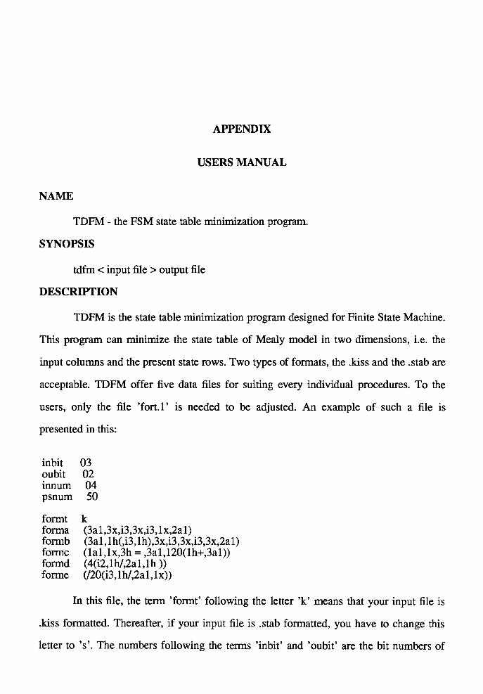
APPENDIX
USERS MANUAL
NAME
TDFM - the FSM state table minimization program.
SYNOPSIS
tdfm < input file > output file
DESCRIPTION
TDFM is the state table minimization program designed for Finite State Machine.
This program can minimize the state table of Mealy model in two dimensions, i.e. the
input columns and the present state rows. Two types of formats, the .kiss and the .stab are
acceptable. TDFM offer five data files for suiting every individual procedures. To the
users, only the file 'fort.1' is needed to be adjusted. An example of such a file is
presented in this:
in bit oubit inn um psnum
formt forma formb formc formd forme
03 02 04 50
k (3al ,3x,i3,3x,i3, lx,2al) (3al, lh(,i3, lh),3x,i3,3x,i3,3x,2al) (lal,lx,3h = ,3al,120(1h+,3al)) (4(i2,lh/,2al,lh )) (/20(i3, lh/,2al, lx))
In this file, the term 'formt' following the letter 'k' means that your input file is
.kiss formatted. Thereafter, if your input file is .stab formatted, you have to change this
letter to 's'. The numbers following the terms 'inbit' and 'oubit' are the bit numbers of
93
binary inputs and outputs. These numbers respect to the numbers of the characters that
follow the formats 'forma' to 'forme' in parentheses. For instance, all of the expressions
'3al' corresponding to the number of input bits, and all of the expressions '2al'
corresponding to the number of output bits. Moreover, the expressions 'i3' are the bits of
internal states. All of these expressions should be adjusted in the .kiss formatted input file
deponding to the bit numbers of your file. On the other hand, for suiting the .stab format
ted input file, aside above adjustments, the numbers following the terms 'innum' and
'psnum' are the numbers of the input columns and the present state rows. These two
numbers should be adjusted particularly according to the size of your .stab formatted
input file. The same as the adjustments for above formats, the number '4' following the
format 'formd' is the number of input columns whatsoever.
AUTHOR
William. Y. Zhao
FILES
/yuezhao/507 ee/store fort.1
/yuezhao/507 ee/store fort.2
/yuezhao/507 ee/store fort.3
/yuezhao/507 ee/store fort.4
/yuezhao/507 ee/store fort.5
/yuezhao/507 ee/pro tdfm
SEE ALSO
William. Y. Zhao, A New Approach of Finite State Machine Minimization