A new bounded log-linear regression model

MetrikaDOI 10.1007/s00184-013-0460-x

A new bounded log-linear regression model

HaiYing Wang · Nancy Flournoy · Eloi Kpamegan

Received: 23 April 2012© Springer-Verlag Berlin Heidelberg 2013

Abstract In this paper we introduce a new regression model in which the responsevariable is bounded by two unknown parameters. A special case is a bounded alter-native to the four parameter logistic model. The four parameter model which hasunbounded responses is widely used, for instance, in bioassays, nutrition, genetics,calibration and agriculture. In reality, the responses are often bounded although thebounds may be unknown, and in that situation, our model reflects the data-generatingmechanism better. Complications arise for the new model, however, because the like-lihood function is unbounded, and the global maximizers are not consistent estimatorsof unknown parameters. Although the two sample extremes, the smallest and thelargest observations, are consistent estimators for the two unknown boundaries, theyhave a slow convergence rate and are asymptotically biased. Improved estimators aredeveloped by correcting for the asymptotic biases of the two sample extremes in theone sample case; but even these consistent estimators do not obtain the optimal con-vergence rate. To obtain efficient estimation, we suggest using the local maximizersof the likelihood function, i.e., the solution to the likelihood equations. We prove that,with probability approaching one as the sample size goes to infinity, there exists asolution to the likelihood equation that is consistent at the rate of the square root ofthe sample size and it is asymptotically normally distributed.

H.WangDepartment of Mathematics and Statistics, University of New Hampshire, N315C Kingsbury Hall, 33Academic Way, Durham, NH 03824, USAe-mail: [email protected]

N. Flournoy (B)Department of Statistics, University of Missouri, 146 Middlebush Hall, Columbia, MO 65211, USAe-mail: [email protected]

E. KpameganClinical and Nonclinical Biostatistics, Novavax, 9920 Belward Campus Dr, Rockville, MD 20850, USAe-mail: [email protected]

123

H. Wang et al.

Keywords Asymptotics · Consistency · Linear model · Logistic model · Maximumlikelihood estimation · Parameter dependent support

1 Introduction

Consider the following regression model

log

(B − Y

Y − A

)= xTβ + ε, (1)

where Y is the response variable and A and B are the two unknown boundaries of theresponses; x denotes a p dimensional covariate vector; β is an unknown p dimensionalregression coefficient vector; ε is the error term having a normal distribution with mean0 and variance σ 2. This model does not belong to the class of generalized linear modelsbecause the transformation of Y contains unknown parameters. It also does not belongto the class of non-regular regression model studied by Smith (1994) who focused onlinear regression models with error terms having parameter dependent support. Wecall this model the bounded log-linear regression model.

Let θ = (βT, σ, A, B)T and θ0 be the true value of θ . The likelihood function of θ

based on an independent random sample {(xi , Yi ), i = 1, . . ., n} from model (1) is

Ln(θ) = (B − A)n I (A < Y(1) < Y(n) < B)

(2π)n2 σ n

∏ni=1(B − Yi )(Yi − A)

× exp

⎡⎢⎣−

∑ni=1

{log

(B−YiYi −A

)− xT

i β}2

2σ 2

⎤⎥⎦, (2)

where I (·) is the indicator function. This likelihood function is unbounded and may

become infinite along some paths; for example, let σ 2 = ∑ni=1

{log

(B−YiYi −A

)}2and

β = 0, a p-dimensional vector of zeros; then σ n ∏ni=1(B − Yi )(Yi − A) goes to 0 if

A approaches Y(1) from the left or B approaches Y(n) from the right. So the likelihoodfunction in (2) goes to infinity as θ goes to

(0T,+∞, Y(1), Y(n)

)T along some paths.Thus the global maximizer of the likelihood function is not a consistent estimator. Ifβ and σ are known, the likelihood function is bounded because it is continuous andgoes to 0 as A approaches Y(1) or −∞, or as B approaches Y(n) or ∞.

We are motivated by a special case of model (1) in which β = (a, b)T:

log

(B − Y

Y − A

)= a + bx + ε. (3)

Model (3) can be presented as

Y = B − B − A

1 + e−(a+bx+ε),

123


by which one can see its connection to the four parameter logistic model,

Y = B − B − A

1 + e−(a+bx)+ ε. (4)

The four parameter logistic model for continuous responses is also called the Emaxmodel, and it is widely used for curve-fitting, for instance, in bioassays, nutrition,genetics, calibration and agriculture. See, for example, DeLean et al. (1978), Vølund(1978), Holford and Sheiner (1981), Ratkowsky and Reedy (1986), Finke et al. (1987),Finke et al. (1989), Ernst et al. (1997), Triantafilis et al. (2000), Nix and Wild (2001),Menon and Bhandarkar (2004), MacDougall (2006), Dragalin et al. (2007), Vedenovand Pesti (2008), Sebaugh (2011), Feng et al. (2011) and the references therein. TheE(Y |x) of model (4) is often used in phase I clinical trials to model the mean responsefor Bernoulli random variables. The applications considered here, and in the afore-mentioned references, focus on continuous random variables. We take ε to have anormal distribution N (0, σ 2) for models (3) and (4).

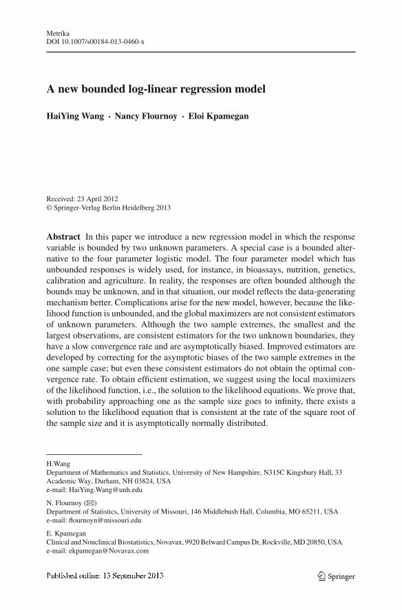
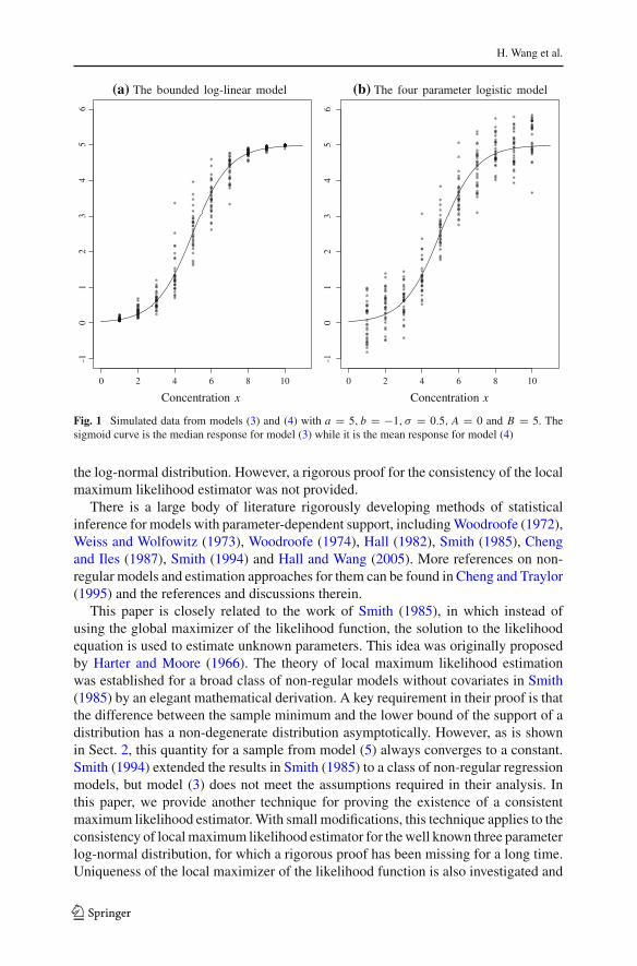
A drawback of the four parameter logistic model is that parameters A and B are ofteninterpreted as the minimum and maximum of possible responses, although model (4)allows the responses to be unbounded. Another inadequacy of model (4) is that theresponses Y have the same variance for all possible values of the covariate x , which isoften violated in practice. Leonov and Miller (2009) tackled this problem by letting thevariance of the model error depend on the covariate, but the range of possible responsesremained unbounded. Our model (3) has bounded responses and the distribution of theresponse for a given dose is skewed analogous to a beta distribution. Figure 1 displayssimulated data from models (3) and (4). Note that observations from model (4) mayfall far outside the two hypothetical bounds, while data from model (3) always staysbetween the two boundaries. Additionally, data from model (4) still has large variationin the two tails, whereas variation in the tails is skewed and very small for model (3),and this scenario is observed frequently in real data.

A special case of model (3) is, by setting b = 0 and replacing a by μ,

log

(B − Y

Y − A

)= Z , (5)

where Z ∼ N (μ, σ 2), and μ, σ, A and B are unknown parameters. Model (5) hassome similarities to the three parameter log-normal distribution, in which

log (Y − A) = Z ∼ N(μ, σ 2

),

and which also has an unbounded likelihood function (see Hill 1963). Although thethree parameter log-normal distribution has been studied by many, including Cohen(1951), Hill (1963), Harter and Moore (1966), Giesbrecht and Kempthorne (1976)and Cohen and Whitten (1980), the theoretical properties of the proposed methodswere not addressed rigorously in these papers. Cheng and Amin (1983) proposedan estimation method called maximum product spacings and proved the asymptoticnormality of the proposed estimator and the local maximum likelihood estimator for

123

H. Wang et al.

0 2 4 6 8 10

-10

12

34

56

(a) The bounded log-linear model

******************************

***

*********

*

*************

*

*** *

*

**

*****

*

*

**

**

****

*

*

*

*

*

****

*

**

*

*

**

*

*

**

***

*

*

***

***

*

*

*

*

*****

*

**

*

**

*

*

*

**

*

*

**

*

*

*

*

*

*

*

*

*****

***

*

*

**

*

***

*

*

**

*

*

*

*

*

*

*

****

*

**

*

***

**

***

*

*

*

**

**

**

*

**

*

***

***

**

**

****

****************************

******************************

******************************

Concentration x

0 2 4 6 8 10

-10

12

34

56

(b) The four parameter logistic model

**

***

**

*

*

*

*

*

*

*

****

*

*

*

*

*

**

*

*

**

*

*

**

*

*

*

*

**

**

*

*

*

*

*

**

*

***

**

*

*

*

*

*

*

*

*

*

*

**

*

**

*

*

**

**

****

*

*

*

*

*

****

*

**

*

*

*

*

*

*

**

***

*

*

**

*

***

*

*

*

*

*****

*

**

*

**

*

**

**

*

*

**

*

*

*

*

*

*

*

*

*****

***

*

*

**

*

***

*

*

**

*

*

*

*

*

*

*

****

*

**

*

***

**

**

*

*

*

*

*

*

**

**

*

*

*

*

***

***

**

**

** *

*

***

*

***

*

*

*

**

*

**

**

*

**

*

*

*

*

**

** *

*

*

*

*

*

*

*

*

**

**

**

***

*

*

*

***

*

**

*

**

*

*

**

*

**

****

**

*

**

*

**

**

**

*

*

*

*

**

*

Concentration x

Fig. 1 Simulated data from models (3) and (4) with a = 5, b = −1, σ = 0.5, A = 0 and B = 5. Thesigmoid curve is the median response for model (3) while it is the mean response for model (4)

the log-normal distribution. However, a rigorous proof for the consistency of the localmaximum likelihood estimator was not provided.

There is a large body of literature rigorously developing methods of statisticalinference for models with parameter-dependent support, including Woodroofe (1972),Weiss and Wolfowitz (1973), Woodroofe (1974), Hall (1982), Smith (1985), Chengand Iles (1987), Smith (1994) and Hall and Wang (2005). More references on non-regular models and estimation approaches for them can be found in Cheng and Traylor(1995) and the references and discussions therein.

This paper is closely related to the work of Smith (1985), in which instead ofusing the global maximizer of the likelihood function, the solution to the likelihoodequation is used to estimate unknown parameters. This idea was originally proposedby Harter and Moore (1966). The theory of local maximum likelihood estimationwas established for a broad class of non-regular models without covariates in Smith(1985) by an elegant mathematical derivation. A key requirement in their proof is thatthe difference between the sample minimum and the lower bound of the support of adistribution has a non-degenerate distribution asymptotically. However, as is shownin Sect. 2, this quantity for a sample from model (5) always converges to a constant.Smith (1994) extended the results in Smith (1985) to a class of non-regular regressionmodels, but model (3) does not meet the assumptions required in their analysis. Inthis paper, we provide another technique for proving the existence of a consistentmaximum likelihood estimator. With small modifications, this technique applies to theconsistency of local maximum likelihood estimator for the well known three parameterlog-normal distribution, for which a rigorous proof has been missing for a long time.Uniqueness of the local maximizer of the likelihood function is also investigated and

123


a theorem similar to Theorem 2 in Smith (1985) is formulated for a general regressionmodel.

The rest of this paper is organized as follows. In Sect. 2, the one sample case isaddressed and properties of estimators based on the sample extremes are derived. InSect. 3, we present the results for the local maximum likelihood estimator for theregression problem. Results of simulation experiments that are designed to investigatethe finite sample properties are contained in Sect. 4. Technical details are given in theAppendix.

2 Estimation based on the extreme order statistics for the one sample case

2.1 Naive estimators

Suppose an independent sample {Y1, . . ., Yn} is taken from model (5). If parametersA and B are estimated in advance, μ and σ can be estimated simply by ordinary least-squares. An naive approach is then to use the two sample extremes, Y(1) and Y(n), toestimate A and B, respectively, and then remove them from the sample and use therest of the sample to estimate μ and σ . We call such estimators naive. Why do thetwo sample extremes not perform well? It is not difficult to show that the two sampleextremes are consistent, but their convergence rate is very slow. The proposition belowgives asymptotic properties for these two statistics.

Proposition 1 Let

rn = {2 log n}1/2 − log log n + log(4π)

{8 log n}1/2 , sn = 1

{2 log n}1/2 .

The following convergence results hold in distribution as n → ∞:

eμ0+σ0rn

σ0sn

(1

eμ0+σ0rn− Y(1) − A0

B0 − A0

)→ G1,

e−μ0+σ0rn

σ0sn

(1

e−μ0+σ0rn− B0 − Y(n)

B0 − A0

)→ G2,

(6)

where μ0, σ0, A0 and B0 are the true values of the parameters, and G1 and G2 are twoindependent random variables having the same distribution function F(t) = e−e−t

.

Proof In the section “Proof of Proposition 1” of the Appendix.

From this convergence result, it follows that, as n → ∞,

eμ0+σ0rn(Y(1) − A0

) → B0 − A0,

e−μ0+σ0rn(B0 − Y(n)

) → B0 − A0,(7)

in distribution, which gives the rate of convergence as e−σ0rn . Since, for any α > 0,e−σ0rn nα → ∞, the rate of convergence is slower than n−α for any α > 0. But it is still

123

H. Wang et al.

faster than 1/ log n because e−σ0rn log n → 0. This proposition also tells us that theredoes not exist a constant sequence r∗

n → ∞ such that r∗n (Y(1) − A0) or r∗

n (B0 − Y(n))

converges to a non-degenerate distribution.

2.2 Bias adjusted estimators

Estimation based on the two sample extreme values can be improved by adjusting fortheir asymptotic biases. From (6) and (7), better estimators of A and B are obtained:

Aad j = Y(1) − (1 − γ σ ∗sn) (Y(n) − Y(1))

exp (μ∗ + σ ∗rn),

Bad j = Y(n) + (1 − γ σ ∗sn) (Y(n) − Y(1))

exp (−μ∗ + σ ∗rn),

(8)

where μ∗ and σ ∗ are two consistent estimates of μ and σ , respectively, and γ ≈ 0.577is the Euler–Mascheroni constant. Their asymptotic sampling properties are given bythe following convergence results:

eμ0+σ0rn

σ0(B0 − A0)sn( Aad j − A0) → γ − G1,

eμ0+σ0rn

σ0(B0 − A0)sn(Bad j − B0) → γ − G2,

in distribution. By adjusting for the asymptotic biases of the two sample extremes, theestimators in (8) improve the rate of convergence from e−σ0rn to sne−σ0rn . Althoughthis rate is also between 1/ log n and n−α for any α > 0, simulation results show thatthese estimators are much more efficient than the two sample extremes.

3 Maximum likelihood estimators

The estimators given in Sect. 2 do not possess the optimal convergence rate and theirproperties are difficult to derive when the model involves covariates. Thus we evaluatethe method of maximum likelihood estimation in this section focusing on model (1).

Denote the log-likelihood function by �n(θ). The likelihood equations are

∂�n(θ)

∂β=

n∑i=1

{log

(B−YiYi −A

)− xT

i β}

σ 2 xi = 0,

∂�n(θ)

∂σ= − n

σ+

n∑i=1

{log

(B−YiYi −A

)− xT

i β}2

σ 3 = 0, (9)

∂�n(θ)

∂ A= 1

B − A

n∑i=1

B − Yi

Yi − A−

n∑i=1

log(

B−YiYi −A

)− xT

i β

σ 2(Yi − A)= 0,

123


∂�n(θ)

∂ B= − 1

B − A

n∑i=1

Yi − A

B − Yi−

n∑i=1

log(

B−YiYi −A

)− xT

i β

σ 2(B − Yi )= 0.

In this section, following the idea of Smith (1985), we study the properties of localmaximizer of the likelihood function, i.e., the solution to the likelihood equations. Weprove the existence and consistency of the resultant estimator.

From calculations in the section “Derivation of the Fisher information” of theAppendix, the Fisher information matrix based on the sample is

In(θ)

=n∑

i=1

⎧⎪⎪⎪⎪⎪⎪⎪⎪⎪⎪⎪⎨⎪⎪⎪⎪⎪⎪⎪⎪⎪⎪⎪⎩

xi xTi

σ 2 0 −1−ci dσ 2(B−A)

xTi

−1− dci

σ 2(B−A)xT

i

0 2σ 2

−2ci dσ(B−A)

2 dci

σ(B−A)

−1−ci dσ 2(B−A)

xi−2ci d

σ(B−A)

c2i d4

(B−A)2 + 1+2ci d+c2i d4

σ 2(B−A)2−1

(B−A)2 + 2+ci d+ dci

σ 2(B−A)2

−1− dci

σ 2(B−A)xi

2 dci

σ(B−A)−1

(B−A)2 + 2+ci d+ dci

σ 2(B−A)2

d4

c2i

(B−A)2 +1+2 d

ci+ d4

c2i

σ 2(B−A)2

⎫⎪⎪⎪⎪⎪⎪⎪⎪⎪⎪⎪⎬⎪⎪⎪⎪⎪⎪⎪⎪⎪⎪⎪⎭

,

where ci = exTi β and d = eσ 2/2.

The following assumptions are required for the asymptotic results in this section.

Assumption 1 supi ‖xi‖ < ∞, where ‖ · ‖ denotes the Euclidean norm.

Assumption 2 The following quantities converge as n → ∞:n−1 ∑n

i=1 xi , n−1 ∑ni=1 xi xT

i , n−1 ∑ni=1 exT

i β , n−1 ∑ni=1 e−xT

i β , n−1 ∑ni=1 xi exT

i β ,

n−1 ∑ni=1 xi e−xT

i β , n−1 ∑ni=1 e2xT

i β and n−1 ∑ni=1 e−2xT

i β .

Assumption 3 (xT1, . . ., xT

n)T is full rank.

If the Assumptions 1-3 hold, then In(θ)/n converges to a positive-definite matrix,say I(θ).

The following theorems present the properties of the local maximum likelihoodestimator, the solution to (9). Proofs of these theorems are given in the section “Proofof Theorems for the regression model” of Appendix.

Theorem 1 (Existence) If Assumptions 1–3 hold, then with probability approaching1, there exists a sequence of solutions θn to the likelihood equations in (9) that is alocal maximizer of the likelihood function and is n1/2-consistent for θ .

Theorem 2 (Uniqueness) Assume Assumptions 1–3 hold. Let δ be some fixed valueand δn = n−α for some α > 0. Denote by Sδ = {θ : A ≤ A0−δ and B ≥ B0+δ} andTδ,n = {θ : A0−δ ≤ A ≤ A0+δn, B0−δn ≤ B ≤ B0+δ and ‖β−β0‖+|σ −σ0|>δ}.Then, for any compact set K ⊂ R

p+3,

limn→∞ Pr

{sup

Sδ∩K�n(θ) < �n(θ0)

}= 1, lim

n→∞ Pr

{sup

Tδ,n∩K�n(θ) < �n(θ0)

}= 1.

123

H. Wang et al.

Theorem 3 (Asymptotic normality) If Assumptions 1–3 hold, the n1/2-consistent esti-mator θn in Theorem 1 satisfies

n1/2(θn − θ0) → N{

0, I−1(θ0)}

in distribution.

4 Numerical examples

4.1 Simulation

In this subsection, simulation results are reported that examine the finite sample per-formance of the biased adjusted and local maximum likelihood estimators given inSects. 2 and 3. The computation was carried out using R (R Core Team 2013) andan R package called BB (Varadhan and Gilbert 2009) was used to find the solutionsto the likelihood equations. The BB package was designed to solve large systems ofnon-linear equations and to optimize high-dimensional non-linear objective functions.Although multiple solutions to the likelihood equations may exist, according to ourTheorem 2, the solution that yields the largest value of the likelihood function shouldbe chosen as the estimate. From Eq. (9), all other parameters can be written as functionsof the two boundary parameters A and B explicitly. So there are only two non-linearequations to solve to obtain estimates of A and B, and these estimates can be insertedinto the first two equations in (9) to solve for β (or μ for the one sample model) andσ. All the simulations results are based on 1,000 iterations.

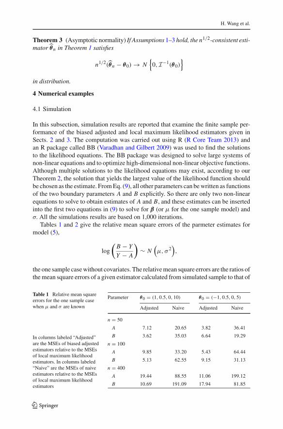
Tables 1 and 2 give the relative mean square errors of the parmeter estimates formodel (5),

log

(B − Y

Y − A

)∼ N

(μ, σ 2

),

the one sample case without covariates. The relative mean square errors are the ratios ofthe mean square errors of a given estimator calculated from simulated sample to that of

Table 1 Relative mean squareerrors for the one sample casewhen μ and σ are known

In columns labeled “Adjusted”are the MSEs of biased adjustedestimators relative to the MSEsof local maximum likelihoodestimators. In columns labeled“Naive” are the MSEs of naiveestimators relative to the MSEsof local maximum likelihoodestimators

Parameter θ0 = (1, 0.5, 0, 10) θ0 = (−1, 0.5, 0, 5)

Adjusted Naive Adjusted Naive

n = 50

A 7.12 20.65 3.82 36.41

B 3.62 35.03 6.64 19.29

n = 100

A 9.85 33.20 5.43 64.44

B 5.13 62.55 9.15 31.13

n = 400

A 19.44 88.55 11.06 199.12

B 10.69 191.09 17.94 81.85

123


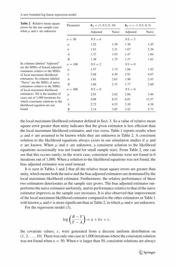
Table 2 Relative mean squareerrors for the one sample casewhen μ and σ are unknown

In columns labeled “Adjusted”are the MSEs of biased adjustedestimators relative to the MSEsof local maximum likelihoodestimators. In columns labeled“Naive” are the MSEs of naiveestimators relative to the MSEsof local maximum likelihoodestimators. NS is the number ofcases out of 1,000 iterations forwhich consistent solutions to thelikelihood equation are notfound

Parameter θ0 = (1, 0.5, 0, 10) θ0 = (−1, 0.5, 0, 5)

Adjusted Naive Adjusted Naive

n = 50 N S = 6 N S = 3

μ 1.22 1.38 1.30 1.45

σ 1.63 2.21 1.67 2.26

A 1.37 1.93 1.47 1.84

B 1.38 1.75 1.27 1.81

n = 100 N S = 2 N S = 0

μ 1.47 1.73 1.66 1.92

σ 2.68 4.30 2.91 4.67

A 1.81 2.63 1.90 2.43

B 1.66 2.15 1.77 2.60

n = 400 N S = 0 N S = 0

μ 2.01 2.62 2.66 3.46

σ 4.08 8.53 6.01 12.57

A 2.72 4.53 3.10 4.38

B 2.14 3.05 3.42 5.73

the local maximum likelihood estimator defined in Sect. 3. So a value of relative meansquare error greater than unity indicates that the given estimator is less efficient thanthe local maximum likelihood estimator, and vise-versa. Table 1 reports results whenμ and σ are assumed to be known while they are unknown in Table 2. A consistentsolution to the likelihood equations always exists in our simulation studies if μ andσ are known. When μ and σ are unknown, a consistent solution to the likelihoodequations occasionally was not found for small sample sizes. From Table 2, one cansee that this occurs rarely; in the worst case, consistent solutions were not found in 6iterations out of 1,000. When a solution to the likelihood equations was not found, thebias adjusted estimator was used instead.

It is seen in Tables 1 and 2 that all the relative mean square errors are greater thanunity, which means both the naive and the bias adjusted estimators are dominated by thelocal maximum likelihood estimator. Furthermore, the relative performance of thesetwo estimators deteriorates as the sample size grows. The bias adjusted estimator out-performs the naive estimator uniformly, and its performance relative to that of the naiveestimator improves as the sample size increases. It is also observed that improvementof the local maximum likelihood estimator compared to the other estimators in Table 1with known μ and σ is more significant than in Table 2, in which μ and σ are unknown.

For the regression model (3),

log

(B − Y

Y − A

)= a + bx + ε,

the covariate values, x , were generated from a discrete uniform distribution on(1, 2, . . ., 10). There was only one case in 1,000 iterations where the consistent solutionwas not found when n = 50. When n is larger than 50, consistent solutions are always

123

H. Wang et al.

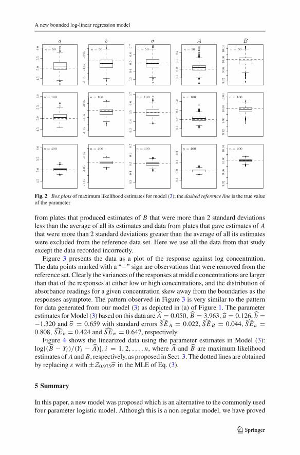
found in our studies. Table 3 gives the biases, standard errors, estimates of standarderrors and the coverage probabilities of confidence intervals with a nominal level of95 %. The biases and the standard errors are calculated from the estimates based onthe 1,000 simulated samples, while the estimates of standard errors, SE , are calcu-lated from the Hessian matrix of the likelihood function. The confidence intervals areconstructed by θ ±Z0.975 SE , where θ is the local maximum likelihood estimator andZ0.975 is the 97.5 % normal quantile. Figure 2 presents the box plots of the estimatesobtained from the 1,000 simulated samples.

It is seen that both the biases and standard errors are small, and they decrease asthe sample size increases, reflecting the consistency of the local likelihood estimator.Although it is evident that the standard errors are underestimated for small samplesizes and the coverage probabilities are lower than the nominal level, this situationameliorates as the sample size increases.

4.2 An application

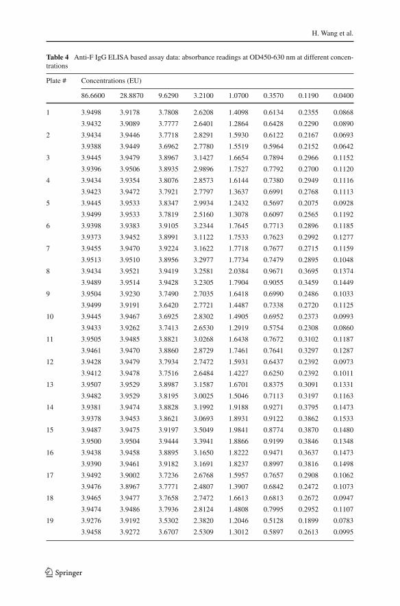
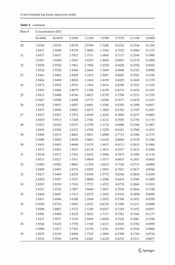
The data presented in Table 4 was generated by Kpamegan and Jani (2013) during thequalification of an Anti-F IgG ELISA based assay (FDA 2010). The study was aboutthe F protein nanoparticle vaccine. A total of 736 absorbances measured at OD450-630nanometers (nm) were taken at 8 different concentrations in ELISA units (EU) from46 plates. There were two replicates at each concentration for each plate, so we usedthe average as the responses in our analysis. There are three plates for which data wererecorded incorrectly, so we removed observations from these plates and only usedthe remaining 688 observations. In the qualification study, the four parameter logisticmodel (4) was used to fit data from each plate to determine the reference standard. Data

Table 3 Biases (×103),standard errors (×103), estimatesof standard errors (×103) andcoverage probabilities (×102)for the regression model

SE standard errors, SE estimatesof standard errors; CP coverageprobabilities

θ0 = (5, −1, 0.5, 0, 10)

a b σ A B

n = 50

Bias 234 40 53 42 15

SE 270 46 65 53 19

SEE 248 42 61 42 16

CP 90.3 90.2 92.5 84.2 84.3

n = 100

Bias 142 24 35 25 9

SE 170 29 44 31 11

SEE 170 29 43 29 11

CP 93.8 93.6 93.3 89.2 89.6

n = 400

Bias 67 11 17 12 4

SE 83 14 22 14 5

SEE 82 14 21 14 5

CP 94.5 95 94.5 93.3 94.4

123


Fig. 2 Box plots of maximum likelihood estimates for model (3); the dashed reference line is the true valueof the parameter

from plates that produced estimates of B that were more than 2 standard deviationsless than the average of all its estimates and data from plates that gave estimates of Athat were more than 2 standard deviations greater than the average of all its estimateswere excluded from the reference data set. Here we use all the data from that studyexcept the data recorded incorrectly.

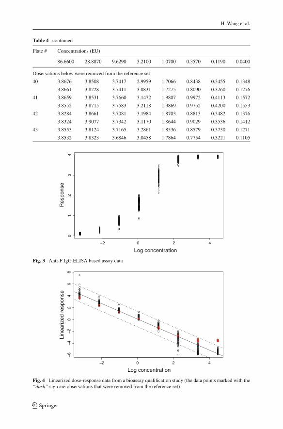
Figure 3 presents the data as a plot of the response against log concentration.The data points marked with a “−” sign are observations that were removed from thereference set. Clearly the variances of the responses at middle concentrations are largerthan that of the responses at either low or high concentrations, and the distribution ofabsorbance readings for a given concentration skew away from the boundaries as theresponses asymptote. The pattern observed in Figure 3 is very similar to the patternfor data generated from our model (3) as depicted in (a) of Figure 1. The parameterestimates for Model (3) based on this data are A = 0.050, B = 3.963, a = 0.126, b =−1.320 and σ = 0.659 with standard errors SE A = 0.022, SE B = 0.044, SEa =0.808, SEb = 0.424 and SEσ = 0.647, respectively.

Figure 4 shows the linearized data using the parameter estimates in Model (3):log{(B − Yi )/(Yi − A)}, i = 1, 2, . . . , n, where A and B are maximum likelihoodestimates of A and B, respectively, as proposed in Sect. 3. The dotted lines are obtainedby replacing ε with ±Z0.975σ in the MLE of Eq. (3).

5 Summary

In this paper, a new model was proposed which is an alternative to the commonly usedfour parameter logistic model. Although this is a non-regular model, we have proved

123

H. Wang et al.

Table 4 Anti-F IgG ELISA based assay data: absorbance readings at OD450-630 nm at different concen-trations

Plate # Concentrations (EU)

86.6600 28.8870 9.6290 3.2100 1.0700 0.3570 0.1190 0.0400

1 3.9498 3.9178 3.7808 2.6208 1.4098 0.6134 0.2355 0.0868

3.9432 3.9089 3.7777 2.6401 1.2864 0.6428 0.2290 0.0890

2 3.9434 3.9446 3.7718 2.8291 1.5930 0.6122 0.2167 0.0693

3.9388 3.9449 3.6962 2.7780 1.5519 0.5964 0.2152 0.0642

3 3.9445 3.9479 3.8967 3.1427 1.6654 0.7894 0.2966 0.1152

3.9396 3.9506 3.8935 2.9896 1.7527 0.7792 0.2700 0.1120

4 3.9434 3.9354 3.8076 2.8573 1.6144 0.7380 0.2949 0.1116

3.9423 3.9472 3.7921 2.7797 1.3637 0.6991 0.2768 0.1113

5 3.9445 3.9533 3.8347 2.9934 1.2432 0.5697 0.2075 0.0928

3.9499 3.9533 3.7819 2.5160 1.3078 0.6097 0.2565 0.1192

6 3.9398 3.9383 3.9105 3.2344 1.7645 0.7713 0.2896 0.1185

3.9373 3.9452 3.8991 3.1122 1.7533 0.7623 0.2992 0.1277

7 3.9455 3.9470 3.9224 3.1622 1.7718 0.7677 0.2715 0.1159

3.9513 3.9510 3.8956 3.2977 1.7734 0.7479 0.2895 0.1048

8 3.9434 3.9521 3.9419 3.2581 2.0384 0.9671 0.3695 0.1374

3.9489 3.9514 3.9428 3.2305 1.7904 0.9055 0.3459 0.1449

9 3.9504 3.9230 3.7490 2.7035 1.6418 0.6990 0.2486 0.1033

3.9499 3.9191 3.6420 2.7721 1.4487 0.7338 0.2720 0.1125

10 3.9445 3.9467 3.6925 2.8302 1.4905 0.6952 0.2373 0.0993

3.9433 3.9262 3.7413 2.6530 1.2919 0.5754 0.2308 0.0860

11 3.9505 3.9485 3.8821 3.0268 1.6438 0.7672 0.3102 0.1187

3.9461 3.9470 3.8860 2.8729 1.7461 0.7641 0.3297 0.1287

12 3.9428 3.9479 3.7934 2.7472 1.5931 0.6437 0.2392 0.0973

3.9412 3.9478 3.7516 2.6484 1.4227 0.6250 0.2392 0.1011

13 3.9507 3.9529 3.8987 3.1587 1.6701 0.8375 0.3091 0.1331

3.9482 3.9529 3.8195 3.0025 1.5046 0.7113 0.3197 0.1163

14 3.9381 3.9474 3.8828 3.1992 1.9188 0.9271 0.3795 0.1473

3.9378 3.9453 3.8621 3.0693 1.8931 0.9122 0.3862 0.1533

15 3.9487 3.9475 3.9197 3.5049 1.9841 0.8774 0.3870 0.1480

3.9500 3.9504 3.9444 3.3941 1.8866 0.9199 0.3846 0.1348

16 3.9438 3.9458 3.8895 3.1650 1.8222 0.9471 0.3637 0.1473

3.9390 3.9461 3.9182 3.1691 1.8237 0.8997 0.3816 0.1498

17 3.9492 3.9002 3.7236 2.6768 1.5957 0.7657 0.2908 0.1062

3.9476 3.8967 3.7771 2.4807 1.3907 0.6842 0.2472 0.1073

18 3.9465 3.9477 3.7658 2.7472 1.6613 0.6813 0.2672 0.0947

3.9474 3.9486 3.7936 2.8124 1.4808 0.7995 0.2952 0.1107

19 3.9276 3.9192 3.5302 2.3820 1.2046 0.5128 0.1899 0.0783

3.9458 3.9272 3.6707 2.5309 1.3012 0.5897 0.2613 0.0995

123


Table 4 continued


86.6600 28.8870 9.6290 3.2100 1.0700 0.3570 0.1190 0.0400

20 3.9520 3.9518 3.8276 2.9789 1.7208 0.8234 0.3346 0.1293

3.9457 3.9500 3.8370 2.9050 1.7264 0.7922 0.3064 0.1152

21 3.9477 3.9437 3.7822 2.7311 1.4848 0.7137 0.2549 0.1098

3.9467 3.9440 3.7843 2.8297 1.4640 0.6983 0.2570 0.1090

22 3.9529 3.9528 3.7861 2.7965 1.5530 0.6820 0.2556 0.0954

3.9528 3.9526 3.8368 2.6643 1.3649 0.6840 0.2783 0.0990

23 3.9461 3.9482 3.8405 3.1912 1.9987 0.8885 0.3562 0.1398

3.9464 3.9469 3.8826 3.1616 1.8199 0.8455 0.3449 0.1378

24 3.9475 3.9505 3.9535 3.1945 1.9474 0.8780 0.3552 0.1292

3.9491 3.9468 3.8679 3.1380 1.8158 0.8374 0.3624 0.1421

25 3.9413 3.9488 3.8746 3.0827 1.6729 0.7299 0.3223 0.1329

3.9447 3.9500 3.8498 2.9775 1.6568 0.7677 0.3476 0.1423

26 3.9345 3.9057 3.6507 2.6681 1.4546 0.6705 0.2498 0.0921

3.9475 3.8984 3.6092 2.6873 1.3826 0.6762 0.2395 0.1047

27 3.9427 3.9367 3.7872 2.6949 1.4249 0.5884 0.2237 0.0803

3.9459 3.9513 3.7349 2.7381 1.4122 0.7695 0.2756 0.1153

28 3.9433 3.9182 3.6337 2.4758 1.3178 0.6008 0.2368 0.1067

3.9455 3.9260 3.6322 2.4784 1.3250 0.6101 0.2560 0.1023

29 3.9499 3.9513 3.8665 2.9811 1.6988 0.7713 0.3286 0.1274

3.9490 3.9503 3.8928 2.9663 1.6165 0.8068 0.3339 0.1286

30 3.9443 3.9403 3.6609 2.9135 1.4633 0.6113 0.2615 0.1068

3.9472 3.9451 3.5953 2.6724 1.3873 0.5557 0.2433 0.1056

31 3.9530 3.9517 3.7453 2.9452 1.4906 0.7973 0.1998 0.1139

3.9527 3.9527 3.7931 3.0859 1.5577 0.6035 0.2407 0.0926

32 3.9482 3.9503 3.8863 3.1558 1.6623 0.7236 0.2731 0.0968

3.9489 3.9493 3.8743 3.0259 1.5583 0.7047 0.2817 0.0946

33 3.9437 3.9469 3.8255 2.9104 1.5772 0.6540 0.2618 0.1030

3.9420 3.9397 3.7621 2.8048 1.4306 0.6434 0.2569 0.1000

34 3.9267 3.9339 3.7424 2.7722 1.6535 0.6739 0.2664 0.1019

3.9321 3.9316 3.7097 2.8640 1.5051 0.7018 0.2844 0.1100

35 3.9469 3.9487 3.7412 2.6572 1.3382 0.5416 0.1890 0.0699

3.9451 3.9496 3.6200 2.5546 1.2652 0.5788 0.1951 0.0709

36 3.9458 3.8754 3.4593 2.2431 0.8734 0.3389 0.1211 0.0488

3.9490 3.8867 3.5123 2.1245 0.8547 0.3345 0.1451 0.0567

37 3.9501 3.9488 3.8125 2.9623 1.7317 0.7581 0.3166 0.1177

3.9471 3.9527 3.7610 2.9454 1.6028 0.7928 0.3081 0.1290

38 3.9346 3.9425 3.7578 2.7169 1.6213 0.6545 0.2392 0.0958

3.9499 3.9477 3.7383 2.6758 1.4361 0.6393 0.2544 0.0906

39 3.9525 3.9349 3.6950 2.7245 1.2856 0.5398 0.1769 0.0724

3.9524 3.9530 3.8259 2.6267 1.4229 0.6532 0.2311 0.0877

123

H. Wang et al.

Table 4 continued


86.6600 28.8870 9.6290 3.2100 1.0700 0.3570 0.1190 0.0400

Observations below were removed from the reference set

40 3.8676 3.8508 3.7417 2.9959 1.7066 0.8438 0.3455 0.1348

3.8661 3.8228 3.7411 3.0831 1.7275 0.8090 0.3260 0.1276

41 3.8659 3.8531 3.7660 3.1472 1.9807 0.9972 0.4113 0.1572

3.8552 3.8715 3.7583 3.2118 1.9869 0.9752 0.4200 0.1553

42 3.8284 3.8661 3.7081 3.1984 1.8703 0.8813 0.3482 0.1376

3.8324 3.9077 3.7342 3.1170 1.8644 0.9029 0.3536 0.1412

43 3.8553 3.8124 3.7165 3.2861 1.8536 0.8579 0.3730 0.1271

3.8532 3.8323 3.6846 3.0458 1.7864 0.7754 0.3221 0.1105

Log concentration

Res

pons

e0

12

34

−2 0 2 4

Fig. 3 Anti-F IgG ELISA based assay data

Log concentration

Line

ariz

ed r

espo

nse

−6

−4

−2

02

46

8

−2 0 2 4

Fig. 4 Linearized dose-response data from a bioassay qualification study (the data points marked with the“dash” sign are observations that were removed from the reference set)

123


that a local maximizer of the likelihood function is consistent, asymptotically normaland asymptotically efficient. Additionally, our result about the uniqueness of the MLEcan help to choose the local maximizer in practice.

When the responses of a model have unknown boundaries, one may intuitively wantto use the smallest and the largest observation to estimate them. Both our theoreticaland numerical results showed that these two statistics were not efficient for the modelproposed. Actually, since the extreme order statistics are always biased in general, oneshould always correct the bias to gain efficiency. This is also true for more generalmodels.

Acknowledgments We thank Dr. Valerii Fedorov for suggesting to us the importance of model (3).

Appendix: Technical details

Proof of Proposition 1

Proof First, following the idea in Sect. 2.3 of Galambos (1978), for any t ,

limn→∞ Pr

[{log(B0 − Y ) − log(Y − A0) − μ0

σ0

}(n)

< rn + snt

]= e−e−t

= limn→∞ Pr

{(B0 − Y

Y − A0

)(n)

< eμ0+σ0rn+σ0sn t

}

= limn→∞ Pr

{B0 − Y(1)

Y(1) − A0< eμ0+σ0rn + σ0sneμ0+σ0rn (1 + vσ0snt)t

},

where |v| ≤ 1. Since vσ0snt → 0 as n → ∞, it follows that

limn→∞ Pr

(B0 − Y(1)

Y(1) − A0< cn + dnt

)= e−e−t

,

where cn = eμ0+σ0rn and dn = σ0sneμ0+σ0rn .Then, for any t �= 0,

Pr

(B0 − Y(1)

Y(1) − A0< cn + dnt

)= Pr

(Y(1) − A0

B0 − A0>

1

1 + cn + dnt

)

= Pr

[Y(1) − A0

B0 − A0>

cn − 1

c2n

−{

dn

c2n

− (1 + dnt)

c2n(1 + cn + dnt)t

}t

].

It can be shown that [(1 + dnt)/{c2n(1+cn +dnt)t}]/(dn/c2

n) → 0 and (1/c2n)/(dn/c2

n)

→ 0 as n → ∞. So from Lemma 2.2.2 in Galambos (1978),

limn→∞ Pr

{B0 − Y(1)

Y(1) − A0< cn + dnt

}= lim

n→∞ Pr

{Y(1) − A0

B0 − A0>

1

cn− dn

c2n

t

}.

123

H. Wang et al.

When t = 0, the result can be verified by using the properties of the extreme orderstatistics of normal distribution directly. The second equation can be proved similarly.

�

Derivation of the Fisher information

The lemma below is useful in deriving the Fisher information.

Lemma 1 From Lemma 2 of Stein (1981), we obtain that, if E |h′(Z)| < ∞ for anormal random variable Z ∼ N (μ, σ 2) and some differentiable function h. Then

E{(Z − μ)h(Z)} = σ 2 E{h′(Z)}.

The log-likelihood function of model (1) based on one observation (x, Y ) is

�(θ , x, Y ) = − log (2π)

2− log σ + log(B − A) − log(Y − A)

− log(B − Y ) −{log(B − Y ) − log(Y − A) − xTβ

}2

2σ 2

for Y ∈ (A, B) and 0 otherwise. Let Z = log(B − Y ) − log(Y − A). By directcalculation,

∂�(θ , x, Y )

∂ A= 1

Y − A + (Y−A)2

B−Y

−{log(B − Y ) − log(Y − A) − xTβ

}σ 2(Y − A)

;

∂2�(θ , x, Y )

∂ A2 = 1 + 2 Y−AB−Y{

Y − A + (Y−A)2

B−Y

}2 −{log(B − Y ) − log(Y − A) − xTβ

}σ 2(Y − A)2

− 1

σ 2(Y − A)2 = e2Z + 2eZ

(B − A)2 − (Z − xTβ)(1 + eZ )2

σ 2(B − A)2 − (1 + eZ )2

σ 2(B − A)2 .

Then from Lemma 1,

E

{∂2�(θ, x, Y )

∂ A2

}= −E

{e2Z

(B − A)2 + 1 + 2eZ + e2Z

σ 2(B − A)2

}

= −e2xTβ+2σ 2

(B − A)2 − 1 + 2exTβ+ σ22 + e2xTβ+2σ 2

σ 2(B − A)2 .

Other elements of the Fisher information can be derived similarly.

Proof of Theorems for the regression model

The proof of Theorem 1 begins with some lemmas.

123


Lemma 2 For constant sequences vn ↓ v and wn ↑ w as n → ∞, let ξvn ∈ (vn+1, vn)

and ξwn ∈ (wn, wn+1). If a continuous function sequence fn(·) > 0, which is decreas-ing in n, satisfies n1+α fn(ξvn ) → 0 and n1+α fn(ξwn ) → 0 for α > 0 as n → ∞,then

lim supn

wn∫vn

fn(x)dx < ∞.

Proof Let Sn = ∫ wnvn

fn(x)dx . Then

Sn − Sn−1 =wn∫

vn

fn(x)dx −wn−1∫

vn−1

fn−1(x)dx

≤ (vn−1 − vn) fn−1(ξvn−1) + (wn − wn−1) fn−1(ξwn−1)

= (vn−1 − vn)n1+α fn−1(ξvn−1) + (wn − wn−1)n1+α fn−1(ξwn−1)

n1+α

= o

(1

n1+α

).

So lim supn Sn = lim supn∑n

i=1(Sn − Sn−1) is finite.

Lemma 3 For any α > 0, let δn = n−α . Then for any k1 ≥ 0 and k2 ≥ 0, there existsa constant M such that

limn→∞ Pr

{1

n

n∑i=1

| log(B − Yi )|k1

(Yi − A)k2< M

}= 1,

limn→∞ Pr

{1

n

n∑i=1

| log(Yi − A)|k1

(B − Yi )k2< M

}= 1

(10)

uniformly in A and B so long as |A − A0| < δn and |B − B0| < δn.

Proof We gives the details of proof for the first quantity in (10). The proof for theother one is similar.

|log(B − Yi )|k1

(Yi − A)k2= | log(B − B0 + B0 − Yi )|k1

(Yi − A0 + A0 − A)k2I (Yi − A0 > 2δn, B0 − Yi > 2δn) + op(1)

= | log(B − B0 + B0 − Yi )|k1

(Yi − A0 + A0 − A)k2I (Yi − A0 > 2δn, 1 − 2δn > B0−Yi > 2δn)

+ | log(B − B0 + B0 − Yi )|k1

(Yi − A0 + A0 − A)k2I (Yi − A0 > 2δn, B0 − Yi > 1) + op(1)

<I (Yi − A0 > 2δn, 1 − 2δn > B0 − Yi > 2δn)

(B0 − Yi − δn)k1(Yi − A0 − δn)k2

123

H. Wang et al.

+ (B0 − Yi + δn)k1

(Yi − A0 − δn)k2I (Yi − A0 > 2δn, B0 − Yi > 1) + op(1)

<I (B0 − 2δn > Yi > A0 + 2δn)

(B0 − Yi − δn)k1(Yi − A0 − δn)k2

+ (B0 − A0 + 1)k1

(Yi − A0 − δn)k2I (B0 − 1 > Yi > A0 + 2δn) + op(1)

= Cin1 + Cin2 + op(1).

Note that

(2π)12 E(Cin1) = 1

σ0

B0−2δn∫A0+2δn

1

(B0 − y − δn)k1(y − A0 − δn)k2

× B0 − A0

(B0 − y)(y − A0)exp

⎡⎢⎣−

{log

(B0−yy−A0

)− xT

i β0

}2

2σ 20

⎤⎥⎦ dy

≤ 1

σ0

B0−2δn∫A0+2δn

1

(B0 − y − δn)k1+1(y − A0 − δn)k2+1

× exp

⎡⎢⎣−

14

{log

(B0−yy−A0

)}2 − (xTi β0)

2

2σ 20

⎤⎥⎦ dy

=exp

{(xT

i β0)2

2σ 20

}

σ0

B0−2δn∫A0+2δn

1

(B0 − y − δn)k1+1(y − A0 − δn)k2+1

× exp

⎡⎢⎣−

{log

(B0−yy−A0

)}2

8σ 20

⎤⎥⎦ dy.

From Lemma 2, lim supn E(Cin1) is bounded by a finite constant, say C1. Similarly,it can also be shown that lim supn E(Cin2) is bounded by a finite constant, say C2. Sousing the formula Xn = E(Xn) + OP {var(Xn)1/2}, we have

1

n

n∑i=1

| log(B − Yi )|k1

(Yi − A)k2= 1

n

n∑i=1

E(Cin1) + 1

n

n∑i=1

E(Cin2) + OP

(n− 1

2

)+ oP (1).

Thus any M that is greater than C1 + C2 satisfys the requirement.

Lemma 4 If assumptions 1- 3 hold, then −n−1∂2�n(θ)/(∂θ∂θT) → I(θ0) in proba-bility uniformly over ‖θ − θ0‖ < δn.

123


Proof The first element of ∂2�n(θ)/(∂θ∂θT) is

∂2�n(θ)

∂ A2 =n∑

i=1

⎡⎣ 1 − 1

σ 2

(Yi − A)2 − 1

(B − A)2 −{

log(

B−YiYi −A

)− xT

i β}

σ 2(Yi − A)2

⎤⎦.

So it is straightforward to get

1

n

∣∣∣∣∂2�n(θ)

∂ A2 − ∂2�n(θ0)

∂ A2

∣∣∣∣

≤ 1

n

n∑i=1

∣∣∣∣ 1

(B − A)2 − 1

(B0 − A0)2

∣∣∣∣+ 1

n

n∑i=1

∣∣∣∣∣∣1 + 1

σ 2

(Yi − A)2 −1 + 1

σ 20

(Yi − A0)2

∣∣∣∣∣∣

+1

n

n∑i=1

∣∣∣∣∣∣

{log

(B−YiYi −A

)− xT

i β}

σ 2(Yi − A)2 −{

log(

B0−YiYi −A0

)− xT

i β0

}σ 2

0 (Yi − A0)2

∣∣∣∣∣∣= Δ1 + Δ2 + Δ3.

Δ1 goes to 0 as δn goes to 0. By straightforward but tedious calculation, we obtain

Δ3 ≤ 1

n

n∑i=1

∣∣∣∣log

(B − Yi

Yi − A

)− xT

i β

∣∣∣∣∣∣∣∣∣

1

σ 2(Yi − A)2 − 1

σ 20 (Yi − A0)2

∣∣∣∣∣

+ 1

n

n∑i=1

∣∣∣∣∣∣log

(B−YiYi −A

)− xT

i β

σ 20 (Yi − A0)2

−log

(B0−YiYi −A0

)− xT

i β0

σ 20 (Yi − A0)2

∣∣∣∣∣∣

≤∣∣∣∣∣

1

σ 2 − 1

σ 20

∣∣∣∣∣×1

n

n∑i=1

∣∣∣log(

B−YiYi −A

)− xT

i β

∣∣∣(Yi − A)2

+ 1

n

n∑i=1

∣∣∣log(

B−YiYi −A

)− xT

i β

∣∣∣σ 2

0

×∣∣∣∣ 1

(Yi − A)2 − 1

(Yi − A0)2

∣∣∣∣

+ 1

n

n∑i=1

∣∣∣log(

B−YiB0−Yi

)∣∣∣σ 2

0 (Yi − A0)2+ 1

n

n∑i=1

∣∣∣log(

Yi −AYi −A0

)∣∣∣σ 2

0 (Yi − A0)2+ 1

n

n∑i=1

xTi (β − β0)

σ 20 (Yi − A0)2

≤ 1

n

n∑i=1

∣∣∣log(

B−YiYi −A

)− xT

i β

∣∣∣(Yi − A)2 ×

∣∣∣∣∣1

σ 2 − 1

σ 20

∣∣∣∣∣+4B|A − A0|

σ 20

× 1

n

n∑i=1

∣∣∣log(

B−YiYi −A

)− xT

i β

∣∣∣(Yi − A)2(Yi − A0)2 + 1

n

n∑i=1

|B − B0|σ 2

0 (B∗ − Yi )(Yi − A0)2

123

H. Wang et al.

+ 1

n

n∑i=1

|A − A0|σ 2

0 (Yi − A∗)(Yi − A0)2+ 1

n

n∑i=1

xTi (β − β0)

σ 20 (Yi − A0)2

= Δ3.1 + Δ3.2 + Δ3.3 + Δ3.4 + Δ3.5,

where A∗ is between A and A0 and B∗ is between B and B0. Now we look into eachterm in the last equation above.

Δ3.2 ≤ 2B|A − A0|σ 2

0

× 1

n

n∑i=1

∣∣∣∣log

(B − Yi

Yi − A

)− xT

i β

∣∣∣∣{

1

(Yi − A)4 + 1

(Yi − A0)2

}.

(11)

The right hand side term in (11) goes to 0 in probability uniformly since the sec-ond factor is bound with probability tending to 1 by Lemma 3 and the boundednessof xi . Similarly, Δ3.1,Δ3.3,Δ3.4 and Δ3.5 can be shown to go to 0 in probabilityuniformly which implies Δ3 goes to 0 in probability uniformly. Similarly but moreeasily, Δ1 and Δ2 can be showen to converge to 0 in probability uniformly, whichimplies n−1

∣∣∂2�n(θ)/∂ A2 − ∂2�n(θ0)/∂ A2∣∣ → 0 in probability uniformly. By sim-

iliar arguments, other components of ∂2�n(θ)/(∂θ∂θT) can be shown to have the sameproperty. This implys that −n−1∂2�n(θ)/(∂θ∂θT) → I(θ0) in probability uniformlyover ‖θ − θ0‖ < δn . �

The following lemma is the Lemma 5 of Smith (1985). We state it for integrity andskip the proof.

Lemma 5 Let h be a continuously differentiable real-valued function of p + 1 realvariables and let H denote the gradient vector of h. Suppose that the scalar productof u and H(u) is negative whenever ‖u‖ = 1. Then h has a local maximum, at whichH = 0, for some u with ‖u‖ < 1.

Proof (of Theorem 1) It suffices to show for any ε, there exists a constant c such that

Pr

{uT

∂�n(θ0 + n−1/2cu

)∂θ

< 0

}> 1 − ε (12)

for any vector u such that ‖u‖ = 1. Using Taylor’s expansion,

∂�n(θ0 + n−1/2cu

)∂θ

= ∂�n (θ0)

∂θ+ cn−1/2 ∂2�n

(θ0 + n−1/2cu∗)

∂θ∂θT u

= ∂�n (θ0)

∂θ− cn1/2I(θ0)u + n1/2εn,u,

where u∗ is a vector satisfying ‖u∗‖ ≤ 1 and, by Lemma 3, εn,u → 0 in probabilityuniformly over ‖u‖ ≤ 1 as n → ∞. It follows that

n−1/2uT∂�n

(θ0 + n−1/2u

)∂θ

= n−1/2uT ∂�n (θ0)

∂θ− cuTI(θ0)u + uTεn,u. (13)

123


Note that n−1/2uT∂�n (θ0)/∂θ is OP (1). So the second term dominates the first termin (13) for large enough c. This proves Eq. (12) and the result follows from Lemma 5.

Proof (of Theorem 2, part 1) For any θ1 ∈ S, E�n(θ1)<∞, so E[�n(θ1)−�n(θ0)]<0by Jensen’s inequality. This implies the existence of ξθ1 such that

limn→∞ Pr

{�n(θ1) − �n(θ0) < −ξθ1

} = 1.

For θ and η such that |θ − θ1| < η < |θ1 − θ0| − δ,

|�n(θ) − �n(θ1)|

≤ | log σ − log σ1| + 1

n

n∑i=1

∣∣∣∣log

(1

B − Yi+ 1

Yi − A

)− log

(1

B1 − Yi+ 1

Yi − A1

)∣∣∣∣

+ 1

n

n∑i=1

∣∣∣∣∣∣∣

{log

(B−YiYi −A

)− xT

i β}2

σ 2 −{

log(

B1−YiYi −A1

)− xT

i β1

}2

σ 21

∣∣∣∣∣∣∣= Δ4 + Δ5 + Δ6.

Δ4 can be made smaller than ξθ1/4 by choosing η small enough. By the mean valuetheorem,

Δ5 =1

n

n∑i=1

∣∣∣∣ 1

B∗ − Yi

Yi − A∗

B∗ − A∗ (B − B1) + 1

Yi − A∗B∗ − Yi

B∗ − A∗ (A − A1)

∣∣∣∣

≤1

n

n∑i=1

{B0 − A1 + η

B0 − A0

|B − B1|B0 − Yi

+ B1 − A0 + η

B0 − A0

|A − A1|Yi − A0

},

for some A∗ between A0 and A1 and B∗ between B0 and B1. So E(Δ5) can be makearbitrarily small by choosing small enough η, which implies

limn→∞ Pr

(Δ5 <

ξθ1

4

)= 1

for small enough η.

Δ6 ≤ 1

n

n∑i=1

∣∣∣∣∣∣∣

{log

(B−YiYi −A

)− xT

i β}2

σ 2 −{

log(

B1−YiYi −A1

)− xT

i β1

}2

σ 2

∣∣∣∣∣∣∣+ 1

n

n∑i=1

{log

(B1 − Yi

Yi − A1

)− xT

i β1

}2∣∣∣∣∣

1

σ 2 − 1

σ 21

∣∣∣∣∣

≤ 1

n

n∑i=1

∣∣∣∣∣∣log

(B−YiYi −A

)− xT

i β + log(

B1−YiYi −A1

)− xT

i β1

σ 2

∣∣∣∣∣∣

123

H. Wang et al.

×{ |A − A0|

A0 − Yi+ |B − B0|

B0 − Yi+ |xT

i β − xTi β1|

}

+ 1

n

n∑i=1

{log

(B1 − Yi

Yi − A1

)− xT

i β1

}2∣∣∣∣∣

1

σ 2 − 1

σ 21

∣∣∣∣∣ .

So, for small enough η, we obtain

limn→∞ Pr

(Δ6 <

ξθ1

4

)= 1.

Combining results for Δ4, Δ5 and Δ6,

limn→∞ Pr

{sup

|θ−θ1|<η

�n(θ) − �n(θ0) < −ξθ1

4

}= 1.

For any compact set K , Sδ ∩ K can be covered by a finite number of neighborhoodsof points in Sδ , so it follows that

limn→∞ Pr

{sup

Sδ∩K�n(θ) − �n(θ0) < −ξm

}= 1.

Proof (of Theorem 2, part 2) First, if A0 and B0 are known, model (1) can be trans-formed to a linear model with normal random error with unknown mean and variance.It follows that

limn→∞ Pr

{sup

‖β−β0‖>δ |σ−σ0|>δ

�n(β, σ, A0, B0) − �n(θ0) < −ξ

}= 1. (14)

For β1, σ1, η and (β, σ, A, B) ∈ T such that (β1, σ1, A, B) ∈ T , ‖β − β1‖ < η,|σ − σ1| < η and δ < η,

|�n(β, σ, A, B) − �n(β1, σ1, A0, B0)|≤ | log σ − log σ1| + | log(B − A) − log(B0 − A0)|

+1

n

n∑i=1

| log(B − Yi ) − log(B0 − Yi )| + 1

n

n∑i=1

|log(Yi − A) − log(Yi − A0)|

+ 1

2n

n∑i=1

∣∣∣∣∣∣∣

{log

(B−YiYi −A

)− xT

i β}2

σ 2 −{

log(

B0−YiYi −A0

)− xT

i β1

}2

σ 21

∣∣∣∣∣∣∣= Δ7 + Δ8 + Δ9 + Δ10 + Δ11. (15)

123


The terms Δ7 and Δ8 can be made smaller than ξ/8 by choosing η small enough. Bythe mean value theorem,

Δ9 = 1

n

n∑i=1

∣∣∣∣ B − B0

B∗ − Yi

∣∣∣∣ ≤ |B − B0|n

n∑i=1

1

min(B, B0) − Yi

with probability tending to 1. If B ≥ B0,

n−1n∑

i=1

1

|min(B, B0) − Yi | ≤ n−1n∑

i=1

1

(B0 − Yi ),

and the right hand side of the upper inequality goes to the limit of

1 + n−1 ∑ni=1 e−xT

i β+σ 2/2

(B0 − A0)

in probability. If B0−δn < B < B0, Lemma 3 provides that there exists some constantM∗ such that

limn→∞ Pr

(1

n

n∑i=1

1

|B − Yi | < M∗)

= 1

for small enough η. This implies that for small enough η,

limn→∞ Pr

(Δ9 <

ξ

8

)= 1. (16)

The same result can be found for Δ10 using similar arguments.

Δ11 ≤ 1

2n

n∑i=1

∣∣∣∣∣∣∣

{log

(B−YiYi −A

)− xT

i β}2

σ 2 −{

log(

B0−YiYi −A0

)− xT

i β1

}2

σ 2

∣∣∣∣∣∣∣+ 1

2n

n∑i=1

{log

(B0 − Yi

Yi − A0

)− xT

i β1

}2∣∣∣∣∣

1

σ 2 − 1

σ 21

∣∣∣∣∣

≤ 1

2n

n∑i=1

∣∣∣∣∣∣log

(B−YiYi −A

)− xT

i β + log(

B0−YiYi −A0

)− xT

i β1

σ 2

∣∣∣∣∣∣× |xTi β − xT

i β1|

+ 1

2n

n∑i=1

{log

(B0 − Yi

Yi − A0

)− xT

i β1

}2∣∣∣∣∣

1

σ 2 − 1

σ 21

∣∣∣∣∣ .

123

H. Wang et al.

So we obtain, for small enough η,

limn→∞ Pr

(Δ11 <

ξ

8

)= 1. (17)

Combining (14), (15), (16) and (17), we have

limn→∞ Pr

{sup �n(a, b, σ, A, B) − �n(θ0) < −3ξ

8

}= 1,

where the supermum is taken over all θ satisfying (β1, σ1, A, B) ∈ T, ‖β − β1‖ < η

and |σ −σ1| < η for fixed β1 and σ1. This result can be extended directly to any finiteset of values of β1 and σ1, and then to any compact sets of values of β1 and σ1.

Proof (of Theorem 3) By Taylor expansion,

0 = ∂�n (θn)

∂θ= ∂�n (θ0)

∂θ+ ∂2�n (θ

∗)

∂θ∂θT (θn − θ0),

where θ∗

is between θ0 and θn . From Lemma 4, n−1∂2�n (θ∗)/(∂θ∂θT) → −I(θ0)

in probability. So

n1/2(θn − θ0) = {I(θ0)}−1 n−1/2 ∂�n (θ0)

∂θ+ oP (1). (18)

Note n−1/2∂�n (θ0)/∂θ = n−1/2 ∑ni=1 ∂�(θ0, xi , Yi )/∂θ is summation of indepen-

dent random vectors and its variance converges to I(θ0). Also we have for t > 0,

1

n

n∑i=1

E

[∥∥∥∥∂�(θ0, xi , Yi )

∂θ

∥∥∥∥2

I

{∥∥∥∥∂�(θ0, xi , Yi )

∂θ

∥∥∥∥ > n1/2ε

}]

≤ 1

n

1

(n1/2ε)t

n∑i=1

E

[∥∥∥∥∂�(θ0, xi , Yi )

∂θ

∥∥∥∥2+t

I

{∥∥∥∥∂�(θ0, xi , Yi )

∂θ

∥∥∥∥ > n1/2ε

}]

≤ 1

n

1

(n1/2ε)t

n∑i=1

E

[∥∥∥∥∂�(θ0, xi , Yi )

∂θ

∥∥∥∥2+t

]→ 0 as n → ∞.

By the multivariate central limit theorem (cf. Rao 1973; Serfling 1980),

n−1/2 ∂�n (θ0)

∂θ→ N {0, I(θ0)} (19)

in distribution. Combining (18), (19) and applying Slutsky’s theorem, the result fol-lows.

123


References

Cheng RCH, Amin NAK (1983) Estimating parameters in continuous univariate distributions with a shiftedorigin. J R Stat Soc Ser B (Methodological) 45:394–403

Cheng RCH, Iles TC (1987) Corrected maximum likelihood in non-regular problems. J R Stat Soc Ser B(Methodological) 49:95–101

Cheng RCH, Traylor L (1995) Non-regular maximum likelihood problems. J R Stat Soc Ser B (Method-ological) 57:3–44

Cohen AC (1951) Estimating parameters of logarithmic-normal distributions by maximum likelihood. JAm Stat Assoc 46:206–212

Cohen AC, Whitten BJ (1980) Estimation in the three-parameter lognormal distribution. J Am Stat Assoc75:399–404

DeLean A, Munson PJ, Rodbard D (1978) Simultaneous analysis of families of sigmoidal curves: applicationto bioassay, radioligand assay, and physiological dose-response curves. Am J Phys Endocrinol Metab235:E97–E102

Dragalin V, Hsuan F, Padmanabhan SK (2007) Adaptive designs for dose-finding studies based on sigmoidemax model. J Biopharm Stat 17:1051–1070

Ernst AA, Nick TG, Weiss SJ, Houry D, Mills T (1997) Domestic violence in an inner-city ED. Ann EmergMed 30:190–197

FDA (2010) Characterization and qualification of cell substrates and other biological materials used in theproduction of viral vaccines for infectious disease indications. Guidance for Industry U.S, Departmentof Health and Human Services, Food and Drug Administration, Center for Biologics Evaluation andResearch

Feng F, Sales AP, Kepler TB (2011) A Bayesian approach for estimating calibration curves and unknownconcentrations in immunoassays. Bioinformatics 27(5):707–712

Finke MD, DeFoliart GR, Benevenga NJ (1987) Use of a four-parameter logistic model to evaluate theprotein quality of mixtures of mormon cricket meal and corn gluten meal in rats. J Nutr 117:1740–1750

Finke MD, DeFoliart GR, Benevenga NJ (1989) Use of a four-parameter logistic model to evaluate thequality of the protein from three insect species when fed to rats. J Nutr 119:864–871

Galambos J (1978) The asymptotic theory of extreme order statistics. Wiley, New YorkGiesbrecht F, Kempthorne O (1976) Maximum likelihood estimation in the three-parameter lognormal

distribution. J R Stat Soc Ser B (Methodological) 38:257–264Hall P (1982) On estimating the endpoint of a distribution. Ann Stat 10:556–568Hall P, Wang JZ (2005) Bayesian likelihood methods for estimating the end point of a distribution. J R Stat

Soc Ser B (Statistical Methodology) 67:717–729Harter HL, Moore AH (1966) Local-maximum-likelihood estimation of the parameters of three-parameter

lognormal populations from complete and censored samples. J Am Stat Assoc 61:842–851Hill BM (1963) The three-parameter lognormal distribution and Bayesian analysis of a point-source epi-

demic. J Am Stat Assoc 58:72–84Holford NH, Sheiner LB (1981) Understanding the dose-effect relationship: clinical application of

pharmacokinetic-pharmacodynamic models. Clin Pharmacokinet 6:429–453Kpamegan, E., Jani, D.: Anti-F IgG ELISA based assay data from a qualification study, personal commu-

nication, Novavax Inc (2013)Leonov S, Miller S (2009) An adaptive optimal design for the Emax model and its application in clinical

trials. J Biopharm Stat 19:360–385MacDougall J (2006) Analysis of dose-response studies Emax. In: Ting N (ed) Dose finding in drug devel-

opment. Springer, New York, pp 127–145Menon A, Bhandarkar S (2004) Predicting polymorphic transformation curves using a logistic equation.

Int J Pharm 286:125–129Nix B, Wild D (2001) Calibration curve-fitting. In: Wild D (ed) The immunoassay handbook. Nature

Publishing Group, New York, pp 198–210R Core Team (2013) R: a language and environment for statistical computing. R Foundation for Statistical

Computing, ViennaRao CR (1973) Linear statistical inference and its applications, 2nd edn. Wiley, New YorkRatkowsky DA, Reedy TJ (1986) Choosing near-linear parameters in the four-parameter logistic model for

radioligand and related assays. Biometrics 42:575–582Sebaugh JL (2011) Guidelines for accurate EC50/IC50 estimation. Pharm Stat 10:128–134

123

H. Wang et al.

Serfling RJ (1980) Approximation theorems of mathematical statistics. Wiley, New YorkSmith RL (1985) Maximum likelihood estimation in a class of nonregular cases. Biometrika 72:67–90Smith RL (1994) Nonregular regression. Biometrika 81:173–183Stein CM (1981) Estimation of the mean of a multivariate normal distribution. Ann Stat 9:1135–1151Triantafilis J, Laslett G, McBratney AB (2000) Calibrating an electromagnetic induction instrument to

measure salinity in soil under irrigated cotton. Soil Sci Soc Am J 64:1009–1017Varadhan R, Gilbert P (2009) BB: an R package for solving a large system of nonlinear equations and for

optimizing a high-dimensional nonlinear objective function. J Stat Softw 32:1–26Vedenov D, Pesti GM (2008) A comparison of methods of fitting several models to nutritional response

data. J Ani Sci 86:500–507Vølund A (1978) Application of the four-parameter logistic model to bioassay: comparison with slope ratio

and parallel line models. Biometrics 34:357–365Weiss L, Wolfowitz J (1973) Maximum likelihood estimation of a translation parameter of atruncated

distribution. Ann Stat 1:944–947Woodroofe M (1972) Maximum likelihood estimation of a translation parameter of a truncated distribution.

Ann Math Stat 43:113–122Woodroofe M (1974) Maximum likelihood estimation of translationparameter of truncated distribution II.

Ann Stat 2:474–488

123

Documents

A new bounded log-linear regression model