A new dynamic model of crude oil fouling deposits and its ... et al... · time. The most widely used models to quantify crude oil fouling in refineries are the semi-empirical “threshold”

A new dynamic model of crude oil fouling deposits and its

application to the simulation of fouling-cleaning cycles

E. Diaz-Bejarano1, F. Coletti

2, and S. Macchietto

1,2*

1Department of Chemical Engineering, Imperial College London, London SW7 2AZ, UK

2Hexxcell Ltd., Imperial College Incubator, Bessemer Building Level 2, Imperial College London,

London SW7 2AZ, UK,

Corresponding author: [email protected]

Modelling of crude oil fouling in heat exchangers has been traditionally limited to a description of the

deposit as a thermal resistance. However, consideration of the local change in thickness and the evolution of

the properties of the deposit due to ageing or changes in foulant composition is important to capture the

thermal and hydraulic impact of fouling. A dynamic, distributed, first-principles model of the deposit is

presented that considers it as a multi-component varying-thickness solid undergoing multiple reactions. For

the first time, full cleaning, partial cleaning and fouling resumption after cleaning can be simulated in any

order with a single deposit model. The new model, implemented within a single tube framework, is

demonstrated in a case study where various cleaning actions are applied following a period of organic

deposition. It is shown that complete mechanical cleaning and chemical cleaning of different extent,

according to a condition-based efficacy, can be seamlessly simulated.

Keywords: crude oil, fouling, mathematical model, cleaning, simulation,.

Introduction

The preheat train (PHT) of crude distillation units is a key facility for the energy efficiency of refineries.

The deposition of unwanted material from crude oil on heat transfer surfaces of PHT heat exchangers has a

dramatic effect on heat recovery, leading to substantial energy losses, fuel consumption, operating

Process Systems Engineering AIChE JournalDOI 10.1002/aic.15036

This article has been accepted for publication and undergone full peer review but has not beenthrough the copyediting, typesetting, pagination and proofreading process which may lead todifferences between this version and the Version of Record. Please cite this article asdoi: 10.1002/aic.15036© 2015 American Institute of Chemical Engineers (AIChE)Received: May 16, 2015; Revised: Aug 17, 2015; Accepted: Sep 08, 2015

This article is protected by copyright. All rights reserved.

difficulties and CO2 emissions1. The hot end of the PHT is typically the section more severely affected by

fouling. Studies suggest that mitigation of fouling in these facilities could lead to significant fuel and energy

savings2. As a result, research has traditionally focused on this section

3, with fouling from organic materials

as the main mechanism.

Traditional heat exchanger design and monitoring methodologies rely on fixed fouling factors to

describe the additional resistance to heat transfer generated by the presence of fouling (i.e. fouling resistance,

Rf). However, fouling is an intrinsically dynamic process which leads to a gradual degradation of the thermal

performance of heat exchangers. The study of the dynamics of crude oil fouling, i.e. fouling rate, has

traditionally focused on the development of expressions to capture the change in thermal resistance over

time. The most widely used models to quantify crude oil fouling in refineries are the semi-empirical

“threshold” models, such as the one originally proposed by Ebert and Panchal4. These models are based on

the approach first introduced by Kern and Seaton5, which represents fouling rate as the difference between

two processes, deposition and suppression (or removal, depending on the author). Threshold models

represent a pragmatic approach to capture the influence of the main variables affecting crude oil fouling

(flow velocity and temperature2,6,7) and provide a useful tool to study the basic effects of fouling on design

and operations8. More rigorous mechanistic models have been proposed considering kinetics6 and mass

transfer9 as the limiting steps, but the complexity of the process makes a complete mechanistic description of

the fouling process a still unresolved challenging problem. An aggregate, average fouling resistance is

typically used (i.e. a single value for a whole heat exchanger). On the other hand, it is well known that

different deposition occurs in various parts of a heat exchanger, and capturing the (local) resistance

accurately is clearly important.

The local resistance to heat transfer offered by the deposit depends not only on the (local) fouling rate,

but also on the (local) evolution of the physical properties of the deposit (in particular, its thermal

conductivity). This is neglected in the previously cited fouling models, as are pressure effects. The deposit

layer is the actual entity that represents the entire difference between a fouled and clean exchanger and its

thermal and hydraulic performance (and, in fact, is the nexus between those two). As a result, it is important

to differentiate between: i) modelling of the fouling rate (addition or removal of material to the existing

layer) and ii) modelling of the deposit itself. Table 1 shows the evolution over the past 10 years of models

Page 2 of 57

AIChE Journal

AIChE Journal


used to describe crude oil fouling deposits in shell-and-tube PHT heat exchangers. Gradual additions to

traditional Rf-based methodologies include representation of: i) deposit thickness; ii) ageing of the organic

material; iii) spatial distribution; iv) deposit composition and reactions (including ageing).

Fouling has a significant hydraulic effect since it gradually reduces a tube cross sectional area,

restricting flow and increasing pressure drop, and can even lead to complete blocking of the tubes. The

reduction in flow area also leads to increase of shear forces which, in turn, reduce the net deposition rate.

Therefore, it is important to consider this aspect in crude oil fouling modelling. One way to capture the

hydraulic impact of fouling (pressure drop) is by relating the overall Rf to an average thickness of the layer

(δl) through an average thermal conductivity (λl) according to the thin-slab approximation (Rf ≈ δl/λl). By

coupling this expression with a thermal fouling model, the average growth of the layer can be estimated3,10.

This assumption, however, is only valid if the thickness of the layer is less than about 10% of the inner

diameter of the tube, which is vastly exceeded in common practice in PHT tubes. It also requires having a

correct thermal conductivity, which is neither constant, nor uniform across and along a tube.

Significant progress in the description of crude oil fouling deposit was achieved by including ageing.

Ageing of crude oil organic fouling deposits is defined as the gradual degradation of ‘fresh’ organic deposit

into coke at high temperature11. These changes in the micro-structure of the deposit affect the physical

properties of the layer12,13

: thermal conductivity, which increases over time affecting heat transfer; and

mechanical properties, with gradual hardening of the deposit making it more difficult to remove. In order to

account for ageing, Crittenden and Kolaczkowski14 included a term in the expression for fouling rate to

account for the reduction in fouling resistance as a result of coking of the organic layer, based on pioneering

work for coking in crude oil furnaces15–17. This work still views the deposit layer as a single thermal

resistance. More recently, Ishiyama et al.12 proposed an Arrhenius-type kinetic model for ageing of fouling

deposits. The model describes ageing as the evolution from the low conductivity of fresh organic deposit

(“gel”, λl ≈ 0.1-0.2 W/mK), to the enhanced conductivity of “coke” (λl ≈ 1 W/mK) as a function of

temperature. The ageing kinetics is expressed in terms of a “youth” variable that varies from 1 (fresh deposit)

to 0 (completely aged deposit). This kinetic model was combined with a (still lumped for an entire

exchanger) deposit model that consists of multiple thermal resistances in series that start ageing at fixed time

intervals, each according to a first order kinetics scheme. Later work18

tested alternative formulations, such

Page 3 of 57

AIChE Journal

AIChE Journal


as zero order kinetics, and simplified versions of the deposit model, such as a double fouling resistance

model (gel-coke). The multi-layer and the simplified two-layer model were compared for fouling build-up at

various ageing rates. Due to disagreement in the calculated fouling resistance under some operating

conditions, the paper’s authors recommended caution when using a double-layer approach to extract model

parameters, confirm ageing effects and predict fouling impact under conditions different to those used in the

estimation. The kinetic ageing model was refined by Coletti et al13

within a more rigorous dynamic,

continuous and (axially and radially) distributed model, overcoming the many assumptions in the above

fixed, multi-layer approach. These studies, which capture ageing as a change in layer conductivity,

highlighted its potential impact over long operation periods and the importance of coupling this effect with

appropriate deposition models for correct interpretation of experimental and operational data13. Due to a lack

of available measurements, it has not been possible to formally validate this kinetic ageing model12,13

against

experimental data.

Coletti et al.13 replaced the simplified lumped thermal description of the layer as Rf with a first principle

dynamic and distributed heat balance. It includes a moving boundary formulation to capture the growth of

the deposit, which, at the same time, eliminates the need of the thin-slab assumption. The model was

implemented within a dynamic, distributed shell-and-tube heat exchanger software where various single and

multi-pass configurations are easily defined, was tested against plant data showing excellent prediction

capabilities2 and is now available commercially19. A number of instances of the heat exchanger model can be

linked to simulate entire sections of a preheat train and study the effects of fouling network-wide20,21. This

work showed the importance to the overall thermal performance of a heat exchanger of capturing the full

local thermal conductivity profiles as a function of the distinct temperature history of each point in a deposit

layer, and in particular the increase in thermal conductivity over time due to ageing. However, the model still

presents some limitations, such as the inability to simulate partial removal and subsequent re-deposition on

an old layer. This is relevant, for instance, when trying to describe various deposition-limiting mechanisms

and partial cleaning activities.

A modified version of the previous model2 was recently developed by Diaz-Bejarano et al.

22 for

inorganic as well as organic deposits and shown to explain plant data in a field study of the Esfahan Refinery

(Iran)23

. A weighted average of the conductivity between the inorganic and the organic portion was

Page 4 of 57

AIChE Journal

AIChE Journal


proposed. This formulation limits its applicability to deposits with two pseudo-components (not genuine

multi-component) in fixed proportions, and is still not able to cope with concentration changes over time.

However, this work showed the need to consider the effect of composition (other than gel-coke) on the

thermal properties of deposits and its important role in explaining both thermal and hydraulic performance of

a heat exchanger.

Using an altogether different approach, advanced simulation techniques, such as computational fluid

dynamics (CFD)24–29 or direct numerical simulation (DNS)24, have been proposed to develop highly detailed

mechanistic deposition models including effect of oil composition and phenomena such as diffusion,

adhesion, chemical reaction and sophisticated rheology. For instance, in reference25

the deposit is conceived

as a distinct fluid phase with high viscosity, rather than as a solid, interacting with a bulk crude oil liquid

phase. The ageing process affects its conductivity and rheology, making it more conductive and viscous over

time. These models are still under development, are limited by a lack of fundamental understanding to the

level of detail demanded, and in most cases are unable to simulate industrially relevant equipment and time

scales.

Despite mitigation actions fouling eventually builds up and periodic cleaning is required to restore the

performance of heat exchangers30. Cleaning is usually carried out either mechanically with high pressure

water jet or by circulating chemicals through the heat exchanger7. A mechanical cleaning requires taking the

heat exchanger off-line for up to a week and typically results in a complete removal of deposits. Chemical

methods have a smaller impact on operations (i.e. it can be done in situ, in some cases without requiring to

dismantle the unit) thus have a quicker turnaround time. The efficacy of the treatment depends on a number

of factors (e.g. choice of chemicals with respect to deposits’ composition31) and in many cases not all the

deposit is removed from the tube surfaces.

The use of optimization to assist in the complicated task of scheduling cleaning activities in PHTs

(which units to clean and when) has attracted the attention of many researchers over the past years32. The

decision is ultimately based on an economic trade-off between (mainly) the energy losses due to fouling, the

cost of cleaning and loss of production, and on the other hand increased throughput and energy recovery

after a cleaning. Models normally used in these studies treat the fouling deposit as a simplified thermal

resistance (at best) and ignore any changes in the physical properties over time. Cleaning is generally

Page 5 of 57

AIChE Journal

AIChE Journal


assumed to completely restore the heat exchangers to the original performance (total cleaning) and cleaning

times are fixed. In reality, the effectiveness of the cleaning depends on the cleaning method and on the

properties of the fouling layer produced thus far. Ishiyama et al.33

used their simple double-layer deposit

model and considered two types of cleaning: i) total cleaning, associated to mechanical methods and

assumed to completely restore performance; and ii) partial cleaning, associated to chemical methods and

assumed to remove only the gel layer. The partial cleaning time is fixed and independent of the coking state

of the deposit. Due to its simplicity, this model could be used to optimize cleaning schedules33–35. Albeit in a

simplified way, this is the first attempt to include both types of cleaning.

The goal of this work is to tackle all the above issues in a comprehensive, unified way, overcoming

current limitations and expanding the range of model applicability to include fouling, cleaning (partial and

total) and resumption of fouling from a partially cleaned surface, all within the same model. First, a deposit

layer model is presented that extends and generalises the work by Coletti & Macchietto2 and Diaz-Bejarano

et al.22. The new model describes the deposit as a multi-component system undergoing multiple reactions

(such as ageing) in a varying-thickness solid layer. Appropriate formulation of boundary conditions and

solution method are presented allowing for the seamless transition between operating modes. In the section

Deposition, ageing and cleaning models, some classical deposition and ageing models are recast in this

reaction engineering framework. In addition, models for chemical and mechanical cleaning methods are

proposed. The new deposit model, implemented within a previously developed software framework for a

single tube, is then demonstrated in the section Application: Fouling-Cleaning Cycle through a case study

where full and various types of condition-dependent partial cleaning actions are applied, following and

followed by periods of organic deposition. The implications of the new approach and future prospects are

discussed in the last section.

Multi-component model of fouling layer undergoing chemical reactions

The system considered is a single tube with crude oil flowing inside the tube, depicted in Figure 1.

Consistently with previous work2, it is modelled in cylindrical coordinates with distributions in both the

radial domain (r) and the axial domain (z) including three domains: tube-side flow domain (Ωt ∀ r < RI –

Page 6 of 57

AIChE Journal

AIChE Journal


δl(t)), tube wall (Ωw ∀ r ∈ [RI, RO]), and fouling deposit domain (Ωl ∀ ∈ [RI – δl(t), RI]) , where RO and RI

are the outer and inner tube radius, respectively, and δl(t) is defined below.

The equations for the tube-side flow and tube wall domains (including boundary initial conditions and

solution scheme) were reported in previous work13

and are not repeated here. However, a new model for the

fouling deposit layer is defined in the following. As indicated, the fouling layer domain is denoted by (Ωl),

where subscript l stands for layer. At each coordinate z, the radial domain is defined for r between the inner

tube wall radius (RI) and the surface of the fouling layer of thickness (δl), located at (Rflow(z) = RI - δl(t,z)).

The layer thickness varies with time due to deposition (e.g. during normal operation) or removal (e.g. during

cleaning). It is assumed that the layer behaves as a solid and that oil and deposit are homogeneous in the

angular direction.

As in previous work13, assuming negligible heat transfer in the axial direction and negligible heat of

reaction, the temperature at each point in the deposit layer is defined by the conductive heat balance

equation:

(, ),(, ) (, ) = 1 (, ) (, ) (1)

where Tl is temperature, ρl density, Cp,l specific heat capacity, and λl thermal conductivity at each point (z, r).

The boundary condition for the layer at RI is:

" = " (2)

| = | (3)

At the surface, Rflow (moving boundary):

" = −ℎ( | − #) (4)

where q” is the heat flux, h the heat transfer coefficient, and Tt the bulk oil temperature.

Unlike previous work13

, it is assumed each point of the layer is also characterised by the mass concentration

cl,i (z, r) and volume fraction xl,i (z, r) of a number i = 1, … NC of components (e.g., gel, coke, inorganic salt

1, inorganic salt 2, etc.). Mass concentration and volume fraction of each species i are linked via their

density as follows.

Page 7 of 57

AIChE Journal

AIChE Journal


$,%(, ) = %',%(, ) (5)

Furthermore, it is assumed that at each point the components in the layer may undergo a number NR of

reactions between them (e.g. conversion of gel to coke), where rj is the reaction rate of reaction j (j = 1 …

NR) and νij is the stoichiometric coefficient of component i in reaction j. The mass conservation law for the

ith component in cylindrical coordinates is:

$,%(, ) = 1 (%(, ) $,%(, ) +*+%,,-,. (, ) (6)

where Di is the diffusion coefficient of component i in the mixture. Diffusion might be important in some

cases36

, and if so Eq. 6 should be used. If diffusion through the solid layer is negligible and the concentration

at a given point r is assumed to only change due to chemical reaction, Eq. (6) can be simplified to:

$,%(, ) =*+%,,(, )-,. (7)

The deposit has been assumed to be non-porous. Further modification could be also considered to

include this feature.

At each point (z, r) the physical properties of the layer (ρl, Cp,l, λl) depend on the local composition.

Density and heat capacity are defined as the mass weighted average of those of the components (Eqs. 8, 9).

The effective conductivity of heterogeneous materials depends on the number of phases, internal structure,

degree of mixing and porosity. A number of models considering various structures can be found in

literature37

. Unless such information is available, the local effective conductivity at each point (z, r) is

calculated as the volumetric weighted average of the conductivities of the individual components (λi) (Eq.

10).

(, ) =*$,%-/%. (, ) (8)

,(, ) = 1(, ) *$,%(, ),%-/% (9)

(, ) =*',%(, )%-/%. (10)

Page 8 of 57

AIChE Journal

AIChE Journal


Lagrangian Transformation: Variable grid

In order to more easily solve an equation system with a moving boundary condition, a Lagrangian

transformation of the coordinate system is proposed, moving from a fixed grid (with a moving boundary) to

a variable grid (with fixed and normalized boundaries). A schematic representation of this change in

coordinates is shown in Figure 2, which shows the layer on the left at time t1 and on the right at a later time t2

when it has grown deeper. The composition along the radial dimension may vary over time due to chemical

reactions, in particular closer to the tube wall. This is represented as a gradual darkening in the figure. In

dimensional coordinates (top part of Figure 2) a differential element of fouling material located at a distance

(RI - r) from the wall has a composition which is only affected by the chemical reactions. In dimensionless

coordinates (bottom part of Figure 2), however, the element both “moves” through the dimensionless domain

to account for the growth (or reduction) of the layer thickness and, simultaneously, undergoes chemical

reaction as in the dimensional case.

In general terms, a variable F can be expressed in two coordinate systems using alternative formulas:

0(, ) = 01((), ()) (11)

By applying the multivariate chain rule:

30(, )3 = 01(, ()) + 01(, ()) 3()3 (12)

The partial derivative with respect to r is:

= (13)

In the specific case of the solid layer, the interval [RI, RI - δl(t)] is re-scaled by introducing a

dimensionless variable:

() = 45 − 6() (14)

is defined for the closed interval [0,1]: at r=RI, = 0; and at r=RI – δl(t), = 1. By applying the above

transformation to equations (1) and (7) yields:

(, ),(, ) 89:(;,)9# − <(;) 6=() 9:(;,)9 > = (15)

Page 9 of 57

AIChE Journal

AIChE Journal


.?@<(;)A<(;)B 99 C(45 − 6())(, ) 9:(;,)9 D

C$,%(, ) − 6() 6=() $,%(, ) D =*+%,,(, )-,. (16)

where 6=, the rate of change in thickness of the fouling layer 6 , is actually a volumetric flux of material (net

flux):

6= = 363 E FGFHIJ = KFI L (17)

The second term on the left hand side of Eqs. (15-16) enables conveying information through the radial

dimensionless domain as the layer thickness changes. This formulation links the heat and mass balances to

the variation of the thickness of the layer and also relates the inside of the layer to the processes (deposition,

removal or reactions) occurring at the boundary. As a result, it is possible to represent, if so wished, the

independent deposition of individual components (e.g. salts or asphaltenes) on the top layer, changes in

fouling behaviour (e.g. further to an oil blend change or operations malfunction), and local composition-

temperature based changes within the deposit layer. Any assumptions on the age of the different sub-layers

of the deposit13 become unnecessary, and the entire previous history at each point (e.g. of concentration,

temperature) is reflected by the state variables describing it.

This kind of transformation was used elsewhere for the single-component mass balance applied to

growth of wax deposits undergoing ageing, modelled as a gradual change in porosity by diffusion36,38,39.

Here, it is applied both to a general multi-component mass balance and to the dynamic heat balance for the

deposit layer. It is highlighted that this model is not only valid for layer growth, but also permits describing a

thickness reduction without loss of composition information. The variation of the deposit thickness is given

by the net combination of fouling deposition rate and any other mechanisms that promote deposition or

removal, such as cleaning.

Boundary Condition for Deposit Mass Balance

The concentration at the surface is determined by the net effect of the deposition and removal processes

taking place at each time and location. When the deposit grows, a particle just deposited is immediately

Page 10 of 57

AIChE Journal

AIChE Journal


covered by new deposit. The net effect is that fresh deposit is seen at the boundary. When the deposit is

reduced, as the top layer is removed, it uncovers the immediately underlying material; the net effect is that

fresh deposit is not seen at the boundary.

The boundary conditions are evaluated locally for each z along the tube, although this is not shown

explicitly in the following. cl,i(t,1+) is defined as the concentration of component i just inside the layer

boundary, cl,i(t,1-) as its concentration just outside of the layer, and ξ as the distance between those two

points. In general, the mass balance for component i at the boundary of the dimensionless domain is:

M2OP∆ $,% R.S = T2O∆$,%6=UV.W − T2O∆$,%6=UV.S + X2OP∆*+%,,-,. Y

.S (18)

Two cases are distinguished. First, if the rate of change in thickness is substantially different from zero

at the boundary, then ξ/6=→0 (where ξ is a small number) and:

T$Z,[V.W = T$Z,[V.S (19)

The final formulation of this boundary condition depends on the rate of change in deposit thickness:

a) If the thickness increases over time (6= > 0), i.e. fouling builds up, the concentration of each

species i at the deposit boundary is the concentration of the fresh material being deposited,

cfresh,i,. As a result, Eq. (19) becomes:

$,%. = $]^_`,%() (20)

The concentration of the fresh material is determined by the net deposition of the different fouling

species:

$]^_`,% = a],%∑ a],%/%-% (21)

where nf,i is the net deposition rate of species i (a mass flux, with units [kg/m2s]).

b) If there is a net flux of material leaving the fouling layer and its thickness decreases over time

(i.e. 6= < 0), the value of cl,i(t,1-) is the composition of the material leaving the layer. Eq. (19)

becomes:

c,%() f. = 0 (22)

Page 11 of 57

AIChE Journal

AIChE Journal


Second, if the rate of change in thickness is negligible, i.e.6=U/P → 0, Eq. (18) becomes:

M$,% R. = X*+%,,-,. Y

. (23)

Therefore, the mass balance (Eq. 7) applies at the boundary. This assumes that the surface of the layer is

unaffected by shear forces and deposition. Other scenarios could apply, such as balanced deposition and

removal.

All three situations given by Eq. (20, 22, 23) may be encountered at different times. In practice, the

transition between boundary conditions could be difficult to solve numerically. Alternatively, by combining

the above boundary conditions equations, a single set of equations that describe all cases can be devised:

MP $,% R. = 8$]^_`,% − $,%.> 6= + XP*+%,,-,. Y

. ∀δ= l ≥ 0 (24)

$,% k. = M16 6= $,% R. + X*+%,,-,. Y

. ∀δ= l < 0 (25)

When the rate of change in thickness is significant (6= ≫ 0 or 6= ≪ 0), the terms multiplied by ξ are

negligible and equations (24) and (25) become Eq. (20) and (22), respectively. Conversely, if 6= → 0, the

term multiplied by 6= is negligible and the top layer behaves just as the rest of the deposit. In that case, the

boundary condition becomes Eq. (23). As a result, the proposed boundary conditions (Eq. 24, 25) enable a

numerically smooth transition between net deposition, removal and the case in which the deposit thickness

barely changes. A secondary consequence of this formulation is the ability to simulate abrupt changes of

composition at the boundary, which might happen when deposition re-starts following removal, the type of

foulant or (or anti-foulant) changes, etc. The value of ξ, the discretization and the numerical solution scheme

must be fine-tuned so as to give stable numerical results and, at the same time, permit a smooth transition

between the various cases. Further details are given in Appendix I.

This new model for the deposit layer domain was implemented within the overall model for a heat

exchanger tube developed in previous work (i.e. with the same tube wall and tube-side flow equations),

however with the new layer domain equations and boundary conditions described in this section.

Page 12 of 57

AIChE Journal

AIChE Journal


Two operation modes for the tube were considered: uniform heat flux (UHF) and uniform wall

temperature (UWT). Alternatively, a tube bundle could be considered, with the boundary condition at the

outer surface of the wall connected to a shell-side domain to form a shell-and-tube heat exchanger2,19

. Whilst

this is the final application envisaged, the scope of this paper is restricted to a single tube.

Deposition, ageing and cleaning models

In this section first some classic deposition and ageing models are re-cast in the new multicomponent,

reaction engineering framework presented here. Second, fouling and cleaning are defined within an overall

rate of deposition model and some rate- and state-dependent models are presented for the cleaning

operations.

In this work organic fouling is considered as the only fouling mechanism, thus the deposit is simply

composed of two pseudo-components (NC=2), gel and coke, and ageing of gel to produce coke is the only

reaction (NR=1). An example of deposits formed by organic and multiple inorganic species is presented

elsewhere40.

Fouling Deposition model

In the approach presented, fouling rates are defined as mass fluxes of material into or leaving the

deposit. Consequently, classic fouling rate equations based on thermal resistance are not directly applicable.

An example of a classic fouling equation for organic fouling is the “threshold” model introduced by Panchal

et al.41:

34]3 = [email protected]@p.GG expC −w]4 ]%xD − yz (26)

where α, Ef and γ are adjustable parameters dependent on the crude type. The general functional form of the

threshold model is adopted and used here to estimate the local fouling net deposition:

a],^() = n|4o()@p.rrs()@p.GG o' C −w]4 ]%x()D − y|z() (27)

where nf,gel is the net mass flux of freshly deposited gel (at each z coordinate). Coke is assumed not to deposit

at the layer boundary, hence:

Page 13 of 57

AIChE Journal

AIChE Journal


a],~^() = 0 (28)

There is a formal equivalence to Eq. (26) parameters:

n| = ^^n M F2IR (29)

y| = ^^y M F2IsR (30)

The new parameters have units of mass transfer coefficients or surface reactions, which is coherent with the

overall reaction engineering approach used here. However, there is no reason why numerical values of

parameters calculated from overall thermal resistance should translate into appropriate values for a

deposition model of the same form. In practice, parameters in Eq. 27 should be re-evaluated by fitting

primary data to the full dynamic model described. Ideally, this semi-empirical approach should be

substituted by more fundamental mechanistic models relating deposition rate to the local operating

conditions, concentration of foulant (or precursor) and crude oil physical properties.

Kinetic Ageing Model for Organic Deposits

High temperature ageing of hydrocarbons has been observed to involve changes in chemical

composition42

. This is represented as a single first order chemical reaction by which gel is transformed into

coke:

(, ) = (, )^',^(, ) = (, )$U,^(, )M FGIR (31)

where:

(, ) = expC− w4 (, )D[I@.] (32)

The stoichiometric coefficients for the ageing reaction are +1 for coke (formation) and -1 for gel

(consumption), and 0 for any other components.

If there are no other species than gel-coke present, Eq. (10) simplifies to:

(, ) = ',^(, )^ + (1 − ',^(, ))~^ (33)

Page 14 of 57

AIChE Journal

AIChE Journal


Solving the equation for the volume fraction of gel gives:

',^(, ) = (, ) − ~^^ − ~^ (34)

The relationship above is the definition of “youth” variable in previous works12,13, hence ',^ ≡ and the

equivalence between Eq. (31) and the ageing kinetics in those references is:

/^ = = −33 [I@.] (35)

Due to a lack of experimental data, values for the kinetic constants and w have been proposed based

on parametric studies, defining three degrees of ageing according to the rate of change: slow, intermediate

and fast. As the kinetic model is the same, those parameter values can be reused.

Modelling Fouling-Cleaning Processes

The thickness of the deposit layer at each point z along the tube will change according to the mass of

material either depositing or leaving the fouling layer. During normal refining operation, the processes

affecting the layer will be related to fouling mechanisms, such as deposition and suppression/removal. On

the other hand, during cleaning the processes affecting the layer are related to chemical or mechanical

removal. In this section, a general formulation is proposed to simulate fouling-cleaning cycles using the

modelling framework presented in the previous section.

Obviously, fouling and cleaning processes do not happen simultaneously. However, a continuous

transition between fouling and cleaning periods is desirable in a dynamic simulation. For this purpose, a

formulation using binary variables to select between operation (fouling) or cleaning is introduced. In general

terms, the rate of change in thickness is defined as:

δ= () = (1 − ~^)* 1% a],%-/% () −* 1(, 1) a/,

-/. () (36)

where nf,i is the net mass flux of species i deposited, nCl,k is the cleaning rate for method k (in terms of mass

flux removed). bclean a 0-1 variable indicating whether any cleaning is active and bk is a binary variable which

Page 15 of 57

AIChE Journal

AIChE Journal


defines whether the cleaning action k is taking place (bk=1) or not (bk=0). NCl indicates the number of

cleaning methods considered, of which at most one at a time is used, i.e. bclean = ∑ -/. ≤ 1. During a

cleaning period, fouling and other physical-chemical transformations (such as ageing) are stopped, and the

cleaning rate is activated. In order to stop any internal reactions in the model, the right hand side in the mass

balances (Eq. 16) is multiplied by (1- bclean).

As noted in the introduction, cleaning of fouled heat exchangers is usually carried out either

mechanically or with the use of chemicals. A mechanical cleaning normally but not always produces a

complete cleaning, while a chemical cleaning can produce a complete cleaning if applied early enough, as

shown later in the case study. This is schematically represented in Figure 3, where each cartoon from left to

right represents the layer depth at successive times.

Rate models are proposed for chemical cleaning and complete mechanical cleaning. The extent of

cleaning depends on the cleaning method, the properties of the layer at that particular time, and the time

allowed for cleaning. This is captured by defining a termination condition that depends on the cleaning

method and a rate constant.

The duration of the cleaning can be either fixed or condition-based. With fixed time, the duration of the

cleaning is externally imposed by an operation schedule. In order to simulate this cleaning mode, the rate

constant is chosen a priori as a sufficiently high value that ensures reaching the termination condition within

the specified time in all cases to be encountered, but not so high that it would create numerical issues. The

evolution of deposit thickness for fixed-time cleaning is shown in Figure 4(a). Conversely, with condition-

based mode the cleaning period lasts until the termination condition is reached, within certain absolute

tolerance, as shown Figure 4(b). This modelling approach for cleaning has the advantage of allowing

seamless simulation of fouling-cleaning periods. In addition, the same cleaning rate models can be used to

simulate both fixed-time and condition-based cleaning modes.

A chemical cleaning method k (referred to with subscript Ck) is defined by two characteristic

parameters: a cleaning rate constant, kCk [in units of kg/m2s], and the maximum fraction of coked deposits,

xCk,coke, that can be removed by the cleaning method. The cleaning rate, nCl,Ck, is defined as:

Page 16 of 57

AIChE Journal

AIChE Journal


a/,/ = / 8'/,~^ − ',~^Z.> (37)

xCk,coke represents the efficacy of method k in removing the deposits and xl,coke (=1) is the local concentration

of coke at the surface of the deposit. The above model assumes that the presence of coke is the main factor

limiting the cleaning efficacy. The condition may vary for distinct types of cleaning agents. The value of the

characteristic parameters (xCk,coke and kCk) is to be calculated from measurements, when available. The above

model is a first order model with respect to composition. The cleaning rate smoothly tends to zero as the

termination condition xCk,coke is approached due to the increased difficulty in removing the remaining

material. Once the condition is reached, with certain tolerance, the cleaning rate stays at a value of

approximately zero until the end of the period. If the fixed time specified is longer than required, more

cleaning fluid and time than necessary are used leading to additional cost, but no further cleaning is

achieved. If the specified fixed time is too short, the opportunity to remove some more deposit is lost.

Alternatively, if the ageing process and cleaning method are well characterized, it is possible to define a

schedule with a condition-based termination of the cleaning interval. The chemical cleaning will be stopped

as soon as the condition is reached, or even earlier if that entails an economic benefit. Other condition-based

models, considering for instance zeroth order kinetics (constant rate) or additional features (e.g. initiation

period), could be considered.

For complete mechanical cleaning (subscript M), the cleaning time, tM, is typically fixed. A rate of cleaning

is defined to ensure full cleaning is achieved in that time as:

a/, = /,6 (38)

where kM is a rate constant [in units kg/m3s]. The model is first order with respect to the thickness. As the

deposit becomes smaller it becomes more difficult to remove (cleaning rate decreases with thickness). Once

the deposit is completely removed, the cleaning rate becomes essentially zero and stays at that value until the

end of the allocated fixed cleaning time. In the case of mechanical cleaning, the cleaning time tM would

include operations such as dismantling, transportation (if carried out off-site), and reassembling the

exchanger, for which a fixed time is required irrespective of fouling state. More sophisticated models,

combining fixed time for operations and condition-based time for cleaning, are easily considered. For

particular cases in which mechanical cleaning might only partially remove the layer, an expression of the

Page 17 of 57

AIChE Journal

AIChE Journal


form of Eq. (37) would be more appropriate. The advantage of a rate-based model is that incomplete

cleaning could then be modelled even for a mechanical cleaning, if too hurried.

It should be noted that the framework allows for any combination of fixed time or condition based cleaning.

The presented models are just examples.

Application: Fouling-Cleaning Cycle

Among the potential applications of the novel model, a case study is presented for fouling and cleaning

processes. Organic fouling is considered as the only fouling mechanism. The parameters for the tube

geometry, operating conditions, crude oil physical properties, fouling rate, ageing rate and cleaning rates are

shown in Table 2. These parameters are representative of typical refinery exchangers13. UWT operation

mode is assumed. The conductivities of gel and coke are also reported in Table 2. Cleaning constants and a

value of xCk,coke are assumed for illustration purposes (Chemical method C1). A fixed time is specified for a

mechanical cleaning, with both fixed and condition-based time for chemical cleaning.

First, a single chemical cleaning of an organic fouling deposit is simulated. The concentration profiles

and consequent thermal and hydraulic effects at key times are discussed. The importance of the timing of the

cleaning is highlighted. Finally, different types of cleaning methods are simulated in an example of cleaning

cycle.

Chemical Cleaning: Concentration Profile and thermal impact

An operation is considered consisting of three periods: (i) 6 months of operation starting from a clean

tube during which fouling occurs and the layer builds up; (ii) a single chemical cleaning (fixed time), with

layer thickness reduction; and (iii) subsequent operation for another 6 months during which fouling resumes.

The fouling layer thickness at the midpoint of the tube (z=3.05m) evolves over time as shown in Figure 5,

where a number of key times (A … F, discussed later) are also indicated. Time A was chosen so that the

deposit thickness is the same as that left after cleaning is completed at time C. The gel and coke

concentration profiles through the layer (again at tube midpoint) at the above key times are shown in Figure

6, for periods (i), (ii) and (iii) (left to right). The thickness is represented on the vertical axis and the volume

fraction on the horizontal axis.

Page 18 of 57

AIChE Journal

AIChE Journal


At time zero (beginning of period i, labelled “t = 0” in Figure 6) the deposit thickness is zero and the initial

deposit has volume fractions of gel and coke equal 1 and 0, respectively. During period (i), organic material

builds up on the inner surface of the tube. The portion of the layer near the deposit surface is mainly

composed of gel. The oldest part of the layer, near the wall (bottom of Figure 6) has greater concentration of

coke which increases over time. At time A the deposit has a thickness of 0.63 mm; the volume fractions of

gel and coke near the wall have become 0.33 and 0.67, respectively. The deposit keeps growing and ageing.

At time B, the end of period (i), the thickness is 1.19 mm, and the volume fractions of gel and coke at the

wall are 0.09 and 0.91, respectively. Given the higher conductivity of coke, the ageing process gradually

increases the effective conductivity of the fouling layer. However, the overall thermal resistance increases

over time as a result the continuous addition of less conductive fresh material on top of the older deposit and

deeper layer. This effect is thermally dominant with respect to the increase in conductivity due to ageing,

resulting in decreasing temperature at the surface of the deposit, as shown in Figure 7(a) for the transition

A→B. The deposit surface temperature that was 220.5ºC at time A decreased to 214.5ºC at time B. As

ageing progresses the temperature profile within the layer acquires a significant curvature, with a very steep

gradient near the top of the layer.

The concentration profiles noted result in corresponding radial conductivity profiles that represent the

key influence on the thermal behaviour of the fouling layer. For the binary gel-coke system considered here,

the conductivity profile has the same shape as the coke fraction profile and is not shown. The layer

conductivity at any one point varies between that of gel (at 0% coke fraction) and that of coke (for 100% of

coke fraction). The effect of ageing rate on the thermal behaviour of the fouling deposit has been studied in

detail elsewhere13.

At time B, after 6 months, a chemical cleaning characterised by parameters in Table 2 is carried out

(period ii, ending at time C). No further ageing occur during cleaning, therefore the concentration profiles in

the material deposited remains the same as at time B. The thickness of the layer gradually decreases as a

result of the removal of material (according to Eq. 37) and the gel fraction at the top of the remaining layer

decreases, according to the concentration profile left at each depth at time B.

Removal continues until the concentration of coke at the top approaches the maximum removable by

this specific cleaning method (0.5 in this case) although the cleaning time here was fixed as a full day. This

Page 19 of 57

AIChE Journal

AIChE Journal


is shown in Figure 8, where the gel concentration at the deposit surface is plotted against time. The layer

remaining at that time has greater coke concentration, hence higher conductivity and higher surface

temperature than the layer of the same thickness during period (i), as shown by points C and A in Figure

7(a). Indeed the difference is 10.5ºC. For the assumed rate constant, the termination condition is reached

(within an absolute tolerance of 0.01) after 9h. This time is significantly lower than the fixed 24h time

allocated for the cleaning period. Therefore, a condition-based termination would reduce the time and cost of

the cleaning.

At time D (beginning of period iii) normal operation is resumed and fouling starts building-up again on

top of the deposit left at the end of the chemical cleaning. The volume fractions of gel and coke at the surface

of the deposit layer at time C are 0.5 and 0.5 respectively and far from the concentration of the fresh deposit

(volume fraction of gel, coke = 1, 0). The formulation of the boundary condition permits a smooth transition

between these concentrations, avoiding numerical issues. Fouling re-start on top of the old deposit results in

a sharp change in the concentration at the boundary (Figure 8) and consequently in the concentration radial

profile (Figure 9).

This concentration “moving front” remains in place at that radial location (deposit depth =0.63 mm in

the original r domain), and “travels” from =1 towards lower values of in the transformed radial domain.

This concentration front, shown in Fig. 9, entails a corresponding change in the slope in the temperature

profile, as shown in Figure 7(b) at times D and E (20 days after D). As time progresses, however, the

difference in the concentration gradient gradually decreases and eventually this effect dissipates. At time F,

the end of period (iii), the temperature profile becomes qualitatively similar to that at the end of period (i)

(Figure 7(b)).

It is clear that a simple double layer (or treble layer, or finite no. of fixed layers) model is unlikely to

capture such dynamic behaviour, which significantly affects temperatures in the layer, heat flux and

deposition rates. Capturing these discontinuities in composition, thermal conductivity and temperature within

the deposit layer and their evolution over time (formation, change in shape and disappearance) as a function

of operating conditions is one of the main contributions of this work.

The complex role of ageing on thermal performance after chemical cleaning may be assessed by

comparing the performance of the unit at time C (after cleaning) and time A (during period (i)). In both cases

Page 20 of 57

AIChE Journal

AIChE Journal


the deposit thickness is the same (0.63 mm), but at time A the deposit was significantly younger and less

coked (Figure 6). The higher layer surface temperature at time C, compared to time A, has two opposite

effects: it promotes fouling (negative) and enhances heat transfer to the oil (positive). The simulation results

(see Table 3) show that the enhancement in heat flux is the predominant effect, with an increase of 51% at

time C with respect to time A. On the other hand, the increase in fouling rate between C and A is only 11%.

After cleaning, it takes 92.5 days for the deposit to reach again the same thickness it had just before cleaning

(δl,B). However, it takes 107.5 days for the heat flux to reach again its pre-cleaning value (q”l,B).

Consequently, ageing partly offsets the negative thermal effect of fouling.

Timing and effectiveness of the Chemical Cleaning

The timing of a cleaning plays an important role on the improvement in thermal and hydraulic

performance achieved. Here, the previous operation (single chemical cleaning of type C1 (xC1,coke =0.5) after

6 months) is repeated but with cleaning at months 3 or 9. The impact on deposit thickness and heat duty over

time is shown in Figure 10(a) and (b), respectively. The thermo-hydraulic performance is shown in Figure

10(c) on a TH-λ plot. This representation, which is explained in detail elsewhere43, shows simultaneously the

impact of fouling on heat duty and pressure drop (both normalized with respect the corresponding values in

clean conditions). Some other performance figures of interest are also displayed in Table 3.

The thickness of the deposit removed (in absolute value) is similar in the three cases. The improvement in

heat duty, however, is clearly greater when the cleaning is carried out earlier. A cleaning performed after 3

months recovers 44.4% of the initial (clean) heat duty, whilst the same activity carried out after 9 months

only recovers 16.9% of the clean heat duty (calculations are reported in Table 3). This is a result of the fast

drop in heat duty as fouling builds up. It must be highlighted that the results are a function of the operation

mode.

Regarding the hydraulic performance, the improvement in pressure drop (∆P) is more noticeable when

cleaning is performed later (Table 3), a result of the non-linear dependence of pressure drop on flow area.

This is shown in Figure 10(c), where the distance between B (before cleaning) and C (after cleaning) on the

horizontal axis gives the improvement in pressure drop.

Page 21 of 57

AIChE Journal

AIChE Journal


Comparing performance at times C and A, as in the previous section, in all cases the increase in heat

flux (positive effect) is dominant compared to the increase in fouling rate (negative effect), although the

effects become comparable when cleaning is performed early. Earlier cleaning leads to removal of a greater

proportion of deposit, but to faster return to the thickness and thermal performance that pertained before

cleaning. On the other hand, the area under the curves in Figure 10(b) clearly shows that the savings in heat

duty are greater when cleaning is performed after 3 months compared to later cleaning. This is, again, subject

to the operation mode.

Results for cleaning with a less aggressive (C2, xC2,coke = 0.3) and a more aggressive (C3, xC3,coke = 0.7)

chemical after 6 months are also included in Figure 10 and Table 3. It is assumed the same cleaning rate

constant applies for C2 and C3 as for C1. As expected, a more aggressive cleaning leads to greater

improvement in both thermal and hydraulic performance, whilst the opposite happens when a less aggressive

cleaning is used. It takes method C2 less than 8 hours to reach the termination condition (within absolute

tolerance of 0.01 on coke fraction) and less than 11 hours for C3, compared to the 9 h for C1. In all cases, the

time is much shorter than the allocated 24h fixed time, indicating that 50-65% savings in cleaning time and

chemicals could be achieved for the same result. The efficacy of a cleaning is clearly affected by its timing

as also shown in Table 3. A later cleaning leaves a higher proportion of deposit inside the tube, although it

achieves a large pressure drop reduction. A simulation without cleaning is used to map the potential efficacy

of cleaning, in terms of proportion of removable layer. Figure 11 shows the iso-lines for volume fraction of

coke as a function of time and the dimensionless radial coordinate. For chemical agent C1 (xCl,coke = 0.5) the

0.5 iso-line separates the removable layer (xcoke<0.5, above the line in the figure), from the non-removable

layer (xcoke≥0.5, shaded area below the line). Since the plot is in terms of the dimensionless radial coordinate,

the difference on the vertical axis between the line for xcoke=0.5 and =1 at any time gives the proportion of

layer that can be removed, which multiplied by the thickness at that particular time gives the actual

thickness. An interesting result from the figure is that if the chemical cleaning is carried out before

approximately 50 days, it would result in complete removal of the deposit, and repeated cleaning at this

frequency would be sufficient to completely avoid the need for mechanical cleaning. Of course, whether this

is the best option will depend on an economic analysis. This analysis has been performed on the midpoint of

the tube, which gives approximately average results between the two tube ends. In heat exchangers, where

Page 22 of 57

AIChE Journal

AIChE Journal


the temperature of the shell fluid changes significantly along the exchanger, the analysis should be carried

out at the hottest end where more acute fouling and ageing are expected.

Figure 11 also shows the time evolution of the concentration profile. Focusing on the non-removable

portion, after 100 days, for instance, the profile shows a variation in coke content between 0.5 (at the top of

the shaded portion) and 0.7 (near the wall). After a year a significant proportion of the deposit has coke

concentrations over 0.8-0.9. The results indicate a significant variation in the conductivity of the non-

removable deposit over time, which will have a significant effect on the thermal performance of that portion

of the layer. Even with the fast ageing of this case study, the average conductivity of the hard deposit

remains quite far from that of coke for most of the time. Again, a simple double layer model, where the

conductivity of the “hard” deposit is directly considered equal to coke, is likely to incorrectly impact the

calculation of heat flux, heat recovered and the trade-offs in the optimization of cleaning schedules.

Condition-based cleaning sequence

The previous section has shown that the duration of a chemical cleaning, its immediate efficacy (in

terms of extent of removal of deposited material) and its long-lasting effect (balance between promoting

fouling and enhancing heat transfer in the following period) are not fixed but depend on the state of the tube

when it is applied.

A combination of different types of cleaning methods is typically used. An example of fouling-cleaning

cycle with multiple cleanings is shown in Figure 12: a condition-based chemical cleaning after 100 days, and

a fixed-time mechanical cleaning after 275 days. Model parameters are shown in Table 2. After 100 days of

operation, starting from a clean tube, a condition-based chemical cleaning (method C1) is applied. Cleaning

stops as soon as the cleaning termination conditions is reached (within a tolerance of 0.01), reducing the

cleaning time from the previously fixed 24h to only 7h. This restores the heat duty from 31.4% to 75.6% of

the clean value. Operation is resumed and continues until the second cleaning is performed. The mechanical

cleaning lasts for 5 days (fixed time) and restores the tube from a quite fouled state (heat duty 22% of the

clean value) to completely clean conditions. Normal operation takes the tube to the end of the cycle at

(assumed fixed) 450 days. This specific schedule, including state-dependent conditions for switching

Page 23 of 57

AIChE Journal

AIChE Journal


between operation and cleaning of two types, was simulated with the single dynamic model described in

previous sections.

Conclusions

A new dynamic, 2D distributed, first-principles model for the fouling deposit layer inside a tube was

presented. The deposit layer is represented as a multi-component solid which may grow or decrease

depending on deposition and removal fluxes at a moving boundary between deposit layer and flowing crude

oil. The composition within the layer may change according to chemical reactions between the species

present. This approach permits decoupling the main processes involved: heat transfer, chemical reactions,

and deposition/removal; this enables the individual study of the various effects and their assembly within a

single, integrated model that captures the complex dynamic interactions involved.

A Lagrangian transformation of the mass and energy balances, together with an appropriate formulation

of the boundary condition and choice of solution method, permit handling the moving boundary condition

and the correct conveying of information from the boundary layer through the radial direction even in the

presence of discontinuities. These key features of the deposit layer model overcome several assumptions of

previous work2,13 (comparison provided in Appendix II) and broaden the range of practical applications:

a) Substitution of an ageing model specific for thermal fouling by a mass balance leads to a

general formulation, allows handling multi-component systems and different reaction

mechanisms.

b) The ageing model13

was strictly valid for linear growth of the deposits only. The present

treatment requires no such assumption.

c) It is possible to simulate partial removal without losing the all-important time-temperature-

composition history at each point of the deposit layer, and then resume subsequent (fouling)

operation.

d) It is possible to change the rate and composition of fresh deposition fluxes at any time during a

simulation (as a result of change in fouling deposition mechanism, flowing oil composition,

relative rates of deposition of different species, etc.) without affecting the layer preceding

history.

Page 24 of 57

AIChE Journal

AIChE Journal


e) It is possible to model various types of cleaning activities, including those where cleaning time

and removal effectiveness are not fixed a priory but are condition- and extent-based. Some

initial cleaning models were presented in this paper.

f) It is possible to switch seamlessly within the same dynamic simulation between operation

(fouling) and any type of cleaning, in any order (i.e. operation-cleaning cycles and schedules).

g) The model enables, and lends itself naturally to the formulation of fouling-cleaning cycle

optimisation as a dynamic optimisation problem.

As in earlier work2, the deposit layer domain was implemented in a tube model comprising three

domains: tube wall, fouling layer, and oil flow (tube-side). The case study presented, albeit for a single tube,

demonstrated that different extent of cleaning can be considered by relating the effectiveness of a cleaning

method to the degree of coking. The detailed simulation permits evaluating opposite effects of

ageing/cleaning, such as the enhancement in heat transfer and fouling rate, on long term thermal and

hydraulic performance.

The effectiveness of a chemical cleaning was shown to be dependent on the time it is applied and on the

layer conditions at that time. It was shown that (for a tube) simulation of condition-based chemical cleaning

also permits mapping the concentration profile over time and finding the maximum time for which a

chemical cleaning would be as effective as a more expensive mechanical cleaning. It is postulated this

analysis could be extended to whole heat exchangers.

The work presented provides, to the authors’ knowledge, the most comprehensive model to date to

simulate fouling, different cleaning methods and whole fouling-cleaning cycles within the same dynamic

model. It is envisaged it will be easily incorporated in full scale models of heat exchangers and preheat

trains2,19 and used to simulate industrially sized equipment and time-scales, to estimate fouling, ageing and

cleaning parameters from experimental data, and in optimization formulations. With a single model in place,

we are now in the position of addressing cleaning cycle optimisation as a dynamic optimisation problem. An

accurate evaluation of the dynamic behaviour of the units undergoing fouling and the effect of cleaning, such

as that provided in this work, is of paramount importance to correctly evaluate the economic trade-off and

assist in the decision of the type and timing of cleaning. Such applications will be covered in later

publications. The approach presented is general, not specific to crude oil fouling and can be easily adapted to

Page 25 of 57

AIChE Journal

AIChE Journal


different geometries and fouling mechanisms, thus it may be applied to other fouling systems. Examples in

other petrochemical processes include coke deposition in in transfer line exchangers and furnaces in steam

crackers42,44,45

, wax deposition in pipelines, etc. Examples in other industries include food (e.g. milk

fouling46) and water transportation (formation of salt scales).

Systematic tuning and validation of the model presented here would involve: a) the design of controlled

experiments for the detailed study of the deposition and removal rates of individual fouling species and

species in combination; b) a study of the evolution over time of the fouling deposit under relevant operating

conditions (e.g. ageing or other transformations); c) validation using experiments in which, for instance, the

type of foulant is varied at different stages of the experiment or in which the layer is disrupted at some point

(e.g. by partial removal due to shear or use of a cleaning agent). Experimental results thus obtained can be

used to validate the model’s ability to track local history of the deposit due to deposition, removal or

transformation by comparing the final composition of the layer to the distribution predicted by the model.

In the case of crude oil fouling, more experimental data are required to establish reliable ageing kinetics,

its impact on the thermal and mechanical properties of the layer, and the ability of different cleaning agents

to remove organic deposits. The new model itself can be used to guide the design of experiments aimed at

achieving a better understanding of the mechanisms limiting deposition, as discussed in reference47, where an

example of experiment to distinguish between suppression and removal mechanisms is proposed. Good

quality experimental data can be obtained from controlled experiments using state-of-the-art fouling rigs,

such as those under development at Imperial College London48. Thermo-hydraulic measurements and

analytical characterization of deposit thus produced can be used in conjunction with the analysis of deposits

from refinery heat exchangers to validate and, if necessary, improve models for deposition, removal and

ageing.

Acknowledgments

This research was partially performed under the UNIHEAT project. EDB and SM wish to acknowledge

the Skolkovo Foundation and BP for financial support. The support of Hexxcell Ltd, through provision of

Hexxcell Studio™, is also acknowledged.

Notation

Page 26 of 57

AIChE Journal

AIChE Journal


= Ageing pre-exponential factor, s-1

s5 = API gravity

~^ = Sum of cleaning binary variables for all cleaning methods

= Cleaning binary variable for method k

$ = Mass concentration, kg m-3

= specific heat capacity, J kg-1

K-1

0( = Centred finite discretization method

( = Diffusion coefficient, m2 s-1

w = Ageing activation energy, J mol-1

w] = Fouling deposition activation energy, J mol-1

00( = Forward finite discretization method

ℎ = Tube-side heat transfer coefficient, W m-2

K-1

= Ageing kinetic constant, s-1

/ = Chemical Cleaning rate constant of method k

= Mechanical Cleaning rate constant

= Tube length, m

os = Mean average boiling point, ⁰C

a/, = Cleaning rate of method k, m3 m

-2 s

-1

a],% = Fouling rate of component i, m3 m

-2 s

-1

= Number of components

Z = Number of cleaning methods

4 = Number of reactions

s = Pre-heat train

s = Prandtl number

= Heat duty, W

" = Heat flux, W m-2

Page 27 of 57

AIChE Journal

AIChE Journal


4] = Flow radius, m

45 = Inner tube radius, m

4 = Outer tube radius, m

4o = Reynolds number

4] = Fouling resistance, m2 K W

-1

4 = Ideal gas constant, J mol-1 K-1

= Radial coordinate, m

= Dimensionless radial coordinate

, = Rate of reaction j, kg m-3

s-1

= Temperature, K

]%x = Tube-side film temperature, K

= Time, s

= Uniform wall temperature

' = Volume fraction, m3 m-3

'/,~^ = Maximum fraction of coked deposit removable by method Ck

= Youth variable

= Axial coordinate, m

Greek letters

n = Deposition constant, m2 K J-1

n| = Modified deposition constant, kg m-2 s-1

y = Suppression constant, m4 K J-1 N-1

y| = Modified suppression constant, kg m-2 s-1 Pa-1

s = Pressure drop, Pa

P = Boundary condition smoothing parameter, m

6 = Fouling layer thickness, m

6= = Rate of change of fouling layer thickness, m s-1

Page 28 of 57

AIChE Journal

AIChE Journal


= Density, kg m-3

= thermal conductivity, W m-1 K-1

+%, = Stoichiometric coefficient for component i in reaction

j

+G = kinematic viscosity at 38⁰C, mm2 s

-1

z = Wall shear stress, N m-2

Subscripts

0 = Clean conditions

= Ageing

Ck = Chemical cleaning type k

Cl = Cleaning

[ = Inner, component number

[a = Inlet

= Reaction number

Z = Fouling layer

= Mechanical cleaning

= outer

= Tube-side flow

= Tube wall

References

1. Coletti F, Joshi HM, Macchietto S, Hewitt GF. Introduction to Crude Oil Fouling. In: Coletti F,

Hewitt GF, eds. Crude Oil Fouling: Deposit Characterization, Measurements, and Modeling. Gulf

Professional Publishing; 2015.

2. Coletti F, Macchietto S. A Dynamic, Distributed Model of Shell-and-Tube Heat Exchangers

Undergoing Crude Oil Fouling. Ind Eng Chem Res. 2011;50(8):4515–4533.

3. Yeap BL, Wilson DI, Polley GT, Pugh SJ. Mitigation of crude oil refinery heat exchanger fouling

through retrofits based on thermo-hydraulic fouling models. Chem Eng Res Des. 2004;82(1):53–71.

Page 29 of 57

AIChE Journal

AIChE Journal


4. Ebert WA, Panchal CB. Analysis of Exxon crude-oil-slip stream coking data. In: Panchal CB, ed.

Fouling Mitigation of Industrial Heat-Exchange Equipment. San Luis Obispo, California (USA):

Begell House; 1995:451–460.

5. Kern DQ, Seaton RE. A theoretical analysis of thermal surface fouling. Brit Chem Eng.

1959;4(5):258–262.

6. Crittenden BD, Kolaczkowski ST, Downey IL. Fouling of Crude Oil Preheat Exchangers. Trans

IChemE, Part A, Chem Eng Res Des. 1992;70:547–557.

7. ESDU. Heat exchanger fouling in pre-heat train of a crude oil distillation unit, ESDU Data Item

00016. London; 2000.

8. Knudsen JG, Hays GF. Use of Operating Conditions to Mitigate Fouling of Heat Exchangers. In:

Panchal CB, ed. Fouling mitigation of industrial heat-exchange equipment International conference.

San Luis Obispo, California (USA): Begell House, New York; 1995.

9. Epstein N. A model for the initial chemical reaction fouling rate for flow within a heated tube, and its

verification. In: Hewitt GF, ed. 10th Int. Heat Transfer Conf. Rugby: IChemE; 1994:225–229.

10. Ishiyama EM, Paterson WR, Wilson DI. Thermo-hydraulic channelling in parallel heat exchangers

subject to fouling. Chem Eng Sci. 2008;63(13):3400–3410.

11. Epstein N. Thinking about Heat Transfer Fouling : A 5 × 5 Matrix. Heat Transf Eng. 1983;4(1):43–

56.

12. Ishiyama EM, Coletti F, Macchietto S, Paterson WR, Wilson DI. Impact of Deposit Ageing on

Thermal Fouling : Lumped Parameter Model. AIChE J. 2010;56(2):531–545.

13. Coletti F, Ishiyama EM, Paterson WR, Wilson DI, Macchietto S. Impact of Deposit Aging and

Surface Roughness on Thermal Fouling : Distributed Model. AIChE J. 2010;56(12):3257–3273.

14. Crittenden BD, Kolaczkowski ST. Energy savings through the accurate prediction of heat transfer

fouling resistances. In: O’Callaghan P. W., ed. Energy for industry. Oxford: Pergamon Press;

1979:257–266.

15. Nelson WL. Fouling of heat exchangers. Refin Nat Gasol Manuf. 1939;13(7):271–276.

16. Nelson WL. Fouling of heat exchangers. Part II. Refin Nat Gasol Manuf. 1939;13(8):292–298.

17. Atkins GT. What to do about high coking rates. Petro/Chem Eng. 1962;34(4):20–25.

18. Ishiyama EM, Paterson WR, Wilson DI. Exploration of Alternative Models for the Aging of Fouling

Deposits. AIChE J. 2011;57(11):3199–3209.

19. Hexxcell Ltd. Hexxcell Studio. 2015. Available at: http://www.hexxcell.com.

20. Coletti F, Macchietto S. Refinery Pre-Heat Train Network Simulation Undergoing Fouling:

Assessment of Energy Efficiency and Carbon Emissions. Heat Transf Eng. 2011;32(3-4):228–236.

21. Coletti F, Macchietto S, Polley GT. Effects of fouling on performance of retrofitted heat exchanger

networks: A thermo-hydraulic based analysis. Comput Chem Eng. 2011;35(5):907–917.

Page 30 of 57

AIChE Journal

AIChE Journal


22. Diaz-Bejarano E, Coletti F, Macchietto S. Impact of Crude Oil Fouling Composition on the Thermo-

Hydraulic Performance of Refinery Heat Exchangers. In: 11th International Conference on Heat

Transfer, Fluid Mechanics and Thermodynamics. Kruger National Park, South Africa; 2015.

23. Mozdianfard MR, Behranvand E. A field study of fouling in CDU preheaters at Esfahan refinery.

Appl Therm Eng. 2013;50(1):908–917.

24. Sileri D, Sahu K, Ding H, Matar OK. Mathematical modelling of asphatenes deposition and removal

in crude distillation units. In: Müller-Steinhagen H, Malayeri MR, Watkinson AP, eds. Int. conf. on

heat exchanger fouling and cleaning VIII.Vol 2009. Schladming, Austria; 2009:245–251.

25. Yang J, Matar OK, Hewitt GF, Zheng W, Manchanda P. Modelling of fundamental transfer processes

in crude-oil fouling. In: 15th International Heat Transfer Conference, IHTC-15. Kyoto, Japan; 2014.

26. Bayat M, Aminian J, Bazmi M, Shahhosseini S, Sharifi K. CFD modeling of fouling in crude oil pre-

heaters. Energy Convers Manag. 2012;64:344–350.

27. Yang M, Crittenden B. Use of CFD to Determine Effect of Wire Matrix Inserts on Crude Oil Fouling

Conditions. Heat Transf Eng. 2013;34(8-9):769–775. doi:10.1080/01457632.2012.741506.

28. Yang M, Crittenden B. Fouling thresholds in bare tubes and tubes fitted with inserts. Appl Energy.

2012;89(1):67–73.

29. Haghshenasfard M, Hooman K. CFD modeling of asphaltene deposition rate from crude oil. J Pet Sci

Eng. 2015;128:24–32.

30. Müller-Steinhagen H, Malayeri MR, Watkinson a. P. Heat Exchanger Fouling: Mitigation and

Cleaning Strategies. Heat Transf Eng. 2011;32(3-4):189–196.

31. Joshi HM. Analysis of Field Fouling Deposits from Crude Heat Exchangers. In: Coletti F, Hewitt GF,

eds. Crude Oil Fouling: Deposit Characterization, Measurements, and Modeling. Gulf Professional

Publishing; 2015.

32. Diaby LA, Lee L, Yousef A. A Review of Optimal Scheduling Cleaning of Refinery Crude Preheat

Trains Subject to Fouling and Ageing. Appl Mech Mater. 2012;148-149:643–651.

33. Ishiyama EM, Paterson WR, Wilson DI. Optimum cleaning cycles for heat transfer equipment

undergoing fouling and ageing. Chem Eng Sci. 2011;66(4):604–612.

34. Pogiatzis T, Wilson DI, Vassiliadis VS. Scheduling the cleaning actions for a fouled heat exchanger

subject to ageing: MINLP formulation. Comput Chem Eng. 2012;39:179–185.

35. Pogiatzis T, Ishiyama EM, Paterson WR, Vassiliadis VS, Wilson DI. Identifying optimal cleaning

cycles for heat exchangers subject to fouling and ageing. Appl Energy. 2012;89(1):60–66.

36. Singh P, Venkatesan R, Fogler HS, Nagarajan NR. Morphological evolution of thick wax deposits

during aging. AIChE J. 2001;47(1):6–18.

37. Wang J, Carson JK, North MF, Cleland DJ. A new structural model of effective thermal conductivity

for heterogeneous materials with co-continuous phases. Int J Heat Mass Transf. 2008;51(9-10):2389–

2397.

Page 31 of 57

AIChE Journal

AIChE Journal


38. Eskin D, Ratulowski J, Akbarzadeh K. A model of wax deposit layer formation. Chem Eng Sci.

2013;97:311–319.

39. Eskin D, Ratulowski J, Akbarzadeh K. Modelling wax deposition in oil transport pipelines. Can J

Chem Eng. 2014;92(6):973–988.

40. Diaz-Bejarano E, Coletti F, Macchietto S. Beyond Fouling Factors: A Reaction Engineering

Approach to Crude Oil Fouling Modelling. In: Heat Exchanger Fouling and Cleaning XI. Enfield,

Ireland; 2015.

41. Panchal CB, Kuru WC, Liao CF, Ebert WA, Palen JW. Threshold conditions for crude oil fouling. In:

Bott TR, ed. Understanding Heat Exchanger Fouling and its Mitigation. Lucca, Italy: Begell House;

1997:273–281.

42. Fan Z, Watkinson AP. Aging of carbonaceous deposits from heavy hydrocarbon vapors. Ind Eng

Chem Res. 2006;45(1):6104–6110.

43. Diaz-Bejarano E, Coletti F, Macchietto S. Detection of changes in fouling behaviour by simultaneous

monitoring of thermal and hydraulic performance of refinery heat exchangers. Comput Aided Chem

Eng. 2015;37:1649 – 1654.

44. Cai H, Krzywicki A, Oballa MC. Coke formation in steam crackers for ethylene production. Chem

Eng Process. 2002;41:199–214.

45. Van Geem KM, Dhuyvetter I, Prokopiev S, Reyniers MF, Viennet D, Marin GB. Coke formation in

the transfer line exchanger during steam cracking of hydrocarbons. Ind Eng Chem Res.

2009;48:10343–10358.

46. Georgiadis MC, Rotstein GE, Macchietto S. Modeling and simulation of shell and tube heat

exchangers under milk fouling. AIChE J. 1998;44(4):959–971.

47. Diaz-Bejarano E, Coletti F, Macchietto S. Crude oil fouling deposition, suppression, removal - and

how to tell the difference. In: Heat Exchanger Fouling and Cleaning XI. Enfield, Ireland; 2015.

48. Macchietto S. Energy Efficient Heat Exchange in Fouling Conditions: the UNIHEAT Project. In:

Heat Exchanger Fouling and Cleaning XI. Enfield, Ireland; 2015.

49. PSE. gPROMS. 2015. Available at: http://www.psenterprise.com/gproms.html.

Appendix I: Numerical Considerations

The model comprises a system of partial, differential and algebraic equations (PDAE). It is

implemented and solved in gPROMS49. The partial differentials on space domains are discretized,

transforming the PDAE system into a DAE system and integrated using the standard DASOLV solver. The

axial and the tube wall radial domains are discretized using a second order Centred Finite Discretization

Page 32 of 57

AIChE Journal

AIChE Journal


method (CFDM) with 10 points. For the solution of the layer domain in the radial direction, two main

aspects were tested: (1) Discretization method and number of discretization points; (2) Smoothing of the

mass balance boundary condition. Although the study of the solution method is based on cleaning, it covers

all possible scenarios to be encountered in the application of the model: thickness growth, reduction, fouling

re-start after reduction, change in inside-layer concentration due to chemical reaction, and change in the

concentration at the boundary

CFDM is generally recommended to handle differential equations with mixed convective and dispersive

terms, such as Eq. (15). Forward or backward finite discretization methods (FFDM and BFDM), on the other

hand, are generally adequate when handling purely convective equations, such as Eq. (16). However, with

the latter the choice of discretization method also depends on the formulation of the boundary condition.

Two configurations were tested: CFDM for both heat balance and mass balance; and CFDM for heat balance

and FFDM for mass balance (CFDM/FFDM). In the latter, two radial domains and number of discretization

points are defined.

i. Layer growth with constant concentration at the boundary.

Both CFDM and CFDM/FFDM successfully handled the simulation of the growing layer. Grids with

500 or more discretization points returned identical results to 6 significant digits in mass fraction (both at top

and bottom of the layer) after a year of simulation. An exponential transformation of the grid, such as that

used in previous work2, was also tested returning satisfactory results. The value of the parameter ξ in Eq. 24

was chosen so that the ageing effect on the concentration at the boundary is negligible. For a value of ξ of 10-

6m the mass fraction of gel at the boundary is close to 1 (> 0.999) as it should be. Values of ξ greater than 10

-

6m lead to the fraction of gel at the boundary being 0.9 ÷ 0.95, which is far from correct. Values below 10-6

lead to numerical instability and even failure. Therefore, a value ξ = 10-6 is selected.

ii. Layer thickness reduction (cleaning) following growth (deposition)

CFDM successfully handled the switch from a positive to a negative change in thickness. The same

results to 6 significant digits in mass fraction (both at top and bottom of the layer) were obtained for uniform

grids with over 500 points and for a 150-points grid with exponential transformation. CFDM/FFDM,

however, could not handle reduction. Therefore, CFDM is selected for a reduction period.

iii. Layer growth re-start after reduction

Page 33 of 57

AIChE Journal

AIChE Journal


The boundary condition in Eq. 24 results useful to smooth the transition from final concentration on the

layer boundary after a reduction to the concentration of freshly laid deposit. The speed of this transition

depends on the value of ξ. Very small values of ξ may cause numerical problems, and very big values will

produce a smooth, easy-to-handle transition but may delay the step return to the fresh concentration. In order

to test FFDM method, which fails to simulate removal, a complex strategy is required: FFDM is used when

δ= > 0 and changed to CFDM when δ= < 0. As shown in Figure 13, the transition of concentration at the

boundary to the expected value (gel volume fraction=1) is very fast for ξ = 10-6 and becomes of the order of

days for greater values. Values of ξ below 10-6

lead to numerical difficulties with FFDM/CFDM method.

Therefore, a value of 10-6 was chosen to maintain both accuracy and numerical stability. On the other hand,

with CFDM the transition does not require a change in discretization method, but requires a minimum value

of ξ of 5·10-6

to avoid numerical issues.

As discussed in the main text, the step in concentration appears at the layer boundary and gradually

moves inside the dimensionless domain. This is shown in Figure 14 for time D, just after deposition re-start,

and 6 months later (time F).

With CFDM, the radial concentration profile shows a wavy behaviour. These waves become more

pronounced as the number of discretization points is reduced and the step front moves from the boundary to

inner locations, as a result of the growth of the layer. This must be avoided since it may lead to instability

and convergence problems. On the other hand, the FFDM/CFDM method permits a faster and completely

smooth transition in the concentration of the fresh deposit just after re-start. Based on these results the best

choice seems to be FFDM/CFDM with ξ =10-6

.

The number of discretization points becomes relevant as the step in concentration moves through the

dimensionless domain as a result of the layer growth. As shown in Figure 14(b), the transition seems to

become smoother in the inner layers. For this period, an exponential transformation seems inadequate

because of the loss in definition of the step as it moves from the boundary to inside of the layer.

Consequently, grids with exponential transformation should only be used when the concentration at the

boundary is not expected to change. The choice of the number of points will depend on the trade-off between

accuracy and simulation time. In the examples presented in this paper, a uniform grid with 2000 points was

used.

Page 34 of 57

AIChE Journal

AIChE Journal


Appendix II: Model Comparison

The model presented overcomes some of the assumptions and limitations in previous models as

discussed in the conclusions. Two aspects relevant to the application example in this paper are discussed

below by comparing the simulation results of the ageing model in previous works2,13 (referred to as Model I)

and the deposit model presented here (referred to as Model II):

a) Calculated ageing and heat flux during deposit build-up:

Results are compared for three values of γ’ (γ’1 = 3.45·10-9 kg m-2s-1Pa-1 ; γ’2 = 2.4·10-8 kg m-2s-1Pa-1

; γ’3

= 4.7·10-8

kg m-2

s-1

Pa-1)

for which the growth of the deposit gradually moves away from the linear growth

behaviour. Figure 15(a) shows the deposit thickness at the tube midpoint over time for a year of simulation.

The inside box shows the difference in heat flux (calculated with reference to the inner tube area) at the tube

midpoint between models I and II (q”I – q”II) relative to to the total loss of heat flux predicted by model II

due to fouling (that is, the difference between heat flux under clean and fouled conditions (q”0 – q”II)), after a

year of operation. For γ’1 (approximately linear growth) the difference in heat flux between the two models is

only 0.3% of the total loss of heat flux predicted by Model II. In this case, Model I slightly overpredicts the

heat flux compared to Model II (positive error). However, as the layer growth diverges from linear

behaviour, the heat flux calculated by Model I becomes gradually smaller than that predicted by Model II.

For γ’3 the difference between the heat flux predicted by the two models is -9% (negative sign due to Model

I underpredicting heat flux) of the total heat flux lost due to fouling. This behaviour is consequence of the gel

concentration (or youth in the case of Model I) profile, shown in Figure 15(b) for the tube midpoint after a

year of simulation. The figure shows that the profile is very similar for γ’1. However, as the value of this

parameter increases, Model I under-predicts the degree of coking (ageing) of the deposit, which leads to the

reduced heat flux. For γ’3 , the maximum difference in the concentration profile is observed at = 0.8,

where the degree of coking after 1 year calculated by Model II is 65%, much higher than the 40% calculated

by Model I. The Model I underestimation of the degree of coking leads to a heat flux loss underprediction of

2.5kW/m2 at the tube midpoint (9% of the total loss of heat flux, as previously commented) an

underprediction in the heat duty for the entire tube of 0.9kW at time one year, and an underprediction in

cumulative terms of 5MWh of heat transferred to the oil for the entire tube after one year. Considering that

Page 35 of 57

AIChE Journal

AIChE Journal


an industrial heat exchanger may have thousands of tubes, the impact is substantial. Therefore, while Model I

provides a good approximation of the more rigorous Model II when the growth is approximately linear, it

gives a more conservative estimate of the ageing effect when the growth significantly diverges from the

linear behaviour. The results show the advantages of using a general formulation relaying on mass balances

to track the local history of the deposit (such as the provided by model II) for the correct estimation of the

effect of fouling and ageing on heat transfer. Approximate models with underlying assumptions on the age of

the local elements of the layer (such as the proportional relationship between age and deposit thickness

assumed in Model I13) may lead to substantial deviations in the estimated degree of coking and heat flux.

b) Simulation of partial removal of and subsequent re-deposition on an old layer:

Simulations of fouling build up on a clean surface with a mechanical cleaning action after 6 months of

operations were performed so as to compare the responses of Models I and II. The deposit thickness at the

tube midpoint is shown in Figure 16(a). The gel volumetric fraction (or youth for Model I) is shown in

Figure 16(b) at three key times: just before cleaning (B’), end of cleaning period (C’), and 5 days after the

end of the cleaning period (E’).

The results show how the mass balance model in Model II is able to track the history of the deposit

through the cleaning action and following build-up of fouling: after removal, a small fraction of aged deposit

is left (C’); then fresh fouling deposit starts building-up on top of the old deposit, leading to a step in the

concentration profile (E’). On the other hand, Model I does not follow the removal of the layer, and ageing

continues after C’ from the previous youth (gel concentration) radial profile. This demonstrates the ability of

Model II to represent both partial and total cleaning, which model I cannot do.

Page 36 of 57

AIChE Journal

AIChE Journal


List of Figure Captions

Figure 1. Schematic representation of the model for a single tube

Figure 2. Schematic representation of fouling layer growing between times t1 (left) and t2 (right) undergoing

reactions, in dimensional coordinates (a) and equivalent layer after Lagrangian transformation (b).

Figure 3. Schematic representation of complete (a) and partial (b) cleaning of a fouling deposit undergoing

ageing

Figure 4. Deposit thickness reduction for fixed time (a) and condition-based (b) cleaning. The vertical lines

indicate the start and end of the cleaning period

Figure 5. Deposit thickness at the midpoint of the tube (z = 3.05m) over time with a chemical cleaning after

6 months

Figure 6. Thickness and radial (dimensional) concentration profiles at the tube midpoint (z = 3.05m), at key

times in periods i, ii and iii (left to right)

Figure 7. Fouling layer temperature profile at the tube midpoint (z=3,05m) at various times

Figure 8. Volume fraction of gel at the deposit layer surface in the tube midpoint during periods i, ii and iii.

Figure 9. Gel fraction profiles against transformed radial coordinate, at the tube midpoint, at time D (just

after resumption of fouling) and at time F (6 months later).

Figure 10. Deposit thickness at the tube midpoint (z= 3.05m) (a), heat duty (normalized to clean duty) (b)

and Thermo-hydraulic performance (c) for a single chemical cleaning C1 after 3, 6 and 9 months and

cleanings C2, C3 after 6 months

Figure 11. Volume fraction of coke as function of the radial coordinate (dimensionless) and time at the tube

midpoint (z= 3.05m) for a year without cleaning. The shaded area indicates the non-removable portion by

chemical cleaning C1

Figure 12. Deposit thickness at the tube midpoint (z= 3.05m) (a) and heat duty (b) over time for operation

during 450 days with condition-based chemical (C1) and fixed-time mechanical cleanings

Figure 13. Effect of ξ on gel volume fraction at the surface of the layer during period (ii) and beginning of

(iii) (re-start)

Page 37 of 57

AIChE Journal

AIChE Journal


Figure 14. Gel fraction profiles against transformed radial coordinate for various discretization methods, at

the tube midpoint, at time D just after resumption of fouling (a) and at time F, 180 days later (b).

Figure 15 Comparison of models I and II for fouling build up considering 3 values of γ’ over a year of

operation at the tube midpoint (z=3.05): (a) deposit thickness and impact on heat flux (in the inside); (b)

concentration radial profile after a year.

Figure 16. Comparison of models I and II at the tube midpoint (z=3.05) for fouling build up with mechanical

cleaning after 6 months: (a) deposit thickness; (b) concentation radial profile at times B’, C’ and E’.

Page 38 of 57

AIChE Journal

AIChE Journal


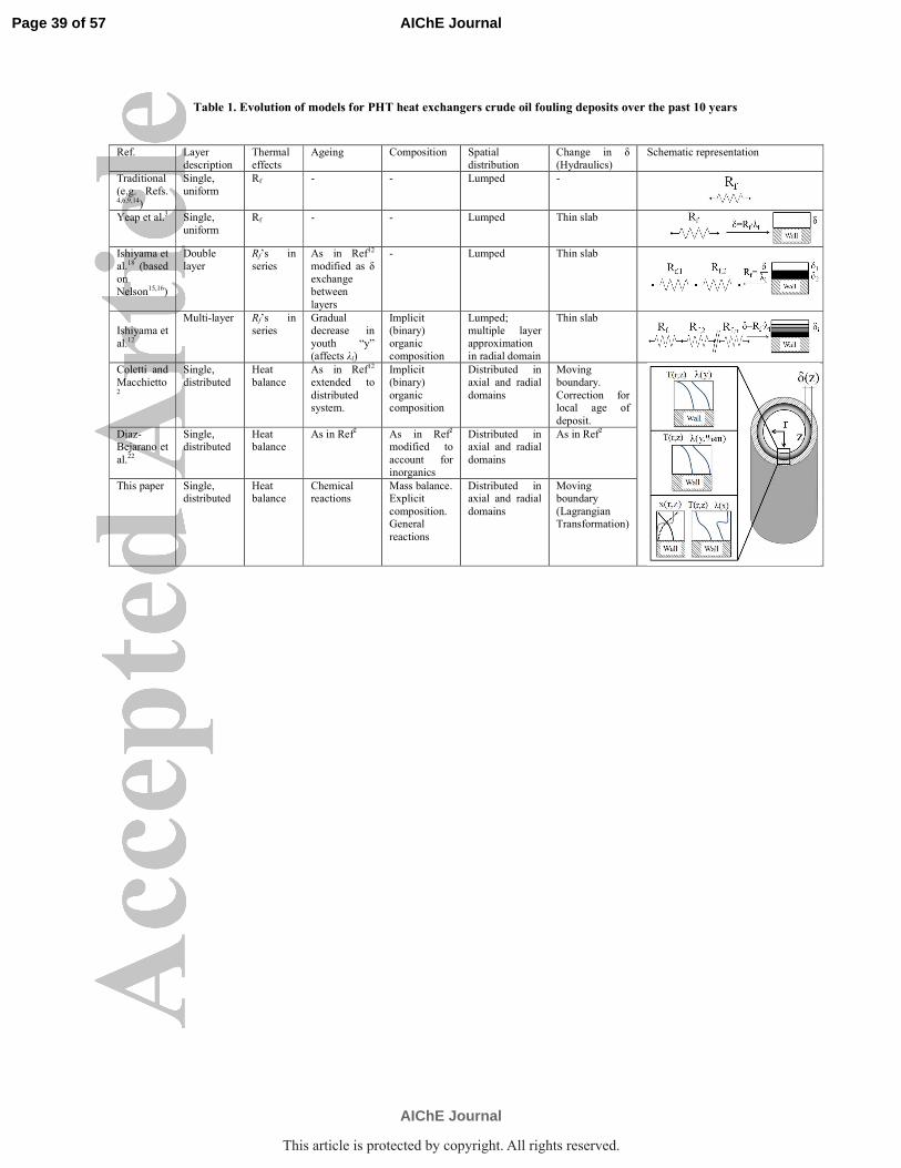
Table 1. Evolution of models for PHT heat exchangers crude oil fouling deposits over the past 10 years

Ref. Layer

description

Thermal

effects

Ageing Composition Spatial

distribution

Change in δ

(Hydraulics)

Schematic representation

Traditional

(e.g. Refs. 4,6,9,14)

Single,

uniform

Rf -

- Lumped -

Yeap et al.3 Single,

uniform

Rf - - Lumped Thin slab

Ishiyama et

al.18 (based

on

Nelson15,16)

Double

layer

Rf’s in

series

As in Ref12

modified as δ

exchange

between

layers

- Lumped Thin slab

Ishiyama et

al.12

Multi-layer Rf’s in

series

Gradual

decrease in

youth “y”

(affects λl)

Implicit

(binary)

organic

composition

Lumped;

multiple layer

approximation

in radial domain

Thin slab

Coletti and

Macchietto2

Single,

distributed

Heat

balance

As in Ref12

extended to

distributed system.

Implicit

(binary)

organic composition

Distributed in

axial and radial

domains

Moving

boundary.

Correction for local age of

deposit.

Diaz-Bejarano et

al.22

Single, distributed

Heat balance

As in Ref2 As in Ref2 modified to

account for

inorganics

Distributed in axial and radial

domains

As in Ref2

This paper Single, distributed

Heat balance

Chemical reactions

Mass balance. Explicit

composition. General

reactions

Distributed in axial and radial

domains

Moving boundary

(Lagrangian Transformation)

Page 39 of 57

AIChE Journal

AIChE Journal


Table 2. Parameters for single tube geometry, operating conditions, crude oil and fouling/cleaning models

Parameter value Parameter value

Tube Oil Physical Prop.

RI (mm) 9.93 API 37

RO (mm) 12.70 MeABP (ºC) 350

L (m) 6.1 ν38ºC (mm2s-1) 4

Operating conditions Fouling

UWT (ºC) 270 α' (kg m-2 s-1) 0.54

Tin (ºC) 200 γ' (kg m-2s-1Pa-1) 3.45· 10-9

Flowrate (kg/s) 0.3 Ef (kJ mol-1) 28

Cleaning Ageing

xC1,coke 0.5 Ea (kJ mol-1) 50

kC1 (kg/m2s) 3.2·10-4 Aa (s-1) (fast) 0.01

tC1 (days) 1 λgel (W m-1 K-1) 0.2

kM (kg/m3s) 0.027 λcoke (W m-1 K-1) 1.0

tM (days) 5

Page 40 of 57

AIChE Journal

AIChE Journal


Table 3. Comparison of key performance indicators for different timings of the chemical cleaning

Time of Chemical

Cleaning (month) 3 6 9 6 6

Type of Cleaning C1 C1 C1 C2 C3

δl,B - δl,C (mm) 0.48 0.56 0.58 0.34 0.81

(δl,B - δl,C)/δl,B (%) 74.2 47.0 35.0 29.0 68.0

(QC - QB)/Q0 (%) 44.4 25.1 16.9 14.6 40.2

(∆PB-∆PC)/∆P0 (%) 30.4 47.7 67.5 31.4 64.2

Comparison of performance C vs. A (δl,A = δl,C = 0.63 mm)

(q”C – q”A)/q”A (%) 36.4 51.0 47.6

(nf,C – nf,A)/nf,A (%) 13.1 10.9 7.9

Time after C to return to performance at B

Time for q” = q"B

(days) 75 108 130

Time for δl = δl,B (days)

69.3 92.5 107.8

Page 41 of 57

AIChE Journal

AIChE Journal


Figure 1. Schematic representation of the model for a single tube. 144x123mm (300 x 300 DPI)

Page 42 of 57

AIChE Journal

AIChE Journal


Figure 2. Schematic representation of fouling layer growing between times t1 (left) and t2 (right) undergoing reactions, in dimensional coordinates (a) and equivalent layer after Lagrangian transformation

(b). 204x162mm (300 x 300 DPI)

Page 43 of 57

AIChE Journal

AIChE Journal


Figure 3. Schematic representation of complete (a) and partial (b) cleaning of a fouling deposit undergoing ageing.

234x137mm (300 x 300 DPI)

Page 44 of 57

AIChE Journal

AIChE Journal


Figure 4. Deposit thickness reduction for fixed time (a) and condition-based (b) cleaning. The vertical lines indicate the start and end of the cleaning period.

250x106mm (300 x 300 DPI)

Page 45 of 57

AIChE Journal

AIChE Journal


Figure 5. Deposit thickness at the midpoint of the tube (z = 3.05m) over time with a chemical cleaning after 6 months.

130x88mm (300 x 300 DPI)

Page 46 of 57

AIChE Journal

AIChE Journal


Figure 6. Thickness and radial (dimensional) concentration profiles at the tube midpoint (z = 3.05m), at key times in periods i, ii and iii (left to right).

569x312mm (300 x 300 DPI)

Page 47 of 57

AIChE Journal

AIChE Journal


Figure 7. Fouling layer temperature profile at the tube midpoint (z=3,05m) at various times. 186x152mm (300 x 300 DPI)

Page 48 of 57

AIChE Journal

AIChE Journal


Figure 8. Volume fraction of gel at the deposit layer surface in the tube midpoint during periods i, ii and iii. 96x58mm (300 x 300 DPI)

Page 49 of 57

AIChE Journal

AIChE Journal


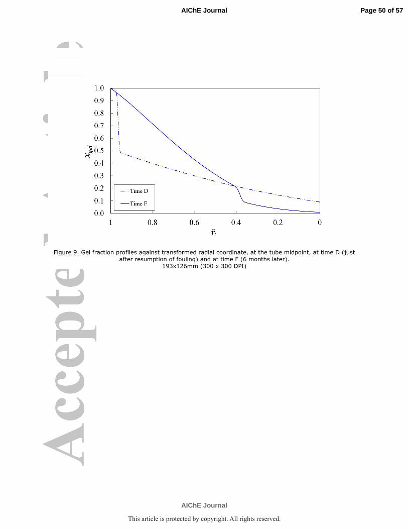
Figure 9. Gel fraction profiles against transformed radial coordinate, at the tube midpoint, at time D (just after resumption of fouling) and at time F (6 months later).

193x126mm (300 x 300 DPI)

Page 50 of 57

AIChE Journal

AIChE Journal


Figure 10. Deposit thickness at the tube midpoint (z= 3.05m) (a),Heat duty (normalized to clean duty) (b) and Thermo-hydraulic performance (c) for a single chemical cleaning C1 after 3, 6 and 9 months and

cleanings C2, C3 after 6 months.

144x266mm (300 x 300 DPI)

Page 51 of 57

AIChE Journal

AIChE Journal


Figure 11. Volume fraction of coke as function of the radial coordinate (dimensionless) and time at the tube midpoint (z = 3.05m) for a year without cleaning. The shaded area indicates the non-removable portion by

chemical cleaning C1. 150x123mm (300 x 300 DPI)

Page 52 of 57

AIChE Journal

AIChE Journal


Figure 12. Deposit thickness at the tube midpoint (z= 3.05m) (a) and heat duty (b) over time for operation during 450 days with condition-based chemical (C1) and fixed-time mechanical cleanings.

134x246mm (300 x 300 DPI)

Page 53 of 57

AIChE Journal

AIChE Journal


Figure 13. Effect of ξ on gel volume fraction at the surface of the layer during period (ii) and beginning of (iii) (re-start)

119x71mm (300 x 300 DPI)

Page 54 of 57

AIChE Journal

AIChE Journal


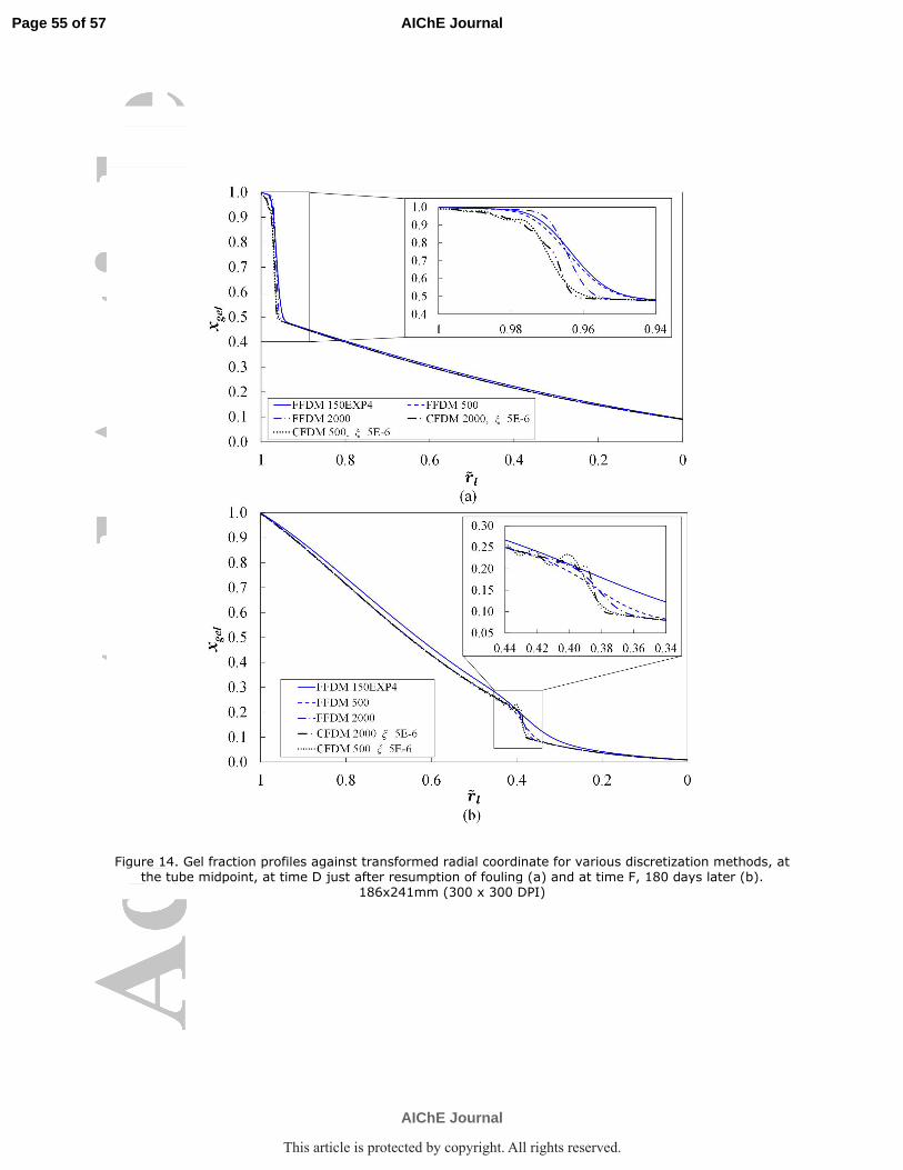
Figure 14. Gel fraction profiles against transformed radial coordinate for various discretization methods, at the tube midpoint, at time D just after resumption of fouling (a) and at time F, 180 days later (b).

186x241mm (300 x 300 DPI)

Page 55 of 57

AIChE Journal

AIChE Journal


Figure 15. Comparison of models I and II for fouling build-up for 3 values of γ’ over a year of operation at the tube midpoint (z=3.05): (a) deposit thickness and impact on heat flux (in the inside); (b) concentration

radial profile after a year.

422x584mm (300 x 300 DPI)

Page 56 of 57

AIChE Journal

AIChE Journal


Figure 16. Comparison of models I and II at the tube midpoint (z=3.05) for fouling build up with mechanical cleaning after 6 months: (a) deposit thickness; (b) concentration radial profile at times B’, C’ and E’.

420x566mm (300 x 300 DPI)

Page 57 of 57

AIChE Journal

AIChE Journal


Documents

A new dynamic model of crude oil fouling deposits and its ... et al... · time. The most widely used models to quantify crude oil fouling in refineries are the semi-empirical “threshold”