HAL Id: hal-02134750https://hal.archives-ouvertes.fr/hal-02134750

Submitted on 20 May 2019

HAL is a multi-disciplinary open accessarchive for the deposit and dissemination of sci-entific research documents, whether they are pub-lished or not. The documents may come fromteaching and research institutions in France orabroad, or from public or private research centers.

L’archive ouverte pluridisciplinaire HAL, estdestinée au dépôt et à la diffusion de documentsscientifiques de niveau recherche, publiés ou non,émanant des établissements d’enseignement et derecherche français ou étrangers, des laboratoirespublics ou privés.

A new dynamic predictive maintenance framework usingdeep learning for failure prognostics

Thi Phuong Khanh Nguyen, Kamal Medjaher

To cite this version:Thi Phuong Khanh Nguyen, Kamal Medjaher. A new dynamic predictive maintenance frameworkusing deep learning for failure prognostics. Reliability Engineering and System Safety, Elsevier, 2019,188, pp.251-262. �10.1016/j.ress.2019.03.018�. �hal-02134750�

Open Archive Toulouse Archive Ouverte (OATAO) OATAO is an open access repository that collects the work of some Toulouse

researchers and makes it freely available over the web where possible.

This is an author's version published in: https://oatao.univ-toulouse.fr/23365

Official URL : https://doi.org/10.1016/j.ress.2019.03.018

To cite this version :

Any correspondence concerning this service should be sent to the repository administrator:

tech-oatao@listes-diff.inp-toulouse.fr

Nguyen, Thi Phuong Khanh and Medjaher, Kamal A new dynamic predictive maintenance framework using deep learning for failure prognostics. (2019) Reliability Engineering and System Safety, 188. 251-262. ISSN 0951-8320

OATAO Open Archive Toulouse Archive Ouverte

A new dynamic predictive maintenance framework using deep learning forfailure prognosticsKhanh T.P. Nguyen⁎, Kamal MedjaherLGP, ENIT, Toulouse INP, 47 Avenue dʼAzereix, BP 1629 - 65016, Tarbes Cedex, France

Keywords:PHMPrognostics informationResidual life predictionPredictive maintenanceDeep learningInventory management

A B S T R A C T

In Prognostic Health and Management (PHM) literature, the predictive maintenance studies can be classifiedinto two groups. The first group focuses on the prognostics step but does not consider the maintenance decisions.The second group addresses the maintenance optimization question based on the assumptions that the prog-nostics information or the degradation models of the system are already known. However, none of the twogroups provides a complete framework (from data-driven prognostics to maintenance decisions) investigatingthe impact of the imperfect prognostics on maintenance decision. Therefore, this paper aims to fill this gap ofliterature. It presents a novel dynamic predicive maintenance framework based on sensor measurements. In thisframework, the prognostics step, based on the Long Short-Term Memory network, is oriented towards the re-quirements of operation planners. It provides the probabilities that the system can fail in different time horizonsto decide the moment for preparing and performing maintenance activities. The proposed framework is vali-dated on a real application case study. Its performance is highlighted when compared with two benchmarkmaintenance policies: classical periodic and ideal predicted maintenance. In addition, the impact of the im-perfect prognostics information on maintenance decisions is discussed in this paper.

1. Introduction

Due to the increasing requirement of reliability, availability,maintainability and safety of systems, the traditional maintenancestrategies are becoming less effective and obsolete. Beside, the revolu-tion of Industry 4.0 provides more convenient supports for the widedevelopment of the predictive maintenance (PdM) in practice. For ex-ample, the use of intelligent sensors provides a reliable solution forsystem monitoring in real time. Having this information, the managercan plan the maintenance activities more effectively to reduce machinedowntimes and improve the production flow.

According to this rising practical requirement, the PdM has alsoreceived significant attention in literature over the last decade, see[1–3] for recent overviews. Generally, the predicted maintenance fra-mework consists of two connected key parts: prediction of the systemresidual useful life time (RUL) and making decisions. Based on theprognostics approaches, the studies can be classified in two maingroups: model based and data-driven based PdM framework.

The first PdM group relies on stochastically modeling the systemdegradation evolution in the discrete or continuous time. The discretemodeling can be based on the Markov process and its variants for whichthe transition probabilities of system states are assumed to be known

with the historical reliability data [4–7]. Beside, the continuous mod-eling is built on the assumption that there exits a stochastic processcharacterizing the degradation mechanism of the system [8–10].Therefore, the performance of the PdM frameworks in this group de-pends on the prior knowledge quality of system degradation processes.From a theoretical view, it is very difficult to formalize or model a realdeterioration mechanism of a complex system. From a practical view,even if a theoretical model is built, it can not be directly applied inindustry where there exists various operation variables, e.g.loads overtime can affect the validity of the proposed model. A simplification ofthe system real working conditions can lead to wrong maintenancedecisions. To overcome these issues, the data-driven PdM frameworkhas been developed.

In the second group, data-driven PdM framework uses sufficientdata to predict the system RUL without knowing the physical nature ofthe degradation mechanism [11–14]. Its performance strictly dependson signal processing and feature engineering techniques. The tradi-tional data-driven approaches [15–17] require manual processing andanalysis of data by human experts and this might not be suitable for thecase of big data where an automatic process is preferable [18].Therefore, in recent studies, the deep learning (DL) methods becomeone of the most popular trends in data-driven diagnostic and

⁎ Corresponding author.E-mail addresses: thi-phuong-khanh.nguyen@enit.fr (K.T.P. Nguyen), kamal.medjaher@enit.fr (K. Medjaher).

prognostics that allows automatically extracting and constructing the useful information without the expertise knowledge of signal proces­sing. For example, an effective multi-sensor health diagnostic method using a deep belief network classifier was presented in [19]. A combi­nation between deep Boltzmann machines and a random forest was proposed in [20] to improve fault diagnostic performance for gearboxes by using acoustic and vibration signals. For recent studies, the article [21] developed an integrated hierarchical learning framework to per­form both diagnostics and prognostics. In papers [22,23], the authors proposed to use the Long Short-Term Memory (LSTM) network, which is an architecture specialized in discovering the underlying time series patterns to predict the system RUL. In [24], a new deep neural network structure named Convolutional Bi-directional Long Short-Term Memory networks (CBLSTM) was designed to address raw sensory data for RUL prediction. In [25], a Restricted Boltzmann machine (RBM) was used as an unsupervised pre-training stage to learn abstract features for the LSTM input in a supervised RUL regression stage. The LSTM was also applied for the RUL prediction problem of proton exchange membrane fuel cell (PEMFC) [26,27]. In detail, the work proposed in [26] used the regular interval sampling and locally weighted scatterplot smoothing (LOESS) for data reconstruction. Then, the smoothing data is fed into a LSTM network to predict the RUL value. On the other hand, in [27], the authors developed a two-dimensional (2D) grid LSTM to optimize the prediction accuracy of the fuel cell performance degradation.

The above mentioned studies in the data-driven prognostics group only focus on the prognostics step and do not consider the maintenance decisions, which are covered separately. For example, the papers [28,29] addressed the post-prognostics issue but based on the as­sumption that the prognostics information of the system are already known. In [30], the authors developed a model that allows evaluating the failure probability of a furnace component and then, based on it, deciding the replacement time. However, by considering the prog­nostics aspect, their contribution belongs to the group of model-based approaches, i.e. the data are only used for model parameter estimation and not for model construction. Hence, it inherits some drawbacks of the model-based prognostics approaches, such as the requirement of expert knowledge to construct the model. Moreover, the developed model is application-specific and cannot be implemented in different physical systems. Finally, considering the maintenance decision for­mulation, the performance of the model presented in [30] strictly de­pends on the failure threshold definition that is not trivial in practice.

Therefore, it is necessary to propose a new framework that satisfies the following requirements: 1) the prognostics approach can be widely implemented for various systems, even complex ones; 2) the dynamic and flexible m aintenance d ecision model s hould allow considering multiple options and evaluating rapidly their costs in order to make an instantaneous decision. This paper aims to address these requirements. The main contribution is to propose a new dynamic predictive main­tenance framework from the point of view of operation planners. To our humble knowledge, this is the first paper that considers a complete process from data-driven prognostics to maintenance decision. It allows providing the system failure probabilities in different time windows and also making an instantaneous maintenance/ inventory decision based on this prognostic information. In detail, we propose to use the LSTM network to estimate the probabilities that the system will fail in

Monitoring system with

muhiple sensors

Historical ~ - d_a_ta_ ~ Training LSTM

classier

Current data (on-line)

different time windows in the future. Although the LSTM network has been developed and improved in PHM literature, the previous studies [22-27] are based on a piece-wise linear (PWL) RUL target function, in which it is not trivial to define the RUL maximum value. Moreover, in these studies, the prognostics is treated as a regression problem. It only provides a predicted RUL value, whose the accuracy strictly depends on the prediction horizon, Le. the period starting from the current time (prediction instant) to the real system failure time. Therefore, using the predicted RUL value at the first stage of the system lifetime can lead to a wrong decision. Contrary to these studies, the prognostics method proposed in this paper does not require the PWL assumption and allows providing the probabilities that the system will fall into different time intervals. As these time intervals are defined according to the require­ments of the operation planner, the proposed method is expected to better adapt to practical demands. Moreover, its outputs do not depend on the period starting from the instant where the prediction is made to the real system failure time and then allows limiting the wrong deci­sions at the first-lifetime stage. Next, using these prognostics informa­tion, the proposed PdM framework allows providing the reasonable decisions to avoid the system failure, maximizing the system life time and reducing the inventory cost.

The remainder of paper is structured as follows. In Section 2, the Dynamic Predictive Maintenance (DPM) framework will be presented. The algorithm for evaluating the mean cost rate of the DPM framework and two benchmark policies will be developed in Section 3. In Section 4, the DPM framework will be verified on a real application case study: the turbofan engines. Its performance will be highlighted by comparing it with the classical periodic and the ideal predicted main­tenance policies. The impact of the imperfect prognostics information on the decisions and, consequently, on the performance of the proposed DPM will be also investigated in the same section. Finally, the con­clusion and further works will be discussed in Section 5.

2. New dynamic predictive maintenance framework

In practice, the prognostics information is usually required for a Jong horizon to plan different operation activities (e.g. maintenance, production or inventory, etc). Moreover, due to technological and lo­gistic constraints, the maintenance actions cannot be performed at every time and everywhere. As an illustration, the maintenance activ­ities for train or airplane engines cannot be realized during their journey. Hence, operation planners require the information whether the system fails in the determined time periods. For example, in the next week and the next month, what are the corresponding probabilities of the system failure? And then, how the maintenance decisions are made based on these prognostics information?

To answer the previous questions, this section aims to develop a new dynamic predictive maintenance framework that contains the total process from performing the prognostics based on multiple sensor measurements to making maintenance decisions, see Fig. 1. First, the prognostic method that provides the failure probability in different time windows will be developed in Section 2.1. Then, the decision rules taking into account spare-part-order option will be presented in Section 2.2.

LSTM network

Probabilities of Making decisions: r--s-ys""t_e_m._.a""'1,..u""'re ...... 1n~ Maintenance?

different time Order spare parts?

windows in future

Fig. 1. Dynamic predictive maintenance process.

Hidden er

2nd Hidden layer

LSTM layer Dropout layer

2nd unit nth unit 1st unit

1t;i' 1WBr · rtt+i' • ••• , C

• -- • .. Input ~ .,,,Output ~ 0 ,,. "

30 Tensor I \ ~

n2 hidden units Dropoot A Dropout D Dense layer

( softmax activation)

t •• •••• 1 st Hidden layer I I

No. of samples LSTM layer Dropout layer

2nd unit nth unit 1st unit

No. of classes

~~•11 ~r ~ t • •••> C + · J -- • · 1 ~ Input ~ _.,Output

\ v-' 0 -I I

I n1 hidden untts I Dropo<JI A Oropoul O

- -

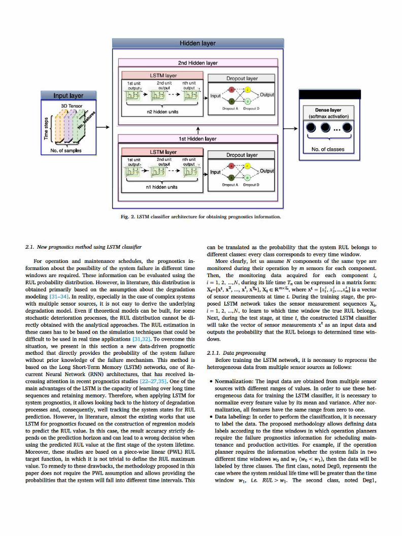
Fig. 2. LSTM classifier architecture for obtaining prognostics information,

2.1. New prognostics method using ISTM classifier

For operation and maintenance schedules, the prognostics in­formation about the possibility of the system failure in different time windows are required. These information can be evaluated using the RUL probability distribution. However, in literature, this distribution is obtained primarily based on the assumption about the degradation modeling [31- 34]. In reality, especially in the case of complex systems with multiple sensor sources, it is not easy to derive the underlying degradation model. Even if theoretical models can be built, for some stochastic deterioration processes, the RUL distribution cannot be di­rectly obtained with the analytical approaches. The RUL estimation in these cases has to be based on the simulation techniques that could be difficult to be used in real time applications [31,32]. To overcome this situation, we present in this section a new data-driven prognostic method that directly provides the probability of the system failure without prior knowledge of the failure mechanism. This method is based on the Long Short-Term Memory (LSTM) networks, one of Re­current Neural Network (RNN) architectures, that has received in­creasing attention in recent prognostics studies [22-27,35]. One of the main advantages of the LSTM is the capacity of learning over Jong time sequences and retaining memory. Therefore, when applying LSTM for system prognostics, it allows looking back to the history of degradation processes and, consequently, well tracking the system states for RUL prediction. However, in literature, almost the existing works that use LSTM for prognostics focused on the construction of regression models to predict the RUL value. In this case, the result accuracy strictly de­pends on the prediction horizon and can lead to a wrong decision when using the predicted RUL value at the first stage of the system lifetime. Moreover, these studies are based on a piece-wise linear (PWL) RUL target function, in which it is not trivial to define the RUL maximum value. To remedy to these drawbacks, the methodology proposed in this paper does not require the PWL assumption and allows providing the probabilities that the system will fall into different time intervals. This

can be translated as the probability that the system RUL belongs to different classes: every class corresponds to every time window.

More clearly, Jet us assume N components of the same type are monitored during their operation by m sensors for each component. Then, the monitoring data acquired for each component i,

i = 1, 2, .. . ,N, during its life time Tn can be expressed in a matrix form: X1= [x1, x2, .. . , xt, xTn], X1 e IRm"r", where x1 = [x:, x4, ... ,x~] is a vector of sensor measurements at time t. During the training stage, the pro­posed LSTM network takes the sensor measurement sequences XiJ i = 1, 2, .. . ,N, to learn to which time window the true RUL belongs. Next, during the test stage, at time t, the constructed LSTM classifier will take the vector of sensor measurements x1 as an input data and outputs the probability that the RUL belongs to determined time win­dows.

2.1.1. Data preprocessing Before training the LSTM network, it is necessary to reprocess the

heterogeneous data from multiple sensor sources as follows:

• Normalization: The input data are obtained from multiple sensor sources with different ranges of values. In order to use these het­erogeneous data for training the LSTM classifier, it is necessary to normalize every feature value by its mean and variance. After nor­malization, all features have the same range from zero to one.

• Data Jabeling: In order to perform the classification, it is necessary to label the data. The proposed methodology allows defining data labels according to the time windows in which operation planners require the failure prognostics information for scheduling main­tenance and production activities. For example, if the operation planner requires the information whether the system fails in two different time windows w0 and w1 (w0 < w1), then the data will be Jabeled by three classes. The first class, noted Deg0, represents the case where the system residual life time will be greater than the time window w1, i.e. RUL > w 1• The second class, noted Degl,

characterizes the case where the system residual life time is esti-mated in the period [w0, w1], i.e. w0≤ RUL<w1. Finally, the thirdclass, noted Deg2, concerns the case where the system residual lifewill not exceed the time window w0, i.e. RUL≤w0. Considering ncclasses, the classification output is a 1D array of nc elements. If thetrue RUL belongs to a given class, its corresponding element will beset to one while the remaining elements of the output array are setto zero. Note that in this paper, we will consider three classes.However the number of classes or time windows can be easily ex-tended when necessary.• Formalization: The LSTM input layer requires 3D tensor (see Fig. 2)for training the models and making predictions. Indeed, for timeseries data, it is necessary to format the input data as a 3D arraywith three dimensions: sample (ns), time step (nt), and feature (nf),see [36]. To identify nf, the different features can be extracted froma sensor output by numerous methods developed in literature, see abrief review in [37]. On the other hand, the sensor signals can bedirectly used to feed the LSTM input. For the case study presented inthis paper, one sensor output is considered as one feature. Next, theshape of the time step axis (nt) corresponds to the length of timesequence, which can be looked back by LSTM network when fittingmodels and predicting the output. Finally, considering ns, a sampleis a 2D array (nt, nf) that presents a time sequence of features. Forinstance, by monitoring the system during 100 hours with 21 sen-sors, and if the sensor outputs are directly used as inputs to theLSTM, then the number of features is 21 because each sensor outputis considered as a feature. Next, if the data are recorded once perhour and the sequence length of LSTM is chosen to be 30, thenumber of samples is: = + =n 100 30 1 71s . This means that thedata can be translated to a 3D tensor of shape ( =n 71,s =n 30,t

=n 21f ). Note that the first sample is a 2D array having 30 rows(from the first time step until the 30-th time step) and 21 columns(corresponding to 21 sensor measurements).

2.1.2. LSTM Classifier architectureA LSTM network is a recurrent neural network that allows addres-

sing the vanishing gradient problem caused by the repeated use of re-current weight matrix. It includes the LSTM cell blocks that containdifferent components called the input gate, the forget gate and theoutput gate. The details of LSTM cell block and its relevant mathema-tical functions were explained in previous studies [22,23,35]. In thispaper, the LSTM network is implemented for classification, and can becalled as LSTM classifier. Hence, the terms LSTM network and LSTMclassifier can be merged hereafter. This section aims to describe thearchitecture and configuration of the proposed classifier for the systemfailure prognostics.

The LSTM classifier proposed in this paper is constructed by usingthe python deep learning library, Keras. Fig. 2 shows its architecturethat has three types of layers: the input, the hidden and the outputlayers.

The input layer is a prototype bringing the data into the network forfurther processing. It requires 3D tensor with the following shape:number of samples, number of time steps and number of features.

Next, the hidden layer is the principal part of the network. It seeksto construct the relation between the input and the output. It cancontain one single or multiple layers. In this paper, two LSTM layers aresequentially stacked into the hidden layer. For LSTM configuration, thenumber of memory units for every layer have to be provided. It is ne-cessary to specify that the LSTM units return all of the outputs from theunrolled LSTM units through time. Then, it allows learning sequences ofobservations and it is well adapted to time series problem. However, itcan easily over-fit training data. Therefore, the “Dropout” regulariza-tion method is used for every LSTM layer to improve the model

performance. In Keras library, the “Dropout” is defined by the prob-ability that a unit can be excluded from the network. In detail, for eachtraining case in a mini-batch, by dropping out units, a thinned networkis sampled and its weights are evaluated [38]. Therefore, each hiddenunit in a network trained with dropout can learn how to work withrandomly chosen other units to create useful features. This should makeeach unit more robust and drive the network towards a generalizationto prevent the over-fitting.

Finally, the output layer contains a feed-forward neural networkthat is a regular fully connected layer. This layer is used as a prototypebetween the network and the output. It allows transforming the 3Dtensor at the hidden layer output to 1D array at the classifier output. Inthis paper, the classifier output is defined as a vector of 3 elementscharacterizing the probability that an observation belongs to 3 classes:Deg0, Deg1, and Deg2. Then, there are 3 units in the output layer andthe “softmax” activation function is proposed to be used. The outputlayer provides the probability distribution over the three classes (Deg0,Deg1, and Deg2).

For training the LSTM classifier, it is necessary to define the ob-jective function as “caterogical_crossentropy” that is specially used tosolve the multiple mutually-exclusive class problem. This function re-turns the cross-entropy H(p, q) between a predicted probability dis-tribution (p(x)) and a true probability distribution (q(x)). It is given by:

=H p q q x p x( , ) ( )log( ( ))x (1)

Next, for the optimization algorithm, we propose to use ADAM [39],which is an extension to stochastic gradient descent. This algorithm iswidely used for deep learning applications thanks to its efficient com-putation, the little memory requirement, and the suitability for pro-blems of large data and/or parameters.

For evaluating the performance of the model, the metric function isdefined as “categorical_accuracy”. Similar to the objective function, itprovides the mean accuracy rate across all predictions for multi-classclassification problems. However, its results are not used when trainingthe model.

2.1.3. Probability confusion matrixThis section aims to present a metric to evaluate the effectiveness of

the proposed LSTM classifier. In machine learning field, the confusionmatrix (M) is a popular way to evaluate the performance of the clas-sifier algorithm. As its rows represent the true labels (TL) and its col-umns characterize the predicted labels (PL), the diagonal elementsshow the numbers of correct labels for every class. In detail, the element(Mij) of this matrix represents the numbers of observations (x) whosethe predicted labels are j while the true labels are i. It is given by:

= = =M PL j TL iCount(( ) ( ));ij x x (2)

In this paper, we do not only predict to which class the observationbelongs, but provide the probability that it belongs to every class. Then,it is necessary to redefine the confusion matrix as the probability con-fusion matrix to evaluate the performance of the proposed algorithm.The element M̂ij of this matrix is the mean probability that the predictedvalue of an observation x is j while the true value is i. It is given by:

== =

=M

PL j TL iTL i

^ (( ) ( ))Count( )ij

x x x

x (3)

where = =PL j TL i(( ) ( ))x x is the probability that the predictedlabel of an observation x is j while its true label is i.

-~

n

L IP n

IP n

t.T P(RUL > w, )?

P(RUL$ wo)?

~ Preventive replacement

(non Out-o f-stock)

l!i.T ht.T+----+

L

(a) Update prognostics information (b) DN and order spare part (c) PR without out-of-stock

t,.T L

Corrective replacement (Out-of-stock)

t,.T

Corrective replacement (non Out-of-stock)

T.--+­l

(d) PR with out-of-stock (e) CR with out-of-stock (f) CR without out-of-stock

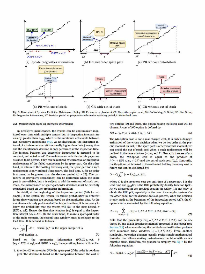
Fig. 3. Illustration of Dynamic Predictive Maintenance Policy. PR; Preventive replacement, CR: Corrective replacement, DN: Do Nothing, 0: Order, NO: Non Order, PI: Prognostics Information, ti.T: Decision period or prognostics information updating period, L: Order lead time.

2.2. Decision rules based on prognostic information

In predictive maintenance, the system can be continuously mon­itored over time with multiple sensors but its inspection intervals are usually greater than LimlD, which is the minimum achievable between two successive inspections [ 40]. As an illustration, the inspection in­terval of a train or an aircraft is normally higher than their journey time and the maintenance decision is only performed at the inspection time. The interval between two successive inspections is assumed to be constant, and noted as LiT. The maintenance activities in this paper are assumed to be perfect. They can be realized by corrective or preventive replacements of the failed component by its spare part. On the other hand, to minimize the holding inventory cost, the spare part for a such replacement is only ordered if necessary. The lead time, L, for an order is assumed to be greater than the decision period (L > .o.n. The cor­rective or preventive replacement can be performed when the spare part is unavailable, but it is subject to add the extra out-of-stock cost. Then, the maintenance or spare-part-order decisions must be carefully considered based on the prognostics information.

In detail, at the beginning of the inspection period (h-th for ex­ample), if the system still works, its failure probabilities in different future time windows are updated based on the monitoring data. As the maintenance is only performed at the inspection time, it is necessary to know the probability that the system will fail in the next period, P (RUL ,s; .o.n. Hence, the first time window (wo) is equal to the inspec­tion interval (w0 = t.T). On the other hand, to make a spare-part order at the right moment, the second time window must be relevant to the lead time. It is defined as follows:

W1 = [ ll.LT r •ll.T; where [xJ+ is the upper integer of a

real number x. (4)

Based on the prognostics information (P(RUL ,s; w0), P (w0 < RUL ,s; w1), and P(RUL > w1)), the operation planner will decide:

1. to order ( O) or no-order (NO) the spare part (if the order is not done yet). The decision is based on the comparison between the cost of

two options (O) and (NO). The option having the lower cost will be chosen. A cost of NO-option is defined by:

NO= Cos·P (w1 < RUL ::; w1 + ll.T) (5)

The NO-option cost is not a real charged cost. It is only a damage estimation of the wrong decision when we do not order at the pre­cise moment. In fact, if the spare part is ordered at that moment, we can avoid the out-of-stock cost when a such replacement will be realized in the time windows (wi, w1 + t.T ]. Hence, in the case of no­order, the NO-option cost is equal to the product of P(w1 < RUL ::; w1 + ll.T) and the out-of-stock cost (C05). Contrarily, the O-option cost is linked to the estimated holding inventory cost in future and can be evaluated by:

0 = C; J/0

(x - L)-!RUL (x)dx; (6)

where C1 is the inventory cost per unit time of a spare part, L is the lead time and fRuL(x) is the RUL probability density function (pdf). As we discussed in the previous section, in reality it is not easy to obtain the RUL pdf, especially in the case of a complex system. On the other hand, for the discrete decision process, when the decision is only made at the beginning of the inspection period (.o.n, the O­option can be evaluated by the following equation:

00

0 = C; L P((i - l )ll.T < RUL ::; i t.T)•(i t.T - W1)

i=lwiJt,.T(+ (7)

Note that the probability P((i - l)ll.T < RUL::; it.T ) can be ob­tained by the LS1M prognostic method proposed in this paper (see Section 2.1) when considering the multi-class classification problem with numerous time windows [(i - l )ll.T, it.T]. From another standpoint, operation planners usually prefer simple mathematical formulas that allows making instantaneous decision with an ac­ceptable error. Therefore, we propose to simplify the Eq. 7 by the following equation:

0 = P(RUL > W1)·C; [ max(fp - h~~ - Wi, tl.T) r ll.T (8)

Yes

Corrective maintenance

No

Continue to

Fig. 4. Algorithm for evaluating the DPM cost rate for a life cycle.

where h is the current period, and Tp is the mean time to failure of the system. In practice, Tp can be empirically obtained based on the historical reliability data of the system. Note that Eq. 8 is only an approximation of the holding inventory cost to make the decision rule simpler to be applied in reality. It is used for the real case study presented in this paper. Consequently, it is shown that the cost difference when using this expression is acceptable compared with the ideal case.

2. to replace (R) or do-nothing (DN). The decision is based on the comparison between the cost rate (cost part unit time) of two op­tions (R) and (DN): the option having the lower cost rate will be chosen. Their cost rates are given by:

R = Cp + Cos·O(Sh = 0) . ht.T

DN P(RUL < Wo)·(Cc + C;·O(Sh = l) t.T + Cos·O(Sh+i = 0))

(h + l ) t.T

(9)

(10)

In detail, given the current period h, if one decides to replace the degraded component, she/ he has to pay the preventive maintenance cost (Cp) and the out-of-stock cost (C05) linked to a spare part un­availability (Sh = 0). Then, the sum of these costs will be divided by the actual life time of the system (M1) to evaluate the cost rate. Contrarily, if the component is not preventively replaced, there exists the risk that it will fail in the next period (P(RUL s w0), with w0 = t.T ). In this case, the corrective maintenance will be per­formed with the cost Cc, which also includes the downtime cost, at the beginning of h + I period. Hence, its life time is equal to (h + l ) t.T. In addition, the holding inventory cost and the out-of­stock cost can be taken into account.

Fig. 3 illustrates the possible progress of the presented dynamic predictive maintenance policy. At the beginning of the inspection period, the probabilities that the system will fail in three time windows (P(RUL s w0), P(w0 < RUL s w1), and P(RUL > w1)) are updated. Based on these information, the appropriate options (R or DN, 0 or NO) will be chosen (see Sub-Fig. 3.(a)). Then, if at the moment MT we decide to do nothing and order the spare part, the system continues to work in the next period and the spare part is received after the lead time

L (see Sub-Fig. 3.(b)). For the next inspection period, as the order is done at MT, only the Rand DN options are evaluated. If the R option is

chosen after the moment ht.T + L, then the preventive replacement (PR) will be realized without the out-of-stock issue (see Sub-Fig. 3.(c)). Contrarily, the out-of-stock cost (Cos) have to be added in the main­tenance cost (see Sub-Fig. 3.(c)). In the case where the system is failed before a preventive maintenance, a corrective replacement (CR) will be performed at the beginning of the next period. If the spare part is un­available, the out-of-stock problem will occur (see Sub-Fig. 3.(d)) and vice-versa (see Sub-Fig. 3.(e)).

3. Performance evaluation of the proposed predictive maintenance framework

In order to highlight the performance of the proposed dynamic predictive maintenance framework (DPM), this section aims to present the algorithm for evaluating the DPM average cost rate. This result will be compared with the cost rates of the two following policies:

• Periodic maintenance policy (PeM) that is based on the historical reliability data of the system. In detail, using the historical relia­bility data, the mean time to failure Tp of the system is evaluated. Then, the periodic preventive maintenance with the cost Cp will be performed at the moment TR:

TR = [ :; rt.T (11)

As the maintenance activities have been planned in advance, the spare parts will be available at this moment. Contrarily, the spare part is unavailable for a corrective maintenance if the system is

failed before the moment TR, In this case, the corrective main­tenance cost Cc and the out-of-stock cost Cos will be added. Hence, the average cost rate of the Policy 2 is given by:

- 1 ~ Cp (Cos + Cc) cRP,M = - L.J - -o(TR > TR) +

1 1 1 o(TR < TR)

n i=l TR Tft t.T +,t,.T (12)

where n is the number of system life cycles, Ti;; is the failure time of the i-th life cycle and o(x ) is a direct function: o (x) = 1 when x is

true. • Ideal predicted maintenance policy (IPM) that is based on the

hypothesis of the perfect predicted failure time. In this case, at the inspection time, we assume that the residual life time is correctly determined. Then, the decisions based on this perfect information will minimize the cost rate value, which is given by:

- 1 ~ Cp CR1PM = - L.J

n i= l [(TR - 1)/t.TJ-•t.T (13)

where [x r is the lower integer of x. Thanks to the perfect prognostic information, the preventive maintenance will be performed with an available spare part at the moment [ (TR - 1)/t.Tt"•t.T which is the inspection time before the failure. Hence, the cost rate of i-th life cycle equals to the ratio between the preventive maintenance cost Cp

and the life cycle duration.

The algorithm for evaluating the cost rate of the proposed DPM policy is presented in Fig. 4. At the beginning of the i-th life cycle, the boolean variable Order and the state of the stock are set to zero. Without Joss of generality, considering the h-th inspection period for example, if the system is failed, the corrective replacement is performed. Other­wise, if the system still works but the R option is chosen, then the preventive replacement is realized. The proposed DPM cost rate is evaluated by Eq. 14.

Considering Eq. 14, if the system is failed, the corrective main-tenance will be performed with an available spare part when Sh>0.Contrarily, the out-of-stock cost (Cos) will be added if =S 0h . After thecorrective maintenance, the i-th life cycle is ended and a new life cycle

+i 1 will be started.However, when the system still works, the inventory state (char-

acterized by Sh and a boolean variable Order) and the prognostics in-formation PI (obtained by the LSTM classification, see sub-Section 2.1)will be updated. Based on these information, two decision branches willbe exploited.

On the first branch, the corresponding cost rates of the options Rand DN are evaluated by Eq. 10. If DN> R, a preventive maintenancewill be performed with the available spare part when Sh>0 while theCos will be added when =S 0h . Then, the i-th life cycle is ended and thecorresponding cost rate is calculated by Eq. 14. Otherwise, if DN> R,the system continues to work until the next inspection time.

On the second branch, if =Order 0, the corresponding cost rates ofthe options NO and O are evaluated by Eq. 5 and Eq. 8. Then, ifNO>O, the boolean variable Order and the state of stock after a leadtime will be set to one and we move to the next period. In the caseswhere =Order 1 or the NO option cost is less than the O-option cost, wedirectly consider the next period.

After evaluating the cost rate of n life cycles, the average cost rate ofthe DPM policy is given by:

=CRn

CR¯ 1DPM

i

n

i(15)

4. Real application case study

In this section, the proposed DPM is verified on the benchmarkingdata set: Turbofan Engine Degradation Simulation provided by NASAAmes Prognostics Data Repository. This data set is widely used in PHMfield, see [41] for a review of the prognostic studies using it. It isgenerated by C-MAPSS tool that simulates various degradation sce-narios of the fleet of engines of the same type. At the beginning of eachscenarios, the engine is normally operating. It is degraded until a failurein the training set. In the test set, the degradation process ends sometime prior to system failure. Both of training and test sets consist of 26columns that describe the characteristics of the engine units. The firstand second column respectively represent the ID and the degradation

time steps for every engine. The next three columns characterize theoperation modes of the engines while the final 21 columns correspondto the outputs of 21 sensors.

The C-MAPSS data set includes 4 subsets: FD001, FD002, FD003 andFD004, which correspond to 4 different cases combining different op-erating conditions and fault modes. The subsets FD001 and FD003 aresubject to a single operating condition while the subsets FD002 andFD004 present six operating conditions. Moreover, there exists only onefault mode in the subsets FD001 and FD002 while the subsets FD003and FD004 are more complex due to two failure modes. Table 1 sum-marizes the characteristics of the corresponding test sets. In this table,the statistical indicators (Min, Max, Mean, Median) of the recorded datalength of different turbofan engines are evaluated for every test set. Itcan be seen that the recorded data length are not uniform across eachset. For example, in the test set FD001, there are 100 trajectories.Among them, the minimum length and the maximum length are re-spectively 31 and 303. The mean and median values of the recordeddata lengths for this set are then respectively 130.96 and 133.5.

4.1. Discussion of prognostics accuracy

To construct the LSTM classifier presented in Section 2.1, the py-thon deep learning library Keras was used. The configuration para-meters are summarized in Table 2. For the formalization of the LSTMdata input, it is necessary to define the sequence length (nt). The valueof this parameter should be smaller than that one of the recorded datalength, i.e. the length of the recorded trajectories. In addition, thegreater value of nt is, the higher capacity of looking back in the historydata of the LSTM will be. However, this will lead to an increase of thetraining time. Therefore, for every test set in the case study, it is pre-ferable to have the values of nt enough large to benefit from the historyinformation, but must be smaller than the minimum length of the re-corded trajectories. Note that the minimum recorded lengths are 31 forFD001, 21 for FD002, 38 for FD003 and 19 for FD004, see Table 1.Then, the corresponding values nt are respectively chosen as follows: 30for FD001, 20 for FD002, 30 for FD003, and 10 for FD004.

As mentioned in the previous section, the prognostic method pro-posed in this paper provides the probability that the system will fail inthe different time windows in the future instead of a precise RUL value.Therefore, we cannot use the common evaluation criteria such asPHM08 score, MAE, MAPS, MSE to evaluate the performance of theproposed method and compare it with the published studies in litera-ture [42–44]. Instead, we propose to use the confusion probabilitymatrix presented in Section 2.1.3 to evaluate the accuracy of theprognostics information. It also provides the benchmark results forfurther studies for whom wants to focus on the improvement of theprognostic algorithms.

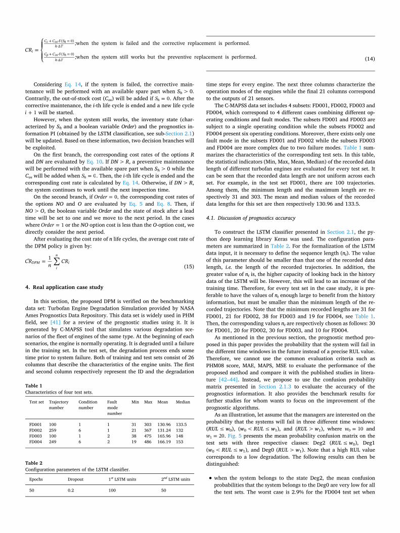
As an illustration, let assume that the managers are interested on theprobability that the systems will fail in three different time windows:(RUL≤w0), (w0< RUL≤w1), and (RUL>w1), where =w 100 and

=w 201 . Fig. 5 presents the mean probability confusion matrix on thetest sets with three respective classes: Deg2 (RUL≤w0), Deg1(w0< RUL≤w1), and Deg0 (RUL>w1). Note that a high RUL valuecorresponds to a low degradation. The following results can then bedistinguished:

• when the system belongs to the state Deg2, the mean confusionprobabilities that the system belongs to the Deg0 are very low for allthe test sets. The worst case is 2.9% for the FD004 test set when

Table 1Characteristics of four test sets.

Test set Trajectorynumber

Conditionnumber

Faultmodenumber

Min Max Mean Median

FD001 100 1 1 31 303 130.96 133.5FD002 259 6 1 21 367 131.24 132FD003 100 1 2 38 475 165.96 148FD004 249 6 2 19 486 166.19 153

Table 2Configuration parameters of the LSTM classifier.

Epochs Dropout 1st LSTM units 2nd LSTM units

50 0.2 100 50

=

+ =

+ =CR

;when the system is failed and the corrective replacement is performed.

;when the system still works but the preventive replacement is performed.i

C C Sh T

C C Sh T

· ( 0)·

· ( 0)·

c os h

p os h(14){ ;

considering 6 operating conditions and 2 failure modes. In the casesof the FD001 and FD003 test sets, when only one operating condi-tion is investigated, these probabilities are negligible and are ap-proximately equal to zero.• when the system is in the state Deg0, the mean confusion probabilityof the state Deg2 is also non-significant for all the test sets. Themaximum value is 3.4% in the case of FD003 test set where twofailure modes and one operating condition is considered.• when the system belongs to the state Deg1, its predicted state isnormally the state Deg2, especially in the case of FD001 and FD003test sets. However, this phenomenon can be explained by the factthat two time windows w0 and w1 are so close together. Hence, thecharacteristics of the systems that belong to the state Deg1 in thetest sets are similar to the ones of the state Deg2 in the training sets.Next, we will consider the change of the confusion probability ma-trix in different lengths of the time window w1.

Using the test set FD001, Fig. 6 shows the impact of time window w1

on the probability confusion matrix. It can be seen that the confusionprobabilities between the state Deg0 and the state Deg2 are negligible

for all 4 values of w1. On the other hand, the confusion probability thatthe predicted state is Deg2 when the true state is Deg1 is decreasing inw1. Contrarily, the confusion probabilities between the states Deg0 andDeg1 are increasing in w1. The confusion probabilities between thepredicted classes can be reduced by further studies on the optimizationof the LSTM architecture or on the configuration parameters. However,as mentioned in the previous section, this paper does not focus speci-fically on the development of the prognostics method. We are interestedon the use of the prognostics information for the predicted main-tenance. Therefore, instead of the improvement of the prognostics, wewill consider in the next section the impact of these confusions on theperformance of the proposed predicted maintenance policy.

4.2. Dynamic predictive maintenance framework

Next, the proposed DPM framework will be verified on the firstturbofan engine data set, FD001. In order to evaluate and compare theperformance of three maintenance policies (DPM, PeM and IPM) pre-sented in Section 3, the total information of the engines states during alltheir life cycles (from the beginning to the failure) are necessary.

Fig. 5. Probability confusion matrix (%) on test sets with =w 10,0 =w 201 . (Deg2: RUL≤w0, Deg1: w0< RUL≤w1, Deg0: RUL>w1). Note: a dark color corre-sponds to a high probability value.

Fig. 6. Probability confusion matrix (%) ontest set FD001 with different time window w1.(Deg0: RUL≤w0, Deg1: w0< RUL≤w1,Deg2: RUL>w1). Note: a dark color corre-sponds to a high probability value. (For inter-pretation of the references to colour in thisfigure legend, the reader is referred to the webversion of this article.)

Table 3Dynamic predictive maintenance scenarios, =C 100,p =C 500,c =C 0.1,i =C 10os (Deg2: RUL≤10, Deg1: 10< RUL≤20, Deg0: RUL>20).

Life time True RUL Deg0 (%) Deg1 (%) Deg2 (%) Order Stock Maintenance

Engine ID82 ( =T 214f )170 44 99.99 0.01 0 0 0 0180 34 99.91 0.09 0 0 0 0190 24 80.55 19.46 0.09 1 0 0200 14 0.02 76.96 23.02 1 0 0210 4 0 0 100 1 1 1

Engine ID81 ( =T 200f )180 60 99.78 0.21 0.01 0 0 0190 50 99.61 0.37 0.02 0 0 0200 40 78.86 21.02 0.11 1 0 0210 30 34.63 64.15 0.22 1 0 0220 20 0.37 93.62 6.01 1 1 0230 10 0.36 76.22 23.42 1 1 1

Engine ID83 ( =T 293f )250 43 99.95 0.05 0 0 0 0260 33 99.9 0.09 0.01 0 0 0270 23 4.06 95.76 0.18 1 0 0280 13 0.05 43.05 56.9 1 0 1

- VO - -Ji Ji Ji ~~1 0.00 .,. ~ De91 ~~l

1 ~ 1

""'' 000 0.02 ""'' ""'' ✓ # #' ✓ <I'~ #'

Predicted label Prflktedlaoel

(a) FD00l (b) FD002

(a) wo = 10, w, = 30 (b) wo = 10,w, = 50 (c) wo = 10, w, = 70

"'

000 017

000 005

✓ #' <P Predw:ted label

(c) FD003

(d) wo = 10, w, = 90

-Ji ~ "'91

1

I .. .. .. ,.

""''

rn .,

.. U!36 1751

.,

, .. .,, .,

✓ #' #' Prfedw:ted label

(d) FD004

~-- ----170

~-- -- --0 170

~------170

P(RUL > 20) = 99.91% P (IO < RUL $ 20) = 0.09%

P(RUL $10) •0%

(a) Cmrent time t = 180

L

Time

Time ~ jJJI

180 190 ""-------- 214 True

Failure P(RUL > 20) • 80.55% time P(IO < RUL $ 20) = 19.46% P(RUL 5 10) • 0-09%

(b) Current time t = 190

Sh • O, Order = 1

Time

True 180 190 214 Failure

P(RUL > 20) • OJ>2% P(IO < RUL 5 20) • 76.96%

time P(RUL5 l0)= 23.02%

(c) Current time t = 200

Spare part Sh e 1,

arrives in stock 0fder = 1

Time

True 180 214 Failure

P(RUL > 20) = O¾ time P(l O < RUL 5 20) = O¾

P(RUL $ 10) = 100%

(d) Current time t = 210

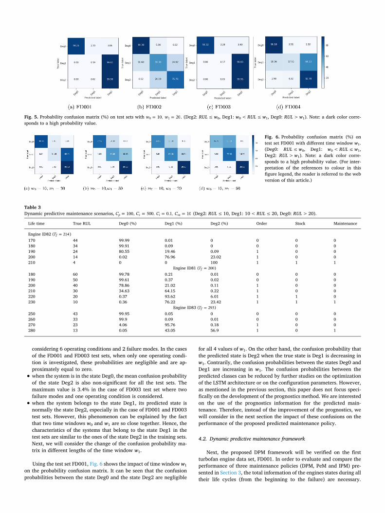
Fig. 7. Illustration of the maintenance/ inventory decisions at each time step for the engine 1082.

Table 4

Illustration of the flexibility of maintenance decisions.

ID r, Otlrne No. Stock period

Case A: Cp = 100, C, = 500, C; = 1, C., = 10

81 240 200 1

83 293 270 0 84 267 250 0 Case B: Cp = 100, C, = 200, C; = 0.1, C.,.. = 20 81 240 210 1 83 293 270 0 84 267 210 3

R time

230 280 260

240 290

260

00S

0

0 0

0

Hence, in this section, the FD00l training set will be divided into two parts. The first part, including 80 first trajectories, is used for training the lSIM while the second part, consisting of 20 remaining trajectories, is used for evaluating the performance of the DPM framework.

Given w0 = ti.T = 10, w1 = L = 20, at every inspection time h · l1T, where h E (1, 2, 3, .. . ], and based on the sensor measurements, the

I.S1M classifier provides the prognostics information of the engine for making maintenance decisions.

4.2.1. Optimal decisions of DPM Table 3 shows some last inspection periods of the life cycle of three

engines (ID 81, 82, 83) to illustrate how the DPM works. The two first columns present the lifetime and the true RUL of each engine, while the three next columns show respectively the probabilities that an engine belongs to the three classes: Deg0 (RUL > 20), Degl (10 < RUL ~ 20) and Deg2 (RUL < 10). The remaining columns (Order, Stock, and Maintenance) present the corresponding boolean variables which characterize the Order, the stock and the maintenance states, respec­tively.

Considering the engine ID82, one can see that at t = 180, the values in the three columns Order, Stock and Maintenance equal to zeros. That means before t = 180, the optimal decision is to do nothing (DN) and no order (NO). Fig. 7 illustrates the maintenance/inventory decisions for the engine ID82. From figure7(a), one can see that, at t = 180, i.e. at the beginning of the h-th decision period (h = 18), the engine still works, its

Cost ---------------rate

2S

20

JS

10

~ CR_OPM -t- CR_PeM ~ CR_IPM

0 _______________ _,

100 200 300 400 SOO 600 700 800 ,00 1000 Cp

(a) Cc = 10 · C,,, C, = 0.1, C0 , = 100

C<>st rate--.. - -- -- -- -- -- ... - -- -- -- -- ..... - ... - _- _- _- _- ... - -- _- _- _- _- ... --

10

.., M M Cl

~ CR_DPM ..... CR_Pet-1 ~ CR_IPM

.. (c) Cp = 500, Cc = 5000, c •• = 10 · C,

Cost ;:::::;:::::;;::::;::::;:::::;;::::;:::::;;::::;;:::~ rate

12

10

2

... CR_DPM -t- CR_PeM ~ CRJ PM

S U U ~ ~ ~ ~ ~ 0 ~ CoSIO

(b) C,, = 500, Cc = 5000, C, = 0.1

Cost rate 40 ..,. CR._OPM

..... CR._PeM l S ~ CR.J PM

30

2S

20

1S

10

10 1S k

20 2S 30

(d) k = Cc/Cp with Cp = 500, C •• = 100, C, = 0.1

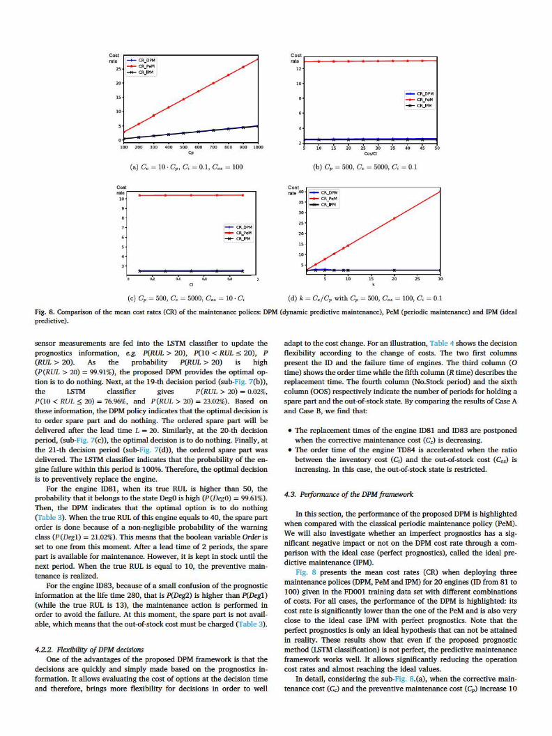
Fig. 8. Comparison of the mean cost rates (CR) of the maintenance polices: DPM (dynamic predictive maintenance), PeM (periodic maintenance) and IPM (ideal predictive).

sensor measurements are fed into the I.STM classifier to update the prognostics information, e.g. P(RUL > 20), P(lO < RUL :s; 20), P (RUL > 20). As the probability P(RUL > 20) is high (P(RUL > 20) = 99.91 %), the proposed DPM provides the optimal op­tion is to do nothing. Next, at the 19-th decision period (sub-Fig. 7(b)), the I.STM classifier gives P (RUL > 20) = 0.02%, P (lO < RUL ~ 20) = 76.96%, and P(RUL > 20) = 23.02%). Based on these information, the DPM policy indicates that the optimal decision is to order spare part and do nothing. The ordered spare part will be delivered after the lead time L = 20. Similarly, at the 20-th decision period, (sub-Fig. 7(c)), the optimal decision is to do nothing. Finally, at the 21-th decision period (sub-Fig. 7(d)), the ordered spare part was delivered. The lSfM classifier indicates that the probability of the en­gine failure within this period is 100%. Therefore, the optimal decision is to preventively replace the engine.

For the engine ID81, when its true RUL is higher than 50, the probability that it belongs to the state DegO is high (P(DegO) = 99.61%). Then, the DPM indicates that the optimal option is to do nothing (Table 3). When the true RUL of this engine equals to 40, the spare part order is done because of a non-negligible probability of the warning class (P(Degl ) = 21.02%). This means that the boolean variable Order is set to one from this moment. After a lead time of 2 periods, the spare part is available for maintenance. However, it is kept in stock until the next period. When the true RUL is equal to 10, the preventive main­tenance is realized.

For the engine ID83, because of a small confusion of the prognostic information at the life time 280, that is P(Deg2) is higher than P(Degl) (while the true RUL is 13), the maintenance action is performed in order to avoid the failure. At this moment, the spare part is not avail­able, which means that the out-of-stock cost must be charged (Table 3).

4.2.2. Flexibility of DPM decisions One of the advantages of the proposed DPM framework is that the

decisions are quickly and simply made based on the prognostics in­formation. It allows evaluating the cost of options at the decision time and therefore, brings more flexibility for decisions in order to well

adapt to the cost change. For an illustration, Table 4 shows the decision flexibility according to the change of costs. The two first columns present the ID and the failure time of engines. The third column (O time) shows the order time while the fifth column (R time) describes the replacement time. The fourth column (No.Stock period) and the sixth column (OOS) respectively indicate the number of periods for holding a spare part and the out-of-stock state. By comparing the results of Case A and Case B, we find that:

• The replacement times of the engine ID81 and ID83 are postponed when the corrective maintenance cost (CJ is decreasing.

• The order time of the engine TD84 is accelerated when the ratio between the inventory cost (Ci) and the out-of-stock cost (C0,) is increasing. In this case, the out-of-stock state is restricted.

4.3. Perfonnance of the DPM framework

In this section, the performance of the proposed DPM is highlighted when compared with the classical periodic maintenance policy (PeM). We will also investigate whether an imperfect prognostics has a sig­nificant negative impact or not on the DPM cost rate through a com­parison with the ideal case (perfect prognostics), called the ideal pre­dictive maintenance (1PM).

Fig. 8 presents the mean cost rates (CR) when deploying three maintenance polices (DPM, PeM and 1PM) for 20 engines (ID from 81 to 100) given in the FDOOl training data set with different combinations of costs. For all cases, the performance of the DPM is highlighted: its cost rate is significantly lower than the one of the PeM and is also very close to the ideal case 1PM with perfect prognostics. Note that the perfect prognostics is only an ideal hypothesis that can not be attained in reality. These results show that even if the proposed prognostic method (I.STM classification) is not perfect, the predictive maintenance framework works well. It allows significantly reducing the operation cost rates and almost reaching the ideal values.

In detail, considering the sub-Fig. 8.(a), when the corrective main­tenance cost (Cc) and the preventive maintenance cost (Cp) increase 10

0.25 "'I"'""-----------------------, -+- Cos/Ci = 100 -a- Cos/Ci = 300

0.20 -++- Cos/Ci = 500

0.15

0.10

0.05

0.00

0 20 40 60 80 100 Cc/Cp

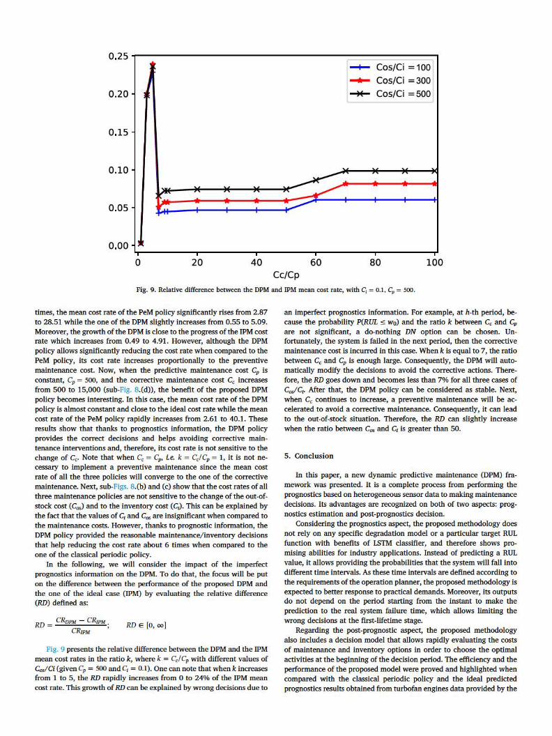
Fig. 9. Relative difference between the DPM and 1PM mean cost rate, with C, = 0.1, CP = 500.

times, the mean cost rate of the PeM policy significantly rises from 2.87 to 28.51 while the one of the DPM slightly increases from 0.55 to 5.09. Moreover, the growth of the DPM is close to the progress of the 1PM cost rate which increases from 0.49 to 4.91. However, although the DPM policy allows significantly reducing the cost rate when compared to the PeM policy, its cost rate increases proportionally to the preventive maintenance cost. Now, when the predictive maintenance cost Cp is constant, Cp = 500, and the corrective maintenance cost C, increases from 500 to 15,000 (sub-Fig. 8.(d)), the benefit of the proposed DPM policy becomes interesting. In this case, the mean cost rate of the DPM policy is almost constant and close to the ideal cost rate while the mean cost rate of the PeM policy rapidly increases from 2.61 to 40.1. These results show that thanks to prognostics information, the DPM policy provides the correct decisions and helps avoiding corrective main­tenance interventions and, therefore, its cost rate is not sensitive to the change of c,. Note that when Cc = Cp, i.e. k = CclCp = 1, it is not ne­cessary to implement a preventive maintenance since the mean cost rate of all the three policies will converge to the one of the corrective maintenance. Next, sub-Figs. 8.(b) and (c) show that the cost rates of all three maintenance policies are not sensitive to the change of the out-of­stock cost (Cos) and to the inventory cost (C,). This can be explained by the fact that the values of C1 and Cos are insignificant when compared to the maintenance costs. However, thanks to prognostic information, the DPM policy provided the reasonable maintenance/ inventory decisions that help reducing the cost rate about 6 times when compared to the one of the classical periodic policy.

In the following, we will consider the impact of the imperfect prognostics information on the DPM. To do that, the focus will be put on the difference between the performance of the proposed DPM and the one of the ideal case (1PM) by evaluating the relative difference (RD) defined as:

RD = CRvPM - CRrPM . CR1PM '

RD E [o, oo]

Fig. 9 presents the relative difference between the DPM and the 1PM mean cost rates in the ratio k , where k = Cc!Cp with different values of Cos/Ci (given Cp = SOO and q = 0.1). One can note that when k increases from 1 to 5, the RD rapidly increases from O to 24% of the 1PM mean cost rate. This growth of RD can be explained by wrong decisions due to

an imperfect prognostics information. For example, at h-th period, be­cause the probability P(RUL s wo) and the ratio k between C, and Cp are not significant, a do-nothing DN option can be chosen. Un­fortunately, the system is failed in the next period, then the corrective maintenance cost is incurred in this case. When k is equal to 7, the ratio between C, and Cp is enough large. Consequently, the DPM will auto­matically modify the decisions to avoid the corrective actions. There­fore, the RD goes down and becomes Jess than 7% for all three cases of CosfC1• After that, the DPM policy can be considered as stable. Next, when C, continues to increase, a preventive maintenance will be ac­celerated to avoid a corrective maintenance. Consequently, it can lead to the out-of-stock situation. Therefore, the RD can slightly increase when the ratio between Cos and C1 is greater than 50.

5. Conclusion

In this paper, a new dynamic predictive maintenance (DPM) fra­mework was presented. It is a complete process from performing the prognostics based on heterogeneous sensor data to making maintenance decisions. Its advantages are recognized on both of two aspects: prog­nostics estimation and post-prognostics decision.

Considering the prognostics aspect, the proposed methodology does not rely on any specific degradation model or a particular target RUL function with benefits of lSTM classifier, and therefore shows pro­mising abilities for industry applications. Instead of predicting a RUL value, it allows providing the probabilities that the system will fall into different time intervals. As these time intervals are defined according to the requirements of the operation planner, the proposed methodology is expected to better response to practical demands. Moreover, its outputs do not depend on the period starting from the instant to make the prediction to the real system failure time, which allows limiting the wrong decisions at the first-lifetime stage.

Regarding the post-prognostic aspect, the proposed methodology also includes a decision model that allows rapidly evaluating the costs of maintenance and inventory options in order to choose the optimal activities at the beginning of the decision period. The efficiency and the performance of the proposed model were proved and highlighted when compared with the classical periodic policy and the ideal predicted prognostics results obtained from turbofan engines data provided by the

[1] Snchez-Silva Mauricio, Frangopol Dan M., Padgett Jamie, Soliman Mohamed.Maintenance and operation of infrastructure systems: review. J Struct Eng2016;142(9).

[2] Wang K, Wang Y. How AI affects the future predictive maintenance: a primer ofdeep learning. 2018978-981-10-5767-0. p. 1–9.

[3] Gouriveau R, Medjaher K, Zerhouni N. From prognostics and health systems man-agement to predictive maintenance 1: monitoring and prognostics. 2016. https://doi.org/10.1002/9781119371052.

[4] Papakonstantinou K, Shinozuka M. Planning structural inspection and maintenancepolicies via dynamic programming and markov processes. part ii: pomdp im-plementation. Reliab Eng Syst Saf 2014;130:214–24.

[5] Papakonstantinou K, Shinozuka M. Planning structural inspection and maintenancepolicies via dynamic programming and markov processes. part i: theory. Reliab EngSyst Saf 2014;130:202–13.

[6] Nguyen TPK, Castanier B, Yeung TG. Maintaining a system subject to uncertaintechnological evolution. Reliab Eng Syst Saf 2014;128:56–65.

[7] Nguyen KTP, Yeung T, Castanier B. Acquisition of new technology information formaintenance and replacement policies. Int J Prod Res 2017;55(8):2212–31.

[8] You M, Liu F, Wang W, Meng G. Statistically planned and individually improvedpredictive maintenance management for continuously monitored degrading sys-tems. IEEE Trans Reliab 2010;59(4):744–53.

[9] Fan H, Hu C, Chen M, Zhou D. Cooperative predictive maintenance of repairablesystems with dependent failure modes and resource constraint. IEEE Trans Reliab2011;60(1):144–57.

[10] Huynh KT, Barros A, Brenguer C. Multi-level decision-making for the predictivemaintenance of k-out-of-n:f deteriorating systems. IEEE Trans Reliab2015;64(1):94–117.

[11] Si X-S, Wang W, Hu C-H, Zhou D-H. Remaining useful life estimation a review onthe statistical data driven approaches. Eur J Oper Res 2011;213(1):1–14.

[12] Loutas TH, Roulias D, Georgoulas G. Remaining useful life estimation in rollingbearings utilizing data-driven probabilistic e-support vectors regression. IEEE TransReliab 2013;62(4):821–32.

[13] Benkedjouh T, Medjaher K, Zerhouni N, Rechak S. Remaining useful life estimationbased on nonlinear feature reduction and support vector regression. Eng Appl ArtifIntell 2013;26(7):1751–60.

[14] Mosallam A, Medjaher K, Zerhouni N. Data-driven prognostic method based onbayesian approaches for direct remaining useful life prediction. J Intell Manuf2016;27(5):1037–48.

[15] Tobon-Mejia DA, Medjaher K, Zerhouni N, Tripot G. A data-driven failure prog-nostics method based on mixture of gaussians hidden markov models. IEEE TransReliab 2012;61(2):491–503.

[16] Medjaher K, Tobon-Mejia DA, Zerhouni N. Remaining useful life estimation ofcritical components with application to bearings. IEEE Trans Reliab2012;61(2):292–302.

[17] Mosallam A, Medjaher K, Zerhouni N. Nonparametric time series modelling forindustrial prognostics and health management. Int J Adv Manuf Technol2013;69(5–8):1685–99.

[18] Deutsch J, He D. Using deep learning-based approach to predict remaining usefullife of rotating components. IEEE Trans Syst, Man, Cybern 2018;48(1):11–20.

[19] Tamilselvan P, Wang P. Failure diagnosis using deep belief learning based health

state classification. Reliab Eng & Syst Saf 2013;115:124–35.[20] Li C, Sanchez R-V, Zurita G, Cerrada M, Cabrera D, Vasquez RE. Gearbox fault

diagnosis based on deep random forest fusion of acoustic and vibratory signals.Mech Syst Signal Process 2016;76–77:283–93.

[21] Lin Y, Li X, Hu Y. Deep diagnostics and prognostics: an integrated hierarchicallearning framework in PHM applications. Appl Soft Comput (2018) 2018.

[22] Zhang J, Wang P, Yan R, Gao RX. Long short-term memory for machine remaininglife prediction. J Manufact Syst (2018) 2018.

[23] Wu Y, Yuan M, Dong S, Lin L, Liu Y. Remaining useful life estimation of engineeredsystems using vanilla LSTM neural networks. Neurocomputing 2018;275:167–79.

[24] Zhao R, Yan R, Wang J, Mao K. Learning to monitor machine health with con-volutional bi-directional LSTM networks. Sensors (Basel) 2017;17(2).

[25] Ellefsen AL, Bjorlykhaug E, Aesoy V, Ushakov S, Zhang H. Remaining useful lifepredictions for turbofan engine degradation using semi-supervised deep archi-tecture. Reliab Eng Syst Saf 2019;183:240–51.

[26] Liu J, Li Q, Chen W, Yan Y, Qiu Y, Cao T. Remaining useful life prediction of pemfcbased on long short-term memory recurrent neural networks. Int J HydrogenEnergy 2018;In Press, Corected Proof.

[27] Ma R, Yang T, Breaz E, Li Z, Briois P, Gao F. Data-driven proton exchange mem-brane fuel cell degradation predication through deep learning method. Appl Energy2018;231:102–15.

[28] Chrtien S, Herr N, Nicod J-M, Varnier C. Post-prognostics decision for optimizingthe commitment of fuel cell systems. IFAC-PapersOnLine 2016;49(28):168–73. 3rdIFAC Workshop on Advanced Maintenance Engineering, Services and TechnologyAMEST 2016

[29] Skima H, Varnier C, Dedu E, Medjaher K, Bourgeois J. Post-prognostics decisionmaking in distributed mems-based systems. J Intell Manuf 2017:1–12.

[30] Christer A, Wang W, Sharp J. A state space condition monitoring model for furnaceerosion prediction and replacement. Eur J Oper Res 1997;101(1):1–14.

[31] Nguyen KT, Fouladirad M, Grall A. Model selection for degradation modeling andprognosis with health monitoring data. Reliability Engineering & System Safety2018;169:105–16.

[32] Son KL, Fouladirad M, Barros A, Levrat E, Lung B. Remaining useful life estimationbased on stochastic deterioration models: a comparative study. Reliab Eng Syst Saf2013;112:165–75.

[33] Wang ZQ, Hu CH, Wang W, Si XS. An additive wiener process-based prognosticmodel for hybrid deteriorating systems. IEEE Trans Reliab 2014;63(1):208–22.

[34] Asgarpour M, Srensen JD. Bayesian based prognostic model for predictive main-tenance of offshore wind farms. Int J Prognostics Health Manage 2018;10:1–9.

[35] Yuan M, Wu Y, Lin L. Fault diagnosis and remaining useful life estimation of aeroengine using LSTM neural network. 2016 IEEE International Conference on AircraftUtility Systems (AUS). 2016. p. 135–40.

[36] Chollet F. Deep Learning with Python. 1st Greenwich, CT, USA: ManningPublications Co.; 2017. ISBN 1617294438, 9781617294433

[37] Nguyen KTP, Amor K, Medjaher K, Picot A, Maussion P, Tobon D, et al. Analysis andcomparison of multiple features for fault detection and prognostic in ball bearings.Proceedings of the European Conference of the PHM Society 2018;4(1).

[38] Srivastava N, Hinton G, Krizhevsky A, Sutskever I, Salakhutdinov R. Dropout: asimple way to prevent neural networks from overfitting. J Mach Learn Res2014;15:1929–58.

[39] Kingma DP, Ba J. Adam: a method for stochastic optimization. CoRR abs/141269802014. http://arxiv.org/abs/1412.6980

[40] Nguyen KTP, Fouladirad M, Grall A. New methodology for improving the inspectionpolicies for degradation model selection according to prognostic measures. IEEETrans Reliab 2018:1–12.

[41] Ramasso E, Saxena A. Review and Analysis of Algorithmic Approaches Developedfor Prognostics on CMAPSS Dataset. Tech. Rep. SGT Inc Moffett Field United States,SGT Inc Moffett Field United States; 2014.

[42] Ramasso E, Rombaut M, Zerhouni N. Joint prediction of observations and states intime-series based on belief functions. IEEE Trans Syst, Man, Cybern, Part B:Cybernetics 2013;43(1):37–50.

[43] Liu K, Gebraeel NZ, Shi J. A data-level fusion model for developing compositehealth indices for degradation modeling and prognostic analysis. IEEE Trans AutomSci Eng 2013;10(3):652–64.

[44] Ramasso E. Investigating computational geometry for failure prognostics in pre-sence of imprecise health indicator: results and comparisons on C-MAPSS Datasets.5. 2014. p. 1–13.

NASA Ames Prognostics Center of Excellence. For different cost com-binations, the mean cost rate of the proposed DPM is significantly lower than the one of the PeM policy and close to the ideal case (IPM) with perfect prognostics information.

One of the limitation of the proposed DPM methodology is that the model considers only the perfect maintenance. Further work will in-vestigate different levels of imperfect maintenances. It also can be ex-tended by integrating the production planning and the complete in-ventory management. Finally, the impact of different quality levels of prognostic information on the performance of the predictive main-tenance should be carefully investigated.

References