Embed Size (px)
Citation preview
remote sensing
Article
A New Empirical Model for Radar Scattering fromBare Soil SurfacesNicolas Baghdadi 1,*, Mohammad Choker 1, Mehrez Zribi 2, Mohammad El Hajj 1,Simonetta Paloscia 3, Niko E. C. Verhoest 4, Hans Lievens 4,5, Frederic Baup 2
and Francesco Mattia 6
1 IRSTEA, UMR TETIS, 500 rue François Breton, F-34093 Montpellier CEDEX 5, France;[email protected] (M.C.); [email protected] (M.E.H.)
2 CESBIO, 18 av. Edouard Belin, bpi 2801, 31401 Toulouse CEDEX 9, France; [email protected] (M.Z.);[email protected] (F.B.)
3 CNR-IFAC, via Madonna del Piano, 10, 50019 Florence, Italy; [email protected] Laboratory of Hydrology and Water Management, Ghent University, B-9000 Ghent, Belgium;
[email protected] (N.E.C.V.); [email protected] (H.L.)5 Global Modeling and Assimilation Office, NASA Goddard Space Flight Center, Greenbelt, MD 20771, USA6 CNR-ISSIA, via Amendola 122/D, 70126 Bari, Italy; [email protected]* Correspondence: [email protected]; Tel.: +33-4-6754-8724
Academic Editors: Prashant K. Srivastava, Clement Atzberger and Prasad S. ThenkabailReceived: 26 September 2016; Accepted: 3 November 2016; Published: 7 November 2016
Abstract: The objective of this paper is to propose a new semi-empirical radar backscattering modelfor bare soil surfaces based on the Dubois model. A wide dataset of backscattering coefficientsextracted from synthetic aperture radar (SAR) images and in situ soil surface parameter measurements(moisture content and roughness) is used. The retrieval of soil parameters from SAR imagesremains challenging because the available backscattering models have limited performances. Existingmodels, physical, semi-empirical, or empirical, do not allow for a reliable estimate of soil surfacegeophysical parameters for all surface conditions. The proposed model, developed in HH, HV, andVV polarizations, uses a formulation of radar signals based on physical principles that are validatedin numerous studies. Never before has a backscattering model been built and validated on such animportant dataset as the one proposed in this study. It contains a wide range of incidence angles(18◦–57◦) and radar wavelengths (L, C, X), well distributed, geographically, for regions with differentclimate conditions (humid, semi-arid, and arid sites), and involving many SAR sensors. The resultsshow that the new model shows a very good performance for different radar wavelengths (L, C, X),incidence angles, and polarizations (RMSE of about 2 dB). This model is easy to invert and couldprovide a way to improve the retrieval of soil parameters.
Keywords: new backscattering model; Dubois model; SAR images; soil parameters
1. Introduction
Soil moisture content and surface roughness play important roles in meteorology, hydrology,agronomy, agriculture, and risk assessment. These soil surface characteristics can be estimated usingsynthetic aperture radar (SAR). Today, several high-resolution SAR images can be acquired on a givenstudy site with the availability of SAR data in the L-band (ALOS-2), the C-band (Sentinel-1), and theX-band (TerraSAR-X, COSMO-SkyMed). In addition, it is possible to obtain SAR and optical data forglobal areas at high spatial and temporal resolutions with free and open access Sentinel-1/2 satellites(six days with the two Sentinel-1 satellites and five days with the two Sentinel-2 satellites at 10 mspatial resolution). This availability of both Sentinel-1 satellites and Sentinel-2 sensors, in addition to
Remote Sens. 2016, 8, 920; doi:10.3390/rs8110920 www.mdpi.com/journal/remotesensing
Remote Sens. 2016, 8, 920 2 of 14
Landsat-8 (also free and open access), allows the combination of SAR and optical data to estimate soilmoisture and vegetation parameters in operational mode.
The retrieval of soil moisture content and surface roughness requires the use of radar backscattermodels capable of correctly modelling the radar signal for a wide range of soil parameter values.This estimation from imaging radar data implies the use of backscattering electromagnetic models,which can be physical, semi-empirical, or empirical. The physical models (e.g., integral equationmodel “IEM”, small perturbation model “SPM”, geometrical optic model “GOM”, physical opticmodel “POM”, etc.), based on physical approximations corresponding to a range of surface conditions(moisture and roughness), provide site-independent relationships, but have limited validity dependingupon the soil roughness. As for semi-empirical or empirical models, they are often difficult to applyto sites other than those on which they were developed and are generally valid only for specificsoil conditions. The empirical models are often favored by users because the models are easier toimplement and invert [1–7].
Among the numerous semi-empirical models reported in the literature, the most popular arethose developed over bare soils by Oh et al. [8–11] and Dubois et al. [12]. The Oh model uses the ratiosof the measured backscatter coefficients HH/VV and HV/VV to estimate volumetric soil moisture (mv)and surface roughness (Hrms), while the Dubois model links the backscatter coefficients in HH andVV polarizations to the soil’s dielectric constant and surface roughness. Extensive studies evaluatedvarious semi-empirical models, but mixed results have been obtained. Some studies show goodagreement between measured backscatter coefficients and those predicted by the models, while othershave found great discrepancies between them (e.g., [13–16]). The discrepancy between simulationsand measurements often reach several decibels, making soil parameter estimates unusable.
The objective of this paper is to propose a robust, empirical, radar backscattering model basedon the Dubois model. First, the performance of the Dubois model is analyzed using a large datasetacquired at several worldwide study sites by numerous SAR sensors. The dataset consists of SARdata (multi-angular and multi-frequency) and measurements of soil moisture and surface roughnessover bare soils. Then, the different terms of Dubois equations that describe the dependence betweenthe SAR signal and both sensor and soil parameters have been validated or modified to improvethe modelling of the radar signal. Ultimately, a new semi-empirical backscattering model has beendeveloped for radar scattering in the HH, VV, and HV polarization from bare soil surfaces.
After a description of the dataset in Section 2, Section 3 describes and analyzes the potentialand the limitations of the Dubois model in radar signal simulations over bare soils. In Section 4,the new model is described and its performance is evaluated for different available SAR data (L-, C-and X-bands, incidence angles between 20◦ and 45◦). Conclusions are presented in Section 5.
2. Dataset Description
A wide experimental dataset was used, consisting of SAR images and ground measurementsof soil moisture content and roughness collected over bare soils at several agricultural study sites(Table 1). SAR images were acquired by various airborne and spaceborne sensors (AIRSAR, SIR-C,JERS-1, PALSAR-1, ESAR, ERS, RADARSAT, ASAR, and TerraSAR-X). The radar data were availablein L-, C-, and X-bands (approximately 1.25 GHz, 5.3 GHz, and 9.6 GHz, respectively); with incidenceangles between 18◦ and 57◦; and in HH, VV, and HV polarizations. For several reference plots, themean backscatter coefficients have been obtained from radiometrically and geometrically calibratedSAR images by averaging backscatter coefficient values for each plot for all pixels within the plot.
In addition, in situ measurements of soil moisture (mv) were available for each reference plot.The soil water content was collected from the top 5–10 cm of each reference plot at several locationsusing the gravimetric method and a calibrated time domain reflectometry (TDR) probe. In practice, thesoil moisture for each reference plot was assumed to be equal to the mean of all measurements carriedout on the reference plot within a few hours of the SAR overpasses. In our experimental dataset,the soil moisture ranged from 2–47 vol%.
Remote Sens. 2016, 8, 920 3 of 14
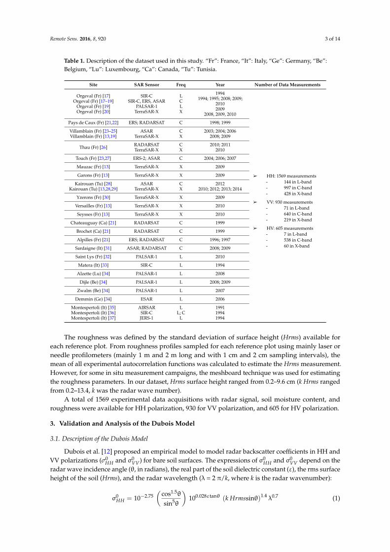
Table 1. Description of the dataset used in this study. “Fr”: France, “It”: Italy, “Ge”: Germany, “Be”:Belgium, “Lu”: Luxembourg, “Ca”: Canada, “Tu”: Tunisia.
Site SAR Sensor Freq Year Number of Data Measurements
Orgeval (Fr) [17]Orgeval (Fr) [17–19]
Orgeval (Fr) [19]Orgeval (Fr) [20]
SIR-CSIR-C, ERS, ASAR
PALSAR-1TerraSAR-X
LCLX
19941994; 1995; 2008; 2009;
20102009
2008, 2009, 2010
â HH: 1569 measurements- 144 in L-band- 997 in C-band- 428 in X-band
â VV: 930 measurements- 71 in L-band- 640 in C-band- 219 in X-band
â HV: 605 measurements- 7 in L-band- 538 in C-band- 60 in X-band
Pays de Caux (Fr) [21,22] ERS; RADARSAT C 1998; 1999
Villamblain (Fr) [23–25]Villamblain (Fr) [13,19]
ASARTerraSAR-X
CX
2003; 2004; 20062008; 2009
Thau (Fr) [26] RADARSATTerraSAR-X
CX
2010; 20112010
Touch (Fr) [23,27] ERS-2; ASAR C 2004; 2006; 2007
Mauzac (Fr) [13] TerraSAR-X X 2009
Garons (Fr) [13] TerraSAR-X X 2009
Kairouan (Tu) [28]Kairouan (Tu) [13,28,29]
ASARTerraSAR-X
CX
20122010; 2012; 2013; 2014
Yzerons (Fr) [30] TerraSAR-X X 2009
Versailles (Fr) [13] TerraSAR-X X 2010
Seysses (Fr) [13] TerraSAR-X X 2010
Chateauguay (Ca) [21] RADARSAT C 1999
Brochet (Ca) [21] RADARSAT C 1999
Alpilles (Fr) [21] ERS; RADARSAT C 1996; 1997
Sardaigne (It) [31] ASAR; RADARSAT C 2008; 2009
Saint Lys (Fr) [32] PALSAR-1 L 2010
Matera (It) [33] SIR-C L 1994
Alzette (Lu) [34] PALSAR-1 L 2008
Dijle (Be) [34] PALSAR-1 L 2008; 2009
Zwalm (Be) [34] PALSAR-1 L 2007
Demmin (Ge) [34] ESAR L 2006
Montespertoli (It) [35]Montespertoli (It) [36]Montespertoli (It) [37]
AIRSARSIR-CJERS-1
LL; C
L
199119941994
The roughness was defined by the standard deviation of surface height (Hrms) available foreach reference plot. From roughness profiles sampled for each reference plot using mainly laser orneedle profilometers (mainly 1 m and 2 m long and with 1 cm and 2 cm sampling intervals), themean of all experimental autocorrelation functions was calculated to estimate the Hrms measurement.However, for some in situ measurement campaigns, the meshboard technique was used for estimatingthe roughness parameters. In our dataset, Hrms surface height ranged from 0.2–9.6 cm (k Hrms rangedfrom 0.2–13.4, k was the radar wave number).
A total of 1569 experimental data acquisitions with radar signal, soil moisture content, androughness were available for HH polarization, 930 for VV polarization, and 605 for HV polarization.
3. Validation and Analysis of the Dubois Model
3.1. Description of the Dubois Model
Dubois et al. [12] proposed an empirical model to model radar backscatter coefficients in HH andVV polarizations (σ0
HH and σ0VV) for bare soil surfaces. The expressions of σ0
HH and σ0VV depend on the
radar wave incidence angle (θ, in radians), the real part of the soil dielectric constant (ε), the rms surfaceheight of the soil (Hrms), and the radar wavelength (λ = 2 π/k, where k is the radar wavenumber):
σ0HH = 10−2.75
(cos1.5θ
sin5θ
)100.028εtanθ (k Hrmssinθ)1.4 λ0.7 (1)
Remote Sens. 2016, 8, 920 4 of 14
σ0VV = 10−2.35
(cos3θ
sin3θ
)100.046εtanθ (k Hrmssinθ)1.1 λ0.7 (2)
σ0HH and σ0
VV are given in a linear scale. λ is in cm. The validity of the Dubois model is defined asfollows: k Hrms ≤ 2.5, mv ≤ 35 vol%, and θ ≥ 30◦.
3.2. Comparison between Simulated and Real Data
The Dubois model shows an overestimation of the radar signal by 0.7 dB in HH polarization andan underestimation of the radar signal by 0.9 dB in VV polarization for all data combined (Table 2).The results show that the overestimation in HH is of the same order for L-, C-, and X-bands (between0.6–0.8 dB). For the L-band, a slight overestimation of approximately 0.2 dB of SAR data is observed inVV polarization. Additionally, in VV polarization, the Dubois model-based simulations underestimatethe SAR data in the C- and X-bands by approximately 0.7 dB and 2.0 dB, respectively.
The rms error (RMSE) is approximately 3.8 dB and 2.8 dB in HH and VV, respectively (Table 2).Analysis of the RMSE according the radar frequency band (L-, C-, and X-, separately) shows in HH anincrease of the RMSE with the radar frequency (2.9 dB in the L-band, 3.7 dB in the C-band, and 4.1 dBin the X-band). In VV polarization, the quality of Dubois simulations (RMSE) is similar for the L- andC-bands, but is less accurate in the X-band (2.3 dB in the L-band, 2.6 dB in the C-band, and 3.2 dB inthe X-band).
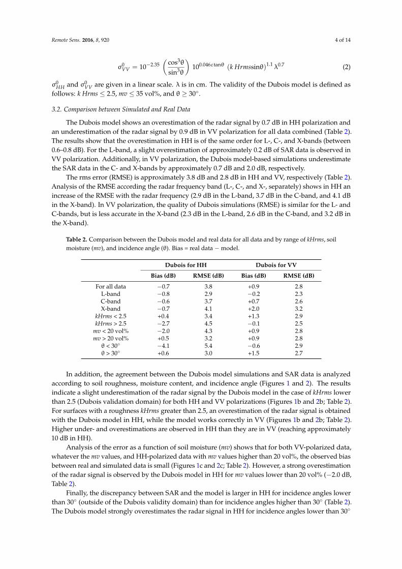
Table 2. Comparison between the Dubois model and real data for all data and by range of kHrms, soilmoisture (mv), and incidence angle (θ). Bias = real data − model.
Dubois for HH Dubois for VV
Bias (dB) RMSE (dB) Bias (dB) RMSE (dB)
For all data −0.7 3.8 +0.9 2.8L-band −0.8 2.9 −0.2 2.3C-band −0.6 3.7 +0.7 2.6X-band −0.7 4.1 +2.0 3.2
kHrms < 2.5 +0.4 3.4 +1.3 2.9kHrms > 2.5 −2.7 4.5 −0.1 2.5
mv < 20 vol% −2.0 4.3 +0.9 2.8mv > 20 vol% +0.5 3.2 +0.9 2.8θ < 30◦ −4.1 5.4 −0.6 2.9θ > 30◦ +0.6 3.0 +1.5 2.7
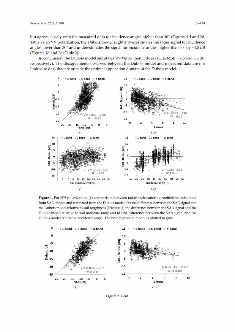
In addition, the agreement between the Dubois model simulations and SAR data is analyzedaccording to soil roughness, moisture content, and incidence angle (Figures 1 and 2). The resultsindicate a slight underestimation of the radar signal by the Dubois model in the case of kHrms lowerthan 2.5 (Dubois validation domain) for both HH and VV polarizations (Figures 1b and 2b; Table 2).For surfaces with a roughness kHrms greater than 2.5, an overestimation of the radar signal is obtainedwith the Dubois model in HH, while the model works correctly in VV (Figures 1b and 2b; Table 2).Higher under- and overestimations are observed in HH than they are in VV (reaching approximately10 dB in HH).
Analysis of the error as a function of soil moisture (mv) shows that for both VV-polarized data,whatever the mv values, and HH-polarized data with mv values higher than 20 vol%, the observed biasbetween real and simulated data is small (Figures 1c and 2c; Table 2). However, a strong overestimationof the radar signal is observed by the Dubois model in HH for mv values lower than 20 vol% (−2.0 dB,Table 2).
Finally, the discrepancy between SAR and the model is larger in HH for incidence angles lowerthan 30◦ (outside of the Dubois validity domain) than for incidence angles higher than 30◦ (Table 2).The Dubois model strongly overestimates the radar signal in HH for incidence angles lower than 30◦
Remote Sens. 2016, 8, 920 5 of 14
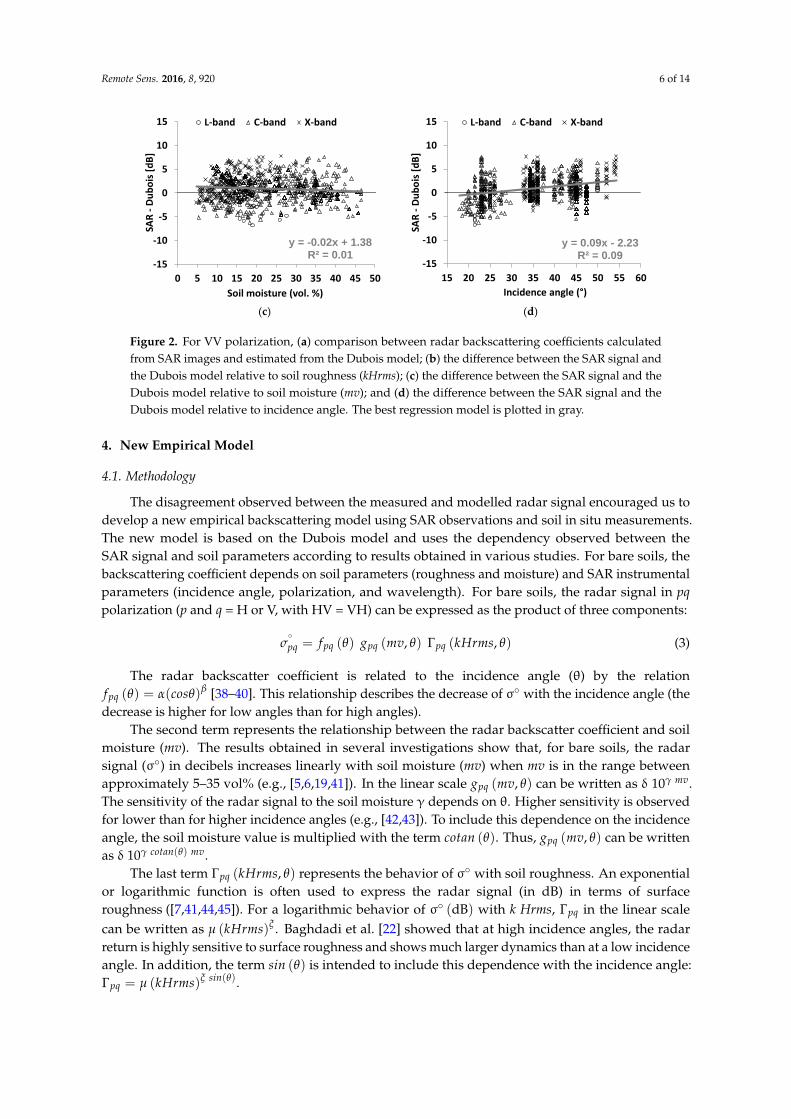
but agrees closely with the measured data for incidence angles higher than 30◦ (Figures 1d and 2d;Table 2). In VV polarization, the Dubois model slightly overestimates the radar signal for incidenceangles lower than 30◦ and underestimates the signal for incidence angles higher than 30◦ by +1.5 dB(Figures 1d and 2d; Table 2).
In conclusion, the Dubois model simulates VV better than it does HH (RMSE = 2.8 and 3.8 dB,respectively). The disagreements observed between the Dubois model and measured data are notlimited to data that are outside the optimal application domain of the Dubois model.
Remote Sens. 2016, 8, 920 5 of 14
The Dubois model strongly overestimates the radar signal in HH for incidence angles lower than 30°
but agrees closely with the measured data for incidence angles higher than 30° (Figures 1d and 2d;
Table 2). In VV polarization, the Dubois model slightly overestimates the radar signal for incidence
angles lower than 30° and underestimates the signal for incidence angles higher than 30° by +1.5 dB
(Figures 1d and 2d; Table 2).
In conclusion, the Dubois model simulates VV better than it does HH (RMSE = 2.8 and 3.8 dB,
respectively). The disagreements observed between the Dubois model and measured data are not
limited to data that are outside the optimal application domain of the Dubois model.
(a) (b)
(c) (d)
Figure 1. For HH polarization, (a) comparison between radar backscattering coefficients calculated
from SAR images and estimated from the Dubois model; (b) the difference between the SAR signal
and the Dubois model relative to soil roughness (kHrms); (c) the difference between the SAR signal
and the Dubois model relative to soil moisture (mv); and (d) the difference between the SAR signal
and the Dubois model relative to incidence angle. The best regression model is plotted in gray.
(a) (b)
y = 0.94x + 0.06R² = 0.37
-25
-20
-15
-10
-5
0
5
-25 -20 -15 -10 -5 0 5
Du
bo
is [
dB
]
SAR [dB]
L-band C-band X-band
y = -1.02x + 1.81R² = 0.20
-15
-10
-5
0
5
10
15
0 2 4 6 8 10SA
R -
Du
bo
is [
dB
]
k Hrms
L-band C-band X-band
y = 0.12x - 3.40R² = 0.13
-15
-10
-5
0
5
10
15
0 5 10 15 20 25 30 35 40 45 50
SAR
-D
ub
ois
[d
B]
Soil moisture (vol. %)
L-band C-band X-band
y = 0.23x - 9.28R² = 0.31
-15
-10
-5
0
5
10
15
15 20 25 30 35 40 45 50 55 60
SAR
-D
ub
ois
[d
B]
Incidence angle (°)
L-band C-band X-band
y = 0.87x - 2.07R² = 0.49
-25
-20
-15
-10
-5
0
5
-25 -20 -15 -10 -5 0 5
Du
bo
is [
dB
]
SAR [dB]
L-band C-band X-band
y = -0.61x + 2.23R² = 0.09
-15
-10
-5
0
5
10
15
0 2 4 6 8 10
SAR
-D
ub
ois
[d
B]
k Hrms
L-band C-band X-band
Figure 1. For HH polarization, (a) comparison between radar backscattering coefficients calculatedfrom SAR images and estimated from the Dubois model; (b) the difference between the SAR signal andthe Dubois model relative to soil roughness (kHrms); (c) the difference between the SAR signal and theDubois model relative to soil moisture (mv); and (d) the difference between the SAR signal and theDubois model relative to incidence angle. The best regression model is plotted in gray.
Remote Sens. 2016, 8, 920 5 of 14
The Dubois model strongly overestimates the radar signal in HH for incidence angles lower than 30°
but agrees closely with the measured data for incidence angles higher than 30° (Figures 1d and 2d;
Table 2). In VV polarization, the Dubois model slightly overestimates the radar signal for incidence
angles lower than 30° and underestimates the signal for incidence angles higher than 30° by +1.5 dB
(Figures 1d and 2d; Table 2).
In conclusion, the Dubois model simulates VV better than it does HH (RMSE = 2.8 and 3.8 dB,
respectively). The disagreements observed between the Dubois model and measured data are not
limited to data that are outside the optimal application domain of the Dubois model.
(a) (b)
(c) (d)
Figure 1. For HH polarization, (a) comparison between radar backscattering coefficients calculated
from SAR images and estimated from the Dubois model; (b) the difference between the SAR signal
and the Dubois model relative to soil roughness (kHrms); (c) the difference between the SAR signal
and the Dubois model relative to soil moisture (mv); and (d) the difference between the SAR signal
and the Dubois model relative to incidence angle. The best regression model is plotted in gray.
(a) (b)
y = 0.94x + 0.06R² = 0.37
-25
-20
-15
-10
-5
0
5
-25 -20 -15 -10 -5 0 5
Du
bo
is [
dB
]
SAR [dB]
L-band C-band X-band
y = -1.02x + 1.81R² = 0.20
-15
-10
-5
0
5
10
15
0 2 4 6 8 10
SAR
-D
ub
ois
[d
B]
k Hrms
L-band C-band X-band
y = 0.12x - 3.40R² = 0.13
-15
-10
-5
0
5
10
15
0 5 10 15 20 25 30 35 40 45 50
SAR
-D
ub
ois
[d
B]
Soil moisture (vol. %)
L-band C-band X-band
y = 0.23x - 9.28R² = 0.31
-15
-10
-5
0
5
10
15
15 20 25 30 35 40 45 50 55 60
SAR
-D
ub
ois
[d
B]
Incidence angle (°)
L-band C-band X-band
y = 0.87x - 2.07R² = 0.49
-25
-20
-15
-10
-5
0
5
-25 -20 -15 -10 -5 0 5
Du
bo
is [
dB
]
SAR [dB]
L-band C-band X-band
y = -0.61x + 2.23R² = 0.09
-15
-10
-5
0
5
10
15
0 2 4 6 8 10
SAR
-D
ub
ois
[d
B]
k Hrms
L-band C-band X-band
Figure 2. Cont.
Remote Sens. 2016, 8, 920 6 of 14Remote Sens. 2016, 8, 920 6 of 14
(c) (d)
Figure 2. For VV polarization, (a) comparison between radar backscattering coefficients calculated
from SAR images and estimated from the Dubois model; (b) the difference between the SAR signal
and the Dubois model relative to soil roughness (kHrms); (c) the difference between the SAR signal
and the Dubois model relative to soil moisture (mv); and (d) the difference between the SAR signal
and the Dubois model relative to incidence angle. The best regression model is plotted in gray.
4. New Empirical Model
4.1. Methodology
The disagreement observed between the measured and modelled radar signal encouraged us to
develop a new empirical backscattering model using SAR observations and soil in situ
measurements. The new model is based on the Dubois model and uses the dependency observed
between the SAR signal and soil parameters according to results obtained in various studies. For bare
soils, the backscattering coefficient depends on soil parameters (roughness and moisture) and SAR
instrumental parameters (incidence angle, polarization, and wavelength). For bare soils, the radar
signal in pq polarization (p and q = H or V, with HV = VH) can be expressed as the product of three
components:
𝜎𝑝𝑞° = 𝑓𝑝𝑞(𝜃) 𝑔𝑝𝑞(𝑚𝑣, 𝜃) Γ𝑝𝑞(𝑘𝐻𝑟𝑚𝑠, 𝜃) (3)
The radar backscatter coefficient is related to the incidence angle () by the relation
𝑓𝑝𝑞(𝜃) = 𝛼(𝑐𝑜𝑠 𝜃)𝛽 [38–40]. This relationship describes the decrease of ° with the incidence angle
(the decrease is higher for low angles than for high angles).
The second term represents the relationship between the radar backscatter coefficient and soil
moisture (mv). The results obtained in several investigations show that, for bare soils, the radar signal
(°) in decibels increases linearly with soil moisture (mv) when mv is in the range between
approximately 5–35 vol% (e.g., [5,6,19,41]). In the linear scale 𝑔𝑝𝑞(𝑚𝑣, 𝜃) can be written as
δ 10𝛾 𝑚𝑣 . The sensitivity of the radar signal to the soil moisture depends on . Higher sensitivity is
observed for lower than for higher incidence angles (e.g., [42,43]). To include this dependence on the
incidence angle, the soil moisture value is multiplied with the term 𝑐𝑜𝑡𝑎𝑛(𝜃). Thus, 𝑔𝑝𝑞(𝑚𝑣, 𝜃) can
be written as δ 10𝛾 𝑐𝑜𝑡𝑎𝑛(𝜃) 𝑚𝑣.
The last term Γ𝑝𝑞(𝑘𝐻𝑟𝑚𝑠, 𝜃) represents the behavior of ° with soil roughness. An exponential or
logarithmic function is often used to express the radar signal (in dB) in terms of surface roughness
([7,41,44,45]). For a logarithmic behavior of °(dB) with k Hrms, Γ𝑝𝑞 in the linear scale can be written
as 𝜇(𝑘𝐻𝑟𝑚𝑠)𝜉. Baghdadi et al. [22] showed that at high incidence angles, the radar return is highly
sensitive to surface roughness and shows much larger dynamics than at a low incidence angle. In
addition, the term 𝑠𝑖𝑛(𝜃) is intended to include this dependence with the incidence angle:
Γ𝑝𝑞=𝜇(𝑘𝐻𝑟𝑚𝑠)𝜉 𝑠𝑖𝑛 (𝜃).
Finally, the relationship between the radar backscattering coefficient (°) and the soil parameters
(soil moisture and surface roughness) for bare soil surfaces can be written as Equation (4):
y = -0.02x + 1.38R² = 0.01
-15
-10
-5
0
5
10
15
0 5 10 15 20 25 30 35 40 45 50
SAR
-D
ub
ois
[d
B]
Soil moisture (vol. %)
L-band C-band X-band
y = 0.09x - 2.23R² = 0.09
-15
-10
-5
0
5
10
15
15 20 25 30 35 40 45 50 55 60
SAR
-D
ub
ois
[d
B]
Incidence angle (°)
L-band C-band X-band
Figure 2. For VV polarization, (a) comparison between radar backscattering coefficients calculatedfrom SAR images and estimated from the Dubois model; (b) the difference between the SAR signal andthe Dubois model relative to soil roughness (kHrms); (c) the difference between the SAR signal and theDubois model relative to soil moisture (mv); and (d) the difference between the SAR signal and theDubois model relative to incidence angle. The best regression model is plotted in gray.
4. New Empirical Model
4.1. Methodology
The disagreement observed between the measured and modelled radar signal encouraged us todevelop a new empirical backscattering model using SAR observations and soil in situ measurements.The new model is based on the Dubois model and uses the dependency observed between theSAR signal and soil parameters according to results obtained in various studies. For bare soils, thebackscattering coefficient depends on soil parameters (roughness and moisture) and SAR instrumentalparameters (incidence angle, polarization, and wavelength). For bare soils, the radar signal in pqpolarization (p and q = H or V, with HV = VH) can be expressed as the product of three components:
σ◦pq = fpq (θ) gpq (mv, θ) Γpq (kHrms, θ) (3)
The radar backscatter coefficient is related to the incidence angle (θ) by the relationfpq (θ) = α(cosθ)β [38–40]. This relationship describes the decrease of σ◦ with the incidence angle (thedecrease is higher for low angles than for high angles).
The second term represents the relationship between the radar backscatter coefficient and soilmoisture (mv). The results obtained in several investigations show that, for bare soils, the radarsignal (σ◦) in decibels increases linearly with soil moisture (mv) when mv is in the range betweenapproximately 5–35 vol% (e.g., [5,6,19,41]). In the linear scale gpq (mv, θ) can be written as δ 10γ mv.The sensitivity of the radar signal to the soil moisture γ depends on θ. Higher sensitivity is observedfor lower than for higher incidence angles (e.g., [42,43]). To include this dependence on the incidenceangle, the soil moisture value is multiplied with the term cotan (θ). Thus, gpq (mv, θ) can be writtenas δ 10γ cotan(θ) mv.
The last term Γpq (kHrms, θ) represents the behavior of σ◦ with soil roughness. An exponentialor logarithmic function is often used to express the radar signal (in dB) in terms of surfaceroughness ([7,41,44,45]). For a logarithmic behavior of σ◦ (dB) with k Hrms, Γpq in the linear scalecan be written as µ (kHrms)ξ . Baghdadi et al. [22] showed that at high incidence angles, the radarreturn is highly sensitive to surface roughness and shows much larger dynamics than at a low incidenceangle. In addition, the term sin (θ) is intended to include this dependence with the incidence angle:Γpq = µ (kHrms)ξ sin(θ).
Remote Sens. 2016, 8, 920 7 of 14
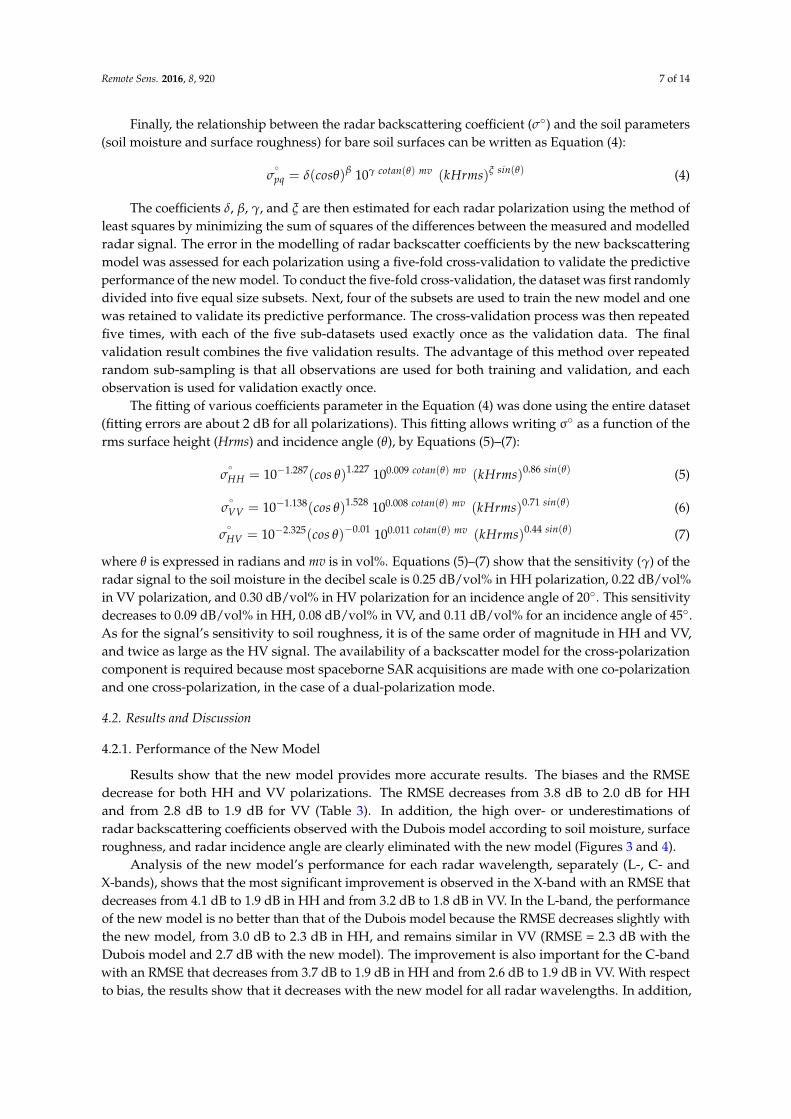
Finally, the relationship between the radar backscattering coefficient (σ◦) and the soil parameters(soil moisture and surface roughness) for bare soil surfaces can be written as Equation (4):
σ◦pq = δ(cosθ)β 10γ cotan(θ) mv (kHrms)ξ sin(θ) (4)
The coefficients δ, β, γ, and ξ are then estimated for each radar polarization using the method ofleast squares by minimizing the sum of squares of the differences between the measured and modelledradar signal. The error in the modelling of radar backscatter coefficients by the new backscatteringmodel was assessed for each polarization using a five-fold cross-validation to validate the predictiveperformance of the new model. To conduct the five-fold cross-validation, the dataset was first randomlydivided into five equal size subsets. Next, four of the subsets are used to train the new model and onewas retained to validate its predictive performance. The cross-validation process was then repeatedfive times, with each of the five sub-datasets used exactly once as the validation data. The finalvalidation result combines the five validation results. The advantage of this method over repeatedrandom sub-sampling is that all observations are used for both training and validation, and eachobservation is used for validation exactly once.
The fitting of various coefficients parameter in the Equation (4) was done using the entire dataset(fitting errors are about 2 dB for all polarizations). This fitting allows writing σ◦ as a function of therms surface height (Hrms) and incidence angle (θ), by Equations (5)–(7):
σ◦HH = 10−1.287(cos θ)1.227 100.009 cotan(θ) mv (kHrms)0.86 sin(θ) (5)
σ◦VV = 10−1.138(cos θ)1.528 100.008 cotan(θ) mv (kHrms)0.71 sin(θ) (6)
σ◦HV = 10−2.325(cos θ)−0.01 100.011 cotan(θ) mv (kHrms)0.44 sin(θ) (7)
where θ is expressed in radians and mv is in vol%. Equations (5)–(7) show that the sensitivity (γ) of theradar signal to the soil moisture in the decibel scale is 0.25 dB/vol% in HH polarization, 0.22 dB/vol%in VV polarization, and 0.30 dB/vol% in HV polarization for an incidence angle of 20◦. This sensitivitydecreases to 0.09 dB/vol% in HH, 0.08 dB/vol% in VV, and 0.11 dB/vol% for an incidence angle of 45◦.As for the signal’s sensitivity to soil roughness, it is of the same order of magnitude in HH and VV,and twice as large as the HV signal. The availability of a backscatter model for the cross-polarizationcomponent is required because most spaceborne SAR acquisitions are made with one co-polarizationand one cross-polarization, in the case of a dual-polarization mode.
4.2. Results and Discussion
4.2.1. Performance of the New Model
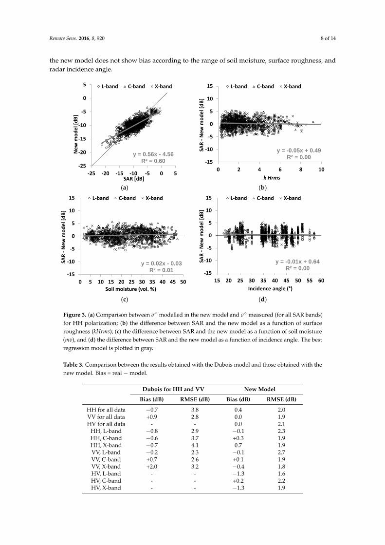
Results show that the new model provides more accurate results. The biases and the RMSEdecrease for both HH and VV polarizations. The RMSE decreases from 3.8 dB to 2.0 dB for HHand from 2.8 dB to 1.9 dB for VV (Table 3). In addition, the high over- or underestimations ofradar backscattering coefficients observed with the Dubois model according to soil moisture, surfaceroughness, and radar incidence angle are clearly eliminated with the new model (Figures 3 and 4).
Analysis of the new model’s performance for each radar wavelength, separately (L-, C- andX-bands), shows that the most significant improvement is observed in the X-band with an RMSE thatdecreases from 4.1 dB to 1.9 dB in HH and from 3.2 dB to 1.8 dB in VV. In the L-band, the performanceof the new model is no better than that of the Dubois model because the RMSE decreases slightly withthe new model, from 3.0 dB to 2.3 dB in HH, and remains similar in VV (RMSE = 2.3 dB with theDubois model and 2.7 dB with the new model). The improvement is also important for the C-bandwith an RMSE that decreases from 3.7 dB to 1.9 dB in HH and from 2.6 dB to 1.9 dB in VV. With respectto bias, the results show that it decreases with the new model for all radar wavelengths. In addition,
Remote Sens. 2016, 8, 920 8 of 14
the new model does not show bias according to the range of soil moisture, surface roughness, andradar incidence angle.Remote Sens. 2016, 8, 920 8 of 14
(a) (b)
(c) (d)
Figure 3. (a) Comparison between ° modelled in the new model and ° measured (for all SAR bands)
for HH polarization; (b) the difference between SAR and the new model as a function of surface
roughness (kHrms); (c) the difference between SAR and the new model as a function of soil moisture
(mv), and (d) the difference between SAR and the new model as a function of incidence angle. The
best regression model is plotted in gray.
Table 3. Comparison between the results obtained with the Dubois model and those obtained with
the new model. Bias = real − model.
Dubois for HH and VV New Model
Bias (dB) RMSE (dB) Bias (dB) RMSE (dB)
HH for all data −0.7 3.8 0.4 2.0
VV for all data +0.9 2.8 0.0 1.9
HV for all data - - 0.0 2.1
HH, L-band −0.8 2.9 −0.1 2.3
HH, C-band −0.6 3.7 +0.3 1.9
HH, X-band −0.7 4.1 0.7 1.9
VV, L-band −0.2 2.3 −0.1 2.7
VV, C-band +0.7 2.6 +0.1 1.9
VV, X-band +2.0 3.2 −0.4 1.8
HV, L-band - - −1.3 1.6
HV, C-band - - +0.2 2.2
HV, X-band - - −1.3 1.9
y = 0.56x - 4.56R² = 0.60
-25
-20
-15
-10
-5
0
5
-25 -20 -15 -10 -5 0 5
New
mo
de
l [d
B]
SAR [dB]
L-band C-band X-band
y = -0.05x + 0.49R² = 0.00
-15
-10
-5
0
5
10
15
0 2 4 6 8 10
SAR
-N
ew m
od
el [
dB
]
k Hrms
L-band C-band X-band
y = 0.02x - 0.03R² = 0.01
-15
-10
-5
0
5
10
15
0 5 10 15 20 25 30 35 40 45 50
SAR
-N
ew m
od
el [
dB
]
Soil moisture (vol. %)
L-band C-band X-band
y = -0.01x + 0.64R² = 0.00
-15
-10
-5
0
5
10
15
15 20 25 30 35 40 45 50 55 60
SAR
-N
ew m
od
el [
dB
]
Incidence angle (°)
L-band C-band X-band
Figure 3. (a) Comparison between σ◦ modelled in the new model and σ◦ measured (for all SAR bands)for HH polarization; (b) the difference between SAR and the new model as a function of surfaceroughness (kHrms); (c) the difference between SAR and the new model as a function of soil moisture(mv), and (d) the difference between SAR and the new model as a function of incidence angle. The bestregression model is plotted in gray.
Table 3. Comparison between the results obtained with the Dubois model and those obtained with thenew model. Bias = real − model.
Dubois for HH and VV New Model
Bias (dB) RMSE (dB) Bias (dB) RMSE (dB)
HH for all data −0.7 3.8 0.4 2.0VV for all data +0.9 2.8 0.0 1.9HV for all data - - 0.0 2.1
HH, L-band −0.8 2.9 −0.1 2.3HH, C-band −0.6 3.7 +0.3 1.9HH, X-band −0.7 4.1 0.7 1.9VV, L-band −0.2 2.3 −0.1 2.7VV, C-band +0.7 2.6 +0.1 1.9VV, X-band +2.0 3.2 −0.4 1.8HV, L-band - - −1.3 1.6HV, C-band - - +0.2 2.2HV, X-band - - −1.3 1.9
Remote Sens. 2016, 8, 920 9 of 14Remote Sens. 2016, 8, 920 9 of 14
(a) (b)
(c) (d)
Figure 4. (a) Comparison between ° in the new model and ° measured (for all SAR bands) for VV
polarization; (b) the difference between SAR and the new model as a function of surface roughness
(kHrms); (c) the difference between SAR and the new model as a function of soil moisture (mv); and
(d) the difference between SAR and the new model as a function of incidence angle. The best
regression model is plotted in gray.
The comparison between the new model simulations in HV polarization Equation (7) and the
real data (SAR data) shows an RMSE of 2.1 dB (Table 3) (1.6 dB in the L-band, 2.2 dB in the C-band,
and 1.9 dB in the X-band). The bias (°SAR—model) is −1.3 dB in the L-band, 0.2 dB in the C-band,
and −1.3 dB in the X-band. Figure 5 shows also that the new model correctly simulates the radar
backscatter coefficient in HV for all ranges of soil moisture, surface roughness, and radar incidence angle.
(a) (b)
y = 0.57x - 3.90R² = 0.57
-25
-20
-15
-10
-5
0
5
-25 -20 -15 -10 -5 0 5
New
mo
de
l [d
B]
SAR [dB]
L-band C-band X-band
y = -0.14x + 0.30R² = 0.01
-15
-10
-5
0
5
10
15
0 2 4 6 8 10
SAR
-N
ew m
od
el [
dB
]
k Hrms
L-band C-band X-band
y = 0.02x - 0.52R² = 0.02
-15
-10
-5
0
5
10
15
0 5 10 15 20 25 30 35 40 45 50
SAR
-N
ew m
od
el [
dB
]
Soil moisture (vol. %)
L-band C-band X-band
y = 0.00x - 0.07R² = 0.00
-15
-10
-5
0
5
10
15
15 20 25 30 35 40 45 50 55 60
SAR
-N
ew m
od
el [
dB
]
Incidence angle (°)
L-band C-band X-band
y = 0.41x - 11.32R² = 0.41
-35
-30
-25
-20
-15
-10
-5
-35 -30 -25 -20 -15 -10 -5
New
mo
de
l [d
B]
SAR [dB]
L-band C-band X-band
y = -0.14x + 0.29R² = 0.01
-15
-10
-5
0
5
10
15
0 2 4 6 8 10
SAR
-N
ew m
od
el [
dB
]
k Hrms
L-band C-band X-band
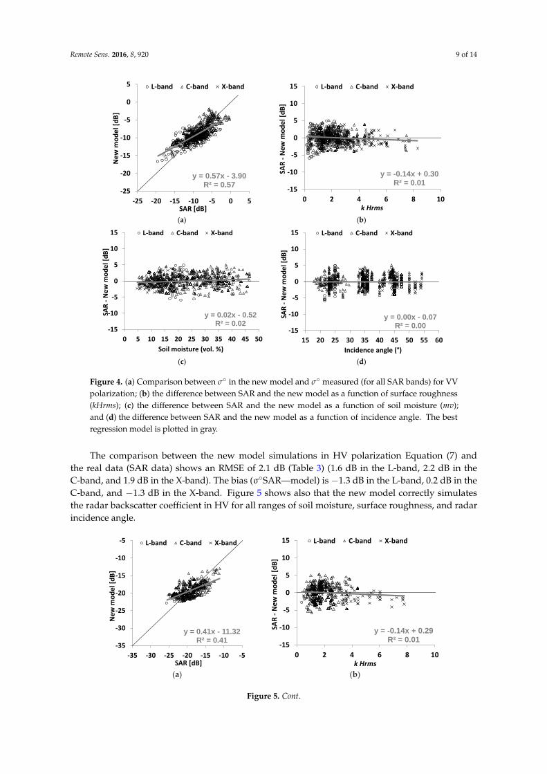
Figure 4. (a) Comparison between σ◦ in the new model and σ◦ measured (for all SAR bands) for VVpolarization; (b) the difference between SAR and the new model as a function of surface roughness(kHrms); (c) the difference between SAR and the new model as a function of soil moisture (mv);and (d) the difference between SAR and the new model as a function of incidence angle. The bestregression model is plotted in gray.
The comparison between the new model simulations in HV polarization Equation (7) andthe real data (SAR data) shows an RMSE of 2.1 dB (Table 3) (1.6 dB in the L-band, 2.2 dB in theC-band, and 1.9 dB in the X-band). The bias (σ◦SAR—model) is −1.3 dB in the L-band, 0.2 dB in theC-band, and −1.3 dB in the X-band. Figure 5 shows also that the new model correctly simulatesthe radar backscatter coefficient in HV for all ranges of soil moisture, surface roughness, and radarincidence angle.
Remote Sens. 2016, 8, 920 9 of 14
(a) (b)
(c) (d)
Figure 4. (a) Comparison between ° in the new model and ° measured (for all SAR bands) for VV
polarization; (b) the difference between SAR and the new model as a function of surface roughness
(kHrms); (c) the difference between SAR and the new model as a function of soil moisture (mv); and
(d) the difference between SAR and the new model as a function of incidence angle. The best
regression model is plotted in gray.
The comparison between the new model simulations in HV polarization Equation (7) and the
real data (SAR data) shows an RMSE of 2.1 dB (Table 3) (1.6 dB in the L-band, 2.2 dB in the C-band,
and 1.9 dB in the X-band). The bias (°SAR—model) is −1.3 dB in the L-band, 0.2 dB in the C-band,
and −1.3 dB in the X-band. Figure 5 shows also that the new model correctly simulates the radar
backscatter coefficient in HV for all ranges of soil moisture, surface roughness, and radar incidence angle.
(a) (b)
y = 0.57x - 3.90R² = 0.57
-25
-20
-15
-10
-5
0
5
-25 -20 -15 -10 -5 0 5
New
mo
de
l [d
B]
SAR [dB]
L-band C-band X-band
y = -0.14x + 0.30R² = 0.01
-15
-10
-5
0
5
10
15
0 2 4 6 8 10
SAR
-N
ew m
od
el [
dB
]
k Hrms
L-band C-band X-band
y = 0.02x - 0.52R² = 0.02
-15
-10
-5
0
5
10
15
0 5 10 15 20 25 30 35 40 45 50
SAR
-N
ew m
od
el [
dB
]
Soil moisture (vol. %)
L-band C-band X-band
y = 0.00x - 0.07R² = 0.00
-15
-10
-5
0
5
10
15
15 20 25 30 35 40 45 50 55 60
SAR
-N
ew m
od
el [
dB
]
Incidence angle (°)
L-band C-band X-band
y = 0.41x - 11.32R² = 0.41
-35
-30
-25
-20
-15
-10
-5
-35 -30 -25 -20 -15 -10 -5
New
mo
de
l [d
B]
SAR [dB]
L-band C-band X-band
y = -0.14x + 0.29R² = 0.01
-15
-10
-5
0
5
10
15
0 2 4 6 8 10
SAR
-N
ew m
od
el [
dB
]
k Hrms
L-band C-band X-band
Figure 5. Cont.
Remote Sens. 2016, 8, 920 10 of 14Remote Sens. 2016, 8, 920 10 of 14
(c) (d)
Figure 5. (a) Comparison between ° in the new model and ° measured (for all SAR bands) for HV
polarization; (b) the difference between SAR and the new model as a function of kHrms; (c) the
difference between SAR and the new model as a function of mv; and (d) the difference between SAR
and the new model as a function of incidence angle. The best regression model is plotted in gray.
4.2.2. Behavior of the New Model
The physical behavior of the new radar backscatter model was studied as a function of the
incidence angle (), soil moisture (mv), and surface roughness (kHrms).
Figure 6 shows that the radar signal is strongly sensitive to surface roughness, especially for
small values of kHrms. In addition, this sensitivity increases with the incidence angle. Concerning the
influence of polarization, the new model shows, as do many theories and experimental studies, that
a given soil roughness leads to slightly higher signal dynamics with the soil moisture in HH than in
VV polarization [17,46]. The radar signal ° increases with kHrms. This increase is higher for either
low kHrms values or high values than it is for either high kHrms values or low values. For = 45°,
° increases approximately 8 dB in HH and 6.5 dB in VV when kHrms increases from 0.1 to 2
compared with only 3 dB when kHrms increases from two to six (for both HH and VV). This dynamic
of ° is only half for = 25° in comparison to that for = 45°. In HV, the dynamic of ° to kHrms is
half that observed for HH and VV.
The behavior of ° according to soil moisture shows a larger increase of ° with mv for low incidence
angles than for high incidence angles. Figure 6 shows that °HH and °VV increase approximately 6 dB for
= 25° compared with only 3 dB for = 45° when mv increases from five to 35 vol%. In HV, the signal
increases approximately 7.5 dB for = 25° and 3.5 dB for = 45° when mv increases from 5 to 35 vol%.
As mentioned in Dubois et al. [12], the ratio 𝜎𝐻𝐻°
𝜎𝑉𝑉°⁄ should increase with kHrms and remain less
than 1. The new model shows that this condition is satisfied when 20°< < 45°, kHrms < 6 and mv < 35 vol%.
(a) (b)
y = 0.01x - 0.28R² = 0.00
-15
-10
-5
0
5
10
15
0 5 10 15 20 25 30 35 40 45 50
SAR
-N
ew m
od
el [
dB
]
Soil moisture (vol. %)
L-band C-band X-band
y = 0.01x - 0.24R² = 0.00
-15
-10
-5
0
5
10
15
15 20 25 30 35 40 45 50 55 60
SAR
-N
ew m
od
el [
dB
]
Incidence angle (°)
L-band C-band X-band
-25
-20
-15
-10
-5
0
0 1 2 3 4 5 6
HH
[d
B]
k Hrms
Incidence angle = 25°
mv=5 vol.%
mv=15 vol.%
mv=35 vol.%-25
-20
-15
-10
-5
0
0 1 2 3 4 5 6
HH
[d
B]
k Hrms
Incidence angle = 45°
mv=5 vol.%
mv=15 vol.%
mv=35 vol.%
Figure 5. (a) Comparison between σ◦ in the new model and σ◦ measured (for all SAR bands) forHV polarization; (b) the difference between SAR and the new model as a function of kHrms; (c) thedifference between SAR and the new model as a function of mv; and (d) the difference between SARand the new model as a function of incidence angle. The best regression model is plotted in gray.
4.2.2. Behavior of the New Model
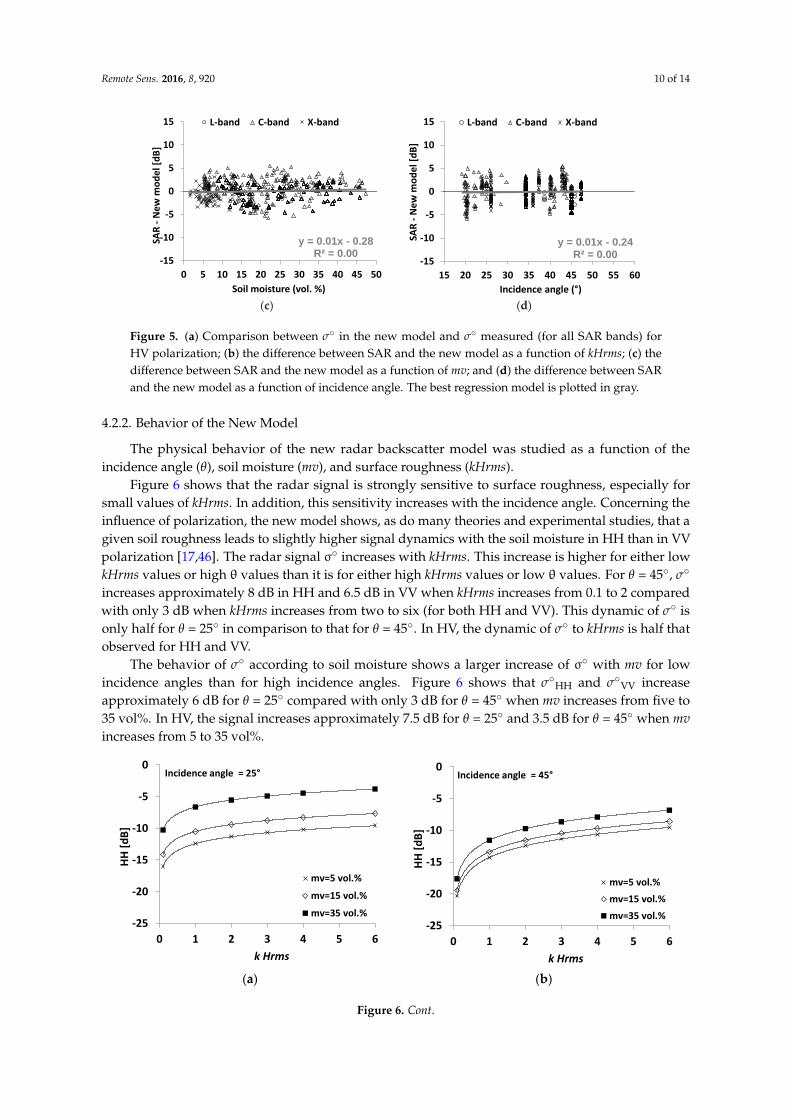
The physical behavior of the new radar backscatter model was studied as a function of theincidence angle (θ), soil moisture (mv), and surface roughness (kHrms).
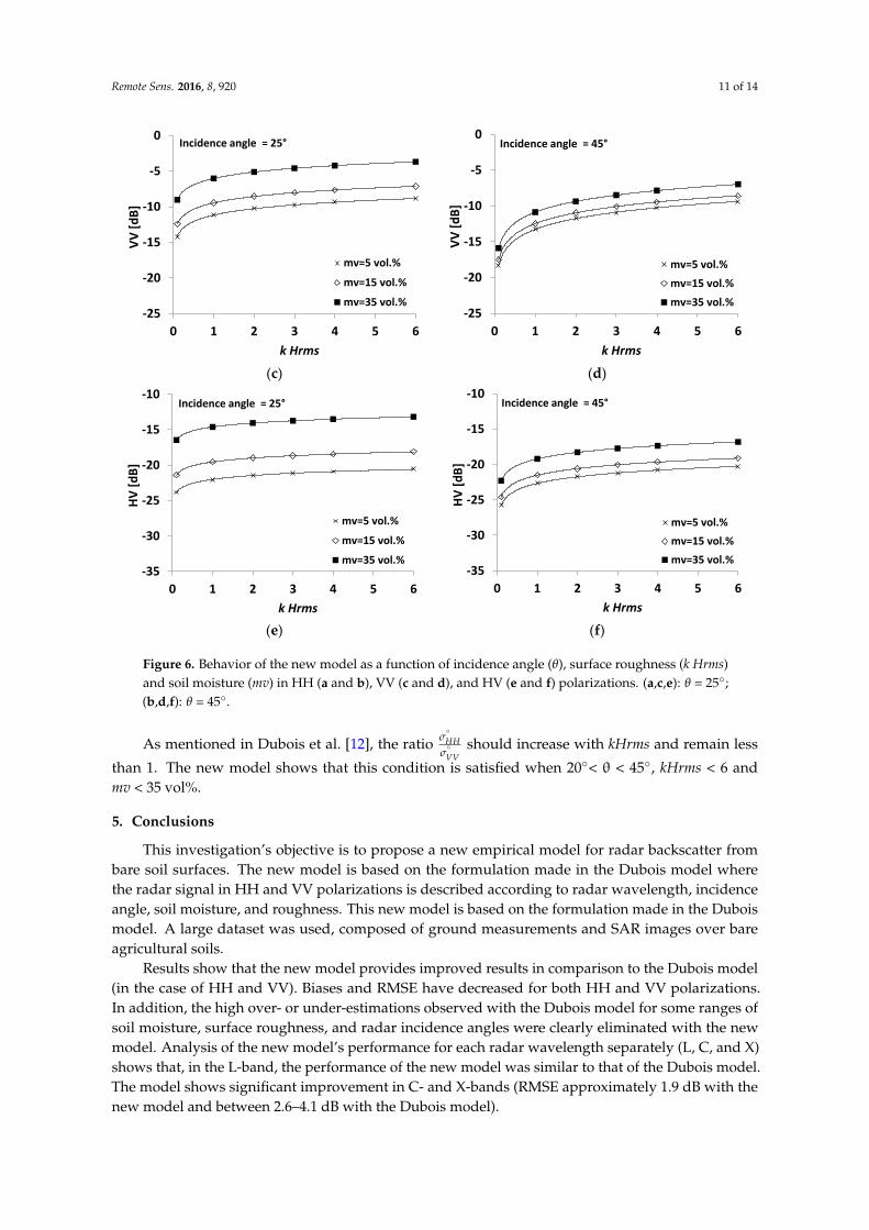
Figure 6 shows that the radar signal is strongly sensitive to surface roughness, especially forsmall values of kHrms. In addition, this sensitivity increases with the incidence angle. Concerning theinfluence of polarization, the new model shows, as do many theories and experimental studies, that agiven soil roughness leads to slightly higher signal dynamics with the soil moisture in HH than in VVpolarization [17,46]. The radar signal σ◦ increases with kHrms. This increase is higher for either lowkHrms values or high θ values than it is for either high kHrms values or low θ values. For θ = 45◦, σ◦
increases approximately 8 dB in HH and 6.5 dB in VV when kHrms increases from 0.1 to 2 comparedwith only 3 dB when kHrms increases from two to six (for both HH and VV). This dynamic of σ◦ isonly half for θ = 25◦ in comparison to that for θ = 45◦. In HV, the dynamic of σ◦ to kHrms is half thatobserved for HH and VV.
The behavior of σ◦ according to soil moisture shows a larger increase of σ◦ with mv for lowincidence angles than for high incidence angles. Figure 6 shows that σ◦
HH and σ◦VV increase
approximately 6 dB for θ = 25◦ compared with only 3 dB for θ = 45◦ when mv increases from five to35 vol%. In HV, the signal increases approximately 7.5 dB for θ = 25◦ and 3.5 dB for θ = 45◦ when mvincreases from 5 to 35 vol%.
Remote Sens. 2016, 8, 920 10 of 14
(c) (d)
Figure 5. (a) Comparison between ° in the new model and ° measured (for all SAR bands) for HV
polarization; (b) the difference between SAR and the new model as a function of kHrms; (c) the
difference between SAR and the new model as a function of mv; and (d) the difference between SAR
and the new model as a function of incidence angle. The best regression model is plotted in gray.
4.2.2. Behavior of the New Model
The physical behavior of the new radar backscatter model was studied as a function of the
incidence angle (), soil moisture (mv), and surface roughness (kHrms).
Figure 6 shows that the radar signal is strongly sensitive to surface roughness, especially for
small values of kHrms. In addition, this sensitivity increases with the incidence angle. Concerning the
influence of polarization, the new model shows, as do many theories and experimental studies, that
a given soil roughness leads to slightly higher signal dynamics with the soil moisture in HH than in
VV polarization [17,46]. The radar signal ° increases with kHrms. This increase is higher for either
low kHrms values or high values than it is for either high kHrms values or low values. For = 45°,
° increases approximately 8 dB in HH and 6.5 dB in VV when kHrms increases from 0.1 to 2
compared with only 3 dB when kHrms increases from two to six (for both HH and VV). This dynamic
of ° is only half for = 25° in comparison to that for = 45°. In HV, the dynamic of ° to kHrms is
half that observed for HH and VV.
The behavior of ° according to soil moisture shows a larger increase of ° with mv for low incidence
angles than for high incidence angles. Figure 6 shows that °HH and °VV increase approximately 6 dB for
= 25° compared with only 3 dB for = 45° when mv increases from five to 35 vol%. In HV, the signal
increases approximately 7.5 dB for = 25° and 3.5 dB for = 45° when mv increases from 5 to 35 vol%.
As mentioned in Dubois et al. [12], the ratio 𝜎𝐻𝐻°
𝜎𝑉𝑉°⁄ should increase with kHrms and remain less
than 1. The new model shows that this condition is satisfied when 20°< < 45°, kHrms < 6 and mv < 35 vol%.
(a) (b)
y = 0.01x - 0.28R² = 0.00
-15
-10
-5
0
5
10
15
0 5 10 15 20 25 30 35 40 45 50
SAR
-N
ew m
od
el [
dB
]
Soil moisture (vol. %)
L-band C-band X-band
y = 0.01x - 0.24R² = 0.00
-15
-10
-5
0
5
10
15
15 20 25 30 35 40 45 50 55 60
SAR
-N
ew m
od
el [
dB
]
Incidence angle (°)
L-band C-band X-band
-25
-20
-15
-10
-5
0
0 1 2 3 4 5 6
HH
[d
B]
k Hrms
Incidence angle = 25°
mv=5 vol.%
mv=15 vol.%
mv=35 vol.%-25
-20
-15
-10
-5
0
0 1 2 3 4 5 6
HH
[d
B]
k Hrms
Incidence angle = 45°
mv=5 vol.%
mv=15 vol.%
mv=35 vol.%
Figure 6. Cont.
Remote Sens. 2016, 8, 920 11 of 14Remote Sens. 2016, 8, 920 11 of 14
(c) (d)
(e) (f)
Figure 6. Behavior of the new model as a function of incidence angle (), surface roughness (k Hrms)
and soil moisture (mv) in HH (a and b), VV (c and d), and HV (e and f) polarizations. (a,c,e): =25°;
(b,d,f): =45°.
5. Conclusions
This investigation’s objective is to propose a new empirical model for radar backscatter from
bare soil surfaces. The new model is based on the formulation made in the Dubois model where the
radar signal in HH and VV polarizations is described according to radar wavelength, incidence angle, soil
moisture, and roughness. This new model is based on the formulation made in the Dubois model. A large
dataset was used, composed of ground measurements and SAR images over bare agricultural soils.
Results show that the new model provides improved results in comparison to the Dubois model
(in the case of HH and VV). Biases and RMSE have decreased for both HH and VV polarizations. In
addition, the high over- or under-estimations observed with the Dubois model for some ranges of
soil moisture, surface roughness, and radar incidence angles were clearly eliminated with the new
model. Analysis of the new model’s performance for each radar wavelength separately (L, C, and X)
shows that, in the L-band, the performance of the new model was similar to that of the Dubois model.
The model shows significant improvement in C- and X-bands (RMSE approximately 1.9 dB with the
new model and between 2.6–4.1 dB with the Dubois model).
Based on the same equation as that used for HH and VV, a radar signal in HV polarization was
also proposed. Finally, the new empirical model proposed in the present study would allow more
accurate soil moisture estimates using the new Sentinel-1A and -1B SAR data.
Acknowledgments: This research was supported by IRSTEA (National Research Institute of Science and
Technology for Environment and Agriculture), the French Space Study Center (CNES, TOSCA 2016) and the
Belgian Science Policy Office (Contract SR/00/302). Hans Lievens is a postdoctoral research fellow of the Research
-25
-20
-15
-10
-5
0
0 1 2 3 4 5 6
VV
[d
B]
k Hrms
Incidence angle = 25°
mv=5 vol.%
mv=15 vol.%
mv=35 vol.%-25
-20
-15
-10
-5
0
0 1 2 3 4 5 6
VV
[d
B]
k Hrms
Incidence angle = 45°
mv=5 vol.%
mv=15 vol.%
mv=35 vol.%
-35
-30
-25
-20
-15
-10
0 1 2 3 4 5 6
HV
[d
B]
k Hrms
Incidence angle = 25°
mv=5 vol.%
mv=15 vol.%
mv=35 vol.%-35
-30
-25
-20
-15
-10
0 1 2 3 4 5 6
HV
[d
B]
k Hrms
Incidence angle = 45°
mv=5 vol.%
mv=15 vol.%
mv=35 vol.%
Figure 6. Behavior of the new model as a function of incidence angle (θ), surface roughness (k Hrms)and soil moisture (mv) in HH (a and b), VV (c and d), and HV (e and f) polarizations. (a,c,e): θ = 25◦;(b,d,f): θ = 45◦.
As mentioned in Dubois et al. [12], the ratio σ◦HH
σ◦VV
should increase with kHrms and remain less
than 1. The new model shows that this condition is satisfied when 20◦< θ < 45◦, kHrms < 6 andmv < 35 vol%.
5. Conclusions
This investigation’s objective is to propose a new empirical model for radar backscatter frombare soil surfaces. The new model is based on the formulation made in the Dubois model wherethe radar signal in HH and VV polarizations is described according to radar wavelength, incidenceangle, soil moisture, and roughness. This new model is based on the formulation made in the Duboismodel. A large dataset was used, composed of ground measurements and SAR images over bareagricultural soils.
Results show that the new model provides improved results in comparison to the Dubois model(in the case of HH and VV). Biases and RMSE have decreased for both HH and VV polarizations.In addition, the high over- or under-estimations observed with the Dubois model for some ranges ofsoil moisture, surface roughness, and radar incidence angles were clearly eliminated with the newmodel. Analysis of the new model’s performance for each radar wavelength separately (L, C, and X)shows that, in the L-band, the performance of the new model was similar to that of the Dubois model.The model shows significant improvement in C- and X-bands (RMSE approximately 1.9 dB with thenew model and between 2.6–4.1 dB with the Dubois model).
Remote Sens. 2016, 8, 920 12 of 14
Based on the same equation as that used for HH and VV, a radar signal in HV polarization wasalso proposed. Finally, the new empirical model proposed in the present study would allow moreaccurate soil moisture estimates using the new Sentinel-1A and -1B SAR data.
Acknowledgments: This research was supported by IRSTEA (National Research Institute of Science andTechnology for Environment and Agriculture), the French Space Study Center (CNES, TOSCA 2016) and theBelgian Science Policy Office (Contract SR/00/302). Hans Lievens is a postdoctoral research fellow of the ResearchFoundation Flanders (FWO). Authors thank the space agencies that provided AIRSAR, SIR-C, JERS-1, ERS-1/2,RADARSAT-1/2, ASAR, PALSAR-1, TerraSAR-X, COSMO-SkyMed, and ESAR data.
Author Contributions: Nicolas Baghdadi conceived the study; Nicolas Baghdadi performed the modelingNicolas Baghdadi, Mohammad Choker and Mohammad El Hajj analyzed the results; Nicolas Baghdadi wrotethe paper; Nicolas Baghdadi, Mohammad Choker, Mehrez Zribi, Mohammad El Hajj, Simonetta Paloscia,Niko E. C. Verhoest, Hans Lievens, Frederic Baup and Francesco Mattia revised the paper.
Conflicts of Interest: The authors declare no conflict of interest.
References
1. Rao, S.S.; Kumar, S.D.; Das, S.N. Modified Dubois model for estimating soil moisture with dual polarizedSAR data. J. Indian Soc. Remote Sens. 2013, 41, 865–872.
2. Chai, X.; Zhang, T.T.; Shao, Y.; Gong, H.Z.; Liu, L.; Xie, K.X. Modeling and mapping soil moisture of plateaupasture using RADARSAT-2 imagery. Remote Sens. 2015, 7, 1279–1299.
3. Kirimi, F.; Kuria, D.N.; Frank Thonfeld, F.; Amler, E.; Mubea, K.; Misana, S.; Gunter Menz, G. Influence ofvegetation cover on the Oh soil moisture retrieval model: A case study of the Malinda Wetland, Tanzania.Adv. Remote Sens. 2016, 5, 28–42.
4. Gherboudj, I.; Magagi, R.; Berg, A.A.; Toth, B. Soil moisture retrieval over agricultural Felds frommulti-polarized and multi-angular RADARSAT-2 SAR data. Remote Sens. Environ. 2011, 115, 33–43.[CrossRef]
5. Zribi, M.; Chahbi, A.; Shabou, M.; Lili-Chabaane, Z.; Duchemin, B.; Baghdadi, N.; Amri, R.; Chehbouni, A.Soil surface moisture estimation over a semi-arid region using ENVISAT ASAR radar data for soilevaporation evaluation. Hydrol. Earth Syst. Sci. 2011, 15, 345–358. [CrossRef]
6. Le Hegarat-Mascle, S.; Zribi, M.; Alem, F.; Weisse, A.; Loumagne, C. Soil moisture estimation from ERS/SARdata: Toward an operational methodology. IEEE Trans. Geosci. Remote Sens. 2002, 40, 2647–2658. [CrossRef]
7. Zribi, M.; Dechambre, M. A new empirical model to retrieve soil moisture and roughness from Radar Data.Remote Sens. Environ. 2003, 84, 42–52. [CrossRef]
8. Oh, Y.; Sarabandi, K.; Ulaby, F.T. An empirical model and an inversion technique for radar scattering frombare soil surfaces. IEEE Trans. Geosci. Remote Sens. 1992, 30, 370–381. [CrossRef]
9. Oh, Y.; Kay, Y. Condition for precise measurement of soil surface roughness. IEEE Trans. Geosci. Remote Sens.1998, 36, 691–695.
10. Oh, Y.; Sarabandi, K.; Ulaby, F.T. Semi-empirical model of the ensemble-averaged differential Mueller matrixfor microwave backscattering from bare soil surfaces. IEEE Trans. Geosci. Remote Sens. 2002, 40, 1348–1355.[CrossRef]
11. Oh, Y. Quantitative retrieval of soil moisture content and surface roughness from multipolarized radarobservations of bare soil surfaces. IEEE Trans. Geosci. Remote Sens. 2004, 42, 596–601. [CrossRef]
12. Dubois, P.C.; Van Zyl, J.; Engman, T. Measuring soil moisture with imaging radars. IEEE Trans. Geosci.Remote Sens. 1995, 33, 915–926. [CrossRef]
13. Baghdadi, N.; Saba, E.; Aubert, M.; Zribi, M.; Baup, F. Comparison between backscattered TerraSAR signalsand simulations from the radar backscattering models IEM, Oh, and Dubois. IEEE Geosci. Remote Sens. Lett.2011, 8, 1160–1164. [CrossRef]
14. Baghdadi, N.; Zribi, M. Evaluation of radar backscatter models IEM, Oh and Dubois using experimentalobservations. Int. J. Remote Sens. 2006, 27, 3831–3852. [CrossRef]
15. Wang, H.; Méric, S.; Allain, S.; Pottier, E. Adaptation of Oh Model for soil parameters retrieval usingmulti-angular RADARSAT-2 datasets. J. Surv. Mapp. Eng. 2014, 2, 65–74.
Remote Sens. 2016, 8, 920 13 of 14
16. Wang, J.R.; Hsu, A.; Shi, J.C.; O’Neill, P.E.; Engman, E.T. A comparison of soil moisture retrieval modelsusing SIR-C measurements over the Little Washita River watershed. Remote Sens. Environ. 1997, 59, 308–320.[CrossRef]
17. Zribi, M.; Taconet, O.; Le Hégarat-Mascle, S.; Vidal-Madjar, D.; Emblanch, C.; Loumagne, C.; Normand, M.Backscattering behavior and simulation comparison over bare soils using SIRC/XSAR and ERASME 1994data over Orgeval. Remote Sens. Environ. 1997, 59, 256–266. [CrossRef]
18. Baghdadi, N.; Dubois-Fernandez, P.; Dupuis, X.; Zribi, M. Sensitivity of mail polarimetric parameters ofmultifrequency polarimetric SAR data to soil moisture and surface roughness over bare agricultural soils.IEEE Geosci. Remote Sens. Lett. 2013, 10, 731–735. [CrossRef]
19. Baghdadi, N.; Zribi, M.; Loumagne, C.; Ansart, P.; Paris Anguela, T. Analysis of TerraSAR-X data and theirsensitivity to soil surface parameters over bare agricultural fields. Remote Sens. Environ. 2008, 112, 4370–4379.[CrossRef]
20. Baghdadi, N.; Aubert, M.; Zribi, M. Use of TerraSAR-X data to retrieve soil moisture over bare soil agriculturalfields. IEEE Geosci. Remote Sens. Lett. 2012, 9, 512–516. [CrossRef]
21. Baghdadi, N.; Gherboudj, I.; Zribi, M.; Sahebi, M.; Bonn, F.; King, C. Semi-empirical calibration of the IEMbackscattering model using radar images and moisture and roughness field measurements. Int. J. RemoteSens. 2004, 25, 3593–3623. [CrossRef]
22. Baghdadi, N.; King, C.; Bourguignon, A.; Remond, A. Potential of ERS and RADARSAT data for surfaceroughness monitoring over bare agricultural fields: Application to catchments in Northern France. Int. J.Remote Sens. 2002, 23, 3427–3442. [CrossRef]
23. Holah, H.; Baghdadi, N.; Zribi, M.; Bruand, A.; King, C. Potential of ASAR/ENVISAT for the characterisationof soil surface parameters over bare agricultural fields. Remote Sens. Environ. 2005, 96, 78–86. [CrossRef]
24. Baghdadi, N.; Holah, N.; Zribi, M. Calibration of the Integral Equation Model for SAR data in C-band andHH and VV polarizations. Int. J. Remote Sens. 2006, 27, 805–816. [CrossRef]
25. Le Morvan, A.; Zribi, M.; Baghdadi, N.; Chanzy, A. Soil moisture profile effect on radar signal measurement.Remote Sens. 2008, 8, 256–270. [CrossRef]
26. Baghdadi, N.; Cresson, R.; El Hajj, M.; Ludwig, R.; La Jeunesse, I. Estimation of soil parameters over bareagriculture areas from C-band polarimetric SAR data using neural networks. Hydrol. Earth Syst. Sci. (HESS)2012, 16, 1607–1621. [CrossRef]
27. Baghdadi, N.; Aubert, M.; Cerdan, O.; Franchistéguy, L.; Viel, C.; Martin, E.; Zribi, M.; Desprats, J.F.Operational mapping of soil moisture using synthetic aperture radar data: Application to Touch basin(France). Sens. J. 2007, 7, 2458–2483. [CrossRef]
28. Zribi, M.; Gorrab, A.; Baghdadi, N.; Lili-Chabaane, Z. Influence of radar frequency on the relationshipbetween bare surface soil moisture vertical profile and radar backscatter. IEEE Geosci. Remote Sens. Lett. 2014,11, 848–852. [CrossRef]
29. Gorrab, A.; Zribi, M.; Baghdadi, N.; Mougenot, B.; Lili-Chabaane, Z. Retrieval of both soil moisture andtexture using TerraSAR-X images. Remote Sens. 2015, 7, 10098–10116. [CrossRef]
30. Aubert, M.; Baghdadi, N.; Zribi, M.; Ose, K.; El Hajj, M.; Vaudour, E.; Gonzalez-Sosa, E. Toward anoperational bare soil moisture mapping using TerraSAR-X data acquired over agricultural areas. IEEE J. Sel.Top. Appl. Earth Obs. Remote Sens. (JSTARS) 2013, 6, 900–916. [CrossRef]
31. Dong, L.; Baghdadi, N.; Ludwig, R. Retrieving surface soil moisture using radar imagery in a semi-aridenvironment. IEEE Geosci. Remote Sens. Lett. 2013, 10, 461–465. [CrossRef]
32. Baup, F.; Fieuzal, R.; Marais-Sicre, C.; Dejoux, J.-F.; le Dantec, V.; Mordelet, P.; Claverie, M.; Hagolle, O.;Lopes, A.; Keravec, P.; et al. MCM’10: An experiment for satellite multi-sensors crop monitoring. In FromHigh to Low Resolution Observations, IEEE International Geoscience and Remote Sensing Symposium,Munich, Germany, 22–27 July 2012.
33. Mattia, M.; Toan, T.L.; Souyris, J.C.; Carolis, G.D.; Floury, N.; Posa, F.; Pasquariello, G. The effect of surfaceroughness on multifrequency polarimetric SAR data. IEEE Trans. Geosci. Remote Sens. 1997, 35, 954–966.[CrossRef]
34. Lievens, H.; Verhoest, N.E.C.; De Keyser, E.; Vernieuwe, H.; Matgen, P.; Álvarez-Mozos, J.; De Baets, B.Effective roughness modelling as a tool for soil moisture retrieval from C-and L-band SAR. Hydrol. EarthSyst. Sci. 2011, 15, 151–162. [CrossRef]
Remote Sens. 2016, 8, 920 14 of 14
35. Baronti, S.; Del Frate, F.; Ferrazzoli, P.; Paloscia, S.; Pampaloni, P.; Schiavon, G. SAR polarimetric features ofagricultural areas. Int. J. Remote Sens. 1995, 16, 2639–2656. [CrossRef]
36. Macelloni, G.; Paloscia, S.; Pampaloni, P.; Sigismondi, S.; de Matthæis, P.; Ferrazzoli, P.; Schiavon, G.;Solimini, D. The SIR-C/X-SAR experiment on Montespertoli: Sensitivity to hydrological parameters. Int. J.Remote Sens. 1999, 20, 2597–2612. [CrossRef]
37. Paloscia, S.; Macelloni, G.; Pampaloni, P.; Sigismondi, S. The potential of C- and L-band SAR in estimatingvegetation biomass: The ERS-1 and JERS-1 Experiments. IEEE Trans. Geosci. Remote Sens. 1999, 37, 2107–2110.[CrossRef]
38. Ulaby, F.T.; Moore, R.K.; Fung, A.K. Microwave Remote Sensing; Addison-Wesley: New York, NY, USA, 1982.39. Beauchemin, M.; Thomson, K.; Edwards, G. Modelling forest stands with MIMICS: Implications for
calibration. Can. J. Remote Sens. 1995, 21, 518–526. [CrossRef]40. Baghdadi, N.; Bernier, M.; Gauthier, R.; Neeson, I. Evaluation of C-band SAR data for wetlands mapping.
Int. J. Remote Sens. 2001, 22, 71–88. [CrossRef]41. Baghdadi, N.; Holah, N.; Zribi, M. Soil moisture estimation using multi-incidence and multi-polarization
ASAR SAR data. Int. J. Remote Sens. 2006, 27, 1907–1920. [CrossRef]42. Aubert, M.; Baghdadi, N.; Zribi, M.; Douaoui, A.; Loumagne, C.; Baup, F.; El Hajj, M.; Garrigues, S.
Characterization of soil surface by TerraSAR-X imagery. Remote Sens. Environ. 2011, 115, 1801–1810.[CrossRef]
43. Baghdadi, N.; Cerdan, O.; Zribi, M.; Auzet, V.; Darboux, F.; El Hajj, M.; Bou Kheir, R. Operationalperformance of current synthetic aperture radar sensors in mapping soil surface characteristics in agriculturalenvironments: Application to hydrological and erosion modelling. Hydrol. Process. 2008, 22, 9–20. [CrossRef]
44. Srivastava, H.S.; Patel, P.; Manchanda, M.L.; Adiga, S. Use of multi-incidence angle RADARSAT-1 SAR datato incorporate the effects of surface roughness in soil moisture estimation. IEEE Trans. Geosci. Remote Sens.2003, 41, 1638–1640. [CrossRef]
45. Sahebi, M.R.; Angles, J.; Bonn, F. A comparison of multi-polarization and multi-angular approaches forestimating bare soil surface roughness from spaceborne radar data. Can. J. Remote Sens. 2002, 28, 641–652.[CrossRef]
46. Fung, A.K. Microwave Scattering and Emission Models and Their Applications; Artech House, Inc.: Boston, MA,USA, 1994.
© 2016 by the authors; licensee MDPI, Basel, Switzerland. This article is an open accessarticle distributed under the terms and conditions of the Creative Commons Attribution(CC-BY) license (http://creativecommons.org/licenses/by/4.0/).