fluids

Article

A New Exact Solution for the Flow of a Fluid throughPorous Media for a Variety of Boundary Conditions

U. S. Mahabaleshwar 1, P. N. Vinay Kumar 2,* , K. R. Nagaraju 3, Gabriella Bognár 4

and S. N. Ravichandra Nayakar 5

1 Department of Mathematics, Davangere University, Shivagangothri, Davangere 577 007, India2 Department of Mathematics, SHDD Government First Grade College, Paduvalahippe, Hassan 573 211, India3 Department of Mathematics, Government Engineering College, Hassan 573 201, India4 Faculty of Mechanical Engineering and Informatics, Institute of Machine and Product Design,

University of Miskolc, 3515 Miskolc-Egyetemvaros, Hungary5 Department of Mathematics, University BDT College of Engineering, Davangere 577 004, India* Correspondence: vinaykumarpn1981@gmail.com

Received: 23 May 2019; Accepted: 29 June 2019; Published: 8 July 2019�����������������

Abstract: The viscous fluid flow past a semi-infinite porous solid, which is proportionally sheared atone boundary with the possibility of the fluid slipping according to Navier’s slip or second order slip,is considered here. Such an assumption takes into consideration several of the boundary conditionsused in the literature, and is a generalization of them. Upon introducing a similarity transformation,the governing equations for the problem under consideration reduces to a system of nonlinear partialdifferential equations. Interestingly, we were able to obtain an exact analytical solution for the velocity,though the equation is nonlinear. The flow through the porous solid is assumed to obey the Brinkmanequation, and is considered relevant to several applications.

Keywords: Brinkman equation; viscosity ratio; first- and second-order slip; similarity transformation;porous medium

1. Introduction

The flow of a fluid through a porous medium has numerous applications in industries dealingwith polymer extrusion process, glass blowing, metallurgical processes, and geophysical and alliedareas (see [1]). A variety of equations have been used to describe the flow of a fluid through a porousmedium as it is one of the important key factors in maintaining the temperature in the medium.These equations due to [2–5] and others, are merely approximations to the appropriate balance laws.A variety of ideas have been suggested to model the flow of mixtures, and one such approach isthat which follows from the seminal works of Darcy and Brinkman and has been given a formalstructure by [6,7]. Several specific problems have been solved using such an approach (see [8–19]).Here, we study the flow of a fluid through a porous media that is governed by the Brinkman equation(see [20–30]) for a discussion of the status of the Brinkman equation within the context of mixturetheory). The fact that we are able to obtain an analytical solution to the problem makes the studyall the more interesting. Despite the fact that advanced computing facilities are available to obtainthe numerical solution, investigators around the world are much more interested in providing theanalytical solution due to their accuracy, relevance, and convenient to analyze physical process,in comparison to numerical solutions. The analytical solution can provide a better assessment ofconsistency and parameter estimates. Many authors have investigated the fluid flow through porousmedia and provided analytical solution (see [31–37]). The novelty of this study is our use of a variety

Fluids 2019, 4, 125; doi:10.3390/fluids4030125 www.mdpi.com/journal/fluids

Fluids 2019, 4, 125 2 of 22

of boundary conditions that subsumes those that have been considered earlier, in addition to newconditions concerning slip and proportional shearing at the boundary.

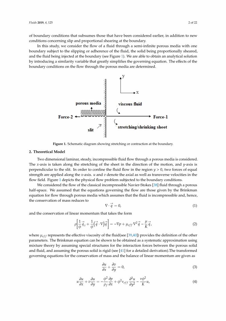
In this study, we consider the flow of a fluid through a semi-infinite porous media with oneboundary subject to the slipping or adherence of the fluid, the solid being proportionally sheared,and the fluid being injected at the boundary (see Figure 1). We are able to obtain an analytical solutionby introducing a similarity variable that greatly simplifies the governing equation. The effects of theboundary conditions on the flow through the porous media are determined.

Fluids 2019, 4, x FOR PEER REVIEW 2 of 22

conditions that subsumes those that have been considered earlier, in addition to new conditions concerning slip and proportional shearing at the boundary.

In this study, we consider the flow of a fluid through a semi-infinite porous media with one boundary subject to the slipping or adherence of the fluid, the solid being proportionally sheared, and the fluid being injected at the boundary (see Figure 1). We are able to obtain an analytical solution by introducing a similarity variable that greatly simplifies the governing equation. The effects of the boundary conditions on the flow through the porous media are determined.

Figure 1. Schematic diagram showing stretching or contraction at the boundary.

2. Theoretical Model

Two dimensional laminar, steady, incompressible fluid flow through a porous media is considered. The x-axis is taken along the stretching of the sheet in the direction of the motion, and y-axis is perpendicular to the slit. In order to confine the fluid flow in the region y>0, two forces of equal strength are applied along the x-axis. u and v denote the axial as well as transverse velocities in the flow field. Figure 1 depicts the physical flow problem subjected to the boundary conditions.

We considered the flow of the classical incompressible Navier-Stokes [38] fluid through a porous half-space. We assumed that the equations governing the flow are those given by the Brinkman equation for flow through porous media which assumes that the fluid is incompressible and, hence, the conservation of mass reduces to

0q =∇ ⋅ , (1)

and the conservation of linear momentum that takes the form

( ) 2 ,1 1t effq q q p q q

Kρ μμ

φ φ⋅∇ = −∇ ∇ −

+ +

(2)

where effμ represents the effective viscosity of the fluid(see [39,40]) provides the definition of the

other parameters. The Brinkman equation can be shown to be obtained as a systematic approximation using mixture theory by assuming special structures for the interaction forces between the porous solid and fluid, and assuming the porous solid is rigid (see[41] for a detailed derivation).The transformed governing equations for the conservation of mass and the balance of linear momentum are given as

0u vx y

∂ ∂+ =∂ ∂

, (3)

2 22

2

2 ,efff

u u p uu v ux y x y K

φ νφφ νρ

∂ ∂ ∂ ∂+ = − + −∂ ∂ ∂ ∂

(4)

Figure 1. Schematic diagram showing stretching or contraction at the boundary.

2. Theoretical Model

Two dimensional laminar, steady, incompressible fluid flow through a porous media is considered.The x-axis is taken along the stretching of the sheet in the direction of the motion, and y-axis isperpendicular to the slit. In order to confine the fluid flow in the region y > 0, two forces of equalstrength are applied along the x-axis. u and v denote the axial as well as transverse velocities in theflow field. Figure 1 depicts the physical flow problem subjected to the boundary conditions.

We considered the flow of the classical incompressible Navier-Stokes [38] fluid through a poroushalf-space. We assumed that the equations governing the flow are those given by the Brinkmanequation for flow through porous media which assumes that the fluid is incompressible and, hence,the conservation of mass reduces to

∇ ·→q = 0, (1)

and the conservation of linear momentum that takes the form

ρ

[1φ

→q t +

1φ

(→q · ∇

)→q]= −∇p + µe f f ∇

2→q −µ

K→q , (2)

where µe f f represents the effective viscosity of the fluid(see [39,40]) provides the definition of the otherparameters. The Brinkman equation can be shown to be obtained as a systematic approximation usingmixture theory by assuming special structures for the interaction forces between the porous solidand fluid, and assuming the porous solid is rigid (see [41] for a detailed derivation).The transformedgoverning equations for the conservation of mass and the balance of linear momentum are given as

∂u∂x

+∂v∂y

= 0, (3)

u∂u∂x

+ v∂u∂y

= −φ2

ρ f

∂p∂x

+ φ2νe f f∂2u∂y2 −

νφ2

Ku, (4)

Fluids 2019, 4, 125 3 of 22

where ν = µρ f

and νe f f =µe f fρ f

. The Forchheimer term in the interaction is neglected as it produces littleimpact on the fluid flow in a porous medium governed by the Brinkman equation (see [42]). Also,the pressure gradient is neglected, and the time factor is zero for the steady case.

The governing boundary conditions are (see [43,44])

Here, d is the parameter of proportional shearing at the boundary, with d , 0 and d = 0 correspondingto the boundary at y = 0 and being either proportionally sheared or being fixed. The constants A andB represent the first- and second-order slip coefficients, respectively. Also, the mass transpirationparameter, vc, represents suction or injection depending on vc > 0 or vc < 0, respectively.

In order to carry out the analysis, the physical stream functions in terms of similarity variables fand η are introduced as follows:

ψ =√α νe f f x f (η), (6)

where

η =1φ

√ανe f f

y. (7)

In terms of physical stream function ψ, the axial and transverse velocities can be rewrittenas follows:

u =∂ψ

∂y, v = −

∂ψ

∂x. (8)

The Equation (8) satisfies the continuity equation. Upon substitution of Equations (6) and (7) intoEquation (4), we obtain

Λ∂3ψ

∂y3 +∂(ψ, ∂ψ∂y )

∂(x, y)−K1

∂ψ

∂y= 0. (9)

Here, the second term indicates the Jacobian and subject. The appropriate boundary conditions are(see [43,44]) as follows:

∂ψ

∂y= dαx + A

∂u∂y

+ B∂2u∂y2 ,

∂ψ

∂x= vc at y = 0, (10a)

∂ψ

∂y= 0, as y→∞. (10b)

Here, Λ =µe f fµ is the Brinkman number or viscosity ratio. Using Equations (9) and (10) with

Equation (6), the following transformed equation with constant coefficient is derived:

Λ fηηη + f fηη − f 2η −K1 fη = 0. (11)

The governing boundary conditions for Equation (11) are given as

f (0) = Vc, fη(0) = d + Γ1 fηη(0) + Γ2 fηηη(0), at η = 0, (12)

fη(∞)→ 0 as η→∞, (13)

Fluids 2019, 4, 125 4 of 22

where Γ1 = A√αν > 0 and Γ2 = Bα

ν < 0 are the first- and second-order slip parameters, and K1 =νφ2

αK is

the reciprocal of Darcy number Da = l2K , with l = φ

√να and Vc =

vc√αρ as the mass suction/injection

parameters. The subscript denotes the derivative with respect to η.

3. The Analytical Solution

The flow problem considered is the generalization of the classical works of [43–48]. In our problem,the viscous flow with first- and second-order velocity slips over a porous half-space that is stretched orcontracted at the boundary (see Figure 1), and the flow being governed by the Darcy–Brinkman modelis considered. One obtains nonlinear partial differentiation from Equations (3) and (4), which aremapped into systems of the nonlinear ordinary differential Equation (11), with a constant coefficientby means of similarity transformation subjected to the imposed boundary (12)–(13).The analyticalsolution for the velocity distribution is determined.

The exact analytical solution of Equation (11) subjected to the governing boundary conditionsEquations (12) and (13) is derived. The condition in Equation (13) suggests choosing the equation ofthe form

f (η) = A1 + B1 exp(−βη), (14)

where β > 0 is to be determined later. Also, A1 and B1 are constants that are to be determined by usingEquation (12):

A1 = Vc + d(

1β+ Γ1β2 − Γ2β3

)and B1 = −d

(1

β+ Γ1β2 − Γ2β3

). (15)

It follows from Equation (11), (14), and (15) that

ΛΓ2β4− (Λ Γ1 + VcΓ2)β

3 + (VcΓ1 −Λ −K1Γ2)β2 + (Vc + K1Γ1)β− (d + K1) = 0. (16)

Here, β > 0 is one of the real roots (see [49,50]).By using the transformation variable ξ = β+ a3

4 , Equation (16) transforms into

ξ4 + p ξ2 + q ξ+ r = 0, (17)

where p = a2 −38 a2

3, q =(A1 −

12 A2A3 +

18 A3

3

), and r = a0 −

14 a1a3 +

116 a2a2

3 −3

256 a43, and a3 = −Λ Γ1+VcΓ2

ΛΓ2,

a2 = VcΓ1−Λ−K1Γ2ΛΓ2

, a1 = Vc+K1Γ1ΛΓ2

, a0 = d+K1ΛΓ2

.The four corresponding roots of the algebraic Equation (17) are

β1 =

√C

2+

12

√D1 −

a3

4, (18a)

β2 =

√C

2−

12

√D1 −

a3

4, (18b)

β3 = −

√C

2+

12

√D1 −

a3

4, (18c)

β4 = −

√C

2−

12

√D1 −

a3

4, (18d)

where

D1 = D−2qC

,

C = −2p3 + 21/3

(p2 + 12r

)3(2p3 + 27q2− 72pr +

√−4(p2 + 12r)3 + (2p3 + 27q2 − 72pr)2

)1/3−1

+(21/3 3

)−1(2p3 + 27q2

− 72pr +√−4(p2 + 12r)3 + (2p3 + 27q2 − 72pr)2

)1/3

Fluids 2019, 4, 125 5 of 22

and

D = −4p3 − 21/3

(p2 + 12r

)3(2p3 + 27q2− 72pr−

√−4(p2 + 12r)3 + (2p3 + 27q2 − 72pr)2

)1/3−1

−

(21/3 3

)−1(2p3 + 27q2

− 72pr +√−4(p2 + 12r)3 + (2p3 + 27q2 − 72pr)2

)1/3

Equation (18) gives the complete solution of Equation (17). However, it should be noted thatthere is only one feasible solution for the Equation (17) when Γ2 < 0, and based on the flow fieldEquation (16) has feasible solutions for β > 0.

4. Results and Discussion

In this paper, we were able to establish the impact of various physical parameters on the velocitydistribution. The solutions obtained are in good agreement with that of the classical works whensuitably restricted to specific conditions. The main emphasis of this study is the effect of boundaryconditions on the flow through porous media. There are several possibilities at the boundaries, namely,the fluid meeting the no-slip adherence condition, the Navier slip condition, the second-order slipcondition, as well as the possibility of blowing of the fluid.

The effects of physical parameters such as the mass transpiration parameter (VC), first-orderNavier slip (Γ1), second-order slip (Γ2),Brinkman ratio (Λ), and proportional shearing parameter(K1)are discussed graphically. As the velocity distribution is an exponential function with a negativeargument, it decreases with the increase in η. Since β is a function of mass transpiration parameter(VC), first-order Navier slip (Γ1), second-order slip (Γ2), Brinkman ratio (Λ), and proportional shearingparameter (K1)both axial as well as transverse velocities are forced to decrease exponentially.

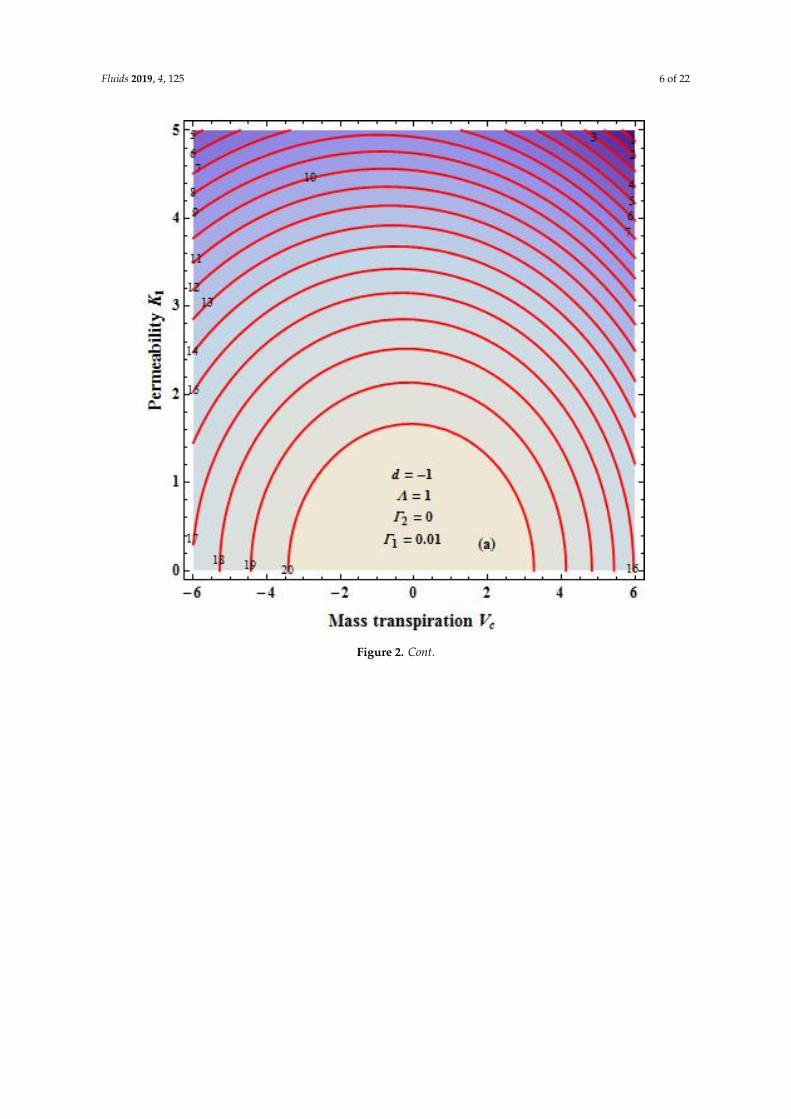
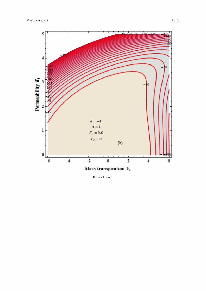
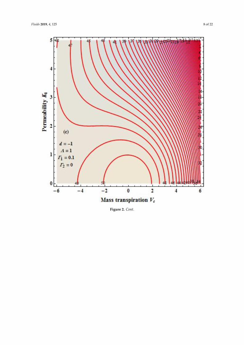
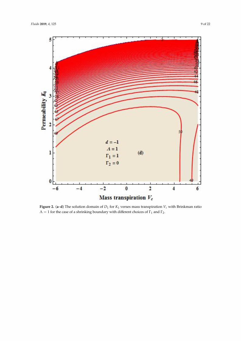
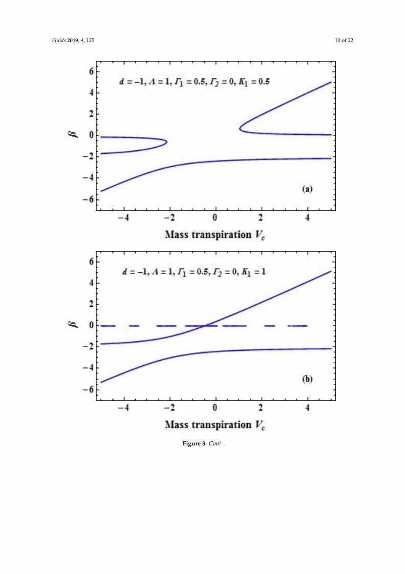
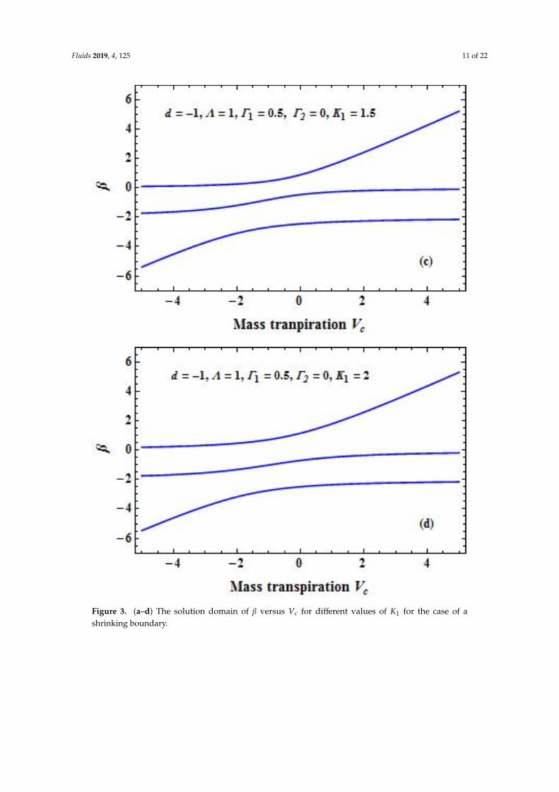
The solution domain of β in Equation (16)has only complex roots when D1 < 0, only real rootswhen D1 > 0,and real repeated roots when D1 = 0. Figure 2a–d depicts the solution behavior of βverses VC for various values of D1 and Γ1. Figure 3a–d depicts the solution domain of β versus VC fordifferent values of K1. In fact, by choosing Γ2 = 0, Equation (16) reduces to a cubic equation and withthe proper choice of Γ1, Λ, and K1, and the results are reduced to those obtained by [43,51,52].

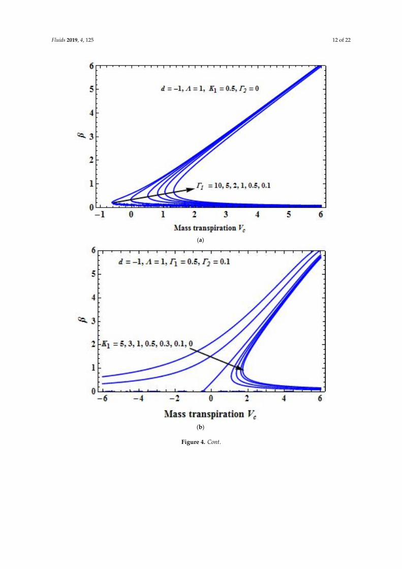
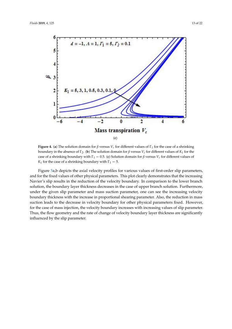
Figure 4a–c demonstrates the impact of first-order velocity slip with proportional shearing on thesolution domain of β versus Vc. The presence of a larger slip drags the separation curve towards theslit. The viscous fluid flow in a permeable medium with slip in a stretching boundary is quite differentfrom that of a contracting boundary.

Fluids 2019, 4, 125 6 of 22

Fluids 2019, 4, x FOR PEER REVIEW 6 of 22

verses CV for various values of 1D and 1Γ . Figure 3a–d depicts the solution domain of β versus CVfor different values of 1K . In fact, by choosing 2 0Γ = , Equation(16) reduces to a cubic equation and

with the proper choice of 1Γ , Λ, and 1K , and the results are reduced to those obtained by [43,51,52].

Figure 2. Cont.

Fluids 2019, 4, 125 7 of 22

Fluids 2019, 4, x FOR PEER REVIEW 7 of 22

Figure 2. Cont.

Fluids 2019, 4, 125 8 of 22

Fluids 2019, 4, x FOR PEER REVIEW 8 of 22

Figure 2. Cont.

Fluids 2019, 4, 125 9 of 22

Fluids 2019, 4, x FOR PEER REVIEW 9 of 22

Figure 2. (a–d)The solution domain of D1 for K1 verses mass transpiration Vc with Brinkman ratio

1Λ= for the case of a shrinking boundary with different choices of 1Γ and 2Γ .

Figure 2. (a–d) The solution domain of D1 for K1 verses mass transpiration Vc with Brinkman ratioΛ = 1 for the case of a shrinking boundary with different choices of Γ1 and Γ2.

Fluids 2019, 4, 125 10 of 22Fluids 2019, 4, x FOR PEER REVIEW 10 of 22

Figure 3. Cont.

Fluids 2019, 4, 125 11 of 22Fluids 2019, 4, x FOR PEER REVIEW 11 of 22

Figure 3. (a–d) The solution domain of β versus Vc for different values ofK1forthe case of a shrinking boundary.

Figure 4a–c demonstrates the impact of first-order velocity slip with proportional shearing on the solution domain of β versus Vc. The presence of a larger slip drags the separation curve towards

Figure 3. (a–d) The solution domain of β versus Vc for different values of K1 for the case of ashrinking boundary.

Fluids 2019, 4, 125 12 of 22

Fluids 2019, 4, x FOR PEER REVIEW 12 of 22

the slit. The viscous fluid flow in a permeable medium with slip in a stretching boundary is quite different from that of a contracting boundary.

(a)

(b)

Figure 4. Cont.

Fluids 2019, 4, 125 13 of 22Fluids 2019, 4, x FOR PEER REVIEW 13 of 22

(c)

Figure 4. (a)The solution domain for β versus Vc for different values of 1Γ for the case of a shrinking

boundary in the absence of 2Γ . (b)The solution domain for β versus Vc for different values of K1 for

the case of a shrinking boundary with 1 0.5Γ = . (c) Solution domain for β versus Vc for different

values of K1for the case of a shrinking boundary with 1 5Γ = .

Figure 5a,b depicts the axial velocity profiles for various values of first-order slip parameters, and for the fixed values of other physical parameters. This plot clearly demonstrates that the increasing Navier’s slip results in the reduction of the velocity boundary. In comparison to the lower branch solution, the boundary layer thickness decreases in the case of upper branch solution. Furthermore, under the given slip parameter and mass suction parameter, one can see the increasing velocity boundary thickness with the increase in proportional shearing parameter. Also, the reduction in mass suction leads to the decrease in velocity boundary for other physical parameters fixed. However, for the case of mass injection, the velocity boundary increases with increasing values of slip parameter. Thus, the flow geometry and the rate of change of velocity boundary layer thickness are significantly influenced by the slip parameter.

Figure 4. (a) The solution domain for β versus Vc for different values of Γ1 for the case of a shrinkingboundary in the absence of Γ2. (b) The solution domain for β versus Vc for different values of K1 for thecase of a shrinking boundary with Γ1 = 0.5. (c) Solution domain for β versus Vc for different values ofK1 for the case of a shrinking boundary with Γ1 = 5.

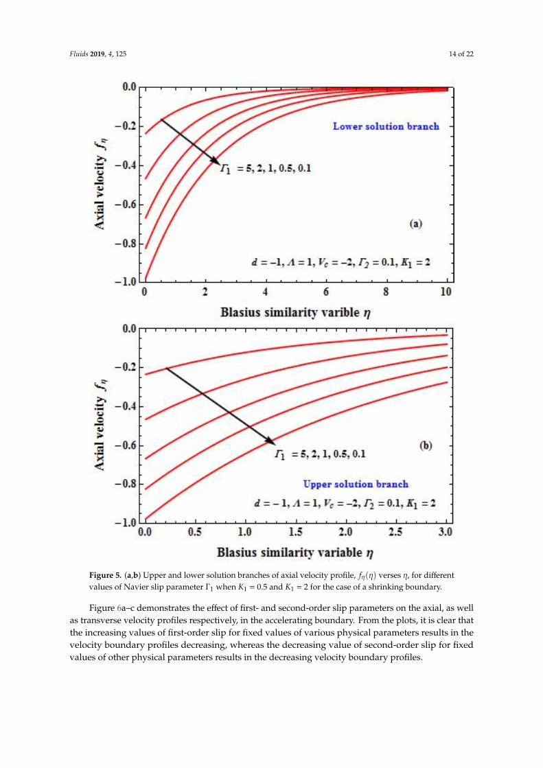
Figure 5a,b depicts the axial velocity profiles for various values of first-order slip parameters,and for the fixed values of other physical parameters. This plot clearly demonstrates that the increasingNavier’s slip results in the reduction of the velocity boundary. In comparison to the lower branchsolution, the boundary layer thickness decreases in the case of upper branch solution. Furthermore,under the given slip parameter and mass suction parameter, one can see the increasing velocityboundary thickness with the increase in proportional shearing parameter. Also, the reduction in masssuction leads to the decrease in velocity boundary for other physical parameters fixed. However,for the case of mass injection, the velocity boundary increases with increasing values of slip parameter.Thus, the flow geometry and the rate of change of velocity boundary layer thickness are significantlyinfluenced by the slip parameter.

Fluids 2019, 4, 125 14 of 22

Fluids 2019, 4, x FOR PEER REVIEW 14 of 22

Figure 5. (a,b) Upper and lower solution branches of axial velocity profile, ( )fη η verses η , for

different values of Navier slip parameter 1Γ when K1 = 0.5 and K1 =2 for the case of a shrinking

boundary.

Figure 6a–c demonstrates the effect of first- and second-order slip parameters on the axial, as well as transverse velocity profiles respectively, in the accelerating boundary. From the plots, it is clear that the increasing values of first-order slip for fixed values of various physical parameters

Figure 5. (a,b) Upper and lower solution branches of axial velocity profile, fη(η) verses η, for differentvalues of Navier slip parameter Γ1 when K1 = 0.5 and K1 = 2 for the case of a shrinking boundary.

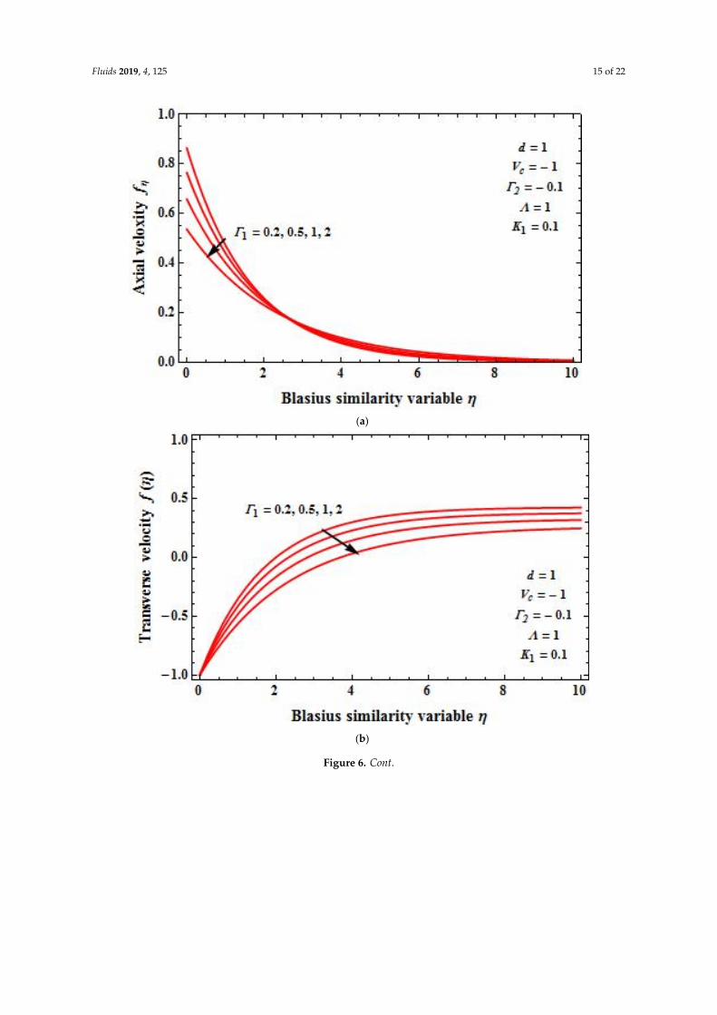
Figure 6a–c demonstrates the effect of first- and second-order slip parameters on the axial, as wellas transverse velocity profiles respectively, in the accelerating boundary. From the plots, it is clear thatthe increasing values of first-order slip for fixed values of various physical parameters results in thevelocity boundary profiles decreasing, whereas the decreasing value of second-order slip for fixedvalues of other physical parameters results in the decreasing velocity boundary profiles.

Fluids 2019, 4, 125 15 of 22

Fluids 2019, 4, x FOR PEER REVIEW 15 of 22

results in the velocity boundary profiles decreasing, whereas the decreasing value of second-order slip for fixed values of other physical parameters results in the decreasing velocity boundary profiles.

(a)

(b)

Figure 6. Cont.

Fluids 2019, 4, 125 16 of 22Fluids 2019, 4, x FOR PEER REVIEW 16 of 22

(c)

Figure 6. (a) Axial velocity ( )fη η versesη for different values of 1Γ for the case of a stretching

boundary. (b) Transverse velocity ( )f η verses η for different values of 1Γ with 2 0.1Γ =−

in the presenceofK1for the case of a stretching boundary. (c) Axial velocity ( )fη η verses η for

different values of 2Γ with 1 0.5Γ = in the presenceofK1for the case of a stretching boundary.

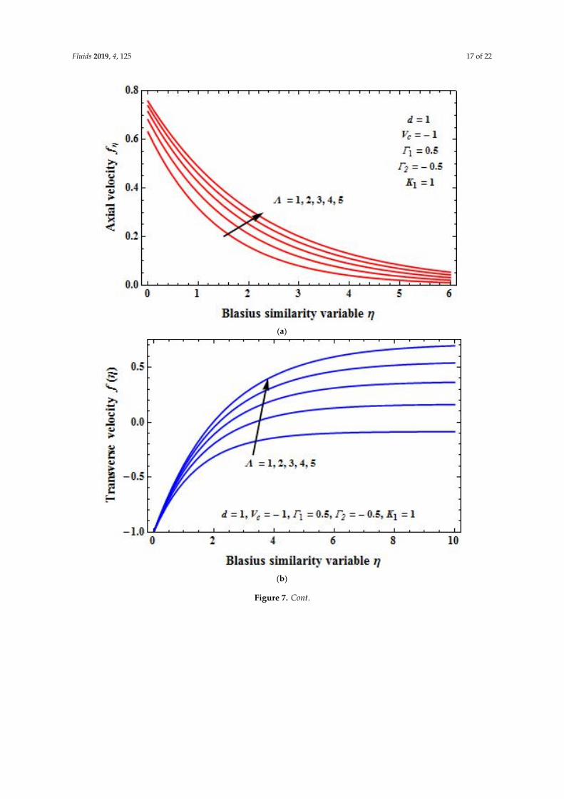
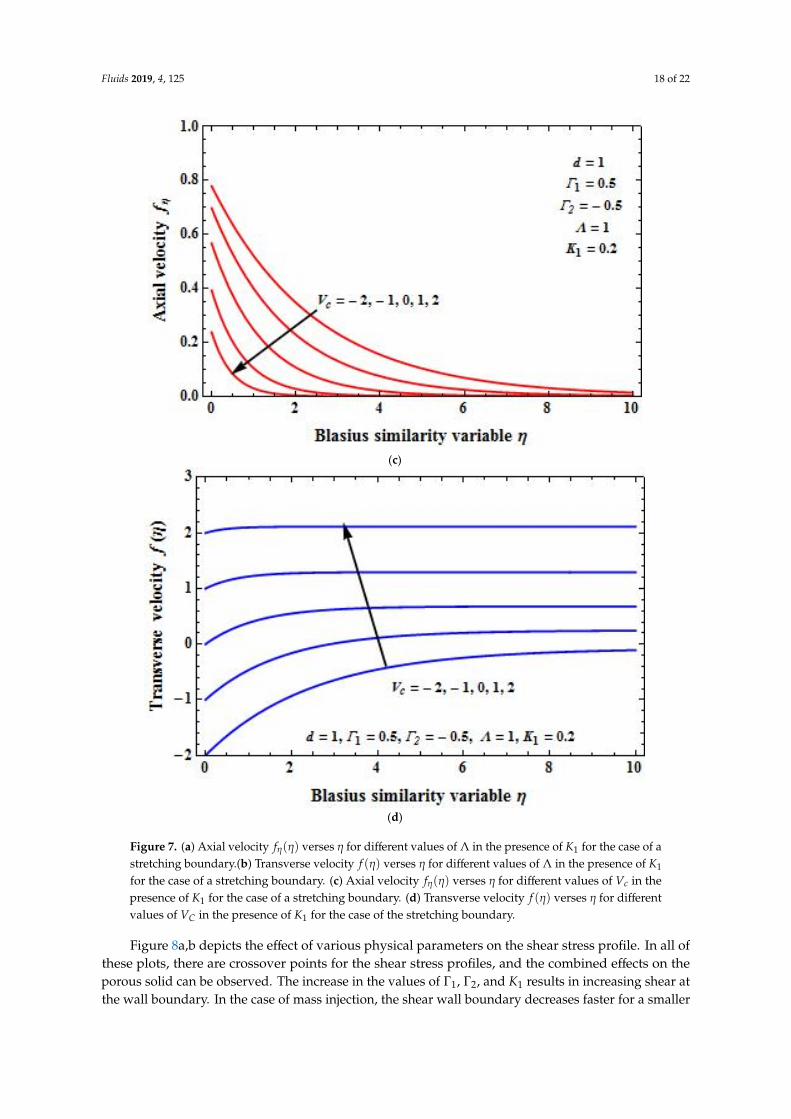
Figure 7a,b demonstrates the effect of Brinkman ratio on the axial and transverse velocity profiles. From the plots, it can be seen that increasing values of Λ while keeping other physical parameters fixed results in enhanced boundary layer thickness, whereas in Figure 7c,d, the different values of VC with fixed Brinkman ratio result in exactly the opposite.

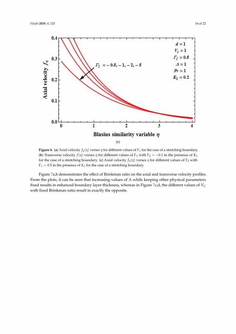
Figure 6. (a) Axial velocity fη(η) verses η for different values of Γ1 for the case of a stretching boundary.(b) Transverse velocity f (η) verses η for different values of Γ1 with Γ2 = −0.1 in the presence of K1

for the case of a stretching boundary. (c) Axial velocity fη(η) verses η for different values of Γ2 withΓ1 = 0.5 in the presence of K1 for the case of a stretching boundary.

Figure 7a,b demonstrates the effect of Brinkman ratio on the axial and transverse velocity profiles.From the plots, it can be seen that increasing values of Λ while keeping other physical parametersfixed results in enhanced boundary layer thickness, whereas in Figure 7c,d, the different values of VCwith fixed Brinkman ratio result in exactly the opposite.

Fluids 2019, 4, 125 17 of 22Fluids 2019, 4, x FOR PEER REVIEW 17 of 22

(a)

(b)

Figure 7. Cont.

Fluids 2019, 4, 125 18 of 22Fluids 2019, 4, x FOR PEER REVIEW 18 of 22

(c)

(d)

Figure 7. (a)Axial velocity ( )fη η versesη for different values of Λ in the presenceofK1for the case of

a stretching boundary.(b) Transverse velocity ( )f η verses η for different values of Λ in the

presence of K1for the case of a stretching boundary. (c) Axial velocity ( )fη η verses η for different

values of Vc in the presence of K1for the case of a stretching boundary. (d) Transverse velocity ( )f η

verses η for different values of VC in the presence of K1for the case of the stretching boundary.

Figure 7. (a) Axial velocity fη(η) verses η for different values of Λ in the presence of K1 for the case of astretching boundary.(b) Transverse velocity f (η) verses η for different values of Λ in the presence of K1

for the case of a stretching boundary. (c) Axial velocity fη(η) verses η for different values of Vc in thepresence of K1 for the case of a stretching boundary. (d) Transverse velocity f (η) verses η for differentvalues of VC in the presence of K1 for the case of the stretching boundary.

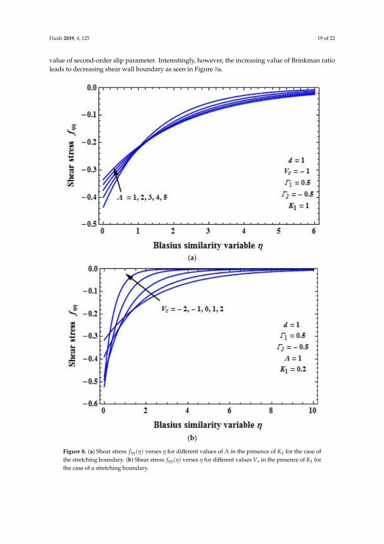
Figure 8a,b depicts the effect of various physical parameters on the shear stress profile. In all ofthese plots, there are crossover points for the shear stress profiles, and the combined effects on theporous solid can be observed. The increase in the values of Γ1, Γ2, and K1 results in increasing shear atthe wall boundary. In the case of mass injection, the shear wall boundary decreases faster for a smaller

Fluids 2019, 4, 125 19 of 22

value of second-order slip parameter. Interestingly, however, the increasing value of Brinkman ratioleads to decreasing shear wall boundary as seen in Figure 8a.

Fluids 2019, 4, x FOR PEER REVIEW 19 of 22

Figure 8a,b depicts the effect of various physical parameters on the shear stress profile. In all of these plots, there are crossover points for the shear stress profiles, and the combined effects on the

porous solid can be observed. The increase in the values of 1Γ , 2Γ , and K1 results in increasing shear at the wall boundary. In the case of mass injection, the shear wall boundary decreases faster for a smaller value of second-order slip parameter. Interestingly, however, the increasing value of Brinkman ratio leads to decreasing shear wall boundary as seen in Figure 8a.

(a)

(b)

Figure 8. (a) Shear stress fηη(η) verses η for different values of Λ in the presence of K1 for the case ofthe stretching boundary. (b) Shear stress fηη(η) verses η for different values Vc in the presence of K1 forthe case of a stretching boundary.

Fluids 2019, 4, 125 20 of 22

5. Concluding Remarks

In conclusion, the viscous fluid flow past a porous solid wherein the flow is governed by theBrinkman equation with first- and second-order slip in the presence of mass transpiration wassolved, and the exact analytical solution for the governing nonlinear partial differential equation wasobtained. The solution was analyzed for the effect of slip parameters, the mass transpiration parameter,the Brinkman ratio, and the extent of shearing or contraction. In the case of the boundary contracting,the solution branches (Figure 5a,b), whereas in the case of the boundary stretching there is only onebranch of the solution, and depending on the mass transpiration parameter, the solution is branched(Figure 5a,b).

Author Contributions: Conceptualization, U.S.M., P.N.V.K. and K.R.N.; methodology, U.S.M. and G.B.; software,P.N.V.K., K.R.N., G.B. and S.N.R.N.; validation, G.B; formal analysis, U.S.M., P.N.V.K. and K.R.N.; investigation,K.R.N.; resources, S.N.R.N.; data curation, K.R.N.; writing—original draft preparation, U.S.M., P.N.V.K., K.R.N.and S.N.R.N.; writing—review and editing, P.N.V.K. and G.B.; visualization, G.B. and S.N.R.N.; supervision,U.S.M.; project administration, U.S.M.; funding acquisition, U.S.M.

Funding: This research received no external funding.

Acknowledgments: Author K.R. Nagaraju would like to thank Sri Karisiddappa, Hon’ble Vice-chancellor, VTU,Belagavi, India (Former Principal of Government Engineering College, Hassan-573 201, India) for his valuablesupport in carrying out his research work.

Conflicts of Interest: The authors declare no conflict of interest.

References

1. Fisher, B.G. Extrusion of Plastics, 3rd ed.; Newnes-Butterworld: London, UK, 1976.2. Brinkman, H.C. On the permeability of the media consisting of closely packed porousparticles. Appl. Sci. Res.

1947, 1, 81–86. [CrossRef]3. Darcy, H. Les Fontaines Publiques De La Ville De Dijon; Victor Dalmont: Paris, France, 1856.4. Forchheimer, P. Wasserbewegung Durch Boden; Zeitschrift des Vereines Deutscher In-Geneieure:

Düsseldorf, Germany, 1901; Volume 45, pp. 1782–1788.5. Biot, M.A. Mechanics of Deformation and Acoustic Propagation in Porous Media. J. Appl. Phys. 1962, 33,

1482–1498. [CrossRef]6. Truesdell, C. Sulla basi della thermomechanical. Rend. Lincei 1957, 22a, 158–166.7. Truesdell, C. Sulla basi della thermomechanical. Rend. Lincei 1957, 22b, 33–38.8. Chakrabarti, A.; Gupta, A.S. Hydromagnetic flow and heat transfer over a stretching sheet. Q. Appl. Math.

1979, 37, 73–78. [CrossRef]9. Gupta, P.S.; Gupta, A.S. Heat and mass transfer on a stretching sheet with suction or blowing. Can. J.

Chem. Eng. 1977, 55, 744–746. [CrossRef]10. Fang, T. Boundary layer flow over a shrinking sheet with power-law velocity. Int. J. Heat Mass Transf. 2008,

51, 5838–5843. [CrossRef]11. Milavcic, M.; Wang, C.Y. Viscous flow due to a shrinking sheet. Q. Appl. Math. 2006, 64, 283–290. [CrossRef]12. Nakayama, A. PC-Aided Numerical Heat Transfer and Convective Flow; CRC Press: Boca Raton, FL, USA, 1995.13. Sakiadis, B.C. Boundary-layer behavior on continuous solid surface. AIChE J. 1961, 7, 26–28. [CrossRef]14. Sakiadis, B.C. Boundary-layer behavior on continuous solid surfaces. II. The boundary layer on a continuous

flat surface. AIChE J. 1961, 7, 221–225. [CrossRef]15. Rajagopal, K.R.; Tao, L. Mechanics of Mixtures; World Scientific: Singapore, 1995.16. Givler, R.C.; Altobelli, S.A. A Determination of the Effective Viscosity for the Brinkman-Forchheimer Flow

Model. J. Fluid Mech. 1994, 258, 355–370. [CrossRef]17. Shao, Q.; Fahs, M.; Hoteit, H.; Carrera, J.; Ackerer, P.; Younes, A. A 3D semi-analytical solution for

density-driven flow in porous media. Water Res. Res. 2018, 54, 10094–10116. [CrossRef]18. Lesinigo, M.; D’Angelo, C.; Quarteroni, A. A multiscale Darcy-Brinkman model for fluid flow in fractured

porous media. Numer. Math. 2011, 117, 717–752. [CrossRef]19. Murali, K.; Naidu, V.K.; Venkatesh, B. Solution of Darcy-Brinkman-Forchheimer Equation for Irregular Flow

Channel by Finite Elements Approach. J. Phys. Conf. Ser. 2019, 1172, 012033. [CrossRef]

Fluids 2019, 4, 125 21 of 22

20. Kumaran, V.; Tamizharasi, R. Pressure in MHD/Brinkman flow past a stretching sheet. Commun. NonlinearSci. Numer. Simul. 2011, 16, 4671–4681.

21. Nield, D.A.; Bejan, A. Convection in Porous Media; Springer Verlag Inc.: New York, NY, USA, 1998.22. Nield, D.A.; Kuznetsov, A.V. Forced convection in porous media: Transverse heterogeneity effects and

thermal development. In Handbook of Porous Media, 2nd ed.; Vafai, K., Ed.; Taylor and Francis: New York,NY, USA, 2005; pp. 143–193.

23. Nield, D.A. The modeling of viscous dissipation in a saturated porous medium. J. Heat Transf. 2007, 129,1459–1463. [CrossRef]

24. Nield, D.A.; Bejan, A. Convection in Porous Media, 4th ed.; Springer: New York, NY, USA, 2013.25. Pantokratoras, A. Flow adjacent to a stretching permeable sheet in a Darcy-Brinkman porous medium.

Transp. Porous Med. 2009, 80, 223–227. [CrossRef]26. Pop, I.; Ingham, D.B. Flow past a sphere embedded in a porous medium based on the Brinkman model.

Int. Commun. Heat Mass Transf. 1996, 23, 865–874. [CrossRef]27. Pop, I.; Na, T.Y. A note on MHD flow over a stretching permeable surface. Mech. Res. Commun. 1998, 25,

263–269. [CrossRef]28. Pop, I.; Cheng, P. Flow past a circular cylinder embedded in a porous medium based on the Brinkman model.

Int. J. Eng. Sci. 1992, 30, 257–262. [CrossRef]29. Wang, C.Y. Darcy-Brinkman Flow with Solid Inclusions. Chem. Eng. Commun. 2010, 197, 261–274. [CrossRef]30. Srinivasan, S.; Rajagopal, K.R. A thermodynamic basis for the derivation of the Darcy, Forchheimer and

Brinkman models for flows through porous media and their generalizations. Int. J. Non-Linear Mech. 2014,58, 162–166. [CrossRef]

31. Ingham, D.B.; Pop, I. Transport in Porous Media; Pergamon: Oxford, UK, 2002.32. Magyari, E.; Keller, B. Exact solutions for self-similar boundary-layer flows induced by permeable stretching

surfaces. Eur. J. Mech. B 2000, 19, 109–122. [CrossRef]33. Mastroberardino, A.; Mahabaleshwar, U.S. Mixed convection in viscoelastic flow due to a stretching sheet in

a porous medium. J. Porous Media 2013, 16, 483–500. [CrossRef]34. Siddheshwar, P.G.; Mahabaleshwar, U.S. Effects of radiation and heat source on MHD flow of a viscoelastic

liquid and heat transfer over a stretching sheet. Int. J. Non-Linear Mech. 2005, 40, 807–820. [CrossRef]35. Siddheshwar, P.G.; Chan, A.; Mahabaleshwar, U.S. Suction-induced magnetohydrodynamics of a viscoelastic

fluid over a stretching surface within a porous medium. IMA J. Appl. Math. 2014, 79, 445–458. [CrossRef]36. Tamayol, A.; Hooman, K.; Bahrami, M. Thermal analysis of flow in a porous medium over a permeable

stretching wall. Transp. Porous Media 2010, 85, 661–676. [CrossRef]37. Shao, Q.; Fahs, M.; Younes, A.; Makradi, A. A High Accurate Solution for Darcy-Brinkman Double-Diffusive

Convection in Saturated Porous Media. J. Numer. Heat Transf. Part B Fundam. 2015, 69, 26–47. [CrossRef]38. Navier, C.L.M.H. Mémoire sur les lois du mouvement des fluids. Mém. Acad. R. Sci. Inst. Fr. 1827, 6, 389–440.39. Brinkman, H.C. A calculation of the viscous force exerted by a flowing fluid on a dense swarm of particles.

Appl. Sci. Res. 1949, 1, 27–34. [CrossRef]40. Mahabaleshwar, U.S.; Nagaraju, K.R.; Kumar, P.N.V.; Baleanu, D.; Lorenzini, G. An exact analytical solution of

the unsteady magnetohydrodynamics nonlinear dynamics of laminar boundary layer due to an impulsivelylinear stretching sheet. Contin. Mech. Thermodyn. 2017, 29, 559–567. [CrossRef]

41. Rajagopal, K.R. On a hierarchy of approximate models for flows of incompressible fluids through poroussolids. Math. Model. Methods Appl. Sci. 2007, 17, 215–252. [CrossRef]

42. Vafai, K.; Tien, C.L. Boundary and inertia effects on flow and heat transfer in porous media. Int. J. HeatMass Transf. 1981, 24, 195–203. [CrossRef]

43. Fang, T.; Aziz, A. Viscous flow with second-order slip velocity over a stretching sheet. Zeitschrift FürNaturforschung A 2010, 65, 1087–1092. [CrossRef]

44. Lin, W. Mass transfer induced slip effect on viscous gas flows above a shrinking/stretching sheet. Int. J. HeatMass Transf. 2016, 93, 17–22.

45. Andersson, H.I. Slip flow past a stretching surface. Acta Mech. 2002, 158, 121–125. [CrossRef]46. Crane, L.J. Flow past a stretching plate. Z. Angew. Math. Phys. 1970, 21, 645–647. [CrossRef]47. Pavlov, K.B. Magnetohydrodynamic flow of an incompressible viscous liquid caused by deformation of

plane surface. Magn. Gidrodin. 1974, 4, 146–147.

Fluids 2019, 4, 125 22 of 22

48. Wang, C.Y. Flow due to a stretching boundary with partial slip—An exact solution of the Navier-Stokesequations. Chem. Eng. Sci. 2002, 57, 3745–3747. [CrossRef]

49. Abramowitz, M.; Stegun, I.A. Handbook of Mathematical Functions with Formulas, Graphs, and MathematicalTables, 9th ed.; Dover: New York, NY, USA, 1972; pp. 17–18.

50. Birkhoff, G.; MacLane, S. A Survey of Modern Algebra; Macmillan: New York, NY, USA, 1996; pp. 107–108.51. Fang, T.-G.; Zhang, J.; Yao, S.-S. Slip Magnetohydrodynamic Viscous Flow over a Permeable Shrinking Sheet.

Chin. Phys. Lett. 2010, 27, 124702. [CrossRef]52. Fang, T.; Yao, S.; Zhang, J.; Aziz, A. Viscous flow over a shrinking sheet with a second order slip flow model.

Commun. Nonlinear Sci. Numer. Simul. 2010, 15, 1831–1842. [CrossRef]

© 2019 by the authors. Licensee MDPI, Basel, Switzerland. This article is an open accessarticle distributed under the terms and conditions of the Creative Commons Attribution(CC BY) license (http://creativecommons.org/licenses/by/4.0/).