Embed Size (px)
Citation preview

This paper proposes a new framework for the quantitativeevaluation of the credit risk of a portfolio by extending theconcept of value at risk. In practice, the risk evaluation periodis set individually for each transaction in the portfolio and a simulation is carried out on the movements of defaultprobabilities, interest rates, and collateral asset prices as well ason the realization of defaults of counterparties. The result fixesthe cash flow along the simulated path and leads to the presentvalue of the total cash flows. By repeating this procedure manytimes, we obtain the probability distribution of the presentvalue, by which we can evaluate the price and the risk of the portfolio. This framework enables us comprehensively and objectively to measure the risk taking into account thediversification/concentration effect, the collateral effect, and thecorrelation between credit risk factors and market risk factors.After presenting the methodology, the paper calculates the riskof hypothetical test portfolios. They are used to discuss theapplicability of the framework to practical uses.
Key words: Value at risk; Credit risk; Risk integration;Default probability; Diversification/concentra-tion; Collateral effect
27
A New Framework for Measuring the Credit Risk of a Portfolio
A New Framework for Measuring the Credit Risk of a Portfolio:
The “ExVaR” Model
Nobuyuki Oda and Jun Muranaga
Research Division 1, Institute for Monetary and Economic Studies, Bank of Japan (E-mail: [email protected], [email protected])
The original and longer Japanese version of this paper was submitted to the workshop on finan-cial risk management that was held by the Bank of Japan in June 1996, and was published in Kin’yu Kenkyu (Monetary and Economic Studies), 15 (4), Bank of Japan, 1996.
MONETARY AND ECONOMIC STUDIES/DECEMBER 1997

I. Introduction
In the evolution of quantitative approaches for the risk management of financialinstitutions, the major focus has until recently been on the treatment of market risk.As a result, market participants seem to have reached a consensus on the effectivenessof Value at Risk1 (hereafter, VaR) as the aggregate measure of the market risk of atrading portfolio, although there remain a number of issues concerning the treatmentof banking accounts. With respect to credit risk, however, the methods in practicehave been mostly qualitative rather than quantitative. It is only recently that thequantitative analyses have begun to attract attention.2 One of the points at issue isthat the characteristics of the credit markets vary widely among countries and typesof transaction. Hence, it seems that market participants have no common approachfor measuring the credit risk of a portfolio.
In this paper, we propose a new framework to quantify the credit risk of a port-folio. We extend the concept of VaR so that it can apply to credit risk measurement.We calculate the risk, by Monte Carlo simulation, of a number of test portfolios,some of which include secured transactions and/or derivative products. In construct-ing the framework, we are particularly conscious of the existence of illiquid loans andreal estate collateral, both of which are important features of the middle market in anumber of countries, including Japan. Although some building blocks of the modelmay not be specific enough to implement at this stage, the framework itself will beeffective for the future development of innovations in risk management.
This paper is organized as follows. After clarifying the definition of credit risk andthe basics of credit risk analysis in Chapter II., we present, in Chapter III., theconcept and the details of the proposed risk measurement model, “the ExVaRmodel.” As a pilot study on the model, we calculate and compare the risk amounts of various hypothetical test portfolios in chapters IV. and V. In particular, Chapter IV.investigates the characteristics of the risk measure defined in this paper. Chapter V.considers the applicability and the limits of the model in practical use, where the issues include a review of credit risk management during the collapse of the“bubble” in Japan in the 1990s, and the setting of interest rate standards for a new loan. Finally, Chapter VI. summarizes the results of the paper as well as theremaining tasks.
II. Basic Framework of the Quantitative Analysis of Credit Risk
A. Definition of Credit RiskThe phrase credit risk can be interpreted in various ways. Section II. A. clarifies thedefinition adopted in this paper. In addition, the relationship with other definitionsof this phrase is briefly outlined.
28 MONETARY AND ECONOMIC STUDIES/DECEMBER 1997
1. See, for example, Mori, Ohsawa, and Shimizu (1996) for the basics of the VaR.2. Examples of comprehensive materials on credit risk management includes Backman et al. (1995), Nishida (1995),
and Sekino and Sugimoto (1993).

1. Type I credit risk and type II credit riskIn this paper, we define credit risk as the possible decrease in the present value of futurecash flows from financial transactions, which results from both counterparties’ defaultsand the increased possibility of future defaults.3 A default means a counterparty’s break-ing of the original contract. To clarify the meaning of credit risk, we can divide itinto two parts—type I and type II credit risk. Type I credit risk is defined as thepossible decrease in the present value of future cash flows from financial transactions,which results from counterparties’ defaults. It does not take into consideration anyfuture change of the default probability, but assumes the current default probabilityto be constant, and focuses on whether the default occurs given the probability. No default means no realization of type I credit risk. When we assume a singletransaction in a single period as an example, the probability distribution of the cashflow is discrete, composed of only two states (i.e., default and non-default). Withrespect to a portfolio including many transactions and counterparties, the probabilitydistribution is almost continuous, where we can measure the maximum loss under acertain confidence level, as is the case with the VaR of market risk. In the case whenthe default characteristics of the individual transactions in a portfolio can be recog-nized as independent of each other, the probability distribution of the cash flowsapproaches a normal distribution curve, according to the central limit theorem, as thenumber of transactions gets larger and the portfolio becomes more diversified.Moreover, in a completely diversified portfolio, type I credit risk is zero, since thestandard deviation of the normal distribution is infinitely small. In this sense, type Icredit risk is avoidable by complete diversification. In reality, however, one shouldnot assume complete diversification a priori, since there are some correlations amongindividual transactions and a portfolio held by a bank often has some degree of credit concentration.
On the other hand, type II credit risk is defined as the remaining risk that iscalculated by subtracting type I credit risk from total credit risk. In other words, it resultsfrom the possibility of an increase in the counterparties’ default probabilities in thefuture. As the default probability of the counterparty increases, the expected presentvalue of the cash flows from the transaction decreases, since not only does theexpected value of the default loss increase but also the replacement cost in case ofclosing it before maturity decreases due to the increased credit risk premium.
There are various approaches to defining and analyzing credit risk in the financeindustry. Some of them are found only to deal with either type I credit risk or type IIcredit risk. However, each type of credit risk can be significant for many portfolios.Hence, this paper proposes a framework for evaluating both of them simultaneously. 2. Other approaches to a definition of credit riskThe definition of credit risk shown in Section II. A. 1. is based on the concept thatthe credit risk should be measured as the future decrease in the value of a financial
29
A New Framework for Measuring the Credit Risk of a Portfolio
3. This paper focuses on the defaultability of counterparties as the source of the credit risk. In reality, some derivativeproducts, such as an option on a private company’s debenture, include credit risk from the defaultability of thethird party, which in the example quoted is the issuer of the debenture. This type of risk is not discussed in this paper.

transaction from its current value, where the value always reflects the default proba-bility of a counterparty perceived at that time. On the other hand, credit risk can bedefined in different ways. In a typical example, it is defined as the difference betweena transaction’s current value, which reflects defaultability, and the hypothetical cur-rent value, which assumes the free default. This approach can be seen, for example, inthe concept of a risk asset in the calculation of BIS capital adequacy requirements forinternationally active banks. A risk asset roughly corresponds to the expected futureloss since it is calculated as an asset’s value times the multiplier reflecting the defaulta-bility of the counterparty. That way of thinking is quite different from the oneproposed in this paper.
For the credit risk of derivative products, the concept of credit risk exposure isoften used. This can be divided into two parts: current exposure, which is defined asreplacement cost, and potential future exposure, which is defined as the potentialincrease in replacement cost. Credit risk exposure means the value that is exposed tocredit risk, and it does not include any information on the default probability of acounterparty. Roughly speaking, we can see that the future loss corresponds to thecredit risk exposure multiplied by the default probability. In this paper, the credit riskexposure is not separately evaluated. Instead, it is taken into account in quantifyingthe credit risk amount by simultaneously simulating the market rate movement, thedefault probability movement, and the realization of default.
B. Directions of Quantitative Analyses of Credit RiskQuantitative analyses of credit risk include two important areas. This section brieflyexplains their contents and aims in order to clarify the purpose of the research in this paper.
The first area is the evaluation of the creditworthiness of individual counterpartiesin a quantitative and objective way. In Section II. A. as well as in later sections, it isimplicitly assumed that we have sufficient information on default probabilities.However, the accurate evaluation of the creditworthiness of counterparties is inpractice an important starting point for the risk estimation process. In addition, it isthe basis for pricing financial transactions. Traditionally, financial institutions haveanalyzed the creditworthiness of firms by inspection. They have often classified firmsby creditworthiness or by credit ratings, without calculating specific default proba-bilities. One approach to advance the situation is to estimate the default probabilitycorresponding to each credit rating. Moreover, it is effective to make use of morequantitative and objective procedures for credit analysis together with relativelyqualitative and subjective procedures such as traditional inspection. Examples of theformer procedures include (1) default forecasting models, which are based on lineardiscrimination analysis,4 Probit/Logit models,5 or neural network analysis; (2) estima-tion of the implied default probability of the debenture issuer from the spread in the
30 MONETARY AND ECONOMIC STUDIES/DECEMBER 1997
4. See, for example, Altman (1971, 1983) for analyses of the U.S. data and Goto (1989) for analyses of Japanesedata.
5. See, for example, Boyes, Hoffman, and Low (1989) and Johnsen and Melicher (1994) for application to the U.S.corporations.

market;6 and (3) application of option pricing theory to the value of a firm.7 Theseanalyses are included in the first area. We should note that these issues can be dealtwith by the varied approaches shown above. Hence, they should be answered by eachfinancial institution selecting its own methodology to fit the situation, rather thanstudied in a unified framework. This paper does not discuss them further.
The second area is the calculation of credit risk of a portfolio given the counter-parties’ default probabilities and the process of change in the future. This is analo-gous to the calculation of market risk, as a VaR, given the dynamic process of theterm structure of interest rates. We should note, however, that the concept of VaRneeds to be extended for credit risk evaluation, as explained in Chapter III. Thispaper focuses on the second area.
III. A Model for Calculating the Integrated Risk Measure, ExVaR
Our purpose is to measure integrated risk, which includes both credit and marketrisk of a portfolio. We have prepared a pilot model for the purpose. Chapter III.explains the concept, assumptions, and specifications of the model.
A. Definition of the ExVaRThe traditional VaR for measuring the market risk of a trading portfolio is defined asthe maximum decrease in portfolio value during a defined holding period at a speci-fied confidence level (e.g., 99 percent). This can be calculated by methods such as thevariance-covariance method, historical simulation, or Monte Carlo simulation.However, VaR cannot be used to evaluate the credit risk of financial transactionssince we must not neglect cash flows during the risk evaluation period, which can beyears long in the case of illiquid banking portfolios. To deal with the problem, werecognize as risk the uncertainty of cash flows during the risk evaluation period,instead of the uncertainty of market values at the end of the holding period. The cashflows include
[1] interest income/expense;[2] claims that can be recovered at a counterparty’s default, if any; and[3] assumed cash flows on closing the transaction at the end of the risk evaluation
period with no preceding default.These are determined by a path of the market rates and default probabilities of
counterparties. In this paper, we consider all of [1] to [3], while the traditional VaRfocuses only on [3]. For the exact evaluation of the time value of cash flows comingon different dates, we assume that all the cash flows are reinvested into short-termriskless assets and rolled over to a fixed date—for example, five years ahead in thispaper—and the resulting total return is discounted back to the present value.
We use the Monte Carlo method to carry out a simulation that determines thepath of market rates, default events, and finally the present value of the resulting cash
31
A New Framework for Measuring the Credit Risk of a Portfolio
6. See, for example, Wu and Yu (1996) as a recent study.7. See Merton (1974) for the basics of the theory.
flows. We obtain a large number of present values of cash flows by repeating thesimulation. The expected value of these present values (hereafter, ExPV) can be inter-preted as the approximate current value of the portfolio.8 We can also define risk,including both credit and market risk, as the ExPV minus the 99 percentile minimum(x percentile minimum in general) of the present values. We call it the ExVaR, standingfor the extended value at risk. Again, the ExVaR is an extended version of the VaR inthat the former is based on the uncertainty of the future cash flows from the port-folio, while the latter is based on the uncertainty of the future value of the portfolio.
B. Assumptions of the ExVaR ModelSection III. B. explains the individual assumptions for the ExVaR calculation.1. Default probabilityThis paper assumes that (1) we have already got a system to determine the creditrating accurately; (2) that the output of the system can be applied to risk measure-ment; and (3) that we have estimated the default probability corresponding to eachcredit rating based on the historical default data.
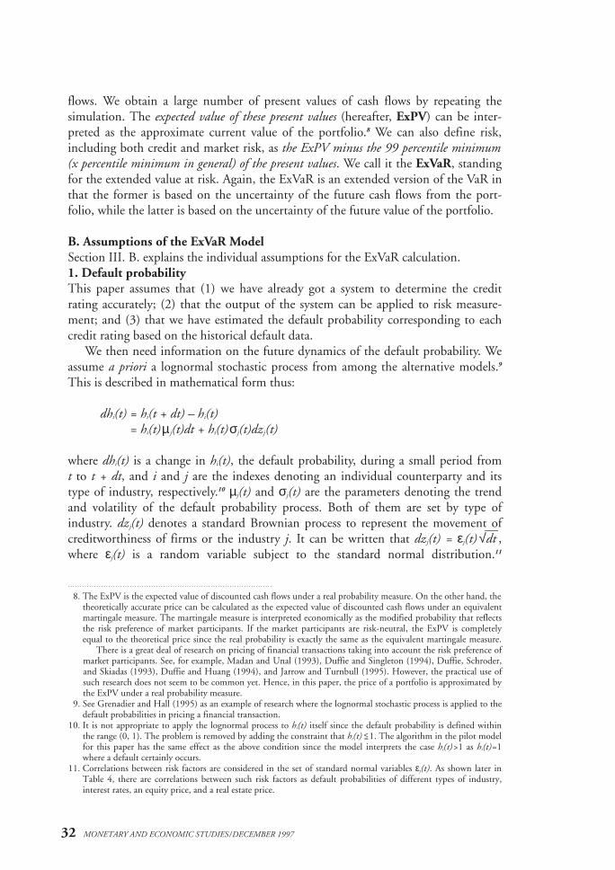
We then need information on the future dynamics of the default probability. Weassume a priori a lognormal stochastic process from among the alternative models.9
This is described in mathematical form thus:
dhi(t) = hi(t + dt) – hi(t) = hi(t)µ j(t)dt + hi(t)σj(t)dzj(t)
where dhi(t) is a change in hi(t), the default probability, during a small period from t to t + dt, and i and j are the indexes denoting an individual counterparty and itstype of industry, respectively.10 µj(t) and σj(t) are the parameters denoting the trendand volatility of the default probability process. Both of them are set by type ofindustry. dzj(t) denotes a standard Brownian process to represent the movement ofcreditworthiness of firms or the industry j. It can be written that dzj(t) = εj(t) √dt
—,
where εj(t) is a random variable subject to the standard normal distribution.11
32 MONETARY AND ECONOMIC STUDIES/DECEMBER 1997
8. The ExPV is the expected value of discounted cash flows under a real probability measure. On the other hand, thetheoretically accurate price can be calculated as the expected value of discounted cash flows under an equivalentmartingale measure. The martingale measure is interpreted economically as the modified probability that reflectsthe risk preference of market participants. If the market participants are risk-neutral, the ExPV is completelyequal to the theoretical price since the real probability is exactly the same as the equivalent martingale measure.
There is a great deal of research on pricing of financial transactions taking into account the risk preference ofmarket participants. See, for example, Madan and Unal (1993), Duffie and Singleton (1994), Duffie, Schroder,and Skiadas (1993), Duffie and Huang (1994), and Jarrow and Turnbull (1995). However, the practical use ofsuch research does not seem to be common yet. Hence, in this paper, the price of a portfolio is approximated bythe ExPV under a real probability measure.
9. See Grenadier and Hall (1995) as an example of research where the lognormal stochastic process is applied to thedefault probabilities in pricing a financial transaction.
10. It is not appropriate to apply the lognormal process to hi(t) itself since the default probability is defined withinthe range (0, 1). The problem is removed by adding the constraint that hi(t) =<1. The algorithm in the pilot modelfor this paper has the same effect as the above condition since the model interprets the case hi(t)>1 as hi(t)=1where a default certainly occurs.
11. Correlations between risk factors are considered in the set of standard normal variables εj(t). As shown later inTable 4, there are correlations between such risk factors as default probabilities of different types of industry,interest rates, an equity price, and a real estate price.

This model reflects the idea that grouping the homogeneous counterparties in termsof the default probability process can be achieved by classifying them on the basis ofthe type of industry. Therefore, parameter settings and random number generationare done by type of industry, not by counterparty, and the calculation burden ismarkedly reduced. It should be noted that only one attribute of counterparties—typeof industry—may be insufficient to grasp the characteristics of their default probabil-ity change. Other than the type of industry, such attributes as credit rating, region (orthe country), or the size of the counterparties can also be effective for grouping.Although we need detailed empirical study of the issue before implementing the riskmeasurement system, we focus a priori on the industry type factor in describing theExVaR framework. Empirical analysis is also required to estimate the parameters µj(t)and σj(t). In this paper, we estimate them from the historical data, assuming that thetrend is always zero and volatility is constant with regard to the time. (The result isshown in Table 4 later.) For more accurate and forward-looking analysis, we shouldmake adjustments for the effect of macroeconomic fluctuations due to the businesscycle. In our calculation, the time interval, dt, is set to one month and a period of upto five years is considered.2. Credit enhancement (collateral effect in particular)In Japan and other countries, a number of loans have some credit-enhancing features,typically a collateral or a guarantee. We should evaluate the effect appropriately since it has a large influence on both the value and the risk of the transaction. In this paper, we focus on the treatment of collateral—mainly real estate and equitycollateral—although many other forms of credit enhancement are actually available.
In collateral loans, a creditor is expected to collect the minimum amount of thefollowing three items in case of a default of a debtor (when the recovery rate on thesecured asset is 100 percent):
[1] fair value (replacement cost) of the transaction at the time of default;[2] fair value of the collateral (minus the amount of preemption of others, if any);
and[3] collateral limit (kyokudo-gaku).Thus, we need to model the future dynamics of collateral value in addition to that
of the market rates underlying the transaction. In this paper, we do not discuss howto construct the model but assume a priori a lognormal stochastic process for pricesof real estate and the equity of collateral. This assumption seems appropriate for theequities but may not hold good for real estate. Moreover, the dynamics of each realestate, or each equity, differ individually. However, we assume, for simplification, that all types of collateral have a uniform rate of return, which is equal to that of thebenchmark—the Land Price Indexes of Urban Districts (all urban districts, average),published by Japan Real Estate Institute, for real estate and the Nikkei 225 StockAverage for equities. In addition, we also posit a third collateral class, other collateral.In this paper, we assume the deposits are dominant in other collateral and set theprice volatility of this category to zero. 3. Recovery ratesThe treatment of recovery rates influences the estimation of credit risk as much asthat of the credit enhancement effect. Many approaches to this issue are possible,
33
A New Framework for Measuring the Credit Risk of a Portfolio

from a simple method of setting a specific constant as “the average recovery rate” or“the recovery rate of each asset class” to a more statistical method of modeling thefuture recovery rate with a stochastic process.
In our model, two kinds of recovery rates are to be input—the secured assetrecovery rate and the unsecured asset recovery rate. The former means theexpected rate of collected cash to the fair value of collateral in the defaulted securedasset, and the latter means the expected rate of collected cash to the pre-default fairvalue of the unsecured asset. The secured asset recovery rate is ideally equal to one,but it is actually less than one due to the existence of negotiation costs with subordi-nated collateral holders or the decrease of time value until completion to liquidatethe collateral. In this paper, we assume a priori that the rate is equal to 0.9. The un-secured asset recovery rate reflects the situation where some portion of the unsecuredasset could be recovered in some cases. In this paper, we conservatively set the rateequal to zero. 4. Interest rates12
Future yield curve movements are simulated by a combination of the Monte Carlomethod and a factor model in which three major vectors13 are adopted as factors fromamong the principal components of monthly yield curve data during the past eightyears. This approach has the advantage that it facilitates interpretation of change inthe yield curve. There are some alternative approaches, such as simulation with amultivariate normal distribution applied to the set of interest rates corresponding tospecific periods.5. Integration of credit and market risk (correlation between default probabili-
ties and market rates)Changes in the default probability of counterparties and changes in market rates,such as interest rates, are not in general independent of each other. For example, in arecession period, default probabilities tend to increase while interest rates tend todecrease, reflecting monetary expansion. Thus, there is a negative correlation betweenthe two variables.14 We take the correlations into account by jointly estimating the credit and market risks. In this paper, we calculate the correlation matrix of thedefault probabilities of each industry and the random factors corresponding to the three major principal components of yield curve movements, and use the matrixto simulate variables in the future.6. Time horizon of the risk evaluationWe set the risk evaluation period, during which the cash flow from a transaction isanalyzed and its uncertainty is the source of the risk, for each transaction in theportfolio. The concept of this period is similar to that of the so-called holdingperiod—typically one day—in the traditional VaR for market risk. In the ExVaRcalculation, however, the period is a time horizon of the risk evaluation, rather than
34 MONETARY AND ECONOMIC STUDIES/DECEMBER 1997
12. Although this paper deals with the interest rates in a single currency—Japanese yen—it is easy to extend theanalysis to multicurrency portfolios.
13. The three principal components of the yield curve movement can be interpreted, in turn, as (1) the parallel shift;(2) the change of the slope; and (3) the change of the curvature of the yield curve. Many empirical studies reportthat these three components can explain more than 99 percent of total yield curve movement.
14. See, for example, Duffee (1994, 1995), who reports an empirical study using the data in the United States.

the period during which a portfolio is held. Therefore, we call it the risk evaluationperiod in this paper.
We define the risk evaluation period of a transaction to be the estimated periodrequired to complete the liquidation of a transaction after deciding to do so. For example,one day would be acceptable as the period for highly liquid bonds. On the otherhand, the time to maturity would be appropriate as the period for loans whichcannot readily be liquidated. This definition is natural in terms of the meaning ofrisk.15 We should note again that the risk evaluation period is set according to trans-action, not portfolio. In chapters IV. and V., we set the period a priori to be the timeto maturity of each transaction for loans and swaps and one year for all debentures. 7. Diversification/concentration effectThe effect of investment diversification/concentration on credit risk is also impor-tant. In the ExVaR framework, the effect is automatically taken into account sincethe information on individual transactions are input and dealt with. We test theeffect in Section IV. B.
C. Specifications of the ExVaR ModelThe structure of our pilot model for calculating the ExVaR is shown in Figure 1. Theinformation input in five files is processed along the flow chart. A single simulationcorresponds to the procedures within the dotted line of Figure 1, outputting apresent value of cash flows from the portfolio given simulated market information. A histogram showing the distribution of the present values can be obtained byrepeating the simulation many times. After the calculation of the ExPV (expectedvalue of the present values), ExVaR can be derived as the ExPV minus the minimumpresent value with a 99 percentile confidence level, for example. Each file shown inFigure 1 is explained below.
[Input File 1]The file stores the data on the individual financial transactions. An example is shownin Table 1, including the information such as counterparty names (or indexes), trans-action categories (or indexes), principal, interest rates, time to maturity, collateralcategories (or indexes), collateral values, collateral limits, and preemption amounts.In the case of a plain interest rate swap (as opposed to a traditional loan), the princi-pal and the interest rate are interpreted as the notional amount and the fixed interestrate,16 respectively. In addition, the file also stores each transaction’s risk evaluationperiod, which is determined in accordance with the liquidity characteristics.
35
A New Framework for Measuring the Credit Risk of a Portfolio
15. Apart from the notion, adopted here, that the risk evaluation period is set individually according to the liquidityof each transaction, there is another way of thinking, which is that the unique period of risk evaluation is appliedto all transactions.
16. Where a spread is put on the floating rate side of the interest rate swap, the fixed-rate information to be input isthe notional fixed rate minus the spread.

36 MONETARY AND ECONOMIC STUDIES/DECEMBER 1997
Input File 1Transaction
data
Input File 2Counterparty
data
Input File 4Historical data
Yield curve generator
Principal componentanalysis
A simulation
Intermediate File 1Trend, volatility, and correlation
Intermediate File 4Future collateral value
Intermediate File 3Judgment of default realization
Pricing function for each transaction
Present value ofcash flows
Output File 2Histogram
Output File 3ExVaR
Intermediate File 6Present value of
cash flows
Output File 1Data set of
present values
Intermediate File 5Future yield curve
Input File 5Other parameters
Default probability by type of industry
Collateralasset prices
Market interestrates
Recoveryrates
Input File 3Default probability
by credit rating
Random number generator 1
Random number generator 2
Intermediate File 2Future default probability
of counterparties
Figure 1 Structure of the ExVaR Model

37
A New Framework for Measuring the Credit Risk of a Portfolio
Table 1 An Example of Input File 1
Transaction Counterparty Transaction Principal Interest rate Time to Risk Collateral Collateral Collateral Preemptioncode name category (¥ billions) (percent maturity evaluation category value limit amount
(index) (index*) per annum) (year) period (year) (index**) (¥ billions) (¥ billions) (¥ billions)
1 1 1 0.5 4.0 3.0 3.0 0 0 0 0
2 1 2 1.0 3.7 5.0 1.0 0 0 0 0
3 2 1 1.2 6.0 3.0 3.0 1 2.0 1.2 0.5
4 2 3 1.2 5.0 3.0 3.0 0 0 0 0
5 3 1 1.0 4.5 2.0 2.0 1 1.3 1.0 0
6 3 4 2.0 5.1 3.0 3.0 0 0 0 0
7 4 1 1.5 5.0 4.0 4.0 1 1.5 1.5 0
8 4 3 1.5 4.9 4.0 4.0 0 0 0 0
9 5 1 0.5 6.0 2.0 2.0 2 0.6 0.5 0
10 5 4 1.0 5.0 5.0 5.0 0 0 0 0
11 6 1 1.5 3.5 5.0 5.0 0 0 0 0
12 6 2 1.0 3.4 3.0 1.0 0 0 0 0
13 7 1 0.8 4.5 2.0 2.0 1 0.7 0.8 0
14 7 3 0.8 4.8 2.0 2.0 0 0 0 0
15 8 1 0.6 6.5 3.0 3.0 2 0.7 0.6 0
16 8 4 1.0 5.3 2.0 2.0 0 0 0 0
17 9 1 1.4 5.0 5.0 5.0 1 2.0 1.4 0.5
18 9 3 1.4 5.0 5.0 5.0 0 0 0 0
19 10 1 1.0 5.0 4.0 4.0 1 1.2 1.0 0
20 10 4 1.5 5.0 3.0 3.0 0 0 0 0. . . . . . . . . . .. . . . . . . . . . .. . . . . . . . . . .
*1 = Loan (no amortization), 2 = Corporate bond (fixed coupon), 3 = Interest swap (pay-fix, plain), 4 = Interest swap (receive-fix, plain)**0 = Non-collateral, 1 = Real estate collateral, 2 = Equity collateral, 3 = Other collateral (e.g., deposit)
[Input File 2]The file stores data on counterparties. An example is shown in Table 2, including thecounterparties’ credit ratings and attributes by which we classify firms into homoge-neous groups. In this paper, only the type of industry is used as an attribute.
Table 2 An Example of Input File 2
Counterparty CounterpartyCredit rating
Type of industry Size Regionindex name (index) (index) (index)
1 Firm XXX 3 1 — —
2 Firm YYY 6 1 — —
3 Firm ZZZ 4 2 — —
4 Firm ....... 5 3 — —
5 Firm ....... 6 3 — —
6 Firm ....... 2 3 — —
7 Firm ....... 4 4 — —
8 Firm ....... 7 6 — —
9 Firm ....... 5 6 — —
10 Firm ....... 5 8 — —

38 MONETARY AND ECONOMIC STUDIES/DECEMBER 1997
[Input File 3]The file stores estimated default probabilities corresponding to each credit rating. Anexample is shown in Table 3. One of the common approaches for the estimation is toanalyze the historical data of defaults by ratings and to derive the average default ratein each rating.
Table 3 An Example of Input File 3
Credit ratingAverage default rate(percent per annum)
1 0.01
2 0.1
3 0.5
4 1.0
5 2.0
6 3.0
7 4.0
8 5.0
9 10.0
10 30.0
[Input File 4]The file stores historical time-series data on the average default probability by type ofindustry, collateral prices (or the price indexes), and market interest rates. In thispaper, the average default probability is roughly estimated as the ratio of the suspen-sion of business transactions with banks (Federation of Bankers Associations ofJapan), by type of industry, divided by the estimated number of corporations foundin the Corporate Business Statistics Quarterly (Ministry of Finance of Japan).
[Input File 5]The file stores all the required parameters that are not included in Input Files 1 to 4. In the current model, only the secured and unsecured asset recovery rates are includedin the file. Additional information can be stored here if the model is modified.
[Intermediate File 1]The file stores estimated statistics, such as the trend, volatility, and correlation of the historical time-series data in Input File 4. An example is shown in Table 4. In deriving these, it is assumed that the default probabilities and collateral asset pricesare subject to a lognormal process while market interest rates are analyzed in accord-ance with a factor model with three principal components (PC) as the factors. Thethree principal components are shown in Figure 2.
In calculating the ExVaR of test portfolios in chapters IV. and V., the data inTable 4 are basically applied.

39
A New Framework for Measuring the Credit Risk of a Portfolio
Table 4 An Example of Intermediate File 1
TransportationConstruction Wholesaling Manufacturing and com- Real estate Services Retailing Others Land price Nikkei IR movement IR movement IR movement
munications
Def. prob. Def. prob. Def. prob. Def. prob. Def. prob. Def. prob. Def. prob. Def. prob. Movement Movement First PC Second PC Third PC
Trend — — — — — — — — 0.050 0.086 — — —
Standard deviation 0.386 0.312 0.323 0.442 0.498 0.386 0.332 0.550 0.039 0.211 — — —
TransportationCorrelations Construction Wholesaling Manufacturing and com- Real estate Services Retailing Others Land price Nikkei IR movement IR movement IR movement
munications
Construction 1.000 0.767 0.812 0.569 0.713 0.773 0.807 0.508 –0.048 –0.137 –0.271 –0.018 0.241
Wholesaling 0.767 1.000 0.669 0.588 0.597 0.743 0.694 0.533 –0.122 –0.242 –0.452 0.012 0.159
Manufacturing 0.812 0.669 1.000 0.603 0.758 0.684 0.764 0.382 –0.128 –0.283 –0.065 0.133 –0.036
Transportationand 0.569 0.588 0.603 1.000 0.572 0.547 0.509 0.396 –0.138 –0.175 –0.077 –0.284 0.062
communications
Real estate 0.713 0.597 0.758 0.572 1.000 0.625 0.708 0.388 0.019 –0.147 –0.247 0.006 0.044
Services 0.773 0.743 0.684 0.547 0.625 1.000 0.726 0.508 –0.045 –0.216 –0.305 –0.030 0.324
Retailing 0.807 0.694 0.764 0.509 0.708 0.726 1.000 0.490 –0.035 –0.189 –0.126 0.039 0.081
Others 0.508 0.533 0.382 0.396 0.388 0.508 0.490 1.000 –0.062 0.098 –0.416 –0.006 –0.054
Land price –0.048 –0.122 –0.128 –0.138 0.019 –0.045 –0.035 –0.062 1.000 0.251 –0.070 –0.025 0.512
Nikkei –0.137 –0.242 –0.283 –0.175 –0.147 –0.216 –0.189 0.098 0.251 1.000 –0.095 –0.185 0.188
IR First PC –0.271 –0.452 –0.065 –0.077 –0.247 –0.305 –0.126 –0.416 –0.070 –0.095 1.000 –0.152 –0.153
IR Second PC –0.018 0.012 0.133 –0.284 0.006 –0.030 0.039 –0.006 –0.025 –0.185 –0.152 1.000 0.065
IR Third PC 0.241 0.159 –0.036 0.062 0.044 0.324 0.081 –0.054 0.512 0.188 –0.153 0.065 1.000
1.4
1.2
1.0
0.8
0.6
0.4
0.2
0
–0.25.04.54.03.53.02.52.01.51.00.5
Percent
Time to maturity (years)
First PCSecond PCThird PC
Figure 2 Three Principal Components of Interest Rate Movements

40 MONETARY AND ECONOMIC STUDIES/DECEMBER 1997
[Intermediate Files 2, 4, 5 and Random Number Generator 1]Random Number Generator 1 outputs multivariate normal random numbers,17 ofwhich the correlation is given by the result in Intermediate File 1. They are appliedto the stochastic model of each variable to simulate its movement. For example, thecurrent default probability of a firm is given by Input Files 2 and 3. Starting from theinitial probability, its future path evolves in accordance with both the generatedrandom numbers and the stochastic process of the industry to which the firmbelongs. An example is shown in Table 5. With the same procedures, collateral assetprices and the yield curve are simulated from initial period into the future. Examplesare shown in Table 6 and Figure 3, respectively.
17. Multivariate normal random numbers are generated in the pilot model by multiplying the Cholesky matrix witha vector composed of the standard normal random numbers that are generated by applying the Box-Müllermethod to uniform random numbers. In general, Monte Carlo simulations can be more effective by using (1) low discrepancy sequences, such as Sobol or Faure, instead of uniform random numbers; and (2) variancereduction procedures, such as the antithetic variable method.
Counterparty (index) 1 month 2 months 3 months . . . . . . 58 months 59 months 60 months1 3.00 3.08 3.15 . . . . . . 4.62 4.51 4.552 2.00 1.88 1.75 . . . . . . 2.13 2.30 2.283 0.10 0.11 0.10 . . . . . . 0.15 0.17 0.17
. . . . . . . . . .
. . . . . . . . . .
98 0.50 0.52 0.51 . . . . . . 0.42 0.40 0.3899 5.00 5.12 5.30 . . . . . . 4.87 4.75 4.82
100 0.10 0.09 0.11 . . . . . . 0.10 0.11 0.12
Collateral asset 1 month 2 months 3 months . . . . . . 58 months 59 months 60 monthscategoriesLand Price Indexes 93.15 92.91 92.67 . . . . . . 95.12 95.24 95.37
Nikkei 225 Stock Average 19,723 19,688 19,756 . . . . . . 21,020 21,154 21,254
1
2
3
4
510
20Time of evaluation (months)
3040
5060
0.15
0.10
0.05In
tere
st r
ate
Term structure (years)
Figure 3 An Example of Intermediate File 5
Table 6 An Example of Intermediate File 4
Table 5 An Example of Intermediate File 2

41
A New Framework for Measuring the Credit Risk of a Portfolio
[Intermediate File 3 and Random Number Generator 2]In a simulation, after determining the default probability paths, we need to judgewhether the firm defaults or not. There is no direct relationship, but only an indirectrelationship, between default probability magnitude and the realization of default. Inother words, a default may be realized by a firm with a very small default probabilitywhile a default may not be realized by a firm with a very large default probability.
Random Number Generator 2 outputs uniform random numbers between 0 and1. These are compared with the future default probability of a firm month by month.Where the random number is less than the default probability, this is interpreted asthe realization of default in the month concerned. The result of judgment is stored inIntermediate File 3, of which an example is shown in Table 7.
Table 7 An Example of Intermediate File 3■ 0 = Non-Default, 1 = Default
Counterparty (index) 1 month 2 months 3 months . . . . . . 58 months 59 months 60 months1 0 0 0 . . . . . . 0 0 02 0 0 0 . . . . . . 0 0 03 0 0 0 . . . . . . 1 — —. . . . . . . . . .. . . . . . . . . .
98 0 0 0 . . . . . . 0 0 099 0 0 1 . . . . . . — — —
100 0 0 0 . . . . . . 0 0 0
[Intermediate File 6]In a simulation, the realized cash flows can be determined given (1) the default/non-default information in Intermediate File 3; (2) the collateral values inIntermediate File 4; and (3) the transactions’ payoff based on the market rates inIntermediate File 5. The cash flows are assumed to be reinvested in riskless assetsuntil a specific date (five years later, in this paper) and the value discounted back tothe present. The present value is stored in Intermediate File 6. An example is shownin Table 8.
Table 8 An Example of Simulated Cash Flows and Present Value
¥ billionsTransaction (code) 0.5 year 1.0 year 1.5 years . . . . . . 4.0 years 4.5 years 5.0 years1 (loan, non-default) 0.025 0.025 0.025 . . . . . . 0.025 0.025 1.0252 (swap, non-default) –0.002 –0.002 –0.001 . . . . . . 0.002 0.001 0.0023 (loan, default, secured) 0.030 0.030 0.927 . . . . . . 0.000 0.000 0.0004 (loan, default, unsecured) 0.030 0.030 0.000 . . . . . . 0.000 0.000 0.000
. . . . . . . . . .
. . . . . . . . . .
Total cash flow 3.057 3.041 2.968 . . . . . . 2.554 2.544 98.521
Total present value 106.733
[Output File 1]The present value of cash flows is calculated many times by repeating the simulation.
➡

42 MONETARY AND ECONOMIC STUDIES/DECEMBER 1997
The result in Intermediate File 6 is stored every time in Output File 1. In this paper,the number of simulations is set between 10,000 and 100,000.
[Output File 2]The file contains a histogram made from the data in Output File 1. Three examplesare shown below.
Figure 4 [1] shows the result of 100,000 simulations involving a portfoliocomposed of 100 loans. Figure 4 [2] shows the result of 10,000 simulations of thesame portfolio. Figure 4 [3] shows the result of 10,000 simulations of a portfoliocomposed of 100 interest rate swaps (plain pay-fix rate). These results have threeimplications, as follows:
[1] The histogram of 100,000 simulations has a very smooth shape.[2] The histogram of 10,000 simulations also has a shape smooth enough to
permit analysis of the risk amount.[3] The shapes of histograms are not necessarily symmetrical.
[2] 10,000 Simulations for a Loan Portfolio
Figure 4 An Example of a Histogram of the Present Value of Cash Flows [1] 100,000 Simulations for a Loan Portfolio
60 65 80 95
Present value (¥ billions)
85 120105 110 11590 1000
0.010
0.005
0.015
0.020
0.030
0.025
70 75
95 percentile ExVaR99 percentile ExVaR
16.523.0 ExPV
Pro
babi
lity
dens
ity
60 65 80 95
Pro
babi
lity
dens
ity
Present value (¥ billions)
85 120105 110 11590 1000
0.010
0.005
0.015
0.020
0.030
0.025
70 7595 percentile ExVaR
99 percentile ExVaR
16.4
22.5 ExPV

43
A New Framework for Measuring the Credit Risk of a Portfolio
[Output File 3]The file contains the ExPV, which is interpreted as the approximate value of theportfolio, and the ExVaR, which is calculated from the data in Output File 1. In thispaper, ExVaR is calculated with a 99 percentile and/or 95 percentile confidence level.Figure 4 [1], [2], and [3] shows the ExPV and the ExVaR of each portfolio.
IV. Calculation of the ExVaR for Test Portfolios
The ExVaR model is constructed so that it can be effective with regard to the follow-ing four points that cannot be omitted from a proper evaluation of credit risk.
[1] Integration of on-balance and off-balance sheet transactions, with the riskevaluation period set in accordance with each transaction’s liquidity.
[2] Effect of diversification/concentration in terms of counterparties and attrib-utes of counterparties.
[3] Integrated evaluation of credit and market risk.[4] Effect of collateral.In this chapter, we assume a number of hypothetical test portfolios, and calculate
and compare their ExPV and ExVaR to investigate how the above four points arereflected in the results. This analysis not only certifies the effectiveness of the ExVaRframework but also suggests that the above four features need to be taken intoaccount in whatever models one uses to evaluate credit risk.
Specifications of test portfolios used in chapters IV. and V. are shown in the list inthe Appendix. The number of simulations is usually 10,000, except in cases whichrequire more accuracy, where we use 100,000 simulations.
A. Integration of On-Balance and Off-Balance Sheet Transactions with the RiskEvaluation Period Set Based on the Transaction’s Liquidity
Six test portfolios (#1-1 to #1-6) are set out below and their risk amounts evaluated.The analysis, serving as a simple example of an ExVaR calculation, describes twoaspects: the integration of on-balance and off-balance sheet transactions, and thesetting of the risk evaluation period according to the liquidity of the transaction.
[3] 10,000 Simulations for a Swap Portfolio
–15 10
Pro
babi
lity
dens
ity
Present value (¥ billions)
0 3020 255 150
0.015
0.005
0.0200.0250.030
0.0400.035
–1095 percentile ExVaR
99 percentile ExVaR10.5
13.7 ExPV
–5
0.010

44 MONETARY AND ECONOMIC STUDIES/DECEMBER 1997
1. Integrated risk evaluation of on-balance and off-balance sheet transactionsFirst, we set up six test portfolios as follows. Each portfolio has one or two transac-tions with 100 counterparties. Conditions other than the type of transaction arebasically the same for all six portfolios so that the difference of risk amounts can beattributed to the difference in the different types of transaction. That is, everycounterparty belongs to the same industry (industry #2 here18) and has the samedefault probability (3 percent per annum, which corresponds to credit rating #6 inthe paper). Looking at the individual portfolio, the portfolio #1-1 is composed of100 loans, each of which is a transaction with each counterparty. Every loan has thesame conditions: the principal is ¥1 billion, the interest rate is 5 percent per annum(payable semiannually), the time to maturity is five years (and the risk evaluationperiod is accordingly five years), and there is no collateral set. Portfolio #1-2 iscomposed of 100 debentures, each of which is issued by each counterparty. Everydebenture has the same conditions: the principal is ¥1 billion (with no sinkingprovision), the coupon rate is 5 percent per annum (payable semiannually), the timeto maturity is five years (but the risk evaluation period is one year, reflecting theliquidity), and there is no collateral set. Portfolio #1-3 is composed of 100 plaininterest rate swaps (paying fixed rates), each of which is a transaction with eachcounterparty. Every swap has the same conditions: the notional amount is ¥1 billion,the fixed interest rate is 5 percent per annum (payable semiannually), the time tomaturity is five years (and the risk evaluation period is accordingly five years), andthere is no collateral set. Portfolios #1-4, #1-5, and #1-6 are composed of 100 loansand debentures, 100 loans and swaps, and 100 debentures and swaps, respectively,while the other conditions are the same as those in portfolios #1-1, #1-2, and #1-3.
The calculated ExVaR of these portfolios is shown in Table 9.
18. In Chapter III., eight types of industry are specified as an example of classification. In Chapter IV., types ofindustry are denoted by the index numbers, 1 to 8, for convenience of description.
Table 9 ExPV and ExVaR of Test Portfolios #1-1 to #1-6
PortfolioPortfolio composition ExPV 95 percentile ExVaR 99 percentile ExVaR
100 loans 100 debentures 100 swaps (¥ billions) (¥ billions) (¥ billions)#1-1 ✓ 93.0 16.4 22.5#1-2 ✓ 88.6 11.7 15.8#1-3 ✓ 5.3 10.5 13.7#1-4 ✓ ✓ 181.6 25.2 34.8#1-5 ✓ ✓ 98.0 23.1 30.0#1-6 ✓ ✓ 93.7 18.7 24.1
The first implication from the results is that the integrated evaluation is supposed tomeasure the risk of a portfolio, including both on-balance and off-balance sheettransactions, rather than sum up the risks of separate sub-portfolios. For example, the 99 percentile ExVaR of portfolio #1-5, which is composed of loans and swaps, is ¥30billion while the summed ExVaR of portfolios #1-1 and #1-3, which are composed ofloans and swaps, respectively, is ¥36.2 billion. It means that the latter ExVaR shows tooconservative a value, which is 20 percent more than the former ExVaR. There is the same tendency in a combination of loans and debentures or of debentures and swaps.

45
A New Framework for Measuring the Credit Risk of a Portfolio
2. The effect of risk evaluation periodThe second implication from the above results is that the ExVaR is largely influencedby the risk evaluation period. For example, the 99 percentile ExVaR of portfolios #1-1and #1-2 is ¥22.5 billion and ¥15.8 billion, respectively. This large difference iscaused solely by the difference in risk evaluation period: five years for all transactionsin #1-1 and one year for all transactions in #1-2. Although the direction of the differ-ence can be easily imagined without any calculation, the degree of difference can befound only after quantitative analysis. To set the risk evaluation period accurately isespecially important for liquid transactions, since some discretion is unavoidable indetermining the period of such transactions. Figure 5 shows the ExVaR of portfolio#1-2 against the risk evaluation period, which is moved from half a year to five yearsfor every transaction in it. This suggests that the increase in risk accompanied bylengthening the period is slower than in the √
—T effect19 for the traditional VaR.
19. It is known that the VaR for the market risk is proportional to the square root of the risk evaluation period (i.e.,the holding period) in the case of measuring the risk of the assets of which the price is linear to the risk factor.
20. For example, one may short the equity of a firm to hedge the default risk of a loan to the firm. Although thehedge can be effective to some degree, it is not more than a rough cross-hedge in that the appropriate hedge ratiois difficult to determine. One may also use credit derivatives to completely hedge the default risk of a loan.However, it seems that the market for credit derivatives has not yet become mature enough to be used flexibly.
Figure 5 ExVaR and the Risk Evaluation Period
Risk evaluation 95 percentile ExVaR 99 percentile ExVaRperiod (years) (¥ billions) (¥ billions)
0.5 8.4 11.21.0 11.7 15.81.5 13.4 18.32.0 14.5 20.12.5 15.5 21.93.0 15.8 22.43.5 16.0 22.54.0 16.1 22.64.5 16.3 22.45.0 16.4 22.5
ExV
aR (
¥ bi
llion
s)
25
20
15
10
5
05.04.54.03.53.02.52.01.51.00.5
Risk evaluation period (years)
99 percentile95 percentile
B. The Effect of Diversification/ConcentrationOne of the most important points in credit risk management is the measurement andcontrol of the effect of credit diversification/concentration. This reflects the fact thatthere are currently very few tools for directly hedging credit risk,20 while the marketrisk can be flexibly hedged by various transactions. Therefore, many people suggestthat one should diversify the credit portfolio to reduce the risk effectively. However,financial institutions also find some advantage in concentrating their credit port-folios. For example, it is efficient to investigate and monitor counterparties thatspecialize in a certain industry or geometric area. Such a trade-off is well known as the credit paradox. To optimize the risk profile of a portfolio with the trade-offconsidered, we need to measure the risk amount that properly reflects thediversification/concentration effect. In Section IV. B., we set up some test portfoliosand calculate their ExVaR for comparison in order to investigate whether the ExVaRframework satisfies this prerequisite.

46 MONETARY AND ECONOMIC STUDIES/DECEMBER 1997
It is convenient to classify the diversification/concentration effect into the follow-ing two elements:
[1] Diversification/concentration in terms of counterparties.[2] Diversification/concentration in terms of attributes (types of industry) of
counterparties.Element [1] is the effect that the risk of a portfolio composed of a large number
of small loans is less than that of a portfolio composed of a small number of largeloans even if the total credits of both are the same. On the other hand, element [2] isthe effect that the risk of a portfolio composed of loans to counterparties in a largenumber of industries is less than that of a portfolio composed of loans to counterpar-ties in a small number of industries when all the other conditions affecting the twoportfolios are the same.
We see the two effects in turn below, as well as the effect of the volatility ofdefault probabilities on the risk amount.1. Diversification/concentration in terms of counterpartiesThe three portfolios used here are composed of 100, 50, and 20 loans, respectively,each of which has a principal of ¥1 billion, ¥2 billion, and ¥5 billion, respectively,and is given to different counterparties with the same default probability in the sameindustry (#2). Looking at the results shown in Figure 6, we see that the ExVaRdecreases as the number of counterparties in a portfolio increases. This phenomenonreflects the effect of diversification/concentration in terms of counterparties.
Figure 6 Number of Counterparties (Diversification) and ExVaR
Portfolio Number of Principal ExPV 95 percentile ExVaR 99 percentile ExVaRcounterparties (¥ billions) (¥ billions) (¥ billions) (¥ billions)
#2-1 100 1.0 93.0 16.4 22.5#2-2 50 2.0 93.0 17.9 25.1#2-3 20 5.0 93.4 22.5 30.0
ExV
aR (
¥ bi
llion
s)
40
30
20
10
01005020
Number of counterparties
99 percentile95 percentile
2. Diversification/concentration in terms of attributes (types of industry) ofcounterparties
The eight portfolios used here are composed of 100 loans with a principal of ¥10billion, each of which is given to 100 counterparties, where the number of types of industry of counterparties is 1, 2, . . . 8 in the respective portfolios. Looking at

47
A New Framework for Measuring the Credit Risk of a Portfolio
the results shown in Figure 7, we see that the ExVaR decreases as the number of types of industry of counterparties in a portfolio increases. This reflects the effect of diversification/concentration in terms of type of industry of counterparties.
Figure 7 Number of Types of Industry (Diversification) and ExVaR
Number of Number of Principal of ExPV 95 percentile ExVaR 99 percentile ExVaRPortfolio types of counterparties in loan (¥ billions) (¥ billions) (¥ billions)industry an industry (¥ billions)#2-4 1 100 1.0 93.3 18.7 27.8#2-5 2 50 1.0 92.9 14.4 18.8#2-6 3 33, 34 1.0 92.7 13.1 17.6#2-7 4 25 1.0 92.8 12.9 16.9#2-8 5 20 1.0 92.9 12.9 16.4#2-9 6 16, 17 1.0 92.8 12.6 16.1#2-10 7 14, 15 1.0 92.7 12.4 15.8#2-11 8 12, 13 1.0 92.9 12.2 16.1
3. The effect of the volatility of default probabilities on riskWe compare the ExVaR using the historical volatility (HV) of default probabilitieswith the ExVaR using the doubled HV. Looking at the results shown in Table 10, we see that (1) the ExVaR increases as the volatility increases; and (2) the degree of increase is moderate when the portfolio is diversified in terms of type of industryof counterparties.
ExV
aR (
¥ bi
llion
s)
30
25
20
15
10
5
087654321
Number of types of industry
99 percentile95 percentile
Table 10 Volatility of Default Probabilities and ExVaR
Number of Number of Principal of 95 percentile ExVaR 99 percentile ExVaRPortfolio types counterparties loan (¥ billions) (¥ billions)
of industry in an industry (¥ billions) HV × 1 HV × 2 HV × 1 HV × 2#2-1 1 100 1.0 16.4 30.1 22.5 49.7#2-5 2 50 1.0 14.4 23.2 18.8 33.8#2-7 4 25 1.0 12.9 17.7 16.9 23.9#2-11 8 12, 13 1.0 12.2 14.7 16.1 19.5

48 MONETARY AND ECONOMIC STUDIES/DECEMBER 1997
C. Integration/Separation of Credit and Market Risk EvaluationAll the ExVaR outputs thus far include both credit risk (type I and II) and marketrisk. Such a treatment is desired for integrating the overall risk in a portfolio.However, there may be some demands for separate evaluation of credit risk and/ormarket risk. Thus, in this section, we calculate the risks separately for a loan portfolioand for a swap portfolio. To isolate credit risk, simulations are carried out on thehypothetical condition that the principal component vectors representing yield curvevolatility are all zero. To isolate market risk, simulations are executed on the hypo-thetical condition that the default probabilities of counterparties are all zero and thevolatilities of default probabilities are also zero. These conditions are summarized inTable 11. The results of the ExVaR calculation are shown in Figure 8.
Table 11 Risks and Risk Factors
Figure 8 Separate Calculation of Credit and Market Risks
Risk factorCredit risk
Market risk Integrated riskType I only
Default probability (DP) Yes Yes No YesVolatility of DP No Yes No YesYield curve (YC) Yes Yes Yes YesVolatility of YC No No Yes Yes
ExP
V, E
xVaR
(¥
billi
ons)
0
–5
–10
–15
–20
–25
–30
–35
–40
Market risk Type I only Credit risk Integrated risk
95 percentile ExVaR 99 percentile
ExVaR
ExPV
■ Long Portfolio (#3-1)
Transaction ExPV 95 percentile 99 percentile Portfolio category Risk factor (¥ billions) ExVaR ExVaR
(¥ billions) (¥ billions)Market risk 105.8 11.2 14.3
#3-1 LoanCredit risk 93.4 14.9 21.3Type I only 92.7 7.1 9.4
Integrated risk 93.0 16.4 22.5Market risk 5.8 11.2 14.3
#3-2 SwapCredit risk 5.4 0.4 0.6Type I only 5.4 0.3 0.4
Integrated risk 5.3 10.5 13.7

49
A New Framework for Measuring the Credit Risk of a Portfolio
In accordance with the definitions in Section III. A., each risk in a loan portfolioand a swap portfolio can be described by the above figure.
Looking first at the risk profile of the loan portfolio, we see a distinct differencebetween total credit risk (type I and type II) and type I credit risk alone. As shown inSection II. A., type I credit risk is caused by the incompleteness of diversification ofthe portfolio. In other words, an ideally diversified portfolio does not have such risk.Hence, the type I credit risk observed here results from the fact that the number oftransactions in a portfolio is finite (i.e., 100), and this is interpreted as concentrationrisk. On the other hand, type II credit risk is caused by the uncertainty of futuredefault probability changes, which are independent of the diversification/concentra-tion effect. Total credit risk is type I plus type II credit risk. The integrated risksimultaneously evaluates total credit risk and market risk, which is generally differentfrom the simple sum of the individually evaluated total of credit risk and market risk.
On the other hand, looking at the risk profile of a swap portfolio, whose transac-tions have the same notional amount as the principal of the above loan, we see thatthe credit risk is much smaller than that of the loan portfolio. This reflects the factthat the expected future value of a swap position is far smaller than its notionalamount. We also see that the integrated risk is slightly smaller than the individuallyevaluated interest rate risk. Although this feature is not common to every swap port-folio, such a case is probable. To understand the phenomenon intuitively, we canthink of the possibility that a certain interest rate path could raise a large loss nearmaturity in case of non-default, but the interest rate risk could not be realized whenthe transaction is closed before maturity due to the default of the counterparty.
D. The Effect of CollateralAll the portfolios we have discussed thus far are composed only of unsecured transac-tions. In this section, we investigate the effect of collateral on price (ExPV) and risk(ExVaR). To focus on the collateral effect, we only calculate credit risk in this section,excluding interest rate risk.
ExP
V, E
xVaR
(¥
billi
ons)
0
–2
–4
–6
–8
–10
–12
–14
–16
95 percentile ExVaR
ExPV99 percentile
ExVaR
Market risk Type I only Credit risk Integrated risk
■ Swap Portfolio (#3-2)

50 MONETARY AND ECONOMIC STUDIES/DECEMBER 1997
1. Risk evaluation by type of collateral assetWe consider real estate and equity as the collateral assets in this paper, assuming thatthey vary subject to lognormal stochastic processes with a correlation between them.We set up 10 test portfolios composed of 100 loans, each of which has either realestate collateral or equity collateral. The only difference between the portfolios is theratio of the two types of collateral loans. We calculate the ExPV and ExVaR of a port-folio composed only of real estate collateral loans, a portfolio composed only ofequity collateral loans, portfolios composed of both real estate collateral loans andequity collateral loans, and a portfolio composed only of unsecured loans. The resultsare shown in Figure 9.
Figure 9 Risk Amount by Type of Collateral Asset
Non-collateral Real estate Equity collateral ExPV 95 percentile 99 percentilePortfolio (number of loans) collateral (number of loans) (¥ billions) ExVaR ExVaR
(number of loans) (¥ billions) (¥ billions)#4-1 100 — — 93.0 14.9 21.3#4-2 — 0 100 103.7 4.6 7.9#4-3 — 20 80 103.7 3.9 6.7#4-4 — 30 70 103.8 3.6 6.1#4-5 — 50 50 103.8 3.0 4.9#4-6 — 70 30 103.9 2.5 3.9#4-7 — 80 20 103.9 2.4 3.6#4-8 — 90 10 104.0 2.2 3.2#4-9 — 95 5 104.0 2.1 3.1#4-10 — 100 0 104.0 2.1 3.0
0
ExV
aR (
¥ bi
llion
s)
20Composition of real estate collateral (percent)
40 10080600
21
345
876
95 percentile ExVaR99 percentile ExVaR
Looking at the results, we see that the ExPV of a portfolio composed of collateralloans is larger than that of a portfolio composed of non-collateral loans. This isnatural since the credit enhancement effect of collateral increases the value of loans(in other words, it decreases the credit risk premiums). We also see that the ExVaR ofa portfolio composed of collateral loans is much smaller than that of a portfoliocomposed of non-collateral loans and that the ExVaR of a portfolio composed of realestate collateral loans is smaller than that of a portfolio composed of equity collateralloans. The latter reflects the fact that the volatility of real estate is smaller than that of equities as shown in Table 4 before. In addition, we observe, in Figure 9, slightconvexity in the curve that represents the ExVaR against the ratio of the two types ofcollateral loans in a portfolio. This can be interpreted as the effect of diversificationin collateral assets.

51
A New Framework for Measuring the Credit Risk of a Portfolio
2. The effect of recovery ratesAll the risks have been calculated thus far with the unsecured and secured assetrecovery rates fixed at 0.0 and 0.9, respectively, for all transactions. In reality, theappropriate recovery rates depend on the features of individual transactions.Although a strict treatment that includes such a dependency may be desired for exactrisk measurement, the use of constant rates for similar transactions, as in this paper,seems sufficient for an approximate risk estimate. In this case, we need to know howsensitive the resulting risk is to changes in the recovery rate settings. Figure 10 showsthe sensitivity of the ExPV and ExVaR to the secured asset recovery rate. It suggests alarge influence of the recovery rate on the estimation. For example, 99 percentileExVaR increases by approximately 50 percent (from ¥3.1 billion to ¥4.8 billion) asthe recovery rate is lowered from 0.9 to 0.7.
Figure 10 Secured Asset Recovery Rate and ExVaR
Recovery rate ExPV 95 percentile ExVaR 99 percentile ExVaR(¥ billions) (¥ billions) (¥ billions)
1.0 51.4 2.0 2.90.9 50.6 2.2 3.10.8 50.6 2.7 3.80.7 49.5 3.4 4.80.6 49.0 4.0 5.60.5 48.4 4.6 6.50.4 47.9 5.3 7.50.3 47.4 6.0 8.50.2 46.9 6.8 9.60.1 46.5 7.6 10.6
1.0
ExV
aR (
¥ bi
llion
s)
0.80.9
Recovery rate
0.60.7 0.10.3 0.20.5 0.40
4
2
6
8
12
10 99 percentile ExVaR95 percentile ExVaR
V. Practical Applications
In Chapter IV., we confirmed the basic characteristics of the ExVaR by calculating itfor a number of portfolios under various conditions. In this chapter, we investigatethe applicability of the ExVaR for practical use in the risk management of financialinstitutions.
A. Scenario Analysis and Stress Test on Movement of Real Estate Prices In this section, we study, from a technical point of view, whether the deterioration ofJapanese financial institutions’ assets after the collapse of the “bubble” could have

52 MONETARY AND ECONOMIC STUDIES/DECEMBER 1997
been reduced if credit risk monitoring by such a measure as the ExVaR had prevailedbefore. The issue is also interpreted as a verification of the ExVaR’s ability to forecastthe degree of possible deterioration of future assets. For simplification, we focus onreal estate among the items influenced by the “bubble.” We analyze the influence ofthe decrease in real estate prices on the risk of loans with real estate collateral and onthe risk of loans to the real estate industry.
First, four hypothetical portfolios are set up as follows. Each of them is composedof 100 loans with a real estate collateral. The portfolios differ in two ways: (1) thetypes of industry of counterparties included are diversified or concentrated only inthe real estate industry; and (2) the current value of the collateral of each loan islower21 or higher than the principal of the loan. The details of the four portfolios areshown in the Appendix. Next, as shown in Table 12, five scenarios are assumed show-ing a stochastic process (i.e., trend and volatility) of the real estate collateral price andof the default probability for the real estate industry. The ExVaR with scenario #2, inwhich all the parameters are based on the historical data, corresponds to the commonapproach to evaluating risk by the use of the past information. On the other hand,the ExVaR with other scenarios (#1, #3, #4, and #5), which includes some subjectivefactors, is interpreted as so-called scenario analysis, or as a stress test if the hypothesisis extreme.
Figure 11 shows the ExPV and 99 percentile ExVaR (only the credit risk) for thefour portfolios under the five scenarios. In the bar diagram, the ExVaR is shown bythe length of the bar, of which the upper end and the lower end correspond to the
Portfolio Characteristic Scenario #1 Scenario #2 Scenario #3 Scenario #4 Scenario #5of portfolio ExPV ExVaR ExPV ExVaR ExPV ExVaR ExPV ExVaR ExPV ExVaR
#5-1 Concentrated; 102.1 3.2 100.6 5.2 97.3 11.4 97.3 16.8 96.0 19.2insufficient collateral
#5-2 Diversified; 102.1 3.1 100.5 5.1 97.2 11.3 97.1 15.3 96.0 17.2insufficient collateral
#5-3 Concentrated; collateral 103.0 1.9 103.0 1.9 101.7 8.0 101.6 11.1 101.0 12.9rule observed
#5-4 Diversified; collateral 103.0 1.9 103.0 1.9 101.7 8.0 101.6 10.2 101.1 11.5rule observed
21. Actually, it is said that, during the “bubble” period in Japan, some financial institutions made real estatecollateral loans of which the principal was larger than the value of the real estate collateral, expecting a futureincrease in collateral value.
Table 12 Scenarios to Be Analyzed
Figure 11 Results of the Scenario Analysis
Land price Default probability ofreal estate industry
Characteristics of scenarioTrend Volatility Trend Volatility(per annum) (per annum) (per annum) (per annum)
Scenario #1 0.20 0.04* — 0.50* Bull market in real estate (RE) pricesScenario #2 0.05* 0.04* — 0.50* Neutral market in RE pricesScenario #3 –0.10 0.20 — 0.50* Bear market in RE pricesScenario #4 –0.10 0.20 0.20 1.00 Bear market in RE prices; depression in RE industryScenario #5 –0.10 0.20 0.50 1.00 Bear market in RE prices; serious depression in RE industry
Note: The asterisk (*) indicates the value to be estimated from historical data.
¥ billions

53
A New Framework for Measuring the Credit Risk of a Portfolio
ExPV and the 99 percentile minimum present value, respectively. Looking at the resultfor scenario #2 first, the portfolios (#5-3 and #5-4) with the collateral rule observed22
have relatively small risk (¥1.9 billion), disregarding the factor of diversification/concentration. The portfolios (#5-1 and #5-2) with collateral of less value have relatively large risk (approximately ¥5 billion) in comparison with portfolios #5-3and #5-4, but the absolute level of risk can be recognized as not too large, since therisk is limited within about 5 percent of the ExPV.23 Such an analysis based only onhistorical data ends up with an optimistic result.
Next, the ExVaR is analyzed for the subjective scenarios (#1, #3, #4, and #5).Scenario #3 puts a negative trend on the process of the real estate price and sets thevolatility higher than in the past. With this scenario, the ExVaR of portfolios #5-1and #5-2 are almost double the ExVaR with scenario #2 and the ExVaR of portfolios#5-3 and #5-4 are almost four times the ExVaR with scenario #2. Such results exposethe weakness of loan management that depends excessively on real estate collateral.Moreover, scenarios #4 and #5 allow the default probability of the real estate industryto be higher, assuming a depression in the industry, in addition to the same decreasein real estate prices as with scenario #3. With these scenarios, the ExVaR outputs forall five portfolios are higher than those in any former scenario. On the absolute levelof risk, the ExVaR outputs are also evaluated as extremely high. For example, eventhe ExVaR outputs for portfolios #5-3 and #5-4, which have conservative collateral,are larger than 10 percent of the ExPV of the respective portfolios.
22. The collateral rule here is assumed to prescribe that the principal of a loan should not be more than the collateralvalue times the fixed multiplier, which is set at 0.8 in this paper.
23. The portfolio of which the ExVaR is about 5 percent of the value (ExPV) can be recognized as satisfactory interms of the risk/value ratio if we assume, for example, that the BIS capital adequacy requirement implies apotential loss of 8 percent of the asset value in a financial institution.
Scenario #1
ExP
V, E
xVaR
(¥
billi
ons)
#2 #3 #4 #570
75
80
85
90
110
105
100
95
Scenario #1 #2 #3 #4 #570
75
80
85
90
110
105
100
95
Scenario #1 #2 #3
Portfolio #5-1
#4 #570
75
80
85
90
110
105
100
95
Scenario #1 #2 #3 #4 #570
75
80
85
90
110
105
100
95
Portfolio #5-2
Portfolio #5-3 Portfolio #5-4
ExP
V, E
xVaR
(¥
billi
ons)
ExP
V, E
xVaR
(¥
billi
ons)
ExP
V, E
xVaR
(¥
billi
ons)
ExVaR
ExPVExPV
ExPVExPV
ExVaRExVaR
ExVaR

54 MONETARY AND ECONOMIC STUDIES/DECEMBER 1997
Looking just at the above results, it seems that the ExVaR which is mechanicallycalculated based on the upward-sloping real estate historical prices could hardly havegiven us any warning of the possible impact of the collapse of the “bubble.” Thistemporary implication results partly from the inappropriate assumption that the realestate price follows a lognormal stochastic process. The historical data in Figure 12show that the usual lognormal process does not fit the movement of the real estateindex sufficiently in two ways: (1) the price movement in reality has been verysmooth along the trend; and (2) the price experienced a structural change, that is, thesudden change of the trend at the collapse of the “bubble.” Hence, applying thelognormal process to real estate price data could lead to the underestimation of therisk of a portfolio that is sensitive to the real estate price, since the risk of structuralchange cannot be taken into account and the volatility of the price is estimated asrelatively small.24 To overcome the problem, it is necessary to describe the real estateprice movement more accurately by means of a model with a “bubble”-generatingmechanism in it. This issue remains to be resolved. It would be interesting to studywhether the improved model for real estate prices enables the ExVaR to forecastobjectively the risk of the “bubble” collapse even from the historical data alone. Theimportant implication from the above analysis is that, if one had intended to investi-gate the effect of a possible stress in the real estate market, one could have realized theimpact by use of the ExVaR. Generally speaking, since the ExVaR measures risk innormal situations, it is desirable to complement the ExVaR analysis with such tools asa stress test, as is the case with the traditional VaR for market risk.
Figure 12 Real Estate Price Index, Stock Price Index, and Their Rate of Return
0
20
40
60
80
120
100
1970 72 74 76 78 80 82 84 86 88 90 92 940
5,00010,00015,000
25,00020,000
40,000Yen
35,00030,000
1970 72 74 76 78 80 82 84 86 88 90 92 94
–0.10–0.05
00.05
0.150.20
0.10
0.25
1970 72 74 76 78 80 82 84 86 88 90 92 94–0.6
–0.4
–0.2
0
0.4
0.2
0.6
1970 72 74 76 78 80 82 84 86 88 90 92 94
■ Land Price Index of Urban Districts (All Urban Districts, Average)
■ Nikkei 225 Stock Average
■ Rate of Semiannual Change of the Land Price Index
■ Rate of Semiannual Change of Nikkei 225 Stock Average
24. The volatility of the real estate price (the Land Price Indexes of Urban Districts) is estimated to be 3.9 percent,which is much smaller than that of the stock price (Nikkei 225 Stock Average), which is estimated to be 21.1 percent.

55
A New Framework for Measuring the Credit Risk of a Portfolio
B. Theoretical Spread Required in a New TransactionIn this section, a procedure is shown for the theoretical setting of the interest ratestandard, which may be called “interest rate guideline” or “transfer rate,” for a new loan.The required risk premium is calculated in accordance with the marginal increase in theExVaR and is taken into account in determining the interest rate standard.
First, it should be noted again that credit risk is largely influenced by the so-calledportfolio effect, such as the diversification effect. Hence, the marginal effect of a newloan on the existing portfolio should be evaluated, instead of the independent effectof the single loan, in measuring the ExPV or the ExVaR.
Let us assume the case, as an example of the theoretical determination of theinterest rate standard, that a new loan is added to an existing portfolio (#6-1) com-posed of 99 identical loans, where a new loan has the same conditions except for thecounterparty’s credit rating and collateral. The issue is to determine the interest rate tobe set for the new loan. Since the initial cash outflow for the new loan is ¥1 billion, theprincipal, we should find the interest rate at which the loan marginally increases the value of the portfolio by exactly ¥1 billion. Figure 13 shows the solution, as therisk-unadjusted interest rate standard, calculating the ExPV in the range of 3 percent to10 percent interest rates and plotting them in diagrams. The resulting rates are effectiveonly on the assumption that the financial institution is risk-neutral.
Since the actual financial institution is risk-averse, however, the risk premiumshould be added to the risk-unadjusted interest rate standard. This paper considers anapproach for the determination of the risk premium as follows. It is assumed that thefinancial institution recognizes the risk of a portfolio by the ExVaR with the specificconfidence level that the financial institution thinks is optimal according to its own riskpreference. For example, the more risk-averse it is, the higher confidence level itintends to measure the ExVaR with. The financial institution needs additionalcapital, of which the amount is equal to the marginal increase in the ExVaR, for a newloan to maintain the soundness of its business. The cost of capital is generally moreexpensive than that of other liabilities. We adopt a method, from among alternatives,to estimate the cost of capital, which we define as the notional cost minus the risk-freerate, as the market risk premium multiplied by the equity beta of the financial institu-tion.25 The idea is based on the capital asset pricing model (CAPM). In this paper, weassume a priori that the market risk premium is 6.0 percent, the equity beta is 1.0, and,as a result, the cost of capital (i.e., the required rate of return on capital) is 6.0 percent.This means that the annual cost of maintaining capital sufficient for the risk is given as6.0 percent of the ExVaR. Hence, the required spread as a risk premium to a new loanis 6.0 percent of the marginal ExVaR divided by the principal of the loan. By addingthis spread to the risk-unadjusted interest rate standard, we calculate the risk-adjustedinterest rate standard, which is also shown in Figure 13. This can be interpreted as theminimum requirement for the interest rate of a new loan so that the loan’s expectedloss and risk are compensated with the interest income. In this sense, a financial insti-tution can substitute the interest rate standard for the traditional transfer ratebetween the ALM section and the branches.
25. See, for example, Copeland, Koller, and Murrin (1990) on the method of estimating the cost of capital.

56 MONETARY AND ECONOMIC STUDIES/DECEMBER 1997
Figure 13 An Example of Calculations of the Interest Rate Standard
Existing portfolio A new loan Marginal 99 percentile ExVaR Interest rate standard
increase (percent)Credit rating Interest rate of ExPV Marginal Cost of capital Risk- Risk-Contents (default Collateral (percent) (¥ billions) increase (¥ billions) unadjusted adjustedprobability) (¥ billions)
3 0.90 0.13 0.0084 0.95 0.13 0.0085 0.99 0.13 0.008
Rating: 4 None6 1.04 0.13 0.008
5.18 5.26(1 percent) 7 1.08 0.13 0.0088 1.13 0.13 0.0089 1.17 0.13 0.008
10 1.22 0.13 0.0083 0.83 0.17 0.0104 0.87 0.18 0.0115 0.91 0.19 0.011
Rating: 6 None6 0.95 0.21 0.012
7.13 7.27(3 percent) 7 0.99 0.23 0.0148 1.04 0.23 0.0149 1.08 0.23 0.014
#6-110 1.12 0.24 0.014
3 0.77 0.41 0.0244 0.81 0.43 0.0265 0.85 0.44 0.026
Rating: 8 None6 0.89 0.44 0.026
8.66 8.94(5 percent) 7 0.93 0.45 0.0278 0.97 0.46 0.0289 1.01 0.47 0.028
10 1.05 0.48 0.0293 0.94 0.17 0.0104 0.98 0.16 0.0105 1.03 0.16 0.010
Rating: 6 Real 6 1.07 0.15 0.0094.34 4.43(3 percent) estate 7 1.11 0.15 0.009
8 1.16 0.15 0.0099 1.20 0.15 0.009
10 1.24 0.14 0.009
99 loansto industry #2;credit rating: 6
(default probability3 percent);
interest rate:5 percent
0.7 0.8 0.9 1.0
Marginal increase of ExPV (¥ billions)
1.2 1.31.1
34567
1098
0.7 0.8 0.9 1.0
Marginal increase of ExPV (¥ billions)
1.2 1.31.1
34567
1098
0.7
Inte
rest
rate
(per
cent
)
0.8 0.9 1.0
Marginal increase of ExPV (¥ billions)
1.2 1.31.134567
1098 Risk-adjusted
Risk-unadjusted
0.7 0.8 0.9 1.0
Marginal increase of ExPV (¥ billions)
1.2 1.31.134567
1098
Risk-adjustedRisk-unadjusted
Risk-adjustedRisk-unadjusted
Risk-adjustedRisk-unadjusted
■ Rating 4, Non-Collateral
Inte
rest
rate
(per
cent
)In
tere
st ra
te (p
erce
nt)
Inte
rest
rate
(per
cent
)
■ Rating 6, Non-Collateral
■ Rating 8, Non-Collateral ■ Rating 6, Collateralized

57
A New Framework for Measuring the Credit Risk of a Portfolio
Figure 13 assumes an existing portfolio composed of 99 identical loans andconsiders the addition of a new loan to the portfolio. As a new loan, four types ofloan are set up that differ from each other in credit rating or the presence ofcollateral. Looking at the results, we see that the interest rate standard for the loanwith collateral is lower than that for the loan without collateral. We also find thedistinct characteristic that the worse the credit rating of a new loan, the higher theinterest rate standard for the loan. While these tendencies may be obvious withoutany calculation for most financial institutions, few financial institutions appear toanalyze the issue for their operation as quantitatively and logically as proposed here.We admit that real business is so complex that such a theory is not always effective.Still, we should emphasize the importance of using some logic as the basis forpractical operations.
C. Applicability of ExVaR to the Asset Allocation Strategy in FinancialInstitutions
Such an index as the ratio of the realized, or the expected, rate of return to the risk ofa portfolio can be effective for a financial institution in managing its capital alloca-tion strategy. A typical example of such an index is the so-called risk-adjusted returnon capital (RAROC). If a universal bank, whose business ranges from retail bankingto investment banking, adopts this type of performance index, it needs to evaluatethe risk of different types of business on the same scale. For this purpose, the ExVaRcan function effectively, since its coverage of type of risk is broader—including creditrisk (type I and II) and market risk—than the traditional VaR, which is only formarket risk. For example, the ExVaR can provide meaningful information for afinancial institution to pursue an optimal business structure by comparing the risk-adjusted performance of retail banking with that of investment banking.
This performance index, which is applicable to different types of risk on the samescale, not only realizes the mutual comparison of these risks but also accuratelymeasures the total risk held in a financial institution. This enables the managementto evaluate clearly the soundness of the business and to take up a business opportu-nity effectively (in other words, appropriate risk taking). Moreover, improvement ofdisclosure is also expected from the standpoint of equity holders and investors.
VI. Conclusion
This paper proposed a new framework, which we call the ExVaR, for the integratedevaluation of both credit and market risk. Through the calculation of the risk ofhypothetical test portfolios, basic characteristics of the ExVaR were shown and itsapplicability was discussed.
In the conclusion, the results of this paper and the remaining issues are summarized.
A. Results of the Paper[1] The ExVaR evaluates both the credit and market risks of a portfolio on the same
scale, taking into account the effect of the liquidity of individual transactions in

58 MONETARY AND ECONOMIC STUDIES/DECEMBER 1997
the portfolio. As a result, the applicability of the ExVaR is broader than that ofthe traditional VaR.
[2] The ExVaR quantitatively reflects the effects of diversification/concentration andcollateral, both of which are unavoidable issues in the measurement of credit risk.
[3] The framework of the ExVaR can generally be applied to any type of financialtransaction, including derivative products.
[4] The limits of the ExVaR are discussed and the need for scenario analyses or stresstests is suggested.
B. Remaining Issues[1] Implementation of the ExVaR to a real large-sized portfolio held by a financial
institution should be realized. There are such issues as the effective sampling orgrouping of transactions, which substitutes for the input of the data for individualtransactions, and enables computation with less of a burden than the normalMonte Carlo simulation.
[2] The default probability movement model should be improved. For example,factor analysis with macroeconomic variables or a model including laggedvariables, such as ARIMA, could modify the simple mechanism of the lognormalprocess assumed in the paper.
[3] The effective attributes by which to define homogeneous firms with respect todefault probability movements should be studied empirically and theoretically.
[4] The real estate price movement model should be improved over and above thesimple lognormal process assumed in the paper.
[5] Individual issues such as the effect of guarantees, the treatment of subordinatedassets, and the estimation of recovery rates should be tackled.
[6] The method of pricing defaultable assets should be improved by implementingsome theoretical pricing models, rather than by an approximation with theexpected value of discounted future cash flows from the asset.
The ExVaR is a flexible and comprehensive framework for risk measurement.This means that one needs to investigate carefully how to place the individual build-ing blocks of the model for implementation. On the other hand, there is no singleoptimal method of measuring the risk that is applicable to every case, since themethod should be different as the purposes of measurement or the managementstrategy of the institution differ. Hence, it is important to interpret the concept of theExVaR as a framework and to make settings that are appropriate to the situation.

59
A New Framework for Measuring the Credit Risk of a Portfolio
Appendix: List of Test Portfolios Used for the ExVaR Calculation
IV. A. Integration of On-Balance and Off-Balance Sheet Transactions with the Risk Evaluation Period Set Based on the Transaction’s Liquidity
Portfolio #1-1
Number of counterparties Default Principal Interest Time to Holding CollateralTransaction probability (¥ billions) (percent) maturity period Ind. #I II III IV V VI VII VIII (percent) (years) (years) Value Limit Preempt.
Loan 100 100 3 1.0 5 5 5 None
Portfolio #1-2
Number of counterparties Default Principal Interest Time to Holding CollateralTransaction probability (¥ billions) (percent) maturity period Ind. #I II III IV V VI VII VIII (percent) (years) (years) Value Limit Preempt.
Debenture 100 100 3 1.0 5 5 1 None
Portfolio #1-3
Number of counterparties Default Principal Interest Time to Holding CollateralTransaction probability (¥ billions) (percent) maturity period Ind. #I II III IV V VI VII VIII (percent) (years) (years) Value Limit Preempt.
Swap (pay-fix) 100 100 3 1.0 5 5 5 None
Portfolio #1-4
Number of counterparties Default Principal Interest Time to Holding CollateralTransaction probability (¥ billions) (percent) maturity period Ind. #I II III IV V VI VII VIII (percent) (years) (years) Value Limit Preempt.
Loan 100 100 3 1.0 5 5 5 NoneDebenture 100 100 3 1.0 5 5 1 None
Portfolio #1-5
Number of counterparties Default Principal Interest Time to Holding CollateralTransaction probability (¥ billions) (percent) maturity period Ind. #I II III IV V VI VII VIII (percent) (years) (years) Value Limit Preempt.
Loan 100 100 3 1.0 5 5 5 NoneSwap (pay-fix) 100 100 3 1.0 5 5 5 None
Portfolio #1-6
Number of counterparties Default Principal Interest Time to Holding CollateralTransaction probability (¥ billions) (percent) maturity period Ind. #I II III IV V VI VII VIII (percent) (years) (years) Value Limit Preempt.
Debenture 100 100 3 1.0 5 5 1 NoneSwap (pay-fix) 100 100 3 1.0 5 5 5 None
IV. B. The Effect of Diversification/Concentration
Portfolio #2-1
Number of counterparties Default Principal Interest Time to Holding CollateralTransaction probability (¥ billions) (percent) maturity period Type I II III IV V VI VII VIII (percent) (years) (years) Value Limit Preempt.
Loan 100 100 3 1.0 5 5 5 None
Portfolio #2-2
Number of counterparties Default Principal Interest Time to Holding CollateralTransaction probability (¥ billions) (percent) maturity period Type I II III IV V VI VII VIII (percent) (years) (years) Value Limit Preempt.
Loan 50 50 3 2.0 5 5 5 None
Portfolio #2-3
Number of counterparties Default Principal Interest Time to Holding CollateralTransaction probability (¥ billions) (percent) maturity period Type I II III IV V VI VII VIII (percent) (years) (years) Value Limit Preempt.
Loan 20 20 3 5.0 5 5 5 None
Portfolio #2-4
Number of counterparties Default Principal Interest Time to Holding CollateralTransaction probability (¥ billions) (percent) maturity period Type I II III IV V VI VII VIII (percent) (years) (years) Value Limit Preempt.
Loan 100 100 3 1.0 5 5 5 None
Portfolio #2-5
Number of counterparties Default Principal Interest Time to Holding CollateralTransaction probability (¥ billions) (percent) maturity period Type I II III IV V VI VII VIII (percent) (years) (years) Value Limit Preempt.
Loan 100 50 50 3 1.0 5 5 5 None
Portfolio #2-6
Number of counterparties Default Principal Interest Time to Holding CollateralTransaction probability (¥ billions) (percent) maturity period Type I II III IV V VI VII VIII (percent) (years) (years) Value Limit Preempt.
Loan 100 33 33 34 3 1.0 5 5 5 None
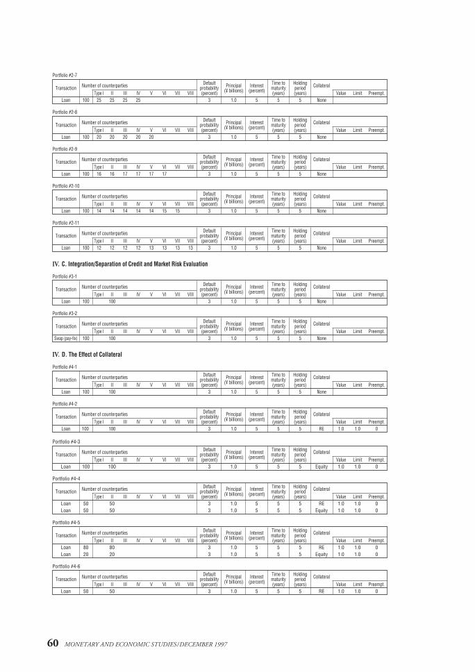
60 MONETARY AND ECONOMIC STUDIES/DECEMBER 1997
Portfolio #2-7
Number of counterparties Default Principal Interest Time to Holding CollateralTransaction probability (¥ billions) (percent) maturity period Type I II III IV V VI VII VIII (percent) (years) (years) Value Limit Preempt.
Loan 100 25 25 25 25 3 1.0 5 5 5 None
Portfolio #2-8
Number of counterparties Default Principal Interest Time to Holding CollateralTransaction probability (¥ billions) (percent) maturity period Type I II III IV V VI VII VIII (percent) (years) (years) Value Limit Preempt.
Loan 100 20 20 20 20 20 3 1.0 5 5 5 None
Portfolio #2-9
Number of counterparties Default Principal Interest Time to Holding CollateralTransaction probability (¥ billions) (percent) maturity period Type I II III IV V VI VII VIII (percent) (years) (years) Value Limit Preempt.
Loan 100 16 16 17 17 17 17 3 1.0 5 5 5 None
Portfolio #2-10
Number of counterparties Default Principal Interest Time to Holding CollateralTransaction probability (¥ billions) (percent) maturity period Type I II III IV V VI VII VIII (percent) (years) (years) Value Limit Preempt.
Loan 100 14 14 14 14 14 15 15 3 1.0 5 5 5 None
Portfolio #2-11
Number of counterparties Default Principal Interest Time to Holding CollateralTransaction probability (¥ billions) (percent) maturity period Type I II III IV V VI VII VIII (percent) (years) (years) Value Limit Preempt.
Loan 100 12 12 12 12 13 13 13 13 3 1.0 5 5 5 None
IV. C. Integration/Separation of Credit and Market Risk Evaluation
Portfolio #3-1
Number of counterparties Default Principal Interest Time to Holding CollateralTransaction probability (¥ billions) (percent) maturity period Type I II III IV V VI VII VIII (percent) (years) (years) Value Limit Preempt.
Loan 100 100 3 1.0 5 5 5 None
Portfolio #3-2
Number of counterparties Default Principal Interest Time to Holding CollateralTransaction probability (¥ billions) (percent) maturity period Type I II III IV V VI VII VIII (percent) (years) (years) Value Limit Preempt.
Swap (pay-fix) 100 100 3 1.0 5 5 5 None
IV. D. The Effect of Collateral
Portfolio #4-1
Number of counterparties Default Principal Interest Time to Holding CollateralTransaction probability (¥ billions) (percent) maturity period Type I II III IV V VI VII VIII (percent) (years) (years) Value Limit Preempt.
Loan 100 100 3 1.0 5 5 5 None
Portfolio #4-2
Number of counterparties Default Principal Interest Time to Holding CollateralTransaction probability (¥ billions) (percent) maturity period Type I II III IV V VI VII VIII (percent) (years) (years) Value Limit Preempt.
Loan 100 100 3 1.0 5 5 5 RE 1.0 1.0 0
Portfolio #4-3
Number of counterparties Default Principal Interest Time to Holding CollateralTransaction probability (¥ billions) (percent) maturity period Type I II III IV V VI VII VIII (percent) (years) (years) Value Limit Preempt.
Loan 100 100 3 1.0 5 5 5 Equity 1.0 1.0 0
Portfolio #4-4
Number of counterparties Default Principal Interest Time to Holding CollateralTransaction probability (¥ billions) (percent) maturity period Type I II III IV V VI VII VIII (percent) (years) (years) Value Limit Preempt.
Loan 50 50 3 1.0 5 5 5 RE 1.0 1.0 0Loan 50 50 3 1.0 5 5 5 Equity 1.0 1.0 0
Portfolio #4-5
Number of counterparties Default Principal Interest Time to Holding CollateralTransaction probability (¥ billions) (percent) maturity period Type I II III IV V VI VII VIII (percent) (years) (years) Value Limit Preempt.
Loan 80 80 3 1.0 5 5 5 RE 1.0 1.0 0Loan 20 20 3 1.0 5 5 5 Equity 1.0 1.0 0
Portfolio #4-6
Number of counterparties Default Principal Interest Time to Holding CollateralTransaction probability (¥ billions) (percent) maturity period Type I II III IV V VI VII VIII (percent) (years) (years) Value Limit Preempt.
Loan 50 50 3 1.0 5 5 5 RE 1.0 1.0 0
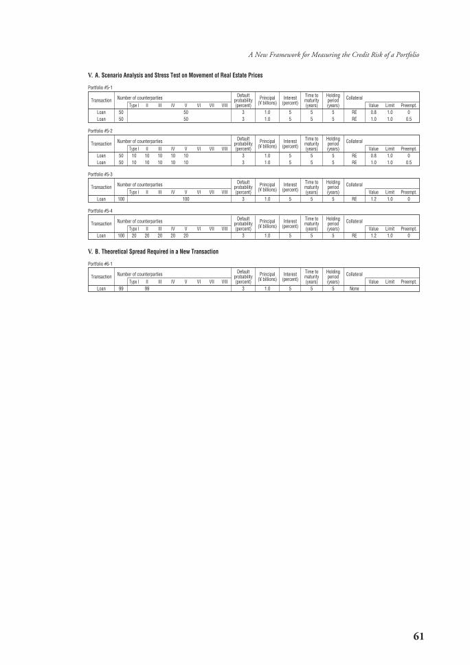
61
A New Framework for Measuring the Credit Risk of a Portfolio
V. A. Scenario Analysis and Stress Test on Movement of Real Estate Prices
Portfolio #5-1
Number of counterparties Default Principal Interest Time to Holding CollateralTransaction probability (¥ billions) (percent) maturity period Type I II III IV V VI VII VIII (percent) (years) (years) Value Limit Preempt.
Loan 50 50 3 1.0 5 5 5 RE 0.8 1.0 0Loan 50 50 3 1.0 5 5 5 RE 1.0 1.0 0.5
Portfolio #5-2
Number of counterparties Default Principal Interest Time to Holding CollateralTransaction probability (¥ billions) (percent) maturity period Type I II III IV V VI VII VIII (percent) (years) (years) Value Limit Preempt.
Loan 50 10 10 10 10 10 3 1.0 5 5 5 RE 0.8 1.0 0Loan 50 10 10 10 10 10 3 1.0 5 5 5 RE 1.0 1.0 0.5
Portfolio #5-3
Number of counterparties Default Principal Interest Time to Holding CollateralTransaction probability (¥ billions) (percent) maturity period Type I II III IV V VI VII VIII (percent) (years) (years) Value Limit Preempt.
Loan 100 100 3 1.0 5 5 5 RE 1.2 1.0 0
Portfolio #5-4
Number of counterparties Default Principal Interest Time to Holding CollateralTransaction probability (¥ billions) (percent) maturity period Type I II III IV V VI VII VIII (percent) (years) (years) Value Limit Preempt.
Loan 100 20 20 20 20 20 3 1.0 5 5 5 RE 1.2 1.0 0
V. B. Theoretical Spread Required in a New Transaction
Portfolio #6-1
Number of counterparties Default Principal Interest Time to Holding CollateralTransaction probability (¥ billions) (percent) maturity period Type I II III IV V VI VII VIII (percent) (years) (years) Value Limit Preempt.
Loan 99 99 3 1.0 5 5 5 None

62 MONETARY AND ECONOMIC STUDIES/DECEMBER 1997
Altman, E. I., Corporate Bankruptcy in America, D. C. Heath and Company, 1971.———, Corporate Financial Distress: A Complete Guide to Predicting, Avoiding, and Dealing with
Bankruptcy, New York: John Wiley & Sons, 1983.Backman, A. C., et al., Derivative Credit Risk: Advances in Measurement and Management, London: Risk
Publications, 1995.Boyes, W. J., D. L. Hoffman, and S. A. Low, “An Econometric Analysis of the Bank Credit Scoring
Problem,” Journal of Econometrics, 40 (1), 1989, pp. 3–14.Copeland, T., T. Koller, and J. Murrin, Valuation: Measuring and Managing the Value of Companies,
New York: John Wiley & Sons, 1990.Duffee, G. R., “On Measuring Credit Risks of Derivative Instruments,” Finance and Economic
Discussion Series 94-27, Federal Reserve Board, 1994.———, “The Variation of Default Risk with Treasury Yields,” mimeo, Federal Reserve Board, 1995.Duffie, D., M. Schroder, and C. Skiadas, “Two Models of Price Dependence on the Timing of
Resolution of Uncertainty,” Working Paper No. 177, Kellogg Graduate School ofManagement, Northwestern University, 1993.
———, and K. Singleton, “Econometric Modeling of Term Structure of Defaultable Bonds,” workingpaper, Graduate School of Business, Stanford University, 1994.
———, and M. Huang, “Swap Rates and Credit Quality,” working paper, Graduate School ofBusiness, Stanford University, 1994.
Goto, J., Kigyo Tohsan to Kaikei Joho (Corporate Bankruptcy and Accounting Information), Tokyo:Chikura Shobo, 1989 (in Japanese).
Grenadier, S. R., and B. J. Hall, “Risk-Based Capital Standards and the Riskiness of Bank Portfolios:Credit and Factor Risks,” NBER Working Paper No. 5178, 1995.
Jarrow, R. A., and S. M. Turnbull, “Pricing Derivatives on Financial Securities Subject to Credit Risk,”Journal of Finance, 50, 1995, pp. 53–85.
Johnsen, T., and R. W. Melicher, “Predicting Corporate Bankruptcy and Financial Distress:Information Value Added by Multinomial Logit Models,” Journal of Economics and Business, 46,1994, pp. 269–286.
Madan, D. B., and H. Unal, “Pricing the Risks of Default,” working paper, College of Business,University of Maryland, 1993.
Merton, R. C., “On the Pricing of Corporate Debt: The Risk Structure of Interest Rates,” Journal ofFinance, 29, 1974, pp. 449–470.
Mori, A., M. Ohsawa, and T. Shimizu, “Calculation of Value at Risk and Risk/Return Simulation,”IMES Discussion Paper Series 96-E-8, Bank of Japan, 1996.
Nishida, S., ALM Shuho no Shin-Tenkai (New Developments in ALM Methodology), Tokyo: NihonKeizai Shimbun-sha, 1995 (in Japanese).
Sekino, K., and K. Sugimoto, Risuku Manejimento (Risk Management), Tokyo: Kinyu Zaisei JijoKenkyu-kai, 1993 (in Japanese).
Wu, C., and C. Yu, “Risk Aversion and the Yield of Corporate Debt,” Journal of Banking and Finance,20, 1996, pp. 267–281.
References