A new hyperbolic GARCH model

Muyi Li, Wai Keung Li and Guodong Li

Xiamen University and University of Hong Kong

April 16, 2014

Abstract

There are two commonly used hyperbolic GARCH processes, the FIGARCH

and HYGARCH processes, in modeling the long-range dependence in volatility.

However, the FIGARCH process always has infinite variance, and the HYGARCH

model has a more complicated form. This paper builds a simple bridge between

a common GARCH model and an integrated GARCH model, and hence a new

hyperbolic GARCH model along the lines of FIGARCH models. The new model

remedies the drawback of FIGARCH processes by allowing the existence of finite

variance as in HYGARCH models, while it has a form nearly as simple as the

FIGARCH model. Two inference tools, including the Gaussian QMLE and a

portmanteau test for the adequacy of the fitted model, are derived, and an easily

implemented test for hyperbolic memory is also constructed. Their finite sample

performances are evaluated by simulation experiments, and an empirical example

gives further support to our new model.

JEL Classification: C15; C22

Keywords: ARCH(∞), Hyperbolic GARCH, Long-range dependence, QMLE.

1

1 Introduction

Ding et al. (1993) and Dacorogna et al. (1993) first observed long-range dependence in

squared returns, as well as other power transformed absolute returns, of asset prices;

see also Ding and Granger (1996). Due to the popularity of ARCH-type models (Engle,

1982; Bollerslev, 1986), it is convenient to discuss such type of long memory feature un-

der the framework of ARCH(∞) models (Robinson, 1991). We may follow the classical

approach and define that a sequence of returns yt exhibits long memory in volatility

if the autocovariance function cov(y2t , y2t−k) is not absolutely summable. However, under

the condition of E(y4t ) < ∞, ARCH(∞) processes always have absolutely summable

autocovariances; see Giraitis et al. (2000), Giraitis and Surgailis (2002) and Zaffaroni

(2004). In order to measure the memory of an ARCH(∞) process more precisely, David-

son (2004) suggested the concept of hyperbolic memory instead of long memory, and the

process is said to have hyperbolic (geometric) memory if its coefficients decay hyperbol-

ically (geometrically). Note that the autocovariance function cov(y2t , y2t−k) also decays

hyperbolically (geometrically) for a hyperbolic (geometric) memory ARCH(∞) process.

Consider the GARCH model,

yt = εt√ht, ht = γ+

Q∑i=1

αiy2t−i+

P∑j=1

βjht−j or ht =γ

β(1)+

1− δ∗(B)

β(B)

y2t , (1)

where εt are identically and independently distributed (i.i.d.) with mean zero and

variance one, γ > 0, αi ≥ 0, βj ≥ 0, B is the back shift operator, β(x) = 1−∑P

j=1 βjxj,

α(x) =∑Q

i=1 αixi and δ∗(x) = β(x)−α(x); see Bollerslev (1986). It is obvious that model

(1) has geometric memory. This paper will focus on the hyperbolic memory ARCH(∞)

models originating from the GARCH model (1), and calls them hyperbolic GARCH

models for simplicity.

For the integrated GARCH model, its conditional variance (1) has the form

ht =γ

β(1)+

1− δF (B)

β(B)(1−B)

y2t ,

where δ∗(x) = δF (x)(1 − x) since∑Q

i=1 αi +∑P

j=1 βj = 1. By replacing (1 − B) with

(1−B)d on the right hand side of the above equation, Baillie et al. (1996) proposed the

fractionally integrated GARCH (FIGARCH) model, where 0 < d < 1 and (1 − B)d =

2

1−∑∞

j=1 πjBj with

πj =dΓ(j − d)

Γ(1− d)Γ(j + 1)= O(j−1−d). (2)

This is the first hyperbolic GARCH model in the literature. However, as for the inte-

grated GARCH process, the FIGARCH process always has infinite variance, and this

limits its applications. To overcome this drawback, Davidson (2004) proposed a hyper-

bolic GARCH (HYGARCH) model,

yt = εt√ht, ht =

γ

β(1)+

1− δH(B)

β(B)[1− ϕ+ ϕ(1−B)d]

y2t , (3)

where ϕ > 0. This model will reduce to the FIGARCH model if ϕ = 1, and the variance

of yt is finite when 1− (1−ϕ)δH(1)/β(1) < 1. Note that the polynomial δ∗(x) in (1) has

a unique root on R+, say 1/ϕ, and in terms of ϕ the conditional variance of the GARCH

model has the form

ht =γ

β(1)+

1− δH(B)

β(B)(1− ϕB)

y2t =

γ

β(1)+

1− δH(B)

β(B)[1− ϕ+ ϕ(1−B)]

y2t ,

i.e. we can arrive at the HYGARCH model after replacing (1−B) with (1−B)d in the

above equation; see Li et al. (2011). Note that coefficients πjs in (2) have more persistence

as d decreases, and the memory of (1 − B)d is continuous at d = 1 (Davidson, 2004).

By letting 0 < d ≤ 1, the HYGARCH model can then be extended to encompass the

common GARCHmodel with geometric memory (Li et al., 2011). Robinson and Zaffaroni

(2006) also considered a hyperbolic GARCH model, however, it has not attracted much

attention so far.

For an ARCH(∞) model, it is necessary to restrict all its coefficients to be non-

negative such that the conditional variance ht ≥ 0 with probability one. Non-negativity

conditions for FIGARCH and HYGARCH models were discussed respectively by Conrad

and Haag (2006) and Conrad (2010). It is obvious that the HYGARCH model has more

complicated restrictions than those of the FIGARCH model. Consider the conditional

variance of the HYGARCH process in (3). It can be rewritten as ht = (1− ϕ)h1t + ϕh2t,

where

h1t =γ

β(1)+

1− δH(B)

β(B)

y2t and h2t =

γ

β(1)+

1− δH(B)

β(B)(1−B)d

y2t ; (4)

3

see Li et al. (2011) and Li et al. (2013). It can be seen that the FIGARCH component

h2t already has the multiplicative form of a geometric decaying pattern δH(B)/β(B) and

a hyperbolic decaying pattern (1−B)d, i.e. the conditional variance of the HYGARCH

process may have an unnecessarily complicated form. Moreover, the parameters d and ϕ

are both related to the memory of a HYGARCH process. This motivates us to consider

a new decomposition of the GARCH model with a simpler structure, and it then leads to

a new hyperbolic GARCH model in section 2. The proposed model allows the existence

of finite variance as in HYGARCH models, while it has a form nearly as simple as

FIGARCH models.

Section 3 derives the Gaussian quasi-maximum likelihood estimation (QMLE) for

the new model and a portmanteau test for the adequacy of the fitted model. An easily

implemented test for the hyperbolic memory is given in section 4. Section 5 conducts

several Monte Carlo simulation experiments to study the finite sample performance of

the Gaussian QMLE and two tests. An empirical example is reported in section 6. Proofs

of theorems are relegated to the Appendix.

2 A new hyperbolic GARCH model

For the polynomial δ∗(x) in (1), we consider a decomposition, δ∗(x) = (1 − ω)β(x) +

ωδN(x), such that

δ∗(B)

β(B)= (1− ω) + ω

δ(B)

β(B)(1−B),

where δN(1) = 0 and δN(x) = δ(x)(1 − x). After some calculation, we have that ω =

α(1)/β(1), and the above decomposition is also unique. As a result, the conditional

variance of the GARCH model has the form

ht =γ

β(1)+

1−

[(1− ω) + ω

δ(B)

β(B)(1−B)

]y2t =

γ

β(1)+ω

1− δ(B)

β(B)(1−B)

y2t .

(5)

To make it more clear, let h∗t = ω−1ht, and then h∗

t = γ/ω+∑Q

i=1(αi/ω)y2t−i+

∑Pj=1 βjh

∗t−j,

where ht is the conditional variance of the GARCH model in (1), and∑Q

i=1(αi/ω) +∑Pj=1 βj = 1. As a result, h∗

t is the conditional variance of an integrated GARCH pro-

4

cess, and ht = ωh∗t , i.e. we have built a simple bridge in form between conditional

variances of a common GARCH process and an integrated GARCH process.

As for FIGARCH and HYGARCH models, by replacing (1 − B) with (1 − B)d on

the right hand side of (5), we have a new hyperbolic GARCH model,

yt = εt√ht, ht =

γ

β(1)+ ω

1− δ(B)

β(B)(1−B)d

y2t , (6)

where 0 < d ≤ 1, ω > 0, γ > 0 and β(x) = 1 −∑p

j=1 βjxj, and δ(x) = 1 −

∑qi=1 δix

i.

Note that p = P and q = maxP,Q − 1. We denote this model by HGARCH(q, d, p)

for simplicity.

When d = 1, from its evolution, model (6) will become a general GARCH model, and

an integrated GARCH model if we further restrict that ω = 1. It is obvious that the new

model will reduce to the FIGARCH model as ω = 1. For the nonnegativity condition of

the HGARCH model, it is independent of ω, and the restrictions on the other parameters,

d, δis and βjs, are exactly the same as those of the FIGARCH model in Conrad and Haag

(2006). Hence, they are less complicated than those of the HYGARCH model.

The conditional variance in (6) can be rewritten into the form of ARCH(∞) models,

ht =γ

β(1)+

∞∑j=1

bjy2t−j, (7)

where (1−B)d is defined as in (2). Davidson (2004) mentioned that hyperbolic memory

ARCH(∞) models have two salient features, the amplitude and the memory. As ex-

pected, the parameter d is the memory parameter since it controls the decaying pattern

of bjs in (7). The parameter ω is just the amplitude parameter since it can be verified

that ω =∑∞

j=1 bj.

Zaffaroni (2004) considered a type of ARCH(∞) models with the variance of εt being

a parameter, and model (6) can be rewritten into the following FIGARCH form,

yt = ε∗t√h∗t , h∗

t =γ

β(1)ω+

1− δ(B)

β(B)(1−B)d

y2t ,

where ε∗t =√ωεt. However, this setting is seldom considered in estimating the param-

eters of an ARCH-type model since it may suffer from the problem of identifiability.

Moreover, from the evolution of the HGARCH model at the beginning of this section,

5

the GARCH model always has the form of an integrated GARCH model, and then it is

misleading to treat model (6) as a special FIGARCH model.

For the existence of a causal stationary solution of ARCH(∞) models, Kazakevicius

and Leipus (2003) provided a rigorous result for models with geometric decaying co-

efficients, and Douc et al. (2008) gave a sufficient condition, which can be applied to

FIGARCH models as well as model (6). By Theorem 1 of Douc et al. (2008), we can

state the following results for HGARCH models without proof.

Theorem 1. Suppose that there exists m ∈ (0, 1] such that E(|εt|2m)∑∞

j=1 bmj < 1.

Then there exists a unique strictly stationary solution of the ARCH(∞) model in (7)

with E(|yt|2m) < ∞, and the conditional variance has the form of

ht =γ

β(1)+

γ

β(1)

∞∑k=1

∑j1,...,jk≥1

bj1 · · · bjkε2t−j1· · · ε2t−j1−j2−···−jk

.

When ω < 1, it holds that E(|εt|2)∑∞

j=1 bj = ω < 1, and then there always exists

a strictly stationary solution to model (6) with E(y2t ) < ∞. However, when ω ≥ 1, it

is impossible for a stationary solution to exist with finite variance, and the existence of

a stationary solution will depend on the distribution of εt as for the common GARCH

model (Bougerol and Picard, 1992).

Theorem 2. Suppose that there exists a stationary HGARCH process yt. If ω <

[E(|εt|2m)]−1/m, then E(|yt|2m) < ∞, where m = 1, 2, 3 or 4.

It can be seen that the amplitude parameter controls the higher order moments of the

HGARCH process. Note that, by Holder’s inequality, [E(|εt|8)]−1/4 ≤ [E(|εt|6)]−1/3 ≤

[E(|εt|4)]−1/2 ≤ [E(|εt|2)]−1 = 1.

3 Statistical inference

3.1 Quasi-maximum likelihood estimation

The Gaussian quasi-maximum likelihood estimation (QMLE) has become a popular ap-

proach, and its basic idea is to maximize the likelihood function written under the

assumption that innovations εt are Gaussian. When the underlying innovation distri-

bution is inappropriately assumed, the Gaussian QMLE can be nearly efficient, while

6

others such as the Student t QMLE may be even inconsistent (Francq and Zakoian,

2009; Newey and Steigerwald, 1997). This motivates us to consider the Gaussian QMLE

of the HGARCH model in (6).

Denote the parameter vector by θ = (γ, δ′,β′, ω, d)′ ∈ Rp+q+3, where δ = (δ1, ..., δq)′

and β = (β1, ..., βp)′. The true value of the parameter vector θ0 is assumed to be an

interior point of a compact set Θ ⊂ Rp+q+3. Consider the conditional Gaussian log

likelihood function of model (6), −0.5Ln(θ)− log√2π, where

Ln(θ) =n∑

t=1

lt(θ), lt(θ) =y2t

ht(θ)+ log[ht(θ)],

and ht(θ) = γ/β(1) +∑∞

j=1 bj(θ)y2t−j with bj(θ)s being functions of θ. Note that the

function ht(θ) depends on past observations infinitely far away, and hence initial values

are needed for y2s with s ≤ 0. We set them to zero as in Robinson and Zaffaroni (2006),

and denote by ht(θ) the function ht(θ) with these initial values. Accordingly, we can

denote lt(θ) and Ln(θ). As a result, the Gaussian QMLE can be defined as

θn = argmin Ln(θ).

Assumption 1. There is no common root between polynomials δ(x) and β(x), coeffi-

cients bj(θ)s in the function ht(θ) = γ/β(1) +∑∞

j=1 bj(θ)y2t−j are all positive for each

θ ∈ Θ, and the density function of εt satisfies that

f(x) = O(L(|x|−1)|x|κ1) as x → 0

with κ1 > −1 and L(·) being a slowly varying function.

Assumption 2. There exists a strictly stationary and ergodic solution yt to the

HGARCH model in (6), E(|εt|2+κ2) < ∞ for a κ2 > 0, and E(|yt|2κ3) < ∞ for a

κ3 ∈ ((1 + dmin)−1, 1) with dmin = minθ∈Θ d.

Assumption 3. E(|εt|4) < ∞, 0.5 < d0 < 1, and E(|yt|2κ4) < ∞ for a κ4 ∈ (4/(2d0 +

3), 1), where d0 is the true value of the memory parameter d.

Theorem 3. Suppose that Assumptions 1 and 2 hold. Then θn converges to θ0 in the

almost surely sense.

7

If Assumption 3 further holds, then

√n(θn − θ0) →d N0, [E(ε4t )− 1]Ω−1,

where Ω = E[h−2t (θ0)(∂ht(θ0)/∂θ)(∂ht(θ0)/∂θ

′)].

Assumptions 2 and 3 do not rule out the case with E(y2t ) = ∞ or ω ≥ 1, see Theorem

2 in the previous section. The condition of d0 > 0.5 is necessary to make sure that the

initial values for y2s with s ≤ 0 can be asymptotically ignored in deriving the asymptotic

normality (Robinson and Zaffaroni, 2006). For the case with d0 = 1, it is impossible for

the QMLE to be asymptotically normal since it is on the boundary of the parameter

space, and we will explore it to some extent by considering a score test in section 4.

In practice, we may estimate quantities E(ε4t ) and Ω in the above asymptotic variance

respectively by

1

n

n∑t=1

y4t

h2t (θn)

and Ωn =1

n

n∑t=1

1

h2t (θn)

∂ht(θn)

∂θ

∂ht(θn)

∂θ′ ,

and hence the asymptotic variance in Theorem 3. It can be verified that these estimators

are consistent.

3.2 Portmanteau test

Following Box-Jenkins’ three-stage modeling strategy, it is natural to construct a port-

manteau test to check whether the fitted HGARCH model in the previous subsection is

adequate, and the squared residual autocorrelations play a key role in diagnostic checking

for models with time varying conditional variance; see Li and Mak (1994), Kwan et al.

(2011) and Kwan et al. (2012). Following their ideas, we first derive the asymptotic

normality of squared residual autocorrelations, and then a portmanteau test with the

asymptotic distribution being a chi-squared distribution.

In this subsection, we will assume that y2s with s ≤ 0 are observable, i.e. ht(θ) =

ht(θ), since the initial values for them can be asymptotically ignored under the conditions

for the asymptotic normality in Theorem 3. Without confusion, we denote ht(θn) by ht

for simplicity, where θn is the Gaussian QMLE in the previous subsection. Note that

yt/h1/2t is the residual sequence from model (6), and it holds that n−1

∑nt=1(y

2t /ht) =

8

1+op(1). For a positive integer k, we then can define the squared residual autocorrelation

at lag k as follows,

rk =

∑nt=k+1(y

2t /ht − 1)(y2t−k/ht−k − 1)∑nt=1(y

2t /ht − 1)2

.

For a predetermined K, let R = (r1, ..., rK)′. By a method similar to Li and Li (2005)

and Kwan et al. (2012), together with the Taylor expansion, the central limit theorem

and the Cramer-Wold device, we can derive that

√nR →d N(0,Σ), (8)

where IK is theK-dimensional identity matrix, Ω = E[h−2t (θ0)(∂ht(θ0)/∂θ)(∂ht(θ0)/∂θ

′)]

is defined as in Theorem 3, X = (X1, ...,XK) with Xk = −Eh−1t (θ0)[y

2t−k/ht−k(θ0) −

1][∂ht(θ0)/∂θ], and

Σ = IK − 1

E(ε4t )− 1X′Ω−1X.

Let

Xk = − 1

n

n∑t=k+1

1

ht

(y2t−k

ht−k

− 1

)∂ht(θn)

∂θ.

and X = (X1, ..., XK). We can show that X = X+ op(1). Together with the estimators

for the quantities Eε4t and Ω in the previous subsection, we can obtain a consistent

estimator of Σ, denoted by Σ. Based on the asymptotic normality of R in (8), we can

construct the portmanteau test as follows,

QR(K) = nR′Σ−1R,

which is asymptotically distributed as χ2K , the chi-square distribution with K degrees of

freedom, if the model is adequate.

4 Test for the hyperbolic memory

For a fitted HGARCH model, the memory parameter usually has a value between zero

and one even though the time series is generated from a GARCH model with geometric

9

memory. It is clearly of interest to construct a test to check whether an observed sequence

has hyperbolic memory in volatility,

H0 : d = 1 vs H1 : 0 < d < 1.

Note that the null hypothesis of d = 1 is at the boundary of the parameter space, and

therefore a score test is more convenient here.

Let θ1 = (γ, δ′,β′, ω)′ and then θ = (θ′1, d)

′. The score function can be defined as

Sn(θ1) =1√n

∂Ln(θ)

∂d

∣∣d=1

=1√n

n∑t=1

(1− y2t

ht(θ1, 1)

)1

ht(θ1, 1)

∂ht(θ1, 1)

∂d,

where

∂ht(θ1, 1)

∂d= ωδ(B)

y2t−1 −

∞∑k=2

y2t−k

k(k − 1)

+

p∑j=1

βj∂ht−j(θ1, 1)

∂d.

We denote by Sn(θ1) when y2s with s ≤ 0 are replaced by initial values in section 3.1.

Consider the restricted Gaussian QMLE

θ1n = argminθ1

Ln(θ1, 1). (9)

Under the null hypothesis of d = 1, the statistic Sn(θ1n) is asymptotically normal, and

the score test can be constructed based on it.

It is noteworthy that, when d = 1, model (6) will reduce to the common GARCH

model. Denote by λ = (γ,α′,β′)′ the parameter vector of model (1), where α =

(α1, ..., αQ)′. We can formalize the observation at the beginning of section 2 with the

following mapping,

λ = (γ,α′,β′)′ → θ1 = (γ, δ′,β′, ω)′, (10)

where ω = α(1)/β(1) =∑Q

i=1 αi/(1 −∑P

j=1 βj), and δ(x) = 1 −∑q

i=1 δixi = [β(x) −

ω−1α(x)]/(1− x). Let

L∗n(λ) =

n∑t=1

y2t

ht(λ)+ log[ht(λ)]

,

where the function ht(λ) satisfies the iterative equation (1), and this notation is a slight

abuse since ht(θ) is reserved for HGARCH models in section 3.1. Similar to the QMLE

in section 3.1, the initial values are needed for y2s with s ≤ 0, and we employ the same

10

values as in section 3.1. Denote by ht(λ) and L∗n(λ) the functions of ht(λ) and L∗

n(λ)

with these initial values, respectively. We then consider the Gaussian QMLE of the

GARCH model as follows,

λn = argmin Ln(λ).

Obviously, both Ln(λ) and Ln(θ1, 1) are likelihood functions under H0. However, it is

much more complicated to directly optimize Ln(λ) in (9), and the above re-parametrization

gives us a chance of performing the test via the QMLE of the common GARCH model.

It holds that θ1n = θ1(λn) and ht(λn) = ht(θ1n, 1), where θ1(·) refers to the mapping

given by (10), see Li et al. (2011). We next derive the score test based on the statistic

Sn(θ1n) = S∗n(λn) =

1√n

n∑t=1

(1− y2t

ht(λn)

)hdt (λn)

ht(λn),

where the function hdt (λ) satisfies the iterative equation

hdt (λ) = ωδ(B)

y2t−1 −

∞∑k=2

y2t−k

k(k − 1)

+

p∑j=1

βjhdt−j(λ),

ω and δ(B) are both functions of λ as in (10), and hdt (λ) is the function of hd

t (λ) with

initial values.

Denote by λ0 or θ10 the true parameter vector, and it holds that θ10 = θ1(λ0). Let

D = E

[hdt (λ0)

ht(λ0)

]2, Dn =

1

n

n∑t=1

[hdt (λn)

ht(λn)

]2,

I = E

hdt (λ0)

h2t (λ0)

∂ht(λ0)

∂λ

, In =

1

n

n∑t=1

hdt (λn)

h2t (λn)

∂ht(λn)

∂λ

,

J = E

1

h2t (λ0)

∂ht(λ0)

∂λ

∂ht(λ0)

∂λ′

, Jn =

1

n

n∑t=1

1

h2t (λn)

∂ht(λn)

∂λ

∂ht(λn)

∂λ′

,

κε = var(εt), and κε = n−1∑n

t=1[y2t /ht(λn) − 1]2. It is readily verified that Dn =

D + op(1), In = I + op(1), Jn = J + op(1), and κε = κε + op(1). The score test statistic

can be constructed as

Ts =[S∗

n(λn)]2

κε(Dn − I′nJ−1n In)

.

Theorem 4. Suppose that the conditions for the asymptotic normality in Theorem 3

hold. Under H0, if E(y4t ) < ∞, then S∗n(λn) →d N0, κε(D − I′J−1I), and Ts −→d χ

21,

where χ21 is the standard chi-square distribution with one degree of freedom.

11

The proof of the above theorem is similar to that of Theorem 1 in Li et al. (2011),

and hence omitted here. Similar to Theorem 2 in Li et al. (2011), we can further verify

that the score test also has asymptotic nontrivial power.

5 Simulation studies

This section conducts three simulation experiments to evaluate the finite sample perfor-

mance of the Gaussian QMLE in section 3.1, the portmanteau test in section 3.2 and the

test for the hyperbolic memory in section 4, respectively. We consider three sample sizes,

n = 1000, 2000 and 4000, in all simulation experiments, and there are 1000 replications

for each sample size. As in Baillie et al. (1996), for each generated sequence, the first

2000 observations are discarded in order to mitigate the effect of the initial values, i.e.

there are 2000 + n observations generated each time.

In the first experiment, we generate the data by a HGARCH(1, d, 1) model as follows,

yt = εt√ht, ht =

γ

1− β1

+ ω[1− 1− δ1B

1− β1B(1−B)d]y2t ,

where the conditional variance has the form of

ht = γ + ω(π1 + δ1 − β1)y2t−1 + ω

∞∑j=2

(πj − δ1πj−1)y2t−j + β1ht−1,

the πjs are defined as in (2) and the innovations εt are i.i.d. with mean zero and

variance one. The parameter vector θ = (γ, δ1, β1, ω, d)′ = (0.1, 0.2, 0.4, 0.5, 0.6)′, and

we consider two distributions for εt, the standard normal distribution, N(0, 1), and the

standardized Student’s t distribution with seven degrees of freedom, t7. Note that,

under fixed d, πj is monotonically decreasing with j, and becomes extremely small when

j is large. Hence, as in Baillie et al. (1996) and Lombardi and Gallo (2002), we only

keep the first 200 coefficients in calculating (1 − B)d, i.e. (1 − B)d ≈ 1 −∑200

j=1 πjBj,

and there are no significant changes by considering more coefficients. Tables 1 and 2

give the estimation results based on the Gaussian QMLE, and they include the bias,

empirical standard errors (EmpStd) and theoretical standard errors (TheoStd), where

the empirical standard error refers to the square roots of mean squared errors, and the

theoretical standard error is calculated based on the asymptotic variance in Theorem 3.

12

From Tables 1 and 2, it can be seen that both biases and empirical standard errors

are within the acceptable range and decrease as the sample size increases. The empirical

standard errors are close to the corresponding theoretical ones especially when the sample

size is as large as n = 4000. In Table 2 with εt following t7, the estimator of ω has a larger

bias as n = 1000, and there is also a larger difference between the empirical standard

error and the theoretical one when n = 2000. It may be due to the heavy tails of the

generated sample; see Baillie et al. (1996). The situation gets substantial improvement

as the sample size becomes as large as 4000.

The second experiment is conducted to evaluate the performance of the portmanteau

test QR(K) in section 3.2. The data generating process is a HGARCH(2, d, 1) model

with the parameter vector

θ = (γ, δ1, δ2, β1, ω, d) = (0.1, δ2, 0.2, 0.4, 0.5, 0.8), (11)

and then we estimated the sample by a HGARCH(1, d, 1) model. The value of δ2 is set

to zero to evaluate the size, and 0.2 to evaluate the power. Note that the conditional

variance of the HGARCH(2, d, 1) process has the form of

ht = γ + ω(π1 + δ1 − β1)y2t−1 + (π2 − δ1π1 + δ2)y

2t−2

+∞∑j=3

(πj − δ1πj−1 − δ2πj−2)y2t−j+ β1ht−1.

The significance level is set to 0.05, and rejection rates of QR(K) are listed in Table 3

with K = 2, 5, 8, 15 and 20. Like its classical ARMA counterpart, the QR(K) statistic

should be most powerful in detecting ignored dependence on the lag-structure.

It can be observed from Table 3 that the test is a little bit conservative when the

sample size is small, and its empirical sizes are close to the nominal value of 0.05 when

the sample size is as large as n = 4000. All other empirical sizes are close to the nom-

inal value. Its empirical powers increase as the sample size increases. As expected, all

empirical powers decrease as K increases. An important use of the results in section

3.2 is, of course, to provide correct standard errors for the squared residual autocorre-

lations individually (Li, 2004). As this fact has been well documented and Table 3 has

already provided validation of the asymptotic result jointly, we choose to skip reporting

simulation results from this perspective.

13

The third experiment is to study the performance of the score test in section 4 and,

for simplicity, the data generating process is a HGARCH(0, d, 1) with the parameter

vector

θ = (γ, β1, ω, d) = (0.1, 0.4, 0.5, d),

where the case with d = 1 corresponds to the size and that with d < 1 to the power. We

consider two significance levels, 0.05 and 0.10, and the rejection rates are presented in

Table 4. It can be seen that the empirical sizes are all close to the nominal levels. It is

remarkable that the empirical powers are not monotonically increasing when the value

of d reaches 0.6. Similar phenomena have been observed and well discussed in Li et al.

(2011). The reason here could be the over compensation of β to the effect of d.

6 Empirical examples

In this section, we apply the proposed HGARCH model as well as FIGARCH and HY-

GARCH models to the volatilities of two financial time series: daily closing prices of

Heng Seng index and daily exchange rates of Korean Won again US dollar.

We focus on the centered log returns in percentage, denoted by rt, and employ the

ARFIMA(1, d, 0) model to remove the possible mean structure. The details are given

below.

• The daily closing prices of Heng Seng index are from December 31, 1986 to January

7, 2010, and there are 5713 observations in total. The fitted ARFIMA(1, d, 0) model

has the form of (1− 0.02B)(1−B)−4.1403×10−4rt = yt.

• The daily exchange rates of Korean Won again US dollar are from April 17,

1990 to December 31, 2010, and there are 5400 observations in total. The fit-

ted ARFIMA(1, d, 0) model has the form of (1− 0.0596B)(1−B)−0.0684rt = yt.

It is noteworthy to point out that both sequences span covers the Asian financial crisis

from 1997 to 1998 and the global financial crisis from 2007 to 2009.

Three hyperbolic GARCH models, including HGARCH(1, d, 1), FIGARCH(1, d, 1)

and HYGARCH(1, d, 1) models, are then applied to the residuals, denoted by yt, from

14

the ARFIMA(1, d, 0) model. To compare the empirical performance of these three models

from both fitting and forecasting aspects, each sequence is divided into two parts: the

first part is used to for in-sample fitting, while the second part is used to for out-of-sample

forecasts.

Table 5 gives in-sample fitting results of three hyperbolic GARCH models. The

FIGARCH model has the worse performance in terms of the value of the maximized

likelihood function (LLF), especially for the sequence of exchange rates with the param-

eter of ω (or ϕ) being significantly different from one. The performances of HGARCH

and HYGARCH models are similar, and their corresponding estimated parameters are

close to each other. The estimated memory parameter d in HGARCH and HYGARCH

models are larger than that in the FIGARCH model if the estimated amplitude param-

eter ω is less than 1, and vice versa. This matches the simulation results in Section 5

and estimation results in Conrad (2010).

We next compare these three hyperbolic GARCH models from the forecasting aspect.

The forecast horizon is set to 1, 5, 10, or 22, and the corresponding Value-at-Risks (VaRs)

are calculated. Note that 1- and 5-day-ahead forecasts can be treated as the short

term forecasts, while 10- and 22-day-ahead forecasts are the long term forecasts. For

each sequence, we calculate the out-of-sample coverage rate of the lower and upper 95%

predictive intervals under the three models. The unconditional coverage test statistic in

Kupiec (1995) and the conditional coverage test statistic in Christoffersen (1998) together

with their p-values are also calculated with rolling estimation. The results are reported

in Tables 6 and 7, and we have three findings given below.

First, for the sequence of daily closing prices, it can be seen that, under the 5%

significance level, these three models pass almost all of the unconditional and conditional

tests for both lower and upper tails with different forecasts steps. For the sequence of

exchange rates, a few very small p-values occur when the FIGARCH model is used to

calculate the coverage tests at the lower tail for different forecasts steps. Additionally,

the coverage rates for both lower and upper tails under HGARCH and HYGARCH

models are somewhat closer to the nominal value of 95% than those under the FIGARCH

model. From these viewpoints, both HGARCH and HYGARCH model outperform the

FIGARCH model.

15

Second, most of the empirical results for HGARCH and HYGARCH models are

almost the same. Note that the 1-step-ahead forecast of the HGARCH(1, d, 1) model is

ht(1) = γ + ω[π1 + δ1 − β1]y2t + ω

∞∑j=2

(πj − δ1πj−1)y2t−j + β1ht,

and the l-step-ahead with l ≥ 2 forecast is

ht(l) = γ + [ω(π1 + δ1) + (1− ω)β1]ht(l − 1)

+ ωl−1∑j=2

(πj − δ1πj−1)ht(j − 1) + ω∞∑j=l

(πj − δ1πj−1)y2t+l−j.

For the HYGARCH(1, d, 1) model, the 1-step-ahead forecast is

ht(1) = γ + [ωπ1 + δ1 − β1]y2t + ω

∞∑j=2

(πj − δ1πj−1)y2t−j + β1ht,

and the l-step-ahead with l ≥ 2 forecast is

ht(l) = γ + [ω(π1 + δ1)]ht(l − 1)

+ ω

l−1∑j=2

(πj − δ1πj−1)ht(j − 1) + ω

∞∑j=l

(πj − δ1πj−1)y2t+l−j.

The only difference lies in the second term on the right hand side of the equation for

ht(l). Therefore, if the estimations of the parameters are near to each other, then the

forecasts values should be close. It is thus not surprising that the corresponding test

statistics calculated based on these forecasts are very close to each other.

Finally, although the proposed HGARCH model can not outperform the HYGARCH

model from the fitting and forecasting aspects, both models have better performance than

the FIGARCH model. What is more, from the nonnegative constraints of the parameter

space and the specification of the conditional variance, the proposed HGARCH provide

a more straightforward parameterization and better interpretation than the HYGARCH

model.

Acknowledgement

We thank the three guest editors and the two anonymous referees for valuable comments

that led to the substantial improvement of this paper. W.K. Li would like to thank the

16

participants of the conference “Frontiers of Time Series Analysis and Related Fields” for

their useful discussions. This research was partially supported by the National Natural

Science Foundation of China (NSFC) under Grant (No. 11301433), the Social Science

Foundation of Fujian Province of China (No. 2013C056) and the Hong Kong Research

Grants Council grants HKU 702908P and HKU 703711P.

Appendix: technical details

This appendix gives the proofs of Theorems 2 and 3.

Proof of Theorem 2. Note that the case with m = 1 is implied by Theorem 1, and the

condition of ω < 1 actually is also necessary for finite second moment. From Giraitis

et al. (2000) and Davidson (2004), the condition of ω < [E(|εt|4)]−1/2 is sufficient for

finite fourth moment. We next show the case of E(|yt|2m) < ∞ with m = 3 and 4.

Denote Mm = E|yt|2m and µm = E|εt|2m. Note that M3 = µ3Eh3t , and

Eh3t =

[γ

β(1)

]3+

3γ2

[β(1)]2

∞∑k=1

bkEy2t−k +3γ

β(1)

∞∑k1=1

∞∑k2=1

bk1bk2Ey2t−k1y2t−k2

+∞∑

k1=1

∞∑k2=1

∞∑k3=1

bk1bk2bk3Ey2t−k1y2t−k2

y2t−k3.

By Holder’s inequality, it holds that E(y2t−k1y2t−k2

) ≤ M2 and E(y2t−k1y2t−k2

y2t−k3) ≤ M3.

Then we have that

M3 ≤ µ3γ3/[β(1)]3 + 3ωM1γ2/[β(1)]2 + 3ω2M2γ/β(1) + ω3M3,

which implies that

M3 ≤µ3

1− µ3ω3γ3/[β(1)]3 + 3ωM1γ

2/[β(1)]2 + 3ω2M2γ/β(1).

Thus, if µ3 < ∞, then the condition ω < µ−1/33 is sufficient for the existence of the sixth

order moment of yt, i.e. M3 < ∞.

17

For the eighth order moment, we can show that M4 = µ4Eh4t and

Eh4t =

γ4

[β(1)]4+

4γ3

[β(1)]3

∞∑k=1

bkEy2t−k +6γ2

[β(1)]2

∞∑k1=1

∞∑k2=1

bk1bk2Ey2t−k1y2t−k2

+4γ

β(1)

∞∑k1=1

∞∑k2=1

∞∑k3=1

bk1bk2bk3Ey2t−k1y2t−k2

y2t−k3

+∞∑

k1=1

∞∑k2=1

∞∑k3=1

∞∑k4=1

bk1bk2bk3bk4Ey2t−k1y2t−k2

y2t−k3y2t−k4

.

By Holder’s inequality again, it holds that E(y2t−k1y2t−k2

y2t−k3y2t−k4

) ≤ M4. As a result, we

have that

M4 ≤ µ4γ4/[β(1)]4 +4ωM1γ3/[β(1)]3 +6ω2M2γ

2/[β(1)]2 +4ω3M3γ/β(1)+ω4M4,

which implies that

M4 ≤µ4

1− µ4ω4γ4/[β(1)]4 + 4ωM1γ

3/[β(1)]3 + 6ω2M2γ2/[β(1)]2 + 4ω3M3γ/β(1).

Thus, if µ4 < ∞, then the condition ω < µ−1/44 is sufficient for the existence of the eighth

order moment of yt, i.e. M4 < ∞.

Proof of Theorem 3. We apply Theorems 1 and 2 of Robinson and Zaffaroni (2006) to

prove this theorem, and it is sufficient to verify their Assumptions A-H. Note that As-

sumptions A-E and H can be directly implied by assumptions in this theorem. By a

method similar to the proof of Corollary 1 in Robinson and Zaffaroni (2006), we can

further show Assumptions F and G, and hence complete the proof.

References

Baillie, R. T., Bollerslev, T., Mikkeslen, H. O., 1996. Fractionally integrated generalized

autoregressive conditional heteroscedasticity. Journal of Econometrics 74, 3–30.

Bollerslev, T., 1986. Generalized autoregressive conditional heteroscedasticity. Journal

of Econometrics 31, 307–327.

Bougerol, P., Picard, N., 1992. Stationarity of garch processes and of some nonnegative

time series. Journal of Econometrics 52, 115–127.

18

Christoffersen, P. F., 1998. Evaluating interval forecasts. International economic review

39, 841–862.

Conrad, C., 2010. Non-negativity conditions for the hyperbolic GARCH model. Journal

of Econometrics 157, 441–457.

Conrad, C., Haag, B., 2006. Inequality constraints in the fractionally integrated garch

model. Journal of Financial Econometrics 4, 413–449.

Dacorogna, M., Muller, U., Nagler, R., Olsen, R., Pictet, O., 1993. A geographical model

for the daily and weekly seasonal volatility in the foreign exchange market. Journal of

International Money and Finance 12, 413–438.

Davidson, J., 2004. Moment and memory properties of linear conditional heteroscedas-

ticity models, and a new model. Journal of Business & Economic Statistics 22, 16–29.

Ding, Z. X., Grange, C. W. J., Engle, R. F., 1993. A long memory property of stock

market returns and a new model. Journal of Empirical Finance 1, 83–106.

Ding, Z. X., Granger, C. W. J., 1996. Modeling volatility persistence of speculative

returns: a new approach. Journal of Econometrics 73, 185–215.

Douc, R., Roueff, F., Soulier, P., 2008. On the existence of some ARCH(∞) processes.

Stochastic Processes and their Applications 118, 755–761.

Engle, R. F., 1982. Autoregressive conditional heteroscedasticity with estimates of the

variance of United Kingdom inflation. Econometrica 50, 987–1007.

Francq, C., Zakoian, J.-M., 2009. A tour in the asymptotic theory of GARCH estima-

tion. In: Andersen, T. G., Davis, R. A., Kreib, J.-P., Mikosch, T. (Eds.), Handbook

of Financial Time Series. Springer.

Giraitis, L., Kokoszka, P., Leipus, R., 2000. Stationary ARCH models: dependence

structure and central limit theorem. Econometric Theory 16, 3–22.

Giraitis, L., Surgailis, D., 2002. ARCH-type bilinear models with double long memory.

Stochastic Processes and their Applications 100, 275–300.

19

Kazakevicius, V., Leipus, R., 2003. A new theorem on the existence of invariant distribu-

tions with applications to arch processes. Journal of Applied probability 40, 147–162.

Kupiec, P., 1995. Techniques for verifying the accuracy of risk measurement models.

Journal of Derivatives 3 (2), 73–84.

Kwan, W., Li, W. K., Li, G., 2011. On the threshold hyperbolic GARCH models.

Statistics and Its Interface 4, 159–166.

Kwan, W., Li, W. K., Li, G., 2012. On the estimation and diagnostic checking of the

arfima-hygarch model. Computational Statistics and Data Analysis 56, 3632–3644.

Li, G., Li, W. K., 2005. Diagnostic checking for time series models with conditional

heteroscedasticity estimated by the least absolute deviation approach. Biometrika 92,

691–701.

Li, M., Li, G., Li, W. K., 2011. Score tests for hyperbolic GARCH models. Journal of

Business & Economic Statistics 29, 579–586.

Li, M., Li, G., Li, W. K., 2013. On mixture memory GARCH models. Journal of Time

Series Analysis 34, 606–624.

Li, W. K., 2004. Diagnostic Checks in Time Series. Chapman & Hall.

Li, W. K., Mak, T. K., 1994. On the squared residual autocorrelations in non-linear series

with conditional heteroskedasticity. Journal of Time Series Analysis 15, 627–636.

Lombardi, M. J., Gallo, G. M., 2002. Analytic Hessian matrices and the computation of

FIGARCH estimates. Statistical Methods and Applications 11, 247–264.

Newey, W. K., Steigerwald, D. G., 1997. Asymptotic bias for quasi-maximum-likelihood

estimators in conditional heteroskedasticity models. Econometrica 65, 587–599.

Robinson, P. M., 1991. Testing for strong serial correlation and dynamic conditional

heteroscedasticity in multiple regression. Journal of Econometrics 47, 67–84.

Robinson, P. M., Zaffaroni, P., 2006. Pseudo-maximum likelihood estimation of

ARCH(∞) models. The Annals of Statistics 34, 1049–1074.

20

Zaffaroni, P., 2004. Stationarity and memory of ARCH(∞) models. Econometric Theory

20, 147–160.

21

Table 1: Estimation results of the HGARCH(1, d, 1) model with εt following N(0, 1).

n γ δ1 β1 ω d

1000 Bias -0.0034 -0.0227 0.0942 -0.0448 0.1364

EmpStd 0.0483 0.1959 0.2323 0.1058 0.1985

TheoStd 0.0568 0.2415 0.2918 0.1156 0.2612

2000 Bias -0.0018 -0.0258 0.0567 -0.0295 0.0942

EmpStd 0.0383 0.1493 0.2013 0.0772 0.1569

TheoStd 0.0404 0.1774 0.2249 0.0739 0.1698

4000 Bias -0.0011 -0.0134 0.0306 -0.0156 0.0505

EmpStd 0.0283 0.1210 0.1624 0.0539 0.1113

TheoStd 0.0285 0.1281 0.1670 0.0522 0.1096

Table 2: Estimation results of the HGARCH(1, d, 1) model with εt following t7.

n γ δ1 β1 ω d

1000 Bias -0.0049 -0.0394 0.0913 0.1136 0.1450

EmpStd 0.0510 0.1876 0.2471 1.4168 0.2319

TheoStd 0.0690 0.3038 0.3538 1.3853 0.3103

2000 Bias -0.0051 -0.0161 0.0687 0.0093 0.0975

Empstd 0.0424 0.1841 0.2240 0.5442 0.1914

TheoStd 0.0522 0.2421 0.2882 0.2385 0.2032

4000 Bias -0.0028 -0.0116 0.0353 -0.0055 0.0549

EmpStd 0.0336 0.1523 0.1925 0.1633 0.1410

TheoStd 0.0373 0.1811 0.2182 0.1629 0.1319

22

Table 3: Empirical sizes and powers of the portmanteau test QR(K).

K

n 2 5 8 15 20

Size

1000 0.0619 0.0639 0.0670 0.0784 0.1072

2000 0.0602 0.0643 0.0723 0.0743 0.0884

4000 0.0450 0.0540 0.0480 0.0690 0.0690

Power

1000 0.3380 0.2500 0.2020 0.1590 0.1430

2000 0.5900 0.4440 0.3600 0.2860 0.2520

4000 0.8650 0.7870 0.6810 0.5650 0.5180

Table 4: Rejection rates of the score test Ts with the null hypothesis of d = 1.

d = 1.0 d = 0.9 d = 0.75 d = 0.6

n 0.05 0.10 0.05 0.10 0.05 0.10 0.05 0.10

1000 0.0420 0.0890 0.0980 0.1750 0.1450 0.2240 0.1100 0.1940

2000 0.0460 0.1020 0.1730 0.2650 0.2680 0.3650 0.2060 0.3100

4000 0.0460 0.0930 0.3160 0.4240 0.4880 0.5920 0.3430 0.4290

23

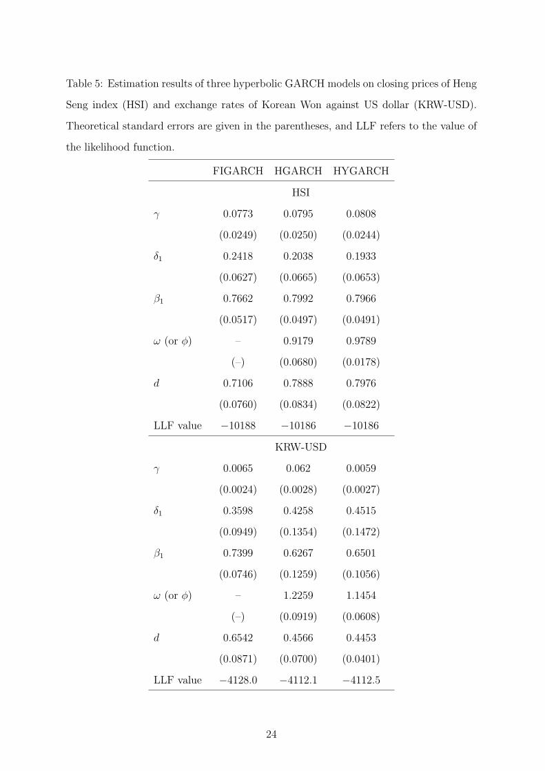
Table 5: Estimation results of three hyperbolic GARCH models on closing prices of Heng

Seng index (HSI) and exchange rates of Korean Won against US dollar (KRW-USD).

Theoretical standard errors are given in the parentheses, and LLF refers to the value of

the likelihood function.

FIGARCH HGARCH HYGARCH

HSI

γ 0.0773 0.0795 0.0808

(0.0249) (0.0250) (0.0244)

δ1 0.2418 0.2038 0.1933

(0.0627) (0.0665) (0.0653)

β1 0.7662 0.7992 0.7966

(0.0517) (0.0497) (0.0491)

ω (or ϕ) – 0.9179 0.9789

(–) (0.0680) (0.0178)

d 0.7106 0.7888 0.7976

(0.0760) (0.0834) (0.0822)

LLF value −10188 −10186 −10186

KRW-USD

γ 0.0065 0.062 0.0059

(0.0024) (0.0028) (0.0027)

δ1 0.3598 0.4258 0.4515

(0.0949) (0.1354) (0.1472)

β1 0.7399 0.6267 0.6501

(0.0746) (0.1259) (0.1056)

ω (or ϕ) – 1.2259 1.1454

(–) (0.0919) (0.0608)

d 0.6542 0.4566 0.4453

(0.0871) (0.0700) (0.0401)

LLF value −4128.0 −4112.1 −4112.5

24

Table 6: Out-of-sample coverage rates of the lower and upper 95% predictive intervals,

the unconditional coverage test statistic (UCTS) and the conditional coverage test statis-

tic (CCTS) for daily closing prices of Heng Seng index (HSI). The p-values are given in

the parentheses.

UCTS CCTS coverage rates(%)

1-day-ahead Lower Upper Lower Upper Lower Upper

FIGARCH 0.6592 0.1645 0.7221 2.3881 94.2 95.4

(0.4169) (0.6850) (0.6970) (0.3030)

HGARCH 1.0134 0.1645 1.0369 2.3881 94 95.4

(0.3141) (0.6850) (0.5954) (0.3030)

HYGARCH 1.4386 0.1645 1.4418 2.3881 93.8 95.4

(0.2304) (0.6850) (0.4863) (0.3030)

5-day-ahead

FIGARCH 0.0242 0.3336 2.3449 2.3808 95.16 95.56

(0.8765) (0.5635) (0.3096) (0.3041)

HGARCH 0.2094 0.2094 1.6156 0.3985 94 .56 94.56

(0.6472) (0.6472) (0.4458) (0.8193)

HYGARCH 0.2094 0.2094 1.6156 0.3985 94 .56 94.56

(0.6472) (0.6472) (0.4458) (0.8193)

10-day-ahead

FIGARCH 0.5519 0.9257 4.0405 2.7154 95.72 95.72

(0.4575) (0.3360) (0.1326) (0.2572)

HGARCH 0.0949 0.2777 3.9644 2.4432 94.70 95.32

(0.7581) (0.5982) (0.1378) (0.2948)

HYGARCH 0.0949 0.2777 3.9644 2.4432 94.70 95.32

(0.7581) (0.5982) (0.1378) (0.2948)

22-day-ahead

FIGARCH 0.3855 5.0393 3.7612 5.9456 95.62 96.87

(0.5347) (0.0248) (0.1525) (0.0512)

HGARCH 0.1891 0.1632 6.7769 2.3858 94.57 95.20

(0.6637) (0.6863) (0.0338) (0.3033)

HYGARCH 0.1891 0.1632 6.7769 2.3858 94.57 95.20

(0.6637) (0.6863) (0.0338) (0.3033)

25

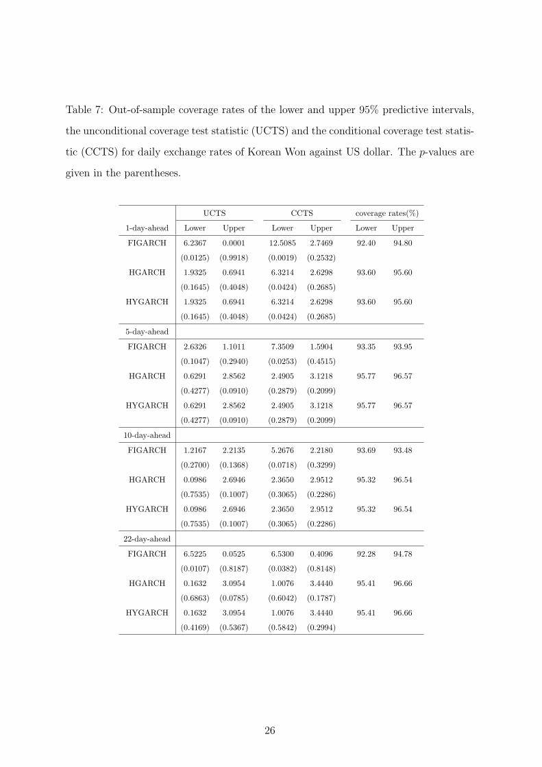
Table 7: Out-of-sample coverage rates of the lower and upper 95% predictive intervals,

the unconditional coverage test statistic (UCTS) and the conditional coverage test statis-

tic (CCTS) for daily exchange rates of Korean Won against US dollar. The p-values are

given in the parentheses.

UCTS CCTS coverage rates(%)

1-day-ahead Lower Upper Lower Upper Lower Upper

FIGARCH 6.2367 0.0001 12.5085 2.7469 92.40 94.80

(0.0125) (0.9918) (0.0019) (0.2532)

HGARCH 1.9325 0.6941 6.3214 2.6298 93.60 95.60

(0.1645) (0.4048) (0.0424) (0.2685)

HYGARCH 1.9325 0.6941 6.3214 2.6298 93.60 95.60

(0.1645) (0.4048) (0.0424) (0.2685)

5-day-ahead

FIGARCH 2.6326 1.1011 7.3509 1.5904 93.35 93.95

(0.1047) (0.2940) (0.0253) (0.4515)

HGARCH 0.6291 2.8562 2.4905 3.1218 95.77 96.57

(0.4277) (0.0910) (0.2879) (0.2099)

HYGARCH 0.6291 2.8562 2.4905 3.1218 95.77 96.57

(0.4277) (0.0910) (0.2879) (0.2099)

10-day-ahead

FIGARCH 1.2167 2.2135 5.2676 2.2180 93.69 93.48

(0.2700) (0.1368) (0.0718) (0.3299)

HGARCH 0.0986 2.6946 2.3650 2.9512 95.32 96.54

(0.7535) (0.1007) (0.3065) (0.2286)

HYGARCH 0.0986 2.6946 2.3650 2.9512 95.32 96.54

(0.7535) (0.1007) (0.3065) (0.2286)

22-day-ahead

FIGARCH 6.5225 0.0525 6.5300 0.4096 92.28 94.78

(0.0107) (0.8187) (0.0382) (0.8148)

HGARCH 0.1632 3.0954 1.0076 3.4440 95.41 96.66

(0.6863) (0.0785) (0.6042) (0.1787)

HYGARCH 0.1632 3.0954 1.0076 3.4440 95.41 96.66

(0.4169) (0.5367) (0.5842) (0.2994)

26