A NEW MATRIX THEOREM AND ITS APPLICATION FOR ESTABLISHING INDEPENDENT COORDINATES FOR COMPLEX DYNAMICAL SYSTEMS WITH CONSTRAINTS

by IVillium C. Walton, Jr., und Earl C. Steeues

LangZey Research Center

N A T I O N A L A E R O N A U T I C S A N D S P A C E A @ M , i N I S T R A T I O N . . W A S H I N G T O N , D . C. OCTOBER 1969 ... .

. . . . . . . .

https://ntrs.nasa.gov/search.jsp?R=19690029270 2018-09-06T14:28:29+00:00Z

TECH LIBRARY KAFB, NY

1. Report No. I 2. Government Accession No. NASA TR R-326 I

4. T i t le and Subt i t le A NEW MATRIX THEOREM AND ITS APPLICATION FOR ESTABLISHING

INDEPENDENT COORDINATES FOR COMPLEX DYNAMICAL SYSTEMS I

-~ WITH CONSTRAINTS - ~~ "___ 7. Authods)

Wil l iam C. Walton. Jr., and Ear l C. Steeves

9. Performing Orgonizotion Name and Address

NASA Langley Research Center

Hampton, Va. 23365

I 12 . Sponsoring Agency Name ond Address

National Aeronautics and Space Administrat ion

Washington, D.C. 20546

15. Supplementory Notes

3. Recip ient 's Cata log No.

5. Report Date October 1969

6. Performing Organization Code

8. Performing Organization Report No. L- 6052

I O . Work U n i t No. 124-08- 13-04-23

11. Contract or Grant No.

13. Type o f Report and Period Covered

Technical Report

14. Sponsoring Agency Code

"

16.

~~

Abstract

A new method is presented by which equat ions of mot ion of a l inear mechanical system can be derived

in terms of independent coordinates when the system is described in te rms of coordinates which are not inde-

pendent but instead are governed by l inear homogeneous equations of const ra in t . There is a discussion of t he

o r ig in in practical vibrat ions analysis of dynamical systems involving equations of constraint. Methods pre-

v iously used for handl ing such systems are d iscussed and the new method i s demonstrated to have the fol-

lowing advantages: (1) For the most general constraint equations, solut ion of the equations is reduced in

substance to comput ing t h e eigenvalues and eigenvectors of a symmetr ic matr ix; and (2) the method is appl i-

cable when there are redundancies in the equat ions of constraint .

I 17. Key Words Suggested by Author(s) ." . - .

Constraints

Equat ions of constraint

Solut ion of equations of cons t ra in t

18. Distribution Statement

Unclassified - Unl imited

Linear equations . . ~~~ ~

19. Securi ty Classif . (of this Clossif . (of this page) 22. Pr ice" 21. No. of Pages

Unclassified Unclassified

*For sale by the Clear inqhouse for Federal Scient i f ic and Technical Informat ion

$3.00 2 1

~ ~~~ . " _"

Spr ingf ie ld, Virginia 22151

A NEW MATRIX THEOREM AND ITS APPLICATION FOR

ESTABLISHING INDEPENDENT COORDINATES FOR COMPLEX

DYNAMICAL SYSTEMS WITH CONSTRAINTS

By William C. Walton, Jr., and Ear l C. Steeves Langley Research Center

SUMMARY

A new method is presented by which equations of motion of a linear mechanical system can be derived in terms of independent coordinates when the system is described in terms of coordinates which are not independent but instead are governed by linear homogeneous equations of constraint. There is a discussion of the origin in practical vibrations analysis of dynamical systems involving equations of constraint. Methods previously used for handling such systems are discussed and the new method is demon- strated to have the following advantages: (1) For the most general constraint equations, solution of the equations is reduced in substance to computing the eigenvalues and eigen- vectors of a symmetric matrix; and (2) the method is applicable when there are redun- dancies in the equations of constraint.

INTRODUCTION

The purpose of this paper is to present a method by which equations of motion of a linear mechanical system can be derived in terms of independent coordinates when basic information about the system is available in terms of coordinates which are not inde- pendent but instead are governed by linear homogeneous equations of constraint. Neces- sity for this derivation occurs frequently in practical vibration analysis. It arises naturally in studies of the motions of bodies composed of components which have been idealized as separate bodies. Experience in analyses of vibrations of engineering struc- tures has convinced the authors that this method often offers decided advantages in prac- tical computation over methods previously used.

The method is based on a mathematical theorem designated the "zero eigenvalues theorem" which allows the computational procedures to be systematically developed. A search of the mathematical literature has been made and nowhere has this result been found .

The paper begins with a background note on dynamical systems involving constraint equations. A brief discussion of approaches previously taken in treating such systems follows. The zero eigenvalues theorem is proved, and the method of this paper is dis- cussed. There is a development of the relationship between the result obtained by the method of this paper and the result obtained by the method generally taught in engineering textbooks. Two examples of application of the theorem to problems from vibration anal- ysis are presented and the numerical considerations involved in practical computing with the method are discussed.

A

B

C

D

E

Fn

G

H

I

K

- K

L

2

M

SYMBOLS

an R X R partitional submatrix of matrix C

an R X (P - R) partitional submatrix of matrix C

a constant matrix of order R X P

a constant matrix defined by equation (23)

a constant matrix defined by equation (14)

elements of vector Q in first example

number of positive finite elements of diagonal matrix h

any nonsingular matrix of order P - G

identity matrix

stiffness matrix referred to coordinates q

stiffness matrix referred to coordinates ;i

Lagrangian

length of cylinder

mass matrix referred to coordinates q

2

- M

m

N

n

P

P

Q

Q

qm ,4 -

R

- T

mass matrix referred to coordinates ;i

axial wave number

number of elements in vector q

subscript denoting general element in vector q

number of elements in vector 6

subscript denoting general element in vector i

generalized forces referred to coordinates q

generalized forces referred to coordinates i j

a vector whose elements are independent coordinates

a vector whose elements are dependent coordinates

a partition of 6 containing R elements

a partition of ;i containing those elements not in ,(a)

coordinates associated with axisymmetric circumferential harmonic

coordinate associated with fourth circumferential harmonic

number of rows in matrix C

radius of cylinder

quadratic form defined by equation (19)

a constant matrix in equation (33c) relating the coordinates i to the coordinates q

matrix defined by equation (35)

3

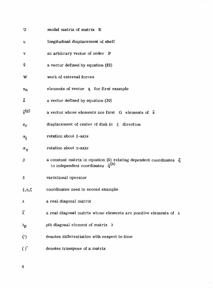
U

U

V

- V

W

ZC

a TJ

P

6

modal matrix of matrix E

longitudinal displacement of shell

an arbitrary vector of order P

a vector defined by equation (22)

work of external forces

elements of vector q for first example

a vector defined by equation (30)

a vector whose elements are first G elements of ii

displacement of center of disk in 5 direction

rotation about [-axis

rotation about q-axis

a constant matrix in equation (9) relating dependent coordinates 4 to independent coordinates q - (b)

variational operator

coordinates used in second example

a real diagonal matrix

a real diagonal matrix whose elements are positive elements of X

pth diagonal element of matrix X

denotes differentiation with respect to time

denotes transpose of a matrix

4

1 1 denotes a row matrix

C l denotes a rectangular matrix

0 denotes a column matrix

BACKGROUND

In conventional analyses of small forced oscillations of mechanical systems, the physical system is idealized so that its configuration at any instant is determined by specification of a finite number of independent coordinates ql, q2, . . ., qn, . . ., qN. Then, with approximations allowable because of the assumed smallness of the oscillations, the Lagrangian of the system may be expressed as in reference 1 in the form

where

(1) q is a column matrix the elements of which are the coordinates q,

(2) M and K are constant symmetric matrices of order N

(3) A prime denotes the transpose of a matrix

(4) A dot denotes differentiation with respect to time.

When the Lagrangian has the form shown by equation (1) and the coordinates qn a r e independent, Lagrange’s equations of motion of the system have the form (see ref. 1):

M i + Kq = Q (2)

In equation (2) Q is a column matrix with N elements. The elements of Q a r e usually called generalized forces. The generalized forces are determined by the fol- lowing requirements: Let 6q be an arbitrary infinitesimal variation of the coordinates composing the matrix q. Then the work W done by the forces applied to the system when these forces act through the displacements produced by the variation shall be given by the equation

W = Q’ 6q (3)

The generalized forces may be functions of the coordinates qn and/or the time explicitly.

Once the equations of motion a r e known in the form indicated by equation (2), there is a well-established and very effective body of mathematical theory and computational

5

technique for determining the behavior of the system. Often, however, it is much eas- ier to express L and W in t e rms of coordinates which a r e not independent but which are governed by linear homogeneous equations of constraint. (See ref. 2.) Let dl, ij2, . . ., qp, . . ., Qp represent such a set of coordinates. The constraint equa- tions then take the form

-

cs = 0 (4)

where ;i is a column matrix the elements of which are the coordinates (Tp, and where C is a constant matrix which has P columns and is, in general, rectangular.

In t e rms of the dependent coordinates ip, the Lagrangian will take the form

where and E are symmetr ic matr ices of order P. The work W can be found in the form

w=$ (6)

where 6s is an arbitrary variation of s compatible with the equations of constraint (eq. (4)) and a is a column matrix with P elements which are functions of the coor- dinates sp and/or the time explicitly.

It is useful to know a systematic procedure by which equations of motion in t e rms of independent coordinates, as in equation (2), can be derived by starting with the Lagrangian L and the work W in t e rms of coordinates governed by homogeneous equations of constraint as in equations (5) and (6). The object of this paper is to set forth such a procedure, but before doing so, it is appropriate to discuss briefly how the prob- lem has been solved previously.

PREVIOUS METHODS

In the past, the equations of motion in t e rms of independent coordinates have been determined in two ways:

(1) Through consideration of particular physical or geometrical aspects of a prob- lem, the dependent coordinates sp a r e chosen to impart a very simple form to the equa- tions of constraint, which renders easy and obvious determinations of the independent coordinates.

(2) By using one of many variants of Gauss's classical elimination algorithm, the equations of constraint are solved as simultaneous equations; these solutions lead to the selection of certain of the coordinates as independent coordinates and the expression of the remaining coordinates in terms of those which have been selected to be independent.

6

Under the first category of approaches come, for example, those finite-element methods of structural analysis in which the coordinates of a free-body element are dis- placements and rotations at juncture points among structural elements. In such anal- yses the equations of constraint are equalities among appropriate displacements and rotations at junctures and equations in which appropriate displacements and rotations are set equal to zero at junctures where there are supposed to be rigid constraints. A set of independent coordinates is determined by the simple expedient of using a single symbol for each set of displacements and rotations which a r e equated. (See, for example, ref. 3.) This idea is the basis of the now widely used procedure of superimposing stiff- ness matrices or mass matrices of structural elements to determine a stiffness matrix or a mass matrix of an entire structure composed of the connected elements.

In order to illustrate some advantages of the method to be presented, the method generally taught in engineering textbooks is discussed formally. (See, for example, ref. 4.) This method belongs in the second category of approaches. It is assumed (usu- ally tacitly) that the rank R of the matrix C is equal to the number of rows in C and that, therefore, equation (4) may be written as

where

(1) A is an R X R nonsingular constant matrix the columns of which a r e R distinct columns of C

(2) B is an R X . ( P - R) constant matrix the columns of which are those columns of C not included in A

(3) G(a) and a r e column matrices the elements of which are elements of i corresponding to the columns in A and B, respectively. The goal is to establish the coordinates in $b) as independent coordinates.

By renumbering the coordinates ip, it can be arranged that the first R columns of C constitute the matrix A and the last P - R columns of C constitute the matrix B. Correspondingly, the elements of $a) would be the first R elements of <, and the elements of c(b), the last P - R elements of 6. For convenience in the ensuing discussion, it is assumed that such a rearrangement has been made. However, as a practical matter, it is very important to note that in order to actually make a suit- able rearrangement, one must be able to identify R linearly independent columns of C. This identification may not be easy.

Since A is nonsingular, an inverse of A exists and is unique. Equation (7) is satisfied therefore if, and only if,

c(a) = -A-lS(b) (8)

7

where A-l is the inverse of A. It follows that the equat.ions of constraint (eqs. (4)) are satisfied i f , and only i f ,

where

In equation (10) I is an identity matrix of order P - R. Thus, the matrix p is a P x (P - R) matrix.

Substitution of equation (9) into equations (5) and (6) gives an expression for the Lagrangian L and the work W in terms of independent coordinates and in the forms shown by equations (1) and (3) , respectively. The components of the expressions are

where it is to be considered that the substitutions from equation (9) have made the ele- ments of the matrix functions of the coordinates qn and/or the time explicitly.

It is noted that the matrices M and K thus derived are symmetric. For empha- sis, it is pointed out once more that applicability of this method is restricted to the case where the rank R of the matrix C is equal to the number of rows of C and that as a practical matter in the application, one is required to identify R linearly independent columns of the matrix C.

It is of interest to consider at this point the situation where contrary to the assump- tion made in the foregoing discussion, the rank R of C is less than the number of rows of C. It is natural for an analyst in idealizing a physical system to try to specify only the minimum number of equations necessary to define the system. In this event the rows of C are linearly independed and consequently the rank of C equals the number of rows. However, in stress and vibration analyses of engineering structures, experience is showing that it is possible to specify inadvertently equations which repeat the content of equations or combinations of equations previously written. In fact, it can be of great convenience to be able to accept redundant equations as may be seen from one of the examples given subsequently. Not much has been written on practical methods for

8

solving systems with dependent equations. However, reference 5 provides a good illus- tration of how dependent equations of constraint may arise in practice and also a brief discussion of an elimination approach used to solve them.

ZERO EIGENVALUES THEOREM

The objective is to prove a theorem that is the foundation of the method of this paper. Consider the equation

cij = 0 (1 3)

where C is a matrix with any number of columns and any number of rows. Let P be the number of columns and R the number of rows.

Let a square matrix E of order P be defined by the equation E = C'C (14)

(It may be noted that the determinant of E is the Gramian of the vectors comprising the columns of C. (See ref. 6.)) By transposing both sides of equation (14) and using the familiar rule for transposing products of matrices, it follows that

E' = C'(C')' = E (1 5)

Therefore, E, being equal to its own transpose, is symmetric.

It is a well-known property of symmetric matrices that there exist orthogonal matrices U of order P satisfying the following equation:

U'EU = X (16)

where X is a real diagonal matrix of order P. By customary usage, an orthogonal matrix having this property is called a modal matrix of E, and the numbers occupying the main diagonal of X are called eigenvalues of E. To say that U is orthogonal means that

u'u = uu' = I

where the identity matrix I is of order P.

Let Xp represent the eigenvalue at the intersection of the pth row and the pth column of X. If any modal matrix of E is given, it is easy to construct a modal matrix of E so that

X 1 2 X 2 2 X 3 2 . . . Z A P (18)

since the positions of the eigenvalues can be reordered simply by reordering the columns of the given modal matrix. Henceforth, in this paper when reference is made to a modal matrix, it is to be understood that the columns are ordered so that inequality (18) holds.

9

The convention of the preceding paragraph being understood, it is well-known that the eigenvalue matrix A associated with a symmetr ic matr ix E is unique; that is, any modal matrix of E when substituted for U in equation (16) produces the same matrix A.

Let v be an arbitrary column matrix with P elements, and let a quadratic expression S be defined by the equation

S = V'EV (19)

Note that equation (19) can be written as s = V'C'CV

or alternatively, by using equations (16) and (17),

S = v'UU'EUU'V = V'hV (2 1)

where U is any modal matrix of E and where - v = u 'v

Equation (20) shows that S cannot be negative for any non null v. Equation (21) shows that there exist non null forms of V which will make S negative i f , and only if , at least one of the eigenvalues Xp is negative. If any choice of V is given, then v given by v = Uf will satisfy equation (22). (See eq. (17).) Therefore, if one or more of the eigenvalues were negative, there would exist forms of v making S negative and this condition would be a contradiction. It follows that the eigenvalues AP are each positive or zero.

Let an R X P matrix D be defined by the equation D = CU

Then from equations (14) and (16), it follows that D'D = x

Let G be the number of the eigenvalues Ap which are positive. Then the last P - G eigenvalues are zero. It follows from equation (24) that D has the partitioned form indicated by the equation

In equation (25) the null matrix 0 is an R X (P - G) matrix and the matrix is an R x G matrix with mutually orthogonal columns so that

J I D D = X (26)

where x is a diagonal matrix the diagonal elements of which are the G positive eigen- values of E as indicated by the .equation

10

By using equation (17), the equations of constraint (eqs. (13)) may be written as

cuu'; = 0 (28) or alternatively

Dz = 0 (29)

It is clear from equation (25) that equation (29) is satisfied if the f irst G elements of 2 are zero whatever the last P - G elements of may be.

Premultiplying both sides of equation (29) by E' and substitution of equation (25) leads to the equation

&) = 0 (31)

where i?(g) is a column matrix the elements of which are the f i rs t G elements of Z. Thus, equation (29) cannot be satisfied unless the first G elements of i? are zero.

Solving equation (30) for S gives the unique solution

s = uz Thus, the following theorem has been proved:

Theorem: Consider any set of linear homogeneous equations c; = 0 (334

and let the symmetric matrix E be defined by

E = C'C ( 3 3b)

The most general solution of the equations may be expressed in the form

S = Tq (334

where T is a matrix whose columns are the columns of any modal matrix of E corresponding to eigenvalues of E which have the value zero, and where q is an arbitrary column matrix conformable with T.

11

COMPUTATIONAL PROCEDURE

With the basic theorem from the preceding section, the following procedural outline may be set forth. It is assumed that the generalized forces in the column matrix a are functions of time alone. (If a is a function of the coordinates cp explicitly, addi- tional substitutions will be required which depend on the functional form of a.) Given:

(1) E and g, both constant symmetric matrices of order P

(2) C, a constant matrix with P columns and any number of rows

(3) a, a column matrix with P elements each of which may be a function of time.

Object:

(1) To compute a matrix T so that:

(a) The transformation 6 = Tq relates the dependent coordinates 6 appearing in equations (5) and (6) to a se t of independent coordi- nates q suitable for use in equation (2)

(b) The transformation Q = T'G produces a matrix Q suitable for use in equation (2)

(2) To compute matrices K and M suitable for use in equations (1) and (2).

Procedure:

(1) Compute E where E = C'C. Then E will be symmetric of order P and positive semidefinite

(2) Compute a modal matrix U and the eigenvalues Xp of the matrix E (where p = 1, 2, 3 , . . ., P). This operation is standard at modern computing installations and, in 'fact, is one of the most successful appli- cations of digital computers

(3) Identify the columns of U which correspond to zero eigenvalues. This step requires attention because in principle one can fairly question the possibility of a rigorous distinction between finite eigenvalues and eigen- values having the value zero when, as is normal, there is any roundoff error in the process by which the eigenvalues are computed. This point is discussed in the section "Comments on Numerical Aspects of Computation''

12

(4) Assemble a matrix the columns of which are the columns of U cor- responding to the eigenvalues having the value zero. This matrix is. the required transformation matrix T. Its dimensions are P by P - G where G is the number of positive eigenvalues of E

(5) Compute K and M by the formulas K = T'KT and M = T'MT. Then K and M will be symmetric.

RELATION TO PREVIOUS METHOD

Equation (33c) gives the most general solution to the equations of constraint (eq. (4)). Since the matrix ij appearing in equation (33c) is completely arbitrary, the solution can just as well be stated in the form

= THq = F q (34)

where H is any nonsingular square matrix of order P - G and where - T = TH (3 5)

In order that a matrix ;I; may be written as in equation (35), it is both necessary and sufficient that the columns of constitute a set of linearly independent eigenvectors of E corresponding to the eigenvalues of E which have the value zero. The eigenvec- tors in 5; will not, in general, be orthonormal nor even orthogonal. The columns of are orthonormal i f , and only i f , H is an orthogonal matrix and orthogonal if H is a diagonal matrix. Proof of these statements will not be made as they amount merely to a formal statement of the basic results of that portion of the theory of matrices which deals with repeated eigenvalues of a real symmetric matrix. (See, for example, ref. 7.) A connection may now be made between the method of this paper and the textbook method as given in reference 4.

By assuming that the column and coordinate rearrangements leading to equation (7) have been carried out, one may write

A'

B'

""-

-

A i B ] = I I

A' A

B' A "-"

13

It follows that

where in equation (37) the matrix on the right is a P X (P - R) null matrix. It is clear from equation (37) that the columns of p are linearly independent eigenvectors of E corresponding to P - R eigenvalues having the value zero. The R X R submatrix A'A is of rank R. The matrix E is consequently of rank R and possesses no more than P - R eigenvalues with value zero.

Thus, the textbook solution, which is a variant of Gauss's classical elimination algorithm, is seen to be a s.olution of the form of equation (34).

FIRST EXAMPLE

In the first example, the method of this paper is applied .to derive the equations of motion of a simple chain of spring-mass elements. The main intent is to illustrate an application of the method. However, some points of general interest arise.

The system consists of five point masses connected by linear massless springs as shown in sketch (1). Each of the masses and each of the spring constants are assumed to have unit magnitude. The masses may displace only in the horizontal direction and the displacement of the nth mass referred to its undeformed position is denoted by X,. A

positive vaiue of Xn is taken to mean displacement to the right, and a negative value, displacement to the

1 2 3 4 5 left. A horizontal external force Fn, positive to the

Sketch (l).- Spring-mass system. right and a function of time only, acts upon the nth mass.

The five displacements constitute a se t of independent coordinates which determine the configuration of the system at any instant; and in t e r m s of these coordinates, it is easy to write down directly equations of motion of the system in the form

14

where

K =

- 1 - 1 0 0 0

-1 2 -1 0 0

0 -1 2 -1 0

0 0 -1 2 -1

0 0 0 - 1 1 L

1 0 0 0 0

0 1 0 0 0

0 0 0 1 0

0 0 0 0 1 Q=F] F5

Equation (38) has the form of equation (2). Thus, from a practical point of view, the method of this paper is not needed for an analysis of the system since the end result of the method, equations of motion in t e r m s of indepen- r\nrv~1 dent coordinates, is readily obtained by inspection. However, since the object is to illustrate the method, let the system be viewed in a different way as illus- trated in sketch (2). There the system of sketch (1)

1 2 3 4 5 6 7 8

Sketch (2).- Cut system.

15

is shown figuratively divided into four parts by cuts at the three inner masses to produce an eight-mass system. The half circles represent masses of one-half-unit magnitude. The displacement of the pth mass of this cut system is denoted by 4 P'

It is assumed that three equations of constraint are imposed on the coordinates; namely,

(2 = 93 (404

Thus the coordinates sp are not independent, and from the simple geometric considera- tions involved, it is clear that under these equations of constraint, the systems of sketch (1) and sketch (2) are the same. In terms of the coordinates GP, a Lagrangian of the system may be expressed by an equation like equation (5) with

1 - 1 0 0 0 0 - 1 1 0 0 0 0

E = [ 0 0 0 0 0 0 - 1 0 1 - 1 0 1 0 0 1 - 1 0 0

0 0 0 0 - 1 1 0 0 0 0 0 0 0 0 0 0 0 0

7

0 0 0 0 0 0 0 0 0 0 0 0 1 -1 ,1 1 -

7

1 0 0 0 0 0 0 0 0 1 / 2 0 0 0 0 0 0 0 0 1 / 2 0 0 0 0 0 0 0 0 1 / 2 0 0 0 0 0 0 0 0 1 / 2 0 0 0 0 0 0 0 0 1 / 2 0 0 0 0 0 0 0 0 1 / 2 0 0 0 0 0 0 0 0 1

_I -

The work W for the system may be expressed by an equation following the form of equation (6) with

i t is noted that the form indicated by equation (42) for the matrix a' is not unique. The following form, for example, will serve equally well:

16

All that is required is that ?$ when introduced in equation (6) should yield the work done during any displacement consistent with the equations of constraint.

Equations (40), the equations of constraint, may be put in the form of equation (4) with

p 1 - 1 0 0 0 O O l

c = o o 0 1 - 1 0

l o o 0 0 0 1 - 1 0 O I (44)

The first step in the application of the method is to compute the matrix E defined by equation (14). This computation yields

0 0 0 0 0 0 - 0 1 - 1 0 0 0 ::I

0 - 1 1 0 0 0 0 0 0 0 0 1 - 1 0 0 0 0 0 0 0 0 - 1 0 0 0 1 0 1 - : j

0 0 0 0 0 - 1 1 0 - 0 0 0 0 0 0 0 0

(4 5)

The matrix U which follows is a modal matrix of the matrix E , as may be easily verified by substitution of the matrix into equations (16) and (17).

U =

- 0

1 /E - l/E

0

0

0

0

0 L

0 0 1 0 0 0 0

0 0 0 l /@ 0 0 0

0 0 0 l/fi 0 0 0

l/fi 0 0 0 1 J f i 0 0

-l/@ 0 0 0 l/fi 0 0

0 ljfi 0 0 0 lffi 0

0 - 1 / n 0 0 0 l/fi 0

0 0 0 0 0 0 1

The matrix X containing the eigenvalues associated with the modal matrix is given by

17

I I I I11111 II l111ll1l111

x =

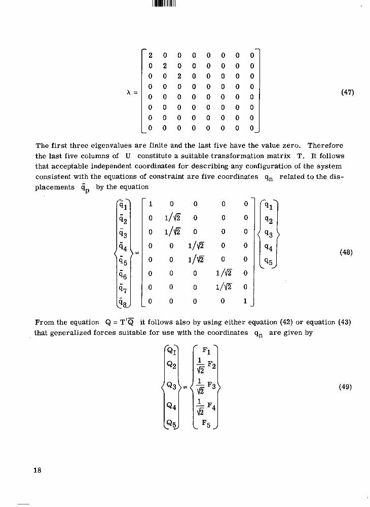
- 2 0 0 0 0 0 0 0 0 2 0 0 0 0 0 0 0 0 2 0 0 0 0 0 0 0 0 0 0 0 0 0 0 0 0 0 0 0 0 0 0 0 0 0 0 0 0 0 0 0 0 0 0 0 0 0 0 0 0 0 0 0 0 0 I

(47)

The first three eigenvalues are finite and the last five have the value zero. Therefore the last five columns of U constitute a suitable transformation matrix T. It follows that acceptable independent coordinates for describing any configuration of the system consistent with the equations of constraint are five coordinates qn related to the dis- placements by the equation P

- 1 0 0

0 l/E? 0 0 0

0 l/E 0 0 0

0 0 1/Jz 0 0

0 0 l/E 0 0

0 0 0 1/Jz 0

0 0 0 1/Jz 0

From the equation Q = T'Q it follows also by using either equation (42) or equation (43) that generalized forces suitable for use with the coordinates qn are given by

18

Completing the steps in the method gives

I 1

1 0 0 1/2 0 0 0 0 0 0

-1/@

-1/a 1

K = T'KT = o - 1/2

0 0

L o 0

0 0 0 0 0 0 1/2 0 0 0 1/2 0 0 0 1

0 0

-1/2 0

1 - 1/2

0

0

0

-

-1/2 1 -l/fi

0 -1fJz 1

Equations (49), (50a) and (50b) give all the quantities necessary for writing the equations of motion for the spring-mass system in the form of equation (2). By use of equation (48), solutions of the equations giving time histories of the coordinates qn can be transformed into time histories of the original coordinates cjp. If initial conditions consistent with the equations of constraint are given in t e rms of the coordinates spy the equations

q = T'q (51) and

q = T'G (52)

may be used to convert them into initial conditions on the coordinates qn.

It may be noted that the matrices K, My and Q given in equations (50b), (50a), and (49) are not identical to the corresponding matrices in equations (39) which were written down directly from simple physical considerations. Either set of matrices forms a valid basis for equations of motion of the system of sketch (1). The difference between the matrices arises from the fact that the coordinates qn determined by the method of this paper are not related to the coordinates sp in the same way as are the displace- ment coordinates Xn. Equation (48) shows the relationship between the coordinates qn and ip whereas coordinates Xn and ijp are related by the equation

19

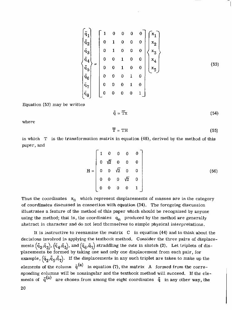
Equation (53) may be written

ij = Tx

7

0

0

0

0

0

0

0

1 -

(53)

where - T = TH (55)

in which T is the transformation matrix in equation (48), derived by the method of this paper, and

H = O O f i O 0

o o o \ I z o 1 0 o o o 1 J

Thus the coordinates X, which represent displacements of masses are in the category of coordinates discussed in connection with equation (34). The foregoing discussion illustrates a feature of the method of this paper which should be recognized by anyone using the method; that is, the coordinates qn produced by the method are generally abstract in character and do not lend themselves to simple physical interpretations.

It is instructive to reexamine the matrix C in equation (44) and to think about the decisions involved in applying the textbook method. Consider the three pairs of displace- ments (G2,G3), (G4,i5), and 96997 straddling the cuts in sketch (2). Let triplets of dis- .placements be formed by taking one and only one displacement from each pair, for example, ({,,c5,i7). If the displacements in any such triplet are taken to make up the

elements of the column in equation (7), the matrix A formed from the corre- sponding columns will be nonsingular and the textbook method will succeed. If the ele- ments of are chosen from among the eight coordinates 6 in any other way, the

20

(- - >

matrix A will be singular. In applying the textbook method to this simple problem, recognition of the combinations of coordinates suitable to form i(a) must come about either from physical insight or from understanding of linear dependence among the col- umns of. C. In applying the method of this paper, it is not necessary to think directly about the physics involved or about the linear dependence. Instead, the problem becomes one of finding a modal matrix of E and identifying the columns associated with eigen- values having the value zero. Because of the block-diagonal form of E in this case, it was possible by inspection to put down exactly a modal matrix and the eigenvalues of E. Therefore, all decisions in the application of the method of this paper could be made eas- ily on a purely mathematical basis.

SECOND EXAMPLE

The purpose of this second example is to show a condition in which redundancies in the equations of constraint arise in a natural way. The mechanical system is shown in sketch (3). A cylindrical elastic shell is fixed at one end to an immovable base. At the other end, a thin massive rigid disk is attached to the wall of the shell by four pins placed at 90° intervals around the circumference. Points in the shell wall are assumed to displace only longitudinally.

pin\F-< Disk

Sketch (3).- Shell with attached disk.

By adopting an approximation common in practical vibration analysis, the longi- tudinal displacement u of a general point in the shell wall is expressed as a linear com- bination of a finite number of displacement functions. The expansion assumed is

where m takes on positive integral values and the summation sign indicates summation of the terms corresponding to some finite number of selected values of m. The coeffi- cients tj and a r e functions of time alone and serve as coordinates which describe the instantaneous configuration of the shell.

m,o m,4

By assuming small displacements, the instantaneous position of the disk is deter- mined by specification of three coordinates zc, at, and aq defined as follows:

(1) zc is the displacement of the center of the disk parallel to the longitudinal axis of the shell

(2) at and aq are small rotations about axis 5 and q, respectively, as shown in sketch (3) .

Equating the displacements of the disk to the displacements of the shell at each of the four pins gives

I

where r is the radius of the cylinder. If, in the summation on the right, only the terms corresponding to m = 1 are retained, the equations may be put in the form

cs = 0

where

1 0 -1 -1 -1

1 1 0 -1 -1

1 0 1 -1 -1

1 -1 0 -1 -1

c = [ -

(59)

22

and

It will be clear on inspection that an attempt to determine independent coordinates for this system by a straightforward application of the textbook method must fail because any choice of the matrix A will lead to a matrix which has at least two proportional columns and which is therefore singular. This difficulty stems from the fact that the system of equations is redundant; the redundancy may be demonstrated by adding rows 1 and 3 of matrix C and subtracting row 2 from the result to produce row 4.

One way to determine independent coordinates would be to discard the fourth equa- tion from the system and apply the textbook method to the first three equations. However, this approach requires, in general, the following:

(1) Recognition in the first place that the system is redundant

(2) Identification of dependent equations

(3) Identification of a nonsingular submatrix A after redundant equations are discarded.

For the example problem under consideration, the required understanding of the structure of the equations may be gained by inspection. In practical work, however, there may be many equations of constraint involving many unknowns, and the coefficients making up the matrix C will usually not be small integers. Generally, in such situations, little of use can be deduced about the system merely by inspection of the matrix of coefficients. Also, one cannot always rely on physical insight to detect and understand redundancies. Furthermore, there are considerable theoretical and practical difficulties in making com- putational tests for redundancy when there is er ror , such as roundoff e r ror , in the process by which the coefficients of the equations of constraint are generated. (See ref. 5.)

Proceeding now to apply the method of this paper yields the matrix E as -

4 0 0 -4 -4 0 2 0 0 0 0 0 2 0 0 - 4 0 0 4 4

- - 4 0 0 4 4

23

The eigenvalues of E are

x1= 12 x2 = 2

x4 = 0 x3 = 2 I x g = 0 i

It may be easily verified that the two columns of the matrix T which follow are ortho- normal eigenvectors of E corresponding to the two eigenvalues X4 and X5 which have the value zero.

0 0

T = 0 0

-116 llhi

Therefore the system may be described by two independent coordinates q1 and q2 related to the coordinates in 6 by the equation

4 = Tq (6 5)

As can be seen, direct concern with the number and nature of redundancies in the equations of constraint is unnecessary when the method of this paper is used. The prob- lem reduces in substance to that of determining a modal matrix of E and identifying the columns which correspond to eigenvalues with the value of zero.

COMMENTS ON NUMEFUCAL ASPECTS O F COMPUTATION

In the examples it was possible to,put down exactly the matrix C, to carry out exactly the multiplication C'C to produce the matrix E, and to determine exactly the eigenvalues of E and orthonormal eigenvectors corresponding to the eigenvalues with value zero. In practical work, however, numerical error due to roundoff and/or trunca- tion may be introduced at any of these three stages of calculation. The extreme effect of such e r rors would, of course, be complete loss of numerical significance in the digits representing the eigenvalues of E and the elements of the eigenvectors of E. In the event the computation is subject to serious loss of significance, the matrix C is said to be "ill-conditioned" with respect to the computing process used. The best indication of ill-conditioning is sensitivity of final results to small changes in the elements of C. The authors have applied the method of this paper a number of times in practical vibration

24

analysis and have not encountered a situation in which the matrijr C is ill-conditioned. From general experience, however, the possibility of ill-conditioning must be anticipated whenever simultaneous equations are solved numerically, and the method of this paper presents no exception to this statement. When an ill-conditioned system arises, the recourse most often open is to increase the number of digits carried in the computation. If this procedure is attempted in connection with the method of this paper, it should be recognized that it may be necessary to increase the carried significant figures in the stage of the calculation in which the elements of C are generated as well as in the implementation of the multiplication C'C and in the calculation of the eigenvalues and eigenvectors of E.

Another consequence of numerical error is that finite numbers may be generated for eigenvalues of E which would be precisely zero if there were no error in the com- puting process. Thus, the question is raised, in principle at least, of the possibility of rigorous distinction between finite numbers representing finite eigenvalues of E and finite numbers representing eigenvalues of E which are, in fact, zero. In the authors' experience this possibility has not proved to be a problem in practice. The authors use the threshold Jacobi method (ref. 8) to compute the eigenvalues and a modal matrix of E. Approximately 15 significant figures are carried throughout the calculation. With this procedure, inspection of the eigenvalues computed for E has always revealed two clearly distinguishable sets of numbers, the numbers in one set being many orders of magnitude smaller than the numbers in the other set. The set of numbers with relatively large magnitudes are regarded as finite eigenvalues, and the remaining numbers are con- sidered to be eigenvalues with value zero.

It is not difficult to show that the number of finite eigenvalues of E is equal to R, the rank of C. Frequently, R is known from physical or geometric considerations. In particular, it often occurs that one knows that the equations of constraint are linearly independent in which case the rank R of C is equal to the number of rows of C. Such advance information, of course, enhances confidence in the identification of zero eigenvalues.

The purpose of this paper is to present a new method by which equations of motion of a linear mechanical system can be derived in terms of independent coordinates when the Lagrangian of the system and the generalized forces are expressed with r-eference to coordinates which are not independent but instead are governed by linear homogeneous equations of constraint.

25

As background, there are recalled well-known mathematical forms of the Lagrangian and the work statement associated with small oscillations of mechanical systems. When the coordinates utilized to develop these expressions are independent, Lagrange's method may be applied to determine differential equations of motion of the system in a form which has been well studied and is subject to powerful methods of solution. However, as a matter of convenience, practical analysis frequently starts with coordinates which a r e dependent by virtue of the imposition of linear homogeneous equations of constraint. Thus, it isuseful to know a relationship by which the dependent coordinates can be transformed into a set of independent coordinates.

Next, there is a discussion of methods previously used for constructing a t rans- formation from dependent to independent coordinates. In one category of analysis, the dependent coordinates are chosen to impart a very simple form to the equations of con- straint s o that the transformation may be written from inspection. In a second category of approaches based on Gaussian elimination, some of the original dependent coordinates are selected to be independent coordinates and those of the original coordinates remaining are related to those selected to be independent. This procedure has the drawback that it requires in effect the identification of a square nonsingular submatrix in the matrix of the coefficients of the equations of constraint.

The third part of the paper is devoted to the basic result, a theorem which se rves as a foundation for a new method for constructing the transformation from independent to dependent coordinates.

Theorem: Let a real symmetric matrix be constructed by multiplying the matrix of coefficients in the equations of constraint by the transpose of the same matrix. Consider any modal matrix of the symmetric matrix so defined and select from the modal matrix the columns corresponding to eigenvalues with value zero. Then the matrix of these columns is a legitimate transfor- mation relating the original dependent coordinates to a set of independent coordinates.

The advantages of constructing the transformation matrix by this method are (1) compu- tation is reduced essentially to generating a modal matrix and the eigenvalues of a real symmetric matrix and (2) the method is applicable to systems where there are redundant equations among the equations of constraint.

Computing procedures for applying the method are given in outline form, the method is applied to two simple physical problems, and numerical considerations in the applica- tion of the method are discussed. Also a connection is made between the method of this paper and the method generally given in engineering textbooks. In addition to illustrating

26

1

the method, the examples bring out the abstract nature of the coordinates produced by the method and indicate how redundancies in the equations of constraint may arise in practical vibration analyses.

Langley Research Center , National Aeronautics and Space Administration,

Langley Station, Hampton, Va., August 11, 1969.

REFERENCES

1. Goldstein, Herbert: Classical Mechanics. Addison-Wesley Publ. Co., Inc., c.1950.

2. Hurty, Walter C.: Dynamic Analysis of Structural Systems Using Component Modes. AIM J., vol. 3, no. 4, Apr. 1965, pp. 678-685.

3. Przemieniecki, J. S.: Theory of Matrix Structural Analysis. McGraw-Hill Book Co., c.1968.

4. Hurty, Walter C.; and Rubinstein, Moshe F.: Dynamics of Structures. Prentice-Hall, Inc., c.1964.

5. Greene, B. E.; Jones, R. E.; McLay, R. W.; and Strome, D. R.: On the Application of Generalized Variational Principles in the Finite Element Method. AIAA Paper No. 68-290, Apr. 1968.

6. James, Glenn; and James, Robert C., eds.: Mathematics Dictionary. D. Van Nostrand Co., Inc., c.1959.

7. Hildebrand, F. B.: Methods of Applied Mathematics. Prentice-Hall, Inc., 1952.

8. White, Paul A.: The Computation of Eigenvalues and Eigenvector of a Matrix. J . SOC. Indust. Appl. Math., vol. 6, no. 4, Dec. 1958, pp. 393-437.

NASA-Langley, 1969 - 19 L-6052

I ~

27

NATIONAL AERONAUTICS AND SPACE ADMINISTRATION WASHINGTON, D. C. 20546

OFFICIAL BUSINESS FIRST CLASS MAIL w POSTAGE A N D FEES PAID

NATIONAL AERONAUTICS AP. SPACE ADMINISTRATION

I'

POSTMASTER: If Undeliverable (Section 158 Postal Manual) D o Not Recur

"The aerommtical and space nctivlties of the Ugzited Stntes shnll be colzdmted so as t o contr{bute . . . to the expansion of hu71za?z knozul- edge of pheaonzenu in the ntvtosphese mzd space. T h e Adminis/rntion shnll provide for the widest pmcticnble mzd appropriate dissenliantioa of infosn~ntion concerlaing its nctiflities alzd the resalts thereof."

-NATIONAL AERONAUTICS AND SPACE ACT OF 1958

NASA SCIENTIFIC AND TECHNICAL PUBLICATIONS

TECHNICAL REPORTS: Scientific and TECHNICAL TRANSLATIONS: Information technical information considered important, published in a foreign language considered complete, and a lasting contribution to existing to merit NASA distribution in English. knowledge.

SPECIAL PUBLICATIONS: Information TECHNICAL NOTES: Information less broad derived from or of value to NASA activities. in scope but nevertheless of importance as a contribution to existing knowledge.

TECHNICAL MEMORANDUMS: Information receiving limited distribution because of preliminary data, security classifica- tion, or other reasons.

CONTRACTOR REPORTS: Scientific and technical information generated under a NASA contract or grant and considered an important contribution to existing knowledge.

Publications include conference proceedings, monographs, data compilations, handbooks, sourcebooks, and special bibliographies.

TECHNOLOGY UTILIZATION PUBLICATIONS: Information on technology used by NASA that may be of particular interest in commercial and other non-aerospace applications. Publications include Tech Briefs, Technology Utilization Reports and Notes, and Technology Surveys.

Details on the availability of these publications may be obtained from:

SCIENTIFIC AND TECHNICAL INFORMATION DIVISION

NATIONAL AERONAUTICS AND SPACE ADMINISTRATION Washington, D.C. 20546