A New Method for Transient Stability Analysis

NAOTO YORINO, TAKESHI SAITO, YOSHIFUMI KAMEI, and HIROSHI SASAKIHiroshima University, Japan

SUMMARY

This paper proposes a brand-new method for tran-sient stability analysis in power systems. The proposedmethod directly computes the critical trajectory for a givencontingency to obtain the critical condition of the studiedsystem. Although the method may be useful for generalnonlinear dynamic systems, it is applied to the problem ofobtaining a controlling UEP, unstable equilibrium point,which provides inevitable information for the energy func-tion methods to assess transient stability. Namely, the pro-posed method effectively yields a critical trajectory onPEBS together with the controlling UEP, thus improvingthe conventional BCU method. The effectiveness of theproposed method is demonstrated in 3-machine 9-bus and6-machine 30-bus systems. © 2007 Wiley Periodicals, Inc.Electr Eng Jpn, 159(3): 26–33, 2007; Published online inWiley InterScience (www.interscience.wiley.com). DOI10.1002/eej.20245

Key words: power system; transient stability; sta-bility assessment; energy function method.

1. Introduction

In recent years, the importance of transient stabilityanalysis has grown as electric power systems have becomelarger and more complex. Furthermore, as a result of liber-alization, real-time analysis is now important, and precise,fast methods for such analysis are needed. Prior methodsfor transient stability analysis include the simulation meth-ods and the energy function methods, each of which is useddepending on conditions. The former can be used to accu-rately determine stability, but are deficient because thecomputational burden is high. The latter have the reversecharacteristics. In contrast, the authors have studied meth-ods to determine stability by calculating directly the gener-ator fluctuation corresponding to the critical case for

stability after fault [1, 2]. Analysis of this generator fluctua-tion represents a problem of finding a solution (in otherwords, a trajectory) for differential equations. As a result,in this paper the authors define the trajectory correspondingto the critical stability as the critical trajectory, and basedon this analysis propose a new method for transient stabilityanalysis.

The proposed method is an entirely new method thatat once finds solutions for the critical trajectory in thetransient stability analysis model and for unstable equilib-rium points. This method may be regarded as a generalmethod for finding critical boundaries in nonlinear systems,but here is applied to the BCU method, one type of energyfunction method, when using it in electric power systemmodels. The BCU method occasionally encounters prob-lems in which the calculation of the unstable equilibriumpoints necessary to calculate the critical energy does notconverge well. However, the authors’ method resolves thisproblem.

2. Critical Trajectory

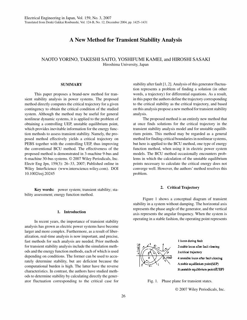
Figure 1 shows a conceptual diagram of transientstability in a system without damping. The horizontal axisrepresents the phase angle of the generator, and the verticalaxis represents the angular frequency. When the system isoperating in a stable fashion, the operating point represents

© 2007 Wiley Periodicals, Inc.

Electrical Engineering in Japan, Vol. 159, No. 3, 2007Translated from Denki Gakkai Ronbunshi, Vol. 124-B, No. 12, December 2004, pp. 1425–1431

Fig. 1. Phase plane for transient states.

26

a stable equilibrium point, and the system is stable in thiscondition (point A). However, when a fault occurs in thesystem, the system state moves away from the stable equi-librium point by tracing a locus trajectory as can be seen inFig. 1 (trajectory 1). If the fault is cleared in a relativelyshort time, then the operating point oscillates (trajectory 2),as can be seen in the figure, and ultimately converges on theoriginal state. However, if a certain amount of time passesafter the fault occurs, then the system does not return to itsoriginal state after the fault is cleared, and instead becomesunstable (trajectory 4). If the fault is cleared within thecritical fault clearance time, then a trajectory resembling 3in the figure appears, and the operating point converges onan unstable equilibrium point (point B) for an infiniteamount of time. The proposed method is a method to findthis critical trajectory efficiently.

3. Conventional Methods

Broadly speaking, methods for transient stabilityanalysis include the simulation method and the energyfunction method.

3.1 Simulation method

This is a method in which the state of the system iscalculated consecutively, and a determination about stabil-ity is made based on behavior. In this method, the state ofthe system can be represented precisely, and analysis of adetailed model that takes into consideration control systemscan also be performed. However, the simulation modelgreatly increases computation time, depending on the com-plexity of the model and the scale of the system. Moreover,the fault clearance time must be set beforehand, and stabil-ity or instability at that point must be determined. As aresult, this method is not useful for finding critical states.In general, critical states must be calculated in order todetermine the stability margin in a system. In this instance,the fault clearance time is set based on trial and error, andthis simulation must be repeated many times.

The proposed method is compared to the simulationmethod in a later section. The state equation below is usedas a system model:

Note that Pei(θ) = Σj=1 YijEiEjsin(θi − θj + αij).ωi: generator angular velocity; ωs: base angle veloc-

ity; θi: internal phase angle; Mi: inertial constant; Pmi:

mechanical input; Pei: electrical output; D: control constant;

Yij: admittance matrix elements; Ei, Ej: internal voltages ofgenerators; αij: constant

3.2 Energy function method

The energy function method is a method that makesstability determinations based on the transient energy val-ues. It is an extremely fast method, but is limited in that themodel in question is restricted.

In the energy function method, the state equation isconverted to change coordinates, as can be seen below:

Note that δi = θi − θ0, ω~

i = ωi − ω0, θ0 = 1 / MT Σi=1n Miθi.

ω0 = 1 / MTΣi=1n Miωi, ω

~: converted generator angularvelocity; δ: converted internal phase angle; Mi: inertiaconstant; Pm: mechanical input; Pe: electrical output;MT = ΣMi; Pcoa(δ) = Σ(Pmi

− Pei(δ)).

The energy function for Eq. (2) is given below:

Here, the first item, VK, represents kinetic energy and thesecond item, VP, represents potential energy, and δi

s repre-sents the equilibrium point after fault.

The energy function method makes determinationsabout stability based on the energy value in Eq. (3). How-ever, it is necessary to calculate the critical energy at this point.The critical energy can be found based on the unstable equi-librium point, but normally there are several unstable equilib-rium points, and only one represents the unstable equilibriumpoint that provides the critical energy. This is referred to as thecontrolling unstable equilibrium point (Controlling UEP orC-UEP). Accurately determining the C-UEP is important fordetermining transient stability precisely.

A method known as the BCU method among energyfunction methods involves finding C-UEP using an energygradient system. In this method, first the trajectory for Eq.(1) during fault (trajectory 1 in Fig. 1) is found usingsimulations, and then the first maximum (Exit Point) for theenergy value VP in Eq. (3) is found. Then, numerical inte-gration is performed along the steepest direction for thevalue VP (in other words, along the tail head), and C-UEPis found. This operation involves finding the gradient sys-tem defined as

(1)

(2)

(3)

27

In other words,

near the unstable equilibrium point by integrating from theExit Point, and then finding C-UEP precisely using the NRmethod.

The numerical integration described above involvesmathematical difficulties because it tries to proceed on astability manifold referred to as a PEBS (Potential EnergyBoundary Surface) for the direction of the unstable equilib-rium point. These mathematical difficulties are equivalentto not being able to find a C-UEP for which a minimumgradient point does not exist or for which a minimumgradient point is not included in the C-UEP convergenceregion. In order to resolve this problem, the Shadowingmethod [6], which corrects the errors during the numericalprocess, has been proposed. Note that practical methods[7–10] which use an approximate critical energy valuewithout finding C-UEP have also been proposed, but cal-culating C-UEP remains an important subject for makingdeterminations about stability in a more precise fashion andfor evaluating stability margin.

Furthermore, after C-UEP is found using the energyfunction method, the critical energy Vcr is calculated asshown below using the value δu, and a determination aboutstability is made:

In general, in the energy function method only determina-tions about the sufficient conditions for stability can bemade, given the effects of damping. However, for the sakeof a comparative evaluation, damping is not taken intoconsideration. In other words, in this paper the authors finda point that satisfies the following equation on the trajectoryδf(t) (trajectory 1 in Fig. 1) during failure and Vcr, and thenfind the critical clearing time tcr:

4. Proposed Method

In this paper, the authors propose a method for tran-sient stability analysis based on the BCU method, a methodrepresentative of the energy function method. In the BCUmethod, finding C-UEP reliably using the numerical inte-gration in Eq. (4) as described above represents an impor-tant issue. As a result, a more stable method referred to asthe Shadowing method has been proposed. However, be-cause the mathematical difficulties described above cannotbe completely resolved, often the desired unstable equilib-rium point cannot be reached. The problem of findingC-UEP is equivalent to the problem of finding the criticaltrajectory 3 in Fig. 1. However, Fig. 1 is drawn with respect

to the system of Eq. (1). The discussion here refers to theproblem of finding the critical trajectory for the system ofEq. (4).

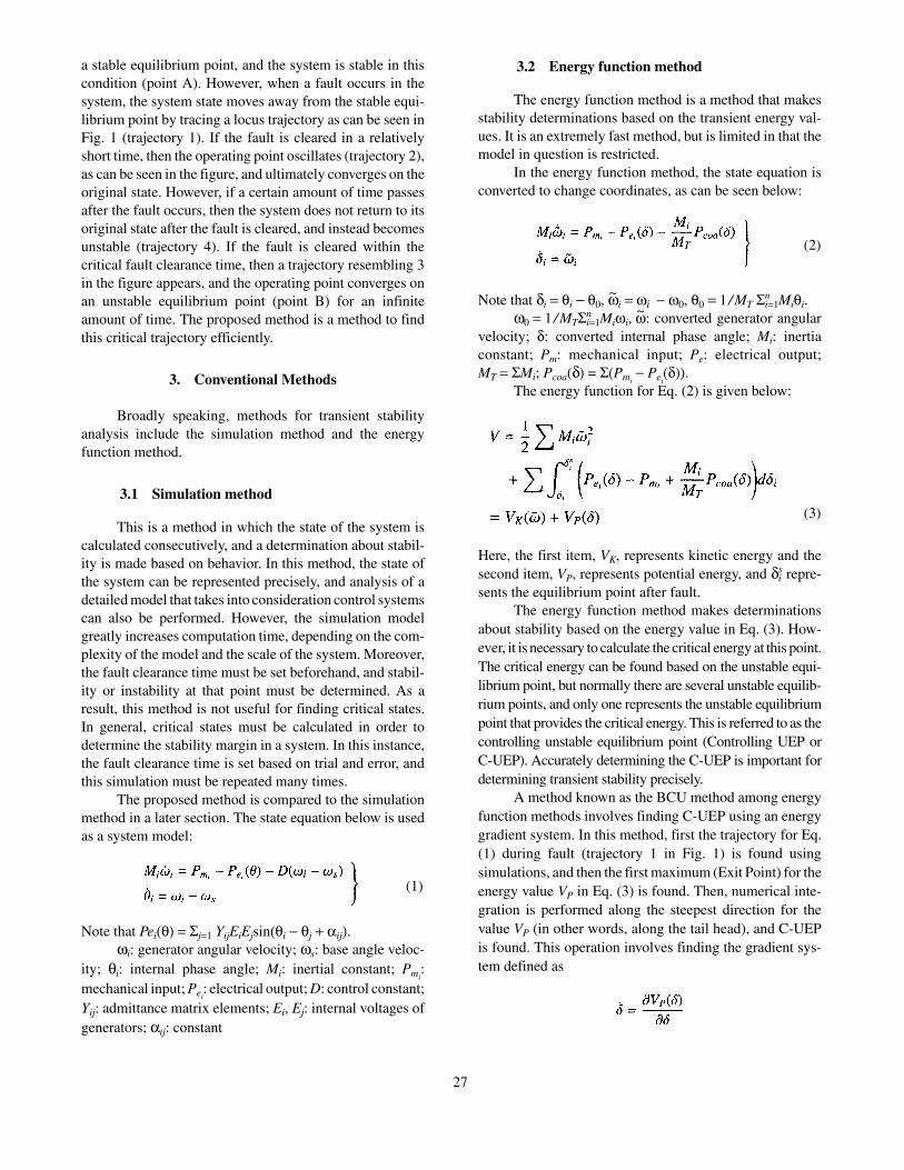
Thus, the authors propose a method to efficiently findthe critical trajectory itself, including the unstable equilib-rium point, instead of finding the critical trajectory usingconsecutive numerical integration. This method is based onthe conditional expressions for the Exit Point, and theunstable equilibrium point, which specify the two boundarypoints of the trajectory. The trajectory is decomposed intomultiple segments with an appropriate length, converting aconventional numerical integration w.r.t. time into that w.r.t.distance, to find simultaneously the trajectory from the ExitPoint to the unstable equilibrium point (refer to Fig. 2).Note that initially the Exit Point is treated as a variable, andthe convergence calculations can be revised [2]. In contrast,in this paper the Exit Point is fixed as a value obtained fromthe first maximum, as is shown in the formulation below.This approach does not present real problems in eithermethod, but the latter method proposed below has beenconfirmed as being numerically more stable.

4.1 Differentiation of the critical trajectory [1,2]

The system equation is assumed as follows:

Here, if we let the solution be xk at time tk, then based onthe trapezoidal method, we obtain

Here, the superscript k represents the estimated time, andthe subscript i represents the vector element given in Eq.(1).

Using a norm Eq. (8) results in

(4)

(5)

Fig. 2. Concept of the proposed method.

(6)

(7)

(8)

(9)

28

In Eq. (9), |xk+1 − xk| represents the distance between the twopoints, which here is designated ε. Therefore, in Eq. (9) thetime interval can be replaced with the distance between thetwo points by shifting items, as follows:

By substituting Eq. (10) into Eq. (8), we obtain

As a result the numerical integration with respect to time isconverted to that w.r.t. distance. Equation (11) representsan equation for the relationship between the two adjacentpoints in Fig. 2. If the equations are solved for all thedividing points, then the trajectory can be found all at once.

If minor supplementation is performed in the pro-posed method, an infinite amount of time will be requiredto reach the unstable equilibrium point on the critical tra-jectory. As a result, if time integration is used as is done inordinary simulations, an infinite number of steps will beneeded. However, in the proposed method, the criticaltrajectory is equally in distance, making possible finite-stepintegration. Previously the authors confirmed good resultsin a basic evaluation for a single-machine infinite bussystem. Below the authors use the method proposed in thissection to the gradient system of Eq. (4) and propose it asa general method for finding C-UEP. This represents animprovement to the BCU method.

4.2 A new method to find C-UEP

Here we assume that the Exit Point has already beenfound based on the procedure typical in the BCU methodas described above. Then a method is proposed to find thecritical trajectory on PEBS from the Exit Point to theunstable equilibrium point, using the gradient system of Eq.(4). The trajectory from the Exit Point to the unstableequilibrium point is separated into m + 1 sections, and thenthe relational equation for the two points adjacent on thetrajectory is found based on Eqs. (4) and (11):

Here, δu is treated as δ.

u = 0 because it is an unstableequilibrium point. Next, the following power flow equationis added as a condition for the unstable equilibrium point:

The various points satisfy the phase central restrictionbelow:

Revising Eqs. (12) through (14) results in the equations

The proposed method applies the least squares method toEq. (15), and finds the critical trajectory and C-UEP simul-taneously using the NR method. The reason for using theleast squares method is that a redundant equation is in-cluded in Eq. (15). In other words, when finding the trajec-tory for a differential equation, ordinarily only the initialvalue is used, but here Eq. (13) is used for the end point.Furthermore, the condition for inertia center in Eq. (14) isnot fundamentally necessary because it is derived from Eq.(4), but it does contribute to mathematical stability insofaras it distributes more appropriately the error by using theleast squares method.

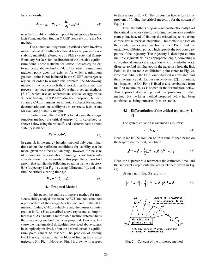
Figure 3 shows the Jacobian for G(x) in Eq. (15). Thenon-grayed-out blocks represent sparse matrices that are all

(10)

(11)

(12)

(13)

(14)

(15)

(16)

Fig. 3. Configuration of Jacobian.

29

zero. Below, the equations for blocks (1) through (4) in Fig.3 are given. Note that the preobtained Exit Point are usedin initial estimates for Eq. (16) with respect to all δ.

Block 1

Note that I is an n × n unit matrix.Block 2

ε is a scalar variable, and so block 2 represents an (m + 1)× n vertical vector.

Block 3

This is the flow Jacobian based on Eq. (13).Block 4

Note that M = [M1 M2 ⋅ ⋅ ⋅ Mn].

5. Simulations

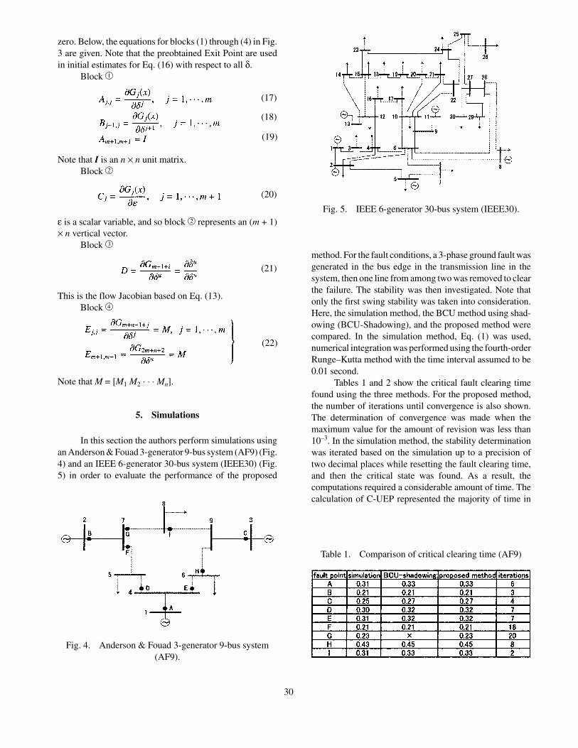
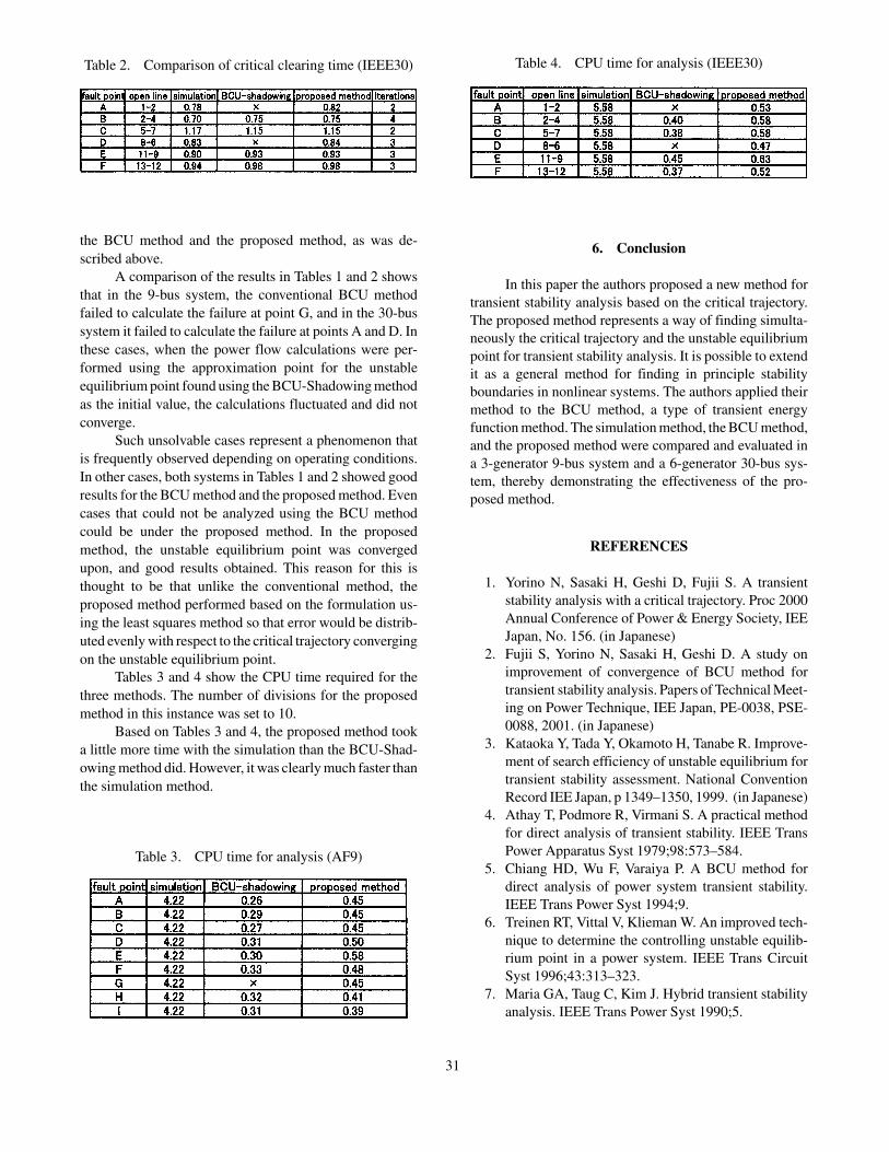
In this section the authors perform simulations usingan Anderson & Fouad 3-generator 9-bus system (AF9) (Fig.4) and an IEEE 6-generator 30-bus system (IEEE30) (Fig.5) in order to evaluate the performance of the proposed

method. For the fault conditions, a 3-phase ground fault wasgenerated in the bus edge in the transmission line in thesystem, then one line from among two was removed to clearthe failure. The stability was then investigated. Note thatonly the first swing stability was taken into consideration.Here, the simulation method, the BCU method using shad-owing (BCU-Shadowing), and the proposed method werecompared. In the simulation method, Eq. (1) was used,numerical integration was performed using the fourth-orderRunge–Kutta method with the time interval assumed to be0.01 second.

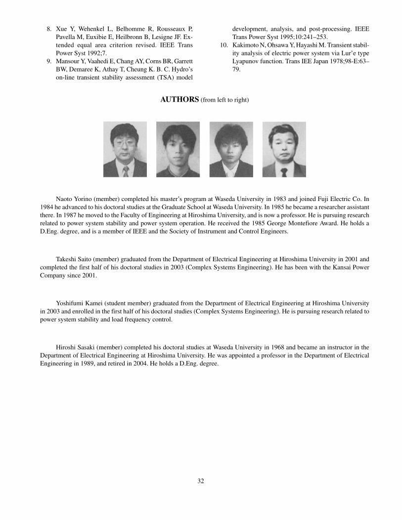
Tables 1 and 2 show the critical fault clearing timefound using the three methods. For the proposed method,the number of iterations until convergence is also shown.The determination of convergence was made when themaximum value for the amount of revision was less than10–3. In the simulation method, the stability determinationwas iterated based on the simulation up to a precision oftwo decimal places while resetting the fault clearing time,and then the critical state was found. As a result, thecomputations required a considerable amount of time. Thecalculation of C-UEP represented the majority of time in

(19)

(17)

(18)

(20)

(21)

(22)

Fig. 4. Anderson & Fouad 3-generator 9-bus system(AF9).

Fig. 5. IEEE 6-generator 30-bus system (IEEE30).

Table 1. Comparison of critical clearing time (AF9)

30

the BCU method and the proposed method, as was de-scribed above.

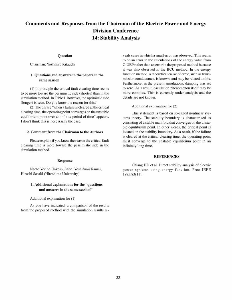
A comparison of the results in Tables 1 and 2 showsthat in the 9-bus system, the conventional BCU methodfailed to calculate the failure at point G, and in the 30-bussystem it failed to calculate the failure at points A and D. Inthese cases, when the power flow calculations were per-formed using the approximation point for the unstableequilibrium point found using the BCU-Shadowing methodas the initial value, the calculations fluctuated and did notconverge.

Such unsolvable cases represent a phenomenon thatis frequently observed depending on operating conditions.In other cases, both systems in Tables 1 and 2 showed goodresults for the BCU method and the proposed method. Evencases that could not be analyzed using the BCU methodcould be under the proposed method. In the proposedmethod, the unstable equilibrium point was convergedupon, and good results obtained. This reason for this isthought to be that unlike the conventional method, theproposed method performed based on the formulation us-ing the least squares method so that error would be distrib-uted evenly with respect to the critical trajectory convergingon the unstable equilibrium point.

Tables 3 and 4 show the CPU time required for thethree methods. The number of divisions for the proposedmethod in this instance was set to 10.

Based on Tables 3 and 4, the proposed method tooka little more time with the simulation than the BCU-Shad-owing method did. However, it was clearly much faster thanthe simulation method.

6. Conclusion

In this paper the authors proposed a new method fortransient stability analysis based on the critical trajectory.The proposed method represents a way of finding simulta-neously the critical trajectory and the unstable equilibriumpoint for transient stability analysis. It is possible to extendit as a general method for finding in principle stabilityboundaries in nonlinear systems. The authors applied theirmethod to the BCU method, a type of transient energyfunction method. The simulation method, the BCU method,and the proposed method were compared and evaluated ina 3-generator 9-bus system and a 6-generator 30-bus sys-tem, thereby demonstrating the effectiveness of the pro-posed method.

REFERENCES

1. Yorino N, Sasaki H, Geshi D, Fujii S. A transientstability analysis with a critical trajectory. Proc 2000Annual Conference of Power & Energy Society, IEEJapan, No. 156. (in Japanese)

2. Fujii S, Yorino N, Sasaki H, Geshi D. A study onimprovement of convergence of BCU method fortransient stability analysis. Papers of Technical Meet-ing on Power Technique, IEE Japan, PE-0038, PSE-0088, 2001. (in Japanese)

3. Kataoka Y, Tada Y, Okamoto H, Tanabe R. Improve-ment of search efficiency of unstable equilibrium fortransient stability assessment. National ConventionRecord IEE Japan, p 1349–1350, 1999. (in Japanese)

4. Athay T, Podmore R, Virmani S. A practical methodfor direct analysis of transient stability. IEEE TransPower Apparatus Syst 1979;98:573–584.

5. Chiang HD, Wu F, Varaiya P. A BCU method fordirect analysis of power system transient stability.IEEE Trans Power Syst 1994;9.

6. Treinen RT, Vittal V, Klieman W. An improved tech-nique to determine the controlling unstable equilib-rium point in a power system. IEEE Trans CircuitSyst 1996;43:313–323.

7. Maria GA, Taug C, Kim J. Hybrid transient stabilityanalysis. IEEE Trans Power Syst 1990;5.

Table 3. CPU time for analysis (AF9)

Table 2. Comparison of critical clearing time (IEEE30) Table 4. CPU time for analysis (IEEE30)

31

8. Xue Y, Wehenkel L, Belhomme R, Rousseaux P,Pavella M, Euxibie E, Heilbronn B, Lesigne JF. Ex-tended equal area criterion revised. IEEE TransPower Syst 1992;7.

9. Mansour Y, Vaahedi E, Chang AY, Corns BR, GarrettBW, Demaree K, Athay T, Cheung K. B. C. Hydro’son-line transient stability assessment (TSA) model

development, analysis, and post-processing. IEEETrans Power Syst 1995;10:241–253.

10. Kakimoto N, Ohsawa Y, Hayashi M. Transient stabil-ity analysis of electric power system via Lur’e typeLyapunov function. Trans IEE Japan 1978;98-E:63–79.

AUTHORS (from left to right)

Naoto Yorino (member) completed his master’s program at Waseda University in 1983 and joined Fuji Electric Co. In1984 he advanced to his doctoral studies at the Graduate School at Waseda University. In 1985 he became a researcher assistantthere. In 1987 he moved to the Faculty of Engineering at Hiroshima University, and is now a professor. He is pursuing researchrelated to power system stability and power system operation. He received the 1985 George Montefiore Award. He holds aD.Eng. degree, and is a member of IEEE and the Society of Instrument and Control Engineers.

Takeshi Saito (member) graduated from the Department of Electrical Engineering at Hiroshima University in 2001 andcompleted the first half of his doctoral studies in 2003 (Complex Systems Engineering). He has been with the Kansai PowerCompany since 2001.

Yoshifumi Kamei (student member) graduated from the Department of Electrical Engineering at Hiroshima Universityin 2003 and enrolled in the first half of his doctoral studies (Complex Systems Engineering). He is pursuing research related topower system stability and load frequency control.

Hiroshi Sasaki (member) completed his doctoral studies at Waseda University in 1968 and became an instructor in theDepartment of Electrical Engineering at Hiroshima University. He was appointed a professor in the Department of ElectricalEngineering in 1989, and retired in 2004. He holds a D.Eng. degree.

32

Comments and Responses from the Chairman of the Electric Power and EnergyDivision Conference14: Stability Analysis

Question

Chairman: Yoshihiro Kitauchi

1. Questions and answers in the papers in thesame session

(1) In principle the critical fault clearing time seemsto be more toward the pessimistic side (shorter) than in thesimulation method. In Table 1, however, the optimistic side(longer) is seen. Do you know the reason for this?

(2) The phrase “when a failure is cleared at the criticalclearing time, the operating point converges on the unstableequilibrium point over an infinite period of time” appears.I don’t think this is necessarily the case.

2. Comment from the Chairman to the Authors

Please explain if you know the reason the critical faultclearing time is more toward the pessimistic side in thesimulation method.

Response

Naoto Yorino, Takeshi Saito, Yoshifumi Kamei, Hiroshi Sasaki (Hiroshima University)

1. Additional explanations for the “questionsand answers in the same session”

Additional explanation for (1)

As you have indicated, a comparison of the resultsfrom the proposed method with the simulation results re-

veals cases in which a small error was observed. This seemsto be an error in the calculations of the energy value fromC-UEP rather than an error in the proposed method becauseit was also observed in the BCU method. In the energyfunction method, a theoretical cause of error, such as trans-mission conductance, is known, and may be related to this.Furthermore, in the present simulations, damping was setto zero. As a result, oscillation phenomenon itself may bemore complex. This is currently under analysis and thedetails are not known.

Additional explanation for (2)

This statement is based on so-called nonlinear sys-tems theory. The stability boundary is characterized asconsisting of a stable manifold that converges on the unsta-ble equilibrium point. In other words, the critical point islocated on the stability boundary. As a result, if the failureis cleared at the critical clearing time, the operating pointmust converge to the unstable equilibrium point in aninfinitely long time.

REFERENCES

Chiang HD et al. Direct stability analysis of electricpower systems using energy function. Proc IEEE1995;83(11).

33