A new method of image denoising based on cellular neural

*Corresponding author Email address: [email protected]

Songklanakarin J. Sci. Technol. 40 (3), 522-533, May - Jun. 2018

Original Article

A new method of image denoising based on cellular neural networks

Gangyi Hu1, 2* and Sumeth Yuenyong3

1 School of Science and Technology, Shinawatra University, Phaya Thai, Bangkok, 10400 Thailand

2 College of Big Data and Intelligence Engineering,

Southwest Forestry, Kunming, Yunnan, 650224 China

3 Department of Computer Engineering, Faculty of Engineering, Mahidol University, Salaya Campus, Phutthamonthon, Nakhon Pathom, 73170 Thailand

Received: 17 February 2016; Revised: 27 October 2016; Accepted: 7 February 2017

Abstract This paper presents an edge constraint adaptive filtering algorithm based on cellular neural networks for image

denoising. In the process of designing the three templates separately in cellular neural networks, the control template references the advantage of spatial filtering denoising. It resembles a spatial domain denoising filter. The feedback template sets as a matrix which generated by a high pass filter to achieve edge preservation. The proposed method can not only achieve denoising, but also protect edges in an image. In the process of designing the threshold template, we use the different gray levels in an image to achieve the threshold adjustment adaptively. The experiment simulation results show that this algorithm is effective. Its denoising effect is much better than the mean filtering, median filtering, Gaussian filtering and the non local means method. And compared with the anisotropic diffusion algorithm, this algorithm is also better for the impulsive noise (salt & pepper noise), the Poisson noise and the comprehensive noise denoising. Due to the parallelism and possible hardware implementation of cellular neural network, it can achieve real time image denoising, which has a good application prospect.

Keywords: cellular neural networks, image denoising, spatial filtering, adaptive edge constraint

1. Introduction The process of image acquisition, conversion and

transmission is often influenced by external factors leading in the appearance of some random, discrete or isolated points on the original image, these points are not predictable and can be represented by stochastic process, these are noise. In image processing, denoising is a research hotspot, the main goal for denoising is to separate the useful signal and noise, and to restore the true image.

The traditional image denoising method is mainly concentrated on local analysis in spatial or frequency domain,

such as the mean filtering, gray-scale transformation, histo-gram equalization and median filtering. Their basic idea is to use the neighborhood of a pixel as mean or median instead of noise, while suppressing the noise, these methods will destroy image edge and other important information, they also declined the quality of the image. In 2006, Buades proposed a non local means denoising method. The basic idea is to measure the similarity of image through the block to construct an average weight. This method only has good denoising effect in the relatively flat areas, but in the edge region which has rich detail information, the denoising effect is very weak (Buades, 2006; Koeppl & Chua, 2007).

In recent years, due to the parallel and hardware implementation of cellular neural networks (CNN), its application in image processing has become a hot topic of research. In the aspect of using CNN for image denoising, the

G. Hu & S. Yuenyong / Songklanakarin J. Sci. Technol. 40 (3), 522-533, 2018 523

previous researches were mainly used other image denoising algorithms (such as Partial Differential Equations algorithm), and then transplanted them with CNN for implementation. But few reports directly use the CNN template parameters design as a spatial filter for image denoising (Slavova, 2011).

This paper starts from the characteristics of CNN, and explores the image denoising templates which are an adaptation of cellular neural networks. The process of designing the template, references the spatial filtering denoising method, and also considers the requirement of preserving image details. The difference of edge direction of each pixel accessed for judging whether it has useful edge information, and then protects it. At the same time, in the process of threshold template design, its value is adjusted through the gray image pixel values, which are adaptive. This method for image denoising is simple and can be easily implemented by hardware.

The noise type of pollution image can be divided into additive noise and multiplicative noise according to the relationship of noise and the original image. Assume that the original image is ( )X i , the noise is ( )N i , if the mixed signal superposition meets the form is ( ) ( ) ( )V i X i N i , then it is called additive noise; if the mixed signal superposition meets the form ( ) ( ) ( )* ( )V i X i N i X i , it is called multiplicative noise.

The pollution noises in an image usually involved Gaussian noise, impulsive noise (also known as the salt & pepper noise), speckle noise, Poisson noise and comprehen-sive noise. In this paper, we will mainly discuss the denoising of these five kinds of noise in the image

2. The Contribution of This Paper

(1) Applying the theory of cellular neural networks to image denoising directly uses the CNN template parameters design as a spatial filter for image denoising. This is different from the previous denoising algorithm such as Slavova’s method. That method first used the algorithm such as Partial Differential Equations for image denoising, and then trans-planted this algorithm with CNN for hardware realization. Our algorithm opened up a new method for image denoising.

(2) In the templates design process, we first con-sider the three templates designed separately, and propose the method as referenced to classical spatial filtering template, preserve the edge information of an image, and automatically adjust the threshold value according to the gray level.

(3) Through seven comparison experiments we show the use of cellular neural networks directly for image denoising with the templates designed separately to obtain their parameters, this can improve the image denoising quality for impulsive noise (salt& pepper noise), Poisson noise and comprehensive noise. However, for Gaussian noise and spec-kle noise, its effect is not as better than that of the anisotropic diffusion filter algorithm.

3. Research Background 3.1 The theory of spatial filter

The spatial filter theory involves moving a template

over each point in an image and replacing the pixel at the center of the neighborhood. It uses the value of the operation between the template and the pixels under the template. Different types of spatial filter just have different templates (Jyoti & Rupinder, 2014; Santhanam & Radhika, 2011).

3.1.1 Neighbor average filter

The neighbor average filter is a local spatial pro-cesssing method. Each of its pixel value is decided by the average of several pixels value in the neighborhood, the mathematical formula is , , , ,i i v i i vY Mean f f f .

3.1.2 Median filter

Median filter is a nonlinear filter, the basic principle is using the median value of the pixel in a neighborhood to replace the pixel in the center of the template, the mathe-matical formula is , , , ,i i v i i vY Med f f f .

3.1.3 Gaussian filter

Gaussian filter is a smoothing filter which selects

the template value according to the shape of the Gaussian distribution. The variance parameter determines the effective width of the Gaussian filter. The Gaussian filter can remove the noise, but also blur the image, the Gaussian distribution mathematical formula is

2

2212

i

iY e

.

3.1.4 Edge preserving filter

Edge preserving filter mainly refers the anisotropic diffusion partial differential equation. The limit of the linear filter operator is a differential operator and it is a heat con-duction equation. It can be regarded as a homogeneous iso-tropic heat diffusion process. When considered using the prior information of the image, it reduces the diffusion of the edges and preserves the edges better. The gradient operator is used as an edge detector to control the speed of diffusion. Perona and Malik have proposed the anisotropic diffusion method, and this method has received wide attention. It uses the mathematical formula is ( ( , , ) ) ( , , ) .Y div c x y t Y c x y t Y c yi . The diffusion model and its numerical solution have been greatly developed. The biggest advantage of the anisotropic diffusion filtering method is realizing the nonlinear filtering operation of the image, wherever the noise can be eliminated and edge can be better preserved (Perona & Malik, 1990).

524 G. Hu & S. Yuenyong / Songklanakarin J. Sci. Technol. 40 (3), 522-533, 2018

3.2 Cellular neural networks Cellular neural networks (CNN) was proposed by

Chua L.O. and Yang L. in 1988 in which it was used in image, video signal processing, robotic, biological visions and high brain function (Chua & Yang, 1988 ).

It consists of a large number of cellular com-ponents, and only adjacent cells can communicate directly. Each cell comprises only a linear capacitor, a nonlinear vol-tage controlled current source and a small amount of linear circuit resistances. A group of cells are interconnected within a limited region. All state variables have continuous value, but the time value does not need to be continuous. This allows for the realization of real-time signal processing in the digital domain (Wang, 2009).

3.3 The cellular neural networks model

Figure 1 shows cellular neural networks with 3*3

local interconnection model structure. In fact, the whole structure of CNN is composed of M*N cell components, and the cell in the missing line and the missing column will only be connected by the neighboring cell. The cell which is not directly connected communicates by acting through dynamic propagation (Wei et al., 2014).

Figure 1. The model structure chart of cells in Cellular Neural

Network

The neighborhood of Nij(r) is defined in Equation 1:

(1) where 1 i M , 1 i N , r is the radius of the neigh-borhood of cellular Cij , and Cab is the neighbor cell of cellu-lar Cij .

In the M*N local interconnect model structure, any cell Cij , whose circuit model is composed by linear circuit and non-linear circuit. Each cell of Cij contains the input varia-bles, output variables, state variables and threshold. The dyna-mic first-order nonlinear differential equation for cellular Cij can be represented in Equation 2 (Tukel & Yalcin, 2010).

, ( )

, ( )

( ) ( )( )ij ij

kl klk l N rx ij

kl kl ijk l N rij

dx t x tC A y t

dt R

B u I

(2)

where xij is a state variable, ykl is an output variable, ukl is an input variable, Iij is the threshold, A is the feedback coefficient matrix and B is the control coefficient matrix.

The standard output equation of CNN is shown in Equation 3.

(3)

The input equation is shown in Equation 4.

NjMiEu ijij 1,1 (4)

The constraint equation is shown in Equation 5.

(5)

The output function of f(x) is a piecewise linear

function whose value is between [-1,1]. The adjustable parameters in CNN are A,B,I of cells which are called the neural network templates, they decide the direction and the function of the dynamic changes of the CNN. We will design the value of A,B,I to achieve the purpose of image denoising.

CNN is a nonlinear circuit, and the most effective method to analyze the convergence of linear circuit is the Lyapunov method, The Lyapunov function of CNN is shown in Equation 6 (Huaqing et al., 2011; Yoshihiro et al.,2012).

1( ) ( ) ( )2 ( , ) ( , )

1 2 ( ) ( )2 ( , ) ( , ) ( , )

( )( , )

E t A y t y tk l kl iji j k l

y t B u y tk l kl iji jR x i j i j k l

I y ti j iji j

(6)

According to the definition of Equation 6, as long as )(tE is bounded, and with the increasing time of t , )(tE

decreases monotonically, CNN is stable. On this basis and from the previous equation, we get the Equation 7.

( , ) ( , ) ( , ) ( , ) ( , ) ( , )

1 1( ) ( ) ( ) ( ) ( ) ( )2 2kl k l ij ij k l k l ij ij ij

i j k l i j i j k l i jE t A y t y t y t B u y t I y t

2

( , ) ( , ) ( , ) ( , ) ( , ) ( , )

1 1( ) ( ) ( ) ( ) ( ) ( )2 2kl kl ij ij kl kl ij ij ij

i j k l i j i j k l i jx

E t A y t y t y t B u y t I y tR

1( ) (| ( ) 1 | | ( ) 1 |) ( )2

y t x t x t f xij ij ij

( ) | max(| |,| |) ,1 ,1N r C a i b j r a M b Nij ab

| (0) | 1 1 ,1| | 1 1 ,1x i M j Niju i M j Nij


)(2

1|)(|.|)(|.||21

),(

2

, ),(

jiij

xijkl

ji lkkl ty

RtytyA

）（

|)(|.|||)(|.||.||),(),( ),(

ji

ijijijklji lk

kl tyItyuB (7)

Because of the state definition of CNN, we already

have the | | 1uij | | 1yij we can get the Equation 8.

2.||

21)(

),( ),(

xkl

ji lk RNMAtE ||||

),(),( ),(

jiij

ji lkkl IB

(8)

So )(tE is bounded. On the other hand, we compute

the time derivative of )(tE

),(),( ),(

)()()(1)(

)()()(ji

ijij

ij

ij

xkl

ij

ij

ij

ji lkkl ty

dttdx

dxtdy

Rty

dttdx

dxtdy

Adt

tdE

),(),( ),(

)()()()(

ji

ij

ij

ijij

ij

ij

ij

ji lkklkl dt

tdxdx

tdyI

dttdx

dxtdy

uB

(9)

By the output equation of the standard CNN which

is )(|)1)(||1)((|21)( xftxtxty ijijij , it can get

the Equation 10

1||,01||,1

)()(

ij

ij

ij

ij

xx

tdxtdy

(10)

Because Cij can only be connected with the adjacent

cell element, it can get the Equation 11. When ( )C N rij ij , it can get 0, 0A Bkl kl .

(11) We can get the Equation 12 according from the

Equation 9 to Equation 11.

,

( , ) ( , )

| | 1

( , ) ( , )

( ) ( )( ) -( )

1( )- ( )

( )

1( ) ( )

ij ij

i j ij

kl kl ij kl kl ijk j k jx

ij

xij

kl kl ij kl kl ijk j k jx

dx t dy tdE tdt dt dx t

A y t y t B u IR

dx tdt

A y t x t B u IR

(12)

Because the dynamic equation of cellular is shown in Equation 2, and we calculate it with the Equation 12, the

other is because C is the capacitance parameter with 0C , the Equation 12 can be changed as Equation 13.

( )( ) 02

| | 1

d x td E t Cd t d t

i j

x ij

(13)

We can be sure that )(tE is monotonically de-

creasing. That is to say that CNN always reduces the energy in the direction of movement, and eventually achieves a stable state, and the networks will finally reach a stable equilibrium point. 3.4 Image preprocessing

When we use the CNN for imagine processing, in

order to meet the CNN constraints, we must adjust the range of input values as the following (Huaiyin, 2007).:

(1) For the eight bit gray image, because of original pixel value of it is 0,1,..., 255 ,gij the uij , which is the

external input of the CNN, must satisfy | | 1uij ,so we must

take the range of gij to be -1 .0 , 1 .0 in a linear mapping as

shown in Equation 14 (Wei et al.,2014). (14)

The original image gray level of the 0 (black) is

mapped to the CNN 1.0 (black), and the original gray level of the 255 (white) is mapped to the CNN -1.0 (white), the rest of the gray values from small to large are mapped linearly to 1.0 until -1.0.

(2) For binary images, because of original pixel value is 0,1g ij , the value 0 (black) is mapped to the

CNN 1.0 (black), and the value 1 (white) is mapped to the CNN -1.0 (white). 4. The Edge Constraint Adaptive Filtering Algorithm Based on CNN

Aiming at the smooth edge limitation of spatial fil-

tering in image denoising, combined with the advantages of parallel and hardware implementation of CNN, this paper propose the edge constraint adaptive filtering algorithm based on CNN. We will focus on the following three questions.

(1) Due to the different sources of noise pollution and different environments for the image acquisition, there are great differences in the types of pollution. If we still use a single filtering algorithm it may not be able to obtain satis-factory denoising effect. This algorithm uses different filters which have best denoising effect for different types of noise, such as the Mean filter for Gaussian noise and speckle noise, the Median filter for salt & pepper noise and Poisson noise, and the Gaussian filter for comprehensive noise. The CNN control template parameter B setting, references the different spatial filters which can get the effect of filtering.

(1 2 / 255) 1.0, 1.0u gij ij


(2) Due to the spatial filtering in image denoising, some edge information will be lost. Therefore, in the processing of image pixels, because each pixel is gradually moved, so each pixel of edge gradient direction generally can be characterized by the four directions ( 0000 13590450 、、、 ). Through the direction, we can find the pixel which is adjacent to the pixel's gradient direction, and judge whether there is an edge in the four directions near the original pixel, The CNN feedback template parameter A setting uses the constraint high pass filter to protect the edge information (Feng et al., 2009).

(2) In the setting of threshold I, because the gray level of the pollution image is too concentrated or not even, if the whole image only uses one determined threshold, the noise signal cannot easily be separated. Through the gray value of the image to adjust the threshold parameter adaptively in order to solve the problem of uneven distribution of gray values which lose image’s characteristics after denoising.

In brief, the edge constraint adaptive filtering algorithm based on CNN has three functions: the control template B setting as spatial filter for filtering, the feedback template A setting as a constraint high pass filter for edge preserving, the threshold template I setting adaptively for clearly separating the signal and contrast effect.

4.1 How to design the control template B

In the dynamic equation of CNN, the time constant

R Cx reflects the speed of network dynamic change process. For simplification, assume that the parameter of the dynamic equation 1, 1C Rx . So the dynamic equation of CNN is shown in Equation 15.

( )( ) ( )

, ( ) , ( )

dx tijx t A y t B u Iij kl kl kl kl ijdt k l N r k l N rij ij

(15)

The Equation 15 can be simplified as Equation 16.

(16)

Where“*”is convolution. It means that the output ykl of every cell in the cell Cij neighborhood convolutes with the corresponding elements from the A template. The external input ukl convolutes with the corresponding elements from the B template, and then they are added.

If we do not consider the influence of the output feedback, and make the threshold I=0, the CNN state equation can be simplified again as Equation 17.

(17)

The Equation 17 means that, X is the image output

equal to the spatial filter B filter the input image U, the spatial filter’s principle is moving the template point by point in the image processing, and is comparing the relationship between the filter coefficient and the correspond pixel area value which is swept by the template. Thus, for the B template design, we can use a spatial filtering template, such as the Mean filter template for Gaussian noise and speckle noise, the Median

filter template for salt & pepper noise and Poisson noise, the Gaussian filter template for comprehensive noise. The CNN template parameters setting references the different spatial filters. This can achieve filtering function.

4.2 How to design the feedback template A

In the equation of the CNN state, the feedback

template A will directly affect the output ykl. In the design of the template A for image denoising, we set a matrix which is generated by a high filter to achieve edge constraint.

The high pass filter will enlarge the edge and noise at the same time, and on the other hand, when noise is reduced, the edge will also be smoothed. Therefore, in order to protect the edge information, firstly the directions ( 0000 13590450 、、、 ) of an edge going through a pixel are identi-fied, and then a high pass filter is used to protect the edge information.

If we define the edge direction discriminant called P1,P2,P3,P4 to determine whether there is edge of the four directions, the discriminant calculation formulas can be shown in Equation 18 (Feng et al., 2009).

|)1,()1,(|0|)1,()1,(|1

1 jifjifjifjif

P

|)1,1()1,1(|0

|)1,1()1,1-(|12 jifjif

jifjifP

|),1(),1(|0

|),1(),1-(|13 jifjif

jifjifP

|)1,1()1-,1(|0

|)1,1()1-,1-(|14 jifjif

jifjifP

(18) where, is a constant, the high pass filter which corresponds to the edge direction discriminant called C1,C2,C3,C4 the calculation formula are shown in Equation 19.

0001-21-000

41

1C

,

01-002001-0

41

2C

,

1-00020001-

41

3C

,

001-0201-00

41

4C

(19)

If we use the isotropic high pass filter called 0C as a reference, and the direction operator of every edge direction added, we can get the compound formula as shown in Equation 20.

)(1

1 4

104

1

i

ii

ii

CPCP

C

(20)

* *X A Y B U I

*X B U


1-1-1-1-81-1-1-1-

161

0C

In the setting of designing the template A, we just set it as the equation 20 equal to C. Because each pixel is gradually moving to determine whether there is edge infor-mation, the discriminant of each pixel called P1,P2,P3,P4 is different (the value of P1,P2,P3,P4 is one of the sixteen combinations from 0000 to 1111), The difference value of P1,P2,P3,P4 leads to the difference of C in equation 20, thus the feedback template A has different value of each pixel. That is to say, the feedback template A is dynamically changed in the range of sixteen kinds according to the Equation 20. 4.3 How to design the threshold template I

Because the noisy image background is not even,

the fixed threshold I is unable to achieve the ideal effect. We assume that the original image gray value is

)2550( ijij gg , then in the process of using CNN for

image denoising, we consider the threshold of I will change with ijg .

Suppose ijij I , and without considering the

influence of the output feedback, the state Equation 16 of CNN can be simplified as equation 21.

ijrNlk

klklijij

uBx -)(,

(21)

According to the CNN input range, the external

input iju of CNN is in Equation 22.

0.1,0.1)255/21( ijij gu (22)

We change the Equation 21 according to the Equa-

tion 22 and can obtain the Equation

ijrNlk

ijklijij

gBx -)255/21.()(,

(23)

where we can make the value of the

ij increasing as the

original image gray value ijg increases becauseijijI ,

and the output function of the CNN, which is

|)1)(||1)((|21)( txtxty ijijij

. Another reason is that

only the neighboring cells that are connected interact with each other. So the threshold template ijI of CNN is set as

Equation 24.

255/).(1)(,

rNlk

klijijij

BgI (24)

Each cell has a corresponding threshold Iij, the value

of the threshold Iij is adjusted like the equation 24 according to the image gray value adaptive.

When we set the template A, B, I according to the above method, the cells will gradually update to the direction of decreased power based on the dynamic equation of CNN and ultimately achieve stability. It should be used for different image denoising. 5. The Simulation and Experimental Analysis

In order to verify the effectiveness of this algorithm,

we set up the experiment as follows. They use CNN for different image denoising, compare it with the image denoising methods like mean filtering, median filtering, the Gaussian filtering, non- local means and anisotropic diffusion filtering. The experimental environment is type of CPU AMD2.50G, 4.00G memory, Matlab7.0.The test image is the size of 256*256 standard test image which is “Cameraman”, “Lena”, ” Baboon” “Sculpture”, “House”, “Chili” and “Lady”, The Cameraman image is injected with Gaussian noise with mean 0, and variance is 0.01. The Lena image is injected with salt & pepper noise with density is 0.2. The Baboon image is injected with speckle noise with variance is 0.04. The Sculpture image is injected with Poisson noise, The House image is injected with Gaussian noise and salt & pepper noise mixed together, The Chili image is injected with the speckle noise and the salt & pepper noise mixed together, The Lady image is injected with Gaussian noise and Poisson noise mixed together.

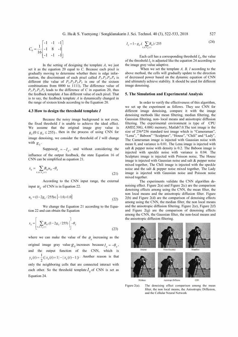
The experiments validate the CNN algorithm de-noising effect. Figure 2(a) and Figure 2(c) are the comparison denoising effects among using the CNN, the mean filter, the non local means and the anisotropic diffusion filter. Figure 2(b) and Figure 2(d) are the comparison of denoising effects among using the CNN, the median filter, the non local means and the anisotropic diffusion filtering. Figure 2(e), Figure 2(f) and Figure 2(g) are the comparison of denoising effects among the CNN, the Gaussian filter, the non-local means and the anisotropic diffusion filtering.

Figure 2(a). The denoising effect comparison among the mean

filter, the non local means, the Anisotropic Diffusion, and the Cellular Neural Network


Figure2 (b). The denoising effect comparison among the median


Figure2 (c). The denoising effect comparison among the mean


Figure2 (d). The denoising effect comparison among the median


Figure 2 (e). The denoising effect comparison among the Gaussian


Figure2 (f). The denoising effect comparison among the Gaussian filter, the non local means, the Anisotropic Diffusion, and the Cellular Neural Network

Figure2 (g). The denoising effect comparison among the Gaussian



In order to detect the image denoising effect quanti-tatively, in this paper, the peak signal to noise ratio (PSNR) is used to evaluate the image denoising effect. The formula is shown in Equation 25.

225510log

1 2( ),,( )

PSNR

x xi ji jMN ij

(25)

In the Equation 25, x is the original image without noise, is the image after denoising, M and N are the number of rows and columns of the image. Every algorithm denoising effect as indicated by the PSNR value in Table 1. Table1. The PSNR value of using different denoising methods (dB)

The Table 1 shows the PSNR value compared

between the denoising effect using the CNN and other algorithms. It can be seen that the effecting the denoising algorithm based on CNN is obviously better than the other traditional denoising algorithms. When comparing the CNN algorithm with the anisotropic diffusion filtering, this algorithm for impulsive noise (salt & pepper noise), the Poisson noise and the comprehensive noise denoising are better than the anisotropic diffusion filtering. Figure 3(a) to Figure 3(g) are the comparison of using image edge detection algorithms to protect the edge during denoising. From the figures, we can see our algorithm for the Gaussian noise and speckle noise denoising, the edge protective effect is not as good as the anisotropic diffusion filtering, but with the impulsive noise (salt & pepper noise), the Poisson noise and the comprehensive noise, the edge protection effect is better than with the anisotropic diffusion filtering. At the same time, in the denoising and edge pro-

tection, our algorithm is much better than the NLMeans algorithm and other traditional denoising algorithm.

Figure 3(a). The denoising edge protect comparison among the Cellular Neural Network, the Anisotropic Diffusion, the non local means, and the mean filter (noise type, Gaussian)

Figure 3(b). The denoising edge protect comparison among the Cellular Neural Network, the Anisotropic Diffusion, the non local means, and the mean filter (noise type, Salt & Pepper)

Figure 3(c). The denoising edge protect comparison among the Cellular Neural Network, the Anisotropic Diffusion, the non local means, and the mean filter (noise type, Speckle

Test image (256* 256)

Noise type

Using different spatial

filter for image

denoising

Using Non Local

Mean for image

denoising

Using Anisotropic Diffusion for image denoising

Using CNN for

image denoising

Camera- man

Gaussian 24.54 (mean filter)

25.71 27.39 25.92

Lena Salt & Pepper

24.95 (median filter)

26.31 24.53 26.87

Baboon Speckle 23.99 (mean filter)

26.04 27.72 27.08

Sculpture Poisson 24.17 (median filter)

25.84 25.65 26.23

House Gaussian and Salt & Pepper

23.42 (Gaussian

filter)

24.63 24.73 24.93

Chili Speckle and Salt & Pepper

25.52 (Gaussian

filter)

26.29 25.85 26.75

Lady Gaussian and Poisson

24.66 (Gaussian

filter)

23.93 24.95 25.08

x


Figure 3(d). The denoising edge protect comparison among the

Cellular Neural Network, the Anisotropic Diffusion, the non local means, and the mean filter (noise type, Poisson)

Figure 3(e). The denoising edge protect comparison among the

Cellular Neural Network, the Anisotropic Diffusion, the non local means, and the mean filter (noise type, Gaussian and Salt & Pepper)

Figure 3(f). The denoising edge protect comparison among the

Cellular Neural Network, the Anisotropic Diffusion, the non local means, and the mean filter (noise type, Speckle and Salt & Pepper)

Figure 3(g). The denoising edge protect comparison among the

Cellular Neural Network, the Anisotropic Diffusion, the non local means, and the mean filter (noise type, Gaussian and Poisson)

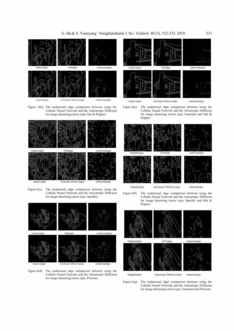
Figure 4(a) to Figure 4(g) are the comparison of the

undetected edge information, using the original image edge subtracting the denoising image edge, and the denoising algorithm using the CNN and the Anisotropic Diffusion methods. Table 2 show the comparison of undetected edge rate between using the CNN and the Anisotropic Diffusion for image denoising. Figure 4(a) to Figure 4(g) and Table 2 show that in the noise such as impulsive noise (salt & pepper noise), Poisson noise and comprehensive noise, if it uses the CNN for image denoising the rate of the undetected edge is low, and the protection effect of the image is better.

Figure 4(a). The undetected edge comparison between using the

Cellular Neural Network and the Anisotropic Diffusion for image denoising (noise type, Gaussian)


Figure 4(b). The undetected edge comparison between using the

Cellular Neural Network and the Anisotropic Diffusion for image denoising (noise type, Salt & Pepper)

Figure 4(c). The undetected edge comparison between using the

Cellular Neural Network and the Anisotropic Diffusion for image denoising (noise type, Speckle)

Figure 4(d). The undetected edge comparison between using the

Cellular Neural Network and the Anisotropic Diffusion for image denoising (noise type, Poisson)

Figure 4(e). The undetected edge comparison between using the

Cellular Neural Network and the Anisotropic Diffusion for image denoising (noise type, Gaussian and Salt & Pepper)

Figure 4(f). The undetected edge comparison between using the

Cellular Neural Network and the Anisotropic Diffusion for image denoising (noise type, Speckle and Salt & Pepper)

Figure 4(g). The undetected edge comparison between using the

Cellular Neural Network and the Anisotropic Diffusion for image denoising (noise type, Gaussian and Poisson)


Table 2. The undetected edge rate comparison between using the cellular neural network and the Anisotropic Diffusion for image denoising

The experiments show that, if the template of CNN

is properly set in above method, it can realize the image denoising and edge protection. The implementation for this is shown in appendix A. 6. Conclusions

This paper proposes the edge constraint adaptive

filtering algorithm based on CNN. It is a kind of filtering algorithm that can achieve a variety of functions. For different types of noise, it uses different spatial template to set the different CNN template parameters, which can achieve different forms of filtering, and it has good flexibility. In addition, it can protect the edge information. The adaptive threshold can also obtain contrast effect obviously. The three module parameters are designed separately and directly in the CNN for denoising; this is different from the previous CNN denoising algorithms, which first uses the Partial Differential Equations denoising, and then transplant it with CNN for implementation.

From the simulation results we can see that, compared with the state-of-the-art method such as anisotropic diffusion filter algorithm, the algorithm in this paper is better for impulsive noise (salt & pepper noise), Poisson noise and comprehensive noise denoising. But for Gaussian noise and speckle noise, even though it's worse than anisotropic diffusion, it's still better than non-local means and other traditional denoising methods. This algorithm which directly sets the CNN parameter as filter, is simple and can be easily implemented by hardware due to its parallel structure.

However, this proposed method also has some limitations. The first limitation is the selection of spatial filter (control template B) for different noise cannot realize automatically. The second limitation is in the process of setting the feedback template A; the discrimination cannot be perfect because there are trade-offs between the image denoising and the edge details protection; if the constant value of in equation 18 is set large, it will lose some edge detail information, if the constant value of is set low, it may judge

the noise as edge information, which cannot achieved the purpose of denoising.

In our research, the selection of these spatial filter (control template B) and the discriminant constant value of in equation 18 are mainly based on the result of some experiments to achieve the function, there may be a way to automatically choose the control template B and the constant value of optimally, which could be selection in functionally. References Ahmed, S., Dey, S., & Sarma. (2011). Image texture classi-

fication using artificial neural network. Proceeding of the 2nd National Conference on Emerging Trends and Applications in Computer Science, Shilong, India 2011, 1–4.

Buades. (2006). A review of image denoising algorithms with a new one. Multiscale Modeling and Simulation, 4, 490–530.

Chua, L. O., & Yang, L. (1988). Cellular neural networks: Theory, IEEE Transactions on Circuits and Sys-tems, 10, 1257–1272.

Chua, L. O., & Yang, L. (1988).Cellular neural networks: Application, IEEE Transactions on Circuits and Systems, 10, 1273–1290.

Feng, Q., Shenglin, Y. U., & Wei, Z. (2009). A novel image restoration algorithm using cellular neural networks. Journal of Image and Graphics, 3, 430–434.

Huai ,Y. W. (2007). Research on Application of cellular neural network in image processing (Doctoral thesis, Nanjing University of Aeronautics and As-tronautics, Jiangsu, China)

Huaqing, L., Xiaofeng, L., Chuandong, L, Hongyu, H., & Chaojie, L. (2011). Edge detection of noisy images based on cellular neural networks. Communications in Nonlinear Science and Number Simulation, 16, 3746–3759.

Jyoti, S., & Rupinder, K. (2014). An efficient technique of image noising and denoising using neuro- fuzzy and SVM (Support vector machine)-A Survey. Inter-national Journal of Computer Science and Informa-tion Technologies, 2, 2038–2041.

Koeppl, H., & Chua, L. O., (2007). An adaptive cellular non-linear network and its application. Proceeding of 2007 International Symposium on Nonlinear Theory and its Applications NOLTA'07, 15-18. Retrieved from http://www.ieice.org/proceedings/NOLTA200 7/articles/17PM1-B-1-Koeppl.pdf

Perona, P., & Malik, J. (1990). Scale-space and edge detection using anisotropic diffusion. IEEE Transactions on Pattern Analysis and Machine Intelligence, 12, 629-639.

Santhanam,T., & Radhika, S. (2011). Applications of neural networks for noise and filter classification to enhance the image quality. International Journal of Computer Science, 8, 314–317.

Slavova, A. (2011). A novel cnn based image denoising model. Proceeding of the 20th European Conference on Circuit Theory and Design, Linkoping, Sweden 2011, 226–229. Retrieved from https://ieeexplore. ieee.org/ stamp/stamp.jsp?tp=&arnumber=6043323

Test image (256*256)

Noise type

undetected edge error

rate (using CNN

image denoising)

undetected edge error

rate (using

Anisotropic Diffusion for image denoising)

Cameraman Gaussian 10.32% 7.22% Lena Salt & Pepper 8.89% 13.6% Baboon Speckle 27.6% 19.8% Sculpture Poisson 13.76% 15.8% House Gaussian and

Salt & Pepper 5.79% 6.53%

Chili Speckle and Salt & Pepper

13.48% 14.39%

Lady Gaussian and Poisson

12.11% 13.64%


Tukel, M., & Yalcin, M. E. (2010). A new architecture for cellular neural network on reconfigurable hardware with an advance memory allocation method. Pro-ceeding of the 12th International Workshop on Cellular Nanoscale Networks and their Applica-tions, Berkeley, USA. 2010, 1–6.

Veerakumar, T., Esakkirajan, S., & Vennila, L. (2014). Edge preserving adaptive anisotropic diffusion filter approach for the suppression of impulse noise in images, International Journal of Electronic and Communications, 5, 442–452.

Wang, J. L.,Yang, C. L., & Sun, C. (2009). A novel algorithm for edge detection of remote sensing image based on CNN and PSO. Proceeding of the 2nd International Congress on Image and Signal Processing, Tianjin, China 2011, 1–5. Retrieved from https://ieeexplore. ieee. org/stamp/stamp.jsp?tp=&arnumber=5304415

Wei, W., Li, J. Y, Yuting, X., & Youwei, A. (2014). Edge detection of infrared image with CNN_DGA algo-rithm, Optik International Journal for Light and Electron Optics,1, 464–467.

Yoshihiro, K.,Yoko, U., & Yoshifumi, N. (2012). Investi-gation of image denoising by cellular neural networks with effect from friend of a friend. Pro-ceeding of IEEE Workshop on Nonlinear Circuit Networks, Tokushima, Japan 2012, 105–108.

Appendix A

1. Read image ; 2. Normalization the pixel value adjust according to equation (14); 3. B :set as a special spatial filter; 4. A: set as equation (20); 5. I: set as equation (24); 6. For row from 1 to N 7. For column from 1 to N 8. A: adjust according to equation (20); 9. I: adjust according to equation (24); 10. Image[row,column]=equation (15); 11. End 12. End

Documents

A new method of image denoising based on cellular neural